NBER WORKING PAPER SERIES

TAYLOR RULE EXCHANGE RATE FORECASTING DURING THE FINANCIALCRISIS

Tanya MolodtsovaDavid Papell

Working Paper 18330http://www.nber.org/papers/w18330

NATIONAL BUREAU OF ECONOMIC RESEARCH1050 Massachusetts Avenue

Cambridge, MA 02138August 2012

We are grateful to Charles Engel, Jan Groen, Michael McCracken, Barbara Rossi, Michael Rosenberg,Ken West, and participants in seminars at the Bank of France, Paris School of Economics, Universityof California at Davis, 2010 SEA meetings, 2011 AEA meetings, the Conference on Exchange Ratesat Duke University, the 22nd (EC)2 Conference on “Econometrics for Policy Analysis: After the Crisisand Beyond”, and the 2012 ISOM meetings for their comments. The views expressed herein are thoseof the authors and do not necessarily reflect the views of the National Bureau of Economic Research.¸˛¸˛

NBER working papers are circulated for discussion and comment purposes. They have not been peer-reviewed or been subject to the review by the NBER Board of Directors that accompanies officialNBER publications.

© 2012 by Tanya Molodtsova and David Papell. All rights reserved. Short sections of text, not to exceedtwo paragraphs, may be quoted without explicit permission provided that full credit, including © notice,is given to the source.

Taylor Rule Exchange Rate Forecasting During the Financial CrisisTanya Molodtsova and David PapellNBER Working Paper No. 18330August 2012JEL No. C22,F31

ABSTRACT

This paper evaluates out-of-sample exchange rate predictability of Taylor rule models, where the centralbank sets the interest rate in response to inflation and either the output or the unemployment gap, forthe euro/dollar exchange rate with real-time data before, during, and after the financial crisis of 2008-2009.While all Taylor rule specifications outperform the random walk with forecasts ending between 2007:Q1and 2008:Q2, only the specification with both estimated coefficients and the unemployment gap consistentlyoutperforms the random walk from 2007:Q1 through 2012:Q1. Several Taylor rule models that areaugmented with credit spreads or financial condition indexes outperform the original Taylor rule models.The performance of the Taylor rule models is superior to the interest rate differentials, monetary, andpurchasing power parity models.

Tanya Molodtsova1602 Fishburne DrDepartment of EconomicsEmory UniversityAtlanta, GA 30322tmolodt@emory.edu

David PapellDepartment of EconomicsUniversity of HoustonHouston, TX 77204dpapell@uh.edu

1

1. Introduction

The past few years have seen a resurgence of academic interest in out-of-sample exchange rate

predictability. Gourinchas and Rey (2007), using an external balance model, Engel, Mark, and West

(2008), using monetary, Purchasing Power Parity (PPP), and Taylor rule models, and Molodtsova and

Papell (2009), using a variety of Taylor rule models, all report successful results for their models vis-à-vis

the random walk null. There has even been the first revisionist response. Rogoff and Stavrakeva (2008)

criticize the three above-mentioned papers for their reliance on the Clark and West (2006) statistic,

arguing that it is not a minimum mean squared forecast error statistic.

An important problem with these papers is that none of them use real-time data that was available

to market participants.1 Unless real-time data is used, the “forecasts” incorporate information that was not

available to market participants, and the results cannot be interpreted as successful out-of-sample

forecasting. Faust, Rogers, and Wright (2003) initiated research on out-of-sample exchange rate

forecasting with real-time data. Molodtsova, Nikolsko-Rzhevskyy, and Papell (2008) use real-time data to

estimate Taylor rules for Germany and the U.S. and forecast the deutsche mark/dollar exchange rate out-

of-sample for 1989:Q1 – 1998:Q4. Molodtsova, Nikolsko-Rzhevskyy, and Papell (2011), henceforth

MNP (2011), use real-time data to show that inflation and either the output gap or unemployment,

variables which normally enter central banks’ Taylor rules, can provide evidence of out-of-sample

predictability for the U.S. Dollar/Euro exchange rate from 1999 to 2007. Adrian, Etula, and Shin (2011)

show that the growth of U.S. dollar-denominated banking sector liabilities forecasts appreciations of the

U.S. dollar from 1997 to 2007, but their results break down in 2008 and 2009.

Molodtsova and Papell (2009) conduct out-of-sample exchange rate forecasting with Taylor rule

fundamentals, using the variables, including inflation rates and output gaps, which normally comprise

Taylor rules. Engel, Mark, and West (2008) propose an alternative methodology for Taylor rule out-of-

sample exchange rate forecasting. Using a Taylor rule with pre-specified coefficients for the inflation

differential, output gap differential, and real exchange rate, they construct the interest rate differential

implied by the policy rule and use the resultant differential for exchange rate forecasting. We use a single

equation version of their model, which we call the Taylor rule differentials model.2 Since there is no

evidence that either the Fed or the ECB targets the exchange rate, we do not include the real exchange

rate in the forecasting regression for either model.3

1 Gourinchas and Rey (2007) and Engel, Mark, and West (2008) use revised data. Ince (2012) shows that Engel, Mark, and West’s results are stronger with real-time data. Molodtsova and Papell (2009) use quasi-real-time data where the trend does not use ex-post observations, but the data itself incorporates revisions. 2 Taylor (2010b) calls this model the policy rules differential model. 3 Engel, Mark, and West (2012) extend their panel models to include exchange rate factors. They do not include the real exchange rate in their Taylor rule specification.

2

Out-of-sample exchange rate forecasting with Taylor rule fundamentals received blogosphere, as

well as academic, notice in 2008. On July 28 and September 9, Menzie Chinn posted on Econbrowser a

discussion of in-sample estimates of one of the specifications used in an early version of MNP (2011).4

On August 17, he posted an article by Michael Rosenberg of Bloomberg, who discussed Taylor rule

fundamentals as a foreign currency trading strategy. By December 22, however, optimism had turned to

pessimism. Once interest rates hit the zero lower bound, they cannot be lowered further. With zero or

near-zero interest rates for Japan and the U.S., and predicted near-zero rates for the U.K. and the Euro

Area, the prospects for Taylor rule exchange rate forecasting were bleak. A second theme of the post,

however, was that there was nothing particularly promising on the horizon. Going back to the monetary

model, even in a regime of quantitative easing, faced doubtful prospects for success.5

The events of 2007 – 2009 focused the attention of economists on the importance of financial

conditions. On August 9, 2007, the spread between the dollar London interbank offer rate (Libor) and the

overnight index swap (OIS), an indicator of financial stress in the interbank loan market, jumped from 13

to 40 basis points on concerns that problems in the subprime mortgage market were spreading to the

broader mortgage market.6 The spreads mostly fluctuated between 50 and 90 basis points until September

17, 2008, when they spiked following the announcement that Lehman Brothers had filed for bankruptcy,

peaking on October 10 at over 350 basis points. Following the end of the panic phase of the financial

crisis in October, 2008, the spread gradually returned to near pre-crisis levels in September 2009. The

spread increased again, although not nearly as sharply, in mid-2010 and late-2011. The spreads are

depicted in Figure 1.

The deteriorating financial situation in late 2007 and 2008 inspired several proposals for linking

monetary policy to financial conditions. Mishkin (2008) argued that, when a financial disruption occurs,

the Fed should cut interest rates to offset the negative effects of financial turmoil on aggregate economic

activity. McCully and Toloui (2008) suggested that, because of tightened financial conditions, the Fed

needed to lower the policy rate by 100 basis points in early February 2008 in order to keep the neutral rate

constant. Meyer (2008) argued that the Taylor rule without considerations of financial conditions could

not explain aggressive Fed policy in early 2008.

Taylor (2008) proposed adjusting the systematic component of monetary policy by subtracting a

smoothed version of the Libor-OIS spread from the interest rate target that would otherwise be

determined by deviations of inflation and real GDP from their targets according to the Taylor rule. He

argued that such an adjustment, which would have been about 50 basis points in late February 2008,

4 The results are contained in Chinn (2008). 5 These posts are available on http://www.econbrowser.com/ under “exchange rates”. 6 Taylor and Williams (2009) analyze this episode, calling it a “black swan” in the money market. Thornton (2009) discusses the Libor-OIS spread.

3

would be a more transparent and predictable response to financial market stress than a purely

discretionary adjustment.

Curdia and Woodford (2010) modify the Taylor rule with an adjustment for changes in interest

rate spreads. Using a Dynamic Stochastic General Equilibrium model with credit frictions, they show that

incorporating spreads can improve upon a standard Taylor rule, although the optimal size of the

adjustment is smaller than proposed by Taylor and depends on the source of variation in the spreads.

The spread between the euro interbank offer rate (Euribor) and the euro OIS also jumped in

August 2007 and spiked in September and October 2008, although not by as much as the U.S. spread.

While the Euribor-OIS spread came down in September 2009, it did not return to its pre-crisis levels.

During August and December 2010, the spread jumped to as high as 40 basis points and, in December

2011, reached a maximum of 100 basis points. The end-of-quarter Libor-OIS, Euribor-OIS, and the

difference between the Libor-OIS and Euribor-OIS spreads are depicted in Figure 1. After the gap

between the two spreads narrowed in 2008:Q4, the spread turned against the Euro Area, reaching a

maximum in 2011:Q3 and 2011:Q4 before narrowing in 2012:Q1.

This paper investigates out-of-sample exchange rate forecasting during the financial crisis with

Taylor rule-based models that incorporate indicators of financial stress. We use one-quarter-ahead

forecasts and estimate models with core inflation and both the output gap and the unemployment gap for

the Taylor rule fundamentals and Taylor rule differentials models.7 When the Libor-OIS/Euribor-OIS

differential is included in the forecasting regression, we call the models spread-adjusted Taylor rule

fundamentals and differentials models. According to these models, when the Libor-OIS spread increases,

the Fed would be expected to either lower the interest rate or, if it had already attained the zero lower

bound, engage in quantitative expansion, depreciating the dollar. When the Euribor-OIS spread increases,

the ECB would be expected to react similarly, depreciating the Euro. We therefore use the difference

between the Libor-OIS and Euribor-OIS spreads in addition to the difference between the U.S. and Euro

Area inflation rates and output gaps for out-of-sample forecasting of the Dollar/Euro exchange rate.

Another widely used credit spread is the Ted spread, the three month Libor/three month Treasury

spread for the U.S. and the three month Euribor/three month Treasury spread for the Euro Area. As shown

is Figure 1, the U.S. Ted spread was generally higher than the Euro Area Ted spread until 2008 and the

Ted spread differential was more variable than the Libor-OIS/Euribor-OIS differential. The Euro Area

Ted spread spiked with the U.S. Ted spread in 2008:Q3, and so the differential does not display a spike at

the peak of the financial crisis. Subsequent to the financial crisis, the Ted spread differential is similar to

7 The models in this paper could also be used to evaluate multiple-quarter-ahead forecasts. Mark (1995), Engel, Mark, and West (2008), and Molodtsova, Nikolsko-Rzhevskyy, and Papell (2011) find stronger evidence of out-of-sample exchange rate predictability with longer forecast horizons.

4

the Libor-OIS/Euribor-OIS differential. It turns against the Euro Area in 2009, reaches a maximum in

2011:Q3 and 2011:Q4, and narrows in 2012:Q1. We use the difference between the U.S. and Euro Area

Ted spreads as an alternative indicator of financial stress.

Financial Conditions Indexes (FCIs) that summarize information about the future state of the

economy contained in a number of current financial variables have received considerable attention in

recent years. Hatzius, Hooper, Mishkin, Schoenholtz, and Watson (2010) show that FCIs outperform

individual financial variables that are considered to be useful leading indicators in their ability to predict

the growth of different measures of real economic activity. We therefore augment the Taylor rule by

using the difference between the Bloomberg and OECD FCIs for the U.S. and the Euro Area for out-of-

sample forecasting of the Dollar/Euro exchange rate.8 The Bloomberg and OECD FCIs are depicted in

Figure 1 where, in contrast to the credit spreads, an increase represents an improvement in financial

conditions. Financial conditions deteriorate sharply for both the U.S. and the Euro Area in late 2008, but

turn in favor of the U.S. starting in 2009.

Real-time data for the U.S. is available in vintages starting in 1966, with the data for each vintage

going back to 1947. Real-time data for the Euro Area, however, is only available in vintages starting in

1999:Q4, with the data for each vintage going back to 1991:Q1. While the euro/dollar exchange rate is

only available since the advent of the Euro in 1999, “synthetic” rates are available since 1993. We use

rolling regressions to forecast exchange rate changes starting in 1999:Q4, with 26 observations in each

regression. Keeping the number of observations constant, we report results ending in 2007:Q1, with 30

forecasts, through 2012:Q1, with 50 forecasts. We report the ratio of the mean squared prediction errors

(MSPE) of the linear and random walk models and the CW test statistic of Clark and West (2006).9

The Taylor rule fundamentals model with the unemployment gap produces very strong results.

The MSPE of the Taylor rule model is smaller than the MSPE of the random walk model and the random

walk null can be rejected in favor of the Taylor rule model using the CW test at the 5 percent level for the

initial set of forecasts ending in 2007:Q1. As the number of forecasts increases, the MSPE ratios decrease

and the strength of the rejections increases, peaking at the 1 percent level in 2008:Q1. In the following

quarter, 2008:Q2, the MSPE ratios start to rise and continue to increase through 2009:Q1 (although the

rejections continue at the 5 percent level or higher). Starting in mid-2009, the MSPE ratios stabilize and

the random walk can be rejected in favor of the Taylor rule model at the 5 percent significance level for

all specifications between 2009:Q2 and 2012:Q1.

8 We cannot use the other FCIs considered by Hatzius et al. (2010), because they are only available for the U.S. 9 An alternative would be to use recursive regressions, where the number of observations increases with each forecast.

5

The results for the other models are not as strong. For the Taylor rule differentials model with the

output gap, the random walk null can be rejected at the 10 percent level or higher from 2007:Q1 to

2008:Q3 and 2009:Q2 to 2009:Q4, but not otherwise. For the Taylor rule fundamentals model with the

output gap and the Taylor rule differentials model with the unemployment gap, the random walk null can

only be rejected at the 10 percent level or higher from 2007:Q1 to 2008:Q2.

A major innovation in this paper is to incorporate indicators of financial stress, measured by the

difference between the Libor-OIS and Euribor-OIS spreads, the U.S. and Euro Area Ted spreads, the U.S.

and Euro Area Bloomberg FCIs, and the U.S. and Euro Area OECD FCIs, for out-of-sample exchange

rate forecasting with Taylor rule models. The strongest results are again for the Taylor rule fundamentals

model with the unemployment gap. Using the OECD FCI, the random walk null can be rejected in favor

of the linear model alternative at the 5 percent level for all but one set of forecasts, and at the 10 percent

level for the remaining forecast. Using the three other indicators, the null can be rejected at the 10 percent

level or higher for over half of the forecasts, with the strongest results for the forecasts ending between

2007 and 2009. As with the original Taylor rule model, the augmented Taylor rule differentials model

with the output gap is the next most successful, with the random walk null rejected at the 10 percent level

or higher for all forecasts using the OECD FCI and at the 10 percent level or higher for over half of the

forecasts with the three other indicators. The rejections for the other two augmented models are

concentrated in 2007 and 2008.

We proceed to compare the original and augmented models for the two most successful

specifications. For the Taylor rule fundamentals models with the unemployment gap, the original model

null can be rejected in favor of the augmented model alternative at the five percent level for virtually

every set of forecasts ending between 2007:Q1 to 2008:Q2 for all four financial stress indicators. For the

forecasts ending between 2008:Q3 and 2012:Q1, however, the original model null is never rejected. For

the Taylor rule differentials model with the output gap, there is some evidence in favor of the alternative

specification with the Ted spread, Bloomberg FCI, and OECD FCI.

We also compare the out-of-sample performance of the Taylor rule models with the monetary,

PPP, and interest rate differentials models. For the interest rate differentials model, the MSPE ratios are

below one and the random walk can be rejected with the CW tests from 2007:Q1 to 2008:Q2. Starting

with the panic period of the financial crisis in 2008:Q3, the MSPE ratios rise above one and the random

walk null can only be rejected for the forecasts ending in 2009:Q1 and 2012:Q1. The monetary and PPP

models cannot outperform the random walk for any forecast interval. The evidence of out-of-sample

exchange rate predictability is much stronger with the Taylor rule models than with the traditional

models.

6

2. Exchange Rate Forecasting Models

Evaluating exchange rate models out of sample was initiated by Meese and Rogoff (1983), who

could not reject the naïve no-change random walk model in favor of the existent empirical exchange rate

models of the 1970s. Starting with Mark (1995), the focus of the literature shifted towards deriving a set

of long-run fundamentals from different models, and then evaluating out-of-sample forecasts based on the

difference between the current exchange rate and its long-run value. Engel, Mark, and West (2008) use

the interest rate implied by a Taylor rule, and Molodtsova and Papell (2009) use the variables that enter

Taylor rules to evaluate exchange rate forecasts.

2.1 Taylor Rule Fundamentals Model

We examine the linkage between the exchange rate and a set of variables that arise when central

banks set the interest rate according to the Taylor rule. Following Taylor (1993), the monetary policy rule

postulated to be followed by central banks can be specified as

Ryi tttt )( (1)

where ti is the target for the short-term nominal interest rate, t is the inflation rate, is the target level

of inflation, ty is the output gap, the percent deviation of actual real GDP from an estimate of its

potential level, and R is the equilibrium level of the real interest rate.10

According to the Taylor rule, the central bank raises the target for the short-term nominal interest

rate if inflation rises above its desired level and/or output is above potential output. The target level of the

output deviation from its natural rate ty is 0 because, according to the natural rate hypothesis, output

cannot permanently exceed potential output. The target level of inflation is positive because it is generally

believed that deflation is much worse for an economy than low inflation. The unemployment gap, the

difference between the unemployment rate and the natural rate of unemployment, can replace the output

gap in Equation (1) as in Blinder and Reis (2005) and Rudebusch (2010). In that case, the coefficient

would be negative so that the Fed raises the interest rate when the unemployment rate is below the natural

rate of unemployment. Taylor assumed that the output and inflation gaps enter the central bank’s reaction

function with equal weights of 0.5 and that the equilibrium level of the real interest rate and the inflation

target were both equal to 2 percent.

The parameters and R in equation (1) can be combined into one constant term, R ,

which leads to the following equation,

ttt yi (2)

10 While we do not explicitly incorporate time-varying inflation and/or equilibrium real interest rates, the use of rolling regressions allows for changes in the constant.

7

where 1 . Because 1 , the real interest rate is increased when inflation rises, and so the Taylor

principle is satisfied. Following Taylor (2008) and Curdia and Woodford (2010), the original Taylor rule

can be modified by subtracting a multiple of the spread between the dollar Libor rate and the OIS rate,

tttt syi (3)

where st is the spread.

We do not incorporate several modifications of the Taylor rule that, following Clarida, Gali, and

Gertler (1998), are typically used for estimation. Lagged interest rates are usually included in estimated

Taylor rules to account for either (1) partial adjustment of the federal funds rate to the rate desired by the

Federal Reserve or (2) desired interest rate smoothing on the part of the Federal Reserve. Since the most

successful exchange rate forecasting specifications for the dollar/euro rate in MNP (2011) did not include

a lagged interest rate and Walsh (2010) shows that the Federal Reserve lowered the interest rate during

the financial crisis faster than would be consistent with interest rate smoothing, we do not include lagged

interest rates. The real exchange rate is often included in specifications that involve countries other than

the U.S. Since there is no evidence that the ECB uses the real exchange rate as a policy objective and

inclusion of the real exchange rate worsens exchange rate forecasts in MNP (2011), we do not include it.

Finally, while inflation forecasts are often used on the grounds that Federal Reserve policy is forward

looking, there is no publicly available data on Euro Area core inflation forecasts.

To derive the Taylor-rule-based forecasting equation, we construct the implied interest rate

differential by subtracting the interest rate reaction function for the Euro Area from that for the U.S.:

ttttttttt ssyyii )()()( **** (4)

where asterisks denote Euro Area variables and α is a constant. It is assumed that the coefficients on

inflation and the output gap are the same for the U.S. and the Euro Area, but the inflation targets and

equilibrium real interest rates are allowed to differ.11

Based on empirical research on the forward premium and delayed overshooting puzzles by

Eichenbaum and Evans (1995), Faust and Rogers (2003) and Scholl and Uhlig (2008), and the results in

Gourinchas and Tornell (2004) and Bacchetta and van Wincoop (2010), who show that an increase in the

interest rate can cause sustained exchange rate appreciation if investors either systematically

underestimate the persistence of interest rate shocks or make infrequent portfolio decisions, we postulate

the following exchange rate forecasting equation:12

11 The assumption of equal coefficients is not necessary to produce a forecasting equation, and is made because, in MNP (2010), the results were consistently stronger with homogeneous coefficients than with heterogeneous coefficients. 12 A more extensive discussion of the link between higher inflation and forecasted exchange rate appreciation can be found in Molodtsova and Papell (2009).

8

tttsttyttt ssyye )()()( ***1 (5)

where asterisks denote Euro Area variables, is a constant, and , y , and s are positive

coefficients. Alternatively, the unemployment gap differential (with opposite sign) can substitute for the

output gap differential in Equation (5).

The variable te is the log of the U.S. dollar nominal exchange rate determined as the domestic

price of foreign currency, so that an increase in te is a depreciation of the dollar. The reversal of the signs

of the coefficients between (4) and (5) reflects the presumption that anything that causes the Fed and/or

ECB to raise the U.S. interest rate relative to the Euro Area interest rate will cause the dollar to appreciate

(a decrease in te ). Since we do not know by how much a change in the interest rate differential (actual or

forecasted) will cause the exchange rate to adjust, we do not have a link between the magnitudes of the

coefficients in (4) and (5).13

The difference between the U.S. and Euro Area Ted spreads, Bloomberg FCIs, and OECD FCIs

can also be used as the measure of the spread differential. An increase in the U.S. spreads relative to the

Euro Area spreads would cause forecasted dollar depreciation. Because the FCIs are constructed so that

an increase represents an improvement in financial conditions, the sign of the coefficient on the FCI

differentials would be negative so that a relative deterioration in U.S. financial conditions would still lead

to forecasted dollar depreciation.

2.2 Taylor Rule Differentials Model

Engel, Mark, and West (2008) propose an alternative Taylor rule based model, which we call the

Taylor rule differentials model to differentiate it from both the interest rate differentials model and the

Taylor rule fundamentals model. They posit, rather than estimate, coefficients for the Taylor rule and

subtract the interest rate reaction function for the Euro Area from that for the U.S. to obtain implied

interest rate differentials,

)(1.0)(5.0)(0.2 ****ttttttttt ppeyyii (6)

where the constant is equal to zero assuming that the inflation target and equilibrium real interest rate are

the same for the U.S. and the Euro Area. Out-of-sample exchange rate forecasting is conducted using

single equation and panel error correction models.14

13 We postulate the signs of the coefficients in order to link the Taylor rule forecasting equation to the relevant theoretical and empirical literature. In the empirical work below, we do not impose restrictions on the estimated coefficients for any of the models. 14 Whether or not the inflation target and equilibrium real interest rate are the same for the U.S. and the Euro Area is irrelevant because there is a constant in their forecasting equation.

9

We estimate a variant of the Taylor rule differentials model with two measures of economic

activity, OECD estimates of the output gap and the unemployment gap. In order to obtain an implied

interest rate differential that corresponds to the implied interest rate differential (6) with the

unemployment gap as the measure of real economic activity, we use a coefficient of -1.0. This is

consistent with a coefficient of 0.5 on the output gap if the Okun's Law coefficient is 2.0.

The Taylor rule differential model using Taylor’s original coefficients would have a coefficient of

1.5 on the inflation differential, 0.5 on the output gap differential, and would not include the real

exchange rate.15 During 2009 and 2010, a number of commentators, most notably Rudebusch (2010),

argued that the appropriate output or unemployment gap coefficient in the Taylor rule for the U.S. should

be double the coefficient in Taylor’s original rule. While there has been an active policy debate on the

normative question of whether prescribed Taylor rule interest rates should be calculated using Taylor’s

original specification or with larger coefficients, it is clear that the latter provide a better fit for Fed policy

in the 2000s.16 Since the same argument has not been made for the ECB, we implement this by estimating

a Taylor rule differentials model with a coefficient of 1.0 on the output gap (or -2.0 on the unemployment

gap) for the U.S. and 0.5 on the output gap (or -1.0 on the unemployment gap) for the ECB, *** 5.00.1)(5.1 tttttt yyii (7)

where α is a constant.

The implied interest rate differential can be used to construct an exchange rate forecasting

equation,

tttttit yye )5.00.1)(5.1( **1 (8)

where, as in the Taylor rule fundamentals model, the signs of the coefficients switch and we do not have a

link between the magnitudes of the coefficients in (7) and (8). The Taylor rule differentials model can

also be augmented with the credit spread or FCI differentials,

tttsttttit ssyye )()5.00.1)(5.1( ***1 (9)

where ts and *ts denote the various measures for the U.S. and Euro Area. As with the Taylor rule

fundamentals model, the coefficient would be positive for spreads and negative for differentials.

2.3 Interest Rate Differentials Model

We postulate the following exchange rate forecasting equation,

)( *1 ttit iie (10)

15 Engel, Mark, and West (2012) use these coefficients. 16 Nikolsko-Rzhevskyy and Papell (2011) discuss these issues.

10

where te is the exchange rate, *ti is the domestic interest rate, *

ti is the foreign interest rate, and an

increase in the domestic interest rate relative to the foreign interest rate produces forecasted exchange rate

appreciation. This is not consistent with uncovered interest rate parity (UIRP), where i would equal one,

but it is consistent with the carry trade literature and with the empirical evidence in Chinn (2006), who

shows that, while UIRP may hold in the long-run, it clearly does not hold in periods of less than one year.

This is the exchange rate forecasting equation used by Clark and West (2006). While they did not specify

a sign for i , their successful results were consistent with a negative coefficient.

2.4 Monetary and Purchasing Power Parity Fundamentals Models

Following Mark (1995), most widely used approach to evaluating exchange rate models out of

sample is to represent a change in (the logarithm of) the nominal exchange rate as a function of its

deviation from its fundamental value. Thus, the one-period-ahead change in the log exchange rate can be

modeled as a function of its current deviation from its fundamental value.

,1 ttzt ze (11)

where ttt efz

and tf is the long-run equilibrium level of the nominal exchange rate determined by macroeconomic

fundamentals.

The monetary fundamentals model specifies exchange rate behavior in terms of relative demand

for and supply of money in the two countries. Assuming purchasing power parity, UIRP, and no rational

speculative bubbles, the fundamental value of the exchange rate can be derived.

)()( **ttttt yykmmf (12)

where tm and ty are the logs of money supply and income in period t; asterisks denote foreign country

variables. We construct the monetary fundamentals with a fixed value of the income elasticity, k, which

can equal to 0 or 1. We substitute the monetary fundamentals (12) into (11), and use the resultant equation

for forecasting.

The Purchasing Power Parity (PPP) fundamentals model postulates that the exchange rate will

adjust over time to eliminate deviations from long-run PPP. Under PPP fundamentals,

)( *ttt ppf (13)

where tp is the log of the national price level. We substitute the PPP fundamentals (13) into (11), and

use the resultant equation for forecasting.

11

3. Forecast Comparison Based on MSPE

We are interested in comparing the mean squared prediction errors from two nested models. The

benchmark model is a zero mean martingale difference process, while the alternative is a linear model.

Model 1: tty

Model 2: ttt Xy ' , where 0)(1 ttE

We want to test the null hypothesis that the MSPEs are equal against the alternative that the

MSPE of the linear model 2 is smaller than the MSPE of the random walk model 1. Under the null, the

population MSPEs are equal. We need to use the sample estimates of the population MSPEs to draw the

inference. The procedure introduced by Diebold and Mariano (1995) and West (1996) uses sample

MSPEs to construct a t-type statistics, which is assumed to be asymptotically normal.

The ideal test for evaluating exchange rate models out-of-sample does not exist. The null

hypothesis for the DMW test is that the MSPE from the random walk model is equal to the MSPE from

the linear model, and the alternative hypothesis is the MSPE from the linear model is smaller than the

MSPE from the random walk model. Under the null hypothesis of a random walk, however, the MSPE of

the linear model will be larger than the MSPE of the random walk model because the parameters, which

have no predictive ability by definition, are being estimated. This biases MSPE comparisons towards

favoring the random walk model and makes DMW tests undersized, also favoring the random walk

model.17 This is an example of the inappropriate application of MSPE comparisons and DMW tests to

nested models, which is relevant because, if the null hypothesis is a random walk and the alternative

hypothesis is a linear model, the two models are always nested.

Clark and West (2006) propose an adjustment to the DMW statistic, called the CW statistic,

which corrects for the size distortions with nested models under the null. For the CW test, the null

hypothesis is that the exchange rate follows a random walk while the alternative hypothesis is that the

exchange rate can be described by a linear model.18 Clark and West (2007) show that, while the CW

statistic is asymptotically normal if the parsimonious model is a random walk, it is not asymptotically

normal in general. Even in the latter case, they advocate use of the CW statistic based on simulations

which show that, for sufficiently large samples, standard normal critical values will provide actual sizes

close to the nominal size.

It is important to understand the distinction between predictability and forecasting ability. We use

the term “predictability” as a shorthand for “out-of-sample predictability” in the sense used by Clark and

17 McCracken (2007) shows that using standard normal critical values for the DMW statistic results in severely undersized tests, with tests of nominal 0.10 size generally having actual size less than 0.02. 18 An alternative is to use the DMW statistic with bootstrapped critical values.

12

West (2006), rejecting the null of a zero slope in the predictive regression in favor of the alternative of a

nonzero slope. The CW methodology tests whether the regression coefficient β is zero rather than whether

the sample MSPE from the model-based forecast is smaller than the sample MSPE from the random walk

forecast.

It is possible to reject the random walk null in favor of the linear model alternative and find

evidence of predictability even when the MSPE of the random walk forecast is smaller than the MSPE of

the linear model forecast. The issue arises because the distribution of the critical values is not centered

around the point where the two MSPEs are equal. While this is not problematic in the context of testing

for predictability, which is a test of whether the regression coefficient β is significantly different from

zero, it is problematic in interpreting the results as evidence of forecasting ability, which is a test of

whether the MSPE from the model is smaller than the MSPE from the random walk.

We report two test statistics: the CW statistic and the ratio of the MSPE of the linear model to

that of the random walk model. While rejecting the random walk null in favor of the linear model

alternative with the CW statistic provides evidence of predictability for the model and reporting an MSPE

ratio below one constitutes evidence that the model forecasts better than the random walk, the test results

cannot provide evidence that that the model forecasts significantly better than the random walk.

4. Real-Time Data

We use real-time quarterly data from 1999:Q4 to 2012:Q1 for the United States and the Euro

Area. Most of the data is from the OECD Original Release and Revisions Database. The dataset has a

triangular format with the vintage date on the horizontal axis and calendar dates on the vertical. The term

vintage denotes the date in which a time series of data becomes known to the public.19 For each

subsequent quarter, the new vintage incorporates revisions to the historical data, thus providing all

information known at the time. The data for the first vintage starts in 1993:Q1.

For each forecasting regression, we use 26 quarters to estimate the historical relationship between

the Taylor rule fundamentals and the change in the exchange rate, and then use the estimated coefficients

to forecast the exchange rate one-quarter-ahead. The choice of a 26 quarter forecast window is

constrained by the short period between the start of the data in 1993:Q1 and the first vintage of the real-

time data in 1999:Q4.20 We use rolling regressions to predict 30 exchange rate changes from 1999:Q4 to

2007:Q1, 31 exchange rate changes from 1999:Q4 to 2007:Q2, etc., up to 50 exchange rate changes from

19 There is typically a one-quarter lag before data is released, so real-time variables dated time t actually represent data through period t-1. 20 Inoue and Rossi (2011) discuss the robustness of out-of-sample exchange rate forecasting to the size of the forecast window. Since we cannot conduct forecasts before 1999:Q4 and only have 30 exchange rate changes from 1999:Q4 to 2007:Q1, we can neither increase nor decrease the forecast window to test for robustness.

13

1999:Q4 to 2012:Q1.21 Since we use vintage data, the estimated coefficients are based on revised data, but

the forecasts are conducted using real-time data.22

We use the core Personal Consumption Expenditure (PCE) index to measure inflation for the U.S.

and the core HICP to measure inflation for Euro Area. Real-time U.S. core PCE is from the Philadelphia

Fed Real-Time Database for Macroeconomists described in Croushore and Stark (2001). Core PCE

inflation has been emphasized by the Fed since 2004, while keeping HICP inflation below 2 percent has

been the policy objective of the ECB since its inception. For the core HICP, we use the HICP index for

all-items excluding energy and unprocessed food from the Euro Area Real-Time Data available from the

ECB Statistical Data Warehouse. Since the first available vintage is 2001:Q1, we assume that the core

HICP is not revised during the first five quarters of the sample. Following Taylor (1993), the inflation rate

is the rate of inflation over the previous four quarters. Since inflation is released monthly, we use the price

indices released in the third month of each quarter to measure quarterly inflation rates.23

We construct quarterly measures of the output gap from internal OECD estimates. The data

comes from semi-annual issues of the OECD Economic Outlook. Each issue contains past estimates,

nowcasts, and future forecasts of annual values of the output gap for OECD countries including the Euro

Area. The OECD Economic Outlook is published in June and December of each year. In order to

construct quarterly vintages from semiannually released real-time output gap data, we use the nowcast of

the output gap for the second and fourth quarter of each year and the forecast of the output gap for the

first and third quarter of each year. Since both estimates and forecasts prior to December 2003 are semi-

annual, we used quadratic interpolation to obtain real-time quarterly estimates for early vintages.

The unemployment rates are from the OECD Original Release and Revisions Database. As with

the inflation rates, the unemployment rates are released monthly and we use the unemployment rate

released in the third month of each quarter to measure quarterly unemployment rates. We use the Non-

Accelerating Inflation Rate of Unemployment (NAIRU) from semi-annual OECD Economic Outlook

issues to construct the unemployment gap for both the U.S. and the Euro Area. As with the output gap,

quadratic interpolation is used to transform semiannual NAIRU series into quarterly before December

2003. The OECD Economic Outlook introduced the NAIRU variable in December 2001. For the U.S., we 21 This methodology replicates what a researcher using rolling regressions with a 26 quarter window would report if the data ended at each point from 2007:Q1 to 2012:Q1. While the CW test is valid at each point, it is not valid for interpreting the results of multiple tests. An alternative would be to use the fluctuations test of Giacomini and Rossi (2010), which holds the number of forecasts constant as the sample increases. 22 An alternative method of constructing real-time data is to use “diagonal” data that does not incorporate historical revisions. With that method, the estimated coefficients would also use real-time data. Since the vintages are not available before 1999, we do not have that option for this paper. 23 We do not consider headline inflation because, as the oil price spike raised headline inflation in 2008, the implied Taylor rule interest rate rose sharply above the actual rate for both the U.S. and the Euro area. Bernanke (2010) has emphasized this for the U.S.

14

use Congressional Budget Office (CBO) Economic Outlook quarterly estimates of the NAIRU to

complement OECD Economic Outlook data. Since there is no counterpart to CBO NAIRU estimates for

the Euro Area, we assume that the Euro Area NAIRU has not been revised in the early vintages prior to

December 2001, which does not appear to be a bad approximation for this series.

The nominal exchange rate, defined as the U.S. dollar price of a Euro, is taken from daily

exchange rates provided on the PACIFIC Exchange Rate Service website. While the actual exchange rate

is only available since the advent of the Euro in 1999, “synthetic” euro rates are available starting in 1993.

We use point in time, rather than quarterly averaged, exchange rates to avoid inducing serial correlation in

exchange rate changes. We use the end of the third month of each quarter as our exchange rate.24

The short-term nominal interest rates, defined as the interest rate in the third month of each

quarter, are taken from OECD Main Economic Indicators (MEI) database. The short-term interest rate is

the money market rate (EONIA) for Euro Area and the Federal Funds Rate for the U.S. Since interest data

for the Euro Area does not exist prior to 1994:Q4, we use the German money market rate from the IMF

International Financial Statistics Database (line 60B) for the earlier period. The price levels for

calculating PPP fundamentals are measured by the CPI for the U.S. and HICP the Euro Area. The money

supply is measured by seasonally adjusted M3 (broad money) in billions of national currency, and

national income is measured by real GDP. Real-time price level, money supply, and real GDP are taken

from the OECD Original Release and Revisions Database for both countries.

While data for macroeconomic variables starts in 1993:Q1, data for credit spreads and financial

condition indexes is only available from 1999:Q1. Since we want to use the same number of observations

to estimate the historical relationship with financial variables as we used with only macroeconomic

variables, we start forecasting using indicators of financial stress starting in 2005:Q4 when the entire

series of credit spreads or FCIs is available for estimation. Prior to this point, the model without spreads is

used to form forecasts for all models. Libor-OIS and Euribor-OIS spreads, the U.S. and Euro Area Ted

spreads, and Bloomberg Financial Condition Indexes for the U.S. and Euro Area are obtained from

Bloomberg.25 The data for quarterly OECD Financial Conditions Index is taken from OECD Economic

Outlook. We use data from the end of the third month of each quarter for these series.

The Bloomberg and OECD FCIs are constructed very differently. The Bloomberg FCI is an

equally weighted average of money, bond, and equity market variables, and includes both the Libor-OIS

and the Ted spreads. The OECD FCI is also a weighted average of current financial variables, but

24 While the exchange rate and the Euro Area inflation, output gap, and unemployment gap through 1998 were constructed after the introduction of the Euro in January 1999, they constitute real-time data because our first forecast, for the end of 1999:Q4, uses data available at the end of 1999:Q3. 25 The Bloomberg data are from Rosenberg (2012). We thank Robert Lawrie for providing the data.

15

includes neither the Libor-OIS nor the Ted spreads. The only variable that is included in both indexes is

the High Yield/Treasury spread.

Figure 1 shows credit spreads and financial conditions indexes (graphed on the left hand side) and

their differentials (graphed on the right hand side) from 1999:Q1 to 2012:Q1. For the credit spreads,

larger numbers indicate more adverse financial conditions while, for the FCIs, larger numbers denote

more favorable financial conditions. While both U.S. and Euro Area financial conditions deteriorate

during the financial crisis using all four measures, the differentials between the spreads and indexes differ

considerably across measures. In particular, as shown in Panel A of Figure 1, the differential between the

Libor-OIS and Euribor-OIS spreads spikes up to 114.1 basis points in 2008:Q3. To smooth this abnormal

value, we replace 2008:Q3 with the average of 2008:Q2 and 2008:Q4 for the forecasts starting in

2008:Q4. All of the differentials move against the Euro Area in 2010 and 2011.

5. Empirical Results

We evaluate out-of-sample exchange rate forecasting with Taylor rule fundamentals and Taylor

rule differentials before, during, and after the financial crisis of 2008-2009. For the purpose of

comparison, we also evaluate forecasting performance for interest rate, monetary, and PPP specifications.

As discussed in Section 4, we conduct one-quarter-ahead exchange rate forecasts starting at the end of the

previous quarter. For example, the forecast for 2008:Q3 predicts the exchange rate change from the end of

June to the end of September, using the data on inflation, output gaps, and unemployment gaps that was

available to market participants at the time that the forecasts would have been made. This forecast spans

what Taylor (2010a) calls the panic period of the crisis in late September of 2008. The forecast for

2008:Q4 predicts the exchange rate change from the end of September to the end of December,

corresponding to what Taylor calls the start of the post-panic period.

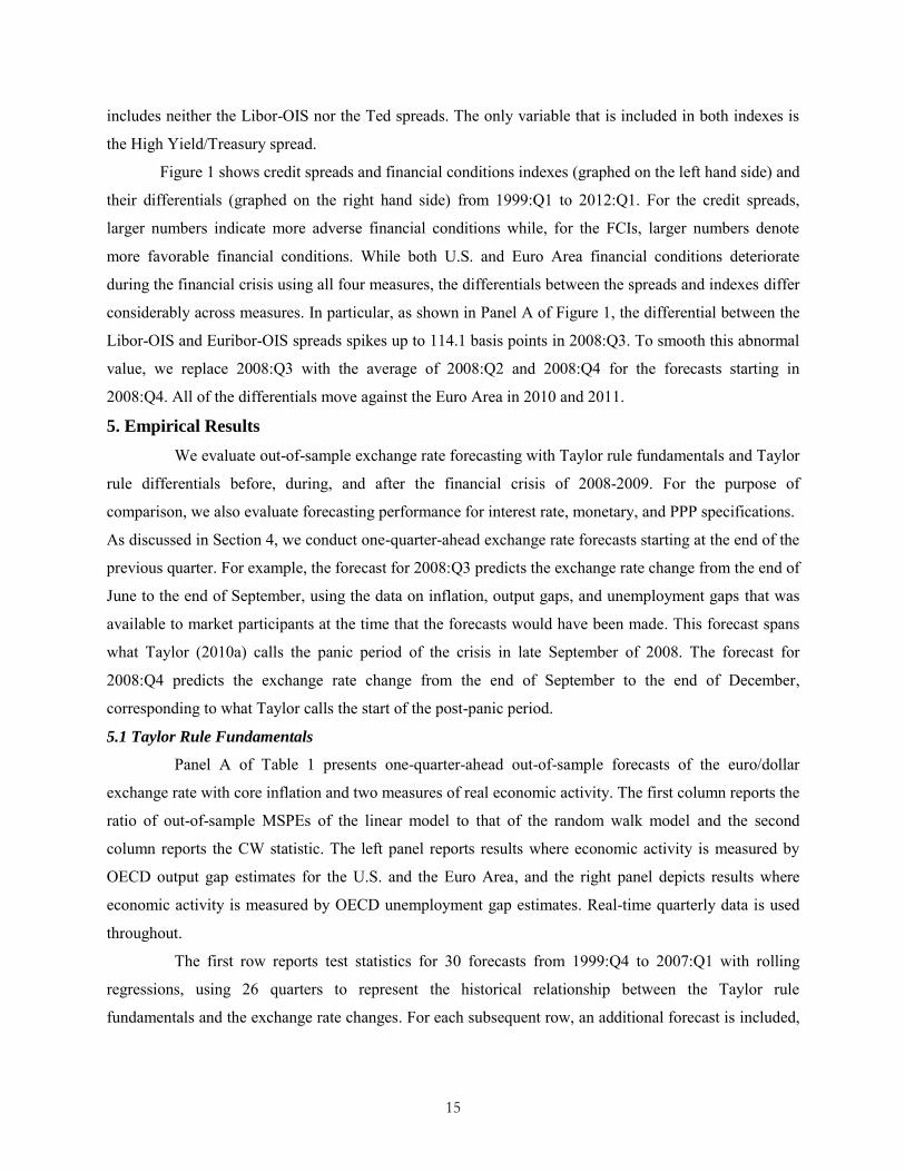
5.1 Taylor Rule Fundamentals

Panel A of Table 1 presents one-quarter-ahead out-of-sample forecasts of the euro/dollar

exchange rate with core inflation and two measures of real economic activity. The first column reports the

ratio of out-of-sample MSPEs of the linear model to that of the random walk model and the second

column reports the CW statistic. The left panel reports results where economic activity is measured by

OECD output gap estimates for the U.S. and the Euro Area, and the right panel depicts results where

economic activity is measured by OECD unemployment gap estimates. Real-time quarterly data is used

throughout.

The first row reports test statistics for 30 forecasts from 1999:Q4 to 2007:Q1 with rolling

regressions, using 26 quarters to represent the historical relationship between the Taylor rule

fundamentals and the exchange rate changes. For each subsequent row, an additional forecast is included,

16

so that the last row for 2012:Q1 reports statistics for 50 forecasts, but the rolling regressions still use 26

quarters to represent the historical relationship.

The MSPE ratios for the specification with the unemployment gap start under one with

forecasts through 2007:Q1, so the forecast errors of the linear model are smaller than those of the random

walk model, and remain under one until 2010:Q2. Under the null hypothesis of a random walk, the MSPE

of the linear model will be greater than the MSPE of the random walk model, so this represents favorable

evidence for the Taylor rule model. The no predictability null can be rejected using the CW test at the 5

percent level for the forecasts ending in 2007:Q1 and 2007:Q2, at the 1 percent level for the forecasts

ending in 2007:Q3 through 2008:Q4, and at a mix of 5 percent and 1 percent levels thereafter. The results

are not as successful for the specification with the output gap. While the no predictability null can be

rejected at the 5 or 10 percent level for the forecasts ending in 2007:Q1 through 2008:Q2, the null cannot

thereafter be rejected at the 10 percent level. The MSPE ratios are below one until 2008:Q2 and above

one thereafter.

Some intuition for these results can be found in Panel A of Figure 2, which depicts actual and

forecasted exchange rate changes with the output and unemployment gaps. Since the exchange rate is

defined as dollars per euro, observations above the zero line represent dollar depreciation, while

observations below the zero line represent dollar appreciation. The dollar steadily depreciated against the

euro from 2006:Q1 to 2008:Q1. In 2008:Q2, the depreciation turned to appreciation and, in 2008:Q3, the

dollar sharply appreciated at the peak of the financial crisis. The dollar/euro rate has remained very

volatile, with the largest appreciation in 2010:Q2 and the largest depreciation in 2010:Q3.

The forecasts with the unemployment gap track the actual exchange rate movements very well

(albeit by the low standards of out-of-sample exchange rate forecasting) through 2008:Q2. The largest

quarterly movement in the dollar/euro rate since 2000 occurred in 2008:Q3, when the dollar appreciated

by more than 10 percent. As shown in Figure 2, the Taylor rule specifications predicted continued dollar

depreciation while, by definition, the random walk model predicted neither depreciation nor appreciation.

Starting in 2009, the Taylor rule model continued to predict dollar depreciation, while the actual exchange

rate seesawed between appreciation and depreciation. For the specification with the output gap, the

forecasts were less successful through 2007. The model generally predicted dollar appreciation during

2009 and 2010 and dollar depreciation in 2011.26

5.2 Taylor Rule Differentials

Following Engel, Mark, and West (2008), we evaluate out-of-sample performance of the

Taylor rule differentials model. The results for the Taylor rule differentials model are not as strong as

26 The signs of the estimated coefficients in the forecasting regressions (not reported) are generally in accord with Equations (5) and (9), although they are usually not significant.

17

those for the Taylor rule fundamentals model. Panel B of Table 1 presents one-quarter-ahead out-of-

sample forecasts of the euro/dollar exchange rate with core inflation and both measures of economic

activity. The MSPE ratio is below one and the random walk null can be rejected at the 10 percent level in

favor of the Taylor rule differentials model for the initial sample ending in 2007:Q1 when real economic

activity is measured by either the output gap or the unemployment gap. The MSPE ratios fall during the

early part of the sample through 2008:Q1, rise during the financial crisis through 2009:Q1, and stabilize

after the crisis. The evidence of predictability is stronger with the output gap than with the unemployment

gap. With the output gap, the no predictability null can be rejected at the 10 percent level or higher for

almost all forecasts through 2009:Q4 and at the 5 percent level or higher from 2007:Q3 through 2008:Q2.

With the unemployment gap, the null can only be rejected at the 10 percent level or higher through

2008:Q2. The actual and predicted exchange rate changes are illustrated in Panel B of Figure 2. The

predicted changes are similar to those with the Taylor rule fundamentals model. The models track the

actual changes better than the random walk through 2008:Q2, incorrectly predict dollar depreciation from

2008:Q3 to 2009:Q1, and are mixed thereafter.

5.3 Credit Spreads

The results of out-of-sample Dollar/Euro exchange rate forecasts when the variables that enter

the Taylor rule specifications, inflation and output/unemployment gap differentials, are augmented by

either the Libor-OIS/Euribor-OIS differential or the U.S./Euro Area Ted spread differential are reported

in Tables 2 and 3. Panel A reports the MSPE ratios and CW statistics for the Taylor rule fundamentals

model and Panel B reports the results for the Taylor rule differentials model.

The relative performance among the specifications is similar for the models with credit spreads

as for the original models. The Taylor rule fundamentals model with the unemployment gap outperforms

the Taylor rule fundamentals model with the output gap and the Taylor rule differentials model with the

output gap outperforms the Taylor rule differentials model with the unemployment gap, and so the two

best performing specifications are the Taylor rule fundamentals model with the unemployment gap and

the Taylor rule differentials model with the output gap.

With the Libor-OIS/Euribor-OIS differential augmented Taylor rule fundamentals model with

the unemployment gap, the no predictability null hypothesis can be rejected at the 1 percent significance

level for the forecasts ending in 2007:Q1 through 2008:Q2, at the 5 percent level for the forecasts ending

in 2008:Q3 through 2009:Q1, at the 10 percent level for the forecasts ending in 2009:Q2 through

2010:Q2, and cannot be rejected thereafter. The MSPE ratios are below one from 2007:Q1 to 2008:Q2.

The next most successful results are for the Taylor rule differentials model with the output gap, where the

MSPE ratios are below one from 2007:Q1 to 2008:Q4 and the null is rejected at the 10 percent level or

higher from 2007:Q1 through 2009:Q4. Thereafter, the MSPE ratios rise and the significance level of the

18

rejections falls. For the fundamentals model with the output gap and the differentials model with the

unemployment gap, the null can only be rejected through 2008:Q2.

The results are similar when the models are augmented by the U.S./Euro Area Ted spread

differential. For the Taylor rule fundamentals model with the unemployment gap, the no predictability

null hypothesis can be rejected at the 1 percent significance level for all forecasts ending in 2007:Q1

through 2008:Q2 and at the 5 percent level for almost all forecasts ending in 2008:Q3 through 2010:Q2,

with several rejections at the 10 percent level thereafter. For the Taylor rule differentials model with the

output gap, the null can be rejected at the 1 percent level for almost all forecasts ending in 2007:Q1

through 2008:Q2 and at the 5 and 10 percent levels for the forecasts ending in 2008:Q3 through 2010:Q2.

For the fundamentals model with the output gap and the differentials model with the unemployment gap,

the null can only be rejected through 2008:Q2.

Actual and predicted exchange rate changes for the models augmented by credit spreads are

illustrated in Panel A of Figure 3. In order to conserve space, the results are depicted only for one of the

most successful specification, the Taylor rule fundamentals model with the unemployment gap. Because

of the limited span of the credit spread data, the predicted exchange rate changes with and without the

spreads are the same through 2005:Q3. Thereafter, the augmented models with the spreads show much

more variability than the original models without the spreads.

5.4 Financial Conditions Indexes

The results of out-of-sample exchange rate forecasts when the Taylor rule specifications are

augmented by either the Bloomberg FCI differentials or the OECD FCI differentials are reported in

Tables 4 and 5. Panel A reports the MSPE ratios and CW statistics for the Taylor rule fundamentals

model and Panel B reports the results for the Taylor rule differentials model.

The relative performance among the specifications with the OECD FCI differential is similar to

the original models and the models with credit spreads. The Taylor rule fundamentals model with the

unemployment gap outperforms the fundamentals model with the output gap, the Taylor rule differentials

model with the output gap outperforms the differentials model with the unemployment gap, and the best

performing specification is the Taylor rule fundamentals model with the unemployment gap. The relative

performance is more balanced across specifications for the models augmented with the Bloomberg FCI.

The most consistent evidence across specifications of out-of-sample exchange rate

predictability is obtained using the models augmented by the Bloomberg FCI differential. Using the

Taylor rule differentials model with the output gap, the no predictability null hypothesis can be rejected at

the 5 percent significance level or higher for almost all of the forecasts ending in 2007:Q1 through

2010:Q4 and at the 10 percent level for the forecasts ending in 2011:Q3 through 2012:Q1. For the Taylor

rules fundamentals model with either the output or the unemployment gap, the null can be rejected at the

19

1 percent level for all forecasts ending in 2007:Q1 through 2008:Q2 and at the 10 percent level or higher

for virtually all forecasts ending in 2008:Q3 through 2010:Q4 while, for the differentials model with the

unemployment gap, the null can be rejected at the 5 percent level from 2007:Q1 through 2008:Q4.

The results are less consistent when the models are augmented by the OECD FCI differential.

For the Taylor rule fundamentals model with the unemployment gap, the no predictability null hypothesis

can be rejected at the 1 percent significance level for the forecasts ending in 2007:Q1 through 2008:Q3,

and at the 5 percent level for almost all forecasts ending in 2008:Q4 through 2012:Q1. For the Taylor rule

differentials model with the output gap, the null is rejected at the 10 percent level or higher for almost all

of the forecasts from 2007:Q1 through 2012:Q1. The results are weaker for the Taylor rule differentials

model with the unemployment gap, where the null is rejected at the 10 percent significance level or higher

for the forecasts ending in 2007:Q1 through 2009:Q4. The weakest results are for the Taylor rule

fundamentals model with the output gap, where the null is only rejected for the forecasts ending in

2007:Q1 through 2008:Q2. The more consistent rejections using the Bloomberg FCI over the OECD FCI

are consistent with the results of Hatzius et al. (2010), who find that the Bloomberg FCI outperforms the

OECD FCI for out-of-sample prediction of four measures of real economic activity since 2005.

Actual and predicted exchange rate changes for the models augmented by FCIs are illustrated

in Panel B of Figure 3. As with the credit spreads, the results are depicted only for the Taylor rule

fundamentals model with the unemployment gap and the predicted exchange rate changes with and

without the spreads are the same through 2005:Q3. Thereafter, the augmented models with the FCIs also

show much more variability than the original models without the FCIs.

5.5 Original Versus Augmented Taylor Rule Models

We have provided evidence that the null hypothesis of no out-of-sample predictability for the

Dollar/Euro exchange rate can be rejected, although not consistently, using the original Taylor rule

model, two Taylor rule models augmented by credit spreads, and two Taylor rule models augmented by

FCIs. We now investigate whether the original Taylor rule model can be rejected against the four

augmented models on the basis of their out-of sample exchange rate forecasts. Since the Taylor rule

fundamentals model with the unemployment gap and the Taylor rule differentials model with the output

gap had the best performance against the random walk null, we will only consider those two models for

the comparison.

The MSPE ratios and CW statistics for tests with the original Taylor rule fundamentals model

with the unemployment gap as the null and the augmented fundamentals models as the alternative are

presented in Table 6. The results are very consistent across the models. The MSPE ratios are below one

and the original model null can be rejected in favor of the augmented model alternative at the 5 percent

significance level for virtually all forecasts ending in 2007:Q1 through 2008:Q2 for both spreads and

20

FCIs. For the forecasts ending in 2008:Q3 through 2012:Q2, the MSPE ratios are almost all above one

and the null hypothesis is almost never rejected. The superior performance of the models augmented by

credit spreads and FCIs prior to the panic phase of the financial crisis is consistent with the proposals,

discussed in the Introduction, to augment the Taylor rule as financial conditions worsened in 2007 and

early 2008.

The tests with the original Taylor rule differentials model with the output gap as the null and

the augmented differentials models as the alternative are presented in Table 7. While there are some

rejections for the Ted spread, Bloomberg FCI, and OECD FCI differentials, they are neither particularly

strong nor consistent across forecasts. It is not completely clear to us how these results should be

evaluated. In Tables 1 – 5, where the null hypothesis was a random walk, the tests perform very well. The

null hypothesis was rejected at the 5 percent level or higher in every case where the MSPE ratio was

below one as well as in some cases where the MSPE ratio was greater than one. In Table 7, where the null

hypothesis is not a random walk, the tests did not perform as well.27 There are a number of cases where

the MSPE ratio is below one and the null is not rejected at the 10 percent level, as well as a few cases

where the MSPE ratio is above one and the null is rejected. Given the small size of our sample, it is not

clear how applicable are the size and power results in Clark and West (2007). If we adopt a less formal

metric and say that we find evidence in favor of the augmented model if either the MSPE ratio is below

one or the CW statistic is significant at the 10 percent level, then the results are for the Taylor rule

differentials model with the output gap clearer. The model augmented with the Ted spread differentials

consistently outperforms the original model, the models augmented with the Bloomberg and OECD FCI

differentials usually outperform the original model, while the model augmented with the Libor-

OIS/Euribor-OIS FCI differentials does not usually outperform the original model.

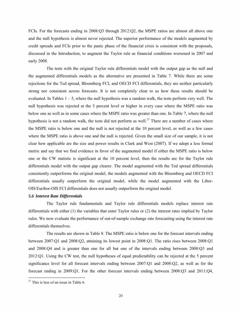
5.6 Interest Rate Differentials

The Taylor rule fundamentals and Taylor rule differentials models replace interest rate

differentials with either (1) the variables that enter Taylor rules or (2) the interest rates implied by Taylor

rules. We now evaluate the performance of out-of-sample exchange rate forecasting using the interest rate

differentials themselves.

The results are shown in Table 8. The MSPE ratio is below one for the forecast intervals ending

between 2007:Q1 and 2008:Q2, attaining its lowest point in 2008:Q1. The ratio rises between 2008:Q1

and 2008:Q4 and is greater than one for all but one of the intervals ending between 2008:Q3 and

2012:Q1. Using the CW test, the null hypotheses of equal predictability can be rejected at the 5 percent

significance level for all forecast intervals ending between 2007:Q1 and 2008:Q2, as well as for the

forecast ending in 2009:Q1. For the other forecast intervals ending between 2008:Q3 and 2011:Q4, 27 This is less of an issue in Table 6.

21

however, the equal predictability null cannot be rejected at even the 10 percent significance level. For the

forecast interval ending in 2012:Q1, the null can be rejected at the 10 percent level.

Figure 4 illustrates the results. While the fit between the actual and predicted changes in the

exchange rate are visually comparable to those from the Taylor rule models through 2006, the interest rate

differentials model is slower to pick up the subsequent appreciation of the euro and performs worse than

the others thereafter. The ECB raised its policy rate above 1 percent in 2011:Q3 and 2011:Q4. As

depicted in Figure 4, this led to actual and predicted Euro dollar depreciation in 2012:Q1, which may

account for the revival of predictability.

Prior to the panic phase of the financial crisis, the interest rate differentials model perform

about as well as either the Taylor rule fundamentals or the Taylor rule differentials models. This should

not be surprising, as this period was the heyday of the carry trade. Once the financial crisis hit and the Fed

and ECB lowered interest rates to unprecedented levels for an extended period, both Taylor rule models

outperform the interest rate model.

5.7 Monetary and PPP Fundamentals

The attainment of the zero lower bound for the federal funds rate for the U.S. in late 2008, the

sharp fall of the money market rate for the Euro Area in early 2009, and quantitative easing for the U.S.

starting in 2009 raises the question of whether more conventional specifications, with monetary or PPP

fundamentals, might replace the interest rate differentials and Taylor rule models for out-of-sample

exchange rate forecasting.

Table 8 reports one-quarter-ahead out-of-sample forecasts of the euro/dollar exchange rate with

monetary and PPP fundamentals using the same statistics that were used to evaluate the Taylor rule and

interest rate differential models. Results for the monetary model are presented with k equal to 0 and 1.

The results for the monetary and PPP models are extremely clear. For all forecast intervals and all

specifications, the MSPE ratios are greater than one and the null hypothesis of equal predictability cannot

be rejected with the CW test at even the 10 percent significance level. Neither the monetary nor the PPP

models provide any evidence whatsoever against the random walk.

Figure 4 depicts actual and forecasted exchange rate changes for the monetary and PPP models.

There is very little variation in the forecasted exchange rate changes, and neither model forecasts the

depreciation of the dollar from 2002 through 2004. While the models do a little better than the random

walk starting in 2007, the improvement is not sufficient to provide any evidence of predictability.

5.8 Summary of the Results

We have reported 1344 forecast evaluations – 21 sets of forecasts with 32 models and 2 test

statistics. In order to summarize the results, Table 9 reports the number of significant CW statistics for

each model. Panels A – E depict the number of times that the random walk (no predictability) null

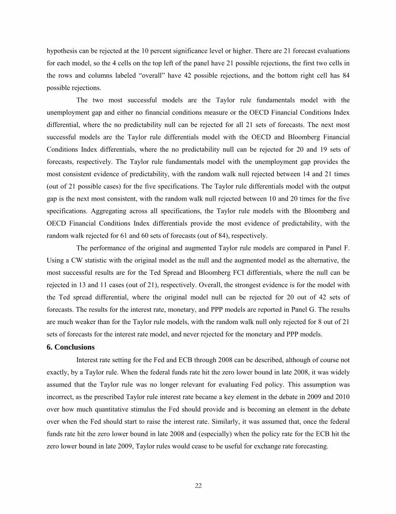
22

hypothesis can be rejected at the 10 percent significance level or higher. There are 21 forecast evaluations

for each model, so the 4 cells on the top left of the panel have 21 possible rejections, the first two cells in

the rows and columns labeled “overall” have 42 possible rejections, and the bottom right cell has 84

possible rejections.

The two most successful models are the Taylor rule fundamentals model with the

unemployment gap and either no financial conditions measure or the OECD Financial Conditions Index

differential, where the no predictability null can be rejected for all 21 sets of forecasts. The next most

successful models are the Taylor rule differentials model with the OECD and Bloomberg Financial

Conditions Index differentials, where the no predictability null can be rejected for 20 and 19 sets of

forecasts, respectively. The Taylor rule fundamentals model with the unemployment gap provides the

most consistent evidence of predictability, with the random walk null rejected between 14 and 21 times

(out of 21 possible cases) for the five specifications. The Taylor rule differentials model with the output

gap is the next most consistent, with the random walk null rejected between 10 and 20 times for the five

specifications. Aggregating across all specifications, the Taylor rule models with the Bloomberg and

OECD Financial Conditions Index differentials provide the most evidence of predictability, with the

random walk rejected for 61 and 60 sets of forecasts (out of 84), respectively.

The performance of the original and augmented Taylor rule models are compared in Panel F.

Using a CW statistic with the original model as the null and the augmented model as the alternative, the

most successful results are for the Ted Spread and Bloomberg FCI differentials, where the null can be

rejected in 13 and 11 cases (out of 21), respectively. Overall, the strongest evidence is for the model with

the Ted spread differential, where the original model null can be rejected for 20 out of 42 sets of

forecasts. The results for the interest rate, monetary, and PPP models are reported in Panel G. The results

are much weaker than for the Taylor rule models, with the random walk null only rejected for 8 out of 21

sets of forecasts for the interest rate model, and never rejected for the monetary and PPP models.

6. Conclusions

Interest rate setting for the Fed and ECB through 2008 can be described, although of course not

exactly, by a Taylor rule. When the federal funds rate hit the zero lower bound in late 2008, it was widely

assumed that the Taylor rule was no longer relevant for evaluating Fed policy. This assumption was

incorrect, as the prescribed Taylor rule interest rate became a key element in the debate in 2009 and 2010

over how much quantitative stimulus the Fed should provide and is becoming an element in the debate

over when the Fed should start to raise the interest rate. Similarly, it was assumed that, once the federal

funds rate hit the zero lower bound in late 2008 and (especially) when the policy rate for the ECB hit the

zero lower bound in late 2009, Taylor rules would cease to be useful for exchange rate forecasting.

23

In this paper, we evaluate Taylor rule based out-of-sample forecasting for the Dollar/Euro

exchange rate in an environment where one, or both, central bank policy rates are at the zero lower bound.

We use models with Taylor rule fundamentals, where the coefficients on the variables that normally

comprise Taylor rules, inflation and output/unemployment gaps, are estimated, and models with Taylor

rule differentials, where the coefficients are pre-specified. For both types of models, we also evaluate

forecasts using models that are augmented with credit spreads or financial conditions indexes.

While all of the models outperform the random walk model prior to the onset of the financial

crisis, there are large differences in performance during and after the crisis. For the original Taylor rule

models that do not incorporate financial conditions, the most successful specification is the fundamentals

model with the unemployment gap. With that specification, the models with spreads or FCIs outperform

the original model through 2008:Q2, but not thereafter. The second most successful specification is the

differentials model with the output gap. With that specification, the models with the Ted spread,

Bloomberg FCI, and OECD FCI outperform the original model.

Several of the models consistently provide evidence of predictability. The strongest evidence is

for the original Taylor rule fundamentals model, where the random walk null can be rejected for all 21

sets of forecasts at the 5 percent significance level, and for the Taylor rule fundamentals model

augmented by the OECD FCI differential, where the random walk null can be rejected for 20 out of 21

sets of forecasts at the 5 percent level (and at the 10 percent level for the 21st). Overall, the strongest

evidence is for the Taylor rule models augmented by the Bloomberg and OECD FCIs, where the random

walk null can be rejected for 61 and 60 sets of forecasts (out of 84), respectively, at the 10 percent

significance level.

The Taylor rule models are much more successful than other specifications. While the interest

rate differentials model provides some evidence of predictability through 2008:Q2, the evidence

disappears during the crisis, and the models with monetary and PPP fundamentals cannot outperform the

random walk for any sample.

Taylor rules have proven to be successful at describing interest rate setting at the Fed and other

central banks. Once policy rates hit the zero lower bound for the U.S. in late 2008 and the Euro Area in

late 2009, Taylor rules became prescriptive rather than descriptive. Measures of financial conditions have

played an important role in Taylor rule prescriptions during the financial crisis. This paper is the first (to

our knowledge) to use prescriptive Taylor rule models in order to analyze out-of-sample exchange rate

forecasting during the financial crisis. Using models with either (1) Taylor rule fundamentals and the

unemployment gap or (2) Taylor rule differentials and the output gap, we provide more evidence of out-

of-sample predictability than with the random walk benchmark, and several models that incorporate

measures of financial conditions outperform the original Taylor rule models.

24

References

Adrian, Tobias, Erkko Etula, and Hyun Song Shin, “Risk Appetite and Exchange Rates” manuscript, June 2011 Bacchetta, Philippe and Eric van Wincoop, “Infrequent Portfolio Decisions: A Solution to the Forward Discount Puzzle” American Economic Review 100, 2010, pp. 870-904 Bernanke, Ben, “Monetary Policy and the Housing Bubble”, paper delivered at the American Economic Association Meetings, January 3, 2010 Blinder, Alan S. and Ricardo Reis, “Understanding the Greenspan Standard”, in The Greenspan Era: Lessons for the Future, Federal Reserve Bank of Kansas City, 2005, pp. 11-96

Chinn, Menzie D., “Taylor Rules, Exchange Rates, and the Speculation about the Dollar/Euro Rate” [Weblog Entry], Econbrowser, http://www.econbrowser.com/archives/2008/07/taylor_rules_ex.html, 28 July 2008

__________, “Taylor Rules, Synchronized Recession and the Potential for Competitive Depreciation” [Weblog Entry], Econbrowser, http://www.econbrowser.com/archives/2008/09/taylor_rules_sy.html, 9 September 2008

__________, “ZIRP and the exchange rate...and other macro variables” [Weblog Entry], Econbrowser, 22 December 2008, http://www.econbrowser.com/archives/2008/12/zirp_and_the_ex.html, 22 December 2008 _______, “Nonlinearities, Business Cycles and Exchange Rates" Economic Notes 37, 2008, pp. 219-239 Clarida, Richard, Jordi Gali, and Mark Gertler, “Monetary Rules in Practice: Some International Evidence” European Economic Review 42, 1998, pp. 1033-1067 Clark, Todd and Kenneth D. West, “Using Out-of-Sample Mean Squared Prediction Errors to Test the Martingale Difference Hypothesis” Journal of Econometrics 135, 2006, pp. 155-186 _______, “Approximately Normal Tests for Equal Predictive Accuracy in Nested Models” Journal of Econometrics 138, 2007, pp. 291-311 Croushore, Dean and Tom Stark, “A Real-Time Data Set for Macroeconomists,” Journal of Econometrics, 105, 2001, pp. 111-130

Curdia, Vasco and Michael Woodford, “Credit Spreads and Monetary Policy”, Journal of Money, Credit and Banking 42, 2010, pp. 3-35 Diebold, Francis and Robert Mariano, “Comparing Predictive Accuracy” Journal of Business and Economic Statistics, 1995, 13, pp.253-263 Eichenbaum, Martin and Charles Evans, “Some Empirical Evidence on the Effects of Shocks to Monetary Policy on Exchange Rates” Quarterly Journal of Economics, November 1995, CX, pp. 975-1009. Engel, Charles, Nelson C. Mark, and Kenneth D. West, “Exchange Rate Models Are Not as Bad as You Think” NBER Macroeconomics Annual 2007, University of Chicago Press, 2008, pp. 381-441

25

Engel, Charles, Nelson C. Mark, and Kenneth D. West, “Factor Model Forecasts of Exchange Rates” unpublished, University of Wisconsin, January 2012 Faust, Jon and John H. Rogers, “Monetary Policy’s Role in Exchange Rate Behavior” Journal of Monetary Economics 50, 2003, pp. 1403-1424 Faust, Jon, John H. Rogers, and Jonathan H. Wright, “Exchange Rate Forecasting: the Errors We’ve Really Made” Journal of International Economics 60, 2003, pp. 35-59 Giacomini, Raffaella, and Barbara Rossi, “Forecast Comparisons in Unstable Environments,” Journal of Applied Econometrics 25, 2010, pp. 595-620. Gourinchas, Pierre-Olivier and Helene Rey, “International Financial Adjustment” Journal of Political Economy 115, 2007, pp. 665-703 Gourinchas, Pierre-Olivier and Aaron Tornell, “Exchange Rate Puzzles and Distorted Beliefs” Journal of International Economics 64, 2004, pp. 303-333 Hatzius, Jan, Peter Hooper, Frederic Mishkin, Kermit L. Schoenholtz and Mark W. Watson, “Financial Conditions Indexes: A Fresh Look after the Financial Crisis,” U.S. Monetary Policy Forum, April 2010 Ince, Onur, “Forecasting Exchange Rates Out-of-Sample with Panel Methods and Real-Time Data,” unpublished, Appalachian State University, 2012 Inoue, Atsushi and Barbara Rossi, “Out-of-Sample Forecast Tests Robust to the Window Size Choice,” unpublished, Duke University, 2011 Mark, Nelson, “Exchange Rate and Fundamentals: Evidence on Long-Horizon Predictability” American Economic Review 85, 1995, pp. 201-218 McCracken, Michael, “Asymptotics for Out-of-Sample Tests of Granger Causality” Journal of Econometrics 140, 2007, pp.719-752 McCulley, Paul and Ramin Toloui, “Chasing the Neutral Rate Down: Financial Conditions, Monetary Policy, and the Taylor Rule,” Global Central Bank Focus Pacific Investment Management Company (PIMCO), February 2008, Available at http://www.pimco.com/EN/Insights/Pages/GCBF%2002-2008.aspx Meese, Richard A. and Kenneth Rogoff, “Empirical Exchange Rate Models of the Seventies: Do They Fit Out of Sample?” Journal of International Economics 14, 1983, pp.3-24 Meyer, Laurence, “Dueling Taylor Rules,” Monetary Policy Insights, Macroeconomic Advisors, August 20, 2009 Mishkin, Frederic S., “Monetary Policy Flexibility, Risk Management, and Financial Disruptions,” Federal Reserve Bank of New York, January 11, Available at http://www.federalreserve.gov/newsevents /speech/mishkin20080111a.htm Molodtsova, Tanya and David H. Papell, “Exchange Rate Predictability with Taylor Rule Fundamentals” Journal of International Economics 77, 2009, pp. 167-180

26

Molodtsova, Tanya, Alex Nikolsko-Rzhevskyy and David H. Papell, “Taylor Rules with Real-Time Data: A Tale of Two Countries and One Exchange Rate” Journal of Monetary Economics 55, 2008, pp. S63-S79 __________, “Taylor Rules and the Euro” Journal of Money, Credit, and Banking, March-April 2011, pp. 535-552 Nikolsko-Rzhevskyy, Alex, and David H. Papell, “Taylor’s Rule versus Taylor Rules,” unpublished, University of Houston, 2011

Rogoff, Kenneth and Vania Stavrakeva, “The Continuing Puzzle of Short Horizon Exchange Rate Forecasting” National Bureau of Economic Research Working Paper 14071, 2008 Rosenberg, Michael R., Financial Conditions Watch, Bloomberg, April 13, 2012 Rudebusch, Glenn, “The Fed’s Exit Strategy for Monetary Policy” Federal Reserve Bank of San Francisco Economic Letter 18, June 14, 2010, pp. 1-5 Scholl, Almuth and Harald Uhlig, “New Evidence on the Puzzles: Results from Agnostic Identification on Monetary Policy and Exchange Rates” Journal of International Economics 76, 2008, pp. 1-13 Taylor, John B., “Discretion versus Policy Rules in Practice” Carnegie-Rochester Conference Series on Public Policy 39, 1993, pp. 195-214 _________, “The Costs and Benefits of Deviating from the Systematic Component of Monetary Policy,” Keynote Address at the Federal Reserve Bank of San Francisco Conference on “Monetary Policy and Asset Markets”, February 22, 2008 _________, “Assessing the Federal Policy Response to the Economic Crisis” Testimony before the Committee on the Budget, United States Senate, 22 September 2010, 2010a

_____________, “Policy Rule Gaps as Forecasts of Currency and Interest Rate Movements”, [Weblog Entry], Economics One, http://johnbtaylorsblog.blogspot.com/2010/09/policy-rule-gaps-as-forecasts-of.html, September 30, 2010, 2010b Taylor, John B. and John C. Williams, “A Black Swan in the Money Market” American Economic Journal: Macroeconomics 1, 2009, pp. 58-83 Thornton, Daniel, “What the Libor-OIS Spread Says,” Federal Reserve Bank of St. Louis Economic Synopses 24, May 11, 2009 Walsh, Carl E., “Using Monetary Policy to Stabilize Economic Activity”, in Financial Stability and Macroeconomic Policy, Federal Reserve Bank of Kansas City, 2010, pp. 245-296 West, Kenneth D., “Asymptotic Inference about Predictive Ability” Econometrica, 1996, 64, pp.1067-1084

27

A. LIBOR-OIS and EURIBOR-OIS Spreads

B. TED Spreads for the US and Euro Area

C. Bloomberg US and Euro Area Financial Condition Indexes

D. OECD Financial Condition Indexes for the US and Euro Area

Figure 1. Credit Spreads and Financial Stress Indexes with their Differentials

-50

0

50

100

150

200

250 Q

1-19

99

Q4-

1999

Q

3-20

00

Q2-

2001

Q

1-20

02

Q4-

2002

Q

3-20

03

Q2-

2004

Q

1-20

05

Q4-

2005

Q

3-20

06

Q2-

2007

Q

1-20

08

Q4-

2008

Q

3-20

09

Q2-

2010

Q

1-20

11

Q4-

2011

LIBOR-OIS Spread EURIBOR-OIS Spread

-100

-50

0

50

100

150

Q1-

1999

Q

4-19

99

Q3-

2000

Q

2-20

01

Q1-

2002

Q

4-20

02

Q3-

2003

Q

2-20

04

Q1-

2005

Q

4-20

05

Q3-

2006

Q

2-20

07

Q1-

2008

Q

4-20

08

Q3-

2009

Q

2-20

10

Q1-

2011

Q

4-20

11

LIBOR-OIS/EURIBOR-OIS Spread Differential

-1.0

0.0

1.0

2.0

3.0

4.0

Q1-

1999

Q

4-19

99

Q3-

2000

Q

2-20

01

Q1-

2002

Q

4-20

02

Q3-

2003

Q

2-20

04

Q1-

2005

Q

4-20

05

Q3-

2006

Q

2-20

07

Q1-

2008

Q

4-20

08

Q3-

2009

Q

2-20

10

Q1-

2011

Q

4-20

11

US TED Spread EU TED Spread

-2

-1

0

1

Q1-

1999

Q

4-19

99

Q3-

2000

Q

2-20

01

Q1-

2002

Q

4-20

02

Q3-

2003

Q

2-20

04

Q1-

2005

Q

4-20

05

Q3-

2006

Q

2-20

07

Q1-

2008

Q

4-20

08

Q3-

2009

Q

2-20

10

Q1-

2011

Q

4-20

11

US/EU TED Spread Differential

-8

-6

-4

-2

0

2

Q1-

1999

Q

4-19

99

Q3-

2000

Q

2-20

01

Q1-

2002

Q

4-20

02

Q3-

2003

Q

2-20

04

Q1-

2005

Q

4-20

05

Q3-

2006

Q

2-20

07

Q1-

2008

Q

4-20

08

Q3-

2009

Q

2-20

10

Q1-

2011

Q

4-20

11

Bloomberg US FCI Bloomberg EU FCI

-2

0

2

4

Q1-

1999

Q

4-19

99

Q3-

2000

Q

2-20

01

Q1-

2002

Q

4-20

02

Q3-

2003

Q

2-20

04

Q1-

2005

Q

4-20

05

Q3-

2006

Q

2-20

07

Q1-

2008

Q

4-20

08

Q3-

2009

Q

2-20

10

Q1-

2011

Q

4-20

11

US/EU Bloomberg FCI Differential

-6

-4

-2

0

2

4

Q1-

1999

Q

4-19

99

Q3-

2000

Q

2-20

01

Q1-

2002

Q

4-20

02

Q3-

2003

Q

2-20

04

Q1-

2005

Q

4-20

05

Q3-

2006

Q

2-20

07

Q1-

2008

Q

4-20

08

Q3-

2009

Q

2-20

10

Q1-

2011

Q

4-20

11

OECD US FCI OECD EU FCI

-4

-2

0

2

4

Q1-

1999

Q

4-19

99

Q3-

2000

Q

2-20

01

Q1-

2002

Q

4-20

02

Q3-

2003

Q

2-20

04

Q1-

2005

Q

4-20

05

Q3-

2006

Q

2-20

07

Q1-

2008

Q

4-20

08

Q3-

2009

Q

2-20

10

Q1-

2011

Q

4-20

11

US/EU OECD FCI Differential

28

OECD Output Gap Unemployment Gap

A. Taylor Rule Fundamentals Model

OECD Output Gap Unemployment Gap

B. Taylor Rule Differentials Model

Figure 2. Actual and Predicted Changes in the Dollar/Euro Exchange Rate

-15

-10

-5

0

5

10

15 Q

4-19

99

Q3-

2000

Q

2-20

01

Q1-

2002

Q

4-20

02

Q3-

2003

Q

2-20

04

Q1-

2005

Q

4-20

05

Q3-

2006

Q

2-20

07

Q1-

2008

Q

4-20

08

Q3-

2009

Q

2-20

10

Q1-

2011

Q

4-20

11

actual predicted -15

-10

-5

0

5

10

15

Q4-

1999

Q

3-20

00

Q2-

2001

Q

1-20

02

Q4-

2002

Q

3-20

03

Q2-

2004

Q

1-20

05

Q4-

2005

Q

3-20

06

Q2-

2007

Q

1-20

08

Q4-

2008

Q

3-20

09

Q2-

2010

Q

1-20

11

Q4-

2011

actual predicted

-15

-10

-5

0

5

10

15

Q4-

1999

Q

3-20

00

Q2-

2001

Q

1-20

02

Q4-

2002

Q

3-20

03

Q2-

2004

Q

1-20

05

Q4-

2005

Q

3-20

06

Q2-

2007

Q

1-20

08

Q4-

2008

Q

3-20

09

Q2-

2010

Q

1-20

11

Q4-

2011

actual predicted -15

-10

-5

0

5

10

15 Q

4-19

99

Q3-

2000

Q

2-20

01

Q1-

2002

Q

4-20

02

Q3-

2003

Q

2-20

04

Q1-

2005

Q

4-20

05

Q3-

2006

Q

2-20

07

Q1-

2008

Q

4-20

08

Q3-

2009

Q

2-20

10

Q1-

2011

Q

4-20

11

actual predicted

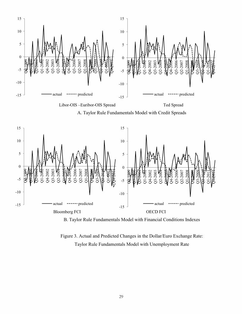
29

Libor-OIS –Euribor-OIS Spread Ted Spread

A. Taylor Rule Fundamentals Model with Credit Spreads

Bloomberg FCI OECD FCI

B. Taylor Rule Fundamentals Model with Financial Conditions Indexes

Figure 3. Actual and Predicted Changes in the Dollar/Euro Exchange Rate:

Taylor Rule Fundamentals Model with Unemployment Rate

-15

-10

-5

0

5

10

15

Q4-

1999

Q

3-20

00

Q2-

2001

Q

1-20

02

Q4-

2002

Q

3-20

03

Q2-

2004

Q

1-20

05

Q4-

2005

Q

3-20

06

Q2-

2007

Q

1-20

08

Q4-

2008

Q

3-20

09

Q2-

2010

Q

1-20

11

Q4-

2011

actual predicted -15

-10

-5

0

5

10

15

Q4-

1999

Q

3-20

00

Q2-

2001

Q

1-20

02

Q4-

2002

Q

3-20

03

Q2-

2004

Q

1-20

05

Q4-

2005

Q

3-20

06

Q2-

2007

Q

1-20

08

Q4-

2008

Q

3-20

09

Q2-

2010

Q

1-20

11

Q4-

2011

actual predicted

-15

-10

-5

0

5

10

15

Q4-

1999

Q

3-20

00

Q2-

2001

Q

1-20

02

Q4-

2002

Q

3-20

03

Q2-

2004

Q

1-20

05

Q4-

2005

Q

3-20

06

Q2-

2007

Q

1-20

08

Q4-

2008

Q

3-20

09

Q2-

2010

Q

1-20

11

Q4-

2011

actual predicted -15

-10

-5

0

5

10

15 Q

4-19

99

Q3-

2000

Q

2-20

01

Q1-

2002

Q

4-20

02

Q3-

2003

Q

2-20

04

Q1-

2005

Q

4-20

05

Q3-

2006

Q

2-20

07

Q1-

2008

Q

4-20

08

Q3-

2009

Q

2-20

10

Q1-

2011

Q

4-20

11

actual predicted

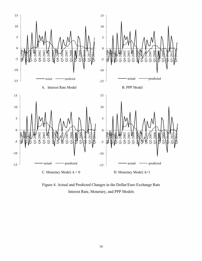
30

A. Interest Rate Model B. PPP Model

C. Monetary Model: k = 0 D. Monetary Model: k=1

Figure 4. Actual and Predicted Changes in the Dollar/Euro Exchange Rate

Interest Rate, Monetary, and PPP Models

-15

-10

-5

0

5

10

15

Q4-

1999

Q

3-20

00

Q2-

2001

Q

1-20

02

Q4-

2002

Q

3-20

03

Q2-

2004

Q

1-20

05

Q4-

2005

Q

3-20

06

Q2-

2007

Q

1-20

08

Q4-

2008

Q

3-20

09

Q2-

2010

Q

1-20

11

Q4-

2011

actual predicted -15

-10

-5

0

5

10

15

Q4-

1999

Q

3-20

00

Q2-

2001

Q

1-20

02

Q4-

2002

Q

3-20

03

Q2-

2004

Q

1-20

05

Q4-

2005

Q

3-20

06

Q2-

2007

Q

1-20

08

Q4-

2008

Q

3-20

09

Q2-

2010

Q

1-20

11

Q4-

2011

actual predicted

-15

-10

-5

0

5

10

15

Q4-

1999

Q

3-20

00

Q2-

2001

Q

1-20

02

Q4-

2002

Q

3-20

03

Q2-

2004

Q

1-20

05

Q4-

2005

Q

3-20

06

Q2-

2007

Q

1-20

08

Q4-

2008

Q

3-20

09

Q2-

2010

Q

1-20

11

Q4-

2011

actual predicted -15

-10

-5

0

5

10

15

Q4-

1999

Q

3-20

00

Q2-

2001

Q

1-20

02

Q4-

2002

Q

3-20

03

Q2-

2004

Q

1-20

05

Q4-

2005

Q

3-20

06

Q2-

2007

Q

1-20

08

Q4-

2008

Q

3-20

09

Q2-

2010

Q

1-20

11

Q4-

2011

actual predicted

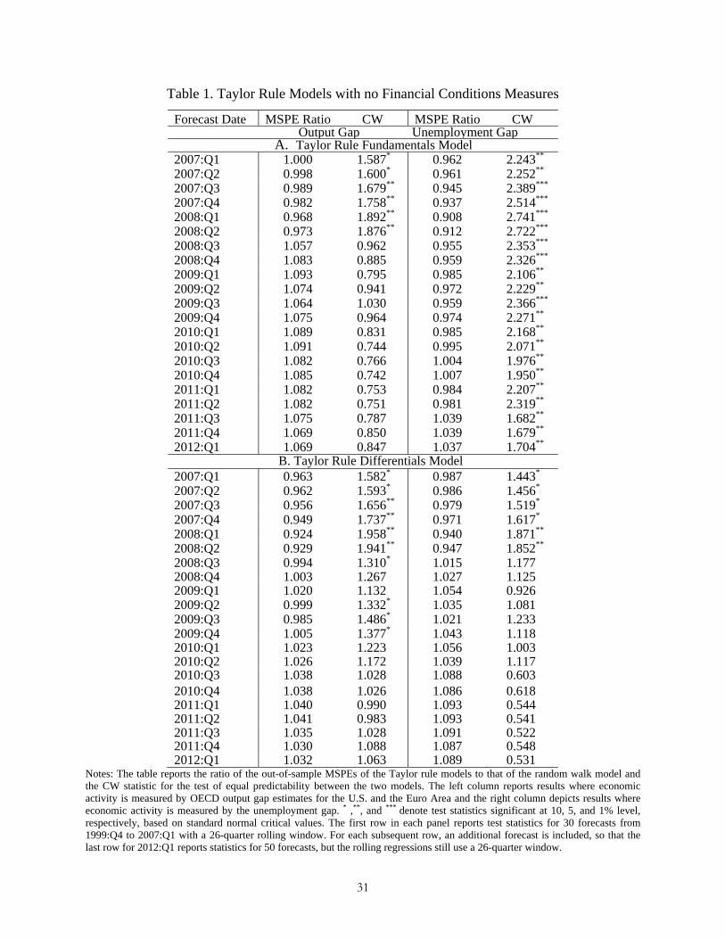
31

Table 1. Taylor Rule Models with no Financial Conditions Measures

Forecast Date MSPE Ratio CW MSPE Ratio CW Output Gap Unemployment Gap

A. Taylor Rule Fundamentals Model2007:Q1 1.000 1.587* 0.962 2.243** 2007:Q2 0.998 1.600* 0.961 2.252** 2007:Q3 0.989 1.679** 0.945 2.389*** 2007:Q4 0.982 1.758** 0.937 2.514*** 2008:Q1 0.968 1.892** 0.908 2.741*** 2008:Q2 0.973 1.876** 0.912 2.722*** 2008:Q3 1.057 0.962 0.955 2.353*** 2008:Q4 1.083 0.885 0.959 2.326*** 2009:Q1 1.093 0.795 0.985 2.106** 2009:Q2 1.074 0.941 0.972 2.229** 2009:Q3 1.064 1.030 0.959 2.366*** 2009:Q4 1.075 0.964 0.974 2.271** 2010:Q1 1.089 0.831 0.985 2.168** 2010:Q2 1.091 0.744 0.995 2.071** 2010:Q3 1.082 0.766 1.004 1.976** 2010:Q4 1.085 0.742 1.007 1.950** 2011:Q1 1.082 0.753 0.984 2.207** 2011:Q2 1.082 0.751 0.981 2.319** 2011:Q3 1.075 0.787 1.039 1.682** 2011:Q4 1.069 0.850 1.039 1.679** 2012:Q1 1.069 0.847 1.037 1.704** B. Taylor Rule Differentials Model2007:Q1 0.963 1.582* 0.987 1.443* 2007:Q2 0.962 1.593* 0.986 1.456* 2007:Q3 0.956 1.656** 0.979 1.519* 2007:Q4 0.949 1.737** 0.971 1.617* 2008:Q1 0.924 1.958** 0.940 1.871** 2008:Q2 0.929 1.941** 0.947 1.852** 2008:Q3 0.994 1.310* 1.015 1.177 2008:Q4 1.003 1.267 1.027 1.125 2009:Q1 1.020 1.132 1.054 0.926 2009:Q2 0.999 1.332* 1.035 1.081 2009:Q3 0.985 1.486* 1.021 1.233 2009:Q4 1.005 1.377* 1.043 1.118 2010:Q1 1.023 1.223 1.056 1.003 2010:Q2 1.026 1.172 1.039 1.117 2010:Q3 1.038 1.028 1.088 0.603 2010:Q4 1.038 1.026 1.086 0.618 2011:Q1 1.040 0.990 1.093 0.544 2011:Q2 1.041 0.983 1.093 0.541 2011:Q3 1.035 1.028 1.091 0.522 2011:Q4 1.030 1.088 1.087 0.548 2012:Q1 1.032 1.063 1.089 0.531

Notes: The table reports the ratio of the out-of-sample MSPEs of the Taylor rule models to that of the random walk model and the CW statistic for the test of equal predictability between the two models. The left column reports results where economic activity is measured by OECD output gap estimates for the U.S. and the Euro Area and the right column depicts results where economic activity is measured by the unemployment gap. * ,**, and *** denote test statistics significant at 10, 5, and 1% level, respectively, based on standard normal critical values. The first row in each panel reports test statistics for 30 forecasts from 1999:Q4 to 2007:Q1 with a 26-quarter rolling window. For each subsequent row, an additional forecast is included, so that the last row for 2012:Q1 reports statistics for 50 forecasts, but the rolling regressions still use a 26-quarter window.

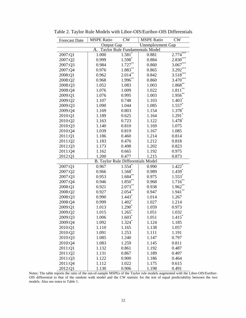
32

Table 2. Taylor Rule Models with Libor-OIS/Euribor-OIS Differentials

Forecast Date MSPE Ratio CW MSPE Ratio CW Output Gap Unemployment Gap

A. Taylor Rule Fundamentals Model2007:Q1 1.000 1.581* 0.881 2.774*** 2007:Q2 0.999 1.598* 0.884 2.830*** 2007:Q3 0.984 1.727** 0.860 3.067*** 2007:Q4 0.976 1.883** 0.865 3.292*** 2008:Q1 0.962 2.014** 0.842 3.518*** 2008:Q2 0.968 1.996** 0.860 3.470*** 2008:Q3 1.052 1.083 1.003 1.868** 2008:Q4 1.076 1.009 1.022 1.811** 2009:Q1 1.076 0.995 1.003 1.956** 2009:Q2 1.107 0.748 1.103 1.403* 2009:Q3 1.090 1.044 1.085 1.557* 2009:Q4 1.169 0.803 1.154 1.378* 2010:Q1 1.189 0.625 1.164 1.291* 2010:Q2 1.163 0.723 1.122 1.478* 2010:Q3 1.140 0.810 1.169 1.075 2010:Q4 1.039 0.819 1.167 1.085 2011:Q1 1.186 0.460 1.214 0.814 2011:Q2 1.183 0.476 1.212 0.818 2011:Q3 1.173 0.498 1.202 0.823 2011:Q4 1.162 0.665 1.192 0.975 2012:Q1 1.200 0.477 1.215 0.873

B. Taylor Rule Differentials Model2007:Q1 0.967 1.554* 0.990 1.422* 2007:Q2 0.966 1.568* 0.989 1.439* 2007:Q3 0.953 1.684** 0.975 1.553* 2007:Q4 0.946 1.850** 0.968 1.716** 2008:Q1 0.921 2.073** 0.938 1.962** 2008:Q2 0.927 2.054** 0.947 1.941** 2008:Q3 0.990 1.443* 1.014 1.267 2008:Q4 0.999 1.402* 1.027 1.214 2009:Q1 1.013 1.290* 1.059 0.973 2009:Q2 1.015 1.265* 1.051 1.032 2009:Q3 1.006 1.603* 1.051 1.415* 2009:Q4 1.092 1.324* 1.124 1.185 2010:Q1 1.110 1.165 1.138 1.057 2010:Q2 1.091 1.253 1.111 1.191 2010:Q3 1.085 1.240 1.147 0.797 2010:Q4 1.083 1.259 1.145 0.811 2011:Q1 1.132 0.861 1.192 0.487 2011:Q2 1.131 0.867 1.189 0.497 2011:Q3 1.122 0.900 1.186 0.464 2011:Q4 1.112 1.022 1.175 0.615 2012:Q1 1.130 0.906 1.198 0.491

Notes: The table reports the ratio of the out-of-sample MSPEs of the Taylor rule models augmented with the Libor-OIS/Euribor-OIS differential to that of the random walk model and the CW statistic for the test of equal predictability between the two models. Also see notes to Table 1.

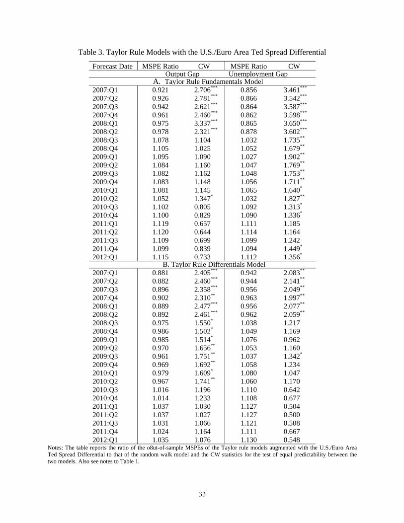
33

Table 3. Taylor Rule Models with the U.S./Euro Area Ted Spread Differential

Forecast Date MSPE Ratio CW MSPE Ratio CW Output Gap Unemployment Gap A. Taylor Rule Fundamentals Model

2007:Q1 0.921 2.706*** 0.856 3.461*** 2007:Q2 0.926 2.781*** 0.866 3.542*** 2007:Q3 0.942 2.621*** 0.864 3.587*** 2007:Q4 0.961 2.460*** 0.862 3.598*** 2008:Q1 0.975 3.337*** 0.865 3.650*** 2008:Q2 0.978 2.321*** 0.878 3.602*** 2008:Q3 1.078 1.104 1.032 1.735** 2008:Q4 1.105 1.025 1.052 1.679** 2009:Q1 1.095 1.090 1.027 1.902** 2009:Q2 1.084 1.160 1.047 1.769** 2009:Q3 1.082 1.162 1.048 1.753** 2009:Q4 1.083 1.148 1.056 1.711** 2010:Q1 1.081 1.145 1.065 1.640* 2010:Q2 1.052 1.347* 1.032 1.827** 2010:Q3 1.102 0.805 1.092 1.313* 2010:Q4 1.100 0.829 1.090 1.336* 2011:Q1 1.119 0.657 1.111 1.185 2011:Q2 1.120 0.644 1.114 1.164 2011:Q3 1.109 0.699 1.099 1.242 2011:Q4 1.099 0.839 1.094 1.449* 2012:Q1 1.115 0.733 1.112 1.356*

B. Taylor Rule Differentials Model2007:Q1 0.881 2.405*** 0.942 2.083** 2007:Q2 0.882 2.460*** 0.944 2.141** 2007:Q3 0.896 2.358*** 0.956 2.049** 2007:Q4 0.902 2.310** 0.963 1.997** 2008:Q1 0.889 2.477*** 0.956 2.077** 2008:Q2 0.892 2.461*** 0.962 2.059** 2008:Q3 0.975 1.550* 1.038 1.217 2008:Q4 0.986 1.502* 1.049 1.169 2009:Q1 0.985 1.514* 1.076 0.962 2009:Q2 0.970 1.656** 1.053 1.160 2009:Q3 0.961 1.751** 1.037 1.342* 2009:Q4 0.969 1.692** 1.058 1.234 2010:Q1 0.979 1.609* 1.080 1.047 2010:Q2 0.967 1.741** 1.060 1.170 2010:Q3 1.016 1.196 1.110 0.642 2010:Q4 1.014 1.233 1.108 0.677 2011:Q1 1.037 1.030 1.127 0.504 2011:Q2 1.037 1.027 1.127 0.500 2011:Q3 1.031 1.066 1.121 0.508 2011:Q4 1.024 1.164 1.111 0.667 2012:Q1 1.035 1.076 1.130 0.548

Notes: The table reports the ratio of the o8ut-of-sample MSPEs of the Taylor rule models augmented with the U.S./Euro Area Ted Spread Differential to that of the random walk model and the CW statistics for the test of equal predictability between the two models. Also see notes to Table 1.

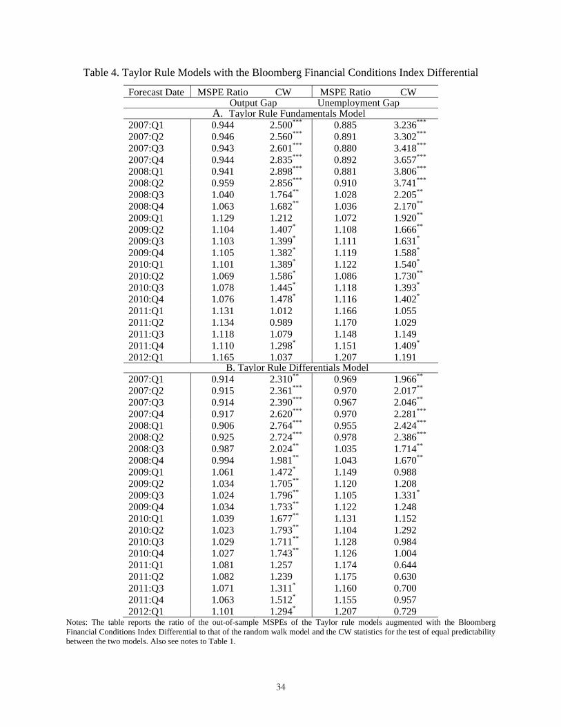
34

Table 4. Taylor Rule Models with the Bloomberg Financial Conditions Index Differential

Forecast Date MSPE Ratio CW MSPE Ratio CW Output Gap Unemployment Gap A. Taylor Rule Fundamentals Model

2007:Q1 0.944 2.500*** 0.885 3.236*** 2007:Q2 0.946 2.560*** 0.891 3.302*** 2007:Q3 0.943 2.601*** 0.880 3.418*** 2007:Q4 0.944 2.835*** 0.892 3.657*** 2008:Q1 0.941 2.898*** 0.881 3.806*** 2008:Q2 0.959 2.856*** 0.910 3.741*** 2008:Q3 1.040 1.764** 1.028 2.205** 2008:Q4 1.063 1.682** 1.036 2.170** 2009:Q1 1.129 1.212 1.072 1.920** 2009:Q2 1.104 1.407* 1.108 1.666** 2009:Q3 1.103 1.399* 1.111 1.631* 2009:Q4 1.105 1.382* 1.119 1.588* 2010:Q1 1.101 1.389* 1.122 1.540* 2010:Q2 1.069 1.586* 1.086 1.730** 2010:Q3 1.078 1.445* 1.118 1.393* 2010:Q4 1.076 1.478* 1.116 1.402* 2011:Q1 1.131 1.012 1.166 1.055 2011:Q2 1.134 0.989 1.170 1.029 2011:Q3 1.118 1.079 1.148 1.149 2011:Q4 1.110 1.298* 1.151 1.409* 2012:Q1 1.165 1.037 1.207 1.191

B. Taylor Rule Differentials Model2007:Q1 0.914 2.310** 0.969 1.966** 2007:Q2 0.915 2.361*** 0.970 2.017** 2007:Q3 0.914 2.390*** 0.967 2.046** 2007:Q4 0.917 2.620*** 0.970 2.281*** 2008:Q1 0.906 2.764*** 0.955 2.424*** 2008:Q2 0.925 2.724*** 0.978 2.386*** 2008:Q3 0.987 2.024** 1.035 1.714** 2008:Q4 0.994 1.981** 1.043 1.670** 2009:Q1 1.061 1.472* 1.149 0.988 2009:Q2 1.034 1.705** 1.120 1.208 2009:Q3 1.024 1.796** 1.105 1.331* 2009:Q4 1.034 1.733** 1.122 1.248 2010:Q1 1.039 1.677** 1.131 1.152 2010:Q2 1.023 1.793** 1.104 1.292 2010:Q3 1.029 1.711** 1.128 0.984 2010:Q4 1.027 1.743** 1.126 1.004 2011:Q1 1.081 1.257 1.174 0.644 2011:Q2 1.082 1.239 1.175 0.630 2011:Q3 1.071 1.311* 1.160 0.700 2011:Q4 1.063 1.512* 1.155 0.957 2012:Q1 1.101 1.294* 1.207 0.729

Notes: The table reports the ratio of the out-of-sample MSPEs of the Taylor rule models augmented with the Bloomberg Financial Conditions Index Differential to that of the random walk model and the CW statistics for the test of equal predictability between the two models. Also see notes to Table 1.

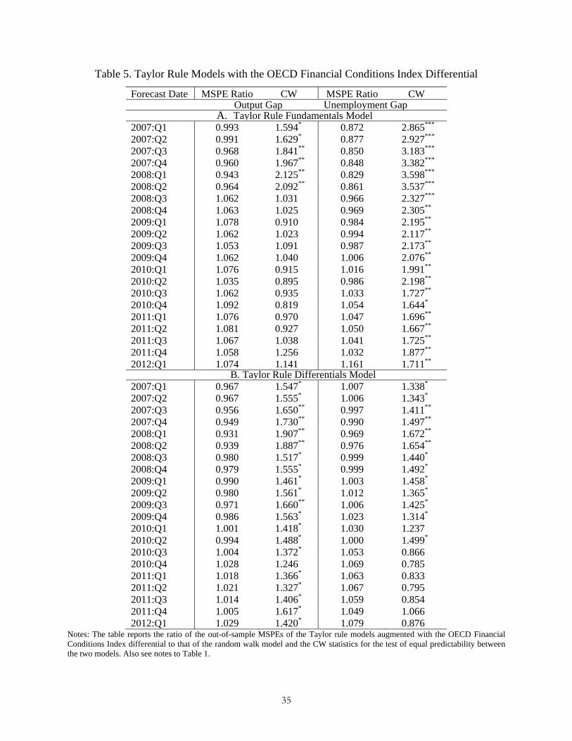
35

Table 5. Taylor Rule Models with the OECD Financial Conditions Index Differential

Forecast Date MSPE Ratio CW MSPE Ratio CW Output Gap Unemployment Gap A. Taylor Rule Fundamentals Model

2007:Q1 0.993 1.594* 0.872 2.865*** 2007:Q2 0.991 1.629* 0.877 2.927*** 2007:Q3 0.968 1.841** 0.850 3.183*** 2007:Q4 0.960 1.967** 0.848 3.382*** 2008:Q1 0.943 2.125** 0.829 3.598*** 2008:Q2 0.964 2.092** 0.861 3.537*** 2008:Q3 1.062 1.031 0.966 2.327*** 2008:Q4 1.063 1.025 0.969 2.305** 2009:Q1 1.078 0.910 0.984 2.195** 2009:Q2 1.062 1.023 0.994 2.117** 2009:Q3 1.053 1.091 0.987 2.173** 2009:Q4 1.062 1.040 1.006 2.076** 2010:Q1 1.076 0.915 1.016 1.991** 2010:Q2 1.035 0.895 0.986 2.198** 2010:Q3 1.062 0.935 1.033 1.727** 2010:Q4 1.092 0.819 1.054 1.644* 2011:Q1 1.076 0.970 1.047 1.696** 2011:Q2 1.081 0.927 1.050 1.667** 2011:Q3 1.067 1.038 1.041 1.725** 2011:Q4 1.058 1.256 1.032 1.877** 2012:Q1 1.074 1.141 1.161 1.711**

B. Taylor Rule Differentials Model2007:Q1 0.967 1.547* 1.007 1.338* 2007:Q2 0.967 1.555* 1.006 1.343* 2007:Q3 0.956 1.650** 0.997 1.411** 2007:Q4 0.949 1.730** 0.990 1.497** 2008:Q1 0.931 1.907** 0.969 1.672** 2008:Q2 0.939 1.887** 0.976 1.654** 2008:Q3 0.980 1.517* 0.999 1.440* 2008:Q4 0.979 1.555* 0.999 1.492* 2009:Q1 0.990 1.461* 1.003 1.458* 2009:Q2 0.980 1.561* 1.012 1.365* 2009:Q3 0.971 1.660** 1.006 1.425* 2009:Q4 0.986 1.563* 1.023 1.314* 2010:Q1 1.001 1.418* 1.030 1.237 2010:Q2 0.994 1.488* 1.000 1.499* 2010:Q3 1.004 1.372* 1.053 0.866 2010:Q4 1.028 1.246 1.069 0.785 2011:Q1 1.018 1.366* 1.063 0.833 2011:Q2 1.021 1.327* 1.067 0.795 2011:Q3 1.014 1.406* 1.059 0.854 2011:Q4 1.005 1.617* 1.049 1.066 2012:Q1 1.029 1.420* 1.079 0.876

Notes: The table reports the ratio of the out-of-sample MSPEs of the Taylor rule models augmented with the OECD Financial Conditions Index differential to that of the random walk model and the CW statistics for the test of equal predictability between the two models. Also see notes to Table 1.

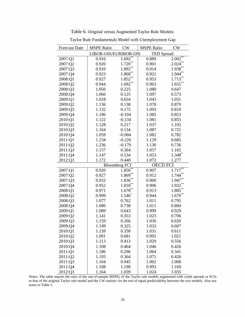
36

Table 6. Original versus Augmented Taylor Rule Models:

Taylor Rule Fundamentals Model with Unemployment Gap

Forecast Date MSPE Ratio CW MSPE Ratio CW LIBOR-OIS/EURIBOR-OIS TED Spread

2007:Q1 0.916 1.692** 0.889 2.002** 2007:Q2 0.920 1.720** 0.901 2.024** 2007:Q3 0.910 1.892** 0.914 1.938** 2007:Q4 0.923 1.868** 0.921 1.944** 2008:Q1 0.927 1.852** 0.953 1.713** 2008:Q2 0.944 1.692** 0.963 1.655** 2008:Q3 1.050 0.225 1.080 0.647 2008:Q4 1.066 0.125 1.097 0.573 2009:Q1 1.018 0.654 1.043 1.031 2009:Q2 1.136 0.138 1.078 0.870 2009:Q3 1.132 0.175 1.093 0.810 2009:Q4 1.186 -0.104 1.085 0.853 2010:Q1 1.122 -0.134 1.081 0.855 2010:Q2 1.128 0.217 1.037 1.102 2010:Q3 1.164 0.134 1.087 0.721 2010:Q4 1.059 -0.084 1.082 0.782 2011:Q1 1.234 -0.226 1.129 0.685 2011:Q2 1.236 -0.179 1.136 0.736 2011:Q3 1.157 0.364 1.057 1.165 2011:Q4 1.147 0.534 1.053 1.348* 2012:Q1 1.172 0.440 1.072 1.277

Bloomberg FCI OECD FCI 2007:Q1 0.920 1.850** 0.907 1.717** 2007:Q2 0.927 1.869** 0.912 1.744** 2007:Q3 0.932 1.836** 0.900 1.947** 2007:Q4 0.952 1.818** 0.906 1.932** 2008:Q1 0.971 1.678** 0.913 1.885** 2008:Q2 0.999 1.546* 0.944 1.670** 2008:Q3 1.077 0.762 1.011 0.795 2008:Q4 1.080 0.738 1.011 0.800 2009:Q1 1.089 0.643 0.999 0.929 2009:Q2 1.141 0.353 1.023 0.706 2009:Q3 1.159 0.266 1.030 0.650 2009:Q4 1.149 0.325 1.033 0.607 2010:Q1 1.139 0.358 1.031 0.611 2010:Q2 1.091 0.681 0.991 1.021 2010:Q3 1.113 0.413 1.029 0.556 2010:Q4 1.108 0.464 1.046 0.426 2011:Q1 1.186 0.296 1.064 0.341 2011:Q2 1.193 0.364 1.071 0.426 2011:Q3 1.104 0.945 1.002 1.008 2011:Q4 1.108 1.198 0.993 1.169 2012:Q1 1.164 1.039 1.024 1.035

Notes: The table reports the ratio of the out-of-sample MSPEs of the Taylor rule models augmented with credit spreads or FCIs to that of the original Taylor rule model and the CW statistic for the test of equal predictability between the two models. Also see notes to Table 1.

37

Table 7. Original versus Augmented Taylor Rule Models:

Taylor Rule Differentials Model with Output Gap

Forecast Date MSPE Ratio CW MSPE Ratio CW LIBOR-OIS/EURIBOR-OIS TED Spread

2007:Q1 1.004 -0.298 0.914 1.977** 2007:Q2 1.004 -0.278 0.917 2.011** 2007:Q3 0.998 0.399 0.937 1.733** 2007:Q4 0.997 0.794 0.951 1.640* 2008:Q1 0.996 0.880 0.962 1.504* 2008:Q2 0.998 0.755 0.960 1.548* 2008:Q3 0.996 0.948 0.981 1.274 2008:Q4 0.996 1.017 0.983 1.252 2009:Q1 0.992 1.300* 0.966 1.524* 2009:Q2 1.016 -0.180 0.971 1.442* 2009:Q3 1.022 0.532 0.976 1.380* 2009:Q4 1.086 -0.618 0.965 1.571* 2010:Q1 1.085 -0.680 0.958 1.714** 2010:Q2 1.063 -0.296 0.942 1.980** 2010:Q3 1.046 -0.011 0.979 1.220 2010:Q4 1.044 0.041 0.977 1.288* 2011:Q1 1.088 -0.590 0.996 0.981 2011:Q2 1.087 -0.564 0.997 0.976 2011:Q3 1.084 -0.573 0.997 0.982 2011:Q4 1.080 -0.467 0.994 1.033 2012:Q1 1.095 -0.665 1.003 0.905

Bloomberg FCI OECD FCI 2007:Q1 0.949 1.767** 1.004 -1.271 2007:Q2 0.952 1.798** 1.004 -1.333 2007:Q3 0.957 1.739** 1.001 -0.043 2007:Q4 0.967 1.865** 1.001 -0.048 2008:Q1 0.980 1.683** 1.007 -0.832 2008:Q2 0.996 1.522* 1.011 -1.157 2008:Q3 0.993 1.582* 0.986 0.631 2008:Q4 0.991 1.607* 0.976 1.177 2009:Q1 1.040 0.822 0.970 1.365* 2009:Q2 1.036 0.885 0.981 1.072 2009:Q3 1.040 0.836 0.986 0.958 2009:Q4 1.029 0.987 0.981 1.118 2010:Q1 1.016 1.149 0.979 1.211 2010:Q2 0.997 1.396* 0.969 1.511* 2010:Q3 0.991 1.490* 0.967 1.637* 2010:Q4 0.989 1.550* 0.991 1.209 2011:Q1 1.039 0.780 0.978 1.543* 2011:Q2 1.040 0.762 0.981 1.456* 2011:Q3 1.035 0.811 0.979 1.532* 2011:Q4 1.032 0.983 0.975 1.779** 2012:Q1 1.067 0.642 0.997 1.223

Notes: The table reports the ratio of the out-of-sample MSPEs of the Taylor rule models augmented with credit spreads or FCIs to that of the original Taylor rule model and the CW statistic for the test of equal predictability between the two models. Also see notes to Table 1.

38

Table 8. Interest Rate, Monetary, and PPP Models

Forecast Date MSPE Ratio CW MSPE Ratio CW A. Interest Rate Model B. PPP Model

2007:Q1 0.954 1.773** 1.103 0.768 2007:Q2 0.953 1.781** 1.103 0.766 2007:Q3 0.952 1.803** 1.103 0.749 2007:Q4 0.946 1.875** 1.096 0.798 2008:Q1 0.919 2.123** 1.066 0.953 2008:Q2 0.931 2.096** 1.068 0.946 2008:Q3 1.018 1.125 1.088 0.724 2008:Q4 1.027 1.087 1.089 0.718 2009:Q1 0.948 1.981** 1.087 0.716 2009:Q2 1.023 1.106 1.096 0.635 2009:Q3 1.017 1.161 1.096 0.622 2009:Q4 1.022 1.128 1.096 0.619 2010:Q1 1.027 1.072 1.094 0.612 2010:Q2 1.030 1.026 1.071 0.753 2010:Q3 1.035 0.945 1.094 0.488 2010:Q4 1.034 0.947 1.091 0.494 2011:Q1 1.035 0.925 1.092 0.507 2011:Q2 1.037 0.911 1.091 0.495 2011:Q3 1.023 1.057 1.090 0.463 2011:Q4 1.017 1.134 1.084 0.515 2012:Q1 1.019 1.294* 1.085 0.500

C. Monetary Model: k=0 D. Monetary Model: k=1 2007:Q1 1.153 0.776 1.170 0.673 2007:Q2 1.154 0.767 1.171 0.665 2007:Q3 1.157 0.721 1.173 0.623 2007:Q4 1.151 0.754 1.167 0.657 2008:Q1 1.120 0.887 1.136 0.787 2008:Q2 1.126 0.877 1.141 0.777 2008:Q3 1.147 0.597 1.159 0.499 2008:Q4 1.147 0.598 1.159 0.500 2009:Q1 1.143 0.601 1.155 0.502 2009:Q2 1.146 0.550 1.157 0.453 2009:Q3 1.143 0.553 1.153 0.457 2009:Q4 1.143 0.548 1.153 0.454 2010:Q1 1.140 0.536 1.149 0.448 2010:Q2 1.119 0.630 1.125 0.566 2010:Q3 1.129 0.452 1.138 0.351 2010:Q4 1.129 0.446 1.138 0.347 2011:Q1 1.124 0.468 1.133 0.362 2011:Q2 1.122 0.476 1.132 0.366 2011:Q3 1.121 0.445 1.130 0.328 2011:Q4 1.117 0.465 1.127 0.355 2012:Q1 1.114 0.499 1.123 0.387

Notes: The table reports the ratio of the out-of-sample MSPEs of the linear model to that of the random walk model and the CW statistics for the test of equal predictability between the two models. , Panel A contains the results for the Interest Rate Model, Panel B contains the results for the PPP Model, and Panels C and D contain the results for the monetary model with income elasticity k=0 and 1, respectively. Also see notes for Table 1.

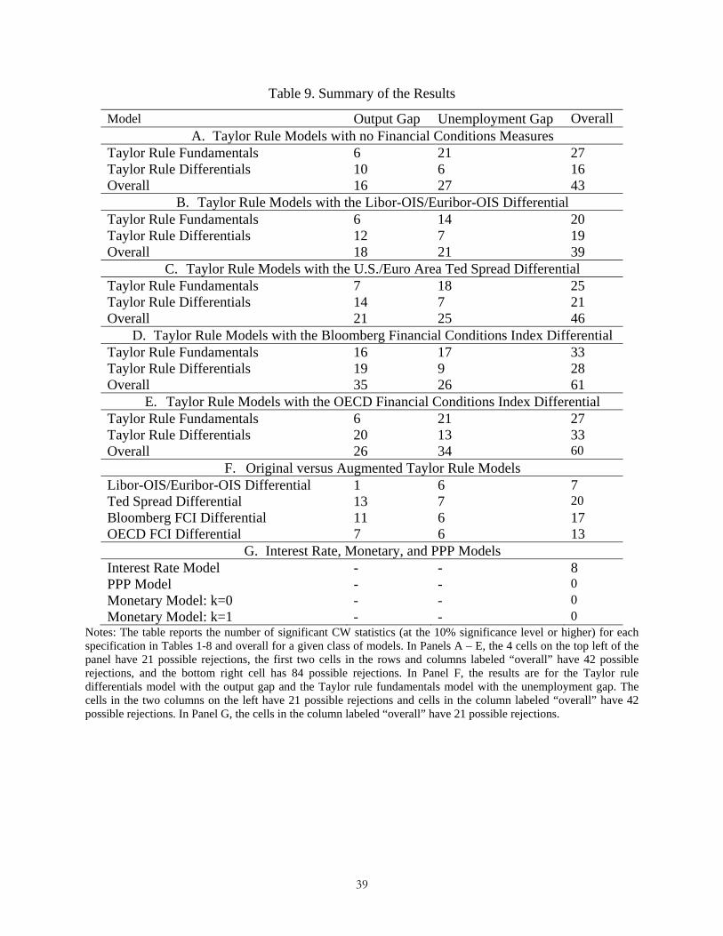
39

Table 9. Summary of the Results

Model Output Gap Unemployment Gap Overall A. Taylor Rule Models with no Financial Conditions Measures

Taylor Rule Fundamentals 6 21 27 Taylor Rule Differentials 10 6 16 Overall 16 27 43

B. Taylor Rule Models with the Libor-OIS/Euribor-OIS Differential Taylor Rule Fundamentals 6 14 20 Taylor Rule Differentials 12 7 19 Overall 18 21 39

C. Taylor Rule Models with the U.S./Euro Area Ted Spread Differential Taylor Rule Fundamentals 7 18 25 Taylor Rule Differentials 14 7 21 Overall 21 25 46

D. Taylor Rule Models with the Bloomberg Financial Conditions Index Differential Taylor Rule Fundamentals 16 17 33 Taylor Rule Differentials 19 9 28 Overall 35 26 61

E. Taylor Rule Models with the OECD Financial Conditions Index Differential Taylor Rule Fundamentals 6 21 27 Taylor Rule Differentials 20 13 33 Overall 26 34 60

F. Original versus Augmented Taylor Rule Models Libor-OIS/Euribor-OIS Differential 1 6 7 Ted Spread Differential 13 7 20Bloomberg FCI Differential 11 6 17 OECD FCI Differential 7 6 13

G. Interest Rate, Monetary, and PPP Models Interest Rate Model - - 8 PPP Model - - 0 Monetary Model: k=0 - - 0 Monetary Model: k=1 - - 0

Notes: The table reports the number of significant CW statistics (at the 10% significance level or higher) for each specification in Tables 1-8 and overall for a given class of models. In Panels A – E, the 4 cells on the top left of the panel have 21 possible rejections, the first two cells in the rows and columns labeled “overall” have 42 possible rejections, and the bottom right cell has 84 possible rejections. In Panel F, the results are for the Taylor rule differentials model with the output gap and the Taylor rule fundamentals model with the unemployment gap. The cells in the two columns on the left have 21 possible rejections and cells in the column labeled “overall” have 42 possible rejections. In Panel G, the cells in the column labeled “overall” have 21 possible rejections.