Taxonomy in Biology and Visualization

Eamonn Maguire

Oxford University Department of Computer Science

Abstract—Taxonomies are core to our everyday working. We constantly categorize entities to aid our understanding and navigationof the world around us. In the most basic of cases, we may categorize animals into dangerous or non-dangerous, pets or pestsand people into friends and strangers. Since time began, our ancestors have used taxonomy to stay away from things carrying thepotential to cause harm, and it is shown that we have the ability to classify complex entities even as children through evolved parts ofthe human brain. This paper explores the origin of taxonomy and how it carries immense importance in our world, its importance inbiology and how it is used in visualization also.

Index Terms—Taxonomy, History, Biology, Visualization.

1 WHAT IS TAXONOMY?

Taxonomy: from Ancient Greek, taxis ”arrange-ment” and nomia ”method” [20]

A general definition for taxonomy from Simpson [31] is:

”A field of science (and major component of system-atics) that encompasses description, identification, nomen-clature (naming), and classification.”

There has always been a need to identify, name and classify theentities around us. Through identifying and naming animals, insects,arachnids, plants, shapes or objects, we can adequately communicatewith others about the environment around us. The classification ofthe entities found within our environment, arranged in a hierarchicalformat are referred to as taxonomies. Taxonomies construct our viewof the world and our interactions within it. We constantly identifythings around us, even though we may not know the scientific namefor them. We also classify these things: things with fur, hair, nice shoesor nice clothes. We stay close to things which are positively reinforcedand avoid things with negative connotations [35]. For instance, eventhough one doesn’t personally know every homeless person in Oxford,most people can very quickly spot a homeless person given generalcharacteristics such a clothing, behaviour or facial complexion. Thisview we concoct is known as the umwelt, the German word for ”envi-ronment” or ”the world around” [37, 35, 22]. Within each of our ownumwelten (plural) we have different views, and often different waysof classifying things (although a lot of things will be classified in thesame way).

Over the years man has tried to name and classify the environmentaround using differing approaches. Of particular interest was classifi-cation of the organisms living around us and this is where taxonomy,in the documented sense, has its origins. Through naming and clas-sifying the organisms around us we could more clearly communicatewhich things were dangerous and which were not. We could also seewhich organisms were the same type, which things all had fur, fourlegs, two eyes and so forth. In this chapter we describe the manyapproaches taken to devise such a taxonomy by luminaries such asAristotle and Carl Linnaeus, often referred to as the fathers of sci-ence and taxonomy respectively. We also assess the use of taxonomieswithin biology, not just for classifying organisms but for classification

• Eamonn Maguire is with Oxford University, E-mail:

eamonn.maguire@st-annes.ox.ac.uk.

Manuscript received 31 March 2011; accepted 1 August 2011; posted online

23 October 2011; mailed on 14 October 2011.

For information on obtaining reprints of this article, please send

email to: tvcg@computer.org.

of chemicals too for instance. Additionally, we assess the role of tax-onomy in the field of visualization where it is playing an increasinglyimportant role in classifying types of visualizations to make it easierfor researchers and users alike to search through the cornucopia of re-sources currently available but not easily accessible.

2 TAXONOMY IN BIOLOGY

”Whats the use of their having names,” the Gnat said,”if they won’t answer to them?”

”No use to them,” said Alice; ”but it’s useful to the peo-ple that name them, I suppose. If not, why do they havenames at all?”

”I can’t say,” the Gnat replied.

- Lewis Carroll

Through the Looking-Glass

2.1 The history of taxonomies. It all started with biology

Since the origins of taxonomy lie within the field of biology, it isworthwhile to look at the history of how taxonomy evolved within thisfield and its major contributors. The timeline for the history of biologi-cal taxonomies can be split into three key periods revolving around theman regarded to be the ”father of taxonomy”, Swedish botanist CarlLinnaeus (1707-1778). These periods are pre-Linnean, Linnean andpost-Linnean.

2.1.1 Pre-Linnean (3000BC - 1707)

The concept of taxonomy did not originate with the Roman and Greekcultures as is thought by the majority of people. In fact the earliesttraces of taxonomy are from the Eastern world rather than the West[23].

Shen Nung, Emperor of China (3000 BC)The earliest form of document resembling a taxonomy dates back to3000 BC in a pharmacopeoia named Divine Husbandman’s MateriaMedica written by Shen Nung, Emperor of China. It consisted of365 plant, mineral and animal derived medicines[23]. Further tothis, in Egypt around 1500 BC medicinal plants were illustrated inwall paintings [23]. Additionally, one of the oldest papyrus rolls,named Ebers Papyrus, classified plants by their ability to treat variousdiseases of that age[23].

Aristotle (384 BC - 322 BC)Between 384 BC and 79 AD, the Greeks and Romans began totake an interest in taxonomy. Aristotle, commonly known as the”father of science”[23] was the first in the Western society to classifyall living things in Historia Animalium. His classification schemewas hierarchical and grouped organisms according to whether ornot they had similar physiological, behavioural and morphological

characteristcs, for instance animals with and without blood, animalswho live on water and those living on land. His classification systemhad no concept of evolution and the species within the hierarchieshad no known genetic relationship since this wasn’t known, theyjust looked/behaved in a similar way. Aristotle also introduced twoimportant concepts of modern taxonomy, those being: binomial (2name) definition (e.g. genus species names such as Homo sapienslater devised by Linnaeus); and classifying organisms by type[23].

Theophrastus (370 BC - 285 BC)Aristotle was succeeded by his student Theophrastus who extendedhis tutors work through the classification of all 480 known plantsin De Historia Plantarum. He subsequently became known asthe ”father of botany”. His classification scheme was based uponcharacteristics such as growth habit and fruit/seed form, introducingcategories such as trees, shrubs and herbs [23]. Many of the generanames Theophrastus developed were accepted by Carl Linnaeus [23].

Plinius (23-79 AD)After Theophrastus, 318 years passed before Plinius arrived whowrote Naturalis Historia. His main contribution to taxonomy wasthe introduction of Latin names, a contribution for which he becameknown as the father of botanical Latin [23].

Dioscorides (40-90 AD)Shortly after the arrival of Plinius, there was Dioscorides whogathered information about medicinal plants and wrote De MateriaMedica, a publication containing approximately 600 species classifiedby their medicinal properties[23].

Caesalpino (1519-1603)Until the development of optic lenses towards the end of the 16thcentury [23], the works of the Greek and Romans remained intactand there was little in the way of further classification mechanismsdeveloped. Microscopy enabled discovery of a greater number ofspecies as the level of granularity at which scientists looked at thespecimens became more and more refined. Higher granularity meantthat simply classifying things based on characteristics such as petalcolour, leaf type and so forth was no longer enough. Microscopesallowed scientists to investigate many more intricate characteristics oforganisms which led to an immediate increase in species count, sincesome things once thought to be the same were now different basedon these newly visible characteristics. The first of this new breedof taxonomists aided by this new technology was an Italian namedCaesalpino whose work named De Plantis contained 1500 species,considerably more than Theophrastus[23].

Bauhin brothers (1541-1631; 1560-1624)The Bauhin brothers, from Switzerland wrote Pinax Theatri Botanici,a revolutionary volume containing 6000 species as well as their syn-onyms, a novel feature required to bring together alternate namingsof the same species (e.g. Homo Sapiens and Human in today’s dayand age) [23]. Moreover, through grouping species by their genusand species, the Bauhin brothers were the first to use the binomialnomenclature first introduced by Aristotle.

John Ray (1627-1705)The Bauhin brothers were followed by John Ray who in 1682published Methodus Plantarum Nova containing around 18,000 plantspecies classified taking into consideration many more characteristicsof the organisms. He made great strides in his pioneering workconcerning entomological taxonomy[23].

Joseph Pitton de Tournefort (1657-1708)The final taxonomist to come along before Carl Linnaeus wasFrenchman Joseph Pitton de Tournefort) who in 1700 publishedInstitutiones Rei Herbariae containing a taxonomy of 9000 specieslisted in 698 genera classified by their floral characteristics (mostof which were accepted by Linnaeus and still in use today) [23].

It became the reference taxonomy for that botanists up until CarlLinnaeus’ publication named Systema Naturae in 1735.

2.1.2 Linnean (1707 - 1778)

Carl Linnaeus was a Swedish physician who placed botany as afocal part of his study. When Linnaeus was born in 1707, there wasno shortage of botanical classification systems in use. However,there was no one size fits all naming convention or classificationmethod developed and the result was no consistency where thesame plants had numerous names. The Bauhin brothers applied apragmatic yet short term approach to resolve this problem through theintroduction of synonyms to species descriptions, but as new specieswere continually being discovered as world exploration reached anew level, the situation was quickly becoming unmanageable. In anattempt to quell the potential name epidemic, Linnaeus publishedCritica botanica in 1735 which presented guidelines to be followedfor creation of generic names, extending Aristotle’s introduction ofbinomial definition into the naming scheme of the world’s flora andfauna [23]. This two part name was constructed from the genus(always capitalized) and the species name (always lower case), e.gHomo sapiens. Further to this, Linnaeus realized the need to notonly harmonize the names of species, but to also control the waythey are described. Linnaeus introduced rules for how to constructspecies description and the terminology to use in two publications,Fundamenta botanica in 1736 and Philosophia botanica in 1751 [23].

KINGDOM Animalia

PHYLUM Chordata

CLASS Mammalia

ORDER Primates

PHYLUM Hominidae

GENUS Homo

SPECIES sapiens

Fig. 1. Linnaean Classification of Homo sapiens.

In developing a common classification method, Linneus wrotehis most important work Systema Naturae or The System of Nature.Published in 1735, it provided an overall classification frameworkfor all plants and animals from kingdom to species level (Kingdom -Phylum - Class - Order - Phylum - Genus - Species see figure 1 foran example classification) [33, 23]. Over the course of 10 editions,the last of which was published in 1758 and whose full title wasSystema naturae, sive regna tria naturae systematice proposita perclasses, ordines, genera, and species, Linnaeus fixed errors such asthe positioning of whales as fish and he was the first to put humansamongst primates and classify us using the binomen Homo sapiens.Further to Systema Naturae, Linnaeus’ plant classification, influencedby Cesalpino, was described in two publications named The Genera ofPlants and The Species of Plants. His classification method built uponTournefort’s method of classification, however Linnaeus extended thismethod considering that plant’s had a sexuality based on the presenceof stamens and pistils [23].

In his quest for perfection, Linnaeus became the ”father of taxon-omy”. His constant refinement of his methodology based on emerg-ing species and developments in science enabled the pervasive use ofhis classification methods. Moreover, his foresight in being able tonot only solve many of the problems of that time in creating commonclassifications, but also to introduce standard naming conventions andspecies descriptions was critical in making the science of taxonomywhat it is today.

2.1.3 Post-Linnean

Many of the taxonomies we use today are still based on Linnaeus’work back in the 18th Century. However, back in those times, noteveryone agreed with Linnaeus’ classification approach, the Frenchin particular. Disagreements were in general justified. Linnaeus’sclassification approach was very subjective and categorised thingsbased on observed phenomena, such as whether or not an animal hadfur, hair, 4 legs and so forth. Four French scientists, from 1707 -1829 including George-Luise Leclerc de Buffon (1707-1788), MichelAdanson (1727-1806), Antoine Laurent de Jussieu (1748-1836)and Jean-Baptiste de Lamarck (1744-1829) challenged the ideasof Linnaeus and bettered the taxonomic field as a whole throughcontributions including new theories about evolutionary traits forexample.

George-Luise Leclerc de Buffon (1707-1788)George-Luise Leclerc de Buffon’s criticisms were based on the factthat Linnaeus was imposing order on a chaotic natural world. Hedeveloped theories about how species develop, varieties within speciesand inherited characteristics in species [23]. This work provided theplatform on which evolutionary biology was based.

Antoine Laurent de Jussieu (1748-1836)Antoine Laurent de Jussieu bettered Linaeus’ classification of plantswith Genera Plantarum in 1789. He launched a natural classifica-tion system based on many plant characteristics which are now usedin modern classification systems [23]. He introduced the classifica-tions of acotyledons, monocotyledons and dicotyledons and added the”family” rank in between”genus” and ”class” [23].

Jean-Baptiste de Lamarck (1744-1829)Jean-Baptiste de Lamarck developed an evolutionary theory whichalso included the inheritance of characteristics between species [23].

Darwin era (1809-1882) and evolutionary theoryAlthough the notion of evolution was presented before CharlesDarwins time by Lamarck and de Buffon for instance, it was notfully explored until Darwin and Alfred Russel Wallace (1823-1913)launched the evolutionary theory in 1858. Following this, twoGerman biologists, Ernst Haeckel (1824-1919) and August WilhelmEichler (1839-1878) composed ideas to incorporate evolution intotaxonomies. It was Haeckel who eventually established the term”phylogeny” leading to what we now know as phylogenetic treeswhich visually group similar things together based on the pres-ence/absence of characteristics between organisms or more recentlytheir genetic distance.

Willi Hennig (1913-1976) and cladisticsGerman biologist Willi Hennig (1913-1976) founded a new classifi-cation method called cladistics (or phylogenetic nomenclature) in1966 which was intended to be a more objective method for classi-fication organisms. Cladistics stated that only similarities groupingspecies, called synapomorphies should be used in classification andtaxa should include all descendants from one single ancestor (mono-phyly). An example cladogram is shown in figure 2.

The problem with phylogenetic trees is that they typically yield ahigh number of possible trees for any given number of taxa and sub-sequent characteristics, be these genetic or phenetic: 3 taxa yield 3trees; 4 taxa yield 15 trees; 7 taxa yield 10,000 trees; and with 10taxa, there is a possible 34 million trees [32]. In an attempt to resolvethis, cladistics introduced parsimony, where the best phylogenetic treeis one which requires the least number of evolutionary changes. Anexample is worked through in figure 3.

The value of cladistics wasn’t realised by everyone when it wasinitially proposed. When Willi Hennig suggested clasdistics as an ap-proach, scientists were more interested in phenetics, which dominatedfor years after. Phenetics involved grouping organisms by many dif-ferent characteristics and was perceived to be much more subjectivethan classic Linnaean classifications. It wasn’t until when PCR (poly-merase chain reaction) and DNA sequencing started to come on the

Animals

Slime moulds

Plants

Algae

Protozoa

Crenarchaeota

Nanoarchaeota

Euryarchaeota

Protoeobacteria

Acidobacteria

Thermophilic

sulfate-reducers

Cyanobacteria

(blue-green algae)

Fusobacteria

Spirochaetes

Planctomycetes

Actinobacteria

Green nonsulfur bacteria

Chlamydiae

Gram-positivesFungi

Fig. 2. Tree of life as a cladogram. Source: Wikipediahttp://en.wikipedia.org/wiki/File:CollapsedtreeLabels-simplified.svg

scene in the 70s, that the cladist approach started to make more senseand picked up momentum. Additionally, calculating 34 million possi-ble trees using computers in the 70’s wasn’t very feasible unless onehad access to large university supercomputers, and this is only a smallexample with 10 taxa! Building up a complete tree of life or evenclade takes a huge amount of computation which until relatively hasnot been possible.

Moving toward cladistics & PhyloCode (1970s - present)As a result of this proliferation of sequences and subsequent computa-tional analysis, we’ll find that lots of organisms don’t belong in theirLinnaean classification any longer. With Linnaean classifications, newdiscoveries can require renaming of classes, orders or kingdoms (orcombinations of all three). Over the last 30 years, there has beencontinuing refactoring of the classification tree to make the branchesmonophyletic (one common ancestor). This will continue to happenas we continue to receive more sequence data. Conversely, the cladistapproach was developed with the assumption that the shape of the treecan change, making it inherently less difficult to add/remove/changeclassifications as time goes on.

Even though cladistics is in use today, it is again not without it’scritics. For instance, when comparing species based on genetic traitsand genetic distance where our matrix for parsimony is now basedon the probability that adenine can change to thymine, guanine canchange to cytosine and vice versa, we fail to take into considerationwell know concepts such as lateral gene transfer or events such asthose where bacteria cells can have viral DNA. As a result (as un-likely it might be), our classification can be wrong and possibly placea bacteria in the same clade as a virus, simply because they share alarge proportion of the same DNA. There is also a criticism in the useof parsimony. The assumption that the best tree is the one with thefewest number of evolutionary steps is not necessarily true since evo-lution doesn’t always do things in a straightforward manner.

Even so, there are still movements towards cladistics and away fromLinnaean nomenclature and classification. Borne within these move-ments, the PhyloCode project [3] started in 1998. The concept of Phy-loCode is that species and clades should have names, but all ranksabove species are excluded from the nomenclature [3, 23]. The projectis regarded as controversial within the bio taxonomic community, butrepresents the latest suggested change in how classifications could becreated.

2.2 Other taxonomies within biology

Taxonomies or ontologies (which are more formal than basic tax-onomies with rules, restrictions, etc.) are used in many parts of bi-ology in order to structure domain knowledge in order to aid scientistsin consistently identifying chemicals or genes for instance:

• biochemistry: naming and describing chemicals and smallmolecules, and classifying these (see figure 4). See the chem-ical entities of biological interest ontology ChEBI [1]; and

Apatosaurus

Brachiosaurus

Characteristic number

Camarasaurus

Common Anc.

from 3 taxa we can construct 3 possible trees. These are:

we have a matrix of the taxa we which to classify and whether or

not they have the characteristics defined above

Apatosaurus

Brachiosaurus Camarasaurus Apatosaurus

Brachiosaurus

Camarasaurus

Apatosaurus Brachiosaurus

Camarasaurus

Characteristics

1. Cervical ribs extend past at least one whole vertebra

2. Bifurcated neural spine in cervical vertebrae

3. Tibia as broad at distal as at proximal end

4. Chisel-like teeth (not peg-like)

we then calculate the length of the trees proposed, this is the number of

evolutionary changes required to construct the tree from the matrix

above

common ancestor is a dummy entry used to calculate the

parsimony of the final tree created.

e.g. calculating for tree 1

Apatosaurus

Brachiosaurus Camarasaurus

Common anc.

char 1 requires one change

Apatosaurus

Brachiosaurus Camarasaurus

Common anc.

char 2 requires two changes

1

1

1

Apatosaurus

Brachiosaurus Camarasaurus

Common anc.

char 3 requires one changes

1Apatosaurus

Brachiosaurus Camarasaurus

Common anc.

char 4 requires one changes

1

in total, tree 1 fits in 5 changes/transitions. Length = 5.

Applying the same method to trees 2 and 3, we find that tree 2

requires 6 transitions and tree 3 requires 7.

Therefore, tree 1 is the best fit.

Apatosaurus

Brachiosaurus Camarasaurus

Fig. 3. Characteristic matrix is constructed given 3 taxa. 3 taxa yields3 possible trees and the best tree is selected based on the one that re-quires the fewest number of changes to be constructed. Diagram con-structed based on content from Taylor [32].

Fig. 4. High level classifications in the ChEBI ontology [17, 1], as viewedin BioPortal

• genes: describing the biological processes, cell location andmolecular functions of genes. See the gene ontology in BioPortalGO [15, 2].

Consistently describing organisms, chemicals, genes, biologicalprocesses and so forth is very important in allowing for accurate dis-semination of knowledge.

2.3 Summary of biological taxonomies

Every taxonomy created will come under scrutiny as a result of thenature of the task at hand. We are asking scientists to map continu-ous phenomena in terms of evolution and speciation to discrete spacewhich is inevitably going to be challenging and always artificial [21].Moreover, as more and more DNA sequencing continues to happen,there will be many shifts in the tree of life as there was when micro-scopes first became available back in the 16th century.

Even though criticisms of taxonomies (and ontologies) exist and areoften far from complete or accurate, they are also hugely importantin our understanding of biodiversity and the world around us. For in-stance, in human metagenome studies, we can identify microbes livingin and on our bodies and the effects of such populations on health[9].In microbial ecology, we can discover the species prevalent in partic-ular habitats, for example, which bacteria are present in areas wherean oil spill has occurred [19]. Having well defined taxonomies and in-formation about the species, studies like those described can happen.Without such taxonomies, we would have no idea what exists in theenvironment around us.

Extending on this point, as we continue to sequence and study moreand more of our ecology and personal microbiomes via initiatives suchas the human and earth microbiome projects [26], challenges are be-ing encountered when defining when exactly a new species has beenfound. There is still a lot of uncertainty over how to define a newspecies and how much natural in-species variation is allowed [21, 24].There needs to be more work carried out to make systematic decisionsabout what is a new species and what is not. From 1993 - 2005, thenumber of mammalian species alone has grown from 4,659 to 5,418[25]. Given that the microbial populations are magnitudes in size big-ger, we are set for a taxonomic explosion unless a more systematicapproach is put in place.

3 TAXONOMIES IN VISUALIZATION

The idea of a visualization taxonomy first appeared in 1992 and wasintroduced by Brodlie from the University of Leeds [8]. Since thenthere have been numerous taxonomies developed to try and capturewhat happens within the visualization field. We typically wish to cat-egorize the following areas of visualization:

• 1. the type of visualization, e.g. the data being represented andthe way we’ve represented it;

• 2. how we created the visualization (processes), so the assump-tions that were made when abstracting the information from theinitial data source and when creating the visual mappings; and

• 3. the organisation of visual taxonomies and subsequent visualmetaphors to represent real world concepts (semiotics).

1 and 2 are very much related and are mechanisms for categorisingvisualization techniques in general. 3 on the other hand diverges fromthe normal idea of classifying things within visualization such as dataor chart types and instead focuses on how one may leverage off ofthe internal taxonomies we carry with us to create icons/signs/glyphswhich map to real life phenomena, e.g. a cross on a map correspondsto a church or a red H maps to a hospital.

The end result is that a visualization taxonomy should be able to:

• help users in navigating the huge visualization tool space. Byadequately categorising visualizations users could more easilyfind the visualization that is right for them; and

• help researchers in finding out about similar work in their fieldor work that can add value to their research.

3.1 Taxonomies for visualization techniques

Two ways currently explored for the creation of visualization tax-onomies are to:

• classify by the type of the data being visualized, e.g. discreteor continuous data. This is the most common way to classifyvisualizations; and

• classify by the processes/algorithms used to process and renderthe data, a relatively new method of classification.

3.1.1 Focusing on visualization data type

Most of the taxonomies created in the past have focused on data type.The categories defined have historically made the split on discretevs continuous or scientific vs non-scientific data, indicated by factorssuch as; application area; whether the data is physically based (scien-tific visualization) or abstract (information visualization); and if spatialinformation is given (scientific visualization) or not (information visu-alization) [34]. The problem with such a taxonomic hierarchy is thatthere are many examples which cross both classifications, so classify-ing something simply because it has to go somewhere would be inher-ently wrong. Below we document some of the major developments invisualization taxomonies and look at how they are structured.

In 1996, Shneiderman described a taxonomy for visualizationwhich was data centric but also included a taxonomy on how to nav-igate through the visualization space based on a ”visual informationseeking mantra” of ”overview first, zoom and filter, then details ondemand”[29]. The taxonomy is arranged as follows [29]:

• Data types:

– 1-dimensional e.g. textual documents & program sourcecode;

– 2-dimensional e.g. geographic maps & floor plans;

– 3-dimension e.g. molecules & the human body;

– multi-dimensional e.g. items with n attributes which be-come points in a n-dimensional space;

– temporal e.g. project management & historical representa-tions of data;

– tree e.g. file hierarchies;

– network e.g. protein-protein interaction networks & socialnetworks;

• Interactions,:

– Overview;

– Zoom;

– Filter;

– Details-on-demand;

– Relate;

– History;

– Extract;

The visualization taxonomy from Shneiderman has been appliedby his students to create an online resource called the On-lineLibrary of Information Visualization Environments (OLIVE) [4] whichcategorizes projects, products and publications by the data typesdefined in the taxonomy.

In 1997, Card and Mackinlay devised another data-oriented taxon-omy [11] which was then expanded on in 1999 in a collaboration withShneiderman [10]. The overall contribution of this work was to splitvisualization into a number of categories. These were:

• Scientific Visualization;

• GIS;

• Multi-dimensional Plots;

• Multi-dimensional Tables;

• Information Landscapes and Spaces;

• Node and Link;

• Trees;

• Text transforms;

In 1998, Ed Chi proposed a taxonomy focusing on not only thedata, but also the processes these data goes through to create a visu-alization [14]. This taxonomy is called the Information VisualizationData State Reference Model (or Data State Model). A graphical depic-tion of the taxonomy is shown in figure 5. The concept is to classifyvisualizations on the type of data they work on (temporal, network,multi-dimension etc) and the transformations such data goes throughto create the final visualization including data abstraction, visual ab-straction and visual mappings.

The generic nature of Chi’s taxonomy makes it able to classifymany visualization techniques and numerous examples are docu-mented in Chi’s follow up publication in 2000[13]. The concepts de-scribed in Chi’s paper have also been applied in creating more domainspecific taxonomies as exemplified by Daasi et al [16].

Furthermore, have been additional visualization taxonomies sug-gested in some non-scientific publications which categorise visualiza-tions by the type of operation they support For instance, Dan Roampresented the Visual Thinking Codex (see figure 6) in his book namedThe Back of the Napkin [27].

In this figure Roam organises visualization types by what they aretrying to divulge to the reader of the visualization: who/what, howmuch, where, when, how and why? Additionally, there are subcate-gories on if the visualization is simple vs elaborate in terms of detailor qualitative vs quantitave for example.

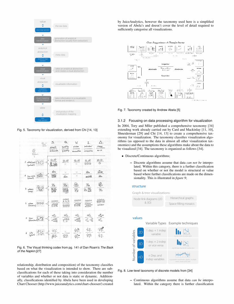
Andrew Abela [5] also presented a technique for taxonomising vi-sualizations. This is shown in figure 7. The high level (comparison,

value

value stage operator

analytical

abstraction

analytical stage operator

data transformation

visual

abstraction

visualizationstage operator

visual transformation

view

viewstage operator

visual mapping transformation

the raw data

meta-data

visualizable information

end-product of the visualization mapping

takes an analytical abstraction and creates a visual abstraction

takes information in a visualizable format and renders it.

generation of analytical abstraction (usually from extraction)

Fig. 5. Taxonomy for visualization, derived from Chi [14, 13]

Fig. 6. The Visual thinking codex from pg. 141 of Dan Roam’s The Backof the Napkin.[27]

relationship, distribution and composition) of the taxonomy classifiesbased on what the visualization is intended to show. There are sub-classifications for each of these taking into consideration the numberof variables and whether or not data is static or dynamic. Addition-ally, classifications identified by Abela have been used in developingChart Chooser (http://www.juiceanalytics.com/chart-chooser/) created

by JuiceAnalytics, however the taxonomy used here is a simplifiedversion of Abela’s and doesn’t cover the level of detail required tosufficiently categorise all visualizations.

Fig. 7. Taxonomy created by Andrew Abela [5]

3.1.2 Focusing on data processing algorithm for visualization

In 2004, Tory and Mller published a comprehensive taxonomy [34]extending work already carried out by Card and Mackinlay [11, 10],Shneiderman [29] and Chi [14, 13] to create a comprehensive tax-onomy for visualization. The taxonomy classifies visualization algo-rithms (as opposed to the data in almost all other visualization tax-onomies) and the assumptions these algorithms make about the data tobe visualized [34]. The taxonomy is organized as follows [34].

• Discrete/Continuous algorithms;

– Discrete algorithms assume that data can not be interpo-lated. Within this category, there is a further classificationbased on whether or not the model is structural or valuebased where further classifications are made on the dimen-sionality. This is illustrated in figure 9;

structure

values

Graph & tree visualizations:

Node-link diagrams (2D

& 3D)

Hierarchical graphs

Space-filling mosaics

1 dep. + 1 indep

variable

1 dep. + 2 indep

or vice versa

n Dep. and

indep variables

e.g bar chart & scatter plot

e.g 3D bar chart & 3D scatter plot

e.g parallel coordinates, glyphs, multiple

views, charts and color

Fig. 8. Low-level taxonomy of discrete models from [34]

– Continuous algorithms assume that data can be interpo-lated. Within the category there is further classification

based on the data structure (scalar, vector, tensor or multi-variate and the number of independent variables.);

multiple 1D, 2D, or 3D views

scalar vector tensor multi-variate

combine scalar,

vector & tensor

methods

line graph

colour map

isolines

volume

rendering

isosurfaces

LIC

particle

traces

glyphstensor

ellipsoids

Fig. 9. Low-level taxonomy of continuous models from [34]

• Display Constraints. Discrete and continuous algorithms are fur-ther classified by whether or not the display constraints are given,constrained or chosen.;

– Given, e.g. air traffic positions (discrete), or images (con-tinuous);

– Constrained e.g. arrangement of ordinal/numeric values(discrete), or 2D geographic maps (continuous);

– Chosen e.g. file structures (discrete) or regression (contin-uous);

• Visualization Tasks. For each type of visualization, there willbe different types of tasks that can be performed, something thatwasn’t detailed in the taxonomy created by Shneiderman [29](see figure 10);

– When spatialization is given: user should be able to spec-ify regions of interest, extract information and/or examineinformation in greater detail;

– Discrete structural models allow pattern analysis: user canidentify outliers and clusters of data points as well as filterdata;

– Continuous models (and discrete value models holding or-dinal data) allow users to see numerical trends;

There is much novelty in the algorithm compared with other tech-niques focusing on just the data type. However, in my opinion thereis still fuzziness in how the classification is made at the top level asdemonstrated in table 1 of the paper [34] where display attributes con-strained on spatialization yield duplicated examples in two separateclassifications.

3.2 Taxonomies and semiotics

All seeing humans, animals, insects and so forth have a visual tax-onomy, things are seen and meaning is constructed from previous in-ferred or known knowledge. For instance, we see a red sign on a roadand immediately take notice since we know that red generally means’warning’. Similarly, if we see an insect with bright colours (red inparticular), it is natures way of telling us to watch out, that insect ismost probably poisonous (or pretending to be). Interestingly, noonehas taught us that red means danger, it is known. Red is in our inter-nal taxonomy, there since we were born to tell us that red things areusually dangerous. The relations between the visual and their mean-ing has been investigated many times over by authors such as JakobVon Uexkll [35], Jacques Bertin [7, 6] and Umberto Eco [18] in a fieldnamed semiotics.

Patterns (e.g. clusters, outliers)

Connectivity relationships

Spatial relationships

Spatial regions of

interestNumeric trends

Item details, Filtering (item exclusion)

Fig. 10. Classification of visualization tasks. Tasks are defined basedon whether the spatialization is given or chosen and if the design modelis continuous or discrete. Adapted from [34]

Semiotics, or the study of signs and sign processes (semiosis) [36].Semiotics as a field also encompasses how meaning is constructed andunderstood [36]. It is typically split up into 3 branches[36]:

• semantics: relation between signs and what they refer to (deno-tata);

• syntactics: relation among signs; and

• pragmatics: relation between signs and the effects they have onthe people who use them.

Although semiotics is not confined solely to the visual system (itcan also apply to meaning we give to scent)The application of semi-otics in the context of visualization is particularly important when us-ing visual metaphors to represent something. For instance, in cartog-raphy a cross has a meaning which happens to be a church (see figure10. However, in a biological experiment workflow visualization, across may mean that an animal died. Within each field, the symbolmeans something different. Similary, a line on a map could indicate aroad, however in the context of a biological experiment, a line can of-ten be used to represent a DNA strand (see figure 11. These examplesrefer to the semantics of the sign.

In addition to this, we could use combinations of signs to createmore complex structures with more meaning (e.g. this sentence), thisrefers to the syntactics. We could also organise these signs into tax-onomies (where we have a hierarchy) to create a visual taxonomy, asmall example of which is in figure 12 where we arrange glyphs (vi-sual entities representing information) in a hierarchical format basedon classifications on data and material centric processes.

We can also use taxonomies to classify the properties of glyphs likethose shown in figure 12. For instance, we may want to classify glyphsby the pre-attentive (things we take in about entities with paying muchattention) and attentive (things we have to pay more attention to inorder to take in its message) stimuli utilized in their creation. This hastwo major advantages:

• 1. it highlights the importance in considering such propertieswhen creating glyphs; and

• 2. it would make it possible to search for glyphs based on theircharacteristics, e.g. shape, colour, etc.

Such a taxonomy has been created by Ropinski and Preim [28].This taxonomy is summarised in figure 13.

Fig. 11. The meaning of abstract images in differing fields, their se-mantics. a) a cross on a map has a meaning ’church’. b) a line in abiology themed visualization has the meaning ’DNA’. Use of these ab-stract structures to represent complex ones is key to cartography andglyph based visualizations in particular.

process

data processmaterial process

filtrationhybridization cell lysis regression pca

Fig. 12. Small example of a taxonomy for bio experiment processes util-ising glyphs to represent information. We have an upper level processwhich has a certain shape and colour and have additional details insideas we go lower in the taxonomy. The process category has a constantouter shape.

pre-attentive

attentive

parameter mapping

placement

parameter mapping

graphic legend

interactiverepositioning

change mapping

discrete

continuous

single

multiple

composite shape

directional

non-directional

data set driven

feature driven

discrete

continuous

jittering

packing

basic shape

blurring

color

colortransparencytexture

Fig. 13. Glyph taxonomy as presented in Ropinski and Preim [28].

3.3 Summary

The field of visualization taxonomy is much newer than say that ofthe biological domain but the benefits of having a taxonomy are to be-come clearly apparent when trying to navigate the growing visualiza-tion space. Some elements not covered by current taxonomies thoughis the definition of data, information and knowledge as discussed by

Chen et al [12]. This is particularly important since the majority oftaxonomies discussed in this section are providing classifications ondata, the definition of which is interchangeable between fields. Futuretaxonomies should attempt to provide a definition of these terms.

There has been good progress in the development of a visualizationtaxonomy, and this will improve more given the development of visu-alization ontologies like that presented in Shu et al 2006 [30] and thecontinued rise of the semantic web and the linked data vision. It willtherefore be important to ensure that descriptions of visualization toolsare exposed in a semantically meaningful way. Moreover, being ableto describe how visualizations were created (in the processes invoked)would allow for reproducibility of visualization tasks or could informusers better about the data rendered for them. For example, it is typicalfor visualizations to be presented to users but masking out uncertaintyin terms of statistical bias, error ranges and so forth. Through inform-ing users in a standardised way about how a visualization came to beconstructed, they can make more informed decisions about whether aparticular result is good or not, or can search through visualizationscreated using particular statistical methods for instance.

4 CONCLUSION

Although taxonomies originated in the field of biology, their applica-tion is pervasive and they are used to categorize content on a broadscale. However, taxonomies are unlikely to ever be perfect for a num-ber of reasons:

• 1. we are mapping continuous phenomena into discrete space. Itis an unnatural mapping and will almost certainly not be perfect;

• 2. there are always exceptions to the norm; and

• 3. there is an inability to unanimously agree with consensus.

Yoon approached this subject of imperfection in the book NamingNature: The Clash Between Instinct and Science[37] in which shealso refers to the umwelt concept when it comes to constructingtaxonomies. In this book she states that since we have an inbuiltsystem of classification for the world around us as humans, classify-ing everything, that within our environment scope and without willinevitably lead to unnatural and incomplete classifications. As anextreme example, when thinking about the olfactory (smell) system,humans are much less sensitive to smell than dogs[37]. Thereforethe way dogs classify things in their environment will be inherentlydifferent to the classification of the same environment by humans. Ifwe apply this to people from differing cultures or generations, we willnot get the same extreme variance we would get with a dog, but therewill be some differences in the classifications that we get of the samething. This is inherently problematic when it comes to those whomake the decisions about what makes a species and what doesn’t orwhich classification is best for visualization taxonomies.

That being said however, modelling our world as close as possibleto the real world and in a generic a way as possible will certainly beuseful in guiding users and researchers in describing and navigatingdomains (biology, chemistry) in a consistent way, something of grow-ing importance in anticipation of the semantic web.

REFERENCES

[1] Chemical entities of biological interest.

http://bioportal.bioontology.org/ontologies/46576/.

[2] Gene ontology. http://bioportal.bioontology.org/ontologies/1070/.

[3] Phylocode. http://www.ohiou.edu/phylocode.

[4] Olive. http://otal.umd.edu/Olive/, 1999.

[5] A. Abela. Visualization taxonomies.

http://extremepresentation.typepad.com/blog/2008/06/visualization-

taxonomies.html.

[6] J. Bertin. Semiology of graphics:diagrams, networks, maps. 1983.

[7] J. Bertin and M. Barbut. Semiologies graphique. Mouton, Paris, 1973.

[8] K. Brodlie. Scientific visualization: techniques and applications.

Springer-Verlag, 1992.

[9] J. Caporaso, C. Lauber, E. Costello, D. Berg-Lyons, A. Gonzalez,

J. Stombaugh, D. Knights, P. Gajer, J. Ravel, N. Fierer, J. Gordon, and

R. Knight. Moving pictures of the human microbiome. Genome Biology,

12(5), 2011.

[10] S. Card, J. Mackinlay, and B. Shneiderman. Information Visualization:

Using Vision to Think. Morgan Kaufmann, San Francisco, 1999.

[11] S. Card and J. MacKinley. The structure of the information visualization

design space. Proc. IEEE Symposium on Information Visualization, 1997.

[12] M. Chen, D. Ebert, H. Hagen, R. S. Laramee, R. van Liere, L. K.-L. Ma,

W. Ribarsky, G. Scheuermann, and D. Silver. Data, information, and

knowledge in visualization. IEEE computer graphics and applications,

29(1), 2009.

[13] E. H. Chi. A taxonomy of visualization techniques using the data state

reference model. Information Visualization. InfoVis, pages 69–75, 2000.

[14] E. H. Chi and J. T. Riedl. An operator interaction framework for visual-

ization systems. Symposium on Information Visualization, pages 63–70,

1998.

[15] G. O. Consortium. The gene ontology in 2010: extensions and refine-

ments. Nucleic acids research, 38 (Database Issue):331–335, 2010.

[16] C. Daassi, L. Nigay, and M.-C. Fauvet. A taxonomy of temporal data

visualization techniques. 2006.

[17] K. Degtyarenko, P. de Matos, M. Ennis, J. Hastings, M. Zbinden, A. Mc-

Naught, R. Alcantara, M. Darsow, M. Guedj, and M. Ashburner. Chebi: a

database and ontology for chemical entities of biological interest. Nucleic

Acids Research, 2008.

[18] U. Eco. A theory of semiotics. Indiana University Press, 1979.

[19] B. Edwards, C. Reddy, R. Camilli, C. Carmichael, K. Longnecker, and

B. V. Mooy. Rapid microbial respiration of oil from the deepwater hori-

zon spill in offshore surface waters of the gulf of mexico. Environmental

Research Letters, 6(035301), 2011.

[20] D. Harper. Taxonomy.

[21] A. Helbig, A. Knox, D. Parkin, G. Sangster, and M. Collinson. Guidelines

for assigning species rank. Ibis, 144:518–525, 2002.

[22] K. Kull. Jakob von uexkuell: An introduction. Semiotica, 2001(134):1–

59, 2001.

[23] M. Manktelow. History of taxonomy. Lecture from Dept. of Systematic

Biology, Uppsala University, 2010.

[24] E. Mayr. What a species is and what is not? Phil Sci, 63:26–77, 1996.

[25] S. Meiri and G. Mace. New taxonomy and the origin of species. PLoS

Biol, 5(7), 2007.

[26] L. Proctor. The human microbiome project in 2011 and beyond. Cell host

and microbe., 10(4):287–291, 2011.

[27] D. Roam. The Back of the Napkin. 2008.

[28] T. Ropinski and B. Preim. Taxonomy and usage guidelines for glyph-

based medical visualization. Proceedings of the 19th Conference on Sim-

ulation and Visualization (SimVis08), 2008.

[29] B. Shneiderman. The eyes have it: A task by data type taxonomy for in-

formation visualization. Proceedings IEEE Workshop Visual Languages,

pages 336–343, 1996.

[30] G. Shu, N. Avis, and O. Rana. Investigating visualization ontologies. Pro-

ceedings of the UK e-Science All Hands Conference 2006., pages 249–

257, 2006.

[31] M. G. Simpson. Plant Systematics. Academic Press., 2nd edition, 2010.

[32] M. Taylor. What is cladistics? how reliable is it?

http://www.miketaylor.org.uk/dino/faq/s-class/clad/index.html, 2003.

[33] L. Tilton. From aristotle to linnaeus: the history of taxonomy.

http://davesgarden.com/guides/articles/view/2051/.

[34] M. Tory and T. Moller. Rethinking visualization: A high-level taxonomy.

IEEE Symposium on Information Visualization, pages 151–158, October

2004.

[35] J. von Uexkull. An introduction to umwelt. Semiotica, 2001:107–110,

1998.

[36] Wikipedia. Semiotics. http://en.wikipedia.org/wiki/Semiotics.

[37] C. K. Yoon. NAMING NATURE: The Clash Between Instinct and Science.

W. W. Norton and Company, 2010.