Tax evasion, financial development and inflation:

theory and empirical evidence∗

Manoel Bittencourt† Rangan Gupta‡ Lardo Stander§

February 2013

Abstract

Using a standard overlapping generations monetary production econ-omy, faced with endogenously determined tax evasion by heterogeneousagents in the economy, we provide a theoretical model that indicatesthat both a lower (higher) level of financial development and a higher(lower) level of inflation leads to a bigger (smaller) shadow economy.These findings are empirically tested within a panel econometric frame-work, using data collected for 150 countries over the period 1980−2009to enable a broad generalisation of the results. The results support thedeveloped theoretical model, even after having accounted for the differ-ences in the levels of economic development, the level of institutionalquality that includes different tax regimes and regulatory frameworks,central bank participation in the economy as well as different macroe-conomic policies.

JEL Classification: C61, E26, P16Keywords: Informal economy, financial development, inflation.

∗We would like to thank two anonymous referees for many helpful comments thattremendously improved the quality of the paper. However, any remaining errors are solelyours.†Department of Economics, University of Pretoria, Pretoria, 0002, South Africa.‡To whom correspondence should be addressed. Department of Economics, University

of Pretoria, Pretoria, 0002, South Africa, Email: rangan.gupta@up.ac.za.§Department of Economics, University of Pretoria, Pretoria, 0002, South Africa.

1

1 Introduction

”To think of shadows is a serious thing.” - Victor Hugo1

Recent empirical evidence provided by Bose, Capasso and Wurm (2012)show that an improvement in the development of the banking sector is as-sociated with a smaller shadow economy. The findings of Bose et al. (2012)corroborate indicative theoretical results reported by Blackburn, Bose andCapasso (2010) that a less-developed financial sector corresponds to the ob-servance of a bigger shadow economy. Blackburn et al. (2010) studied therelationship between the underground economy and financial developmentin a model of tax evasion and bank intermediation. In their model, agentswith heterogeneous skills seek loans in order to undertake risky investmentprojects, with asymmetric information between borrowers and lenders im-plying a menu of loan contracts that induce self-selection in a separatingequilibrium. Given these contracts, agents choose how much of their in-come to declare by trading off their incentives to offer collateral againsttheir disincentives to comply with tax obligations. The main implication ofthe analysis is that the marginal net benefit of income disclosure increaseswith the level of financial development. Thus, as with the empirical obser-vation made by Bose et al. (2012), the paper shows that the lower is thestage of such development, the higher is the incidence of tax evasion and thegreater is the size of the underground economy. Furthermore, Gupta andZiramba (2010) using an overlapping generations (OLG) monetary endoge-nous growth model, whereby government transfers affect young-age income,show that inflation - besides the usual suspects like fiscal policy (Dabla-Norris and Feltenstein, 2005), penaly rates (Schneider, 1994), probability ofbeing detected (Schneider and Enste, 2000) and degree of corruption (Cer-queti and Coppier, 2011) - affect the degree of tax evasion. Specifically, theyindicate a negative relationship between inflation and the fraction of incomereported.

Against this backdrop, the objectives of this paper are twofold: First,using a monetary OLG stochastic production economy, characterised byendogenous tax evasion, we provide a novel theoretical explanation that bothlower financial sector development as well as higher inflation (money growthrate) leads to a bigger shadow economy, and; second, with the theoreticalanalysis presented yielding an empirically-testable equation (albeit not inthe sense of a one-to-one correspondence) relating tax evasion with financialdevelopment and inflation, we test the validity of the theoretical implicationsusing a panel of 150 countries for the period 1980 to 2009, based on a newly-constructed dataset of shadow economy estimates by Elgin and Oztunali(2012).2 To the best of our knowledge, this paper is not only the first

1Les Miserables (1862).2Note that the shadow economy estimates of Elgin and Oztunali (2012) is obtained

2

attempt at providing a simultaneous theoretical explanation of how both(lower) financial development and (higher) inflation may lead to (higher)tax evasion and therefore, to the observance of a (bigger) shadow economy,3

but also empirically corroborate the theoretical claims.At this stage, it is important to put into context the importance of

our theoretical result that monetary policies (money growth rate and cash-reserve requirements held by financial intermediaries4) could also affect thelevel of tax evasion. Gupta (2008) and Gupta and Ziramba (2009) pointout that studies (such as Roubini and Sala-i-Martin (1995), Gupta (2005)and Holman and Neanidis (2006)) which analyse optimal (growth- and/orwelfare-maximising) mix of fiscal and monetary policy suffer from the Lucas(1976) critique, by treating tax evasion exogenously. Gupta (2008) andGupta and Ziramba (2009) reached such conclusions by developing growthmodels with tax evasion being a behavioural decision (as also pointed outtheoretically by Atolia (2003), Chen (2003) and Arana (2004)) to indicatethat the level of tax evasion is dependant on the tax and penalty rates. Giventhis, following a change in the degree of tax evasion, the tax and the penaltyrates are not available to the policy maker to respond optimally to such achange, since clearly changes in these policy variables would affect the levelof tax evasion further. Thus, Gupta (2008) and Gupta and Ziramba (2009)studies optimal monetary policy response following changes in the degree oftax evasion emanating from not only movements in the structural parametersof the model, but also variations in the tax and penalty rates.5 Now, withtax evasion also affected by monetary policy, it would imply that the studiesof Gupta (2008) and Gupta and Ziramba (2009) is not immune to the Lucas(1976) critique either. In summary, studies that analyse optimal (growth-and/or welfare-maximising) monetary and fiscal policy following a changein the degree of tax evasion is likely to lead to non-optimal policy outcomes,since changes in the policy parameters in response to the change in the level

from a calibrated dynamic general equilibrium model for various countries over differentperiods.

3We concede that tax evasion and shadow economy are not necessarily synonymous,but contend that measures of the shadow economy are systematically used in the literatureas a proxy for the level of tax evasion (Alm, 2012). The use of tax evasion as a substitutefor the shadow economy also resonates with the adopted definition of the shadow economyin this paper, and facilitates the theoretical approach followed. Moreover, following Gupta(2005) it can be shown that TE

Y= SE ∗τ , where TE

Yis tax evasion as a percentage of gross

domestic product (GDP), SE is a measure of the shadow economy and τ is a parametermeasuring taxes paid as a percentage of GDP.

4Note that, the cash-reserve requirements have been long viewed as a measure of fi-nancial repression, since higher the cash reserve requirements, lesser the loans available toa bank to lend out for investment/production purposes. For a detailed discussion alongthese lines, refer to Gupta (2005, 2008) and Gupta and Ziramba (2009, 2010).

5See Koreshkova (2006) for a similar analysis relating inflation and the undergroundeconomy, where the shadow economy is modelled by distinguishing between a formal andinformal production structure, instead of endogenous tax evasion.

3

of tax evasion (arising from changes in the structural parameters affectingthe degree of evasion) would change the degree of tax evasion further.

The rest of the paper is organised as follows: Section 2 describes the eco-nomic setting for our analysis; Sections 3 - 5, respectively, defines the com-petitive equilibrium, solves the model for the optimal degree of the shadoweconomy, discusses the empirical evidence obtained from our dataset againstthe current background to the observance of the shadow economy and Sec-tion 5 offers some concluding remarks.

2 The economic setting

Time is divided into discrete segments and indexed by t = 1, 2, .... Theprincipal economic activities are: (i) entrepreneurs who live for two periods,receive a positive young-age endowment of W1 and consume only when old.When the cost of undertaking an investment project exceeds the currentendowment of entrepreneurs, they require external finance. To obtain theexternal finance, entrepreneurs have to offer collateral to the banks and thushave to decide what portion of their income to declare in order to increasethe probability of obtaining external finance. This external finance is pro-vided by the banks according to the terms and conditions of optimal loancontracts; (ii) each two-period lived overlapping generations depositor re-ceives a young-age endowment of 0 ≤ W2 ≤ 1 and an old-age endowmentof 0 ≤ W3 ≤ 1. The depositors consume in both periods. The young-ageconsumer evades a portion of the tax-liability, with the tax evasion beingdetermined endogenously to maximize utility, and the remainder is allo-cated either towards young-age consumption or deposited in the banks, forfuture old-age consumption; (iii) the banks operate in a competitive envi-ronment and perform a pooling function by collecting the deposits from theconsumers and lending it out to the entrepreneurs after meeting an obliga-tory cash reserve requirements; and (iv) there is an infinitely-lived consol-idated government which meets its non-productive expenditure by taxingincome, generating seigniorage income and setting a penalty for tax evasionwhen caught. The government also controls its two main policy instruments,namely money growth rate and the reserve requirement. The governmentbalances its budget on a period-by-period basis. There is a continuum ofeach type of economic agent with unit mass.

We introduce ex-post moral hazard into the economy due to banks fac-ing a costly state verification (CSV) problem since entrepreneurs can declarebankruptcy even when they are not. The principal outcome of those invest-ment projects of the entrepreneurs, financed via bank loans, is essentiallyprivate information to the entrepreneur. If banks are willing to incur somemonitoring cost, they can observe the same outcome. Note that the size ofCSV is used here as a ”proxy” for the efficiency of the financial system. In

4

line with Di Giorgio (1999) and Gupta (2005), it is reasonable to assumethat a more developed financial system will have a lower CSV.

2.1 Entrepreneurs

Entrepreneurs live for two periods, receive an initial endowment of W1,undertake some type of investment and only consumes in the second period.They have access to a simple investment technology such that by investingone unit of the consumption good at t, either α > 1 units are produced att+ 1 with probability of q or 0 units are produced with probability of 1− q.Capital investment undertaken by the entrepreneur, Kt, is limited by theavailability of funding to the entrepreneurs. Hence:

Kt = W1 + lt (1)

where lt = Ltpt

and Lt is the nominal quantity of loans that entrepreneurscan obtain from the banks. If the investment activity of the entrepreneur issuccessful, the cost of external finance obtained at time point t that is repaidto the bank, is a gross interest rate of 1 + ilt+1. If the investment activity isnot successful, resulting in the entrepreneur declaring bankruptcy, nothingis repaid to the bank. The level of output produced by the entrepreneur attime point t+ 1 with probability q, is then:

yt+1 = αKt (2)

or 0 with probability 1 − q. Thus, the entrepreneur’s consumption in thesecond period, Cet+1 depends on the initial endowment of W1; the yield ofthe investment, α; the cost of the external finance obtained from the banks,1 + ilt+1 and the probability of success, q. Taking 1 + πt+1 = pt+1

pt, the

gross inflation rate and replacing (1) into (2), the entrepreneur’s problem isprecisely defined as:

Cet+1 = α(W1 + lt)− (1 + ilt+1)lt

1 + πt+1(3)

with probability of q or

Cet+1 = 0 (4)

with probability of 1 − q. As the outcome of the entrepreneur’s problem isintertwined with the outcome of the bank’s problem, the problem will notbe explicitly solved here but rather as part of the bank’s problem.

2.2 Depositors

All depositors have the same preferences, so there is a representative agent ineach period. Depositors receive an initial young-age endowment of W2 and

5

an old-age endowment of W3, respectively. Both age-type endowments obey0 ≤ W2,W3 ≤ 1, and we assume that

∑3i=1Wi = 1. Thus, at time point

t, there are two coexisting generations of young-age and old-age depositors.N people are born at each time point t = 1. At time point t = 1, there existN people in the economy called the initial old, who live for only one periodand at each time point t = 1, N people are born (the young generation) andN people are beginning the second period of their life (the old generation).Note, the population N here is assumed to be constant, therefore N isnormalized to 1.

The government sets a tax of rate τ on the young-age endowment re-ceived by the depositor, which can be evaded - at a cost6 - with a givenprobability of σ. Thus, for the potential evader, there exists the possibilityof two tax states: ’success’ (getting away with evasion) or ’failure’ (beingdiscovered and incurring a penalty) with the probability of 1 − σ. The de-positor knows ex-ante the probability of getting caught, 1− σ and the sizeof the penalty, θ but cannot avoid or insure against the risk of being caught.Let βt be the fraction of income evaded in period t and let τ be the incometax rate at t. If the evader is discovered of evading an amount of incomeequal to βtW2, then the depositor has to pay a penalty on the unreportedincome in the same period t, but at a rate of θ, where θ > τ . So on receivingthe endowment and in order to maximise his utility, the young-age depositordecides on: his consumption in both periods; βt, the fraction of income toevade as well as dt, the amount deposited at the bank (or his savings de-cision). After making his decisions, the ex-post tax state is revealed to thedepositor. If the tax state is ’failure’, the penalty is paid out of his savings.

Formally, the depositor must solve the following two-period problem:

maxcyt,βt,dt,c1ot+1,c

2ot+1

U = u(cy) + ρσu(c1ot+1) + ρ(1− σ)u(c2ot+1) (5)

subject to:

ptcyt + ptdt ≤ [βt + (1− βt)(1− τ)]ptW2 (6)

pt+1c1ot+1 ≤ (1 + idt+1)[dt − δW2]pt + pt+1W3 (7)

pt+1c2ot+1 ≤ (1 + idt+1)[dt − θβW2 − δW2]pt + pt+1W3 (8)

0 ≤ βt ≤ 1 (9)

where u(.) = log(.); 1 + idt+1 is the gross nominal interest rate received inperiod t on deposits held by the banks; dt are real deposits; cyt is real young-age consumption; c1ot+1 and c2ot+1 is real old-age consumption in tax states

6The cost of evasion is not limited to only paying a penalty imposed by the governmentwhen the evader is caught, but it also includes cost of possible litigation, being excludedfrom certain public goods and even some social cost being regarded as a tax evader. Forthis model, however we will only consider a penalty as imposed by the government. Thetransaction cost that evading households incur, like hiring legal representatives or payingbribes to officials (Gupta and Ziramba, 2009) is accounted for through the depositor’sold-age consumption function.

6

’success’ or ’failure’, respectively; ρ is the discount factor and δ representsthe transaction cost that households incur to evade taxes. For clarity, (6) isthe feasible first-period budget constraint, while (7) and (8) is the second-period budget constraint in the tax state where the depositor evades taxessuccessfully and where the depositor is discovered and incurs a penalty,respectively. The constraint in (9) is self-evident. In equilibrium, budgetconstraints (6) to (8) hold with equality since the depositor’s utility function

is increasing in consumption in each period. We define 1 + rdt+1 =1+idt+1

1+πt+1

as being the gross real interest rate on deposits held at banks. Solvingthe depositor’s two-period utility maximisation problem yields the followingfirst-order conditions (FOC):

dt : u′(cyt) = ρ(1 + rdt+1)[σu′(c1ot+1) + (1− σ)u′(c2ot+1)] (10)

βt : τtu′(cyt) ≤ ρθt(1− σ)[1 + rdt+1]u

′(c2ot+1) (11)

τtu′(cyt) = ρθt(1− σ)[1 + rdt+1]u

′(c2ot+1)

τtu′(cyt) ≥ ρθt(1− σ)[1 + rdt+1]u

′(c2ot+1)

for βt = 0, 0 ≤ βt ≤ 1 and βt = 1, respectively. From the series of first orderconditions for βt in (11), the left-hand side of the equation represents themarginal benefit of tax evasion and the right-hand side the marginal costof tax evasion. The FOC’s for the depositor imply that when the marginalcost of tax evasion exceeds the marginal benefit, there is no incentive for taxevasion so that βt = 0. Conversely, when the marginal benefit of tax evasionexceeds the marginal cost, there is no incentive to declare any income so thatβt = 1. When the marginal benefit of tax evasion is equal to the marginalcost of tax evasion, there exist a range of plausible tax evasion parameters,such that 0 ≤ βt ≤ 1. However, for this interior solution to realise, it isrequired that τt > θt(1 − σ) or that the regular tax rate is higher than theprospective penalty7.

2.3 Financial intermediaries

There exist a finite number of risk-neutral banks in this economy,8 whichwe assume to behave competitively and are all subject to an obligatory cashreserve requirement, γt set by the government. This assumption assuresthat all banks levies the same cost on its loans, the gross nominal interestrate of 1 + ilt. In each period t, banks accept deposits and extend loans to

7Both Atolia (2009) and Sandmo (2012) provide a detailed account for this requirement.8There are two specific reasons as to why banks exist: (i) Banks competitively provide

a simple pooling function along the lines described in Bryant and Wallace (1980), sincewe assume that capital is illiquid and is created in large minimum denominations; and (ii)We also assume that it is relatively more cost-effective for the banks to design contractsfor the verification of the state of the firms than for the individual consumers/depositors.

7

risk-neutral entrepreneurs, subject to γt with the goal of maximising theirprofits. A simplifying assumption that deposits are one-period contracts as-sures a gross nominal deposit rate of 1 + idt. Banks receive interest incomefrom loans to entrepreneurs and meet their interest obligations to deposi-tors at the end of the period. Because entrepreneurs have an incentive todeclare bankruptcy even if their investment projects are successful, banksface a costly state verification problem, and hence offer a financing contractto entrepreneurs detailing the conditions of intermediation. Part of theconditions is that monitoring will take place if bankruptcy is declared. It isassumed that banks adopt a stochastic monitoring technology a la Bernankeand Getler (1989).

We denote λ as the number of times a misreporting entrepreneur can bediscovered, with V the corresponding punishment. We use the revelationprinciple9 to derive the optimal solution to the following financial contractbased on the given structure. Formally, banks wish to maximise the followingprofit function:

maxil,L,V

ΠBt =Pt−1Pt

[q(1+ ilt)lt−1 +mt−1−λ(1−q)clt−1− (1+ idt)dt−1] (12)

subject to:

lt−1 +mt−1 ≤ dt−1 (13)

mt−1 ≥ γt−1dt−1 (14)

q[ptα(W1 + lt−1)− pt−1(1 + ilt)lt−1] ≥ ptqαW1 (15)

q[ptα(W1 + lt−1)− pt−1(1 + ilt)lt−1] ≥ qpt[α(W1 + lt−1)− λV ] (16)

ptV ≤ ptα(W1 + lt−1) (17)

0 ≤ λ ≤ 1 (18)

where ΠBt is the bank’s profit at time point t; lt−1 is loans provided toentrepreneurs in period t− 1; mt−1 is the bank’s holding of fiat money; c isthe bank’s proportional cost for the monitoring technology and dt−1 is thedeposits held by depositors at the bank in period t−1. The constraints (13)to (18) are explained as follows: (13) is the feasibility condition in order forthe bank to satisfy its balance sheet; (14) is the legal reserve requirementobligating the bank’s holding of fiat money; the ’participation constraint’ensuring that entrepreneurs accept the financing contract is given by (15);(16) is the ’incentive constraint’ compelling entrepreneurs to not misreportthe outcome of successful investment activities; (17) is the ’limited liability’constraint imposing a maximum penalty on entrepreneurs who misreport.Again, (18) is self-evident.

9This induces entrepreneurs to truthfully report the outcome of their investment ac-tivity to the bank, as it is not more profitable to misreport the outcome, as reported inmore detail in Myerson (1979).

8

Solving the optimal contract for the financial intermediary requires (15)

to be binding, leading to α =1+i∗lt1+πt

. Incentive compatibility in (16) thenrequires λV = αlt−1. Since the profit of the bank, ΠBt decreases as mon-itoring increases, banks will set λ to its minimum such that (16) holds.Consequently, 0 < λ∗ < 1 and V is then set to its maximum, which from(17) implies that V ∗ = α(W1 + lt−1). This also ensures that (18) is binding.Then, assuming that entrepreneurs have no incentive to misreport becausemisreporting the actual outcome of the investment activity does not yield ahigher expected profit to the entrepreneur, we ensure that (16) is binding and

λ∗ =l∗t−1

W1+l∗t−1. A competitive banking sector is characterised by free entry,

which drives profits to zero. Thus, in equilibrium, based on the zero profitcondition and that banks loan out all their available resources when αq > c,we have that (13) and (14) also binds and hence, l∗t−1 = (1−γt−1)(dt−1). Be-sides from being an equilibrium condition, this also highlights the repressivenature of the obligatory reserve requirement in that it leads to sub-optimalfunctioning of the financial intermediary market.

So, given that αq > c, the optimal financing contract is summarised as:

(i) l∗t−1 = (1− γt−1)dt−1

(ii) α∗ =1 + i∗lt1 + πt

(iii) λ∗ =l∗t−1

W1 + l∗t−1(iv) V ∗ = α∗(W1 + l∗t−1)

2.4 Government

An infinity-lived consolidated government purchases gt units of consump-tion goods, and government expenditure is assumed to be non-productive.The government finances its consumption expenditure through the collec-tion of taxes, seigniorage income and penalty income that it levies on theunsuccessful depositor evading taxes. The government budget constraint isformally given by:

gt = (1− βt)τtW2 +Mt −Mt−1

pt+ (1− σ)θtβtW2 (19)

with the first part being the tax income, the second part being the seignior-age income (or inflation tax) in real terms and the third part being thepenalty income it collects. Following Del Monte and Papagni (2001), weassume that the cost of monitoring tax evasion, say (1 − σ)vW2, exactlyoffsets the penalty income derived from the evasion described in the third

9

part of (19), so that the government budget constraint reduces to:

gt = (1− βt)τtW2 +Mt −Mt−1

pt(20)

for simplicity. Also note that money evolves according to the following rule,Mt = µtMt−1 with µt the gross growth rate of money and Mt = γtDt.

3 Equilibrium

A competitive equilibrium for this economy is defined as a sequence of prices{ilt, idt, pt}∞t=0, allocations {cyt, c1ot+1, c

2ot+1, βt, dt}∞t=0 as well as policy vari-

ables {τt, γt, θt, µt, gt}∞t=0 such that:

• Given τt, θt, idt and W 3i=1, the depositor optimally chooses βt and

savings, dt;

• The equilibrium money market condition, mt = γtdt holds for all t ≥ 0;

• The loanable funds market equilibrium condition, ilt = idt(1−γt) given

the total supply of loans lt = (1− γt)dt, holds for all t ≥ 0;

• Banks maximise profits subject to ilt, idt and γt;

• The equilibrium resource constraint, yt − λ(1 − q)clt = ct + it + gtholds for all t ≥ 0, where ct = cyt + qc1ot+1 + (1 − q)c2ot+1 + Cet+1 and

yt =∑3

i=1Wi;

• The government budget constraint in (20) is balanced on a period-by-period basis;

• and dt, mt, ilt, idt and pt is positive for all periods.

4 Solving the model for the steady state degree ofshadow economy

Taking the equilibrium conditions for this economic setting and imposingsteady-state on the economy, thus no growth in the economy, we allow thegovernment to follow time-invariant policy rules such that τt, γt, θt and µtare all constant over time and realising that in equilibrium π = µ, or that themoney growth rate equals the inflation rate, we yield a series of equationsthat allows us to solve the steady state model.

The depositor’s optimisation solution essentially yields two equations:one for d∗, the steady state size of deposits in real terms and one for β∗, the

10

steady state tax evasion parameter (or the steady state size of the shadoweconomy). Formally:

d∗ =[(1 + ρ)τ − θ(1 + ρ(1− σ))][W3 + δ(1 + rd)W2] + (1 + rd)W2(θρσ(1− τ))

(1 + rd)(1 + ρ)(θ − τ)

(21)

and

β∗ =ρ(τ − θ(1− σ))[W3 + (1 + rd)W2(1− δ − τ)]

(1 + rd)W2(1 + ρ)(θ − τ)τ(22)

From (5) it is also verified that ∂2U∂d < 0 and ∂2U

∂β < 0, to ensure thatboth solutions are in fact, a maximum. It is evident from both (21) and(22) that the depositor’s inter-temporal decision between making real de-posits and evading taxes depends somewhat on 1 + rd, the gross real rate ondeposits held at banks, besides from the real factors like θ, the penalty rateimposed by government when agents are caught evading taxes, τ , the taxrate imposed by government on the young-age endowment and σ, the prob-ability of successfully evading taxes. Therefore, to understand the shadoweconomy behaviour in this setting it is crucial to understand exactly how1 + rd impacts the agent’s tax evasion and savings decisions.

Firstly, we evaluate how both the real deposits and the fraction of incomeevaded change with observed changes in 1 + rd. For β∗ we have:

(i)∂β∗

∂rd: − W3ρ(τ − (1− σ)θ))

(1 + rd)2(1 + ρ)(θ − τ)< 0

since τ > (1−σ)θ was required to hold in order to obtain an interior solutionfor β∗, and for d∗ we have:

(ii)∂d∗

∂rd:W3[θ(1 + ρ(1− σ))− τ(1 + ρ)]

(1 + rd)2(1 + ρ)(θ − τ)> 0

since θ > τ . Thus, in line with a priori expectation, β∗ decreases with anincrease in 1 + rd and the size of real deposits, d∗ increases with an increasein 1 + rd.

Secondly, from the bank’s profit maximisation problem, we have:

1 + rd = qα(1− γ) +γ

1 + µ− λc(1− q)(1− γ)

1 + µ(23)

where inflation has been set equal to the money growth rate, µ and λ isa function of 1 + rd itself through the real deposits, d∗. From the optimal

11

financing contract and substituting the loanable funds market equilibriumcondition into the expression for λ∗, we have:

λ∗ =(1− γ)d∗

W1 + (1− γ)d∗(24)

which together with both (21) and (23) yields an explicit expression for thegross real rate on deposits to analyse how financial development, which hereis captured by both costly state verification c and λ, as well as inflationthrough µ, impact on the shadow economy in this model. Formally:

1 + rd = qα(1− γ) +γ

1 + µ−[

(1− q)c(1− γ)

1 + µ

] [(1− γ)d∗

W1 + (1− γ)d∗

](25)

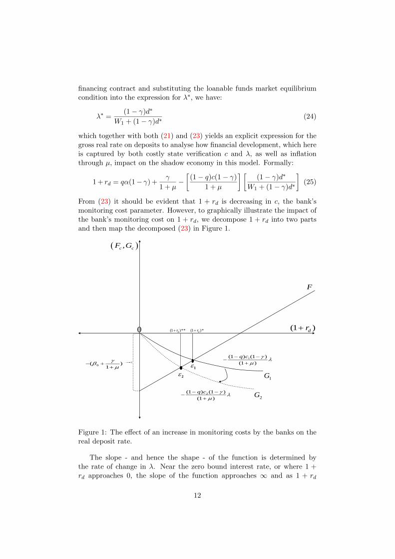
From (23) it should be evident that 1 + rd is decreasing in c, the bank’smonitoring cost parameter. However, to graphically illustrate the impact ofthe bank’s monitoring cost on 1 + rd, we decompose 1 + rd into two partsand then map the decomposed (23) in Figure 1.

0 (1 )dr

F

0( )1

2(1 ) (1 )

(1 )

q c

1(1 ) (1 )

(1 )

q c

1

2

,c cF G

2G

(1 )*dr(1 )**dr

1G

Figure 1: The effect of an increase in monitoring costs by the banks on thereal deposit rate.

The slope - and hence the shape - of the function is determined bythe rate of change in λ. Near the zero bound interest rate, or where 1 +rd approaches 0, the slope of the function approaches ∞ and as 1 + rd

12

approaches ∞, the slope of the function approaches 0. The function istherefore concave, increasing in 1 + rd, but at a decreasing rate.

Here c2 > c1, F is the intercept representation of the function and G1, G2

is the slope representation of 1 + rd corresponding with the increase fromc1 → c2, respectively. As the banks’ monitoring cost increases, there is adownward movement from G1 to G2 as the value of the slope increases.This increase in cost results in a new equilibrium level ε2 which correspondswith the real deposit rate, (1 + rd)

∗∗ which is clearly lower than the initialequilibrium level ε1 which corresponds with the real deposit rate, (1 + rd)

∗.The movement in the results presented here flow in the opposite directionfor any given decrease in c.

The underlying intuition is straightforward: the higher the cost of mon-itoring and the higher the incidence of the stochastic monitoring technologyemployed by the banks, the lower is 1 + rd. Conversely, higher CSV corre-sponds with a lower level of financial development, implying a lower levelof incentives for the depositor to save and hence, a higher incentive for thedepositor to evade in this setting. It is expected that 1 + rd is decreasing inλ, as an increase in the probability (or number of times) that misreportingentrepreneurs can be discovered should lead to an increase in costs for thebank and therefore to a higher CSV altogether.

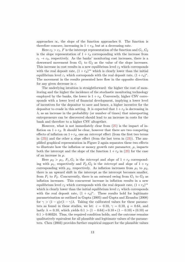
However, what is not immediately clear from (25) is the impact of in-flation on 1 + rd. It should be clear, however that there are two competingeffects of inflation on 1+rd, one an intercept effect (from the first two termsin (23)) and the other a slope effect (from the last term in (23)). The am-plified graphical representation in Figure 2 again separates these two effectsto illustrate how the inflation or money growth rate parameter, µ, impactsboth the intercept and the slope of the function 1 + rd in (23) for the caseof an increase in µ.

Here µ2 > µ1, F1, G1 is the intercept and slope of 1 + rd correspond-ing with µ1, respectively and F2, G2 is the intercept and slope of 1 + rdcorresponding with µ2, respectively. As inflation increases from µ1 to µ2,there is an upward shift in the intercept as the intercept becomes smaller,from F1 to F2. Concurrently, there is an outward swing from G1 to G2 asinflation increases. This concurrent increase in inflation results in a newequilibrium level ε2 which corresponds with the real deposit rate, (1 + rd)

∗∗

which is clearly lower than the initial equilibrium level ε1 which correspondswith the real deposit rate, (1 + rd)

∗. These results hold for legitimateparametrisation as outlined in Gupta (2005) and Gupta and Ziramba (2008)for γ > (1 − q)c(1 − γ)λ. Taking the calibrated values for these parame-ters as found in these studies, we let: c = 0.10, γ = 0.10, q = 0.64, andlastly λ = 0.10, which yields 0.1 > (1 − 0.64) ∗ 0.10 ∗ (1 − 0.10) ∗ (0.10) or0.1 > 0.00324. Thus, the required condition holds, and the outcome remainsqualitatively equivalent for all plausible and legitimate values of the parame-ters. Chen (2003) provides further empirical support for the plausible values

13

0 (1 )dr

2F

1F

0

2

( )1

0

1

( )1

1

(1 ) (1 )

(1 )

q c

2

(1 ) (1 )

(1 )

q c

1

2

,F G

1G

2G

(1 )*dr(1 )**dr

Figure 2: The dual effects of an increase in inflation on the real deposit rate.

of specifically γ and c.These results indicate that as inflation increases the real rate on deposits

decreases, and from ∂β∗

∂rdit would imply that β∗ increases. So, as the depos-

itor in this economy observes a decrease in the real rate on deposits heldat banks, he decides to evade a bigger portion of his income leading to anincrease in the size of β∗. In summary, (21) to (25) and the consequentialanalysis highlights the most important result that emerges from this anal-ysis: that the fraction of income evaded by a depositor depends not onlyon real factors such as tax rates, τ ; penalty rates, θ; and the probability ofgetting caught, (1− σ); but it also hinges critically on the monetary policyparameters in the model, namely the reserve requirement, γ and inflation,π as well as on the bank’s cost parameters, c and λ.

5 The empirical setting

Recent empirical studies focus mainly on real factors as determinants of thesize of the shadow economy. Fishlow and Friedman (1994) find that whencurrent income decreases, tax compliance decreases and hence, the size ofthe shadow economy increases. Scneider (1994) shows how the imposedpenalty rate leads to a higher shadow economy, while Schneider and Enste

14

(2000) argue that the probability of being detected influences the size ofthe shadow economy. Dabla-Norris and Feltenstein (2005) show that theoptimal tax rate may lead to a bigger shadow economy. Dreher, Kotsogiannisand McCorriston (2009) show that improved institutional quality decreasesthe size of the shadow economy and Elgin (2009) further argues that it ispolitical turnover that determines the size of the shadow economy. Onnisand Tirelli (2011) argue that public expenditures decrease the size of theshadow economy, while Cerqueti and Coppier (2011) show how corruptionaffects the shadow economy. Most recently, Alm (2012) states that highertax audit rates may reduce the size of the shadow economy and lastly Boseet al. (2012) provides evidence that it is the level of financial developmentthat determines the size of the shadow economy.

The focal point of a separate strand of the literature is the accuracy ofdifferent measures of the shadow economy. There are various different mea-sures for the shadow economy - some more creative than others - but wewill only highlight the most widely-used measures. Schneider, Buehn andMontenegro (2010) use a Multiple Indicators Multiple Causes (MIMIC) mea-sure, which essentially is a structural equation model (SEM) with one latentvariable. Thiessen (2010) constructs a shadow economy measure based onbehavioural theories and Gomis-Porqueras, Peralta-Alva and Waller (2011)models the shadow economy using a currency demand or money demandapproach. Onnis and Tirelli (2011) suggest using a Modified Total Electric-ity (MTE) approach and more recently, Elgin and Oztunali (2012) use atwo-sector dynamic general equilibrium (DGE) model to obtain the size ofthe shadow economy. It should be mentioned that direct approaches, likesurveys and structured questionnaires, are also widely used to obtain more“direct” measures of the size of the shadow economy.

The essence of our empirical testing however, is based exclusively on ourtheoretical framework.

5.1 Data

The data set used spans the period 1980 - 2009 and includes 150 countries10,constituting a panel data set where N = 150 and T = 30. The period waschosen based on data availability for all key variables, and also to include atleast one high and erratic inflationary period common in our panel - 1980 to1990 - in the empirical analysis. The main variables of interest are discussedbriefly, but we include a detailed description in Table 6 in the Appendix forease of reference.

We compare two measures of the size of the shadow economy. Shadow1is taken from the data set on the size of the shadow economy compiled bySchneider et al. (2010) using the MIMIC estimation method. This measure-

10A list of all the countries included in this analysis is available from the authors.

15

ment covers the period 1999-2007. The second measure, Shadow2 is froma new data set compiled by Elgin and Oztunali (2012)11, where the time-varying size of the shadow economy is estimated using a dynamic generalequilibrium (DGE) model calibrated to a set of macroeconomic variables.This measure covers the period 1950-200912. The correlation coefficient be-tween Shadow1 and Shadow2, as stated in Elgin and Oztunali (2012) andalso verified in this analysis, is 0.987. The strong correlation between thesetwo different measures of the shadow economy, based on different method-ologies over different periods, facilitates balanced results as it excludes theway in which the measurements were calculated as a potential driver of theresults.

Bnkcost is a measure of the banking sector’s average overhead cost,expressed as a percentage of the banking sector’s total assets. Although thismeasure is not only restricted to the bank’s monitoring cost parameter, asdenoted by c in (23) of the theoretical model, by definition it includes c andis proposed here as a rational proxy for c in the absence of a more directand widely available measure of c. This cost measure is also an indication ofthe efficiency with which commercial banks matches surplus units to deficitunits in the economy, and is available from the Financial Structure datasetcompiled and updated by Beck and Demirguc-Kunt (2009). Barth, Caprioand Levine (2002) and Bose et al. (2012) have used Bnkcost as a measureof the inefficiencies in the banking sector.

Infl captures the effect of inflation and is the annual percentage changein consumer prices. As a proxy for inflation, we consider Moneygr which isdefined as the annual growth rate of the M2 monetary aggregate, since insteady state the money growth rate is set equal to the rate of inflation.

Cba, or central bank assets, is defined as the total claims that the centralbank has on the domestic real non-financial sector and is expressed as apercentage of GDP. This variable is included as a relative measure of the sizeof the central bank in the economy and to account for the level of intervention- and the possible effect of financial repression - that economies experience.Curdia and Woodford (2011) extends a standard New Keynesian modeland find central bank assets to be a factor in equilibrium determination.Bernanke and Reinhart (2004) also discuss the importance of central bankbalance sheets and the composition thereof, in effectively implementing newand unconventional balance sheet policies. According to Christiano (2011),

11We gratefully acknowledge the use of the dataset on the shadow economy compiledby Ceyhun Elgin and Oguz Oztunali.

12The econometric literature, in particular on the monetary model of exchange ratedetermination and purchasing power parity, suggests that it is the span of the data, andnot the frequency that enhances econometric analysis of specifically long-run relationshipsbetween macroeconomic variables. This has been shown by Shiller and Perron (1985),Hakkio and Rush (1991), Otero and Simth (2000), Rapach and Wohar (2004) and morerecently by de Bruyn, Gupta and Stander (2013).

16

central bank intervention in asset markets may also prove to be very costly.This may lead to observing a higher overall banking cost in the economy. A’bank balance sheet’ channel for monetary policy through which the centralbank can influence the loan decision of banks, was identified by Chami andCosimano (2010). Through this channel the central bank may influence thebank’s cost functions and ultimately, the decisions of the agent to depositor evade.

The Control variable set includes Gdppc, the real gross domestic product(GDP) per capita. Real GDP is a widely accepted measure of economic de-velopment in the literature (Boyd, Levine and Smith, 2001; Boyd and Jalal,2012) and it may plausibly be used as an indicator of financial developmentsince King and Levine (1993) showed that economic and financial devel-opment are closely related (Boyd and Jalal, 2012). The Control variableset also includes two other important subsets, where the first set measuresthe level of financial development in each country, and comprises of: Dcpb,the domestic credit provided by the banking sector; Prvcrt, the domesticcredit provided by the banking sector as well as other financial institutionsor intermediaries; Intsprd, the interest rate differential between loans anddeposits; M3, the liquid liabilities as a percentage of real GDP and Stmk,a measure of stock market development calculated as the market capitali-sation of all listed companies as a percentage of real GDP. These variablesare often used in the financial development literature as indicators of thedepth and the efficiency of both the banking and the financial sector (Kingand Levine, 1993; Levine and Zervos, 1998; Levine, Loayza and Beck, 2000;Boyd et al. 2001; Barth et al. 2002 and Boyd and Jalal, 2012). From thesevariables, we construct two financial development indicators using principalcomponents analysis (PCA) and extract the unobserved common factors ofthese variables.

We define Findev as the first proxy for financial development and itconsists of the first principal component of the log-levels of Dcpb, Prvcrt,M3 and Stmk which accounts for 80% of the variation in these four vari-ables. We define the second proxy for financial development as Findev2,which consists of the first principal component of the log-levels of Dcpb,Prvcrt and Intsprd and it accounts for 68% of the variation in these threevariables. Intsprd is defined as the lending interest rate minus the depositinterest rate as published by the World Bank, and it indicates the magni-tude of the wedge that financial repression induces between the interest ratesthat banks charge on loans and the interest rate banks offer on deposits13.This additional second proxy for financial development, given that Gdppcis already a viable alternative to our first proxy, Findev, is an attempt tofollow the recommendations of Levine (2005) and Boyd and Jalal (2012)

13Gupta (2005) provides a clear theoretical explanation of the characteristics of financialrepression through obligatory high reserve requirements set by monetary authorities.

17

that empirical measures of financial development should directly measurefinancial functions performed by the financial system. The PCA allows usto reduce the dimensionality of the set of variables to be included in ourempirical analysis, whilst still retaining most of the informational contentoffered by these same variables (Bittencourt, 2012). It also aids in ensuringa more stable computational environment (Jolliffe, 1982).

The second subset measures the broad institutional quality of each coun-try, and comprises of: Regquality, regulatory quality captures the percep-tion of the ability of the government to formulate and implement soundpolicies and regulations that would permit and promote private sector de-velopment; Ruleoflaw captures the perception of the extent to which agentshave confidence in and abide by the rules of their respective society, in partic-ular the quality of contract enforcement, property rights, the police and thecourts, as well as the likelihood of crime and violence and Fiscfreed mea-sures fiscal freedom, or the extent of a country’s total tax burden. All threethese variables are compiled as indices, with higher values of the index cor-responding to better governance and a lower tax burden, respectively. Thesevariables are commonly used in the shadow economy literature as importantindicators of the policy, institutional and regulatory environment which im-pacts on the size of the shadow economy observed in countries (Schneider,2007; Bose et al. 2012). Data on both Regquality and Ruleoflaw is fromthe World Governance Indicators (WGI) dataset maintained by the WorldBank and covers the period 1996-2009, and Fiscfreed is found in the In-dex of Economic Freedom dataset compiled by The Heritage Foundationand covers the period 1995-2009. All other data is taken from the WorldDevelopment Indicators and Global Development Finance (WDI) datasetpublished by the World Bank.

We again employ PCA to construct a proxy for the institutional, regu-latory and policy strength of the countries in our sample. Instit is the firstprincipal component of the levels of Regquality, Ruleoflaw and Fiscfreedand accounts for 66% of the total variation in these three variables. There isstrong consensus in the literature on the shadow economy that institutionsare very important in depressing the size of the shadow economy14.

All main variables are expressed in logarithmic form. This is consis-tent with the depositor’s life-time log-utility function, and as detailed in deBruyn, Gupta and Stander (2013) this also allows more accurate analysis ofthe relative effect of the change in one variable on the change in another,which here is the relative effect of both financial development and inflationon the size of the shadow economy.

Table 1 illustrates the behaviour of the variables of interest, Moneygr

14In different economic settings, Koreshkova (2006), Dreher, Kotsogiannis and McCor-riston (2009), Elgin (2009) as well as Onnis and Tirelli (2011) all produce results support-ing the attenuating effect of good institutions on the size of the shadow economy.

18

and Bnkcost over the sample period. The mean of Moneygr for the sampleis 44.3 percent annually, while the mean of Bnkcost for the sample is 0.044,or 4.4 percent of the total value of the bank’s assets. The values of thevariables are aggregated over each year to calculate the mean. The differencebetween the minimum and maximum value of most of the variables confirmsthe observed variability in a heterogeneous panel of countries, such as theone presented here.

<<< Table 1 about here >>>

We also provide the correlation matrix of the two main explanatory andother control variables on the size of the shadow economy in Table 2.

<<< Table 2 about here >>>

Firstly, there is a strong positive correlation between the two measures ofthe shadow economy, confirming the findings in Elgin and Oztunali (2012).Both our variables of interest, Bnkcost and Moneygr, are positively corre-lated with both measures of the shadow economy, Shadow1 and Shadow2as expected. Financial development seems to have the expected attenuatingeffect on the size of the shadow economy, as does the level of and the relativechange in the level of institutional quality. Gdppc is negatively correlated tothe shadow economy, implying that societies that are more developed bothfinancially and economically seems to be engaging less in underground eco-nomic activity. Lastly, Cba is positively correlated to the shadow economy,and negatively correlated to both measures of financial development, insti-tutional quality and Gdppc. This suggests that the size of total claims thecentral bank has over the real domestic non-financial sector, or the strongerthe ability of the central bank to intervene in the market, the more adverseconditions these markets face in general.

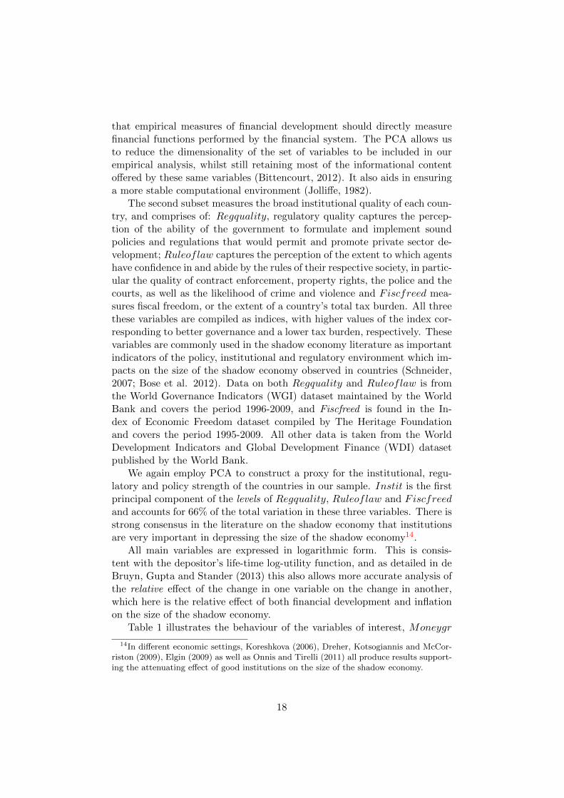
We also present the simple ordinary least squares (OLS) regression linesbetween our variables of interest and the size of the shadow economy inFigure 3, where we plot country-specific paired observations of the means(aggregated over countries) of both Moneygr and the log-level of Bnkcostagainst the log-level of the shadow economy.

Note the positive relationship between banking cost and money growthon the shadow economy for country-specific observations15. From the ob-served data, it would seem that higher (lower) values of banking cost andhigher (lower) values of the money growth rate, both correspond with higher(lower) values of the size of the shadow economy increases. Therefore - with-out implying causality at this stage - there seems to be some basis for our

15Both these positive relationships hold even when we use the short-span measure ofthe shadow economy, Shadow1 as well as for paired observations over the whole sampleperiod.

19

-2.5

-2-1

.5-1

-.5

countr

y m

log_shadow

2

-5 -4 -3 -2country mlog_bnkcost

OLS Fitted Line

-2.5

-2-1

.5-1

-.5

countr

y m

log_shadow

2

0 50 100 150 200country m_moneygr

OLS Fitted Line

Figure 3: OLS regression lines of the log-levels of Banking Cost and MoneyGrowth on the Shadow Economy in each country for 1980-2009, respectively.

a priori expectation and predictions of our theoretical model, that both cand µ are positive with respect to the size of the shadow economy.

5.2 The empirical methodology employed

Since we have an unbalanced panel of observations from countries (N = 150)spanning multiple years (T = 30), and it is clear that there is some persis-tence in some of our variables of interest, we make use of dynamic panel(time-series) data analysis. The dynamic panel methodology allows usto deal more effectively with econometric problems like non-stationarity,joint statistical and economic endogeneity, potential simultaneity bias, un-observed country-specific effects that may lead to omitted variable bias andimportantly, measurement error. We are analysing the unobserved economyand as such measurement error is implied. This methodology also exploresthe added information from the time dimension in order to yield more ac-curate and informative estimates. Following Aghion, Bacchetta, Rancie andRogoff (2009), we use the general method of moments (GMM) dynamicpanel data estimator developed in Arellano and Bond (1991), Arellano andBover(1995) and more specifically, the system GMM estimator developedin Blundell and Bond(1998). We compute Windmeijer-corrected two-stepstandard errors following the methodology proposed by Windmeijer (2005).This system GMM estimator addresses the aforementioned econometric is-sues in a dynamic formulation, where the lagged variable of the dependentvariable is added to account for the persistence observed in the data16.

We also expect our panel to be heterogeneous due to the inclusion ofsuch a large number of countries with different economic, legal and regula-

16Roodman (2009) offers a step-by-step pedagogical account of the use of GMM styleestimators.

20

tory policies, different political dispensations, different social issues whichincludes different levels of income inequality and different levels of both fi-nancial development and economic development. Moreover, the countriesin our sample also share certain similar characteristics, like banking insti-tutions, common monetary areas, trade agreements, monetary authoritiesand in some instances similar rules dictating their participation in the globaleconomy. Our preferred estimator accounts for both scenarios.

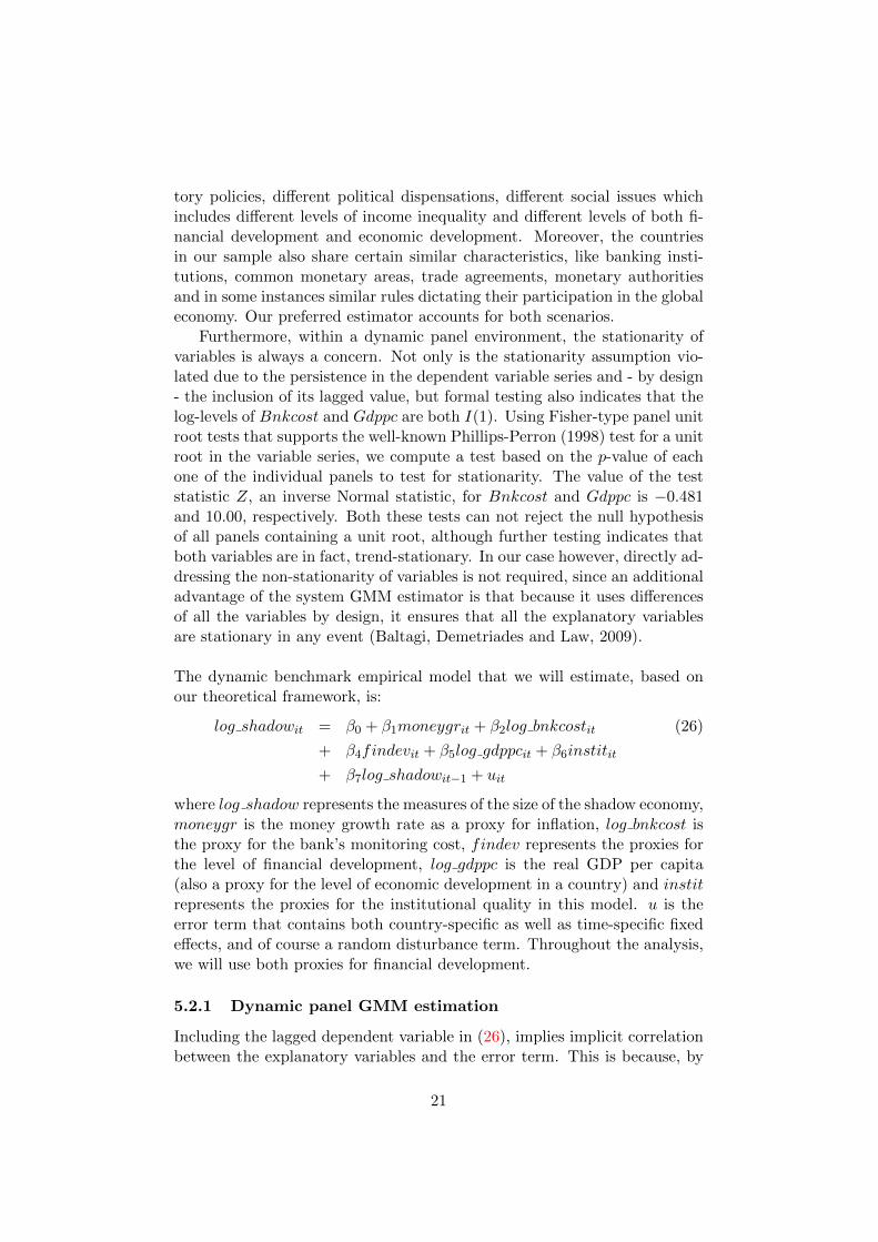
Furthermore, within a dynamic panel environment, the stationarity ofvariables is always a concern. Not only is the stationarity assumption vio-lated due to the persistence in the dependent variable series and - by design- the inclusion of its lagged value, but formal testing also indicates that thelog-levels of Bnkcost and Gdppc are both I(1). Using Fisher-type panel unitroot tests that supports the well-known Phillips-Perron (1998) test for a unitroot in the variable series, we compute a test based on the p-value of eachone of the individual panels to test for stationarity. The value of the teststatistic Z, an inverse Normal statistic, for Bnkcost and Gdppc is −0.481and 10.00, respectively. Both these tests can not reject the null hypothesisof all panels containing a unit root, although further testing indicates thatboth variables are in fact, trend-stationary. In our case however, directly ad-dressing the non-stationarity of variables is not required, since an additionaladvantage of the system GMM estimator is that because it uses differencesof all the variables by design, it ensures that all the explanatory variablesare stationary in any event (Baltagi, Demetriades and Law, 2009).

The dynamic benchmark empirical model that we will estimate, based onour theoretical framework, is:

log shadowit = β0 + β1moneygrit + β2log bnkcostit (26)

+ β4findevit + β5log gdppcit + β6institit

+ β7log shadowit−1 + uit

where log shadow represents the measures of the size of the shadow economy,moneygr is the money growth rate as a proxy for inflation, log bnkcost isthe proxy for the bank’s monitoring cost, findev represents the proxies forthe level of financial development, log gdppc is the real GDP per capita(also a proxy for the level of economic development in a country) and institrepresents the proxies for the institutional quality in this model. u is theerror term that contains both country-specific as well as time-specific fixedeffects, and of course a random disturbance term. Throughout the analysis,we will use both proxies for financial development.

5.2.1 Dynamic panel GMM estimation

Including the lagged dependent variable in (26), implies implicit correlationbetween the explanatory variables and the error term. This is because, by

21

inclusion, the lagged shadow economy depends on uit−1 which contains thecountry-specific and time-specific effects. This further supports the choiceof our preferred estimator suggested by Blundell and Bond (1998), whichbasically differences the model to get rid of country specific effects or anytime-invariant country specific variable.

The moment conditions utilize the orthogonality conditions between thedifferenced errors and lagged values of the dependent variable. This assumesthat the random disturbances term contained in uit, are serially uncorre-lated. We compute two diagnostic tests using the GMM procedure to testfor first order and second order serial correlation in the disturbances. For va-lidity, one should reject the null of the absence of first order serial correlationand not reject the null of the absence of second order serial correlation.

The dynamic system GMM estimation treats all the variables - otherthan the lagged dependent variable - as if they were either strictly exogenousor predetermined but not strictly exogenous, in that it assumes these vari-ables are uncorrelated with the random disturbances in uit. As cautiouslystated in Baltagi et al. (2009), the differencing performed by the systemGMM estimator may also remove any correlation due to the time-invariantcommon factors. An additional advantage of the system GMM estimatoris that it does not “difference away” the fixed effects, but it instrumentsfor the lagged dependent variable and other explanatory variables that maystill be correlated with the disturbances by other variables believed to beuncorrelated with these fixed effects.

5.3 Empirical results

The two-step system GMM results reported in Table 3 provides encour-aging support for the developed theoretical model. The recommendationsof Roodman (2009) are followed and a detailed description of the differentspecification and instrument sets are provided first before the results arediscussed. For the results in Table 3, we use the maximum number of in-struments that the GMM procedure allows and that are available in thedataset.

<<< Table 3 about here >>>

For columns (1) to (3), the endogenous (predetermined) or internal in-strument set consists only of log bnkcost and the lagged dependent variable.The external instrument set consists of log cba, log intsprd and the time-dummies for column (1); log cba and the time-dummies for column (2) andonly the time-dummies for column (3), respectively. This was done to reducethe instrument count and avoid proliferation of instruments. All instrumentsets are valid, as supported by the Sargan statistic, where the hypothesiscannot be rejected that the instruments are exogenous. Moreover, the in-strument count is always considerably less than the number of observations.

22

The Arellano-Bond autocorrelation test also indicates that there is no serialcorrelation in the idiosyncratic disturbance term.

To account for the suspected economic endogeneity between Moneygrand Findev in a direct way, columns (1) to (3) exclude both principal com-ponents measures of financial development. In columns (4) to (6), boththe different measures of financial development is included separately. Ex-cept for column (1), the forward orthogonal deviations transformation firstsuggested in Arellano and Bover (1995), are used as an alternative to thestandard differencing. This transformation has the advantage of preservingsample size when the selected panel has gaps, or is unbalanced. All specifica-tion reported in Table 3 allow for the idiosyncratic disturbances to be bothheteroskedastic as well as correlated within countries, but not across coun-tries. Finite-sample Windmeijer (2005) corrected robust errors are reportedin all columns.

The estimation performed in column (4) treats log bnkcost, Findev andthe lagged dependent variable of the shadow economy as endogenous, andtherefore uses the second and deeper lagged values of these variables asinternal instruments for the differenced equation and the first and deeperlagged differenced values as instruments for the level equation. The size ofthe central bank, the interest rate spread and the time-dummies are treatedas exogenous and therefore used as external instruments for the equationin levels. For column (5), Findev is considered to be only predeterminedand thus the first and earlier lagged values are used as instruments for thetransformed equation and the difference of Findev for the equation in levels.The external (or exogenous) instrument set remains the same. In column(6), the second measure of financial development is again treated as an en-dogenous variable and included in the internal set together with log bnkcostand l.log shadow2. The exogenous instrument set used in column (6) nowexcludes the interest rate spread, as this forms part of Findev2.

Bnkcost estimates reported are positive and significant for all specifiedsystem GMM estimations. The size of the coefficients range from 0.00515 to0.00872 and is in line with estimates obtained using the fixed effects (FE)estimator17. These results indicate that an increase of 1% in banking cost,would likely lead to an additional 0.5% − 0.9% increase in the size of theshadow economy, suggesting that as banks face an increasingly costly stateverification problem, the decision of the agents would lean more towardsevading a bigger portion of their income and hence we observe an increasein the size of the shadow economy. In the sample countries examined here,a 1% increase in banking cost would add almost $2 billion to the shadoweconomy on average as the mean value of GDP for these countries is $200

17The GMM results accord well with results obtained from fixed effects (FE) estimations,which serve as a consistency check. The FE results are provided in the Appendix in Table5.

23

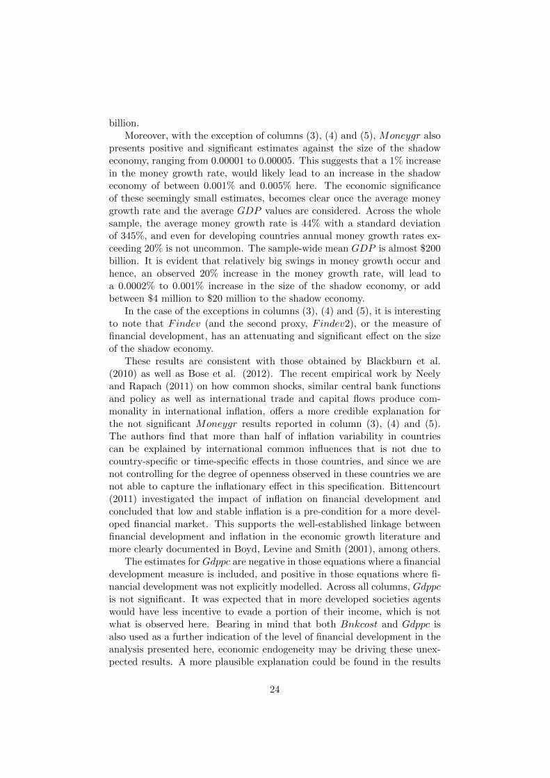
billion.Moreover, with the exception of columns (3), (4) and (5), Moneygr also

presents positive and significant estimates against the size of the shadoweconomy, ranging from 0.00001 to 0.00005. This suggests that a 1% increasein the money growth rate, would likely lead to an increase in the shadoweconomy of between 0.001% and 0.005% here. The economic significanceof these seemingly small estimates, becomes clear once the average moneygrowth rate and the average GDP values are considered. Across the wholesample, the average money growth rate is 44% with a standard deviationof 345%, and even for developing countries annual money growth rates ex-ceeding 20% is not uncommon. The sample-wide mean GDP is almost $200billion. It is evident that relatively big swings in money growth occur andhence, an observed 20% increase in the money growth rate, will lead toa 0.0002% to 0.001% increase in the size of the shadow economy, or addbetween $4 million to $20 million to the shadow economy.

In the case of the exceptions in columns (3), (4) and (5), it is interestingto note that Findev (and the second proxy, Findev2), or the measure offinancial development, has an attenuating and significant effect on the sizeof the shadow economy.

These results are consistent with those obtained by Blackburn et al.(2010) as well as Bose et al. (2012). The recent empirical work by Neelyand Rapach (2011) on how common shocks, similar central bank functionsand policy as well as international trade and capital flows produce com-monality in international inflation, offers a more credible explanation forthe not significant Moneygr results reported in column (3), (4) and (5).The authors find that more than half of inflation variability in countriescan be explained by international common influences that is not due tocountry-specific or time-specific effects in those countries, and since we arenot controlling for the degree of openness observed in these countries we arenot able to capture the inflationary effect in this specification. Bittencourt(2011) investigated the impact of inflation on financial development andconcluded that low and stable inflation is a pre-condition for a more devel-oped financial market. This supports the well-established linkage betweenfinancial development and inflation in the economic growth literature andmore clearly documented in Boyd, Levine and Smith (2001), among others.

The estimates for Gdppc are negative in those equations where a financialdevelopment measure is included, and positive in those equations where fi-nancial development was not explicitly modelled. Across all columns, Gdppcis not significant. It was expected that in more developed societies agentswould have less incentive to evade a portion of their income, which is notwhat is observed here. Bearing in mind that both Bnkcost and Gdppc isalso used as a further indication of the level of financial development in theanalysis presented here, economic endogeneity may be driving these unex-pected results. A more plausible explanation could be found in the results

24

for the institutional framework. Instit estimates are negative and significantthroughout the specification (with the exception of column (5)), but highlysignificant once the measures of financial development were not included.These results coalesce with the findings of Koreshkova (2006), Elgin (2009)and Onnis and Tirelli (2011), among others. In this empirical setting, it isclearly institutions and the level of financial development that impacts onthe size of the shadow economy, and not the per capita income levels or thelevel of economic development.

The lagged dependent variable is positive and significant in all specifi-cation, as expected from the persistent nature of the shadow economy. Thesize of the lagged coefficient in most columns is high, again raising concernsabout non-stationarity and hence, spurious regression results. In simulationstudies, performed by Blundell, Bond and Windmeijer (2001), the efficiencyand bias of system GMM estimates are compared to other estimators inthe presence of highly persistent series, and found to improve upon boththe precision and finite sample bias of other estimates. Moreover, Phillipsand Moon (1999) formalised the idea that the cross-sectional informationadded in a panel framework provides more information, and therefore aclearer signal about the average long-run relation parameter, or the coeffi-cient of the lagged dependant variable. Phillips and Moon (1999) providepanel asymptotic theory which shows that the estimate for the coefficienton the lagged variable is consistent for persistent series, and hence spuriousregression results in a non-stationary panel analysis is less problematic.

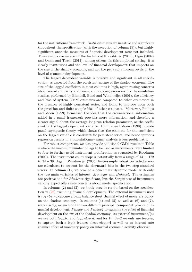
For robust comparison, we also provide additional GMM results in Table4 where the maximum number of lags to be used as instruments, were limitedto four to further avoid instrument proliferation as suggested by Roodman(2009). The instrument count drops substantially from a range of 141− 172to 34− 39. Again, Windmeijer (2005) finite-sample robust corrected errorsare calculated to account for the downward bias in the two-step standarderrors. In column (1), we provide a benchmark dynamic model with onlythe two main variables of interest, Moneygr and Bnkcost. The estimatesare positive and for Bbnkcost significant, but the Sargan test of instrumentvalidity expectedly raises concerns about model specification.

In columns (2) and (3), we firstly provide results based on the specifica-tion in (26) excluding financial development. The external instrument usedis log cba, to capture a bank balance sheet channel effect of monetary policyon the shadow economy. In columns (4) and (5) as well as (6) and (7),respectively, we include the two different principal component proxies of fi-nancial development, Findev and Findev2 to examine the effect of financialdevelopment on the size of the shadow economy. As external instrument/(s)we use both log cba and log intsprd, and for Findev2 we only use log cba,to capture both a bank balance sheet channel as well as an interest ratechannel effect of monetary policy on informal economic activity observed.

25

<<< Table 4 about here >>>

The estimates reported for Bnkcost are all positive and almost alwayssignificant. The range of the coefficient estimates are 0.0111 to 0.0222. Onaverage, a 1% increase in banking cost would lead to a 1% to 2% increasein the size of the shadow economy, or add between $2 billion to $4 billion tothe shadow economy. These estimates, although more pronounced here, arein line with the previous GMM results as well as the FE results in Table 5.

Moneygr estimates reported are mostly positive and either significantor marginally not significant (columns (2) and (3)). The range of coeffi-cient estimates are between 0.0000005 and 0.0001. At the upper end of therange, this would again imply that a 20% increase in the money growthrate would lead to a 0.2% increase in the shadow economy, which translatesto an additional $500 million of informal economic activity. These resultsare also broadly in line with the previous GMM estimates and the FE es-timates. It should be noted that the only exception, a negative coefficientestimate reported in column (4), was based on modelling the money growthrate as endogenous to the model, and the result obtained would suggestthat the money growth rate does not introduce endogeneity in our specifiedmodel in (26). Besides, the use of the lagged values of the level variablesas instruments for the transformed equation and the lagged values of thefirst differences as instruments for the equation in levels, already adequatelydeals with any suspected endogeneity, as further explained in Kose, Prasadand Taylor (2011).

We also report two-stage FE results in Table 5 in the Appendix, firstlyfor the whole sample following the recommendations of Judson and Owen(1999), and then using sub-samples of OECD and Latin American countries.Owning to the long sample period (T = 30), the Nickell (1981) bias is oforder O(1/T ) and hence, presents less of a problem than what is observedin typically shorter time-series panels. Moreover, we supplement the FE es-timation by including exogenous regressors through the use of instrumentalvariables which is not only consistent with our preferred GMM estimator,but also more closely represent the indirect correspondence of our main vari-ables of interest with the shadow economy, evident from (21), (22) and (25).For the full sample, log cba and log intsprd are again used to capture botha bank balance sheet channel effect as well as an interest rate channel effectof monetary policy on the size of the shadow economy. For the respectivesub-samples of both OECD and Latin American countries, Domsave is usedas an instrument to capture the savings decisions of agents in this specifi-cation. Domsave is gross domestic savings, expressed as a percentage ofGDP .

The FE results obtained are broadly in line with the GMM results pre-sented herein. Bnkcost is almost always positive, yet not significant. Thepositive Moneygr estimates are significant, and apply to the benchmark

26

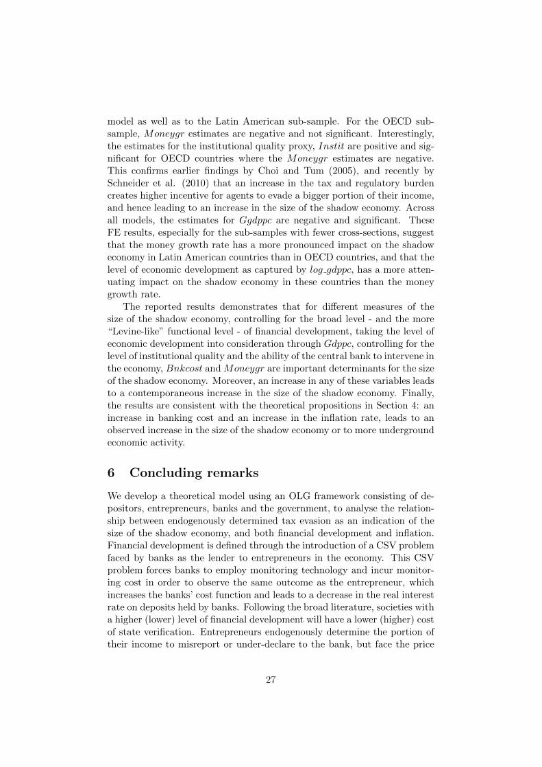
model as well as to the Latin American sub-sample. For the OECD sub-sample, Moneygr estimates are negative and not significant. Interestingly,the estimates for the institutional quality proxy, Instit are positive and sig-nificant for OECD countries where the Moneygr estimates are negative.This confirms earlier findings by Choi and Tum (2005), and recently bySchneider et al. (2010) that an increase in the tax and regulatory burdencreates higher incentive for agents to evade a bigger portion of their income,and hence leading to an increase in the size of the shadow economy. Acrossall models, the estimates for Ggdppc are negative and significant. TheseFE results, especially for the sub-samples with fewer cross-sections, suggestthat the money growth rate has a more pronounced impact on the shadoweconomy in Latin American countries than in OECD countries, and that thelevel of economic development as captured by log gdppc, has a more atten-uating impact on the shadow economy in these countries than the moneygrowth rate.

The reported results demonstrates that for different measures of thesize of the shadow economy, controlling for the broad level - and the more“Levine-like” functional level - of financial development, taking the level ofeconomic development into consideration through Gdppc, controlling for thelevel of institutional quality and the ability of the central bank to intervene inthe economy, Bnkcost and Moneygr are important determinants for the sizeof the shadow economy. Moreover, an increase in any of these variables leadsto a contemporaneous increase in the size of the shadow economy. Finally,the results are consistent with the theoretical propositions in Section 4: anincrease in banking cost and an increase in the inflation rate, leads to anobserved increase in the size of the shadow economy or to more undergroundeconomic activity.

6 Concluding remarks

We develop a theoretical model using an OLG framework consisting of de-positors, entrepreneurs, banks and the government, to analyse the relation-ship between endogenously determined tax evasion as an indication of thesize of the shadow economy, and both financial development and inflation.Financial development is defined through the introduction of a CSV problemfaced by banks as the lender to entrepreneurs in the economy. This CSVproblem forces banks to employ monitoring technology and incur monitor-ing cost in order to observe the same outcome as the entrepreneur, whichincreases the banks’ cost function and leads to a decrease in the real interestrate on deposits held by banks. Following the broad literature, societies witha higher (lower) level of financial development will have a lower (higher) costof state verification. Entrepreneurs endogenously determine the portion oftheir income to misreport or under-declare to the bank, but face the price

27

of doing so in the form of higher costs for access to and conditions of ob-taining credit. These higher costs, or lower real rate on deposits and hencea lower level of financial development, provides an incentive to depositors toparticipate in tax-evasion activities as the marginal benefit of tax evasion isat least equal to the marginal cost thereof.

The empirical results provide consistent support for the theoretical find-ings. Once the level of both economic development and institutional qualityis accounted for, concurrent with the size of the central bank and hence itsability to intervene in the economy, the reported estimates are evident of thefact that lower (higher) levels of financial development and higher (lower)inflation causes a bigger (smaller) shadow economy. Thus from a policyperspective, the role of financial development and lower rates of inflation incurbing the size of shadow economy is of paramount importance.

28

References

Aghion, P., Bacchetta, P., Ranciere, R. and Rogoff, K.: 2009, Exchangerate volatility and productivity growth: The role of financial development,Journal of Monetary Economics 56, 494–513.

Alm, J.: 2012, Measuring, explaining, and controlling tax evasion: lessonsfrom theory, experiments, and field studies, International Tax and PublicFinance 19, 54–77.

Arana, O. M. V.: 2004, Economic growth and the household optimal in-come tax evasion. Discussion Paper No. 275, Department of Economics,Universidad Nacionale de Colombia.

Arellano, M. and Bond, S.: 1991, Some tests of specification for panel data:Monte Carlo evidence and an application to employment equations, Re-view of Economic Studies 58, 277–297.

Arellano, M. and Bover, O.: 1995, Another look at the instrumental-variable estimation of error-components models, Journal of Econometrics68, 29–51.

Atolia, M.: 2003, An OLG model of tax evasion with public capital. Workingpaper, Department of Economics, Florida State University, Tallahassee,FL., USA.

Atolia, M.: 2009, Tax evasion in an overlapping generations model withpublic investment. Working paper, Department of Economics, FloridaState University, Tallahassee, FL., USA.

Baltagi, B. H., Demetriades, P. O. and Law, S. H.: 2009, Financial develop-ment and openness: Evidence from panel data, Journal of DevelopmentEconomics 89, 285–296.

Barth, J. R., Caprio, G. J. and Levine, R.: 2004, Bank regulation and super-vision: what works best?, Journal of Financial Intermediation 13(2), 205–248.

Beck, T. and Demirguc-Kunt, A.: 2009, Financial institutions and marketsacross countries and over time: Data and analysis. World Bank PolicyResearch Working Paper No. 4943.

Bernanke, B. and Gertler, M.: 1989, Agency costs, net worth and businessfluctuations, American Economic Review 79(1), 14–31.

Bernanke, B. S. and Reinhart, V. R.: 2004, Conducting monetary policyat very low short-term interest rates, The American Economic Review94(2), 85–90.

29

Bittencourt, M.: 2011, Inflation and financial development: Evidence fromBrazil, Economic Modelling 28(1-2), 91–99.

Bittencourt, M.: 2012, Financial development and economic growth in LatinAmerica: Is Schumpeter right?, Journal of Policy Modeling 34(3), 341–355.

Blackburn, K., Bose, N. and Capasso, S.: 2010, Tax evasion, the under-ground economy and financial development. Discussion Paper No. 138,Centre for Growth and Business Cycle Research, Economic Studies, Uni-versity of Manchester, Manchester, UK.

Blundell, R. and Bond, S.: 1998, Initial conditions and moment conditionsin dynamic panel data models, Journal of Econometrics 87, 115–143.

Blundell, R., Bond, S. and Windmeijer, F.: 2001, Nonstationary Panels,Panel Cointegration, and Dynamic Panels (Advances in Econometrics),Vol. 15, Emerald Group Publishing Limited, chapter Estimation in dy-namic panel data models: Improving on the performance of the standardGMM estimator, pp. 53–91.

Bose, N., Capasso, S. and Wurm, M. A.: 2012, The impact of banking de-velopment on the size of shadow economies, Journal of Economic Studies39(6), 620–638.

Boyd, J. H. and Jalal, A. M.: 2012, A new measure of financial development:Theory leads measurement, Journal of Development Economics 99, 341–357.

Boyd, J. H., Levine, R. and Smith, B. D.: 2001, The impact of inflation onfinancial sector performance, Journal of Monetary Economics 47, 221–248.

Bryant, J. and Wallace, N.: 1980, Open market operations in a model of reg-ulated, insured intermediaries, Journal of Political Economy 88(1), 146–173.

Cerqueti, R. and Coppier, R.: 2011, Economic growth, corruption and taxevasion, Economic Modelling 28, 489–500.

Chami, R. and Cosimano, T. F.: 2010, Monetary policy with a touch ofBasel, Journal of Economics and Business 62(3), 161–175.

Chen, B.-L.: 2003, Tax evasion in a model of endogenous growth, Review ofEconomic Dynamics 6, 381–403.

Choi, J. P. and Thum, M.: 2005, Corruption and the shadow economy,International Economic Review 46(3), 817–836.

30

Christiano, L.: 2011, Remarks on unconventional monetary policy, Interna-tional Journal of Central Banking 7(1), 121–130.

Curdia, V. and Woodford, M.: 2011, The central-bank balance sheet as aninstrument of monetary policy, Journal of Monetary Economics 58(1), 54–79.

Dabla-Norris, E. and Feltenstein, A.: 2005, The underground economy andits macroeconomic consequences, The Journal of Policy Reform 8(2), 153–174.

de Bruyn, R., Gupta, R. and Stander, L.: 2013, Testing the monetary modelfor exchange rate determination in South Africa: Evidence from 101 yearsof data, Contemporary Economics 7(1), 5–18.

DelMonte, A. and Papagni, E.: 2001, Public expenditure, corruption, andeconomic growth: the case of Italy, European Journal of Political Economy17, 1–16.

Di Giorgio, G.: 1999, Financial development and reserve requirements, TheJournal of Banking and Finance 23, 1031–1041.

Dreher, A., Kotsogiannis, C. and McCorriston, S.: 2009, How do institutionsaffect corruption and the shadow economy?, International Tax and PublicFinance 16, 773–796.

Elgin, C.: 2009, Political turnover, taxes and the shadow economy. JobMarket paper, Department of Economics, University of Minnesota, MN.,USA.

Elgin, C. and Oztunali, O.: 2012, Shadow economies around the world:Model based estimates. Working Papers 2012/05, Bogazici University,Department of Economics, Turkey.

Fishlow, A. and Friedman, J.: 1994, Tax evasion, inflation and stabilisation,Journal of Development Economics 43, 105–123.

Gomis-Porqueras, P., Peralta-Alva, A. and Waller, C.: 2011, Quantifyingthe shadow economy: Measurement with theory. Working Paper 2011-015A.

Gupta, R.: 2005, Costly state monitoring and reserve requirements, Annalsof Economics and Finance 6(2), 263–288.

Gupta, R.: 2008, Tax evasion and financial repression, Journal of Economicsand Business 60, 517–535.

31

Gupta, R. and Ziramba, E.: 2009, Tax evasion and financial repression: areconsideration using endogenous growth models, Journal of EconomicStudies 36(6), 660–674.

Gupta, R. and Ziramba, E.: 2010, Misalignment in the growth-maximizingpolicies under alternative assumptions of tax evasion, The Journal of Ap-plied Business Research 26(3), 69–80.

Hakkio, C. S. and Rush, M.: 1991, Co-integration: how short is the longrun?, Journal of International Money and Finance 10(4), 571–581.

Holman, J. A. and Neanidis, K. C.: 2006, Financing government expendi-ture in an open economy, Journal of Economic Dynamics and Control30(8), 1315–1337.

Hugo, V.: 1862, Les Miserables, Kelmscott Society, New York.

Jolliffe, I. T.: 1982, A note on the use of principal components in regression,Journal of the Royal Statistical Society 31(3), 300–303. Series C - AppliedStatistics).

Judson, R. A. and Owen, A. L.: 1999, Estimating dynamic panel datamodels: a guide for macroeconomists, Economics Letters 65(1), 9–15.

King, R. and Levine, R.: 1993, Capital markets and financial intermedi-ation, Cambridge University Press, Cambridge, UK, chapter Financialintermediation and economic development.

Koreshkova, T. A.: 2006, A quantitative analysis of inflation as a tax on theunderground economy, Journal of Monetary Economics 53, 773–796.

Kose, A. M., Prasad, E. S. and Taylor, A. D.: 2011, Thresholds in the processof international financial integration, Journal of International Money andFinance 30(1), 147–179.

Levine, R.: 2005, Handbook of Economic Growth, chapter Finance andGrowth: Theory and Evidence, p. 865–934.

Levine, R., Loayza, N. and Beck, T.: 2000, Financial intermediation andgrowth: Causality and causes, Journal of Monetary Economics 46, 31–77.

Levine, R. and Zervos, S. J.: 1998, Stock markets, banks, and economicgrowth, The American Economic Review 88, 537–558.

Lucas Jr., R. E.: 1976, Econometric policy evaluation: A critique, Carnegie-Rochester conference series on public policy, Vol. 1, North-Holland,pp. 19–46.

32

Myerson, R.: 1979, Incentive-compatibility and the bargaining problem,Econometrica 47, 61–73.

Neely, C. J. and Rapach, D. E.: 2011, International comovements in inflationrates and country characteristics, Journal of International Money andFinance 30, 1471–1490.

Nickell, S.: 1981, Biases in dynamic models with fixed effects, Econometrica49(6), 1417–1426.

Onnis, L. and Tirelli, P.: 2011, Institutions, policies and economic develop-ment. what are the causes of the shadow economy? Working paper seriesNo. 206.

Otero, J. and Smith, J.: 2000, Testing for co-integration: power versusfrequency of observation - further Monte-Carlo results, Economics Letters67(1), 5–9.

Phillips, P. C. and Moon, H. R.: 1999, Linear regression limit theory andnonstationary panel data, Econometrica 67(5), 1057–1111.

Phillips, P. C. and Perron, P.: 1988, Testing for a unit root in time seriesregression, Biometrika 75, 335–346.

Rapach, D. E. and Wohar, M. E.: 2004, Testing the monetary model ofexchange rate determination: a closer look at panels, Journal of Interna-tional Money and Finance 23(6), 867–895.

Roodman, D.: 2009, How to do xtabond2: An introduction to differenceand system GMM in Stata, Stata Journal 9(1), 86–136.

Roubini, N. and Sala-i-Martin, X.: 1995, A growth model of inflation,tax evasion, and financial repression, Journal of Monetary Economics35, 275–301.

Sandmo, A.: 2012, An evasive topic: theorizing about the hidden economy,International Tax and Public Finance 19, 5–24.

Schneider, F.: 1994, Essays on Economic Psychology, Springer PublishingCompany, Berlin, Heidelberg, Germany, chapter Measuring the size anddevelopment of the shadow economy. Can the causes be found and theobstacles be overcome?, pp. 193–212.

Schneider, F.: 2007, Shadow economies and corruption all over the world:new estimates for 145 countries, Economics 9.

Schneider, F., Buehn, A. and Montenegro, C. E.: 2010, New estimates forthe shadow economies all over the world, International Economic Journal24(4), 443–461.

33

Schneider, F. and Enste, D.: 2000, Shadow economies: sizes, causes andconsequences, Journal of Economic Perspectives 38, 77–114.

Shiller, R. J. and Perron, P.: 1985, Testing the random walk hypothesis:Power versus frequency of observation, Economics Letters 18(4), 381–386.

Thießen, U.: 2010, The shadow economy in international comparison: Op-tions for economic policy derived from an OECD panel analysis, Interna-tional Economic Journal 24(4), 481–5091.

Windmeijer, F.: 2005, A finite sample correction for the variance of lineartwo-step GMM estimator, Journal of Econometrics 126(1), 25–51.

34

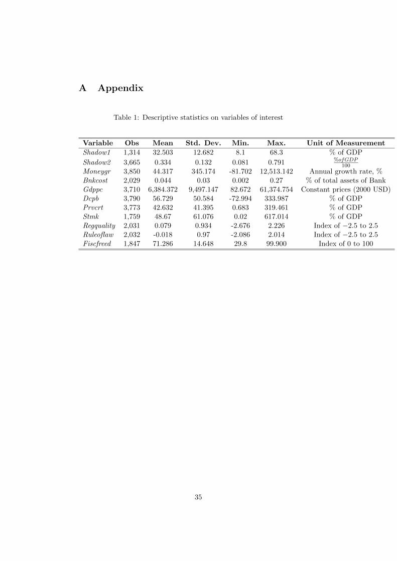
A Appendix

Table 1: Descriptive statistics on variables of interest

Variable Obs Mean Std. Dev. Min. Max. Unit of Measurement

Shadow1 1,314 32.503 12.682 8.1 68.3 % of GDP

Shadow2 3,665 0.334 0.132 0.081 0.791 %ofGDP100

Moneygr 3,850 44.317 345.174 -81.702 12,513.142 Annual growth rate, %Bnkcost 2,029 0.044 0.03 0.002 0.27 % of total assets of BankGdppc 3,710 6,384.372 9,497.147 82.672 61,374.754 Constant prices (2000 USD)Dcpb 3,790 56.729 50.584 -72.994 333.987 % of GDPPrvcrt 3,773 42.632 41.395 0.683 319.461 % of GDPStmk 1,759 48.67 61.076 0.02 617.014 % of GDPRegquality 2,031 0.079 0.934 -2.676 2.226 Index of −2.5 to 2.5Ruleoflaw 2,032 -0.018 0.97 -2.086 2.014 Index of −2.5 to 2.5Fiscfreed 1,847 71.286 14.648 29.8 99.900 Index of 0 to 100

35

Tab

le2:

Cor

rela

tion

Tab

le

Vari

ab

les

log

shad

ow1

log

shad

ow2

mon

eygr

log

bn

kcos

tfi

nd

evfi

nd

ev2

inst

itlo

gin

stit

log

gdp

pc

log

cba

log

shad

ow1

1.0

00

log

shad

ow2

0.993

*1.0

00

mon

eygr

0.2

93*

0.279

*1.

000

log

bn

kcost

0.493

*0.5

04*

0.26

6*1.

000

fin

dev

-0.6

80*

-0.6

66*

-0.4

27*

-0.5

85*

1.00

0fi

nd

ev2

-0.6

18*

-0.6

10*

-0.3

40*

-0.5

48*

0.91

8*1.

000

inst

it-0

.727

*-0

.717

*-0

.331

*-0

.351

*0.

690*

0.673

*1.0

00

log

inst

it-0

.628*

-0.5

57*

-0.2

13*

-0.1

47*

0.45

0*0.

448*

0.8

37*

1.0

00

log

gd

pp

c-0

.704

*-0

.685

*-0

.254

*-0

.380

*0.

679*

0.655

*0.8

02*

0.6

22*

1.0

00

log

cba

0.285

*0.2

96*

0.10

0*0.

182*

-0.1

60*

-0.1

52*

-0.3

62*

-0.0

98*

-0.3

73*

1.0

00

1.

A*

indic

ate

sth

e5%

signifi

cance

level

.

36

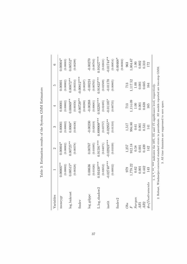
Tab

le3:

Est

imat

ion

resu

lts

ofth

eS

yst

emG

MM

Est

imat

ors

Vari

able

s1

23

45

6

mon

eygr

0.0

000

5**

0.00

004*

0.00

001

0.00

001

0.0

000

10.0

000

4*(0

.00002)

(0.0

0002)

(0.0

0002)

(0.0

0002)

(0.0

0002)

(0.0

0003)

log

bn

kcost

0.0

051

5*0.

0072

5**

0.00

68*

0.00

869*

*0.

008

72**

0.005

52*

(0.0

0328)

(0.0

0378)

(0.0

0436)

(0.0

0356)

(0.0

0354)

(0.0

0299)

fin

dev

-0.0

0729

**

-0.0

0812

***

(0.0

0280)

(0.0

0287)

log

gdp

pc

0.006

360.

0076

7-0

.002

30-0

.002

68-0

.002

24-0

.0027

0(0

.01026)

(0.0

1095)

(0.0

2019)

(0.0

0681)

(0.0

0765)

(0.0

0783)

L.l

ogsh

adow

20.9

343

9***

0.91

591*

**0.

8999

09**

*0.

9229

5***

0.918

23**

*0.

916

27**

*(0

.02652)

(0.0

4071)

(0.0

3757)

(0.0

2495)

(0.0

2509)

(0.0

2631)

inst

it-0

.0274

0***

-0.0

2923

***

-0.0

2955

**-0

.011

05*

-0.0

117

0-0

.017

44**

(0.0

0932)

(0.0

1039)

(0.0

1310)

(0.0

0735)

(0.0

0805)

(0.0

0854)

fin

dev

2-0

.0046

8*(0

.00302)

Obs

979

1,25

71,

517

713

713

963

F1,

778

.22

912.

1899

4.80

1,11

4.09

1,1

17.

52

1,004

.67

Sargan

0.62

0.58

0.61

1.00

1.00

1.0

0AR

10.

001

0.00

10.

001

0.00

10.0

01

0.002

AR

20.

442

0.43

90.

531

0.63

80.6

05

0.310

#ofInstruments

143

142

141

165

164

172

1.

A*,

**,

***

indic

ate

sth

e10%

,5%

and

1%

signifi

cance

level

,re

spec

tivel

y.

2.

Robust

,W

indm

eije

r-co

rrec

ted

standard

erro

rsin

pare

nth

esis

.A

llm

odel

sre

port

edare

two-s

tep

GM

M.

3.

All

tim

edum

mie

sare

suppre

ssed

tosa

ve

space

.

37

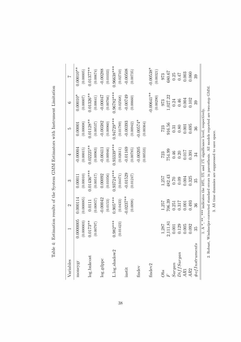
Tab

le4:

Est

imat

ion

resu

lts

ofth

eS

yst

emG

MM

Est

imat

ors

wit

hIn

stru

men

tL

imit

atio

n

Var

iab

les

12

34

56

7

mon

eygr

0.000

0005

0.0

0011

40.

0001

1-0

.000

040.

0000

10.0

001

0*0.

000

10**

(0.0

00003)

(0.0

00085)

(0.0

0010)

(0.0

0015)

(0.0

0008)

(0.0

0007)

(0.0

0005)

log

bn

kcos

t0.0

173

**0.

0111

0.01

436*

**0.

0222

5**

0.01

128*

*0.

013

26**

0.013

77**

(0.0

0797)

(0.0

0857)

(0.0

0517)

(0.0

0963)

(0.0

0537)

(0.0

0641)

(0.0

0674)

log

gd

pp

c-0

.000

420.

0009

2-0

.004

11-0

.0038

2-0

.0004

7-0

.002

88(0

.0153)

(0.0

1056)

(0.0

0946)

(0.0

0960)

(0.0

0766)

(0.0

1033)

L.l

og

shad

ow2

0.982

***

0.9

05**

*0.

9372

4***

0.93

339*

**0.

9472

9***

0.9

678

2***

0.9

663

8***

(0.0

1423)

(0.0

433)

(0.0

4471)

(0.0

2611)

(0.0

1789)

(0.0

2568)

(0.0

2710)

inst

it-0

.023

7**

-0.0

1529

-0.0

1169

-0.0

039

3-0

.007

49-0

.005

08(0

.0098)

(0.0

1247)

(0.0

0785)

(0.0

0942)

(0.0

0660)

(0.0

0735)

fin

dev

-0.0

0205

-0.0

0574

*(0

.00533)

(0.0

0364)

fin

dev

2-0

.0064

1**

-0.0

053

8*(0

.00290)

(0.0

0321)

Obs

1,287

1,25

71,

257

723

723

973

973

F2,

111

.81

706

.39

482.

4375

4.99

916.5

61,0

27.

22

680.

67

Sargan

0.001

0.25

10.

700.

460.

31

0.24

0.25

DiffSargan

0.129

0.31

70.

090.

200.

80

0.46

0.47

AR

10.

005

0.00

10.

004

0.01

70.

001

0.004

0.003

AR

20.

092

0.49

30.

325

0.39

10.

695

0.102

0.060

#ofInstruments

3536

3534

36

3939

1.

A*,

**,

***

indic

ate

sth

e10%

,5%

and

1%

signifi

cance

level

,re

spec

tivel

y.

2.

Robust

,W

indm

eije

r-co

rrec

ted

standard

erro

rsin

pare

nth

esis

.A

llm

odel

sre

port

edare

two-s

tep

GM

M.

3.

All

tim

edum

mie

sare

suppre

ssed

tosa

ve

space

.

38

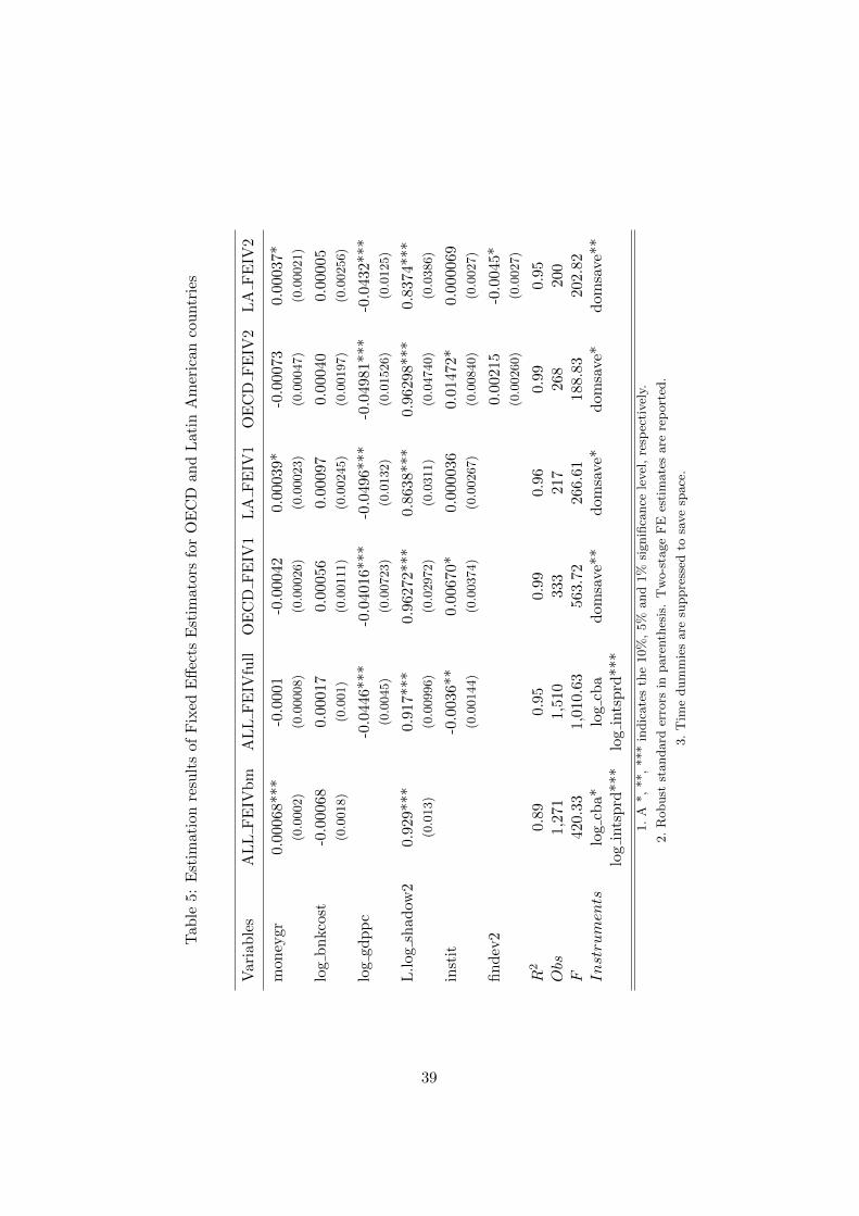
Tab

le5:

Est

imat

ion

resu

lts

ofF

ixed

Eff

ects

Est

imat

ors

for

OE

CD

and

Lati

nA

mer

ican

cou

ntr

ies

Vari

able

sA

LL

FE

IVb

mA

LL

FE

IVfu

llO

EC

DF

EIV

1L

AF

EIV

1O

EC

DF

EIV

2L

AF

EIV

2

mon

eygr

0.0

0068

***

-0.0

001

-0.0

0042

0.00

039*

-0.0

007

30.0

003

7*(0

.0002)

(0.0

0008)

(0.0

0026)

(0.0

0023)

(0.0

0047)

(0.0

0021)

log

bn

kcos

t-0

.000

680.

0001

70.

0005

60.

0009

70.0

004

00.

000

05(0

.0018)

(0.0

01)

(0.0

0111)

(0.0

0245)

(0.0

0197)

(0.0

0256)

log

gd

pp

c-0

.044

6***

-0.0

4016

***

-0.0

496*

**

-0.0

498

1***

-0.0

432*

**(0

.0045)

(0.0

0723)

(0.0

132)

(0.0

1526)

(0.0

125)

L.l

ogsh

adow

20.9

29*

**0.

917*

**0.

9627

2***

0.86

38***

0.9

629

8***

0.8

374

***

(0.0

13)

(0.0

0996)

(0.0

2972)

(0.0

311)

(0.0

4740)

(0.0

386)

inst

it-0

.003

6**

0.00

670*

0.00

0036

0.0

147

2*0.0

000

69(0

.00144)

(0.0

0374)

(0.0

0267)

(0.0

0840)

(0.0

027)

fin

dev

20.

002

15-0

.0045

*(0

.00260)

(0.0

027)

R2

0.89

0.95

0.99

0.96

0.9

90.9

5Obs

1,2

71

1,51

033

321

7268

200

F42

0.33

1,01

0.63

563.

7226

6.61

188

.83

202.

82

Instruments

log

cba*

log

cba

dom

save*

*d

omsa

ve*

dom

save

*d

omsa

ve*

*lo

gin

tsp

rd**

*lo

gin

tsp

rd**

*

1.

A*,

**,

***

indic

ate

sth

e10%

,5%

and

1%

signifi

cance

level

,re

spec

tivel

y.

2.

Robust

standard

erro

rsin

pare

nth

esis

.T

wo-s

tage

FE

esti

mate

sare

rep

ort

ed.

3.

Tim

edum

mie

sare

suppre

ssed

tosa

ve

space

.

39

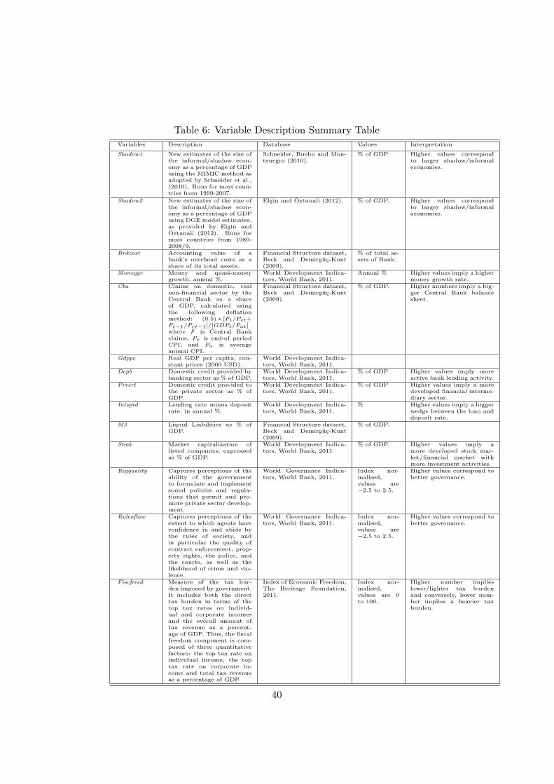
Table 6: Variable Description Summary Table

Variables Description Database Values Interpretation

Shadow1 New estimates of the size ofthe informal/shadow econ-omy as a percentage of GDPusing the MIMIC method asadopted by Schneider et al.,(2010). Runs for most coun-tries from 1999-2007.

Schneider, Buehn and Mon-tenegro (2010).

% of GDP Higher values correspondto larger shadow/informaleconomies.

Shadow2 New estimates of the size ofthe informal/shadow econ-omy as a percentage of GDPusing DGE model estimates,as provided by Elgin andOztunali (2012). Runs formost countries from 1980-2008/9.

Elgin and Oztunali (2012). % of GDP. Higher values correspondto larger shadow/informaleconomies.

Bnkcost Accounting value of abank’s overhead costs as ashare of its total assets.

Financial Structure dataset,Beck and Demirguc-Kunt(2009).

% of total as-sets of Bank.

Moneygr Money and quasi-moneygrowth, annual %.

World Development Indica-tors, World Bank, 2011.

Annual % Higher values imply a highermoney growth rate.

Cba Claims on domestic, realnon-financial sector by theCentral Bank as a shareof GDP, calculated usingthe following deflationmethod: (0.5) ∗ [Ft/Pet+Ft−1/Pet−1]/[GDPt/Pat]where F is Central Bankclaims, Pe is end-of periodCPI, and Pa is averageannual CPI.

Financial Structure dataset,Beck and Demirguc-Kunt(2009).

% of GDP. Higher numbers imply a big-ger Central Bank balancesheet.

Gdppc Real GDP per capita, con-stant prices (2000 USD).

World Development Indica-tors, World Bank, 2011.

Dcpb Domestic credit provided bybanking sector as % of GDP.

World Development Indica-tors, World Bank, 2011.

% of GDP Higher values imply moreactive bank lending activity.

Prvcrt Domestic credit provided tothe private sector as % ofGDP.

World Development Indica-tors, World Bank, 2011.

% of GDP Higher values imply a moredeveloped financial interme-diary sector.

Intsprd Lending rate minus depositrate, in annual %.

World Development Indica-tors, World Bank, 2011.

% Higher values imply a biggerwedge between the loan anddeposit rate.

M3 Liquid Liabilities as % ofGDP.

Financial Structure dataset,Beck and Demirguc-Kunt(2009).

% of GDP.

Stmk Market capitalization oflisted companies, expressedas % of GDP.

World Development Indica-tors, World Bank, 2011.

% of GDP. Higher values imply amore developed stock mar-ket/financial market withmore investment activities.

Regquality Captures perceptions of theability of the governmentto formulate and implementsound policies and regula-tions that permit and pro-mote private sector develop-ment.

World Governance Indica-tors, World Bank, 2011.

Index nor-malised,values are−2.5 to 2.5.

Higher values correspond tobetter governance.

Ruleoflaw Captures perceptions of theextent to which agents haveconfidence in and abide bythe rules of society, andin particular the quality ofcontract enforcement, prop-erty rights, the police, andthe courts, as well as thelikelihood of crime and vio-lence.

World Governance Indica-tors, World Bank, 2011.

Index nor-malised,values are−2.5 to 2.5.

Higher values correspond tobetter governance.

Fiscfreed Measure of the tax bur-den imposed by government.It includes both the directtax burden in terms of thetop tax rates on individ-ual and corporate incomesand the overall amount oftax revenue as a percent-age of GDP. Thus, the fiscalfreedom component is com-posed of three quantitativefactors: the top tax rate onindividual income, the toptax rate on corporate in-come and total tax revenueas a percentage of GDP.

Index of Economic Freedom,The Heritage Foundation,2011.

Index nor-malised,values are 0to 100.

Higher number implieslower/lighter tax burdenand conversely, lower num-ber implies a heavier taxburden.

40