tatsuki koyama, phd

SELECTED TOPICS IN PHASE II AND IIICLINICAL TRIALS

Tatsuki Koyama, PhDDepartment of Biostatistics, Vanderbilt University Medical Center

[email protected]

Osaka City University, Biostatistics.November 10 ∼ 18, 2021

Last updated: 2021-11-08 13:10R version: 4.1.1

Copyright 2021. T Koyama. All Rights Reserved.

Contents

1 Overview 21.1 Observational Study: CEASAR . . . . . . . . . . . . . . . . . . . . . . . . . . . . . . . 21.2 Experiment . . . . . . . . . . . . . . . . . . . . . . . . . . . . . . . . . . . . . . . . . . 5

1.2.1 Example: PIVOT . . . . . . . . . . . . . . . . . . . . . . . . . . . . . . . . . . . 6

2 Multiplicity in Clinical Trials -FDA’s Guidance- 82.1 Background . . . . . . . . . . . . . . . . . . . . . . . . . . . . . . . . . . . . . . . . . . 82.2 Statistical methods . . . . . . . . . . . . . . . . . . . . . . . . . . . . . . . . . . . . . . 112.3 Graphical approach . . . . . . . . . . . . . . . . . . . . . . . . . . . . . . . . . . . . . 14

3 Randomization 193.1 Example: Polio vaccine trial (1954) . . . . . . . . . . . . . . . . . . . . . . . . . . . . . 193.2 Introduction . . . . . . . . . . . . . . . . . . . . . . . . . . . . . . . . . . . . . . . . . . 203.3 Simple randomization . . . . . . . . . . . . . . . . . . . . . . . . . . . . . . . . . . . . 213.4 Imbalance in treatment allocation . . . . . . . . . . . . . . . . . . . . . . . . . . . . . . 21

3.4.1 Block randomization . . . . . . . . . . . . . . . . . . . . . . . . . . . . . . . . . 213.4.2 Biased coin and urn model . . . . . . . . . . . . . . . . . . . . . . . . . . . . . 24

3.5 Imbalance in baseline patient characteristics . . . . . . . . . . . . . . . . . . . . . . . 253.5.1 Stratified randomization . . . . . . . . . . . . . . . . . . . . . . . . . . . . . . . 253.5.2 Adaptive and minimization randomization . . . . . . . . . . . . . . . . . . . . . 26

3.6 Response adaptive randomization . . . . . . . . . . . . . . . . . . . . . . . . . . . . . 273.6.1 Example: ECMO . . . . . . . . . . . . . . . . . . . . . . . . . . . . . . . . . . . 27

3.7 Nonbipartite matching in clinical trials . . . . . . . . . . . . . . . . . . . . . . . . . . . 293.7.1 Example . . . . . . . . . . . . . . . . . . . . . . . . . . . . . . . . . . . . . . . . 29

4 Superiority, Non-inferiority, and equivalence 354.1 Superiority and non-inferiority . . . . . . . . . . . . . . . . . . . . . . . . . . . . . . . . 354.2 Equivalence . . . . . . . . . . . . . . . . . . . . . . . . . . . . . . . . . . . . . . . . . . 38

5 Phase II Oncology Clinical Trials 405.1 Introduction . . . . . . . . . . . . . . . . . . . . . . . . . . . . . . . . . . . . . . . . . . 405.2 Phase II trials in oncology . . . . . . . . . . . . . . . . . . . . . . . . . . . . . . . . . . 415.3 Classical (old) two-stage designs . . . . . . . . . . . . . . . . . . . . . . . . . . . . . . 42

5.3.1 Gehan’s design . . . . . . . . . . . . . . . . . . . . . . . . . . . . . . . . . . . . 425.3.2 Fleming’s design . . . . . . . . . . . . . . . . . . . . . . . . . . . . . . . . . . . 42

5.4 Simon’s design . . . . . . . . . . . . . . . . . . . . . . . . . . . . . . . . . . . . . . . . 435.4.1 Conditional power . . . . . . . . . . . . . . . . . . . . . . . . . . . . . . . . . . 435.4.2 Computing design characteristics . . . . . . . . . . . . . . . . . . . . . . . . . . 445.4.3 Something in between . . . . . . . . . . . . . . . . . . . . . . . . . . . . . . . . 48

5.5 Data analysis following a two-stage design in phase II clinical trials . . . . . . . . . . . 495.5.1 p-value . . . . . . . . . . . . . . . . . . . . . . . . . . . . . . . . . . . . . . . . 495.5.2 Point estimate . . . . . . . . . . . . . . . . . . . . . . . . . . . . . . . . . . . . 52

6 Factorial design 576.1 Introduction . . . . . . . . . . . . . . . . . . . . . . . . . . . . . . . . . . . . . . . . . . 576.2 Notation and assumptions . . . . . . . . . . . . . . . . . . . . . . . . . . . . . . . . . . 586.3 Test for the interaction effect . . . . . . . . . . . . . . . . . . . . . . . . . . . . . . . . . 596.4 Treatemnt effect . . . . . . . . . . . . . . . . . . . . . . . . . . . . . . . . . . . . . . . 60

6.4.1 γ 6= 0 . . . . . . . . . . . . . . . . . . . . . . . . . . . . . . . . . . . . . . . . . . 606.4.2 γ = 0 . . . . . . . . . . . . . . . . . . . . . . . . . . . . . . . . . . . . . . . . . . 61

6.5 Examples . . . . . . . . . . . . . . . . . . . . . . . . . . . . . . . . . . . . . . . . . . . 616.5.1 Example: the Physician’s Health Study I (1989) . . . . . . . . . . . . . . . . . . 63

6.6 Treatment interactions . . . . . . . . . . . . . . . . . . . . . . . . . . . . . . . . . . . . 64

7 Crossover design 667.1 Some characteristics of crossover design . . . . . . . . . . . . . . . . . . . . . . . . . 677.2 Analysis of 2×2 crossover design . . . . . . . . . . . . . . . . . . . . . . . . . . . . . 68

7.2.1 Variance of β . . . . . . . . . . . . . . . . . . . . . . . . . . . . . . . . . . . . . 727.3 Examples . . . . . . . . . . . . . . . . . . . . . . . . . . . . . . . . . . . . . . . . . . . 74

7.3.1 From clinicalTrials.gov . . . . . . . . . . . . . . . . . . . . . . . . . . . . . . . . 747.4 Examples . . . . . . . . . . . . . . . . . . . . . . . . . . . . . . . . . . . . . . . . . . . 75

7.4.1 Hills and Armitage . . . . . . . . . . . . . . . . . . . . . . . . . . . . . . . . . . 757.5 A two-period crossover design for the comparison of two active treatments and placebo 787.6 Latin squares . . . . . . . . . . . . . . . . . . . . . . . . . . . . . . . . . . . . . . . . . 807.7 Optimal designs . . . . . . . . . . . . . . . . . . . . . . . . . . . . . . . . . . . . . . . 80

8 Group sequential design 838.1 Introduction . . . . . . . . . . . . . . . . . . . . . . . . . . . . . . . . . . . . . . . . . . 838.2 Example . . . . . . . . . . . . . . . . . . . . . . . . . . . . . . . . . . . . . . . . . . . . 848.3 General applications . . . . . . . . . . . . . . . . . . . . . . . . . . . . . . . . . . . . . 88

Clinical Trials 3 Tatsuki Koyama, PhD

8.3.1 Beta blocker heart attack trial . . . . . . . . . . . . . . . . . . . . . . . . . . . . 908.3.2 non-Hodgkin’s lymphoma . . . . . . . . . . . . . . . . . . . . . . . . . . . . . . 91

8.4 Alpha-spending . . . . . . . . . . . . . . . . . . . . . . . . . . . . . . . . . . . . . . . . 928.5 One-sided test . . . . . . . . . . . . . . . . . . . . . . . . . . . . . . . . . . . . . . . . 948.6 Repeated confidence intervals . . . . . . . . . . . . . . . . . . . . . . . . . . . . . . . 958.7 p-values . . . . . . . . . . . . . . . . . . . . . . . . . . . . . . . . . . . . . . . . . . . . 97

9 General Adaptive Designs 999.1 Introduction . . . . . . . . . . . . . . . . . . . . . . . . . . . . . . . . . . . . . . . . . . 999.2 Background . . . . . . . . . . . . . . . . . . . . . . . . . . . . . . . . . . . . . . . . . . 1009.3 Conditional power . . . . . . . . . . . . . . . . . . . . . . . . . . . . . . . . . . . . . . 1019.4 Two-stage design -without all the math- . . . . . . . . . . . . . . . . . . . . . . . . . . 1039.5 Conditional power functions . . . . . . . . . . . . . . . . . . . . . . . . . . . . . . . . . 1059.6 Example . . . . . . . . . . . . . . . . . . . . . . . . . . . . . . . . . . . . . . . . . . . . 1059.7 Unspecified designs . . . . . . . . . . . . . . . . . . . . . . . . . . . . . . . . . . . . . 1129.8 Ordering of sample space . . . . . . . . . . . . . . . . . . . . . . . . . . . . . . . . . . 1149.9 Predictive power . . . . . . . . . . . . . . . . . . . . . . . . . . . . . . . . . . . . . . . 117

Chapter 1

Overview

1.1 Observational Study: CEASAR

Prostate cancer is the second leading cause of cancer death among American men behind lungcancer. The common treatment choices for localized disease are surgery, radiation, and observation(active surveillance). For localized prostate cancer, 5-year survival is nearly 100%, and in compar-ative effectiveness studies, patient-reported disease-specific functional outcomes are often used asthe primary endpoint. The Comparative Effectiveness Analysis of Surgery and Radiation (CEASAR)study1 assessed patient-reported functional outcomes and health-related quality of life at 3 yearsafter treatment.Suppose we are interested in comparing the Sexual Functional Score (QOL) after 3 years fromtreatment.

groupSum(d$Epic36, d$Treatment, Combined = FALSE)

N Min Q1 Med Q3 Max Mean SD SESurgery 1222 0 10.00 33.3 70 100 41.0 33.4 0.96Radiation 691 0 6.67 38.3 70 100 40.4 33.5 1.27

with(d, t.test(Epic36 ~ Treatment))

Welch Two Sample t-test

data: Epic36 by Treatment

1Barocas et al., “Association between radiation therapy, surgery, or observation for localized prostate cancer andpatient-reported outcomes after 3 years” JAMA. 2017. 317(11):1126-1140.


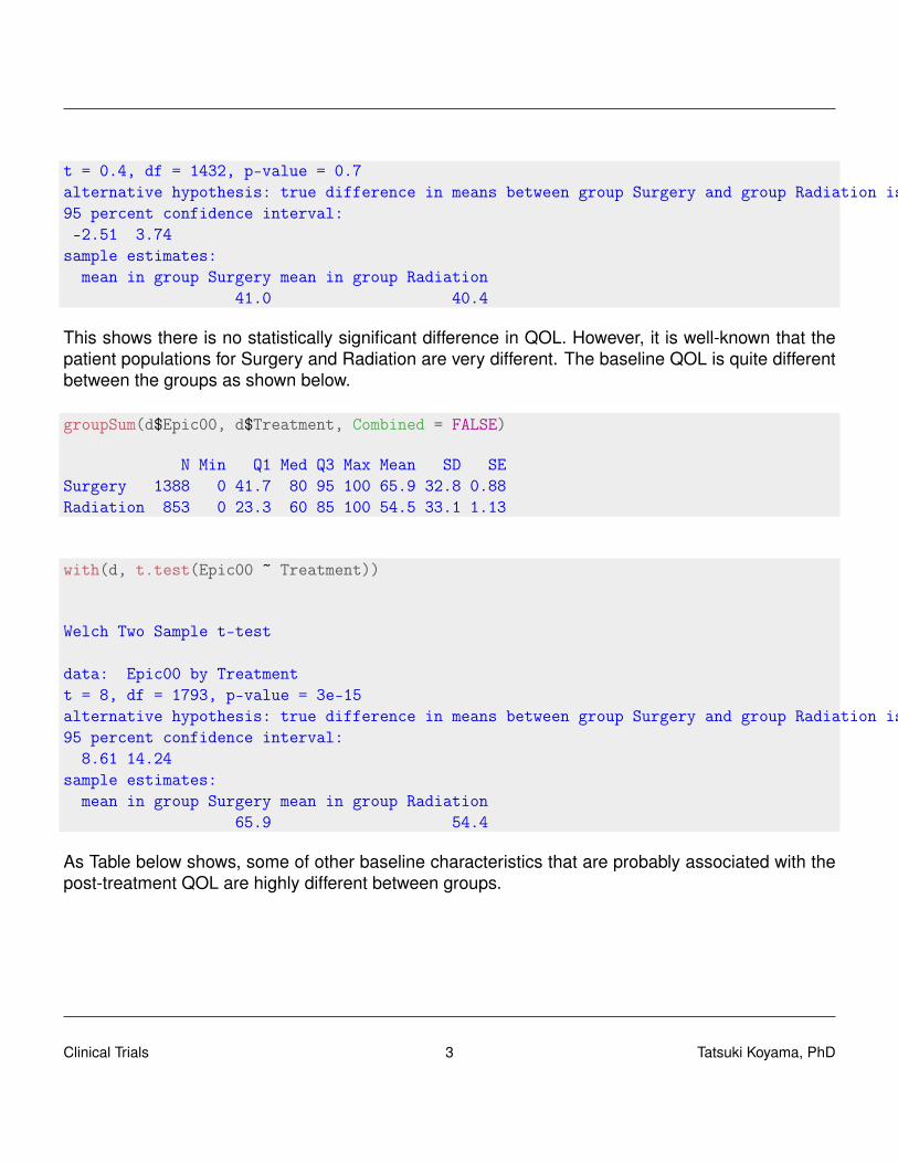
t = 0.4, df = 1432, p-value = 0.7alternative hypothesis: true difference in means between group Surgery and group Radiation is not equal to 095 percent confidence interval:-2.51 3.74

sample estimates:mean in group Surgery mean in group Radiation

41.0 40.4

This shows there is no statistically significant difference in QOL. However, it is well-known that thepatient populations for Surgery and Radiation are very different. The baseline QOL is quite differentbetween the groups as shown below.

groupSum(d$Epic00, d$Treatment, Combined = FALSE)

N Min Q1 Med Q3 Max Mean SD SESurgery 1388 0 41.7 80 95 100 65.9 32.8 0.88Radiation 853 0 23.3 60 85 100 54.5 33.1 1.13

with(d, t.test(Epic00 ~ Treatment))

Welch Two Sample t-test

data: Epic00 by Treatmentt = 8, df = 1793, p-value = 3e-15alternative hypothesis: true difference in means between group Surgery and group Radiation is not equal to 095 percent confidence interval:

8.61 14.24sample estimates:

mean in group Surgery mean in group Radiation65.9 54.4

As Table below shows, some of other baseline characteristics that are probably associated with thepost-treatment QOL are highly different between groups.


Table 1.1: CEASAR baseline characteristics

N Surgery Radiation Test StatisticN = 1455 N = 908

Age at diagnosis 2363 57 62 66 63 68 73 F1,2361=417, P<0.0011

Race : White 2363 75% (1088) 73% ( 662) χ23 =10.4, P=0.0162

Black 12% ( 175) 16% ( 148)

Hispanic 8% ( 113) 6% ( 57)

Others 5% ( 79) 5% ( 41)

TIBI cat : 0-2 2279 33% (468) 20% (175) χ23 =98.6, P<0.0012

3-5 55% (766) 55% (478)

6-8 10% (147) 19% (169)

9-15 2% ( 22) 6% ( 54)

DAmico Prostate Cancer Risk : Low Risk 2357 41% (597) 34% (307) χ22 =17, P<0.0012

Intermediate Risk 42% (613) 44% (395)

High Risk 17% (243) 22% (202)

PSA at diagnosis, corrected 2363 4.2 5.1 6.9 4.5 5.9 8.5 F1,2361=49, P<0.0011

Marital Status : Not married 2262 17% ( 234) 25% ( 215) χ21 =21.2, P<0.0012

Married 83% (1159) 75% ( 654)

Education : Less than high school 2266 9% (120) 13% (111) χ24 =15, P=0.0052

High school graduate 21% (294) 21% (186)

Some college 22% (306) 24% (208)

College graduate 24% (336) 21% (185)

Graduate/professional school 24% (340) 21% (180)

Income : Less than $30,000 2132 17% (228) 28% (224) χ23 =67.7, P<0.0012

$30,001 - $50,000 17% (223) 23% (187)

$50,001 - $100,000 33% (439) 29% (238)

More than $100,000 33% (432) 20% (161)

SF36 Physical Score 2287 85 100 100 75 90 100 F1,2285=87.4, P<0.0011

EPIC Sexual Function -Baseline 2241 41.7 80.0 95.0 23.3 60.0 85.0 F1,2239=76.9, P<0.0011

EPIC Sexual Function -3 years 1913 10.00 33.33 70.00 6.67 38.33 70.00 F1,1911=0.4, P=0.5281

a b c represent the lower quartile a, the median b, and the upper quartile c for continuous variables.N is the number of non–missing values. Numbers after percents are frequencies. Tests used:1Wilcoxon test; 2Pearson test


In general, establishing a cause-and-effect association from an observational study is difficult dueto confounders.

Confounder A prognostic factor that is associated with both response (e.g., Quality of Life) andexplanatory variable (e.g., treatment choice).

We can analyze the data with a method that accounts for the baseline difference in the treatmentgroups.

QOL ∼ Treatment × (Baseline QOL + Age + Race + TIBI + Risk + PSA)

How about comorbidities? sex? smoking?Many statistical methods exist to establish causal relationships from an observation study such aspropensity scores and instrumental variables.

Can observational studies establish a cause-and-effect association?

Philip Morris Internationalhttps://www.pmi.com/our-business/about-us/our-views/health-effects-of-smoking-tobacco

• “Cigarette smoking causes serious disease and is addictive.”

• “All cigarettes are harmful and addictive.”

• “Public health authorities have concluded that secondhand smoke causes diseases, includinglung cancer and heart disease, ...”

JThttps://www.jti.co.jp/tobacco/responsibilities/guidelines/responsibility/index.htmlhttps://www.jti.com/about-us/our-business/our-six-core-principles

• “Smoking is a cause of serious diseases including lung cancer, coronary heart disease, em-physema and chronic bronchitis.”

• “All relevant risk factors need to be taken into consideration when investigating the cause orcauses of a disease in any smoker.”

1.2 Experiment

Observational study A study design in which the investigator does not control the assignment oftreatment of individual study subjects (Piantadosi2)

2Clinical Trials: A Methodologic Perspective


Experiment A study in which the investigator makes a series of observations under controlled/arrangedconditions. In particular, the investigator controls the treatment applied to the subjects by de-sign. (Piantadosi)

Clinical trial A prospective study comparing the effect and value of an intervention against acontrol in human subjects (Friedman3)

Advantages of observational studies include:

• Lower cost.

• Greater timeliness.

• A broad range of patients.

• Greater application where experiments would be impossible or unethical.

The advantage of clinical trials is that they can establish a cause-and-effect association.

1.2.1 Example: PIVOT

In Prostate Cancer Intervention Versus Observation Trial4 (PIVOT), prostate cancer patients whowere good candidates for radical prostatectomy were enrolled from 1994 to 2002. The last obser-vation was made in 2010. The results were presented at American Urological Association AnnualMeeting in May, 2011. The inclusion criteria for the study were:

• 75 years or younger.

• Localized disease.

• PSA ≤ 50mg/mg.

• Diagnosed with 12 months.

• Radical prostatectomy candidate.

With the all-cause mortality as the primary endpoint, the primary objective was to answer the follow-ing question:

Among men with clinically localized prostate cancer detected during the early PSA era,does the intent to treat with radical prostatectomy reduce all-cause & prostate cancermortality compared to observation?

3Fundamentals of Clinical Trials4Wilt et al. (PIVOT Study Group). “Radical prostatectomy versus observation for localized prostate cancer”. N Engl J

Med. 2012. 367(3):203–213.


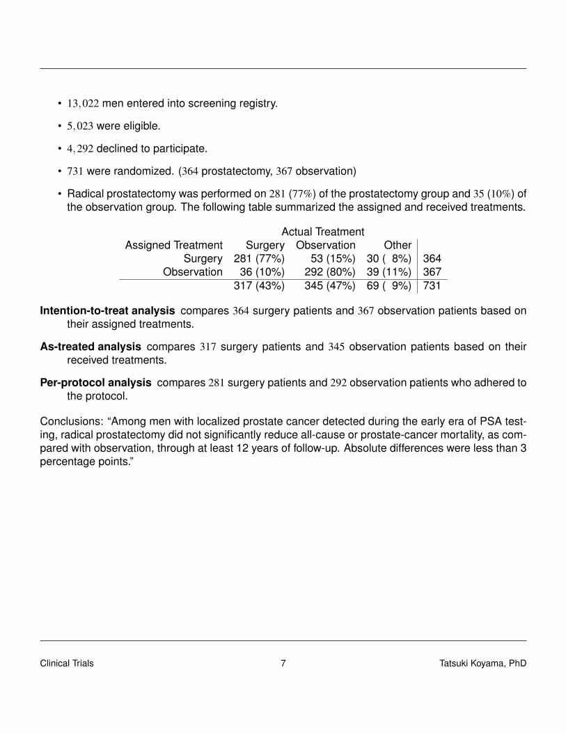
• 13,022 men entered into screening registry.

• 5,023 were eligible.

• 4,292 declined to participate.

• 731 were randomized. (364 prostatectomy, 367 observation)

• Radical prostatectomy was performed on 281 (77%) of the prostatectomy group and 35 (10%) ofthe observation group. The following table summarized the assigned and received treatments.

Actual TreatmentAssigned Treatment Surgery Observation Other

Surgery 281 (77%) 53 (15%) 30 ( 8%) 364Observation 36 (10%) 292 (80%) 39 (11%) 367

317 (43%) 345 (47%) 69 ( 9%) 731

Intention-to-treat analysis compares 364 surgery patients and 367 observation patients based ontheir assigned treatments.

As-treated analysis compares 317 surgery patients and 345 observation patients based on theirreceived treatments.

Per-protocol analysis compares 281 surgery patients and 292 observation patients who adhered tothe protocol.

Conclusions: “Among men with localized prostate cancer detected during the early era of PSA test-ing, radical prostatectomy did not significantly reduce all-cause or prostate-cancer mortality, as com-pared with observation, through at least 12 years of follow-up. Absolute differences were less than 3percentage points.”


Chapter 2

Multiplicity in Clinical Trials -FDA’sGuidance-

2.1 Background

The problem When K hypothesis tests are conducted with type I error rate of α, the overall type Ierror rate becomes higher than α.The overall type I error rate = P[At least one type I error] = Family-wise error.

Suppose there are 8 hypothesis tests, and each is conducted at 5% level. Then

P[At least one type I error] = 1−P[no type I error]

= 1− (1−0.05)8

= 0.337

And to control the family-wise type I error rate at 5%, each test must be conducted at α = 0.00639because

1− (1−0.00639)8 = 0.05

Recent development

2016.12 EMA: Guideline on multiplicity issues in clinical trials

2017.1 FDA: Draft guidance. Multiple endpoints in clinical trials

2017.8 Stat in Med: A Dmitrienko and RB D’Agostino. “Editorial: Multiplicity issues in clinical trials”

2018.1 Journal of Biopharm Stat: Special issue on multiplicity issues in clinical trials


2018.5 NEJM: A Dmitrienko and RB D’Agostino. “Multiplicity considerations in clinical trials”

Guidelines

• EMA: Guideline on multiplicity issues in clinical trials (Draft)

– 15 pages

– Draft published on 12/15/2016

– Replaces “Points to consider on multiplicity issues in clinical trials” (Adopted 2002)

• FDA: Multiple endpoints in clinical trials: Guidance for industry

– 50 pages

– Draft published in January 2017

– Details on statistical methods in addition to general principles

Prespecification is necessary.“An important principle for controlling multiplicity is to prospectively specify all planned endpoints,time points, analysis populations, and analyses.”

Multiplicity topics / sources of multiplicity

• Multiple endpoints

– Primary endpoint family

– Secondary endpoint family

– (Exploratory endpoints)

– Co-primary endpoints

– Composite endpoints/multi-component

• Multiple looks

– Interim analyses (“outside the scope” (FDA))

• Multiple analyses

– Subgroup analyses

– Multiple analyses methods


• Superiority/Non-inferiority (FDA)

• Safety variables (EMA)

• Multiple treatment arms (EMA)

• Dose-response studies (EMA)

• Estimation (EMA)

Endpoints

• Primary endpoints“Success on any one alone could be considered sufficient to demonstrate the drug’s effective-ness”

• Secondary endpointsProvide additional evidence of efficacy.

• Exploratory endpoints“All other endpoints” (Is adjustment necessary?)“endpoints that are thought to be less likely to show an effect but are included to explore newhypotheses”

Endpoints are frequently ordered by

– clinical importance (Mortality as primary)

– the likelihood of demonstrating an effect (PFS as primary, OS as secondary)

Composite endpointCombine clinical outcomes into a single variable.

• Cardiovascular death OR heart attack OR stroke. (coronary artery disease)

• MAKE 30 (Major Adverse Kidney Events: impaired renal function OR hemodialysis OR death(AKI)

“Analyses of the components of the composite endpoint are important and can influence interpreta-tion of the overall study results.”

Co-primary endpointsDemonstration of treatment effects on more than one endpoint is necessary to conclude efficacy.FDA requires each test be done at 5% level.

Relaxation of alpha ... would undermine the assurance of an effect on each diseaseaspect considered essential to showing that the drug is effective.


α = 0.22 (0.222 ≈ 0.05) if independent.Type II error rate inflation may be severe. (0.052 = 0.0025)

• Co-endpoints are likely to be correlated, but the correlation is unknown.

• Contrast this to a group sequential design where the correlation of accumulated data can becomputed.Cov(Z j, Zk) =

√N j/Nk.

α1 = 0.030 and α2 = 0.030 for the Pocock boundary.

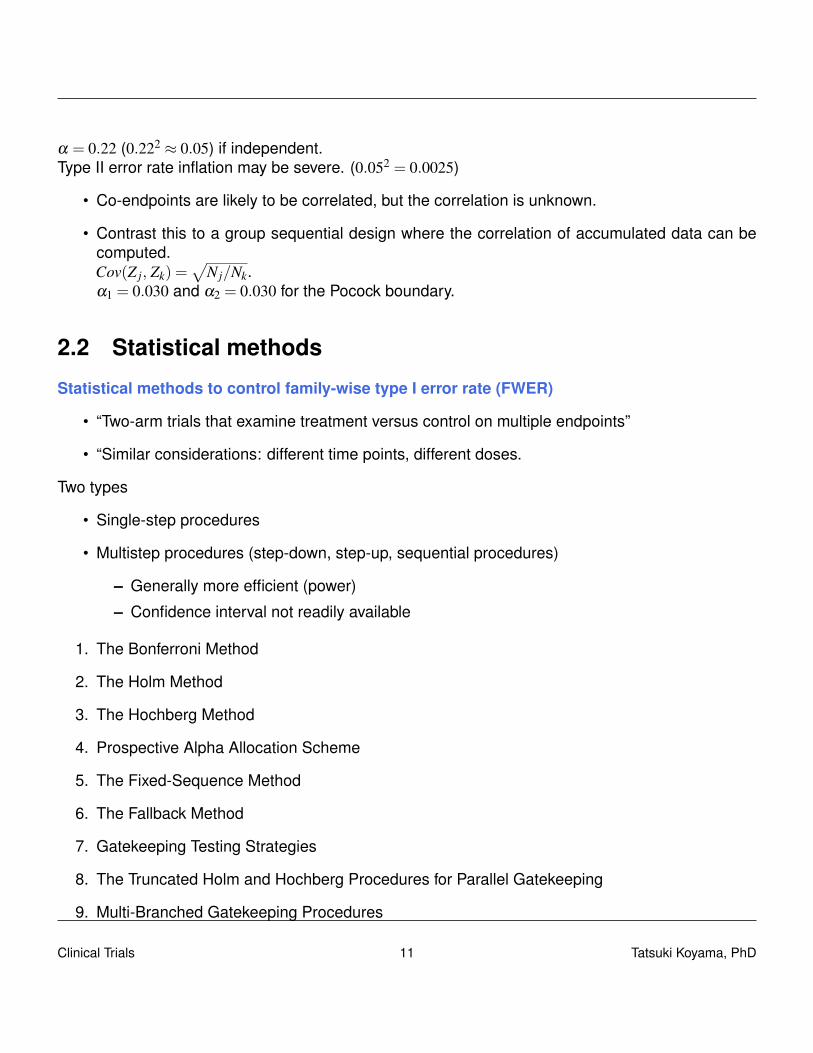
2.2 Statistical methods

Statistical methods to control family-wise type I error rate (FWER)

• “Two-arm trials that examine treatment versus control on multiple endpoints”

• “Similar considerations: different time points, different doses.

Two types

• Single-step procedures

• Multistep procedures (step-down, step-up, sequential procedures)

– Generally more efficient (power)

– Confidence interval not readily available

1. The Bonferroni Method

2. The Holm Method

3. The Hochberg Method

4. Prospective Alpha Allocation Scheme

5. The Fixed-Sequence Method

6. The Fallback Method

7. Gatekeeping Testing Strategies

8. The Truncated Holm and Hochberg Procedures for Parallel Gatekeeping

9. Multi-Branched Gatekeeping Procedures


10. Resampling-Based, Multiple-Testing Procedures

Common Statistical Method

1. Bonferroni (Single step; assumption free)Each hypothesis test is conducted at α/K level. α/K ≈ the solution, a, to α = 1− (1−a)K.

2. Holm (Multi-step step down; assumption free)H1, · · · ,Hm is a family of m null hypotheses, and P1, · · · ,Pm are the corresponding P-values.The ordered P-values, P[i] are compared to α/(m+1− k), and let k be the smallest index suchthat P[i] > α/(m+1− i). Reject the null hypotheses H(1), · · · ,H(k−1).

Example:α = 0.05. p1 = 0.015, p2 = 0.03, p3 = 0.04, p4 = 0.01.

Bonferroni method:Each p-value is compared to α/4 = 0.013. Only H4 is rejected.

Holm method:p[1] = 0.01, p[2] = 0.015, p[3] = 0.03, p[4] = 0.04.The corresponding critical values are0.05/4 = 0.013, 0.05/3 = 0.017, 0.05/2 = 0.025, and 0.05.

3. Hochberg (Multi-step step up; Positive correlation)Similar to Holm but backwards. Start comparing the largest p-value to α and work the waydown to the smallest p-value. Reject all H0 once p[k] < α/(m+1− k).

4. Prospective Alpha Allocation Scheme (Single step; Positive correlation)

Similar to Bonferroni, but use α1, α2, · · · , αm such that

(1−α1)×·· ·× (1−αm) = (1−α).

Example: (1−0.00639)8 = 1−0.05

FDA on Hochberg:

· · · beyond the aforementioned cases where the Hochberg procedure is known to bevalid, its use is generally not recommended for the primary comparisons of confirmatoryclinical trials unless it can be shown that adequate control of Type I error rate is provided.

Sequential method

5. Fixed-Sequence MethodTests endpoints in a predefined order, all at α = 0.05, moving to the next endpoint only after asuccess on the previous endpoint.


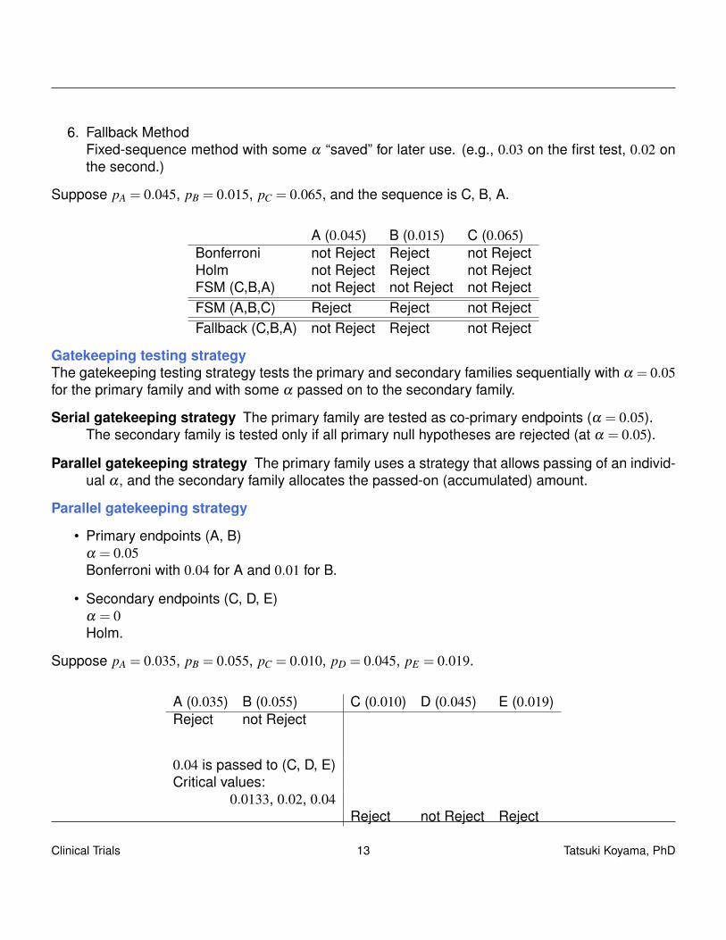
6. Fallback MethodFixed-sequence method with some α “saved” for later use. (e.g., 0.03 on the first test, 0.02 onthe second.)

Suppose pA = 0.045, pB = 0.015, pC = 0.065, and the sequence is C, B, A.

A (0.045) B (0.015) C (0.065)Bonferroni not Reject Reject not RejectHolm not Reject Reject not RejectFSM (C,B,A) not Reject not Reject not RejectFSM (A,B,C) Reject Reject not RejectFallback (C,B,A) not Reject Reject not Reject

Gatekeeping testing strategyThe gatekeeping testing strategy tests the primary and secondary families sequentially with α = 0.05for the primary family and with some α passed on to the secondary family.

Serial gatekeeping strategy The primary family are tested as co-primary endpoints (α = 0.05).The secondary family is tested only if all primary null hypotheses are rejected (at α = 0.05).

Parallel gatekeeping strategy The primary family uses a strategy that allows passing of an individ-ual α, and the secondary family allocates the passed-on (accumulated) amount.

Parallel gatekeeping strategy

• Primary endpoints (A, B)α = 0.05Bonferroni with 0.04 for A and 0.01 for B.

• Secondary endpoints (C, D, E)α = 0Holm.

Suppose pA = 0.035, pB = 0.055, pC = 0.010, pD = 0.045, pE = 0.019.

A (0.035) B (0.055) C (0.010) D (0.045) E (0.019)Reject not Reject

0.04 is passed to (C, D, E)Critical values:

0.0133, 0.02, 0.04Reject not Reject Reject


2.3 Graphical approach

Using gMCP package in R.

• K Rohmeyer, F Klinglmueller (2018). gMCP: Graph Based Multiple Test Procedures. R pack-age version 0.8-14.

• F Bretz, M Posch, EGlimm, FKlinglmueller, W Maurer, K Rohmeyer (2011), Graphical ap-proaches for multiple comparison procedures using weighted Bonferroni, Simes or parametrictests. Biometrical Journal 53(6), pages:894-913.

Bonferroni

H1

0.025

H2

0.025p1 = 0.04 p2 = 0.02

Holm

H1

0.025

H2

0.025

1

1

p1 = 0.04 p2 = 0.02

Holm procedure with 3 hypotheses


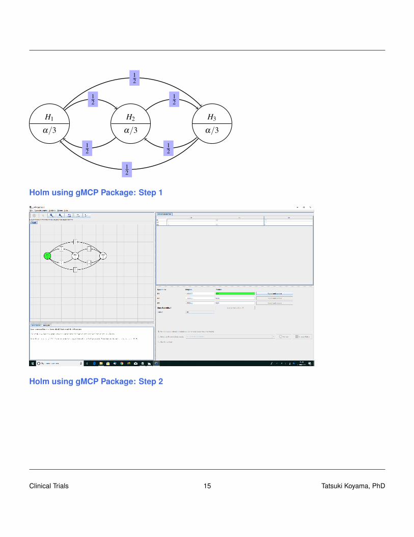
H1

α/3

H2

α/3

H3

α/3

12

12

12

12

12

12

Holm using gMCP Package: Step 1

Holm using gMCP Package: Step 2


Fixed sequence method

H1

α

H2

0

H3

01 1

Fall back method

H1

α/3

H2

α/3

H3

α/31 1

Improved fall back method

H1α/3

H2α/3

H3α/3

11

12

12


Improved fall back with gMCP package: Step 1




A Parallel gatekeeping procedure

H1

1/2

H2

1/2

H3

0

H4

0

12

12

12 1

2

1

1

Primary

Secondary


Chapter 3

Randomization

3.1 Example: Polio vaccine trial (1954)

In 1954, 1.8 million children participated in the largest clinical trial to date to assess the effectivenessof the vaccine developed by Jonas Salk in preventing paralysis or death from poliomyelitis.

• 1.8 million children in selected school districts throughout the US were involved in this placebo-controlled trial.

– Why was placebo necessary?

– 60,000 cases in 1952; about half of that in 1953.

• Randomized trial.

– 750,000 children participated.

– They required parents’ consent.

– Half of the children with consent were randomized into the vaccine group.

• NFIP design.

– The National Foundation for Infantile Paralysis (NFIP) conducted a study in which all 2ndgraders with consent received the vaccine with 1st and 3rd graders acting as control.

– 1,125,000 children participated.

– The control children did not require consent.Systematic difference between groups.

– No blinding.

– Polio is a contagious disease!


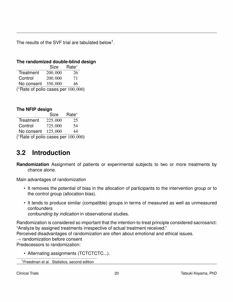
The results of the SVF trial are tabulated below1.

The randomized double-blind designSize Rate∗

Treatment 200,000 26Control 200,000 71No consent 350,000 46

(∗Rate of polio cases per 100,000)

The NFIP designSize Rate∗

Treatment 225,000 25Control 725,000 54No consent 125,000 44

(∗Rate of polio cases per 100,000)

3.2 Introduction

Randomization Assignment of patients or experimental subjects to two or more treatments bychance alone.

Main advantages of randomization

• It removes the potential of bias in the allocation of participants to the intervention group or tothe control group (allocation bias).

• It tends to produce similar (compatible) groups in terms of measured as well as unmeasuredconfoundersconfounding by indication in observational studies.

Randomization is considered so important that the intention-to-treat principle considered sacrosanct:“Analyze by assigned treatments irrespective of actual treatment received.”Perceived disadvantages of randomization are often about emotional and ethical issues.→ randomization before consentPredecessors to randomization:

• Alternating assignments (TCTCTCTC...).1Freedman et al. Statistics, second edition


• Treatment assignment based on birthday / day of the week.

The primary problems with these non-random assignment are the lack of assurance of comparability(baseline balance). An additional issue with the “alternating assignments” is that if one is unblinded,all the rest are unblinded, too.

3.3 Simple randomization

For each subject, flip a coin to determine treatment assignment. P[treatment 1] = · · ·= P[treatmentk] = 1/k.Problems with simple randomization and how to deal with them.

• Imbalance in treatment allocation.

– Replacement randomization.

– Block randomization.

– Adaptive randomization. (Biased coin / Urn model etc.)

• Imbalance in baseline patient characteristics.

– Stratified randomization. (Stratified permuted block randomization)

– Covariate adaptive randomization. (Minimization randomization)

3.4 Imbalance in treatment allocation

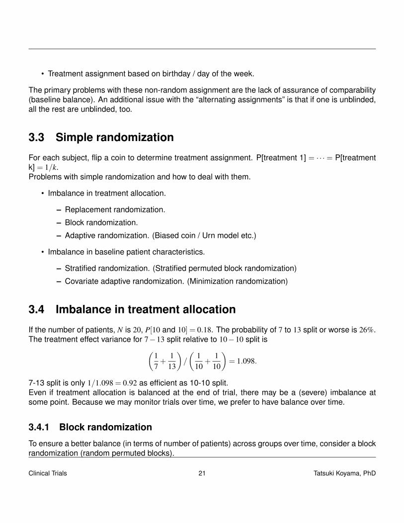
If the number of patients, N is 20, P[10 and 10] = 0.18. The probability of 7 to 13 split or worse is 26%.The treatment effect variance for 7−13 split relative to 10−10 split is(

17+

113

)/

(1

10+

110

)= 1.098.

7-13 split is only 1/1.098 = 0.92 as efficient as 10-10 split.Even if treatment allocation is balanced at the end of trial, there may be a (severe) imbalance atsome point. Because we may monitor trials over time, we prefer to have balance over time.

3.4.1 Block randomization

To ensure a better balance (in terms of number of patients) across groups over time, consider a blockrandomization (random permuted blocks).


Block randomization ensures approximate balance between treatments by forcing balance after asmall number of patients (say 4 or 6). For example, the first 4 patients are allocated to treatment Aor B sequentially based on AABB.There are 6 sequences of A, A, B, B, and let each sequence have 1/6 chance of being selected.

AABB ABAB ABBA BAAB BABA BBAA

for (i in 1:5) {cat(i, sample(rep(LETTERS[1:2], each = 2), 4, replace = FALSE),

"\n")}

1 B A A B2 B B A A3 A A B B4 A B A B5 B A A B

What’s wrong with block size of 2? Block size of 200?Easily applicable to more than 2 groups (A, B, C)

for (i in 1:5) {cat(i, sample(rep(LETTERS[1:3], each = 2), 6, replace = FALSE),

"\n")}

1 C C B B A A2 B C A C A B3 B B A C A C4 A C C B A B5 A C C A B B

Easily applicable to unequal group sizes (Na = 40 and Nb = 20).

for (i in 1:5) {cat(i, sample(rep(LETTERS[1:2], c(4, 2)), 6, replace = FALSE),

"\n")}

1 A B A B A A


2 B A A A B A3 A B A A B A4 B A A A B A5 A B A A A B

Why might we want unequal group sizes?

• We may want to have a better estimate of the effect for the new treatment.

• Treatment costs may be very different.Given the total sample size and the relative cost of treatment 2 to treatment 1, we can find theoptimal allocation ratio to minimize the total cost.

• Variances may be different.Suppose the means, µ1 and µ2, of treatment groups are being compared using

Z =(X1− X2)− (µ1−µ2)√

σ21/n1 +σ2

2/n2

.

For a given N = n1 + n2, the test statistic is maximized when the denominator is minimized.Solving

∂

∂n1

(σ2

1n1

+σ2

2N−n1

)= 0

we get

n1

N=

σ1

σ1 +σ2.

Therefore, the optimal allocation ratio is r = n1/n2 = σ1/σ2.

Analysis should account for the randomization scheme but often does not. Matts and McHugh (1978J Chronic Dis) point out that

• because blocking guarantees balance between groups and increases the power of a study,blocked randomization with the appropriate analysis is more powerful than not blocking at all orblocking and ignoring it in the analysis.

• not accounting for blocking in analysis is conservative.


3.4.2 Biased coin and urn model

These techniques are sometimes classified as “adaptive randomization”.Allocation of i-th patient depends on how many have been randomized to group A (na) and group B(nb).Any given time, the probability of allocation to group A may be

P[A] =nb

na +nb.

Or the rule may be to use P[A] = 2/3 when nb−na > 5, and P[B] = 2/3 when na−nb > 5. Characteristicsof such a randomization scheme are usually studied by simulations.An urn model is one type of biased coin randomization.

• Prepare an urn with one Amber ball and one Blue ball.

• Pick one ball and make the corresponding treatment assignment (A/B).

• Put a ball of the opposite color in the urn.

urn1 <- function(n) {# randomize n patients into A or B. At any time P[A] =# (#B so far + 1) / (#A so far + 1 + #B so far + 1).out <- data.frame(matrix(0, ncol = 4, nrow = n + 1))out[1, 1] <- 1out[1, 2] <- 1for (i in 1:n) {

out[i, 3] <- out[i, 2]/(out[i, 1] + out[i, 2])out[i, 4] <- sample(c("A", "B"), 1, prob = out[i, 2:1])out[i + 1, 1] <- out[i, 1] + (out[i, 4] == "A")out[i + 1, 2] <- out[i, 2] + (out[i, 4] == "B")

}out[, 1] <- out[, 1] - 1out[, 2] <- out[, 2] - 1names(out) <- c("A so far", "B so far", "P[A next]", "Next")out[1:n, ]

}

urn1(n = 10)

A so far B so far P[A next] Next1 0 0 0.500 A


2 1 0 0.333 A3 2 0 0.250 B4 2 1 0.400 B5 2 2 0.500 A6 3 2 0.429 A7 4 2 0.375 B8 4 3 0.444 B9 4 4 0.500 B10 4 5 0.545 A

3.5 Imbalance in baseline patient characteristics

Block randomization and biased coin model ensure that the group sizes are reasonably balanced.In order to facilitate the comparison of treatment effects, balance on important baseline variables issometimes desired.

• Randomization does not guarantee all the measured variables will be balanced. And imbalancedoes not mean randomization did not work.

Senn (1994) It is argued that this practice [testing baseline homogeneity] is philosophically unsound,of no practical value and potentially misleading. Instead it is recommended that prognosticvariables be identified in the trial plan and fitted in an analysis of covariance regardless of theirbaseline distribution (statistical significance).

Piantadosi These methods, while theoretically unnecessary, encourage covariate balance in thetreatment groups, which tends to enhance the credibility of trial results.

An annonymous reviewer Since this is a randomized controlled trial, comparison of baseline char-acteristics (Table 1) is not necessary. The problem with this approach is that when comparingbaseline characteristics we already know that the null hypothesis is true if the randomizationwas done correctly. Thus, we would expect 1 test in 20 to give a ‘significant’ result with p < 0.05by chance alone. The best approach is to specify key prognostic factors to include in multivari-able models irrespective of their significance between treatment groups.

3.5.1 Stratified randomization

Stratified randomization is applied to ensure that the groups are balanced on baseline variables thatare thought to be significant.


• Create strata based on the variables for which balance is sought.e.g., (Male, 65 or younger), (Male, older), (Female, younger), (Female older)

• Randomize to treatments within each stratum. Use block randomization!What’s wrong with

– using simple randomization within a stratum?

– using too many strata?

• Stratification should be accounted for in analysis.

– Pre-randomization stratification and post-randomization stratification (at time of analysis)has no clear winner.

• If trial is large, stratification may not be necessary

• Stratification by center is a good idea from practical viewpoints.

– Allows randomization to be hosted at each site

– Allows sites to be removed and still maintains balance

• Block randomization is a special type of stratified randomization where strata are defined by ....

• If each stratum has a target size, plans need to be in place to close down recruitment based onthe baseline characteristics. e.g., “We do not need any more (Male, older)”.

3.5.2 Adaptive and minimization randomization

Adaptive randomization can be used to reduce baseline imbalance:

• Define an imbalance function based on factors thought to be important

• Then use a rule to define P[treatment A] so that the next assignment is more likely to reduceimbalance.

For example, the factors to balance are sex (male/female) and hypertension (yes/no), and let theimbalance function be

I = 2× (sex imbalance)+3× (hypertension imbalance).

The patients randomized so far are


Sex HypertensionMale Female Yes No

Group 1 10 3 8 5Group 2 8 3 6 5

The next patient is male-non hypertensive. The imbalance will be

I = 2× (11−8)+3× (6−5) = 9 if Group 1,I = 2× (10−9)+3× (6−5) = 5 if Group 2.

Thus let P[Group 2] = 2/3.Minimization randomization uses the same idea but use P[Group 2] = 1, to eliminate randomnesswhen there is some imbalance. Randomize only when to assign the next patient to either group givesthe same value of I.

3.6 Response adaptive randomization

As the name suggests, response adaptive randomization methods use the information about theresponse so far to allocate the next patient.Play the winner: The idea is to allocate more patients in the treatment that seems to be workingbetter. To apply these methods, it is necessary to have a response quickly. Urn model can be usedto make treatment assignment imbalance based on the results (success/failure) of each treatmentso far. (e.g., put one blue ball if the treatment B yields success.)Instead of updating the probabilities of treatment assignment after each patient, we can update themafter a group of patients’ results are available to reduce administrative burden. In a phase II clinicaltrial, play the winner design may be used to reduce the number of treatments in consideration. (e.g.,Only retain the treatment arms that have P[positive response] > 0.4.)

3.6.1 Example: ECMO

Bartlett et al.2 conducted a randomized study of the use of extracorporeal membrane oxygenation(ECMO) to treat newborns with respiratory failure. A play-the-winner design3 was used because

• the outcome is known soon after randomization.

• most ECMO patients were expected to survive and most control patients were expected to die.

– Ethically, the investigators felt obligated not to withhold the lifesaving treatment.

2“Extracorporeal circulation in neonatal respiratory failure: a prospective randomized study”. (1985) Pediatrics3Zelen (1969) JASA; Wei and Durham (1978) JASA


– Scientifically, they felt obligated to perform a randomized study.

The randomization plan:

• The first patient will be randomized to ECMO or the conventional treatment (CT) with equalprobability.

• For each patient who survives on ECMO or dies on CT, one ECMO ball is added to the urn.

• For each patient who survives on CT or dies on ECMO, one CT ball is added to the urn.

• The trial will be terminated when 10 balls of one kind have been added, and that treatment willbe chosen as the winner.

What actually happened:

P(ECMO)=1/2 Patient 1 was randomized to ECMO and survived.

P(ECMO)=2/3 Patient 2 was randomized to CT and died.

P(ECMO)=3/4 Patient 3 was randomized to ECMO and survived








Randomization was stopped when there were 11 ECMO patients who survived and 1 CT patient whodied.Controversies followed because ...

fisher.test(cbind(c(11, 0), c(0, 1)))


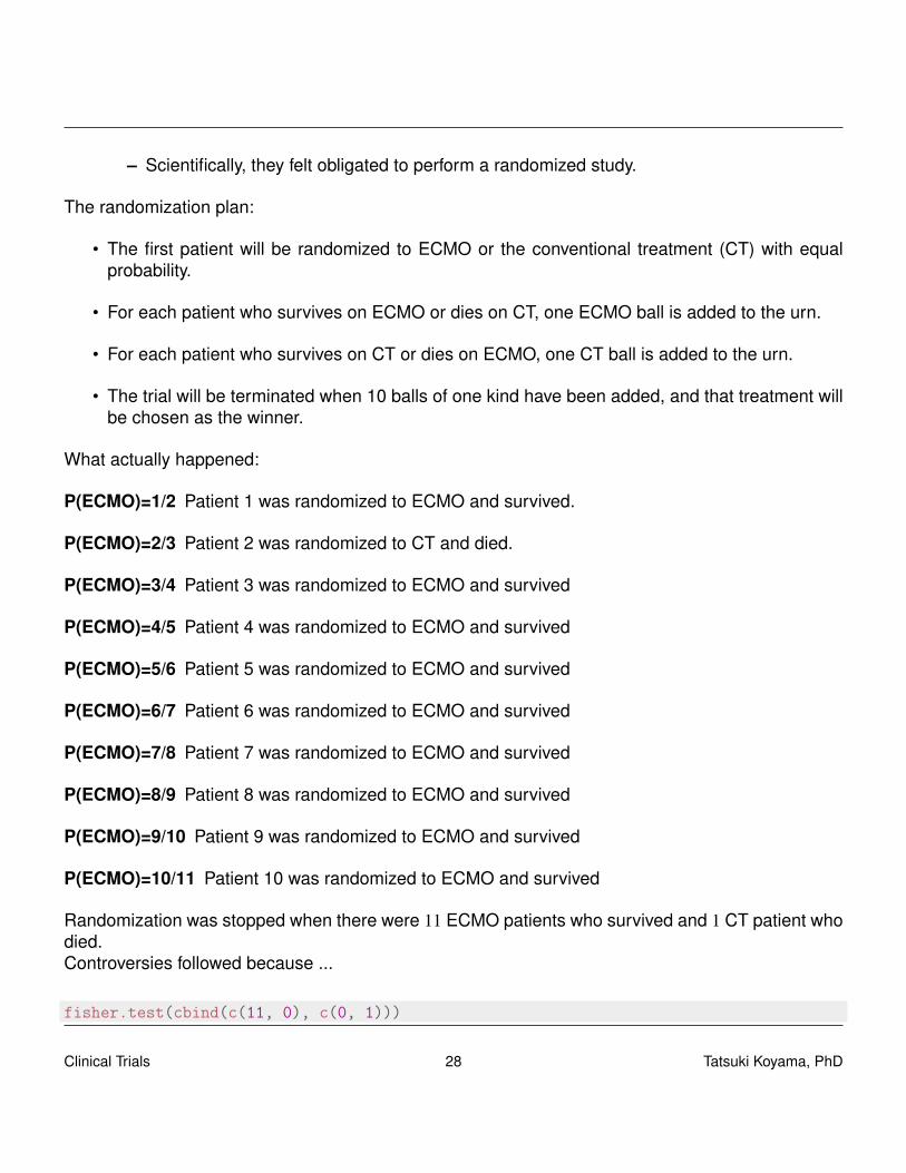
Fisher's Exact Test for Count Data

data: cbind(c(11, 0), c(0, 1))p-value = 0.08alternative hypothesis: true odds ratio is not equal to 195 percent confidence interval:0.282 Inf

sample estimates:odds ratio

Inf

“In retrospect it would have been better to begin with two or three pairs of balls, which probably wouldhave resulted in more than one control patient.”

3.7 Nonbipartite matching in clinical trials

• Reference: Lu B, Greevy R, Xu X, Beck C. “Optimal nonbipartite matching and its statisticalapplications”. 2011. 65(1):21-30.

• R package “nbpMatching”http://biostat.mc.vanderbilt.edu/wiki/Main/MatchedRandomization

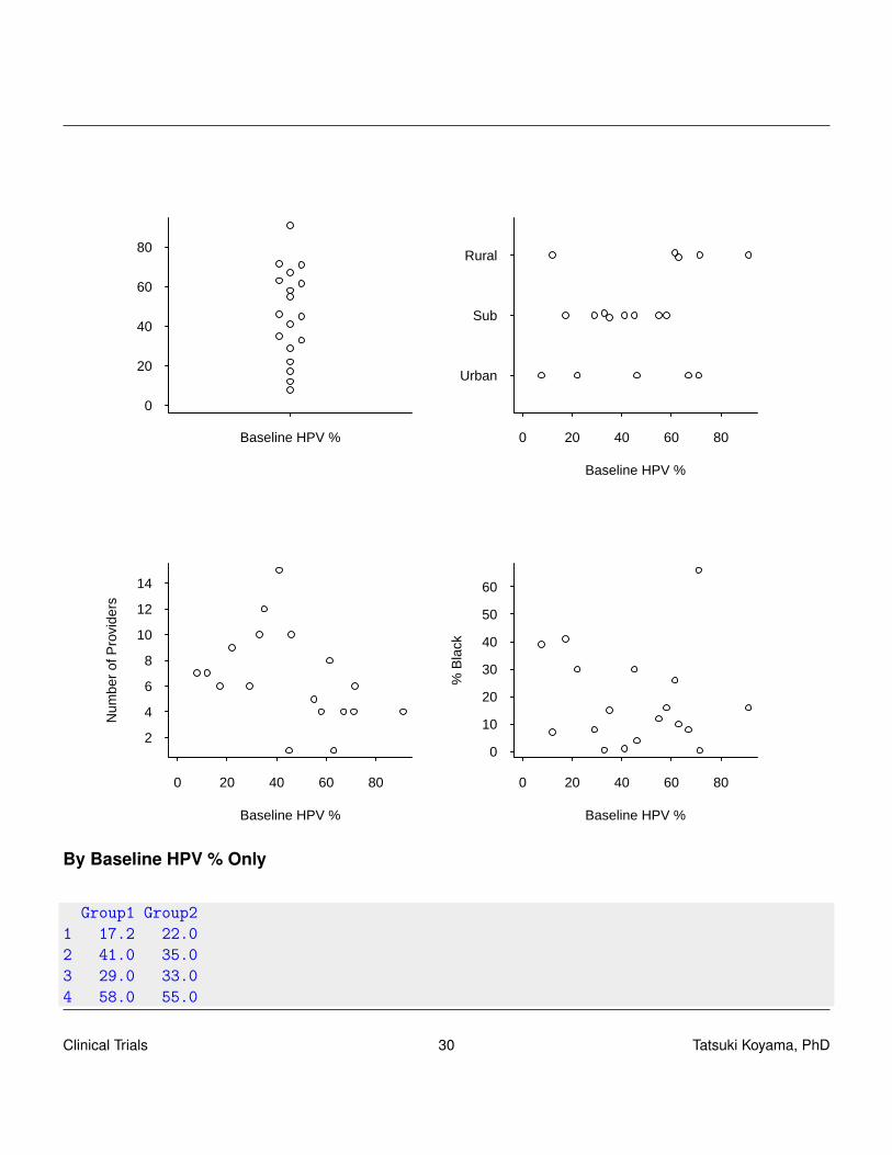
When baseline data on all the subjects are available, the subjects can be matched, and treatmentsare randomly assigned within each pair. Matching is done to minimize some form of multidimensional(multivariate) distance, e.g., Mahalanobis distance.

3.7.1 Example

The human papillomavirus (HPV) vaccine will prevent a high proportion of vaginal, oropharyngeal,vulvar, and penile cancers. Yet the proportion of 11- and 12-year old girls who receive this vaccine isnot very high. The investigators would like to test effectiveness of the tailored coaching interventionto educate the health-care providers. For this study, 18 community-based, private pediatric practiceshave been recruited.


Baseline HPV %

0

20

40

60

80

Urban

Sub

Rural

0 20 40 60 80

Baseline HPV %

0 20 40 60 80

2

4

6

8

10

12

14

Baseline HPV %

Num

ber

of P

rovi

ders

0 20 40 60 80

0

10

20

30

40

50

60

Baseline HPV %

% B

lack

By Baseline HPV % Only

Group1 Group21 17.2 22.02 41.0 35.03 29.0 33.04 58.0 55.0


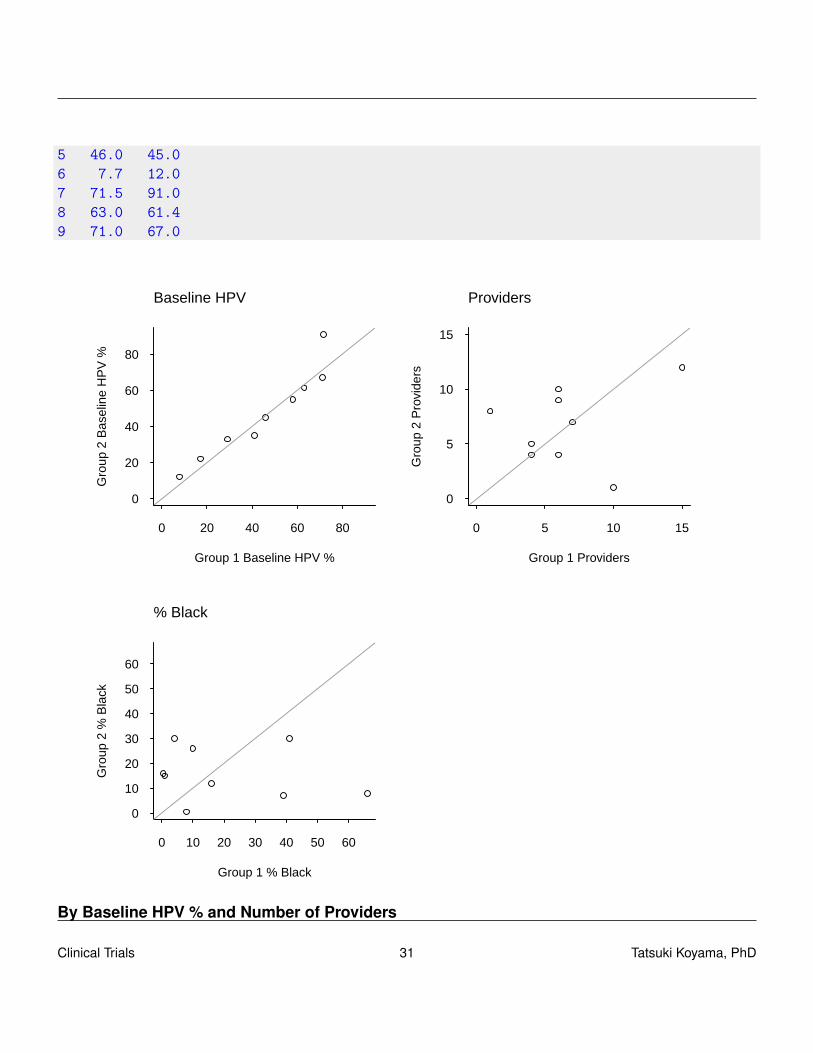
5 46.0 45.06 7.7 12.07 71.5 91.08 63.0 61.49 71.0 67.0

0 20 40 60 80

0

20

40

60

80

Group 1 Baseline HPV %

Gro

up 2

Bas

elin

e H

PV

%

Baseline HPV

0 5 10 15

0

5

10

15

Group 1 Providers

Gro

up 2

Pro

vide

rs

Providers

0 10 20 30 40 50 60

0

10

20

30

40

50

60

Group 1 % Black

Gro

up 2

% B

lack

% Black

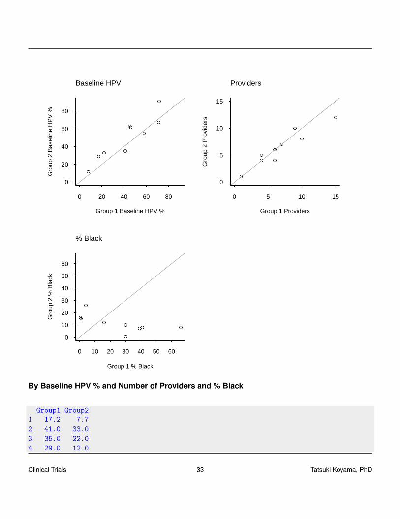
By Baseline HPV % and Number of Providers


Group1 Group21 17.2 29.02 41.0 35.03 22.0 33.04 58.0 55.05 46.0 61.46 7.7 12.07 45.0 63.08 71.5 91.09 71.0 67.0


0 20 40 60 80

0

20

40

60

80


Gro

up 2

Bas

elin

e H

PV

%

Baseline HPV

0 5 10 15

0

5

10

15

Group 1 ProvidersG

roup

2 P

rovi

ders

Providers

0 10 20 30 40 50 60

0

10

20

30

40

50

60

Group 1 % Black

Gro

up 2

% B

lack

% Black

By Baseline HPV % and Number of Providers and % Black

Group1 Group21 17.2 7.72 41.0 33.03 35.0 22.04 29.0 12.0


5 58.0 55.06 46.0 61.47 45.0 63.08 71.5 67.09 71.0 91.0

0 20 40 60 80

0

20

40

60

80


Gro

up 2

Bas

elin

e H

PV

%

Baseline HPV

0 5 10 15

0

5

10

15

Group 1 Providers

Gro

up 2

Pro

vide

rs

Providers

0 10 20 30 40 50 60

0

10

20

30

40

50

60

Group 1 % Black

Gro

up 2

% B

lack

% Black


Chapter 4

Superiority, Non-inferiority, and equivalence

4.1 Superiority and non-inferiority

In a phase 3 clinical trial, the objective is often to show the new treatment is better than the con-ventional treatment. This is called a superiority clinical trial, in which the following hypotheses aretested:

HS0 : δ = 0HS1 : δ > 0

where δ is the difference of the treatment effects. Here we assume larger values of δ indicate afavorable result. We generally do not conduct a two-sided hypothesis test in a clinical trial. Type Ierror rate is usually set at 2.5%, and power is usually set at 80% or 90% at some clinically meaningfulvalue, δS.When there is a conventional treatment that is known to be effective, it may be of interest to shownon-inferiority of the new treatment to the control.

HN0 : δ =−δI

HN1 : δ >−δI

Here, δI is a pre-specified positive number, which is referred to as the non-inferiority margin. It iscustomary to set the power of non-inferiority test at 0. Mathematically, superiority testing and non-inferiority testing are very similar; one is a location shift of the other.After observing the data, δ , it is always possible to compute δI such that H0 for the non-inferiority testis rejected. Therefore, it is necessary to define the non-inferiority margin a priori.A non-inferiority trial usually requires a bigger sample size than a superiority trial does. That is,δI < δS. δI needs to be small enough to be clinically indifferent, and δS needs to be large enough tobe clinically meaningful.


Because when the data from the control and treatment groups are similar, it biases towards nodifference, the intention-to-treat analysis biases towards positive results in a non-inferiority trial. Thiscan be seen in the following small simulation study.

sig <- 4del <- 1alp <- 0.025bet <- 0.1

(n <- ceiling(2 * (qnorm(alp) + qnorm(bet))^2 * sig^2/del^2))

[1] 337

supSim <- function(B, n, mu0, mu1, sig, pSwitch = 0) {# pSwitch is the proportion of patients switching the# group (T -> C and C -> T are the same.)nSwitch <- ceiling(n * pSwitch)toSwitch <- sample(1:n, nSwitch)X0 <- Y0 <- matrix(rnorm(B * n, mu0, sig), ncol = B)X1 <- Y1 <- matrix(rnorm(B * n, mu1, sig), ncol = B)

for (i in toSwitch) {X0[i, ] <- Y1[i, ]X1[i, ] <- Y0[i, ]

}XBar0 <- apply(X0, 2, mean)XBar1 <- apply(X1, 2, mean)

zVal <- sqrt(n) * (XBar1 - XBar0)/(sqrt(2) * sig)pVal <- 1 - pnorm(zVal)table(pVal < 0.025)

}(supSim0.0 <- supSim(B = 10000, n = n, mu0 = 0, mu1 = 0, sig = 4))

FALSE TRUE9786 214

(supSim1.0 <- supSim(B = 10000, n = n, mu0 = 0, mu1 = 1, sig = 4))

FALSE TRUE1077 8923


(supSim0.1 <- supSim(B = 10000, n = n, mu0 = 0, mu1 = 0, sig = 4,pSwitch = 0.2))

FALSE TRUE9743 257

(supSim1.1 <- supSim(B = 10000, n = n, mu0 = 0, mu1 = 1, sig = 4,pSwitch = 0.2))

FALSE TRUE5163 4837

niSim <- function(B, n, del, niMargin = 1, sig, pSwitch = 0) {# del is the true difference (>0). Under null,# del=-niMargin; under alternative, del=0. pSwitch is# the proportion of patients switching the group (T -># C and C -> T are the same.)nSwitch <- ceiling(n * pSwitch)toSwitch <- sample(1:n, nSwitch)X0 <- Y0 <- matrix(rnorm(B * n, 0, sig), ncol = B) # controlX1 <- Y1 <- matrix(rnorm(B * n, -del, sig), ncol = B) # new treatment

for (i in toSwitch) {X0[i, ] <- Y1[i, ]X1[i, ] <- Y0[i, ]

}XBar0 <- apply(X0, 2, mean)XBar1 <- apply(X1, 2, mean)

zVal <- sqrt(n) * (XBar1 - XBar0 + niMargin)/(sqrt(2) * sig)pVal <- 1 - pnorm(zVal)table(pVal < 0.025)

}(niSim0.0 <- niSim(B = 10000, n = n, del = 1, niMargin = 1, sig = 4))

FALSE TRUE9764 236


(niSim1.0 <- niSim(B = 10000, n = n, del = 0, niMargin = 1, sig = 4))

FALSE TRUE984 9016

(niSim0.1 <- niSim(B = 10000, n = n, del = 1, niMargin = 1, sig = 4,pSwitch = 0.2))

FALSE TRUE7397 2603

(niSim1.1 <- niSim(B = 10000, n = n, del = 0, niMargin = 1, sig = 4,pSwitch = 0.2))

FALSE TRUE1021 8979

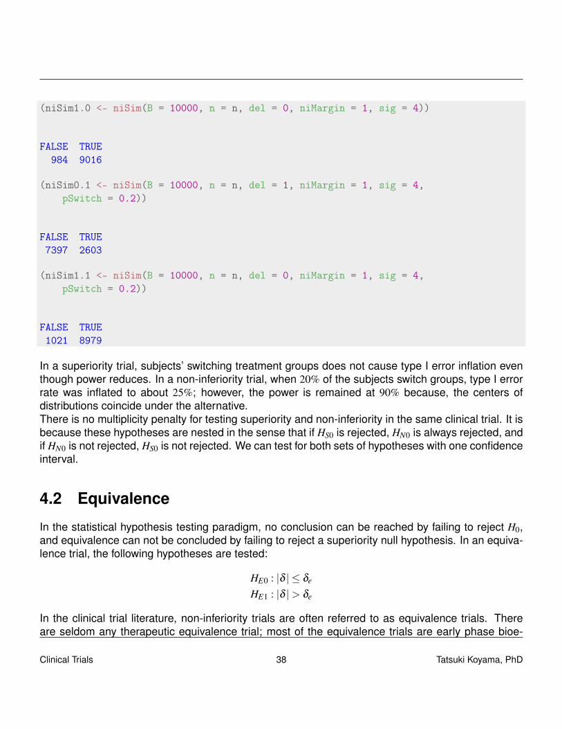
In a superiority trial, subjects’ switching treatment groups does not cause type I error inflation eventhough power reduces. In a non-inferiority trial, when 20% of the subjects switch groups, type I errorrate was inflated to about 25%; however, the power is remained at 90% because, the centers ofdistributions coincide under the alternative.There is no multiplicity penalty for testing superiority and non-inferiority in the same clinical trial. It isbecause these hypotheses are nested in the sense that if HS0 is rejected, HN0 is always rejected, andif HN0 is not rejected, HS0 is not rejected. We can test for both sets of hypotheses with one confidenceinterval.

4.2 Equivalence

In the statistical hypothesis testing paradigm, no conclusion can be reached by failing to reject H0,and equivalence can not be concluded by failing to reject a superiority null hypothesis. In an equiva-lence trial, the following hypotheses are tested:

HE0 : |δ | ≤ δe

HE1 : |δ |> δe

In the clinical trial literature, non-inferiority trials are often referred to as equivalence trials. Thereare seldom any therapeutic equivalence trial; most of the equivalence trials are early phase bioe-


quivalence trials in the pharmacokinetics/pharmacodinamics arena. In bioequivalence trials, severalpharmacokinetic (PK) parameters, such as, Cmax, Cmin, and AUC for a generic drug are compared tothose for the marketed drug.

An example of clinical equivalence trialPri et. al “Leukotriene antagonists as first-line or add-on asthma-controller therapy”. New Eng-land Journal of Medicine (2011). In this pragmatic clinical trial, the investigators aimed to showleukotrine-receptor antagonist (LTRA) is equivalent to either an inhaled glucocorticoid for first-lineasthma-controller therapy or a long-acting beta agonist (LABA) as add-on therapy in patients alreadyreceiving inhaled glucocorticoid therapy. This is a pragmatic trial, as well. As with non-inferioritytrials, the intention-to-treat analysis biases towards equivalence, making it challenging to handledropouts and non-compliances (switching treatment arms).


Chapter 5

Phase II Oncology Clinical Trials

5.1 Introduction

Phase II clinical trial A clinical trial designed to test the feasibility of, and level of activity of, a newagent or procedure. (safety and activity)

Some typical characteristics of a typical phase II clinical trial include:

• It includes a placebo and two to four doses of the test drug.

• When the response is observed quickly, adaptive designs may be beneficial and used becausethey may

– improve quality of estimation of the MED (minimum effective dose (lowest dose of a drugthat produces the desired clinical effect).

– increase number of patients allocated to MED.

– allow for early stopping for futility.

The primary objectives of phase II trials are:

• To determine whether the drug is worthy of further study in phase III trial. Significant treatmenteffect? / dose-response relationship?

• To gather information to help design phase III trial.

– Determine dose(s) to carry forward

– Determine the primary and secondary endpoints

– Estimate treatment effects for power/sample size analysis

– Estimate recruitment rate


– Examine feasibility of treatment (logistics of administration and cost)– Learn about side effects and toxicity

In phase II clinical trials, parallel group designs, crossover designs, and factorial designs are oftenused.

5.2 Phase II trials in oncology

A phase II clinical trial in oncology generally uses a fixed dose chosen in a phase I trial. The primaryobjective is to assess therapeutic response to treatment. In the simplest case, a single treatmentarm is compared to a historical control. In other cases, a control group and/or multiple doses areincluded.The treatment efficacy is often evaluated on surrogate markers for a timely (quick) evaluation ofefficacy.

Surrogate outcome An outcome measurement in a clinical trial that substitutes for a definitive clin-ical outcome or disease status.

• CD4 counts in AIDS study.• PSA (prostatic specific antigen) in prostate cancer study.• Blood pressure in cardiovascular disease.• 3 months survival (binary) for survival.• Tumor shrinkage for survival.

Tumor response to treatment is evaluated according to Response Evaluation Criteria in Solid Tumors(RECIST)

Complete response (CR) Disappearance of all target lesions.

Partial response (PR) At least a 30% decrease in the sum of the longest diameter (LD) of targetlesions, taking as reference the baseline sum LD.

Stable disease (SD) Neither sufficient shrinkage to qualify for PR nor sufficient increase to qualifyfor PD, taking as reference the smallest sum LD since the treatment started.

Progressive disease (PD) At least a 20% increase in the sum of the LD of target lesions, taking asreference the smallest sum LD recorded since the treatment started or the appearance of oneor more new lesions.

Generally, objective tumor response is defined as CR or PR in RECIST so that the response variablehas a binary endpoint. In the rest of chapter, we will consider a single arm trial with a binary response.The hypothesis of interest is one-sided H1 : p > p0, and the type I error rate is usually 5 to 10%. Thepower is usually 80 to 90%.


5.3 Classical (old) two-stage designs

It is crucial that these phase II studies have an opportunity to stop early for toxicity, and that is ac-complished by Data Monitoring Committee (DMC), aka, Data and Safety Monitoring Board (DSMB).It is also desired to discard ineffective treatment early, and two-stage designs with a futility stop hasbeen popular.We will discuss the designs proposed by Gehan (1961), Fleming (1982), and Simon (1989), usingthe following unified notation:

• stage I sample size · · ·n1.

• stage I data · · ·X1 ∼ Binomial(n1, p).

• stage I critical value · · ·r1 so that if X1 ≤ r1 then terminate the study for futility.

• stage II sample size · · ·n2.

• stage II data · · ·X2 ∼ Binomial(n2, p).

• total sample size · · ·nt = n1 +n2.

• total data · · ·Xt ≡ X1 +X2.

• stage II critical value · · ·rt so that if Xt ≤ rt then terminate the study for futility, otherwise concludeefficacy.

5.3.1 Gehan’s design

It is old (1961) and outdated but may be ok to use in limited situations. The design calls for the firststage with n1 = 14 and r1 = 0, i.e., if no positive response is observed in 14, then stop for futility. Therational is that if true response rate is at least 20%, then X1 = 0 is unlikely. In fact, it is 0.044. Thesecond stage sample size depends on the desired precision for estimating p, and it ranges between1 and 86. A typical n2 is 14 so that nt = 28.

5.3.2 Fleming’s design

Fleming (1982) proposed a multistage design for phase II clinical trials. One of its key characteristicsis stopping early for efficacy.ExampleH0 : p = 0.15, H1 : p = 0.30. (powered at 0.30)α = .05, β = .2(Reject H0 in stage 1 if X1 ≥ s1.


n1 r1 s1 nt rt α 1−β E0[N] E1[N]29 4 9 47 10 0.0490 0.8013 36.6 36.9

5.4 Simon’s design

In his 1989 paper, Simon introduced two criteria to choose a 2 stage design for single arm and onesided test. The optimal design has the smallest expected sample size under H0 (n1 +Ep0[n2]), andthe minimax design has the smallest total sample size (n1 +n2). For p0 = 0.15 and p1 = 0.30,

n1 r1 nt rt α 1−β E0[N] pet0 E1[N] pet1optimal 19 3 55 12 0.048 0.801 30.4 0.68 50.2 0.13

minimax 23 3 48 11 0.046 0.804 34.5 0.54 46.7 0.05single stage −− −− 48 11 0.048 0.819 48.0 0.00 48.0 0.00

5.4.1 Conditional power

To find a good design (sample sizes and critical values), we need to understand the conditionalpower of a design. The conditional power is the probability of rejecting H0 (in stage 2) given thestage 1 result, i.e., conditioned on X1 = x1. Clearly, when X1 > rt , conditional power is 1, and whenX1 ≤ r1 (futility stop), conditional power is 0.

CP(x1) = P[Reject in stage 2|x1] = P[x1 +X2 > rt |x1]

= P[X2 > rt− x1|x1]

=n2

∑x2=rt−x1+1

(n2

x2

)px2(1− p)n2−x2

Conditional power is a function of p, x1 and n2 as well as rtTo obtain the unconditional power, we need to integrate (sum) the conditional power over all possiblex1 values.

ρ(p) =n1

∑x1=0

CP(x1)Pp[X1 = x1]

ρ(p) =n1

∑x1=r1+1

CP(x1)

(n1

x1

)px1(1− p)n1−x1.

Given α and β a design is chosen so that ρ(p0)≤ α and ρ(p1)≥ 1−β .


Unlike in a single-stage situation, there may be more than one good design. Simon used the optimaland minimax to choose two reasonable designs among many satisfying the type I error rate andpower constraints.Expected sample size under the null can be written as

Ep0[nt ] = n1 +n2P[continue to stage 2|p0]

= n1 +n2×P[X1 > r1|p0]

= n1 +n2×n1

∑x1=r1+1

(n1

x1

)px1

0 (1− p0)n1−x1.

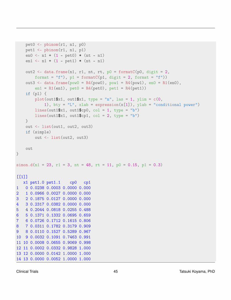
5.4.2 Computing design characteristics

simon.d <- function(n1, r1, nt, rt, p0, p1, pl = TRUE, simple = FALSE) {# x1 <= r1 stop for futility xt <= rt conclude futilityR4 <- function(x) {

round(x, 4)}R1 <- function(x) {

round(x, 1)}

x1 <- 0:n1pst1.0 <- dbinom(x1, n1, p0)pst1.1 <- dbinom(x1, n1, p1)

cp0 <- 1 - pbinom(rt - x1, nt - n1, p0)cp1 <- 1 - pbinom(rt - x1, nt - n1, p1)cp0[x1 <= r1] <- 0cp1[x1 <= r1] <- 0cp0[x1 > rt] <- 1cp1[x1 > rt] <- 1

pow0 <- sum(pst1.0 * cp0)pow1 <- sum(pst1.1 * cp1)

keep <- pmax(pst1.0, pst1.1) > 0.00009out1 <- data.frame(x1 = R4(x1), pst1.0 = R4(pst1.0), pst1.1 = R4(pst1.1),

cp0 = R4(cp0), cp1 = R4(cp1))[keep, ]


pet0 <- pbinom(r1, n1, p0)pet1 <- pbinom(r1, n1, p1)en0 <- n1 + (1 - pet0) * (nt - n1)en1 <- n1 + (1 - pet1) * (nt - n1)

out2 <- data.frame(n1, r1, nt, rt, p0 = formatC(p0, digit = 2,format = "f"), p1 = formatC(p1, digit = 2, format = "f"))

out3 <- data.frame(pow0 = R4(pow0), pow1 = R4(pow1), en0 = R1(en0),en1 = R1(en1), pet0 = R4(pet0), pet1 = R4(pet1))

if (pl) {plot(out1$x1, out1$x1, type = "n", las = 1, ylim = c(0,

1), bty = "L", xlab = expression(x[1]), ylab = "conditional power")lines(out1$x1, out1$cp0, col = 1, type = "b")lines(out1$x1, out1$cp1, col = 2, type = "b")

}out <- list(out1, out2, out3)if (simple)

out <- list(out2, out3)

out}

simon.d(n1 = 23, r1 = 3, nt = 48, rt = 11, p0 = 0.15, p1 = 0.3)

[[1]]x1 pst1.0 pst1.1 cp0 cp1

1 0 0.0238 0.0003 0.0000 0.0002 1 0.0966 0.0027 0.0000 0.0003 2 0.1875 0.0127 0.0000 0.0004 3 0.2317 0.0382 0.0000 0.0005 4 0.2044 0.0818 0.0255 0.4886 5 0.1371 0.1332 0.0695 0.6597 6 0.0726 0.1712 0.1615 0.8068 7 0.0311 0.1782 0.3179 0.9099 8 0.0110 0.1527 0.5289 0.96710 9 0.0032 0.1091 0.7463 0.99111 10 0.0008 0.0655 0.9069 0.99812 11 0.0002 0.0332 0.9828 1.00013 12 0.0000 0.0142 1.0000 1.00014 13 0.0000 0.0052 1.0000 1.000


15 14 0.0000 0.0016 1.0000 1.00016 15 0.0000 0.0004 1.0000 1.000

[[2]]n1 r1 nt rt p0 p1

1 23 3 48 11 0.15 0.30

[[3]]pow0 pow1 en0 en1 pet0 pet1

1 0.0455 0.803 34.5 46.7 0.54 0.0538


0 5 10 15

0.0

0.2

0.4

0.6

0.8

1.0

x1

cond

ition

al p

ower

Given a design, computing operational characteristics such as type I error rate, power, expectedsample size is not difficult; however, solving for the optimal, minimax, and other preferable designsis not trivial. Simon’s original papers show how to do this.

A very good webpage by Anastasia Ivanova at UNC is at http://cancer.unc.edu/biostatistics/program/ivanova/SimonsTwoStageDesign.aspx.


5.4.3 Something in between

The two criteria, optimal and minimax, give two designs that are extreme, and neither may fit theinvestigators’ needs. For example, for testing H0 : p = 0.3 with α = 0.05 and β = 0.10 at p1 = 0.45, theoptimal design and minimax designs are:

n1 r1 nt rt α 1−β E0[N] pet0optimal 40 13 110 40 0.048 0.901 60.8 0.70

balanced 53 18 106 39 0.043 0.903 64.4 0.78minimax 77 27 88 33 0.050 0.901 78.5 0.86

The optimal design tends to have a small n1 and the minimax design tends to have a large n1.Therefore, a simple approach to find a good alternative design is to force n1 = n2. (balanced designof Ye and Shyr, 2007)

simon.d(n1 = 40, r1 = 13, nt = 110, rt = 40, p0 = 0.3, p1 = 0.45,pl = FALSE, simple = TRUE)

[[1]]n1 r1 nt rt p0 p1

1 40 13 110 40 0.30 0.45


1 0.0482 0.901 60.8 105 0.703 0.0751


[[1]]n1 r1 nt rt p0 p1

1 53 18 106 39 0.30 0.45


1 0.0431 0.903 64.4 102 0.784 0.0687

A more systematic approach is to express the criteria for optimization as

q(w) = w× (nt)+(1−w)×E0[N],

where 0 ≤ w ≤ 1. q(0) and q(1) correspond to the optimal and minimax designs, respectively. Com-putation shows that the minimax design is the best design with respect to q(w) for w ∈ (0.827,1]. In


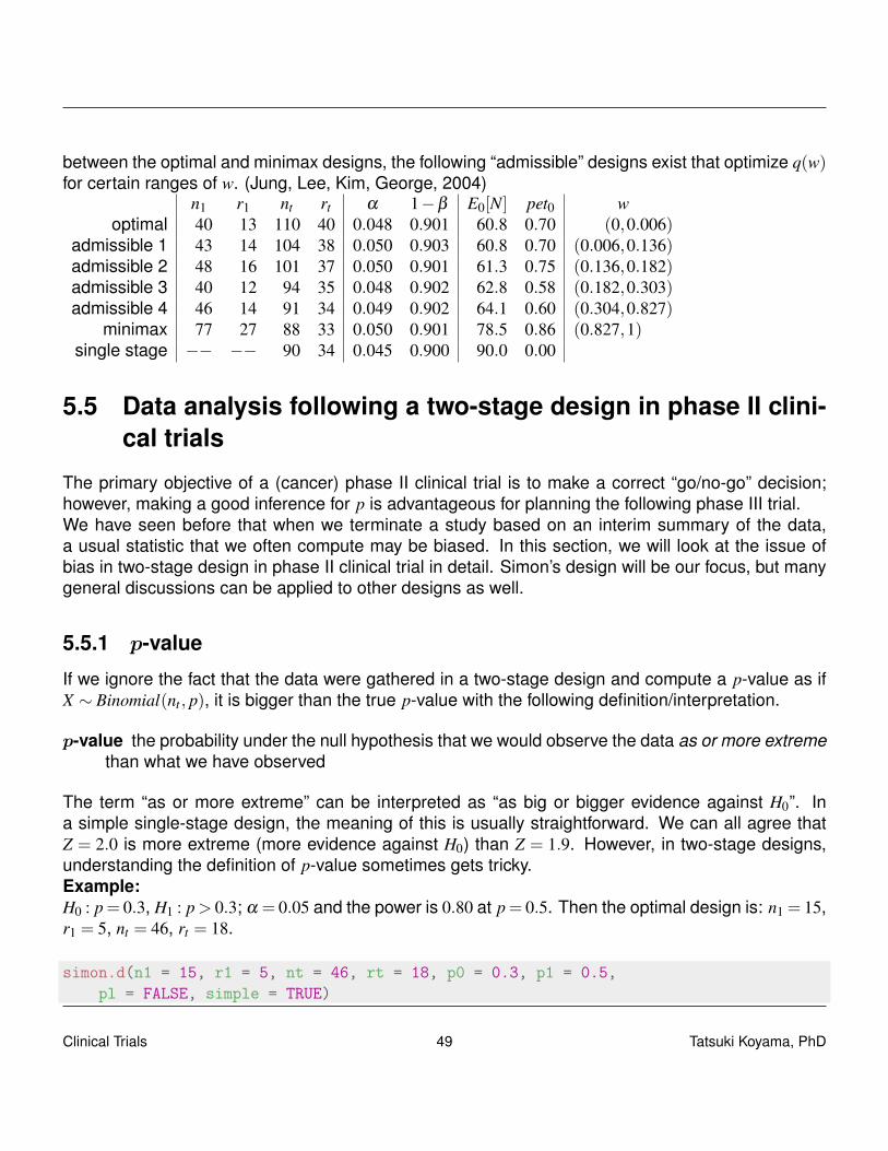
between the optimal and minimax designs, the following “admissible” designs exist that optimize q(w)for certain ranges of w. (Jung, Lee, Kim, George, 2004)

n1 r1 nt rt α 1−β E0[N] pet0 woptimal 40 13 110 40 0.048 0.901 60.8 0.70 (0,0.006)

admissible 1 43 14 104 38 0.050 0.903 60.8 0.70 (0.006,0.136)admissible 2 48 16 101 37 0.050 0.901 61.3 0.75 (0.136,0.182)admissible 3 40 12 94 35 0.048 0.902 62.8 0.58 (0.182,0.303)admissible 4 46 14 91 34 0.049 0.902 64.1 0.60 (0.304,0.827)

minimax 77 27 88 33 0.050 0.901 78.5 0.86 (0.827,1)single stage −− −− 90 34 0.045 0.900 90.0 0.00

5.5 Data analysis following a two-stage design in phase II clini-cal trials

The primary objective of a (cancer) phase II clinical trial is to make a correct “go/no-go” decision;however, making a good inference for p is advantageous for planning the following phase III trial.We have seen before that when we terminate a study based on an interim summary of the data,a usual statistic that we often compute may be biased. In this section, we will look at the issue ofbias in two-stage design in phase II clinical trial in detail. Simon’s design will be our focus, but manygeneral discussions can be applied to other designs as well.

5.5.1 p-value

If we ignore the fact that the data were gathered in a two-stage design and compute a p-value as ifX ∼ Binomial(nt , p), it is bigger than the true p-value with the following definition/interpretation.

p-value the probability under the null hypothesis that we would observe the data as or more extremethan what we have observed

The term “as or more extreme” can be interpreted as “as big or bigger evidence against H0”. Ina simple single-stage design, the meaning of this is usually straightforward. We can all agree thatZ = 2.0 is more extreme (more evidence against H0) than Z = 1.9. However, in two-stage designs,understanding the definition of p-value sometimes gets tricky.Example:H0 : p= 0.3, H1 : p> 0.3; α = 0.05 and the power is 0.80 at p= 0.5. Then the optimal design is: n1 = 15,r1 = 5, nt = 46, rt = 18.



[[1]]n1 r1 nt rt p0 p1

1 15 5 46 18 0.30 0.50


1 0.0499 0.803 23.6 41.3 0.722 0.151

Now suppose we observe X1 = 7 in stage 1 so that we move on to the second stage. And in stage 2,we observe additional 12 positive responses in n2 = 31 patients (19 in 46 total) so that H0 is rejectedbecause Xt = 19 > rt .If we compute a p-value without taking into account the study design, we might use X ∼Binomial(46,0.3)and compute

pc = P0[X ≥ 19] =46

∑i=19

(46i

)0.3i(1−0.3)46−i

where pc is a conventional p-value. H0 is rejected but this p-value is greater than α as shown below:

1 - pbinom(18, 46, 0.3)

[1] 0.0681

To see this inconsistency clearly, we will rewrite above as

pc = P0[X ≥ 19]

=15

∑x1=0

P0[X2 ≥ 19− x1|X1 = x1]P0[X1 = x1].

From this expression we see that in computing pc, we include sample paths that can not be realizedwith this Simon’s design, namely, X1 = 0, X2 ≥ 19; X1 = 1, X2 ≥ 18; · · · ; X2 = 5, X2 ≥ 14. A properp-value that takes into account the actual sampling scheme used may be

pp =15

∑x1=6

P0[X2 ≥ 19− x1|X1 = x1]P0[X1 = x1].


In general, for Simon-like two-stage designs, p-value should be calculated

pp =n1

∑x1=r1+1

P0[X2 ≥ xt− x1|X1 = x1]P0[X1 = x1],

if x1 > r1 (i.e., if there is a second stage).The following simple R script computes this p-value:

pp <- function(n1, r1, nt, rt, x1, xt, p0) {x1v <- (r1 + 1):n1p.val <- sum((1 - pbinom(xt - x1v - 1, (nt - n1), p0)) *

dbinom(x1v, n1, p0))pc <- 1 - pbinom(xt - 1, nt, p0)if (x1 <= r1) {

p.val <- pc <- 1 - pbinom(x1 - 1, n1, p0)}c(p.val = p.val, pc = pc)

}

pp(n1 = 15, r1 = 5, nt = 46, rt = 18, x1 = 7, xt = 19, p0 = 0.3)

p.val pc0.0499 0.0681

When x1 ≤ r1 so that the trial is terminated in stage 1, we can define

pp = P0[X1 ≥ x1].

Thus we think that “moving on to the second stage” has more evidence against H0 than “terminatingin the first stage for futility”, which makes sense.The proper p-value (pp) has the following characteristics:

• It is always smaller than or equal to pc.

• It is consistent with the hypothesis testing, i.e., pp ≤ α if and only if H0 is rejected.

• If Xt = rt +1, then pp is equal to the level of the test (so-called the actual type I error rate).

• It does not distinguish different sample paths that lead to the same Xt . That is, evidence againstH0 is identical if xt is the same regardless of x1.For example, X1 = 8, X2 = 12 and X1 = 10, X2 = 10 yield the same p-values.


When does this (pp) break down?It breaks down when we allow n2 to be different for various values of X1. In some modifications ofSimon’s design (e.g., Banerjee A, Tsiatis AA. Stat Med 2006), the stage 2 sample size varies withx1. Then, pp can not be computed because we cannot order the sample paths simply based on Xt .A bigger concern is that this pp cannot be used when n2 is changed from that planned. An evenbigger concern is if the actual n2 is different from that planned, how can we re-compute the criticalvalue, rt , to control type I error rate? The answer is not simple!

5.5.2 Point estimate

Because the results from a phase II clinical trial are often used in planning a phase III clinical trial, agood estimate of p is often of interest.

MLE

In a single stage design, the MLE of p is p = x/n. For a Simon’s design, we can write the likelihood,letting Yi denote the individual datum from a Bernoulli(p) population, as follows:

L(p|Y ) =

{Π

n1i=1 pyi(1− p)1−yi if ∑

n1i yi ≤ r1

Πnti=1 pyi(1− p)1−yi if ∑

n1i y1 > r1

l(p|X) =

{x1log(p)+(n1− x1)log(1− p) if x1 ≤ r1

xt log(p)+(nt− xt)log(1− p) if x1 > r1

Therefore, the MLE for π is

p(x) =

{x1/n1 if x1 ≤ r1

xt/nt if x1 > r1

We have seen before that this p(x) has a downward bias, i.e., Ep[p(x)] ≤ p. A simple explanation isthat when p is small at the end of stage 1, we tend to terminate the study, and this downward biastends to remain; however when p is large at the end of stage 1, more data are gathered and theupward bias of stage 1 tends to be corrected.Example: p0 = 0.3, p1 = 0.5, α = 0.05, β = 0.2. Then the minimax design is (n1 = 19, r1 = 6, nt = 39,rt = 16). Further suppose X1 = 8 and X2 = 12 so that Xt = 20.

p =2039

= 0.513.


Whitehead

We can write the bias of the MLE estimator as:

B(p) = Ep[p(x)]− p.

So a good estimator would be

p = p−B(p).

However, B(p) is unknown, so we need to estimate it. Let’s use the current estimate of p in B(p).That is

pw = p−B(pw).

This is Whitehead’s estimator (1986 Biometrika). We can write

pw = p−Epw [p(x)]+ pw,

which leads to

Epw [p(x)] = p.

To find pw, we need to numerically solve for pw that satisfies

Epw [p(x)] =r1

∑x1=0

x1

n1P[X1 = x1|p = pw]+

n1

∑x1=r1+1

n2

∑x2=0

x1 + x2

ntP[X1 = x1|p = pw]P[X2 = x2|p = pw]

= p

In the current example, pw = 0.520.

Koyama

We can write the bias of the MLE estimator as:

B(p) = Ep[p(x)]− p.

So a good estimator would be

p = p−B(p).


However, B(p) is unknown, so let’s use B(p), that is

pk = p−B(p).

This is simpler and more straightforward than Whitehead’s estimator. We can write

pk = p−Ep[p(x)]+ p= 2p−E p[p(x)].

Solving for pk is considerably easier. First compute

Ep[p(x)] =r1

∑x1=0

x1

n1P[X1 = x1|p = p]+

n1

∑x1=r1+1

n2

∑x2=0

x1 + x2

ntP[X1 = x1|p = p]P[X2 = x2|p = p],

then subtract it from 2 p. In the current example, pk = 0.521.

Unbiased estimator

For a general multistage design with early stopping for futility and efficacy, Jung and Kim (2004 StatMed) found the unbiased estimator of p. They showed that the pair (M,S), where M is the numberof stage (when terminated) and S the number of successes, is complete and sufficient for p. Andclearly x1/n1 is unbiased for p, the uniformly minimum variance unbiased estimator (UMVUE) is foundthrough Rao-Blackwell theorem.

The expression for pub is complex, but for Simon’s two-stage design (two-stage with only futility stop),it can be written as

pub =∑

n1∧xtx1=(r1+1)∨(xt−n2)

(n1−1x1−1

)( n2xt−x1

)∑

n1∧xtx1=(r1+1)∨(xt−n2)

(n1x1

)( n2xt−x1

) ,

where a∧b = min(a,b) and a∨b = max(a,b).

For the current example, max(r1 +1, xt−n2) = max(6+1, 20−20) = 7, and min(n1, xt) = min(19,20) =19, and

pub =∑

19x1=7

( 18x1−1

)( 2020−x1

)∑

19x1=7

(19x1

)( 2020−x1

)= 0.517.


Median estimator

Another simple estimator is the value, p∗0 such that the p-value for testing H0 : p = p∗0 is 0.5 by therealized sample path. Many adaptive designs for phase II clinical trials were originally motivated as ahypothesis testing procedure, and computing this estimator should be fairly simple in many designs.If the test statistic is continuous, this estimator is known as the median unbiased estimator (Coxand Hinkley 1974). It is unbiased for the true median. The proof uses the fact that the p-value isdistributed Uni f (0,1) under H0.We need to find p∗0 such that

pp =n1

∑x1=r1+1

Pp∗0[X2 ≥ xt− x1|X1 = x1]Pp∗0[X1 = x1]

=19

∑x1=7

Pp∗0[X2 ≥ 20− x1|X1 = x1]Pp∗0[X1 = x1]

= 0.5.

p∗0 = 0.500.

Comparisons

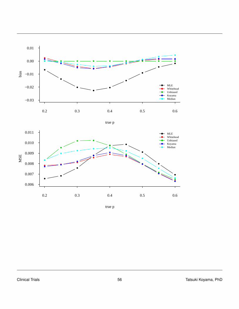
To compare these methods, we compute the bias of each estimator for various true values of p. Usebias and mean squared error = var + bias2 to compare them. For each estimator, compute p(X) forevery sample path (defined by X in [0,nt ]) and compute

Ep[p(X)] =nt

∑x=0

p(x)Pp[X = x].

Mean squared errors can be computed by

MSEp[p(X)] = Ep[(p(X)− p)2]

=nt

∑x=0

(p(x)− p)2Pp[X = x].

The following two plots show bias and MSE for the current example.


0.2 0.3 0.4 0.5 0.6

−0.03

−0.02

−0.01

0.00

0.01

true p

bias

●

●

●

●

●

●

●

●

●

●

●

●

●●

●

●● ●

● ● ● ● ● ● ● ● ●

●

●

●●

●

●

●● ●

●●

●

● ●

●

●

●●

●

●

●

●

●

MLEWhiteheadUnbiasedKoyamaMedian

0.2 0.3 0.4 0.5 0.6

0.006

0.007

0.008

0.009

0.010

0.011

true p

MS

E

●

●

●

●

●●

●

●

●

●●

●

●

●

●

●

●

●

●

●

● ●

●

●

●

●

●

●

●

●

●

●

●

●

●

●

●

●

●

●●

●

●

●

●

●

●

●

●

●

MLEWhiteheadUnbiasedKoyamaMedian


Chapter 6

Factorial design

6.1 Introduction

Factorial clinical trials (Piantadosi) Experiments that test the effect of more than one treatmentusing a design that permits an assessment of interactions among the treatments

The simplest example of a factorial design is 2 treatment, 2 treatment groups (2 by 2) designs. Withthis design, one group receives both treatment, a second group receives neither, and the other twogroups receive one of A or B.

Treatment BTreatment A No Yes Total

No n n 2nYes n n 2n

Total 2n 2n 4n

Four treatment groups and sample sizes in a 2×2 balanced factorial design.Alternatives to a 2×2 factorial design

• Two separate trials (for A and for B)

• Three arm trial (A, B, neither)

Two major advantages of factorial design (but not simultaneously):

• Allows investigation of interactions (drug synergy).

Drug synergy occurs when drugs interact in ways that enhance effects or side-effects of thosedrugs.

• Reduces the cost (sample size) if the drugs do not interact.


Some requirements for conducting a clinical trial with factorial design:

• The side effects of two drugs are not cumulative to make the combination unsafe to administer.

• The treatments need to be administered in combination without changing dosage of the indi-vidual drugs.

• It is ethical not to administer the individual drugs. A and B may be given in addition to a standarddrug so all groups receive some treatment.

• We need to be genuinely interested in studying drug combination, otherwise some treatmentcombinations are unnecessary.

Some terminology

• Factors (how many different treatments are in consideration)

• Levels (2 if yes/no)

• 2k factorial studies have k factors, each with two levels (presence/absence)

• Full factorial design has no empty cells.

• Unreplicated study has one sample per cell (obviously not very common in clinical studies)

• Fractional factorial designs (some cells are left empty by design)

• Complete block designs / Incomplete block designs

• Latin squares

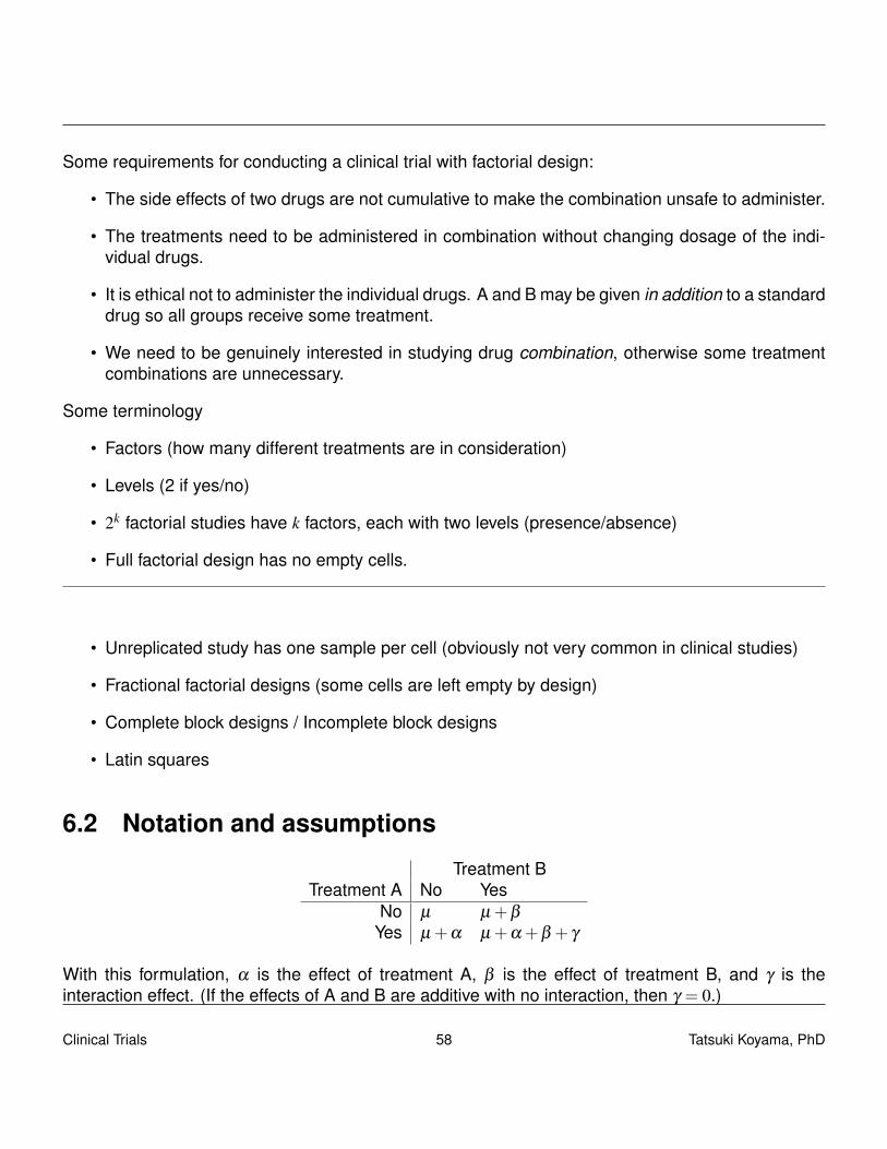
6.2 Notation and assumptions

Treatment BTreatment A No Yes

No µ µ +β

Yes µ +α µ +α +β + γ

With this formulation, α is the effect of treatment A, β is the effect of treatment B, and γ is theinteraction effect. (If the effects of A and B are additive with no interaction, then γ = 0.)


For a continuous outcome and large sample sizes (may be different for each group), we have thefollowing for the observed sample cell means.

Y 0 ∼ Normal(µ,σ2/n0)

Y A ∼ Normal(µ +α,σ2/nA)

Y B ∼ Normal(µ +β ,σ2/nB)

Y AB ∼ Normal(µ +α +β + γ,σ2/nAB)

We assume n = n0 = nA = nB = nAB.

6.3 Test for the interaction effect

In a factorial design, we usually test the presence of interaction effect first.

H0 : γ = 0H1 : γ 6= 0

The observed mean responses are:

Treatment B

Treatment A No Yes

No Y 0 Y B

Yes Y A Y AB

The interaction effect may be estimated by

γ = (YAB− YB)− (YA− Y0),

and

Var(γ) =4σ2

n. (Why is this problematic?)

Thus, if we assume σ2 is known, then

Z =γ

2σ/√

n

has Normal(0,1) distribution under H0.


If we have to estimate σ2 and assume within-group variances are equal, we use a pooled samplevariance, s2

p = (s20 + s2

A + s2B + s2

AB)/4.

The test statistic

t =γ

2sp/√

n

has a t distribution with d f = 4(n−1) under H0.

6.4 Treatemnt effect

6.4.1 γ 6= 0

The treatment A effect can be estimated as

α = YA− Y0,

and its variance is

Var(α) =2σ2

n.

And we have

Z =α√

2σ/√

n∼ Normal(0,1)

under H0. We can estimate σ2 by s2p = (s2

A + s20)/2. (Note: 2(n−1)s2

p/σ2 ∼ χ22(n−1).) Then

t =α√

2sp/√

n

has a t distribution with d f = 2(n−1) under H0. Constructing the test for β is exactly the same.


6.4.2 γ = 0

If no interaction is present then γ = 0, and α = YAB−YB can also be used to estimate α. If we use theaverage of α and α to estimate α, this estimator has a smaller variance.

α =α + α

2=

(YA− Y0)+(YAB− YB)

2

Var(α) =14

Var (YA− Y0 + YAB− YB) =σ2

n

Similarly to before,

Z =α

σ/√

n∼ Normal(0,1),and

t =α

sp/√

n∼ td f

under H0. (What’s the df?) Here we use

s2p = (s2

0 + s2A + s2

B + s2AB)/4,

and

4(n−1)σ2 s2

p ∼ χ24(n−1)

Constructing the test for β is exactly the same.In order to have the same efficiency in a two-arm trial (A vs placebo), we would need 2n patients ineach treatment arm.

var (α1) =2σ2

2n=

σ2

n.

So if we were to test A and B in two separate experiments we would need 2n per arm × 4 arms (Aand placebo, B and placebo), totaling 8n subjects. Noticing we are repeating the placebo in thesehypothetical experiments, we decide to use a 3-arm experiment with A, B, and placebo arms. Thenwe would require a total of 6n subjects for the same precision.

6.5 Examples

The group means are:



No 10 40Yes 30 60

If there is a synergistic effect, then η11 > 60.


No 10 40Yes 30 80


No 10 40Yes 30 120

In the last situation, the treatment effects may be multiplicative.


No log(10) = 1 log(40) = 1.60Yes log(30) = 1.48 log(120) = 2.08

Suppose the samples of size 20 yield the following estimates of the cell means.


No 9.83 40.05Yes 28.94 59.76

Assuming no interaction, to estimate the drug A effect we compute either

α1 = YA− Y0 = 28.94−9.83 = 19.11

or

α1 = YAB− YB = 59.76−40.05 = 19.71

or their average (19.11+19.71)/2 = 19.41.


How bad is it to estimate α1 this way when there is actually a significant interaction?

E[(α1 + α1)/2] =12

E[(YA− Y0)+(YAB− YB)]

=12((µ +α1)−µ +(µ +α1 +β1 + γ11)− (µ +β1))

= α1 +γ11

2

6.5.1 Example: the Physician’s Health Study I (1989)

Read all about it on http://phs.bwh.harvard.edu/.The Physician’s Health Study was a randomized clinical trial designed to test the following two theo-ries:

• Daily low-dose aspirin use reduces the risk of cardiovascular disease.

• Beta carotene reduces the risk of cancer.

Population hierarchy:

• 261,248 US male MDs aged 40 to 84.

• 112,528 responded to questionnaires.

• 59,285 willing to participate.

• 33,332 willing and eligible MDs enrolled in run-in (18 weeks of active aspirin and beta-caroteneplacebo).

Run-in period Eligible patients are monitored for treatment compliance.

• 22,071 randomized

Beta-caroteneAspirin Active Placebo TotalActive 5,517 5,520 11,037

Placebo 5,519 5,515 11,034Total 11,036 11,035 22,071

Major findings:

• The trial’s DSMB stopped the aspirin arm several years ahead of schedule on 1988/1/25 be-cause it was clear that aspirin had a significant effect on the risk of a first myocardial infarction.(It reduced the risk by 44%.)


– Did it change the sample sizes for the Beta-carotene components? (Next homework?)

• There were too few strokes or deaths to base sound clinical judgement regarding aspirin andstroke or mortality.

• The beta-carotene arm terminated as scheduled on 1995/12/12 with the conclusion that 13years of supplementation with beta-carotene produced neither benefit nor harm. Beta-carotenealone was not responsible for the health benefit seen among people who ate plenty of fruits andvegetables.

• Over 300 other findings have emerged from the trial so far.

6.6 Treatment interactions

Factorial designs are the only way to study treatment interactions. Recall the interaction term isestimated by γ = (YAB−YB)− (YA−Y0), and its variance is Var(γ) = 4σ2/n. This variance is 2 times aslarge as that of A and B main effects, and to have the same precision for an estimate of an interactioneffect, the sample size has to be 4 times as large. This means, the two main advantages of thefactorial designs (efficiency and interaction objectives) cannot be satisfied simultaneously.When there is an AB interaction, we cannot use the estimators, α and β , which are only valid with nointeraction effect. In fact, we cannot talk about an overall main effect in the presence of an interaction.Instead, we can talk about the effect of A in the absence of B,

α = YA− Y0,

or the effect of A in the presence of B

α′ = α + γ = YAB− YB.

Some additional notes

• In the 2× 2× 2 design (23 design), there are 3 main effects and 4 interactions possible. Thenumber of high order interactions will grow quickly with k, but oftentimes, they are (assumed tobe) 0.

• A “quantitative” interaction does not affect the direction of the treatment effect. For examplewhen treatment B is effective either with or without treatment A, but the magnitude of its effec-tiveness changes.

• With a “qualitative” interaction, the effects of A are reversed with the presence of B. In this case,an overall treatment A effect does not make sense.


• The factorial design can be analyzed with linear models (analysis of variance models).

Limitations of factorial designs

• A higher level design can get complex quickly.

• Test for interaction requires a large sample size (or have a very low power if the study is pow-ered for the main effects).

• Combination therapy may be considered as a treatment in its own right.

Of further interest...

• Partial (fractional) factorial designs have missing cells by design (especially when higher orderinteractions are assumed to be zero)


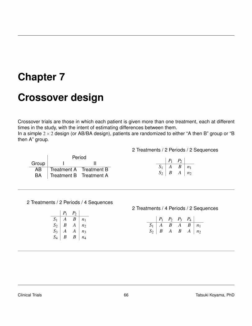
Chapter 7

Crossover design

Crossover trials are those in which each patient is given more than one treatment, each at differenttimes in the study, with the intent of estimating differences between them.In a simple 2×2 design (or AB/BA design), patients are randomized to either “A then B” group or “Bthen A” group.

PeriodGroup I II

AB Treatment A Treatment BBA Treatment B Treatment A

2 Treatments / 2 Periods / 2 Sequences

P1 P2S1 A B n1S2 B A n2


P1 P2S1 A B n1S2 B A n2S3 A A n3S4 B B n4


P1 P2 P3 P4S1 A B A B n1S2 B A B A n2


7.1 Some characteristics of crossover design

• All subjects receive more than one treatment (not simultaneously).

• Each subject acts as own control. Therefore, the treatment groups are comparable withoutrelying on randomization.

– Treatment periods (order of A and B) are often randomly assigned.

– Baseline characteristics are identical with regard to many patient characteristics, but notwith regard to their recent history of exposure to other potentially effective treatments.carryover effects

– The comparability of the treatment groups is not guaranteed by the structure of the trialalone. The investigators need to estimate the carryover effects.

• Crossover designs are not used ...

– with any condition that treatment could effect considerable change.

– for acute illness.

• Crossover designs are most suitable for treatments intended for rapid relief of symptoms inchronic diseases, where the long-term condition of the patient remains fairly stable.

PrecisionThe primary strength of crossover trials is increased efficiency. Suppose the treatment effects are

Yt ∼ Normal(µt ,σ2),

Yc ∼ Normal(µc,σ2),

and we are interested in µt−µc. In a parallel design (with per group sample size of n), we have

∆ = Y t−Y c ∼ Normal(

µt−µc,2σ2

n

).

With a TC/CT crossover design with sample size of n,

var(∆) =2σ2

n−2cov(Y t ,Y c)

=2σ2

n(1−ρtc) ,

where ρtc is the within-subject correlation of responses on treatments T and C. Therefore, a crossoverdesign is more efficient than a parallel design given ρtc > 0.


RecruitmentSome patients may hesitate to participate in a clinical trial if there is a 50% probability of not receivingany effective treatment. With a crossover design, everyone is guaranteed to receive the test drug.On the other hand, the patients may hesitate to participate in a crossover trial because they will gothrough more than one treatment, especially when outcomes are assessed with diagnostic proce-dures such as X-ray, blood drawing, lengthy questionnaires.Carryover effectsThe biggest concern is the possibility that the treatment effect from one period might continue tobe present during the following period. A sufficiently long “washout” period between the treatmentsmay prevent significant carryover effects (but how long is sufficiently long?). If there are baselinemeasurements that represent patient’s disease status, this can be checked against their baselinelevels.If the treatment effects a permanent change or cure in the underlying condition, the treatment givenafter could look artificially superior.DropoutsIn a crossover design, the trial duration tends to be longer than a comparable study using inde-pendent groups, which may cause more dropouts. Also because every patient take more than onetreatment, dropouts due to severe side effects may also increase. The consequences of dropoutsare more severe in crossover trial; a simple analysis cannot use only the data from the first period.

7.2 Analysis of 2×2 crossover design

P1 P2

S1 = AB µA1 = β0 µB2 = β0 +β1 +β2

S2 = BA µB1 = β0 +β1 µA2 = β0 +β2 +β3

β0 · · · Treatment A effectβ1 · · · Increment of treatment effect due to B.β2 · · · Carryover effect of treatment Aβ3 · · · Increment carryover effect of treatment BTreatment B effect is β0 +β1, and the carryover effect due to treatment B is β2 +β3.The primary hypotheses to test are:

H0 : β1 = 0H1 : β1 6= 0

And how to conduct this test (how to estimate β1) depends on whether β3 = 0. (We’ll see why later.)Step 0: Assumptions


1. Sample size is n for S1 and S2.

2. Y ∼ Normal(µ,σ2/n

).

3. Cor(YA1,YB2) =Cor(YB1,YA2) = ρ.

Data:

P1 P2

S1 = AB Y A1 = β0 Y B2 = β0 + β1 + β2

S2 = BA Y B1 = β0 + β1 Y A2 = β0 + β2 + β3

Step 1: Test β3 = 0Note that under H0 : β3 = 0, we have µA1 +µB2 = µB1 +µA2. Thus, we can use

Z1 =(Y B1 +Y A2)− (Y A1 +Y B2)√

Var(Y B1 +Y A2)+Var(Y A1 +Y B2)

to test these hypotheses (assuming σ2 is known).

Why is this good (convenient)? Because we don’t have to worry about the correlations when com-puting Z1. Instead, we can compute the within-subject difference sum. Let’s say ωi1 = yA1i + yB2i andω j2 = yB1 j + yA2 j. Then we have

Z1 =ω2−ω1√

Var(ω2)+Var(ω1)

If we don’t assume σ2 is known, we can use a simple two-sample t-test.

t1 =ω2−ω1√2sω/

√n,

where s2ω = (s2

ω1+ s2

ω2)/2. What’s the degree of freedom?

Why is this bad?


Step 2a (If β3 = 0)

We can estimate β1 and test if H0 : β1 = 0. Let’s say δi1 = yB2i−yA1i and δ j2 = yA2 j−yB1 j. Let’s confirmthat the following test statistic can be used to test this hypothesis.

t2 =δ 1−δ 2√2sδ/√

n,

where s2δ= (s2

δ1+ s2

δ2)/2. What’s the degree of freedom?

We are interested in estimating β1. Note that β1 = (δ 1−δ 2)/2. So a 95% confidence interval for β1 is

β1± t0.975,2(n−1)se(β1)

δ 1−δ 2

2± t0.975,2(n−1)

√s2

δ/(2n)

Step 2b (If β3 = 0)

We can estimate β2 and test if H0 : β2 = 0. Note that β2 = (δ 1+δ 2)/2 and se(β2) = se(β1). Thus a 95%confidence interval for β2 is

δ 1 +δ 2

2± t0.975,2(n−1)

√s2

δ/(2n)

But we are not that interested in estimating β2.

Step 2c (If β3 = 0)

Maybe we want to estimate β0. We have two estimates of β0, and we can take the average of themto get

β0 =12(Y A1 +(Y B1 +Y A2−Y B2)

)=

12(Y B1 +Y A2− (Y B2−Y A1)

)=

12(ω2−δ 1)


This means we can test to see if β0 = 0 by testing

H0 : µB1 +µA2 = µB2−µA1

H1 : µB1 +µA2 6= µB2−µA1

Constructing the relevant t test statistic is not as straightforward as the previous steps because wecannot assume the true variances of ω2 and δ1 are equal. We can use

t =ω2−δ 1√

s2ω2n +

s2δ1n

,

which follows a t distribution approximately with estimated degrees of freedom given by the Satterth-waite formula.To estimate β0 with a confidence interval, compute a confidence interval

(ω2−δ 1)± t1−α/2,d f

√s2

ω2

n+

s2δ1

n

first (applying the unequal-varince t-test), and divide it by 2.

Step 2d (If β3 = 0)

Maybe we want to estimate β0 +β1. Again we can use the average of two estimates:

β0 + β1 =12(Y B1 +(Y B2−Y A2 +Y A1)

)=

12(Y A1 +Y B2− (Y A2−Y B1)

)=

12

(ω1−δ 2

)Follow the same process as in step 2c.

Step 3 (If β3 6= 0)

Because the carryover affects S1 and S2 differently, we cannot eliminate β2 as we did before.

Y B2−Y A1 = β1 + β2

Y B1−Y A2 = β1− β2− β3


Taking the within-individual difference is not going to help, so we cannot take an advantage of thecorrelated endpoint. In this case, we ignore the data from the second period.

β1 = Y B1−Y A1

Var(β1) =2σ2

n

Treat the study as a two sample test with sample size = n per group.

Moreover, we can estimate the treatment effects with

β0 = Y A1

β0 + β1 = Y B1

7.2.1 Variance of β

Step 1

β3 = (Y A2−Y A1)− (Y B2−Y B1)

Var(β3) =4σ2

n(1+ρ)


Step 2 (If β3 = 0)

β1 =12((Y B2−Y A1)+(Y B1−Y A2)

)Var(β1) =

σ2

n(1−ρ)

β2 =12((Y B2−Y A1)− (Y B1−Y A2)

)Var(β2) =

σ2

n(1−ρ)

β0 =12((Y A1−Y B2)+(Y B1 +Y A2)

)Var(β0) =

σ2

n

β0 + β1 =12((Y B1−Y A2)+(Y A1 +Y B2)

)Var(β0 + β1) =

σ2

n

Step 3 (If β3 6= 0)

β1 = Y B1−Y A1

Var(β1) =2σ2

nβ0 = Y A1

Var(β0) =σ2

nβ0 + β1 = Y B1

Var(β0 + β1) =σ2

n

In step 2 and 3, variances of β0 and β0 + β1 are the same.Var{β3} is at least twice as large as Var{β2} for ρ ≥ 0. Therefore, any crossover trial designed todetect the differential treatment effects will have lower power for difference of the carryover effects,which is critical to detect the subsequent analysis and interpretation of the trial will be different.With the presence of a clinically important carryover effect difference, a crossover design is no moreefficient than an independent-groups trial.A two-stage procedure may be used: the difference of carryover effects is tested first with a type I


error rate of 10 ∼ 20% before moving on to the primary hypothesis testing of the treatment effects.Estimates will be different depending on the conclusion from the first stage.

7.3 Examples

7.3.1 From clinicalTrials.gov

Capecitabine/Erlotinib Followed of Gemcitabine Versus Gemcitabine/Erlotinib Followed ofCapecitabinehttp://clinicaltrials.gov/ct2/show/NCT00440167This crossover trial is performed in advanced and metastatic pancreatic cancer not previously ex-posed to chemotherapy. The study compares a standard arm with gemcitabine plus erlotinib toan experimental arm with capecitabine plus erlotinib. It is the first trial of its kind to incorporatesecond-line treatment into the study design. Patient who fail on first-line therapy are switched tothe comparator chemotherapy without erlotinib. The trial therefore not only compares two differentregimens of first-line treatment, it also compares two sequential treatment strategies.

Colchicine Randomized Double-Blind Controlled Crossover Study in Behcet’s Diseasehttp://clinicaltrials.gov/ct2/show/study/NCT00700297Method: patients were randomized at the study entry to take either colchicine or placebo. At 4months, they were crossed over. Those who were taking colchicine went on placebo and those onplacebo went on colchicine. Each patient tried therefore, both colchicine and placebo. The primaryoutcome was the effect of colchicine on the disease activity index, the IBDDAM (16-17). To calcu-late the overall IBDDAM of the baseline, the IBDDAM of the last 12 months (prior to the study) ofeach manifestation was calculated and added together. The overall disease activity index was thendivided to the number of months (12 months) to have the mean activity index per month. IBDDAMwas then measured every 2 months (in the middle and at the end, in each arm of the study). Thetotal IBDDAM of the 4 months was then divided by 4 to have the mean activity index per month. Thesecondary outcome was to see how the individual symptoms responded to colchicine (IBDDAM ofeach manifestation).

Statistical analysis: The analysis was done by the intention to treat method. As the difference be-tween IBDDAM before and after treatment had normal distribution Student T test for paired sampleswere used to evaluate the outcome in the colchicine and the placebo group. As the Levene’s testshowed the homogeneity of variance, ANOVA (one way) was used to test the effect of treatment(colchicine and placebo) and gender on patients’ outcome. The dependent variable was the dif-ference between IBDDAM (before and after the treatment). The independent variables were thetreatment, and the gender. SPSS 15 was used for all statistical calculations.


A Placebo-Controlled, Cross-Over Trial of Aripiprazolehttp://clinicaltrials.gov/ct2/show/record/NCT00351936Primary endpoint: Evaluate the effects of aripiprazole on weight, Body Mass Index (BMI), andwaist/hip circumference.This study is a ten-week, placebo-controlled, double-blind, cross-over, randomized trial of the novelantipsychotic agent, aripiprazole, added to 20 obese stable olanzapine-treated patients with schizophre-nia or schizoaffective disorder. The advantage of the crossover design is that each subject will actas their own control and fewer subjects will be required.

The double-blind, placebo-controlled, crossover study will consist of two random order 4-week treat-ment arms (aripiprazole 15 mg or placebo) separated by a 2-week adjuvant treatment washout.Following baseline, subjects will be randomized, double-blind, to either aripiprazole or placebo for 4weeks. After the initial 4 weeks of medication patients will be reassessed, have a 2-week washoutperiod and then crossover to the other treatment for another 4 weeks.

Data management and statistical analysis will be provided by Dr. David Schoenfeld from the Mas-sachusetts General Hospital, Biostatistics Center.

7.4 Examples

7.4.1 Hills and Armitage

Hills M, Armitage P (1979) “The two-period cross-over clinical trial”. Br J Clin Pharmacol. 8: 7-20.

• Children with enuresis were treated with a new drug or placebo for 14 days

• The primary data are number of dry nights out of 14.

An estimate of within-subject differences (treatment effects) is δ =YA−YB. The carryover effects maybe estimated by

Z1 =δ 1−δ 2√

var(δ 1)+ var(δ 2),

and Z is approximately normally distributed under H0. Similarly the overall treatment effect can beestimated by

Z2 =δ 1 +δ 2√

var(δ 1)+ var(δ 2),


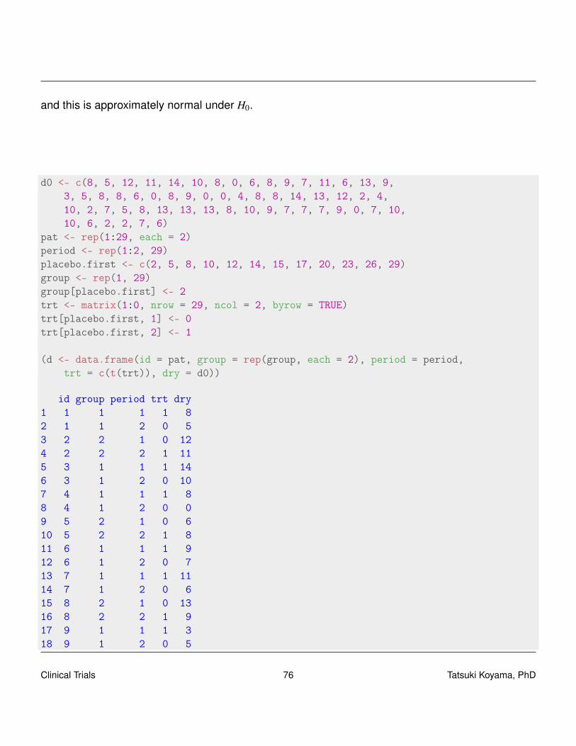
and this is approximately normal under H0.

d0 <- c(8, 5, 12, 11, 14, 10, 8, 0, 6, 8, 9, 7, 11, 6, 13, 9,3, 5, 8, 8, 6, 0, 8, 9, 0, 0, 4, 8, 8, 14, 13, 12, 2, 4,10, 2, 7, 5, 8, 13, 13, 13, 8, 10, 9, 7, 7, 7, 9, 0, 7, 10,10, 6, 2, 2, 7, 6)

pat <- rep(1:29, each = 2)period <- rep(1:2, 29)placebo.first <- c(2, 5, 8, 10, 12, 14, 15, 17, 20, 23, 26, 29)group <- rep(1, 29)group[placebo.first] <- 2trt <- matrix(1:0, nrow = 29, ncol = 2, byrow = TRUE)trt[placebo.first, 1] <- 0trt[placebo.first, 2] <- 1

(d <- data.frame(id = pat, group = rep(group, each = 2), period = period,trt = c(t(trt)), dry = d0))

id group period trt dry1 1 1 1 1 82 1 1 2 0 53 2 2 1 0 124 2 2 2 1 115 3 1 1 1 146 3 1 2 0 107 4 1 1 1 88 4 1 2 0 09 5 2 1 0 610 5 2 2 1 811 6 1 1 1 912 6 1 2 0 713 7 1 1 1 1114 7 1 2 0 615 8 2 1 0 1316 8 2 2 1 917 9 1 1 1 318 9 1 2 0 5


19 10 2 1 0 820 10 2 2 1 821 11 1 1 1 622 11 1 2 0 023 12 2 1 0 824 12 2 2 1 925 13 1 1 1 026 13 1 2 0 027 14 2 1 0 428 14 2 2 1 829 15 2 1 0 830 15 2 2 1 1431 16 1 1 1 1332 16 1 2 0 1233 17 2 1 0 234 17 2 2 1 435 18 1 1 1 1036 18 1 2 0 237 19 1 1 1 738 19 1 2 0 539 20 2 1 0 840 20 2 2 1 1341 21 1 1 1 1342 21 1 2 0 1343 22 1 1 1 844 22 1 2 0 1045 23 2 1 0 946 23 2 2 1 747 24 1 1 1 748 24 1 2 0 749 25 1 1 1 950 25 1 2 0 051 26 2 1 0 752 26 2 2 1 1053 27 1 1 1 1054 27 1 2 0 655 28 1 1 1 256 28 1 2 0 257 29 2 1 0 758 29 2 2 1 6


# Group 1: trt -> placebog1 <- subset(d, group == 1)g2 <- subset(d, group == 2)

ms <- function(v) c(mean(v), sd(v)/sqrt(length(v)))

g1.diff <- matrix(g1$dry, ncol = 2, byrow = TRUE)ms(g1.diff[, 1] - g1.diff[, 2])

[1] 2.824 0.841

g2.diff <- matrix(g2$dry, ncol = 2, byrow = TRUE)ms(g2.diff[, 2] - g2.diff[, 1])

[1] 1.250 0.863

z1 =2.82−1.25√

0.84122 +0.86272= 1.30

z2 =2.82+1.25√

0.84122 +0.86272= 3.38

7.5 A two-period crossover design for the comparison of twoactive treatments and placebo

By GG Koch, IA Amara, BW Brown, T Colton, and DB Gillings (1989).

Consider sequences of treatments TT, TC, and CT.

1. The first period is parallel group design to address direct use in all patients

2. The second period for TT versus TC is a parallel group comparison design to address T versusC for patients who received T during the first period.

3. The second period for TT versus CT enables “delayed start” assessment of T relative to C ifdropout during the first period is minimal and non-informative.

4. The second period for CT versus TC is for assessment of T relative C if carryover effects aresmall.


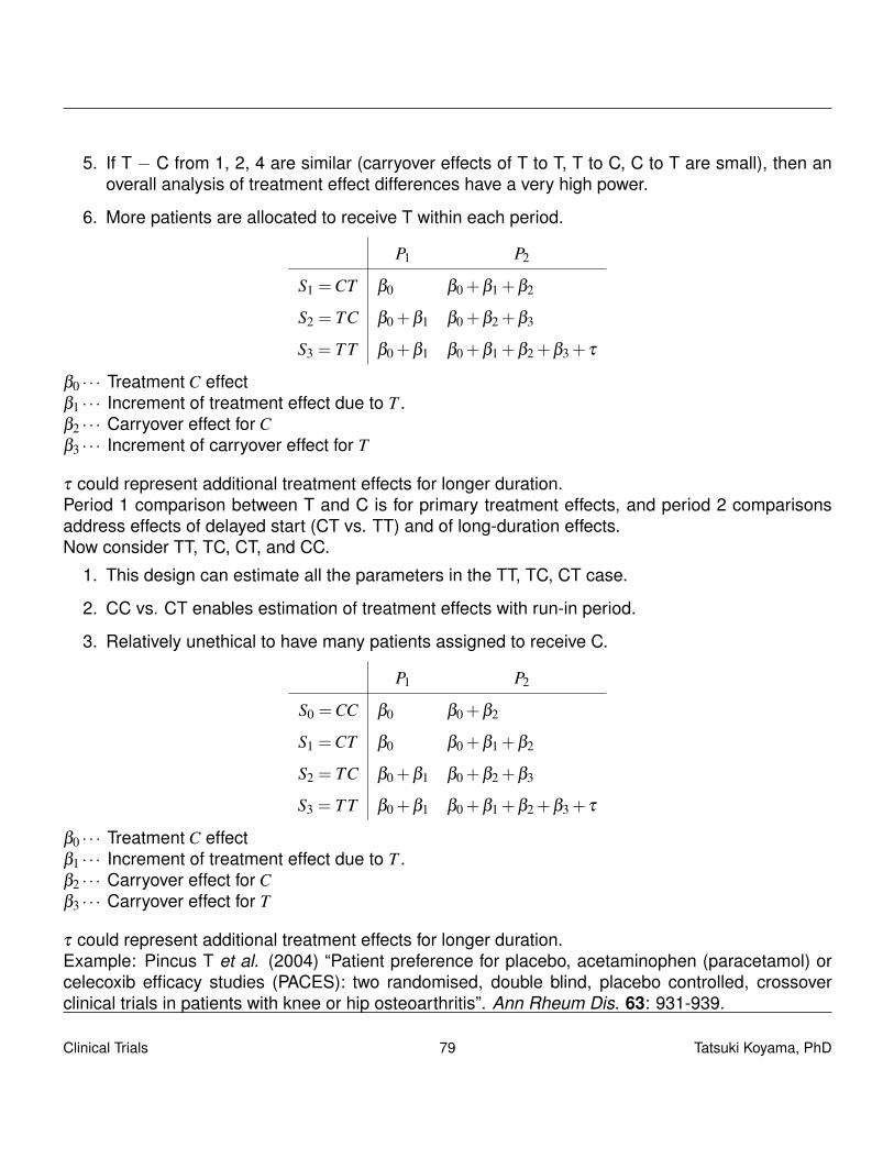
5. If T − C from 1, 2, 4 are similar (carryover effects of T to T, T to C, C to T are small), then anoverall analysis of treatment effect differences have a very high power.

6. More patients are allocated to receive T within each period.

P1 P2

S1 =CT β0 β0 +β1 +β2

S2 = TC β0 +β1 β0 +β2 +β3

S3 = T T β0 +β1 β0 +β1 +β2 +β3 + τ

β0 · · · Treatment C effectβ1 · · · Increment of treatment effect due to T .β2 · · · Carryover effect for Cβ3 · · · Increment of carryover effect for T

τ could represent additional treatment effects for longer duration.Period 1 comparison between T and C is for primary treatment effects, and period 2 comparisonsaddress effects of delayed start (CT vs. TT) and of long-duration effects.Now consider TT, TC, CT, and CC.

1. This design can estimate all the parameters in the TT, TC, CT case.

2. CC vs. CT enables estimation of treatment effects with run-in period.

3. Relatively unethical to have many patients assigned to receive C.

P1 P2

S0 =CC β0 β0 +β2

S1 =CT β0 β0 +β1 +β2

S2 = TC β0 +β1 β0 +β2 +β3

S3 = T T β0 +β1 β0 +β1 +β2 +β3 + τ

β0 · · · Treatment C effectβ1 · · · Increment of treatment effect due to T .β2 · · · Carryover effect for Cβ3 · · · Carryover effect for T

τ could represent additional treatment effects for longer duration.Example: Pincus T et al. (2004) “Patient preference for placebo, acetaminophen (paracetamol) orcelecoxib efficacy studies (PACES): two randomised, double blind, placebo controlled, crossoverclinical trials in patients with knee or hip osteoarthritis”. Ann Rheum Dis. 63: 931-939.


7.6 Latin squares

When there are k treatments and each patient is to receive all k treatments. Then there are k!possible sequences. Three treatments yield 6 sequences, four treatments yield 24, and five yield120.k = 3: ABC, ACB, BAC, BCA, CAB, CBAThe idea is to use a reduced number of sequences (reduced sample size) but maintain a good“representation”, i.e., every treatment is represented in every period with the same frequency.

P1 P2 P3S1 A B CS2 B C AS3 C A B

P1 P2 P3S1 A C BS2 B A CS3 C B A

There are 6!/(3!)(3!) = 20 ways to choose 3 sequences from 6, but only 2 of those are Latin squares.

7.7 Optimal designs

There is an extensive literature on optimal choice of sequences for measuring treatment effects inthe presence of carryover.

• More advanced theory · · ·

• Optimality depends on assumptions about carryover effects

Concerns about carryover can be reduced by using designs with more than two periods. (Laska E,Meisner M, Kushner HB. (1983) “Optimal crossover designs in the presence of carryover effects”.Biometrics. 39(4): 1087-1091.Consider treatments A and B in two sequences: AABB and BBAA. This design is not uniquely optimal,but it can be used to estimate treatment effects with more efficiency than using data from period 1.

P1 P2 P3 P4AABB µ11 = µ +π1 + τa µ12 = µ +π2 + τa +λa µ13 = µ +π3 + τb +λa µ14 = µ +π4 + τb +λbBBAA µ21 = µ +π1 + τb µ22 = µ +π2 + τb +λb µ23 = µ +π3 + τa +λb µ24 = µ +π4 + τa +λa

Note µ is the overall mean, π is the period effect, τ is the treatment effect, and λ is the carryovereffect.To obtain an unadjusted (for carryover effect) treatment effect (B−A), use the following weights.

P1 P2 P3 P4AABB −1/4 −1/4 1/4 1/4BBAA 1/4 1/4 −1/4 −1/4

• Weights sum to 1 for B and −1 for A to form a contrast B−A.


• Weights sum to 0 over sequence and period.

− 14

µ11−14

µ12 +14

µ13 +14

µ14 +14

µ21 +14

µ22−14

µ23−14

µ24

= (τb− τa)+(λb−λa)/4

When carryover effects are present, we can construct weights so that carryover effects will be elimi-nated.

P1 P2 P3 P4AABB −w1 −w2 w3 w4BBAA w1 w2 −w3 −w4

Constraints on w’s.

• w1 +w2 +w3 +w4 = 1

• w2−w3 +w4 = 0

−w1µ11−w2µ12 +w3µ13 +w4µ14 +w1µ21 +w2µ22−w3µ23−w4µ24

=−w1τa−w2(τa +λa)+w3(τb +λa)+w4(τb +λb)+w1τb +w2(τb +λb)−w3(τa +λb)−w4(τa +λa)

= (w1 +w2 +w3 +w4)τb− (w1 +w2 +w3 +w4)τa− (w2−w3 +w4)λa +(w2−w3 +w4)λb

= τb− τa

Let σ2 be the within-patient variance and n be the number of patients per sequence. The variance ofthe unadjusted estimator is

2

{(14

)2

+

(14

)2

+

(14

)2

+

(14

)2}

σ2

n= 0.5

σ2

n.

And for adjusted estimator:

2{

w21 +w2

2 +w23 +w2

4} σ2

n.

If we pick w1 = 4/10, w2 = 2/10, w3 = 3/10, w4 = 1/10, we have

2

{(4

10

)2

+

(2

10

)2

+

(310

)2

+

(1

10

)2}

σ2

n= 0.6

σ2

n.


If we only use data from the first period

2{

12 +02 +02 +02} σ2

n= 2

σ2

n.

The adjusted estimator has slightly higher variance, but it is unbiased with presence of carryover.William’s squareWhen an even number of treatments are considered in the same number of periods, William’s squaregives an optimal design. (Williams EJ (1949). “Experimental designs balanced for the estimation ofresidual effects of treatments”. Australian Journal of Scientific Research. Series A2. 149-168.) It isa Latin square design in which every treatment precedes every other treatments exactly once.

P1 P2 P3 P4sequence 1 A B C Dsequence 2 B D A Csequence 3 C A D Bsequence 4 D C B A

Latin square designs are a special type of incomplete block design.Example:An experiment was conducted to study the effects of different types of background music on theproductivity (Y ) of bank tellers. The treatments were defined as five combinations of temp and styleof music:A: slow, instrumental and vocalB: medium, instrumental and vocalC: fast, instrumental and vocalD: medium, instrumental onlyE: fast, instrumental onlyThere are 120 possible sequences of these treatments.


Chapter 8

Group sequential design

8.1 Introduction

Fully sequential method A test of significance is repeated after each observation.

Group sequential method A test of significance is repeated after a group of observations.

Some basic characteristics of a group sequential method

• The response variable needs to be observed immediately.

• Number of stages (or looks) can be 2 to 20.

• Looks are equally spaced. (This is not a critical requirement.)

• At each interim (and final) analysis, compute summary statistic based on the cumulative data.

• A group sequential method is a strategy to stop early as opposed to an “adaptive design”, whichis often viewed as a strategy to extend the study if necessary.

• A set of critical values are computed so that the overall α is as specified.

– Haybittle-Peto (1971)This is an ad hoc method in which a very conservative critical value (e.g., Z > 3) is usedat every interim test. At the final analysis, no adjustment is used (i.e., Z >−1.960)It is highly unlikely to stop early.

– Pocock (1977)A ”repeated test of significance” at a constant significance level to analyze accumulatingdata.

– O’Brien-Fleming (1979)The significance levels increase as the study progress.


8.2 Example

For testing

µt−µc = 0µt−µc > 0

With α = 0.025 and power= 0.90 at δ1 = 0.25 (σ2 = 1), 5-stage group-sequential designs are:

library(gsDesign)

x.of <- gsDesign(k = 5, test.type = 2, alpha = 0.025, beta = 0.1,delta0 = 0, delta1 = 0.25, n.fix = 1, sfu = "OF")

x.po <- gsDesign(k = 5, test.type = 2, alpha = 0.025, beta = 0.1,delta0 = 0, delta1 = 0.25, n.fix = 1, sfu = "Pocock")


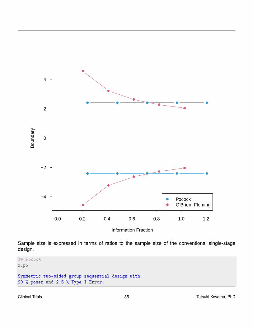
0.0 0.2 0.4 0.6 0.8 1.0 1.2

−4

−2

0

2

4

Information Fraction

Bou

ndar

y

PocockO'Brien−Fleming

Sample size is expressed in terms of ratios to the sample size of the conventional single-stagedesign.

## Pocockx.po

Symmetric two-sided group sequential design with90 % power and 2.5 % Type I Error.


Spending computations assume trial stopsif a bound is crossed.

SampleSize

Analysis Ratio* Z Nominal p Spend1 0.241 2.41 0.0079 0.00792 0.483 2.41 0.0079 0.00593 0.724 2.41 0.0079 0.00454 0.965 2.41 0.0079 0.00375 1.207 2.41 0.0079 0.0031

Total 0.0250

++ alpha spending:Pocock boundary.

* Sample size ratio compared to fixed design with no interim

Boundary crossing probabilities and expected sample sizeassume any cross stops the trial

Upper boundary (power or Type I Error)Analysis

Theta 1 2 3 4 5 Total E{N}0.00 0.0079 0.0059 0.0045 0.0037 0.0031 0.025 1.1773.24 0.2059 0.2603 0.2086 0.1402 0.0851 0.900 0.685

Lower boundary (futility or Type II Error)Analysis

Theta 1 2 3 4 5 Total0.00 0.0079 0.0059 0.0045 0.0037 0.0031 0.0253.24 0.0000 0.0000 0.0000 0.0000 0.0000 0.000

## O'Brien-Flemingx.of

Symmetric two-sided group sequential design with90 % power and 2.5 % Type I Error.Spending computations assume trial stopsif a bound is crossed.

Sample


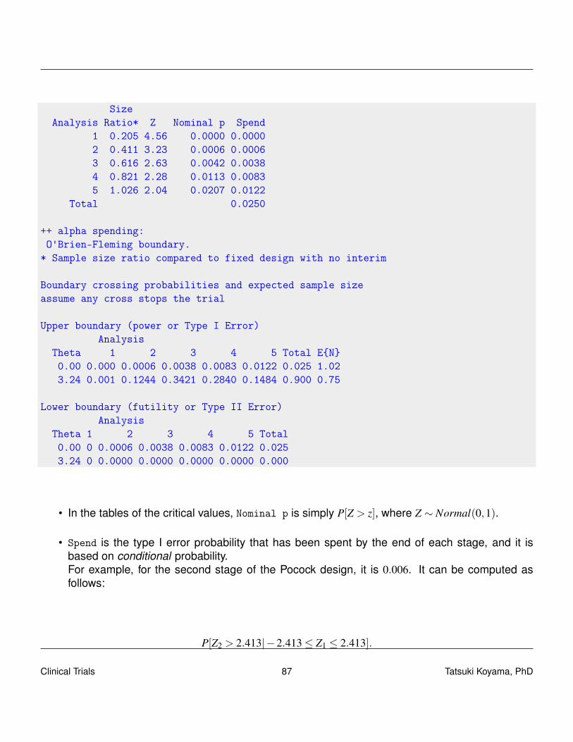
SizeAnalysis Ratio* Z Nominal p Spend

1 0.205 4.56 0.0000 0.00002 0.411 3.23 0.0006 0.00063 0.616 2.63 0.0042 0.00384 0.821 2.28 0.0113 0.00835 1.026 2.04 0.0207 0.0122

Total 0.0250

++ alpha spending:O'Brien-Fleming boundary.




Theta 1 2 3 4 5 Total E{N}0.00 0.000 0.0006 0.0038 0.0083 0.0122 0.025 1.023.24 0.001 0.1244 0.3421 0.2840 0.1484 0.900 0.75


Theta 1 2 3 4 5 Total0.00 0 0.0006 0.0038 0.0083 0.0122 0.0253.24 0 0.0000 0.0000 0.0000 0.0000 0.000

• In the tables of the critical values, Nominal p is simply P[Z > z], where Z ∼ Normal(0,1).

• Spend is the type I error probability that has been spent by the end of each stage, and it isbased on conditional probability.For example, for the second stage of the Pocock design, it is 0.006. It can be computed asfollows:

P[Z2 > 2.413|−2.413≤ Z1 ≤ 2.413].


8.3 General applications

Let k = 1, · · · ,K be denote the stages so that we have

X (k)t − X (k)

c =1

ntk

ntk

∑i=1

Xti−1

nck

nck

∑i=1

Xci

∼ Normal(

µt−µc,σ2

ntk+

σ2

nck

),

where ntk and nck are the cumulative sample sizes for the treatment and control groups. Note thatthis is not a conditional distribution but a marginal distribution.

Define “information” as Ik = (σ2/ntk +σ2/nck)−1. Roughly speaking, information is square of what

appears in the denominator of the test statistic, Z. When nk = ntk = nck, Ik = (2σ2/nk)−1.

The test statistic for stage k is

Zk =X (k)

t − X (k)c√

2σ2/nk= (X (k)

t − X (k)c )√

Ik.

The vector, (Z1, · · · ,Zk), has a multivariate normal distribution because each Zk is a linear combinationof the independent normal variates Xti and Xci. The marginal distribution of Zk is

Zk ∼ Normal((µt−µc)

√Ik,1

).


How about the covariance of Zk1 and Zk2 for k1 < k2?

Cov(Zk1,Zk2) =Cov({X (k1)

t − X (k1)c }

√Ik1, {X

(k2)t − X (k2)

c }√

Ik2

)=Cov

({X (k1)

t − X (k1)c }, {X (k2)

t − X (k2)c }

)√Ik1

√Ik2

=[Cov

(X (k1)

t , X (k2)t

)+Cov

(X (k1)

c , X (k2)c

)]√Ik1

√Ik2

Cov(

X (k1)t , X (k2)

t

)=Cov

(1

nk1

nk1

∑i=1

Xi,1

nk2

nk1

∑i=1

Xi +1

nk2∑Xi

)

=1

nk1

1nk2

Var

(nk1

∑i=1

Xi

)=

1nk2

σ2

Cov(Zk1,Zk2) = σ2(

1nk2

+1

nk2

)√Ik1

√Ik2

=√

Ik1/Ik2.

Therefore,

• (Z1, · · · ,ZK) is multivariate normal.

• E[Zk] = (µt−µc)√

Ik, k = 1, · · · ,K, and

• Cov(Zk1,Zk2) =√

Ik1/Ik2, 1≤ k1 ≤ k2 ≤ K.

General decision rule for a group sequential design isAfter group k = 1, · · · ,K−1

if |Zk| ≥ ck stop and reject H0.otherwise continue to group k+1.

After group Kif |Zk| ≥ cK stop and reject H0.otherwise stop for futility.

The test’s type I error rate can be expressed as

P{|Zk| ≥ ck for some k = 1, · · · ,K} .

The critical values, ck, are chosen so that the above probability is equal to α. And the power of thestudy at δ1 is

P

{K⋃

k=1

(|Z j|< c j, for j = 1, · · · ,k−1 and |Zk| ≥ ck

)}.


Evaluation of this probability requires knowing the distribution of (Z1, · · · ,ZK). Refer to tables of cKvalues or a computer software.

• For a Pocock method, the critical values are constant, so ck = CP(K,α). That is, specifying α

and K uniquely determines the critical values.

• For the previous example, CP(5, 0.025) = 2.413.

• For an O’Brien-Fleming method, the critical values have the form, ck =CB(K,α)√

K/k

• For the same example, CB(5, 0.025) = 2.040. And the other critical values are: 2.040√

5/4,2.040

√5/3, and so on.

(K.of)

[1] 2.04

K.of * sqrt(5/(5:1))

[1] 2.04 2.28 2.63 3.23 4.56

• More generally, if stage sample sizes are different, use Ik, that is, ck =CB(K,α)√

IK/Ik.

8.3.1 Beta blocker heart attack trial

Seven analyses (including the final one) were planned (corresponding to the timing of the DataMonitoring Committee meetings) using O’Brien-Fleming bounds with two-sided type I error rate of5%. The primary outcome was survival, and log-rank test was used.


If Pocock boundary had been used, N = 7 and α = 0.05 give Z = 2.485. Therefore, the trial wouldhave been stopped at the same point.

8.3.2 non-Hodgkin’s lymphoma

Pocock 1983 Clinical Trials: A Practical Approach. A trial was conducted in patients with non-Hodgkin’s lymphoma for two drug combinations (cytoxanprednisone -CP- and cytoxan-vincristine-prednisone -CVP-). The primary endpoint was tumor shrinkage (Yes/No).Statistical analyses were planned after approximately 25 patients. With 5 looks and one-sided α =0.05. The Pocock procedure requires a significance level of 0.017 at each analysis. χ2 tests withoutthe continuity correction were performed at each of the 5 scheduled analyses.

gsDesign(k = 5, test.type = 1, alpha = 0.05, n.fix = 1, sfu = "Pocock")

One-sided group sequential design with90 % power and 5 % Type I Error.

SampleSize

Analysis Ratio* Z Nominal p Spend1 0.246 2.12 0.0169 0.0169


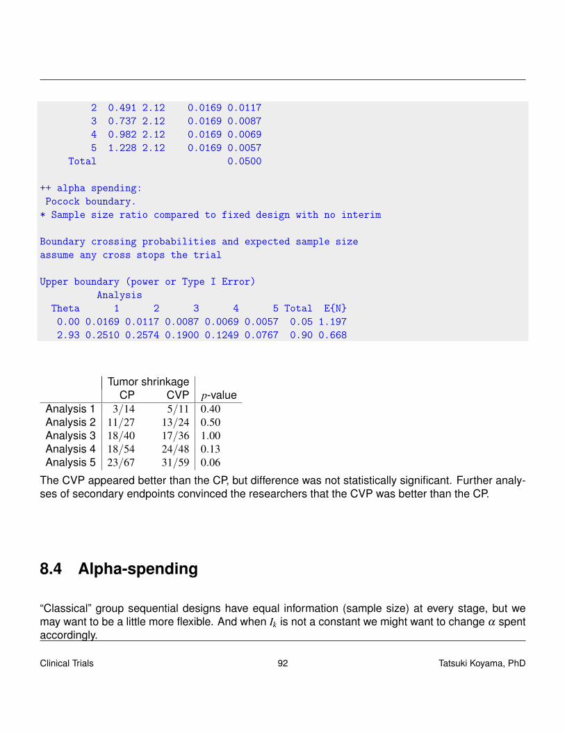
2 0.491 2.12 0.0169 0.01173 0.737 2.12 0.0169 0.00874 0.982 2.12 0.0169 0.00695 1.228 2.12 0.0169 0.0057

Total 0.0500

++ alpha spending:Pocock boundary.




Theta 1 2 3 4 5 Total E{N}0.00 0.0169 0.0117 0.0087 0.0069 0.0057 0.05 1.1972.93 0.2510 0.2574 0.1900 0.1249 0.0767 0.90 0.668

Tumor shrinkageCP CVP p-value

Analysis 1 3/14 5/11 0.40Analysis 2 11/27 13/24 0.50Analysis 3 18/40 17/36 1.00Analysis 4 18/54 24/48 0.13Analysis 5 23/67 31/59 0.06

The CVP appeared better than the CP, but difference was not statistically significant. Further analy-ses of secondary endpoints convinced the researchers that the CVP was better than the CP.

8.4 Alpha-spending

“Classical” group sequential designs have equal information (sample size) at every stage, but wemay want to be a little more flexible. And when Ik is not a constant we might want to change α spentaccordingly.


Decompose the rejection region.

R = P{|Zk| ≥ ck for some k = 1, · · · ,K}= P{(|Z1| ≥ c1) or (|Z1|< c1 and |Z2| ≥ c2) or · · ·}= P{|Z1| ≥ c1}+P{|Z1|< c1 and |Z2| ≥ c2}+P{|Z1|< c1 and |Z2|< c2 and |Z3| ≥ c3}+ · · ·= α(I1)+(α(I2)−α(I1))+(α(I3)−α(I2)−α(I1))+ · · ·

The biggest advantage of alpha-spending approach is its flexibility; neither the number nor timing ofthe interim analyses need to be specified in advance. The monitoring plan can be changed duringthe trial and still type I error rate is preserved. The power depends relatively little on the number andtiming of the interim looks1.

Alpha-spending functionsO’Brien-Fleming α(t) = 2

[1−Φ

(zα/2/

√t)]

Pocock α(t) = α log(1+(e−1)t)Kim-DeMets (Power) α(t,θ) = αtθ (for θ > 0)Hwang-Shih-DeCani α(t,φ) = α

1−e−φ t

1−e−φ (for φ 6= 0)

1“Fundamentals of clinical trials (4th ed)” by Friedman LM, Furberg CD, DeMets DL


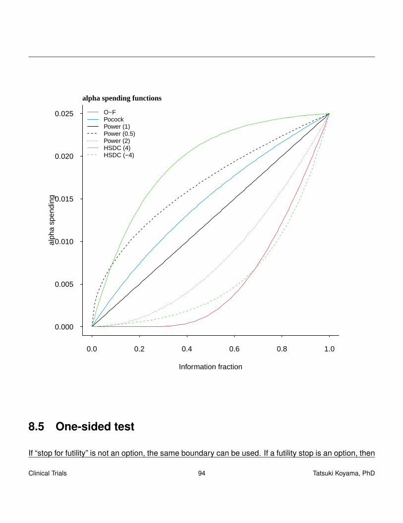
0.0 0.2 0.4 0.6 0.8 1.0

0.000

0.005

0.010

0.015

0.020

0.025

Information fraction

alph

a sp

endi

ng

O−FPocockPower (1)Power (0.5)Power (2)HSDC (4)HSDC (−4)

alpha spending functions

8.5 One-sided test

If “stop for futility” is not an option, the same boundary can be used. If a futility stop is an option, then


After group k = 1, · · · ,K−1if Zk ≥ bk stop and reject H0.if Zk ≤ ak stop for futility (accept H0).

After group Kif Zk ≥ bK stop and reject H0.if Zk < aK stop for futility.

Note that aK = bK ensures that the test terminates at analysis K.

8.6 Repeated confidence intervals

If we compute unadjusted confidence intervals Xso far± 1.96σ/√nso far at the end of each stage,

we get low coverage probabilities. Armitage, McPherson, Rowe (“Repeated significance tests onaccumulating data”. JRSS-A 1969) computed the actual coverage probabilities (Table 2).Number of looks Overall probability that

all intervals contain θ

1 0.952 0.923 0.894 0.875 0.86

10 0.8120 0.7550 0.68∞ 0

The idea of repeated confidence intervals (RCIs) is to use an adjusted value, ck(α,K), instead of1.96 so that the overall coverage probability is 1−α/2. The value of ck(α,K) is the critical value(border) for each stage and depends on α and K if Pocock boundary is used, and additionally k ifO’Brien-Fleming boundary is used.Example: Suppose we use a 6-stage group sequential design of O’Brien-Fleming type with a two-sided α = 5%. The critical values are:

gsDesign(k = 6, test.type = 2, alpha = 0.025, sfu = "OF")

Symmetric two-sided group sequential design with90 % power and 2.5 % Type I Error.Spending computations assume trial stopsif a bound is crossed.

SampleSize


Analysis Ratio* Z Nominal p Spend1 0.172 5.03 0.0000 0.00002 0.343 3.56 0.0002 0.00023 0.515 2.90 0.0018 0.00174 0.686 2.51 0.0060 0.00475 0.858 2.25 0.0123 0.00796 1.030 2.05 0.0200 0.0105

Total 0.0250

++ alpha spending:O'Brien-Fleming boundary.




Theta 1 2 3 4 5 6 Total E{N}0.00 0.0000 0.0002 0.0017 0.0047 0.0079 0.0105 0.025 1.0223.24 0.0001 0.0487 0.2350 0.2915 0.2088 0.1159 0.900 0.739


Theta 1 2 3 4 5 6 Total0.00 0 0.0002 0.0017 0.0047 0.0079 0.0105 0.0253.24 0 0.0000 0.0000 0.0000 0.0000 0.0000 0.000

The critical values are

[1] 5.03 3.56 2.90 2.51 2.25 2.05

First, let’s confirm that the critical values have the form ck =COB(K,α)√

IK/Ik. The final critical valueCOB(6,α) = 2.053, and assuming the looks are equi-distant (same group sample size), we have:

c1 = 2.053√

6/1 = 5.028 c2 = 2.053√

6/2 = 3.556

c3 = 2.053√

6/3 = 2.903 c4 = 2.053√

6/4 = 2.514

c5 = 2.053√

6/5 = 2.249 c6 = 2.053√

6/6 = 2.053


Then after stage 1, we would use 2.053 in place of the regular 1.96 when computing a 95% confidenceinterval. In general after stage k (k = 1, · · · ,6),

(xkt− xkc)± ck

√2σ2√

mk,

where m is per-group sample size for each stage.This method (RCI) is consistent with the corresponding hypothesis testing. Only when is H0 rejectedin stage k, the confidence interval for that stage will exclude the null value. Thus, we can use theidea of “inverting hypothesis test” to get the same confidence interval. (more later)

8.7 p-values

Recall how we construct a proper p-value for a Simon’s two-stage design in phase II methodology.We needed to define “more or as extreme as the observed data”. To be able to do this, we needto have an ordering of all the sample paths. In a simple single-stage design, the ordering is usuallybased on z-values (or absolute value of z-values if two-sided test), i.e., the bigger the observed z, thestronger the evidence against H0. Then a one-sided p-value is computed by

p = P0[Z ≥ z].

With a group sequential design, or more generally, with a multi-stage design with pre-specified group-wise sample sizes, the following orderings have been proposed. Notation: (k′,z′) � (k,z) to denote(k′,z′) is above (k,z).

• Stage-wise ordering.(k′,z′)� (k,z) if any of the following is true:

1. k′ = k and z′ ≥ z.

2. k′ < k and z′ ≥ bk′ (upper critical value).

3. k′ > k and z≤ ak (lower critical value).

• MLE ordering.(k′,z′) � (k,z) if z′/

√Ik′ > z/

√Ik. Originally proposed in connection with a test for a binomial

proportion The bigger value of the MLE gets a higher order. Sometimes called “sample meanordering” because this is equivalent to ordering based on the sample mean (one-sample) orthe difference of sample means (two-samples).

• Likelihood ratio ordering.(k′,z′)� (k,z) if z′ > z. (Stages do not matter.)


• Score test ordering.(k′,z′)� (k,z) if z

√Ik′ > z

√Ik.

Whichever ordering is used, we can compute a one-sided p-value is

P0[(T,ZT )� (k∗,z∗)]

For example, if we use a stage-wise ordering and test terminates in the K−1 stage with ZK−1 > bK−1(reject H0).

p =∫

∞

b1

g1(z;0)dz+ · · ·+∫

∞

z∗gK−1(z;0)dz.

In the above expression, gk(z;θ) is a density function of z in stage k. Conceptually, the densityfunction of z in k stage depends on all the data in the previous stages, 1 · · ·k−1, requiring multivariateintegration.Armitage, McPherson, Rowe (1969) derived a recursive formula so that the computation is muchsimplified, requiring only a succession of univariate integrations. For k = 2, · · · ,K,

gk(z;θ) =∫

Ck1

gk−1(µ;θ)

√Ik√∆K

φ

(z√

Ik−µ√

Ik−1−∆kθ√∆k

)dµ,

where Ck1 is the continuation region of the stage k1, and ∆k is the increment information, Ik− Ik−1.If stage-wise ordering is used, it automatically ensures that item the p-value is less than the signifi-cance level α if and only if H0 is rejected.Once we define the ordering to use with the group sequential test then we can compute a p-value fortesting H0 : θ = 0 by “inverting hypothesis test”. A (1−α/2) confidence interval is a collection of θ ′0such that H ′0 : θ = θ ′0 would be accepted with the observed sample path. (More details with generaladaptive designs.)


Chapter 9

General Adaptive Designs

Adaptive clinical trials

• are prospectively planned.

– All possible adaptations are defined in protocol.

• require much more forethought than a single stage design.

• require same level of evidence as usual.

• are accepted by regulators (e.g., FDA)

– FDA guidance availableGuidance for Industry: Adaptive Design Clinical Trials for Drugs and Biologics

• are nicer with the Bayesian method.

9.1 Introduction

Much of discussion in the literature for flexible designs in phase III clinical trial methodologies revolvesaround 2 stage designs. Practically speaking, implementing flexible Frequentist clinical trials beyondtwo stages is difficult, and perhaps these multi-stage flexible designs add only little to the designswith just two stages. Moreover, phase III clinical trials are for confirmatory purposes, and adaptivelychanging the design more than once in the middle of a confirmatory trial is not seen favorable by theregulatory figure.So we will only consider two-stage adaptive designs. Two-stage group sequential designs are exam-ples of such designs.


9.2 Background

We will look at unblinded two stage designs in which all the information from stage 1 is available.Design of the second stage (sample size and critical value) may be specified as functions of stage1 data. If both sample size and critical value are constants in stage 1 data, then it reduces to atwo-stage group sequential design.Adaptive designs can be categorized into the following two types:

• prespecified designsDesign of the second stage (e.g., sample size and critical value) is specified before the firststage. There is nothing to decide at the end of stage 1. The design of the second stage isdefined flexibility as functions of stage 1 data. Group sequential designs fall into this category.

• unspecified designsDesign of the second stage is not specified in advance and determined after stage 1 data areobserved. These designs are generally not accepted by the regulatory body.

Characteristics of these types of designs:

prespecified designs

• Type I error can be controlled.

• Type II error can be controlled; the power can be specified.

• Design characteristics (e.g., expected and maximum sample sizes) can be computed prior tothe initiation of the study.

unspecified designs

• Type I error can be controlled.

• These designs give much flexibility to handle unexpected situations (e.g., variance much biggerthan anticipated).

• Probably not accepted.

What they say about adaptive designs...

PhRMA (2006) “A clinical study design that uses accumulating data to decide how to modify aspectsof the study as it continues, without undermining the validity and integrity of the trial.”“... changes are made by design, and not on an ad hoc basis; therefore, adaptation is a designfeature aimed to enhance the trial, not a remedy for inadequate planning.”


EMA (2006) “A study design is called ‘adaptive’ if statistical methodology allows the modificationof a design element (e.g. sample-size, randomisation ratio, number of treatment arms) at aninterim analysis with full control of type I error rate.”“adaptive designs should not be seen as a means to alleviate the burden of rigorous planningof clinical trials.”

FDA (2010) “... adaptive design clinical study is defined as a study that includes a prospectivelyplanned opportunity for modification of one or more aspects of the study design and hypothesesbased on analysis of data (usually interim data) from subjects in the study.”

9.3 Conditional power

• Power is the probability of rejecting H0.

• Type I error rate is the power computed under H0.

• Conditional power is the probability of rejecting H0 at the end of the second stage conditionedon the first stage data.

Example: Suppose in stage 1, we will reject H0 if Z1 > 2.3 otherwise continue to stage 2. At the endof stage 2, we will reject H0 if Z2 > 2.1, where Z1 is from the stage 1 data, and Z2 is from the combineddata from both stages. Then

• Stage 1 power is P[Reject H0 at the end of stage 1] = P[Z1 > 2.3].

• Stage 2 conditional power is P[Reject H0 at the end of stage 2 | Stage 1 data] = P[Z2 > 2.1|Z1 =z1].

– If there is no stage 2, conditional power does not exist, but...

– we can let conditional power = 1 if H0 is rejected in stage 1 and = 0 if the trial stops forfutility in stage 1.

• Conditional type I error rate is the probability of rejecting H0 in stage 2 under H0 conditioned onthe stage 1 data.

Suppose

Z2 =Z1 +Z2−1√

2


where Z2 are from the cumulative data, and Z2−1 are from the stage 2 data only. Under H0 Z2 ∼Normal(0,1). Conditioned on Z1 = z1, we have

Z2 =z1 +Z2−1√

2.

Therefore, Z2 > c is equivalent to

Z2−1 >√

2c− z1.

# Stage 1 type I error rate1 - pnorm(2.3)

[1] 0.0107

# Conditional type I error rate:condTypeI <- function(z1) {

# Reject H0 if Z_2 > 2.1.1 - pnorm(2.1 * sqrt(2) - z1)

}# Conditional type I error rate if Z_1 = 0.condTypeI(0)

[1] 0.00149

# Conditional type I error rate if Z_1 = 1.condTypeI(1)

[1] 0.0244

# Conditional type I error rate if Z_1 = 2.condTypeI(2)

[1] 0.166

When planning a two-stage adaptive design, we need to make sure that the (unconditional) type Ierror rate is α, which is usually 2.5% To compute the unconditional type I error rate, or more generally,the unconditional power, we need to integrate the unconditional type I error rate (power) with respectto the distribution of Z1.


P[Unconditional power] =∫

P[Conditional power | Z1 = z1] f (z1)dz1

Integrand <- function(z1) {condTypeI(z1) * dnorm(z1)

}

## Stage 2 (unconditional) type I error rate.integrate(Integrand, lower = -Inf, upper = 2.3)$value

[1] 0.0138

Sometimes, the term, “predictive power” is confused with the conditional power. The predictive poweris a Bayesian concept, which is a weighted average of the power computed for different values of θ

with the weight is defined by the distribution of θ .In the above example, we used a simple test statistic

Z2 =Z1 +Z2−1√

2

to combine the data from both stages; however, this is rarely used in practice (despite its simplicity)because it puts the same weight on the stage 1 and 2 z-values regardless of the sample sizes.

9.4 Two-stage design -without all the math-

We will consider a simple situation, where we aim to test H0 : δ = 0, where δ = µt − µc. Randomsamples are taken from the treatment and control populations

Xt ∼ Normal(µt ,σ2t ) Xc ∼ Normal(µc,σ

2c ).

Assume the true variances are equal and known: σ2t = σ2

c = σ2. Also assume the stage 1 samplesizes are equal in the control and treatment groups: n1t = n1c = n1. Then

X1t ∼ Normal(µt ,σ2/n1) X1c ∼ Normal(µc,σ

2/n1)

and

Z1 =

√n1(X1t− X1c)√

2σ.


The distribution of Z1 under the null is Norlam(0,1).In stage 1, we observe Z1 and use the following decision rule:

• If Z1 < k1, stop for futility.

• If Z1 > k2, stop and reject H0.

• If k1 < Z1 < k2 then continue to stage 2.

In stage 2, we take a sample of size n2 from each arm, and define

Z2−1 =

√n2(X2t− X2c)√

2σ.

Conditioned on Z1 = z1 ∈ (k1,k2),

Z2−1 ∼ Normal(√

n2δ/(√

2σ),1),

which is Normal(0,1) under H0. Note that n2 may be a function of the stage 1 data.Instead of combining the stage 1 and 2 data with (Z1+Z2−1)/

√2, we will use the following test statistic

so that each X is weighted equally.

Z2 =

√n1√

n1 +n2Z1 +

√n2√

n1 +n2Z2−1.

We can write down the conditional distribution of this test statistic given Z1 = z1 (omitted).The important ideas here are:

• n2 is not a constant, but it is a random variable. n2(z1).

• When conditioned on Z1 = z1, Z1 is no longer a random variable but a constant.

• There are many decent ways to combine the stage 1 and 2 data.

• The critical value to use at the end of stage 2 can be for Z2−1, and it may be a function of Z1.

In the second stage, a sample of size n2(z1) is taken, and the decision rule at the end of stage 2 is:

• If Z2−1 ≤ c(z1), stop and conclude futility.

• If Z2−1 > c(z1), stop and conclude efficacy.


9.5 Conditional power functions

Like with the group sequential designs, we need to have the conditional type I error rate that satisfies

α = α1 +∫ k2

k1

P0[Reject H0|Z1 = z1]g(z1)dz1.

P0[Reject H0|Z1 = z1] is the conditional power, and we can use any form of conditional power as longas the above criterion is satisfied. Here let CP(Z1, δ ) to denote the conditional power function, sothat

CP(Z1, δ = δ0) is the conditional type I error rate.CP(Z1, δ = δ1) is the conditional power at the original alternative.

CP(Z1, δ = δ ) is the conditional power at the stage 1 trend.

9.6 Example

Design a two-stage procedure to test H0 : µt −µc = 0 and H1 : µt −µc > 0. Assume σ is known to be4. We want one sided α to be 0.025 and power to be 0.90 at µt − µc = 1. For a single stage design,the sample size is

N = 42(2)(z0.025 + z0.10)2

Stage 1 designLet’s decide to look at the data when n1 = 135 observations are available from each group. (approxi-mately 40% of N) We also need to decide how much of α and β we want to “spend” in stage 1. Let’schoose α1 = 0.01 and β1 = 0.025.

α1 = P0[Reject H0 in stage 1]= P0[Z1 > k2] where Z1 ∼ Normal(0,1)

Then k2 = 2.326.

β1 = P1[Accept H0 in stage 1]= P0[Z1 < k1] where Z1 ∼ Normal(

√n1ξ1,1) = Normal(2.05,1)


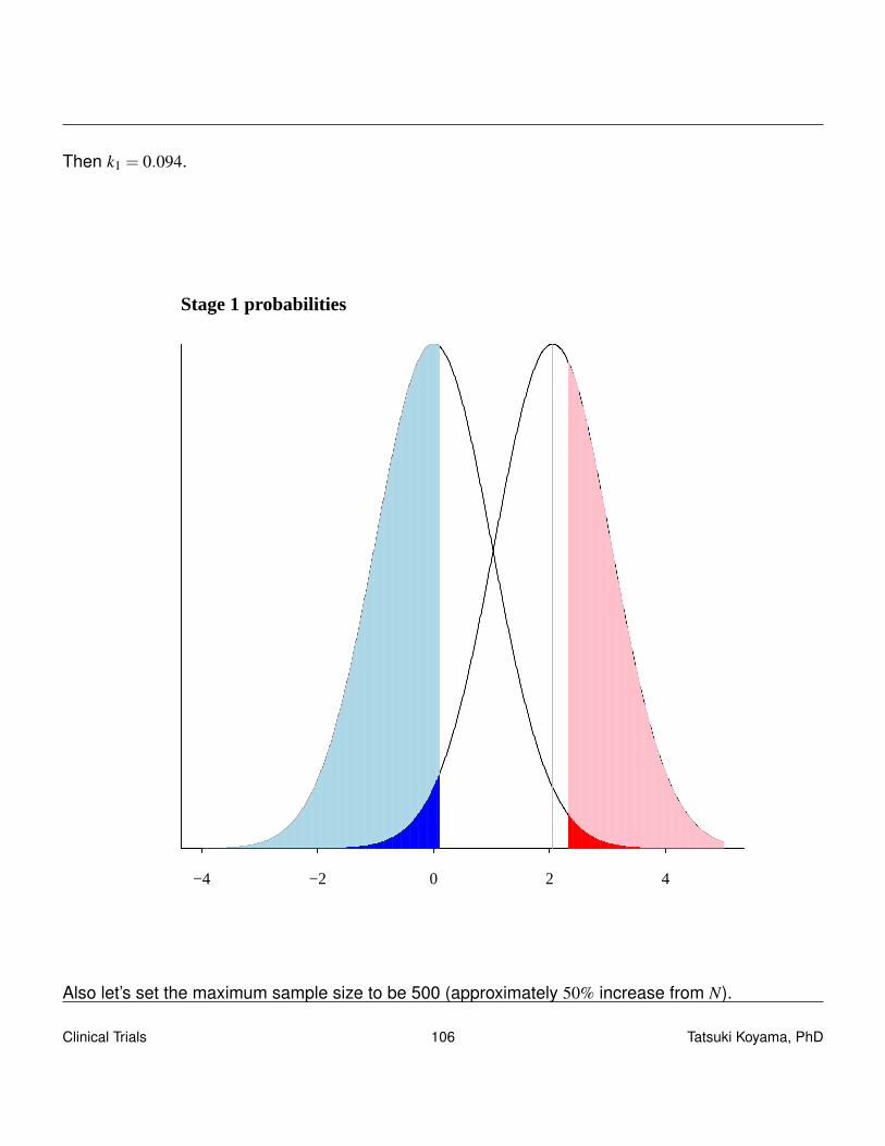
Then k1 = 0.094.

−4 −2 0 2 4

Stage 1 probabilities

Also let’s set the maximum sample size to be 500 (approximately 50% increase from N).


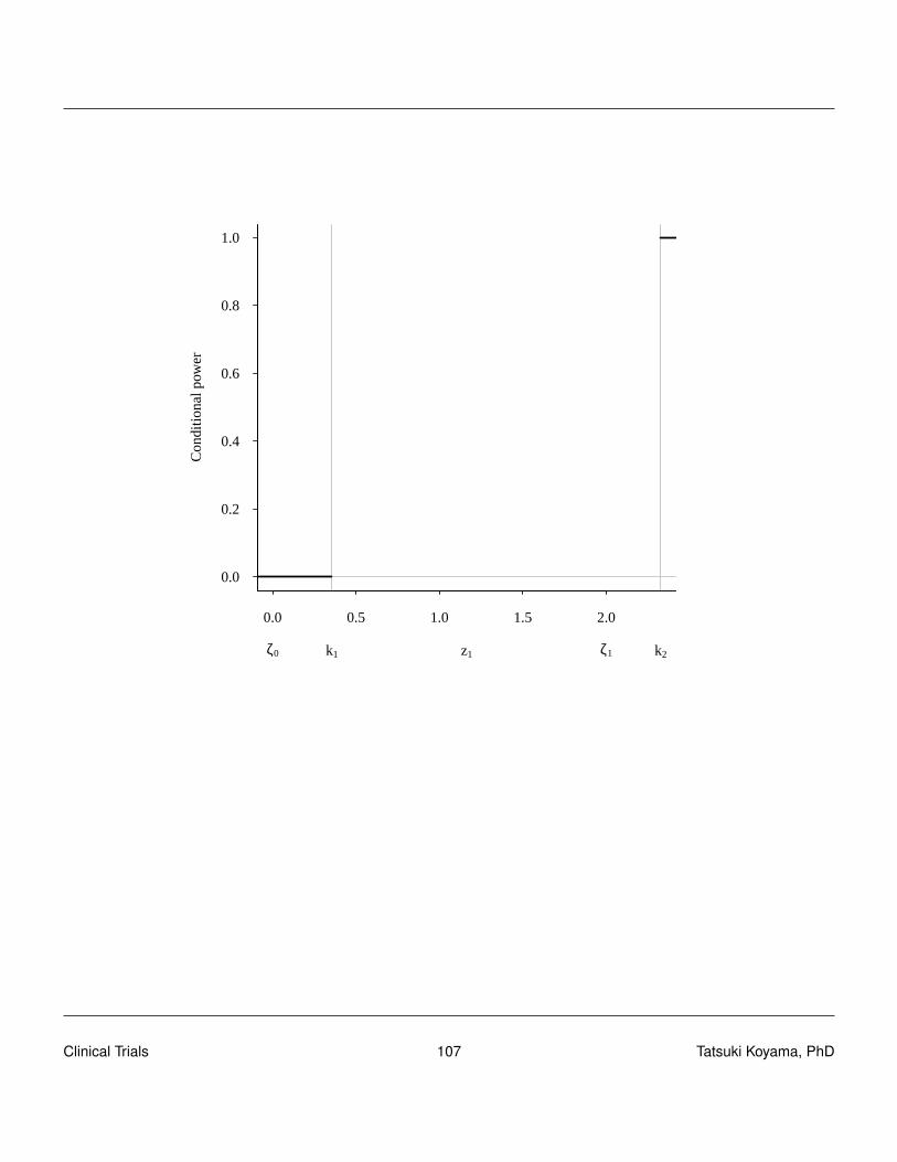
0.0 0.5 1.0 1.5 2.0

0.0

0.2

0.4

0.6

0.8

1.0

z1

Con

ditio

nal p

ower

ζ0 k1 ζ1 k2


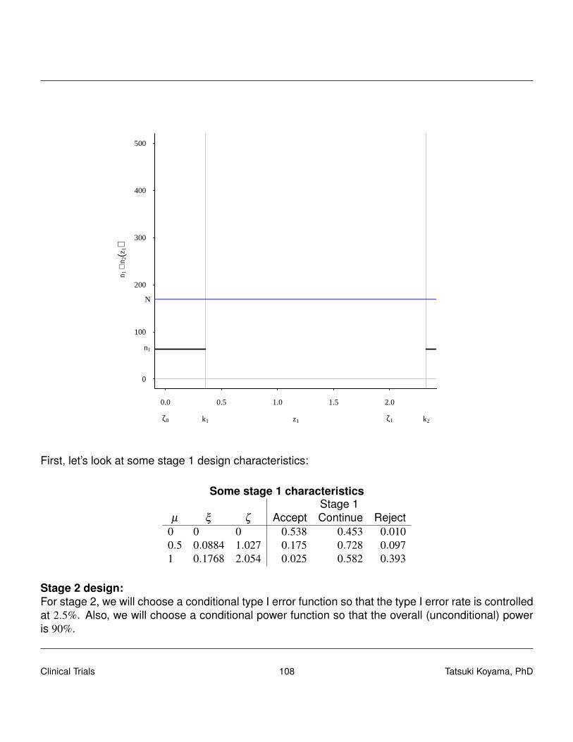
0.0 0.5 1.0 1.5 2.0

0

100

200

300

400

500

z1

n 1+

n 2(z

1)

ζ0 k1 ζ1 k2

n1

N

First, let’s look at some stage 1 design characteristics:

Some stage 1 characteristicsStage 1

µ ξ ζ Accept Continue Reject0 0 0 0.538 0.453 0.0100.5 0.0884 1.027 0.175 0.728 0.0971 0.1768 2.054 0.025 0.582 0.393

Stage 2 design:For stage 2, we will choose a conditional type I error function so that the type I error rate is controlledat 2.5%. Also, we will choose a conditional power function so that the overall (unconditional) poweris 90%.


– Some math –

We choose to use the following conditional type I error function:

CP(Z1,δ = δ0) = 0.002+5.255(z1− k1).

And the conditional power function:

CP(Z1,δ = δ1) = 0.75+1.004(z1− k1).

These two functions will satisfy the type I error rate condition (2.5%) and power condition (90%).

Now consider A-functions of the form A(z1,ξ0) = a0 +a1(z1− k1)2 and A(z1,ξ1) = b0 +b1(z1− k1). We

can use any A functions as long as they satisfy α and power conditions.

First we pick a0 (the value of A(z1,ξ0) at z1 = k1 to be 0.002 and solve for a1 so that

α2 = 0.015 =∫ k2

k1

A(z1,ξ0)g1(z1,ξ0)dz1.

Numerical integration finds a1 = 5.2547

A(z1,ξ0) = 0.002+5.2547(z1− k1)2.

Similarly for A(z1,ξ1), by specifying b0 = 0.75, we find b1 = 1.004 so that

A(z1,ξ1) = 0.75+1.004(z1− k1).

Using these two A functions, we can compute n2(z1), and it turns out max{n1 +n2(z1)}> 500, and weneed to modify the design a little. It is relatively simple to make small modifications to the design be-cause we understand how the design elements A(z1,ξ0), A(z1,ξ1), n2(z1), and c(z1), are interrelated.

First while fixing A(z1,ξ0), we “tap” n2(z1) so that max{n1+n2(z1)}= 500. This action changes A(z1,ξ1)slightly resulting a smaller power than 0.90. To make the power 0.90 again, we add a constant to thenew A(z1,ξ1) but capping the resulting n1+n2(z1) at 500. The final design is shown below graphically.


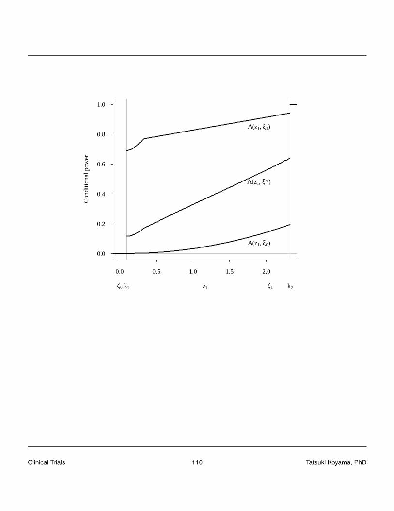
0.0 0.5 1.0 1.5 2.0

0.0

0.2

0.4

0.6

0.8

1.0

z1

Con

ditio

nal p

ower

ζ0 k1 ζ1 k2

A(z1, ξ0)

A(z1, ξ* )

A(z1, ξ1)


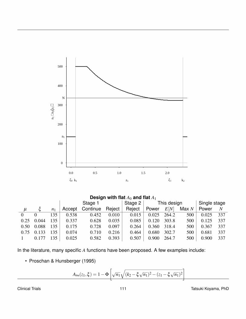
0.0 0.5 1.0 1.5 2.0

0

100

200

300

400

500

z1

n 1+

n 2(z

1)

ζ0 k1 ζ1 k2

n1

N

Design with flat A0 and flat A1Stage 1 Stage 2 This design Single stage

µ ξ n1 Accept Continue Reject Reject Power E[N] Max N Power N0 0 135 0.538 0.452 0.010 0.015 0.025 264.2 500 0.025 3370.25 0.044 135 0.337 0.628 0.035 0.085 0.120 303.8 500 0.125 3370.50 0.088 135 0.175 0.728 0.097 0.264 0.360 318.4 500 0.367 3370.75 0.133 135 0.074 0.710 0.216 0.464 0.680 302.7 500 0.681 3371 0.177 135 0.025 0.582 0.393 0.507 0.900 264.7 500 0.900 337

In the literature, many specific A functions have been proposed. A few examples include:

• Proschan & Hunsberger (1995)

APH(z1,ξ ) = 1−Φ

[√

n1

√(k2−ξ

√n1)2− (z1−ξ

√n1)2

]Clinical Trials 111 Tatsuki Koyama, PhD

• Chen, DeMets & Lan (2004)

ACDL(z1,ξ ) = 1−Φ

[√2zα − z1−ξ

√n1

]A(z1,z1) “Conditional power under the current trend”

9.7 Unspecified designs

The minimum requirement to control type I error rate is to pre-specify A(z1,ξ0) function that satisfiesα condition. Then after the first stage, when the actual z1 from the data are available, pick n2(z1) sothat conditional powers at any a value of ξ (other than ξ0) can be set.

If we allow even A(z1,ξ0) to be specified after the fist stage, type I error rate cannot be controlled.There exist many (in fact infinite number of) A(z1,ξ0) functions that give the desired value of α1 (0.01in our example). Depending on z1 the required sample size to guarantee a certain conditional powerdiffers. We cannot choose an A(z1,ξ0) function that gives the minimum sample size for the observedz1. Roughly speaking, when the conditional type I error rate at the observed z1 is large, the requiredsample size is small for the same conditional power. All three conditional type I error rates in thefollowing plot give α = 0.025.


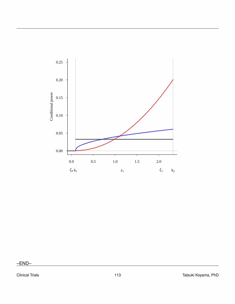
0.0 0.5 1.0 1.5 2.0

0.00

0.05

0.10

0.15

0.20

0.25

z1

Con

ditio

nal p

ower

ζ0 k1 ζ1 k2

–END–


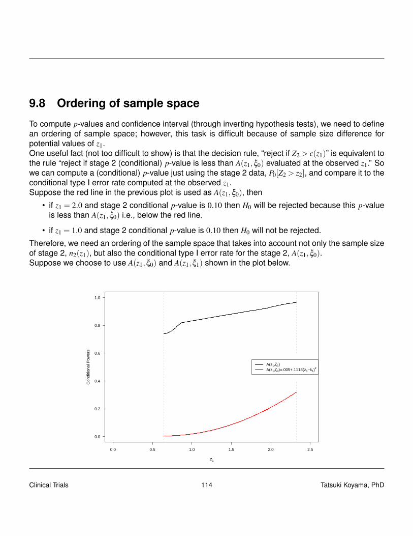
9.8 Ordering of sample space

To compute p-values and confidence interval (through inverting hypothesis tests), we need to definean ordering of sample space; however, this task is difficult because of sample size difference forpotential values of z1.One useful fact (not too difficult to show) is that the decision rule, “reject if Z2 > c(z1)” is equivalent tothe rule “reject if stage 2 (conditional) p-value is less than A(z1,ξ0) evaluated at the observed z1.” Sowe can compute a (conditional) p-value just using the stage 2 data, P0[Z2 > z2], and compare it to theconditional type I error rate computed at the observed z1.Suppose the red line in the previous plot is used as A(z1,ξ0), then

• if z1 = 2.0 and stage 2 conditional p-value is 0.10 then H0 will be rejected because this p-valueis less than A(z1,ξ0) i.e., below the red line.

• if z1 = 1.0 and stage 2 conditional p-value is 0.10 then H0 will not be rejected.

Therefore, we need an ordering of the sample space that takes into account not only the sample sizeof stage 2, n2(z1), but also the conditional type I error rate for the stage 2, A(z1,ξ0).Suppose we choose to use A(z1,ξ0) and A(z1,ξ1) shown in the plot below.

0.0 0.5 1.0 1.5 2.0 2.5

0.0

0.2

0.4

0.6

0.8

1.0

Z1

Con

ditio

nal P

ower

s

A(z1,ζ1)A(z1,ζ0)=.005+.1118(z1−k1)

2


And let’s consider the following 5 sample paths indicated by the conditional p values. Can we orderthe strength of evidence against H0 for these data?

0.0 0.5 1.0 1.5 2.0 2.5

0.0

0.2

0.4

0.6

0.8

1.0

Z1

Con

ditio

nal P

ower

s

A(z1,ζ0)=.005+.1118(z1−k1)2

• When z1 is the same, the second stage sample size is the same, so it should be simple to orderthe sampling paths. The smaller p value, the stronger evidence against H0.Blue � Red � Yellow.

• When the conditional p values are the same, then we can order them by the strength of evi-dence in the first stage.Blue � Black � Green.

• The black and red dots should indicate equal strength of evidence because they both result in“just” rejecting H0.

So in the above picture, the only unclear ordering is between Green and Yellow.The third rule gives a hint as to how to proceed; the data leading to the black and red dots indicatethat those data have just enough evidence to reject H0. The blue dot is for a sampling path that givesstronger evidence against H0; we could reject H ′0 that is more extreme.We can find a value of ξ ∗0 (equivalently, µ∗0 ) so that A(z1,ξ

∗0 ) goes through the blue dot, and say we

could have rejected H∗0 : µ = µ∗0 .


Technically speaking, we can find ξ ∗ by solving the following:

p = A(z1,ξ∗0 ) = 1−Φ

[c(z1)−

√n2(z1)ξ

∗0

]Note that p = P0[Z2 > z2], and once a value of z1 is observed, we can evaluate c(z1) and n2(z1), so theonly unknown quantity in the above expression is ξ ∗0 .From the above picture, we know the ordering is: Blue � Red = Black � Green � Yellow. And “someas or more extreme” than the observed is anything on and below the line, and we can compute thep-value by computing ∫

∞

k2

g1(z1,ξ0)dz1 +∫ k2

k1

A(z1,ξ∗0 )g1(z1,ξ0)dz1

0.0 0.5 1.0 1.5 2.0 2.5

0.0

0.2

0.4

0.6

0.8

1.0

Z1

Con

ditio

nal P

ower

s

A(z1,2.29)A(z1,.42)A(z1,.29)A(z1,0)A(z1,−.22)

This method (ordering) guarantees that the p-value and the corresponding hypothesis testing areconsistent (p-value < α iff H0 is rejected).And it can be shown that when n2(z1) and cu(z1) {critical value for the combined statistic} are con-stants, this ordering reduces to the stage-wise ordering.


9.9 Predictive power

With an unspecified design, some people are reluctant to use the conditional power to determine thedesign of the second stage. One issue is that where to compute the conditional power is not alwaysclear.The original alternative is usually a reasonable choice (A(z1,ξ1)). However, when the observed z1 ismuch different (smaller) from ξ1 we may not be interested in the conditional power at ξ1 but at somesmaller value that is still clinically meaningful. (Minimum clinically relevant alternative = ξ

†1 )

Another popular choice is ξ ≡ z1/√

n1 (“alternative under the current trend”).Or maybe we should compute the conditional power at somewhere in between ξ1 and ξ

†1 . Average?

Now we are talking like a Bayesian because we are talking about an average of ξs which are,for a frequentist, parameters. Maybe we have a prior distribution of ξ (or equivalently µ). And aposterior distribution of ξ after the first stage, π(ξ |z1), and we can compute a weighted average ofthe conditional power with respect to the posterior distribution. Something like∫

∞

−∞

A(z1,ξ )π(ξ |z1)dξ ,

and this is often called a predictive power given the stage one data.The conditional power is a frequentist concept, and it is computed at one value of ξ . The predictivepower is a Bayesian concept, and it is a weighted average of the conditional power with respect to aposterior distribution of ξ .


tatsuki koyama, phd

Documents