tata71 course programme, fall 2017

Hans LundmarkDepartment of MathematicsLinköping University

2017-12-07

ODEs and Dynamical Systems (TATA71)Course programme, fall 2017

General information

Ordinary Differential Equations and Dynamical Systems (TATA71) is an optional course for Mat2, Y4, M4,EMM4. It is given in the second half of the fall semester (period ht2). All information is publicly availableon the course webpage courses.mai.liu.se/GU/TATA71/. Lisam is not used in this course.

Literature

D. K. Arrowsmith & C. M. Place, Dynamical Systems: Differential Equations, Maps, and Chaotic BehaviourChapman and Hall/CRC (1992), ISBN 9780412390807.

Prerequisites

Basic courses in single-variable and multi-variable calculus/analysis, plus linear algebra.

Teaching

There will be 11 lectures and 11 lessons (problem-solving classes). See the lecture plan below.As always, it is a good idea to read (or at least skim) the relevant sections in the textbook before each

lecture, and also to try out a few of the problems before each lesson, since there will usually not be timeenough to do all of them in the classroom.

Examination

The examination consists of two parts:

• UPG1. Homework assignments, worth 2 hp (= 2 ECTS credits).

Some of the exercises for the lessons are assigned as homework problems (underlined in the programme),to be handed in continually during the course. These problems are only graded pass/fail, and if you fail aproblem, you simply hand in a corrected version later. It is allowed to discuss the problems with the teacherand with your fellow students, but please write the solution in your own words, don’t just copy someone else’ssolution! Handwritten solutions are fine, and you can write them in English or in Swedish.

Since this is a small course with few participants, there is probably no need to set any strict deadlines, butthe idea is that the homework problems are a way of giving you feedback, so the sooner you hand them in,the more useful they will be to you. And the intent is also that all problems should be completed before theChristmas break.

• TEN1. A written test (5 hours), worth 4 hp.

The test contains 6 problems, each of which is graded as pass (3 or 2 points) or fail (1 or 0 points). The totalgrade for the course is determined by the grade for the written test, which in turn is determined as follows: forgrade 3/4/5 (respectively), you need 3/4/5 passed problems and in addition at least 8/11/14 points in total.

1

http://courses.mai.liu.se/GU/TATA71/

What’s this course about?

As the name of the course suggests, we will study ODEs and dynamical systems.

• ODE is a standard abbreviation for ordinary differential equation, where the function that weseek depends on one variable. So an ODE is just a good old differential equation like those whichyou have already seen in your single-variable calculus course. We will also encounter systems ofODEs, involving several unknown functions at once, but each function will still only depend onone variable.

In contrast, a partial differential equation (PDE) is a differential equation where one seeks afunction depending on several variables, so that partial derivatives come into play.

• The idea of a dynamical system is rather broad, and it is hard to give a precise mathematicaldefinition which would cover every possible use of the phrase. But it refers to a “system” (whateverthat is) which changes in a deterministic way as time passes, and which is “memoryless” in thesense that (at any given instant) the future of the system is uniquely determined by the presentstate alone; the past is irrelevant.

We will usually assume when talking about dynamical systems that the laws governing the evolutiondon’t change with time. That is, if we start the system in a given state T units of time from now,we will get the same evolution as if we start it in that state right now (except that everything willbe delayed by T time units of course). If this needs to be emphasized, one uses the phrase auto-nomous dynamical system – a system which “runs on its own”, in contrast to non-autonomousdynamical systems where there may be some external time-dependent factors influencing theevolution of the system.

The state of the system is represented mathematically by an element of a set called the state space,typically Rn , or maybe some subset of Rn (like a cylinder, a sphere, or a torus). So one pictures theevolution of the system as the motion of a point in phase space.

• A discrete-time dynamical system is one where things happen at distinct time steps. We can useintegers to label the time steps, so that the system is in the state xn ∈ S at time n ∈ Z, where S is thestate space. Then the evolution of the system is simply specified by some function f : S → S:

xn+1 = f (xn), n ∈ Z.

(The system is autonomous since the function f is the same for all n.)

Discrete-time dynamical systems are a very important part of the general theory of dynamicalsystems, but will not be encountered much in this course.

• In a continuous-time dynamical system time passes smoothly, so we use real numbers to describetime, and talk about the system being in the state x(t ) at time t ∈ R. In this case, if the state spaceis Rn for simplicity, the evolution is determined by a system of first-order ODEs for the statex(t ) = (

x1(t ), . . . , xn(t )):

d x1/d t = f1(x1, . . . , xn),

d x2/d t = f2(x1, . . . , xn),

...

d xn/d t = fn(x1, . . . , xn),

or simply dx/d t = f(x) for short, with x ∈ Rn and f : Rn → Rn . (The system is autonomous since thefunction f doesn’t depend on t .)

In order for this to really define a dynamical system, we must impose suitable conditions on fwhich will guarantee existence and uniqueness of the solution to the ODEs for a given initialcondition, so that the future is uniquely determined by the present state.

2

Plan for lectures and lessons

Lecture 1. Basics of first-order ODEs 4

Lesson 1 6

Lecture 2. Phase portraits for two-dimensional systems 7

Lesson 2 8

Lecture 3. Two-dimensional linear systems 8

Lesson 3 10

Lecture 4. More about linear systems 10

Lesson 4 11

Lecture 5. Nonlinear systems, linearization at an equilibrium point 12

Lesson 5 13

Lecture 6. Stability theorems 13

Lesson 6 19

Lecture 7. Limit sets 19

Lesson 7 22

Lecture 8. Some applications 22

Lesson 8 23

Lecture 9. More about existence and uniqueness 23

Lesson 9 28

Lecture 10. Linear equations with non-constant coefficients 30

Lesson 10 36

Lecture 11. Outlook: Poincaré maps, attractors, chaotic systems 37

Lesson 11 37

3

[Back to lecture plan]

Lecture 1. Basics of first-order ODEs

(Arrowsmith & Place, sections 1.1, 1.2. And your old calculus textbook, if needed.)

This lecture introduces some basic ideas:

• Existence and uniqueness theorems for first-order ODEs d xd t = X (t , x).

Proposition 1.1.1 is usually called Peano’s existence theorem.

Proposition 1.1.2 is a slightly simplified version of the Picard–Lindelöf theorem. (The assumption“∂X /∂x exists and is continuous” is stronger than necessary; we’ll study this more thoroughly laterin the course.)

• How to find explicit solutions in simple cases.

(This is mostly a question of remembering the methods you have learned in previous courses. Seesummary below.)

• How to sketch the solution curves directly from the ODE.

• How to draw the phase portrait for a one-dimensional dynamical system.

A comment about notation

You might be used to ODEs looking something like this:

y ′′(x)+5y ′(x)+4y(x) = cos x (or simply y ′′+5y ′+4y = cos x),

where the independent variable is called x, and y = y(x) is the function that we seek. But since thisis a course about ODEs with a “dynamical systems perspective”, we will instead call the independentvariable t , for “time”, and use names like x(t) or y(t) for the sought functions. So the same ODE nowinstead looks as follows:

x ′′(t )+5x ′(t )+4x(t ) = cos t or x(t )+5x(t )+4x(t ) = cos t .

(It is common to use dots instead of primes to denote derivatives with respect to time.)

Two very fundamental examples

• Exponential growth/decay:x ′(t ) = r x(t ).

This is a linear equation, and we can solve it in several ways: integrating factor, characteristicpolynomial, separation of variables. Either way, the solution with initial condition x(0) = x0 is

x(t ) = x0 er t .

This will be encountered again and again in this course, and you will be expected to instantlyrecognize this equation and know its solution. Phase portrait (if r > 0): “←− 0 −→”.

• The logistic equation with growth rate r and carrying capacity K :

x ′(t ) = r x(t )

(1− x(t )

K

).

This nonlinear equation is often solved via separation of variables (followed by integration usingpartial fractions), but an easier way is to use the substitution x(t ) = 1/y(t ), since this is a Bernoulliequation. Solution, with x(0) = x0:

x(t ) = K x0

x0 + (K −x0)e−r t = K x0 er t

K + (er t −1)x0.

Here you don’t need to memorize the solution formula, but you should know roughly what thegraph of the solution x(t ) looks like for different values of x0. (In particular, x(t ) = 0 and x(t ) = Kare constant solutions.) Phase portrait (if r > 0 and K > 0): “←− 0 −→ K ←−”.

4


Summary of some exact solution methods

• Linear first order equations x ′+ax = b, where the coefficients a and b may be functions of thetime variable t :

x ′(t )+a(t ) x(t ) = b(t ).

How to solve: Find an antiderivative of a(t); call it A(t). Then multiply both sides of the ODE bythe integrating factor e A(t ), and use the product rule for derivatives (backwards). This gives(

e A(t ) x(t ))′ = e A(t ) b(t ),

which can now be integrated.

• Separable equations f (x) x ′ = g (t ).

What this means is that we seek x(t ) such that

f (x(t )) x ′(t ) = g (t ).

Integrating this with respect to t , using the chain rule (backwards), we immediately obtain thesolution in the implict form

F (x(t )) =G(t )+C ,

where F (x) is some antiderivative of f (x) and G(t) is some antiderivative of g (t). Ususally thisis remembered via the trick of writing x ′ = d x/d t and “separating the variables” by “multiplyingby d t”, and then attaching integral signs:

f (x)d x

d t= g (t ) ⇐⇒

∫f (x)d x =

∫g (t )d t .

It’s sometimes convenient to use definite integrals instead, particularly if we want to find a solutionsatisfying a given initial condition x(t0) = x0:∫ x(t )

x0

f (ξ)dξ=∫ t

t0

g (τ)dτ,

or in other wordsF (x(t ))−F (x0) =G(t )−G(t0).

As an important special case of separable equations we have one-dimensional dynamical systemsx ′ = a(x), which can always be solved by separation of variables:

x ′ = a(x) ⇐⇒ x(t ) = x∗ where a(x∗) = 0

or∫

d x

a(x)=

∫d t = t +C .

Warning! This method is full of pitfalls! Don’t forget the case a(x) = 0; there is a constant solutionx(t ) = x∗ for each zero x∗ of the function a(x). And one should also be very careful with handlinglogarithms and absolute values correctly when integrating and when simplifying the solution. Andin principle the constant of integration may be different in the different intervals into which thereal line is divided by the zeros of a(x). So if the ODE can be solved by some other method, it maybe wise to try that method first.

• Linear equations of arbitrary order:

x(n)(t )+an−1(t ) x(n−1)(t )+·· ·+a2(t ) x ′′(t )+a1(t ) x ′(t )+a0(t ) x(t ) = b(t ).

The general solution of such an equation has the structure

x(t ) = xhom(t )+xpart(t )

5


where xpart(t) is a particular solution and xhom(t) is the general solution of the correspondinghomogeneous equation which has 0 instead of b(t ) on the right-hand side.

Solving higher-order equations with time-dependent coefficients is usually a rather hopeless task,except that one may try to find solutions in the form of power series.

But it’s fairly easy in the special case of constant coefficients ak (t ) = ck :

x(n)(t )+ cn−1x(n−1)(t )+·· ·+c2x ′′(t )+ c1x ′(t )+ c0x(t ) = b(t ).

Then xhom(t ) can be found by looking at the roots of the characteristic polynomial

p(r ) = r n + cn−1 r n−1 +·· ·+c2r 2 + c1r + c0.

(If the roots are distinct and real, it’s easy. Repeated and/or complex roots are a bit harder.) To findxpart(t ) one usually makes a suitable Ansatz. See your calculus book for details about all this.

• If we start with x ′(t)+ a(t) x(t) = b(t), which we know that we can solve using an integratingfactor, and let x(t) = 1/y(t)k (for some k 6= 0), we get x ′(t) = −k y ′(t)/y(t)k+1, and consequentlyy(t ) satisfies the ODE

−ky ′(t )

y(t )k+1+a(t )

1

y(t )k= b(t ),

that is,

y ′(t )− a(t )

ky(t ) = b(t )

ky(t )k+1

The conclusion is that if we encounter an equation of this form, a so-called Bernoulli equation

y ′(t )+p(t ) y(t ) = q(t ) y(t )n ,

then we can reduce it to a linear equation by letting x(t ) = 1/y(t )n−1.

• Later in this course we will thoroughly study linear first order systems

x′(t ) = A(t )x(t )

where x(t ) = (x1(t ), . . . , xn(t )

)T is a column vector of functions and A(t ) is matrix of size n ×n. Butyou may already have seen in your linear algebra course how to solve such a system in the casewhere A is a constant matrix which happens to be diagonalizable: set x = My, where the columnsof M are linearly independent eigenvectors of A, and you get a decoupled system y′(t) = D y(t),where D is a diagonal matrix with the eigenvalues of A along the diagonal.

Lesson 1

The problems labelled A1, A2, etc., can be found in the section Additional problems just below. Theremaining problems (1.1, 1.2, etc.) are from the course textbook (Arrowsmith & Place), where they arelocated at the end of each chapter. Problems marked with an asterisk might be a bit more challenging.

• Solving ODEs using calculus techniques: 1.1, 1.2, 1.4, A1, A2.

• Sketching solution curves directly from the ODE: 1.11.

• Drawing phase portraits: 1.12, 1.13.

• Phase portraits for parameter-dependent ODEs: 1.14, 1.17*.

• Recovering the ODE from the family of solution curves: A3.

6


Additional problems for lesson 1

A1 Find the general solution for the following constant-coefficient second-order ODEs:

(a) x +6x +8x = t +2e−2t

[Answer: x(t ) = Ae−2t +Be−4t + (4t −3)/32+ t e−2t .]

(b) x +6x +9x = 0

[Answer: x(t ) = (At +B)e−3t .]

(c) x +6x +10x = 2e−3t cos t

[Answer: x(t ) = e−3t (A cos t +B sin t )+ te−3t sin t .]

A2 The Airy equation x(t) = t x(t) is a second-order ODE with non-constant coefficients. Find thesolution which satisfies x(0) = 1 and x(0) = 0, in the form of a power series x(t ) =∑∞

k=0 ak t k .

[Answer: x(t ) = 1+ t 3

2·3 + t 6

2·3·5·6 + t 9

2·3·5·6·8·9 + . . . ]

A3 A first-order ODE (usually) has a general solution constisting of a one-parameter family of curves.Here’s an opposite problem: Find an ODE x = X (t , x) such that the one-parameter family of curvest 2 +x2 = 2C t are solution curves.

(Hint: Differentiate t 2 +x(t )2 = 2C t with respect to t , and eliminate the parameter C from the twoequations.)

[Answer: x = (x2 − t 2)/2t x.]

Lecture 2. Phase portraits for two-dimensional systems

(Arrowsmith & Place, sections 1.3, 1.4, 1.5.)

Now we turn to two-dimensional dynamical systems

x1 = X1(x1, x2), x2 = X2(x1, x2),

where we assume that the functions X1 and X2 are nice enough to guarantee (local) existence anduniqueness of solutions. In vector notation: x = X(x). The function X should be thought of as a vectorfield in phase space: a vector is prescribed at each point x. The solution curves for the systems are curveswhose tangent vector x at each point agrees with the prescribed vector X(x); they are sometimes calledflow lines of the vector field.

• In very simple cases, we can solve the system explicitly. Sometimes we can obtain partial informa-tion by methods of calculus.

• But we can also get at least a rough idea of what the phase portrait looks like by direct inspectionof the signs of the functions X1(x1, x2) and X2(x1, x2).

• Syntax for drawing phase portraits in Mathematica or Wolfram Alpha (www.wolframalpha.com):

StreamPlot[X1(x, y), X2(x, y), x, xmin, xmax, y, ymin, ymax ]

For example:

StreamPlot[-1-x^2+y, 1+x-y^2, x, -3, 3, y, -3, 3]

(But don’t expect an automatic command like this to produce anything nearly as good as thehand-tuned graphics in the textbook.)

7

http://www.wolframalpha.com


• Arrowsmith & Place use the phrase fixed point for a point x∗ such that X(x∗) = 0, but I will usuallysay equilibrium point or just equilibrium, and you may come across many other synonyms too:rest point, critical point, steady state, etc.

The reason for the terminology is of course that x(t) = x∗ is a constant solution of the systemx = X(x) in this situation. That is, a system starting in the state x∗ remains in the state x∗ forever.

• The evolution operator or flow ϕ is the function which maps each point x in phase space to theplace where it will be t units of time later if moving as prescribed by the dynamical system. It isdenoted by ϕt (x) in the book, but it’s also common to write ϕ(t , x), since it is simply a function of tand x.

A fact which isn’t mentioned in the textbook is that the flowϕ is as “nice” as the vector field X. Moreprecisely, there’s a theorem which says that if the system is

x = X(x,λ),

whereλ= (λ1, . . . ,λN ) is some vector of parameters, and if X is of class C k (1 ≤ k ≤∞) as a functionof the variables (x,λ), then the flow ϕ is of class C k as a function of the variables (t ,x,λ).

Lesson 2

Underlined problems are homework problem to be handed in.

• Finding fixed points: 1.19ac.

In these problems, also find the nullclines (the curves where x1 = 0 or x2 = 0) and use this to drawthe regions of the phase plane where x1 and x2 are positive/negative).

• And another one for homework: 1.19d (including the follow-up question above about nullclinesand signs of x1 and x2.)

• Drawing families of parametrized curves and finding the corresponding ODEs: 1.20.

• Exact solution of a linear systems: 1.23 (draw the phase portrait both in the y1 y2-plane and in thex1x2-plane).

• An easy verification: 1.24.

• A nonlinear system which can be solved using polar coordinates: 1.25.

• Flows: 1.32, 1.36.

(Hint for 1.32, if you want to solve it from scratch: it’s a Bernoulli equation, let y = 1/x2. Or justuse separation of variables and partial fractions directly. Or else verify that the flow is correct, bycomputing d

d t ϕt (x0).)

Lecture 3. Two-dimensional linear systems


We will spend some time on understanding linear dynamical systems in two dimensions:

x1 = ax1 +bx2

x2 = cx1 +d x2⇐⇒

(x1

x2

)=

(a bc d

)︸︷︷︸

=A

(x1

x2

).

• Definition of a simple linear system: det(A) = ∣∣a bc d

∣∣ = ad − bc is nonzero. (Equivalently: theeigenvalues of A are nonzero.) This implies that the origin (x1, x2) = (0,0) is the only equilibriumpoint. In this lecture we’ll only consider simple systems.

8


• A linear change of variables x = My turns the system x = Ax into y = M−1 AMy.

• “Recipe” for choosing the columns m1 and m2 in the matrix M so that J = M−1 AM simplifies tothe Jordan normal form of A:

(a) Suppose A has two distict real eigenvaluesλ1 >λ2. Taking m1 and m2 to be the corresponding

eigenvectors gives J =(λ1 00 λ2

).

(b) Suppose A has a double real eigenvalue λ0. Then either A =(λ0 00 λ0

)is already in normal

form, or else there is just a one-dimensional eigenspace; in this case let m1 be an eigenvectorand take any vector not parallel to m1 as our preliminary m2. This will give a preliminary

J =(λ0 C0 λ0

)with some nonzero constant C . Adjust m2 by dividing it by this constant C ; this

will give the Jordan form J =(λ0 10 λ0

).

(c) Suppose A has a complex-conjugated pair of eigenvalues λ1,2 =α± iβ with β> 0.

This case is done in a very complicated way in the book (p. 39)! A much simpler way isto let a+ i b (with a and b real) be a complex eigenvector corresponding to the eigenvalue

λ1 = α+ iβ. Then m1 = b and m2 = a work, and directly give the Jordan form J =(α −ββ α

).

(These vectors must be linearly independent, otherwise they would both be real eigenvectorsof the real matrix A, with a non-real eigenvalue λ1, impossible.)

• How to solve the system y = Jy with a matrix in Jordan form, and how to draw its phase portrait.

In case (a) the phase portrait is a node or a saddle depending on the signs of the eigenvalues, incase (b) it is a star node or an improper node, and in case (c) it is a centre or a spiral (also calledfocus).

The phase portrait for x = My will be of the same type, only distorted by the linear transformation M .The columns m1 and m2 give the principal directions of the phase portrait.

• A solution method which isn’t mentioned in the book, but is sometimes convenient, is to rewritethe system as a single second-order ODE with constant coefficients, as follows. The derivative ofx1 = ax1 +bx2 is

x1 = ax1 +bx2.

The second term here, bx2, can be rewritten using the equations from the system:

bx2 = b(cx1 +d x2) = bcx1 +d(bx2) = bcx1 +d(x1 −ax1) = d x1 − (ad −bc)x1.

So we find that x1 = ax1 +(d x1 − (ad −bc)x1

), or in other words

x1 − (a +d)x1 + (ad −bc)x1 = 0.

This second-order ODE for x1(t ) can now be solved as in calculus, with the help of its characteristicpolynomial

p(λ) =λ2 − (a +d)λ+ (ad −bc),

which (perhaps not surprisingly) coincides with the characteristic polynomial of the system’smatrix A, as we can easily check:

p(λ) = det(A−λI ) =∣∣∣∣a −λ b

c d −λ∣∣∣∣= (a −λ)(d −λ)−bc =λ2 − (a +d)λ+ (ad −bc).

And once x1(t) is known, we also get x2(t) from x2 = (x1 −ax1)/b, assuming that b 6= 0. (If b = 0,the system is easy to solve right away: the first equation x1 = ax1 +0x2 gives x1(t ) = x1(0)eat ; plugthis into the second equation and solve it using an integrating factor or (x2)hom + (x2)part.)

9


Lesson 3

• A little reminder of how linear transformations work: 2.1.

• Transformation to canonical form: 2.3, 2.4.

• Solving canonical linear systems (and drawing the phase portrait): 2.8, 2.9.

Lecture 4. More about linear systems

(Arrowsmith & Place, sections 2.4, 2.5, 2.6, 2.7.)

• How to tell directly from the coefficients of the matrix A = (a bc d

)what the type of the phase portrait

for x = Ax is, without computing the eigenvalues: compute the trace and the determinant,

β= tr(A) = a +d , γ= det(A) = ad −bc,

and locate the point (β,γ) in the following diagram (cf. Figure 2.7 in the book):

β= tr(A)

γ= det(A)

non-simple system

centrestable star or improper node unstable star or improper node

γ= (β/2)2

saddle saddle saddle

stable node unstable node

stable spiral unstable spiral

For systems on the parabola γ= (β/2)2, the type is a star node if the matrix A equals a constanttimes the identity matrix, otherwise it’s an improper node.

Centres are always stable, and saddles are always unstable (according to the general definitions of“stable equilibrium” and “unstable equilibrium” that will be given later in the course).

• (In particular, the zeros of the polynomial p(z) = z2 −βz +γ both have negative real part if andonly if the coefficients satisfy β< 0 and γ> 0, i.e., if the point (β,γ) lies in the second quadrant inthe diagram above. This is a special case of the Routh–Hurwitz criterion, which determines for apolynomial of arbitrary degree whether all its zeros have negative real part.)

• The word “type” above refers to a kind of “algebraic type”, two linear systems being of the sametype if and only if they are related via a linear change of variables. Such changes preserve theeigenvalues, so (for example) an unstable node with λ1 = 5 and λ2 = 3 cannot be transformed intoan unstable node with λ1 = 43 and λ2 = 17.

We might want to introduce some looser type of equivalence instead, which will allow (for example)any two unstable nodes to be considered equivalent.

• Classification of qualitatively equivalent types of phase portraits for two-dimensional simplelinear systems. Under this equivalence relation (Definition 2.4.1) there are only four differenttypes:

10


(a) Stable node, star node, improper node or spiral. (“Stable but not centre.”)

(b) Centre.

(c) Saddle.

(d) Unstable node, star node, improper node or spiral. (“Unstable but not saddle.”)

(One subtle detail regarding Definition 2.4.1: They say that two systems are qualitatively equivalent if there isa continuous bijection f which maps the phase portrait of one system onto the phase portrait of the otherand preserves the orientation of the trajectories. But how do we know that this relation is symmetric? (Ifsystem A is equivalent to system B , then we want system B to be equivalent to system A as well.) For this tohold, the inverse f −1 must also be a continuous bijection. This isn’t necessarily true for continuous bijectionsin general; consider for example the function from the interval (−π,π] in R to the unit circle in R2 givenby f (t) = (cos t , sin t). But there is a famous and rather difficult theorem by Brouwer which says that for acontinuous bijection between two open sets in Rn the inverse is automatically continuous, so the definitionis actually correct as it stands.)

• Qualitative equivalence is also called topological equivalence.

(A stronger condition is C k -equivalence, where one requires the map f and its inverse f −1 to beof class C k instead of just continuous.)

• As an aside, we may also mention the slightly different notion of conjugacy, where one also requiresthe time parametrization of the trajectories to be respected. More precisely, two systems with flowsϕ and ψ are said to be topologically conjugate if there’s a continuous map f with continuousinverse f −1 such that

f ϕt =ψt f

for all t . That is, following the flow ϕ of one system for t units of time and then mapping over tothe other phase portrait is always the same as first mapping to the other phase portrait and thenfollowing that flow ψ for t units of time.

(And the systems are C k -conjugate if f and f −1 are of class C k .)

For example, a system whose phase portrait consists of concentric circles all traversed with thesame period T is topologically equivalent to a system whose phase portrait consists of concentriccircles traversed with different periods, but the systems are not topologically conjugate.

• The exponential function for square matrices P :

eP = exp(P ) = I +P + 1

2!P 2 + 1

3!P 3 + . . .

• The solution to x = A x isx(t ) = e At x(0).

(Here it’s important that A is a constant matrix, not time-dependent.)

• Affine systems x = A x+h(t ), also called non-homogeneous linear systems.

It’s easy if h is time-independent and Ax0 = h for some x0: just set y(t ) = x(t )+x0 to get y = Ay. Buteven if this doesn’t hold, an affine system can be solved using e−At as an integrating factor.

• Linear systems and Jordan form in n dimensions.

Lesson 4

• Using the trace–determinant criterion: 2.13.

• Phase portrait via change of variables: 2.14.

• Computing matrix exponentials: 2.22, 2.23ab, 2.23cd.

11


• Affine systems: 2.29abcd, 2.30.

• A three-dimensional linear system: 2.33.

• Solution corresponding to a 4×4 Jordan block: 2.35a.

Lecture 5. Nonlinear systems, linearization at an equilibrium point


Now back to nonlinear systems x = X(x), in the plane R2 for simplicity, but the results are valid in Rn too.We assume that the vector field X(x) is of class C 1, so that we have existence and uniqueness of solutions;this assumption is also needed for the linearization theorem below to be valid.

• Suppose that x∗ = (a1, a2) is an equilibrium point: X1(a1, a2) = X2(a1, a2) = 0. Since the functionsX1 and X2 are assumed to be of class C 1, they are also differentiable, which by definition meansthat

X1(a1 +h1, a2 +h2) = X1(a1, a2)︸︷︷︸=0

+ X1

∂x1(a1, a2)h1 + X1

∂x2(a1, a2)h2 + remainder,

X2(a1 +h1, a2 +h2) = X2(a1, a2)︸︷︷︸=0

+ X2

∂x1(a1, a2)h1 + X2

∂x2(a1, a2)h2 + remainder,

where the remainders tend to zero faster* than√

h21 +h2

2 as (h1,h2) → (0,0).

• If we discard the remainders, we get a linear system for h(t ) = x(t )−x∗:

h1 = X1

∂x1(a1, a2)h1 + X1

∂x2(a1, a2)h2,

h2 = X2

∂x1(a1, a2)h1 + X2

∂x2(a1, a2)h2,

or in matrix notation,

h = ∂X

∂x(x∗)︸︷︷︸

=A

h.

This system is called the linearization of the original system at the equilibrium point x∗. Itsmatrix A is the Jacobian matrix of X(x), evaluated at the equilibrium point x∗ (so it’s really just aconstant matrix).

• Our hope is that the linear system h = Ah (which we know how to analyze completely) will tell ussomething about the behaviour of the original nonlinear system x = X(x) near the point x∗.

And this is indeed the case, provided that x∗ is a hyperbolic† equilibrium point, meaning that theJacobian matrix A = ∂X

∂x (x∗) has no eigenvalues on the imaginary axis in the complex plane.

Under that condition, Theorem 3.3.1 (the linearization theorem) says that the nonlinear systemx = X(x) is indeed topologically equivalent‡ to its linearization h = Ah in a neighbourhood of x∗.

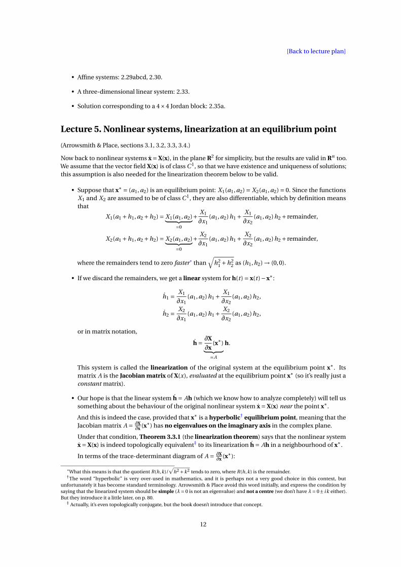
In terms of the trace-determinant diagram of A = ∂X∂x (x∗):

*What this means is that the quotient R(h,k)/√

h2 +k2 tends to zero, where R(h,k) is the remainder.†The word “hyperbolic” is very over-used in mathematics, and it is perhaps not a very good choice in this context, but

unfortunately it has become standard terminology. Arrowsmith & Place avoid this word initially, and express the condition bysaying that the linearized system should be simple (λ= 0 is not an eigenvalue) and not a centre (we don’t have λ= 0± i k either).But they introduce it a little later, on p. 80.

‡ Actually, it’s even topologically conjugate, but the book doesn’t introduce that concept.

12


β= tr(A)

γ= det(A)

no conclusion!

no conclusion!

saddle saddle saddle

stable unstable (and not saddle)

The linearization theorem is also called the Hartman–Grobman theorem, proved independentlyby Philip Hartman in the U.S.A. and D. M. Grobman in the Soviet Union around 1960. The proof israther difficult, and way beyond the scope of this course.§

(However, a simpler theorem, not dealing with topological equivalence but only with determiningstability based on linearization, can be proved using Liapunov’s theorems that we will learn aboutin the next lecture.)

Lesson 5

• Linearization: 3.5 (3.5eg), 3.6, 3.7 (3.7b).

• An isolated, but non-simple, fixed point: 3.8.

• Non-isolated fixed points: 3.11.

(To avoid confusion: here “a line of fixed points” rather means a curve.)

• An example regarding smoothness in the Hartman–Grobman theorem: A4*.


A4 Solve the system x = −x, y = −2y + x2 exactly and draw the phase portrait. Eliminate t to getexpressions y = y(x) for the solution curves; what degree of smoothness do they have at theorigin? Compare to the solution of the linearized system x =−x, y =−2y . Are the phase portraitsC 2-equivalent?

Lecture 6. Stability theorems


§For two-dimensional systems, a stronger result holds (also proved by Hartman): if the vector field X(x) is of class C 2, then thenonlinear system is actually C 1-conjugate (not just topologically conjugate) to its linearization, and moreover the derivative of theconjugating map at the origin is the identity. This means, for example, that if the linearization is a saddle, the eigenvectors will tellus the correct incoming and outgoing directions of the trajectories of the nonlinear system.

It is not true in three or more dimensions that we can always get C 1-conjugacy. However, it is true (as was proved as recently as2003) that the continuous conjugation map is differentiable at the origin, with the derivative there equal to the identity. (The proofassumes that X(x) is of class C∞, but the claim is conjectured to be true already for class C 2.)

It’s also not true (even in two dimensions) that one can get C k -conjugacy with k ≥ 2 by assuming the vector field to be nicer; seeproblem A4 for a counterexample with a vector field of class C∞ where one doesn’t get more than C 1-conjugacy.

13


• Definitions 3.5.1–4: The definition of a stable equilibrium (sometimes called Liapunov stable).Some stable equilibria are asymptotically stable. And those which are stable but not asymptot-ically stable are called neutrally stable. So there are exactly those two types of stable equilibria.Unstable equilibrium simply means an equilibrium which is not stable.

• The Russian name Liapunov can be translitered into the Latin alphabet in many ways. In English,Lyapunov is also very common, and one may also come across Ljapunow, Liapounoff, and so on.Anyway, it’s pronounced with the stress is on the last syllable: “-OFF”.

• Theorem 3.5.1 is Liapunov’s stability theorem (1892).

This theorem is useful for showing stability in situations where linearization is inconclusive.Even more importantly, it also provides a domain of stability; that is, a neighbourhood N of anasymptotically stable equilibrium x∗, such that any solution which starts in N stays in N andconverges to x∗ as t →∞. (From linearization we can only say that if all eigenvalues have negativereal part, then there is some domain of stability, but we don’t get any clue about the size of thatdomain.)

However, Arrowsmith & Place don’t state exactly how to find a domain of stability, and their proofof the theorem is also rather unclear. I will try to give more precise statements here.

First let us fix some terminology.

Definition. Let I be a proper* interval in R, and let f be a real-valued function whose domain ofdefinition contains I . The function f is said to be strictly decreasing on I if

f (t1) > f (t2)

whenever t1 ∈ I , t2 ∈ I and t1 < t2. It is weakly decreasing on I if

f (t1) ≥ f (t2)

whenever t1 ∈ I , t2 ∈ I and t1 < t2.

Remark. Any function which is strictly decreasing is weakly decreasing as well.

Remark. In English, it is more common to say decreasing and non-increasing instead of strictlydecreasing and weakly decreasing, but I have chosen the latter option here to reduce the riskof confusion with the usual terminology in Swedish, which is strängt/strikt avtagande and av-tagande, respectively. (And similarly in German and French.)

From now on we consider some fixed dynamical system x = X(x) in Rn , where the vector field X isdefined in some open set S ⊆ Rn , and we assume that V : Ω→ R is a differentiable function definedon some open setΩ⊆ S. (And of course we assume thatΩ and S are not the empty set, since thatwouldn’t be very interesting.)

Definition. The function V : Ω→ R is the dot product of the gradient ∇V and the vector field X:

V (x) =∇V (x) ·X(x), x ∈Ω.

Theorem. Suppose V (x) < 0 for all x ∈Ω. Then, for any solution x(t ) of the system which stays inthe setΩ during some nonempty open time interval I , the function

f (t ) =V (x(t )), t ∈ I

is strictly decreasing on I . If instead V (x) ≤ 0 for all x ∈Ω, then f is weakly decreasing on I . And ifV (x) = 0 for all x ∈Ω, then f is constant on I .

* A proper interval is an interval (in R) which contains infinitely many points, as opposed to the degenerate intervals [a, a] = aand ;= .

14


Proof. The chain rule gives

f ′(t ) =∇V (x(t )) · x(t )

=∇V (x(t )) ·X(x(t )) = V (x(t )), t ∈ I .

So if we know that V < 0 everywhere inΩ, and that x(t ) stays inΩ, then we have f ′(t ) < 0 for t ∈ I ,which implies that f is strictly decreasing on I (by a very basic calculus theorem). Similarly if V ≤ 0or V = 0.

Theorem (Liapunov’s stability theorem, weak version). Let x∗ be an equilibrium point of thedynamical system x = X(x), x ∈ S ⊆ Rn . Suppose that there is a weak Liapunov function, i.e., adifferentiable function V : Ω→ R defined on some open setΩ⊆ S containing x∗ and satisfying theconditions

1. V (x∗) = 0 and V (x) > 0 for all x ∈Ω\ x∗,

2. V (x) ≤ 0 for all x ∈Ω.

Then the equilibrium x∗ is stable.

Remark. As the theorem is formulated, the function V : Ω→ R has exactly the setΩ as its domainof definition. Usually we have some nice function V (typically a polynomial) which is definedeverywhere to begin with. What we actually do then is that we compute V , use that to locate someopen setΩwhere the assumptions of the theorem are fulfilled, and then apply the theorem with Vequal to the restriction of the original V to the setΩ.

Outline of proof. If U is any neighbourhood of x∗, let B ⊂U ∩Ω be a closed ball centered at x∗ andset

U ′ = x ∈ B : V (x) <α

,

where α > 0 is the minimum of V on the boundary sphere ∂B . Then U ′ ⊂ B ⊂ U , and U ′ is aneighbourhood of x∗ such that trajectories starting in U ′ can’t leave U (in fact, they can’t evenleave U ′).

Detailed proof. Let U be an arbitrary neighbourhood of x∗. To prove stability, we need to findanother neighbourhood U ′ such that solutions starting in U ′ will never leave U . To find U ′ webegin by taking a closed ball

B = B(x∗,ε) = x ∈ Rn :

∣∣x−x∗∣∣≤ ε

centered at x∗, with radius ε> 0 small enough for B to be contained inside both U andΩ. (This ispossible since U andΩ are neighbourhoods of x∗.) The boundary

∂B = x ∈ Rn :

∣∣x−x∗∣∣= ε

is a sphere of radius ε centered at x∗. This sphere is a compact set (closed and bounded), and Vis continuous by assumption, so according to the extreme value theorem V has a smallest valueon ∂B :

α= minx∈∂B

V (x).

In other words, there is a point x0 ∈ ∂B such that

α=V (x0) ≤V (x) for all x ∈ ∂B .

Since V is positive definite onΩ and we have chosen B small enough to be a subset ofΩ, we haveV (x) > 0 for all x ∈ ∂B , in particular

α=V (x0) > 0.

15


Now setU ′ =

x ∈ B : V (x) <α.

Then U ′ contains x∗, since V (x∗) = 0 <α. And U ′ is an open set, since V is continuous.† In otherwords, U ′ is an open neighbourhood of x∗. Moreover, a trajectory x(t ) starting in U ′ (at t = 0, say)can’t leave U . Here’s why: to leave U , the trajectory would have to leave B to begin with (sinceU ′ ⊂ B ⊂U ), and it’s a continuous curve so it would have to intersect the boundary sphere ∂B inorder to get out. But f (t) =V (x(t)) is a weakly decreasing function of t as long as x(t) stays in B(since B ⊂Ω, and V ≤ 0 inΩ by assumption). Since we start in U ′, we have f ′(0) <α, and hencef (t ) <α for t ≥ 0. So it’s impossible for the trajectory to reach ∂B , since that would mean f (t ) ≥αfor some t > 0. (In fact, the trajectory can’t even leave U ′ – as soon as it did, it would mean thatf (t ) ≥α.)

(One more technical detail: since the trajectory stays inside the compact set B , it must exist for allt ≥ 0; there can’t be any “blowup in finite time”. We haven’t proved that theorem in this course, sowe’ll just accept this fact on faith here.)

Theorem (Liapunov’s stability theorem, strong version). Let x∗ be an equilibrium point of thedynamical system x = X(x), x ∈ S ⊆ Rn . Suppose that there is a strong Liapunov function, i.e., adifferentiable function V : Ω→ R defined on some open setΩ⊆ S containing x∗ and satisfying theconditions

1. V (x∗) = 0 and V (x) > 0 for all x ∈Ω\ x∗,

2. V (x) < 0 for all x ∈Ω\ x∗.

Then the equilibrium x∗ is asymptotically stable. In fact, for any closed ball B = B(x∗,r ) containedinΩ, the set

N = x ∈ B : V (x) <α

, where α= minx∈∂B

V (x),

is a domain of stability: solutions starting in N stay in N , and converge to x∗ as t →∞.

Remark. IfΩ= Rn and if the additional condition

V (x) →∞ as |x|→∞holds, then for any given point x0 ∈ Rn it is true that

minx∈∂B

V (x) >V (x0)

if we take B large enough. This means that x0 ∈ N for that choice of B , causing the trajectorystarting at x0 to converge to x∗. So in this case x∗ is stable and every trajectory of the systemconverges to x∗, which is expressed by saying that x∗ is globally asymptotically stable.

Remark. If one studies the proof, it should be clear that the set B in the definition of N doesn’t reallyhave to be precisely a closed ball, just something which is topologically equivalent to a ball. Forexample, if our Liapunov function is V (x, y) = x6+y4, then for k > 0 the sublevel set B = x6+y4 ≤ kis sufficiently “ball-like” for the proof to work: no continuous curve can pass from the interior tothe exterior without crossing the closed level curve ∂B = x6 + y4 = k. The same arguments as inthe proof then show that trajectories can’t leave the set N = x ∈ B : V (x, y) < k = x6 + y4 < k, soprovided that B is contained in the regionΩ, N is a domain of stability for the equilibrium (0,0).

Outline of proof. Stability follows from the weak version of Liapunov’s theorem. Any trajectorystarting in N must stay in N , and along such a trajectory the function V decreases strictly towardssome limit L ≥ 0. But L > 0 would contradict the continuity of the flow ϕt , so L = 0, which in turnimplies that the trajectory converges to x∗ (the only point where V = 0).

† Take any x ∈ U ′, or in other words any x ∈ B with V (x) < α. Then actually x is in the interior of B , since V ≥ α on theboundary ∂B . Continuity of V at x means that there is an open ball B2 = B(x,δ) where V <α, and this ball must also be containedin the interior of B , for the same reason. So B2 ⊆U ′. Thus any x ∈U ′ has an open neighbourhood contained in U ′, and this isexactly what it means for U ′ to be open.

16


Detailed proof. Stability follows from the weak version of Liapunov’s theorem. As in the proofof that theorem, we see that N (as defined above) is an open neighbourhood of x∗, and that anytrajectory x(t ) starting in N stays in N and is defined for all t ≥ 0. For the constant solution x(t ) = x∗there is nothing to prove – of course it converges to x∗! So suppose x(t) is some other solutionstarting in N . Then, by the assumption V < 0, V (x(t)) is strictly decreasing function of t on theinterval t ≥ 0, and it’s bounded below (since V ≥ 0), so it has a limit L ≥ 0 as t →∞.

We want to show that L = 0, so assume L > 0 in order to get a contradiction. Take any sequence ofpositive numbers tn ∞; then xn = x(tn) is a sequence of points in the compact set B . Accordingto the Bolzano–Weierstrass theorem, a standard theorem about compact sets in Rn , this sequenceof points must have a convergent subsequence, i.e., there is a point y ∈ B and an integer sequencenk ∞ such that xnk → y as k →∞. Since V is continuous, V (y) = limk→∞V (xnk ) = L. We areassuming L > 0, which means that y 6= x∗ (since V is positive definite), and V will thus continue todecrease strictly along the trajectory starting at y. So the flow ϕ1, for example (or ϕt for any fixedt > 0), will map y to a point where V < L. But ϕ1 is a continuous function, so it will also map allsufficiently nearby points xnk to points where V < L:

V (ϕ1(xnk )) =V (x(1+ tnk )) < L, for all sufficiently large k.

But we know that V (x(t)) > L for all t ≥ 0, since V (x(t)) is decreasing towards the limit L. Thiscontradiction shows that the assumption L > 0 must have been incorrect. Hence L = 0.

Now we know that V (x(t)) L = 0 as t →∞. It remains to show that this implies x(t) → x∗, i.e.,that for any ε> 0 there is a time τ such that x(t) ∈ Bε for all t > τ, where Bε = B(x∗,ε) is the openball of radius ε centered at x∗. We may assume that 0 < ε< r , where r is the radius of the closedball B . Then

B \ Bε = B(x∗,r ) \ B(x∗,ε)

is a compact nonempty set, so the continuous function V has a smallest value β on this set (andβ> 0 since V is positive definite). What this means is that if x ∈ B and V (x) <β, then x ∈ Bε. But wehave x(t ) ∈ B for all t ≥ 0, and since V (x(t )) 0 as t →∞ there is a τ such that V (x(t )) <β for t > τ.Consequently x(t ) ∈ Bε for t > τ, as desired.

• The very useful Theorem 3.5.2 is an improvement of Liapunov’s theorem which is due to LaSalle(1960). It allows us to conclude asymptotic stability using only a weak Liapunov function, providedan additional condition is satisfied. The proof is not given in the book, but it is a consequence ofsomething called LaSalle’s invariance principle (see the next lecture).

Theorem (LaSalle’s stability theorem). Let x∗ be an equilibrium point of the dynamical systemx = X(x), x ∈ S ⊆ Rn . Suppose that there is a weak Liapunov function V : Ω→ R on some open setΩ⊆ S containing x∗, and in addition suppose that the set

x ∈Ω : V (x) = 0

contains no complete trajectories except x∗.

Then the equilibrium x∗ is asymptotically stable, and N (defined as in the strong version ofLiapunov’s theorem) is a domain of stability.

(And ifΩ= Rn and V (x) →∞ as |x|→∞, then x∗ is globally asymptotically stable.)

Proof. See the next lecture.

• Here is a somewhat subtle point concerning the above theorems and weak Liapunov functions. Ifwe have a function V which is everywhere defined and nice (continuously differentiable), thenthe set Ω1 of all x where V (x) ≤ 0 holds will be closed. But the theorems, as they are formulatedabove, require us to restrict V to an open setΩ. So we have to shrinkΩ1 “by hand” to get an opensetΩwhere V ≤ 0 holds. The purpose of this, as well as all the business with closed balls contained

17


insideΩ, is to avoid accidentally making plausible-sounding claims which are actually false. Weknow that V is weakly decreasing along trajectories, but only as long as they stay inΩ, so we needto take some precautions to prevent the trajectories from sneaking out ofΩ!

Example. If the system is x = y , y =−x − y(1−x2), and if V (x, y) = x2 + y2, then V =−2y2(1−x2)which is ≤ 0 on the setΩ1 which is the union of the closed strip −1 ≤ x ≤ 1 and the line y = 0. Soany trajectory will be moving closer to the origin (or at least not further away from it) as long as itis inside the strip, but trajectories for y > 3 (or so) will enter the strip from the left, leave it againon the right (a little further down), and then go off steeply upwards towards infinity instead ofconverging towards the equilibrium (0,0). So for example, a set like (x, y) ∈Ω1 : V (x, y) ≤ 100 isnot forward invariant despite V being weakly decreasing on trajectories in Ω1! But we can takeΩ to be the open strip −1 < x < 1, let B be any closed ball x2 + y2 ≤ k with 0 < k < 1 so that itfits inside Ω, and then the set N given by x2 + y2 < k will be a domain of attraction by LaSalle’stheorem, since there are no trajectories contained in the line y = 0 except the equilibrium solution(x(t ), y(t )) = (0,0). And since this is true for any 0 < k < 1, in fact the open unit disk x2 + y2 < 1 is adomain of attraction.‡

• Theorem 3.5.3 is Liapunov’s instability theorem.

• We have relied upon the rather deep Hartman–Grobman theorem to show that an equilibrium isasymptotically stable if the linearization there is asymptotically stable. This fact can be provedmore directly using Liapunov’s stability theorem. The simplest case is when the Jacobian ma-trix A = ∂X

∂x (x∗) has distinct real eigenvalues (assumed negative, in order for dh/d t = A h to beasymptotically stable):

0 >λ1 > ·· · >λn .

Make the usual linear change of coordinates x = My, where the columns of M form a basis ofeigenvectors of A. In terms of these coordinates, we have a system y = Y(y) with an equilibrium y∗where the Jacobian is diagonal:

J = ∂Y

∂y(y∗) = diag(λ1, . . . ,λn).

So k = y−y∗ satisfies

k = J k+ remainder,

where the remainder tends to zero faster than |k|. It’s not too difficult to check that V (k) =∑k2

i isa strict Liapunov function for this system in a neighbourhood of k = 0, which proves asymptoticstability. With repeated and/or non-real eigenvalues things are a bit more complicated, but if alleigenvalues have negative real part one can find a strong Liapunov function in the form of a sumof squares in those cases too.

Similarly, one can use Liapunov’s instability theorem to prove that if some eigenvalue has positivereal part, then the equilibrium is unstable.

• The flow box theorem. Global phase portraits.

• First integrals, also known as constants of motion, integrals of motion, conserved quantities,invariants, etc.

(Can sometimes be found by writing d y/d x = y/x = Y (x, y)/X (x, y) and solving the resulting ODEfor y = y(x).)

‡We can actually do yet a little better: the closed unit disk x2 + y2 ≤ 1 is forward invariant since the open unit disk is; this followsfrom the continuity of the flow, since if ϕt (for some t > 0) would map some point on the unit circle to a point outside the circle,then by continuity it would also have to map some nearby point inside the circle out of the circle, which we know it doesn’t. So theclosed unit disk is compact and forward invariant, and then we can try applying LaSalle’s invariance principle (see next lecture) toit. This turns out to be successful (exercise), so actually the closed unit disk is a domain of attraction.

18


• If H(p, q) is any C 1 function, then the Hamiltonian system(pq

)=

(∂H/∂q

−∂H/∂p

)=

(0 1−1 0

)∇H

automatically has H as a first integral. A fundamental fact in mechanics is that the Hamiltoniansystem generated by H(p, q) = 1

2 p2 +V (q) is equivalent to the Newton-type equation q =−V ′(q).(This works also in higher dimensions, with vectors p and q instead.)

Lesson 6

• Using strong Liapunov functions: 3.13abe, 3.14abe.

• Using weak Liapunov functions: 3.15, 3.17bc.

• Finding a domain of stability using a less obvious Liapunov function: 3.19b, 3.18*.

• Liapunov’s instability theorem: 3.22.

• Illustration of an explicit transformation which straightens out a nonlinear vector field: 3.24.

• First integrals (constants of motion): 3.28ab, 3.29*.

In 3.28b, you can do better than the answer in the book, and find a constant of motion which isactually defined for all x1 and x2!

In 3,29, you should do much better than the answer in the book, which is actually wrong. A correctconstant of motion is F (x1, x2) = x1(x2

1 − x2)/(x21 + x2)2. The level curves of this function are not

easy to plot by hand, but you can of course do it on the computer if you want to see what the phaseportrait looks like.

• An example§ illustrating why the requirement about stability in the definition of asymptoticstability is necessary: A5.


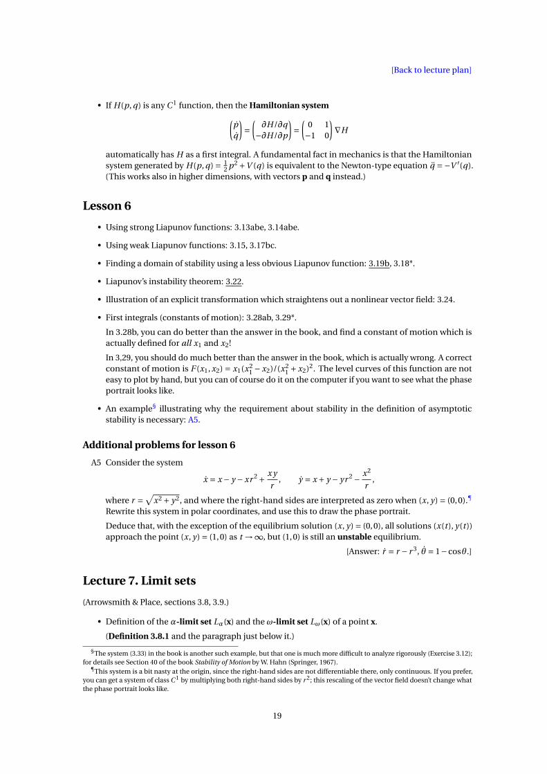
A5 Consider the system

x = x − y −xr 2 + x y

r, y = x + y − yr 2 − x2

r,

where r =√

x2 + y2, and where the right-hand sides are interpreted as zero when (x, y) = (0,0).¶

Rewrite this system in polar coordinates, and use this to draw the phase portrait.

Deduce that, with the exception of the equilibrium solution (x, y) = (0,0), all solutions (x(t ), y(t ))approach the point (x, y) = (1,0) as t →∞, but (1,0) is still an unstable equilibrium.

[Answer: r = r − r 3, θ = 1−cosθ.]

Lecture 7. Limit sets

(Arrowsmith & Place, sections 3.8, 3.9.)

• Definition of the α-limit set Lα(x) and the ω-limit set Lω(x) of a point x.

(Definition 3.8.1 and the paragraph just below it.)

§The system (3.33) in the book is another such example, but that one is much more difficult to analyze rigorously (Exercise 3.12);for details see Section 40 of the book Stability of Motion by W. Hahn (Springer, 1967).

¶This system is a bit nasty at the origin, since the right-hand sides are not differentiable there, only continuous. If you prefer,you can get a system of class C 1 by multiplying both right-hand sides by r 2; this rescaling of the vector field doesn’t change whatthe phase portrait looks like.

19


• In three or more dimensions, limit sets can be extremely complicated, since trajectories have roomto wind around in space in very strange ways. But in the plane, the possibilities are much morerestricted, as shown by Theorem 3.9.1, the Poincaré–Bendixson theorem (given without proof inthe textbook): if a compact nonempty limit set in the plane contains no equilibrium points, then itmust be a periodic orbit.

• Some properties of ω-limit sets:

– Lω(x) is always a closed and invariant set. (See Definition 3.9.2.)

– Limit sets may be empty, unbounded, disconnected. But if only the forward orbit of x isbounded, then it follows that Lω(x) is connected, compact and non-empty, and*

ϕt (x) → Lω(x) as t →∞.

The corresponding properties hold of course for α-limit sets (as t →−∞).

Proof of the invariance property. Suppose y ∈ Lω(x). By definition, this means that ϕtn (x) → y forsome sequence tn →∞. Fix an arbitrary t ∈ R. Applying the continuous function ϕt to both sidesgives ϕt+tn (x) →ϕt (y), so ϕt (y) ∈ Lω(x).

(I omit the proofs of the other properties, although they are not very difficult.)

• A limit cycle (Definition 3.8.2) is a periodic orbit which lies in the α- or ω-limit set of some pointnot on the orbit.

To show the existence of a limit cycle for a planar system using the Poincaré–Bendixson theorem,one tries to find a trapping region containing no equilibra. A trapping region for a system withflow ϕt is a compact, connected set D ⊂ R2 such that ϕt (D) ⊂ D for t > 0. When reading thisdefinition, it’s important to note that Arrowsmith & Place use the symbol “⊂” for strict set inclusion.The point is that if we only require D to be forward invariant (that is, ϕt (D) ⊆ D for t > 0, withnon-strict set inclusion “⊆”), then it may be the case that D is a union of periodic orbits†, in whichcase there are no limit cycles in D. But with strict set inclusion, the points in the nonempty setD \ϕt (D) (for any fixed t > 0) can’t lie on a periodic orbit‡, and the ω-limit set of such a point x0 isa nonempty compact subset of D . If we have chosen the trapping region D such that it contains noequilibria, the Poincaré–Bendixson theorem says that Lω(x0) must be a periodic orbit. Since x0 wasnot on any periodic orbit, Lω(x0) doesn’t contain x0, so it is a periodic orbit which is the ω-limit setof a point not on the orbit – in other words, it’s an ω-limit cycle. Conclusion: the trapping region Dcontains at least one limit cycle.

(But there may be many limit cycles in D ! To prove that there is at most one limit cycle is usuallymuch more difficult.)

• Now that we know what an ω-limit set Lω(x) is, we can state LaSalle’s invariance principle thatwas mentioned in the previous lecture. We consider a system x = X(x) with flow ϕt .

Theorem. Suppose V : Ω→ R is differentiable on the open setΩ⊆ Rn , and satisfies V (y) ≤ 0 foreach y in some closed set M ⊆Ω.

*The notation ϕt (x) → Lω(x) means that for any neighbourhood U of the limit set Lω(x) there is a time T such that ϕt (x) ∈U forall t > T .

†For example (in polar coordinates), if the system is r = 0, θ = 1, and D is the annulus 1 ≤ r ≤ 2.‡Suppose that x0 ∈ D \ϕt (D) for some t > 0 and that x0 lies on a periodic orbit with period T > 0. Let n be a positive integer

such that nT > t . Theny =ϕnT−t (x0) ∈ϕnT−t (D) ⊂ D

so thatx0 =ϕnT (x0) =ϕt (y) ∈ϕt (D),

which is a contradiction.

20


1. If x is a point in M whose forward orbit O+(x) never leaves M , then there is an α ∈ R such that

Lω(x) ⊆ y ∈ M : V (y) =α

.

This implies that Lω(x) is an invariant set contained in the set

C = y ∈ M : V (y) = 0

,

and hence Lω(x) ⊆ E , where E is the largest invariant subset of C (i.e., E is the union of alltrajectories which stay in C for all t ∈ R).

Proof. This is trivially true if Lω(x) =;, since the empty set is a subset of every set. So assumeLω(x) 6= ;. (In particular, this assumption entails that the solution ϕt (x) exists for all t ≥ 0.)To begin with,

Lω(x) ⊆O+(x) (follows from def. of Lω(x))

⊆ M (since O+(x) ⊆ M by assumption)

= M (since M is closed).

Next, the assumptions that V ≤ 0 on M and that ϕt (x) stays in M for t ≥ 0 imply that V (ϕt (x))is a weakly decreasing function of t for t ≥ 0, so the limit

α= limt→∞V (ϕt (x))

exists, either as a real number α ∈ R or in the improper sense α=−∞. But if y is any elementin the nonempty set Lω(x), meaning that ϕtn (x) → y for some sequence tn ∞, then

V (y) =V(

limn→∞ϕtn (x)

)= lim

n→∞V(ϕtn (x)

)=α,

since V is continuous. This shows that α equals the real number V (y), not −∞.

The above calculation holds for an arbitrary y ∈ Lω(x), so V =α on all of Lω(x). And Lω(x) isan invariant set (general property of limit sets), so ϕt (y) ∈ Lω(x) for all t if y ∈ Lω(x). ThusV (ϕt (y)) =α for all t , and hence

V (y) = 0 if y ∈ Lω(x).

What we have shown now is that Lω(x) is an invariant set which is contained in the set C ⊆ Mwhere V = 0. Therefore, it must trivially be contained in E , the largest invariant set containedin C .

2. If moreover the forward orbit O+(x) is bounded, then Lω(x) is nonempty and ϕt (x) → Lω(x)as t →∞. So ϕt (x) → E as t →∞.

Proof. The first sentence was one of the general properties of limit sets stated at the beginningof the lecture. The second sentence follows at once from the property Lω(x) ⊆ E that weproved in item 1. (The conclusion thatϕt (x) → E is of course a bit weaker than ϕt (x) → Lω(x),but the point is that the set E does not depend on x.)

3. If M is compact and forward invariant, then items 1 and 2 apply to every point x ∈ M . So inthis case, ϕt (x) → E as t →∞, for every x ∈ M .

Proof. Trivial.

The point of this theorem is that the set E is often quite easy to determine. We find the set C simplyby computing V and checking where it’s zero. This is typically some curve, if we are in R2. Then westudy what the vector field X is doing at each point of the set C – if the vector field is pointing outfrom C at some point, then that point can’t be part of a trajectory completely contained in C , so itcan’t belong to E .

A typical application is the situation described in Theorem 3.5.2 (see the previous lecture), wherewe have only managed to find a weak Liapunov function V , but the “bad” set C where we haveV = 0 instead of V < 0 doesn’t contain any trajectories except the equilibrium point x∗.

21


Proof of Theorem 3.5.2. As usual, let B = B(x∗,r ) be a closed ball (or some other neighbourhoodof x∗ topologically equivalent to a closed ball) contained inΩ, and define

N = x ∈ B : V (x) <α

, where α= minx∈∂B

V (x) > 0.

Stability of x∗ follows from the weak version of Liapunov’s theorem, so we just need to show that Nis a domain of stability. To apply LaSalle’s invariance principle, we need a compact and forwardinvariant set M , so N (which is open) won’t do. Instead, take β with 0 ≤β<α, and let

M = x ∈ B : V (x) ≤β

.

Then M is closed (and hence compact) since V is continuous.§ And it’s forward invariant; indeed,a trajectory starting in M can’t leave M , since then it would enter the part of B where V >β, so Vwouldn’t be weakly decreasing along that trajectory, and that would contradict the assumption thatV ≤ 0 inΩ. Now the invariance principle says that every trajectory starting in M converges to E ,the largest invariant subset of C = x ∈ M : V (x) = 0. But by assumption, there are no trajectorieseven in the larger set C2 = x ∈Ω : V (x) = 0 except for the equilibrium x∗. Hence E = x∗, andevery trajectory starting in M converges to x∗. So every such set M is a domain of stability.

To show that N is a domain of stability, just note that any x0 ∈ N belongs to the set M ⊆ N definedusing β=V (x0) <α. Therefore the trajectory starting at x0 stays in N and converges to x∗.

• The Poincaré map (or first-return map) associated with a closed orbit.

• Theorem 3.9.2 is called the Bendixson criterion.

A simple generalization is the Bendixson–Dulac criterion, which gives the same conclusion pro-vided that that there is a function f (x1, x2) of class C 1 such that the divergence of the rescaledvector field f X,

∇· ( f X) = ∂

∂x1

(f X1

)+ ∂

∂x2

(f X2

),

is of constant sign in D .

Lesson 7

• α- and ω-limit sets: 3.35.

• Poincaré map: 3.36.

• Invariant sets, trapping regions: 3.42 (3.42e), 3.43.

• The Bendixson criterion: 3.44.

Lecture 8. Some applications


In this lecture we will have a look at a selection of the applications from Chapter 5, but there will not betime to cover everything, so you’ll have to read the rest for yourself.

§ If xn is a sequence of points in M converging to x, then x ∈ B = B , and by continuity

V (xn )︸︷︷︸≤β

→V (x),

so V (x) ≤β. Hence x ∈ M , which means that M is closed.

22


Lesson 8

• Damped harmonic oscillator: 5.2, 5.3, 5.10.

• Population models: 5.15, 5.16, 5.17.

The system in 5.15 is the same as in 1.19d that you have done before. Since we view it as populationmodel here, we can restrict ourselves to investigating the region x1 ≥ 0, x2 ≥ 0.

• Epidemics: 5.21.

(Hint: Find a constant of motion.)

Lecture 9. More about existence and uniqueness

(Not covered in Arrowsmith & Place; see notes below instead.)

Our goal this time is to use Picard iteration, also known as the method of successive approximations,to prove the Picard–Lindelöf theorem, the fundamental existence and uniqueness theorem for a systemof (non-autonomous) first order ODEs x = X

(t ,x

)with a given initial condition x(t0) = c.

Preliminaries from analysis: uniform convergence

We will need some theorems about convergence of sequences and series of functions (not just numbers).

Definition (Pointwise and uniform convergence). Suppose f and f0, f1, f2, . . . are real-valued functionsall defined on the same set I (for example an interval).

• The sequence ( fn)∞n=0 converges to the function f pointwise on I if

limn→∞ fn(x) = f (x)

is true for each x ∈ I .

[Equivalently: for each x ∈ I and for each ε> 0 there is an N (which may depend on x and ε) suchthat

∣∣ fn(x)− f (x)∣∣< ε for all n ≥ N .]

• The sequence ( fn)∞n=0 converges to the function f uniformly on I if

limn→∞sup

x∈I

∣∣ fn(x)− f (x)∣∣= 0.

[Equivalently: for each ε> 0 there is an N (which may depend on ε) such that∣∣ fn(x)− f (x)

∣∣< ε forall x ∈ I and all n ≥ N .]

• The function series∑∞

n=0 fn(x) converges pointwise/uniformly to the function s(x) if the sequenceof partial sums sn(x) =∑n

k=0 fk (x) converges pointwise/uniformly to s(x).

Remark. The same definitions also apply to complex-valued or vector-valued functions, etc., with thesuitable interpretation of what

∣∣ fn(x)− f (x)∣∣ means.

Theorem. Uniform convergence implies pointwise convergence, but not the other way around.

Proof. If fn → f uniformly, then for a given ε> 0 one can find an N which works for all x, so the samenumber N will work for each particular x in the definition of pointwise convergence.

An example showing that the converse fails is the sequence fn(x) = xn on the interval [0,1], whichconverges pointwise, but not uniformly, to the discontinuous function

f (x) =

0, 0 ≤ x < 1,

1, x = 1.

23


Theorem (The uniform limit theorem). If each fn is continuous on I , and fn → f uniformly, then f iscontinuous on I .

Proof. Suppose a ∈ I . Let ε> 0. Since fn → f uniformly, there is an N such that∣∣ fN (x)− f (x)

∣∣< ε/3 forall x ∈ I . Since fN is continuous, there is a δ > 0 such that

∣∣ fN (x)− fN (a)∣∣ < ε/3 for all x ∈ I such that

|x −a| < δ. The triangle inequality gives∣∣ f (x)− f (a)∣∣= ∣∣ f (x)− fN (x)+ fN (x)− fN (a)+ fN (a)− f (a)

∣∣≤ ∣∣ f (x)− fN (x)

∣∣+ ∣∣ fN (x)− fN (a)∣∣+ ∣∣ fN (a)− f (a)

∣∣< ε

3+ ε

3+ ε

3= ε

for all x ∈ I such that |x −a| < δ. Thus f is continuous at a.

Theorem (The Weierstrass M-test). If the numerical series∑∞

n=0 Mn converges, and if∣∣ fn(x)

∣∣ ≤ Mn

for all x ∈ I , then the function series∑∞

n=0 fn(x) converges uniformly (and absolutely) on I to somefunction S(x).

Proof. (Omitted.)

Remark. In the M-test, if each fn is continuous, then the sum S is also a continuous function. (Thisfollows by applying the uniform limit theorem to the sequence of partial sums.)

Equivalent integral equation

Lemma. Let I ⊆ R be an open interval (bounded or unbounded), and assume that X : I ×Rn → Rn iscontinuous. Let t0 ∈ I . Then the function x(t ) (t ∈ I ) is a continuously differentiable solution of the initialvalue problem

x(t ) = X(t ,x(t )

)for t ∈ I ,

x(t0) = c,(A)

if and only if it is a continuous solution of the integral equation

x(t ) = c+∫ t

t0

X(s,x(s)

)d s for t ∈ I . (B)

The same statement holds also for closed intervals I , provided that the derivative x(t ) is interpreted as aone-sided derivative when t is an endpoint of I .

Proof. This is an immediate consequence of the fundamental theorem of calculus.

Picard iteration

Picard’s idea for proving the existence of a solution to problem (A) is to recursively define an infinitesequence of functions

x0(t ), x1(t ), x2(t ), . . . (t ∈ I )

by the formulasx0(t ) = c,

xn(t ) = c+∫ t

t0

X(s,xn−1(s)

)d s for n ≥ 1,

and to show that this sequence converges (under some conditions) to a continuous function x(t ) whichsatisfies the integral equation (B), and hence also the initial value problem (A). The uniqueness of thissolution is proved by separate argument (but under the same conditions).

We may note right away that each function xn(t ) in the sequence is differentiable on I . This is obviousfor n = 0 since x0 is just a constant function, and for n ≥ 1 it follows from the fundamental theorem ofcalculus:

dxn

d t(t ) = X

(t ,xn−1(t )

).

And since the functions xn(t ) are differentiable, they are automatically continuous as well.

24


The Lipschitz condition

How to prove that the sequence defined by Picard iteration converges? Answer: We write

xn =(xn −xn−1

)+·· ·+

(x2 −x1

)+

(x1 −x0

)+x0

= c+n∑

k=1

(xk −xk−1

),

and apply the Weierstrass M-test to show that the function series

c+∞∑

k=1

(xk −xk−1

)converges (uniformly, on some interval).

For this, we will need to estimate the differences xk −xk−1. For k ≥ 2 we have

xk (t )−xk−1(t ) =(

c+∫ t

t0

X(s,xk−1(s)

)d s

)−

(c+

∫ t

t0

X(s,xk−2(s)

)d s

)=

∫ t

t0

(X(s,xk−1(s)

)−X(s,xk−2(s)

))d s.

To get anything interesting out of this expression, it’s necessary to assume something about the function X.The natural assumption in this context is that X satisfies the following so-called Lipschitz condition withrespect to x: there is some setΩ⊆ Rn and some constant L > 0 such that*

|X(t ,a)−X(t ,b)| ≤ L |a−b| for all t ∈ I and for all a, b ∈Ω. (Lip)

This assumption allows us to make an estimate where we get rid of the terms containing X, as follows: if

xk−1(t ) ∈Ω and xk−2(t ) ∈Ω for all t ∈ I ,

then for t0 ≤ t ∈ I we have

|xk (t )−xk−1(t )| =∣∣∣∣∫ t

t0

(X(s,xk−1(s)

)−X(s,xk−2(s)

))d s

∣∣∣∣ (put |· · ·| around the equality above)

≤∫ t

t0

∣∣∣X(s,xk−1(s)

)−X(s,xk−2(s)

)∣∣∣ d s (triangle inequality for integrals)

≤ L∫ t

t0

|xk−1(s)−xk−2(s)| d s (because of the Lipschitz condition),

and similarly for t0 ≥ t ∈ I with the bounds of integration in the opposite order:

|xk (t )−xk−1(t )| ≤ L∫ t0

t|xk−1(s)−xk−2(s)| d s.

In the proofs below, these inequalities will allow us to use knowledge about one difference xk−1 −xk−2 tosay something about the next difference xk −xk−1.

*For example, in the one-dimensional case, if the partial derivative ∂X∂x (t , x) exists and satisfies the boundedness condition∣∣∣∣∂X

∂x(t , x)

∣∣∣∣≤ L for all t ∈ I and for all a, b ∈Ω,

then the mean value theorem for derivatives implies that

|X (t , a)−X (t ,b)| =∣∣∣∣(b −a)

∂X

∂x(t ,ξ)

∣∣∣∣≤ L |b −a| for all t ∈ I and for all a, b ∈Ω,

so that the Lipschitz condition holds. Similarly in higher dimensions. For simplicity, one often uses the stronger assumption thatX(t ,x) is of class C 1; this gives the Lipschitz condition automatically.

25


The Picard–Lindelöf theorem

Theorem (Picard–Lindelöf theorem, global version). Let I ⊆ R be an open interval, and assume thatX : I ×Rn → Rn is continuous and satisfies the Lipschitz condition (Lip) on the whole space Rn :

|X(t ,a)−X(t ,b)| ≤ L |a−b| for all t ∈ I and for all a, b ∈ Rn .

Then for any t0 ∈ I and any c ∈ Rn , the initial value problem (A),

x(t ) = X(t ,x(t )

)for t ∈ I ,

x(t0) = c,

has exactly one solution x(t). (Note that the interval I may be bounded or unbounded, and that thesolution is defined on the whole interval t ∈ I .)

Theorem (Picard–Lindelöf theorem, local version). Let I ⊆ R be an open interval, and assume thatX : I ×Ω→ Rn is continuous and satisfies the Lipschitz condition (Lip) on some open setΩ⊆ Rn :

|X(t ,a)−X(t ,b)| ≤ L |a−b| for all t ∈ I and for all a, b ∈Ω.

Given any t0 ∈ I and any c ∈Ω, take h > 0 and r > 0 small enough that the interval J = [t0 −h, t0 +h] andthe closed ball B = B(c,r ) are contained in I and inΩ, respectively, and let

C = max(t ,x)∈J×B

∣∣X(t ,x

)∣∣ .

(This maximum exists by the extreme value theorem.) Then the initial value problem (A),

x(t ) = X(t ,x(t )

)for t ∈ [t0 −ε, t0 +ε] where ε= min(h,r /C ),

x(t0) = c,

has exactly one solution x(t ). (Note that we cannot in general guarantee that the solution is defined onthe whole interval I , only on a subinterval.)

Proof of the global version. Define the sequence(xn(t )

)∞n=0 for t ∈ I by Picard iteration as above.

Take any S ∈ I and T ∈ I with S < t0 < T . We will show that there is a unique solution defined on theinterval [S,T ], and since S and T are arbitrary, this implies that there is a unique solution on the wholeinterval I .

Since the function X is continuous and the interval [S,T ] is closed and bounded, the maximum

M = maxt∈[S,T ]

|X(t ,c)|

exists, by the extreme value theorem.Let t ∈ [t0,T ] to begin with. Then we have

|x1(t )−x0(t )| =∣∣∣∣(c+

∫ t

t0

X(s,c

)d s

)−c

∣∣∣∣≤ ∫ t

t0

∣∣X(s,c

)∣∣ d s ≤ M (t − t0),

Now that we have an estimate for the first difference x1 −x0, we can start estimating the other differencesxk −xk−1 successively, using the inequality that we derived in the section about the Lipschitz conditionabove. This gives (still for t ∈ [t0,T ])

|x2(t )−x1(t )| ≤ L∫ t0

t|x1(s)−x0(s)| d s ≤ L

∫ t0

tM (s − t0)d s = LM

2(t − t0)2,

|x3(t )−x2(t )| ≤ L∫ t0

t|x2(s)−x1(s)| d s ≤ L

∫ t0

t

L2M

2(s − t0)2 d s = L2M

2 ·3(t − t0)3,

|x4(t )−x3(t )| ≤ L∫ t0

t|x3(s)−x2(s)| d s ≤ L

∫ t0

t

L2M

2 ·3(s − t0)3 d s = L3M

2 ·3 ·4(t − t0)4,

26


and so on, with an obvious pattern emerging. To get a uniform estimate, let t = T :

|xk (t )−xk−1(t )| ≤ Lk−1M

k !(T − t0)k for all t ∈ [t0,T ] and k ≥ 1.

If we instead consider t ∈ [S, t0], we find in the same way that

|xk (t )−xk−1(t )| ≤ Lk−1M

k !(t0 −S)k for all t ∈ [S, t0] and k ≥ 1.

We can combine these two estimates into a single uniform estimate over the whole interval [S,T ], lesssharp but still good enough for our purposes:

|xk (t )−xk−1(t )| ≤ Lk−1M

k !(T −S)k for all t ∈ [S,T ] and k ≥ 1.

The numerical series

∞∑k=1

Lk−1M

k !(T −S)k = M

L

∞∑k=1

(L (T −S)

)k

k != M

L

(eL (T−S) −1

)converges, so the Weierstrass M-test shows the uniform convergence on [S,T ] of the function series thatwe have majorized,

c+∞∑

k=1

(xk (t )−xk−1(t )

).

The partial sums of this series are just the functions

xn(t ) = c+n∑

k=1

(xk (t )−xk−1(t )

),

so what we have shown is that the function sequence(xn

)∞n=0 converges uniformly on [S,T ] to some

function x. And since each function xn is continuous, the uniform limit theorem shows that this function xis continuous.

Moreover, for t ∈ [S,T ],

x(t )−c−∫ t

t0

X(s,x(s)

)d s

= x(t )−xn(t )+xn(t )−c−∫ t

t0

X(s,x(s)

)d s (add and subtract xn)

= x(t )−xn(t )+∫ t

t0

X(s,xn−1(s)

)d s −

∫ t

t0

X(s,x(s)

)d s (use definition of xn)

= x(t )−xn(t )+∫ t

t0

(X(s,xn−1(s)

)d s −X

(s,x(s)

))d s,

so ∣∣∣∣x(t )−c−∫ t

t0

X(s,x(s)

)d s

∣∣∣∣≤ |x(t )−xn(t )|+∣∣∣∣∫ t

t0

∣∣∣X(s,xn−1(s)

)d s −X

(s,x(s)

)∣∣∣ d s

∣∣∣∣≤ |x(t )−xn(t )|+L

∣∣∣∣∫ t

t0

|xn−1(s)−x(s)| d s

∣∣∣∣ ,

where the right-hand side can be made arbitrarily small by taking n large enough, due to the uniformconvergence

maxt∈[S,T ]

|xn(t )−x(t )|→ 0 as n →∞.

Therefore, since the left-hand side is nonnegative and independent of n, it must be zero:

x(t )−c−∫ t

t0

X(s,x(s)

)d s = 0.

27


In other words, the continuous function x(t ) satisfies the integral equation (B) on the interval [S,T ], andthus it also satisfies the equivalent initial value problem (A) on [S,T ].

To show uniqueness, assume that the function y(t ) is also a continuous solution of (B) on [S,T ]. Thenthe maximum

A = maxt∈[S,T ]

∣∣y(t )−c∣∣

exists, by the extreme value theorem. For t ∈ [t0,T ] we first estimate

∣∣y(t )−x1(t )∣∣= ∣∣∣∣(c+

∫ t

t0

X(s,y(s)

)d s

)−

(c+

∫ t

t0

X(s,x0(s)

)d s

)∣∣∣∣ (def. of y and x1)

≤∫ t

t0

∣∣∣X(s,y(s)

)−X(s,c

)∣∣∣ d s (triangle inequality for integrals)

≤ L∫ t

t0

∣∣y(s)−c∣∣ d s (Lipschitz condition)

≤ L A (t − t0) (definition of A),

and then successively (in a manner very similar to what we did earlier)

∣∣y(t )−x2(t )∣∣≤ L2 A (t − t0)2

2,

∣∣y(t )−x3(t )∣∣≤ L3 A (t − t0)3

2 ·3,

∣∣y(t )−x4(t )∣∣≤ L4 A (t − t0)4

2 ·3 ·4,

and so on. Together with the similar estimates for t ∈ [S, t0] we get

∣∣y(t )−xn(t )∣∣≤ Ln A (T −S)n

n!for all t ∈ [S,T ] and n ≥ 0.

The right-hand side tends to zero as n →∞, so the limit of the left-hand side,∣∣y(t )−x(t )

∣∣, must also bezero. Thus y(t ) = x(t ) for all t ∈ [S,T ], and uniqueness is proved.

Idea of proof of the local version. Do more or less the same thing, but also use the restrictions to makesure that the Picard iteration doesn’t take us outside of the region where the Lipschitz condition holds.

Lesson 9

• Integral equations and Picard iteration: A6.

• Non-uniqueness and non-existence: A7, A8.

• Grönwall’s lemma: A9.


A6 (a) Solve the integral equation

x(t ) = 1+∫ t

0x(s)d s

exactly. For comparison, also compute the sequence of Picard approximations

xn(t ) = 1+∫ t

0xn−1(s)d s

starting with the constant function x0(t ) = 1.

[Answer: Exact solution x(t ) = e t . Picard iterates xn(t ) =∑nk=0 t k /k !.]

28


(b) Do the same for

x(t ) = 3+∫ t

04s x(s)d s.

A7 Consider the ODE t x = 2x. (Notice that the coefficient of x equals zero at t = 0, so we might expectsome “trouble” there; it’s a singular point of the equation.)

(a) Verify that

x(t ) =

t 2, t ≥ 0,

C t 2, t < 0

satisfies the ODE for any constant C . Thus there are infinitely many solutions satisfying thecondition x(1) = 1.

(b) Show that there are also infinitely many solutions satisfying the condition x(0) = 0, but nosolutions satisfying x(0) = b with b 6= 0.

A8 Find all functions x(t ), t ∈ R which satisfy

x = 2√|x|, x(0) = 0.

A9 There are several variants of Grönwall’s lemma (or Grönwall’s inequality), which all boil down tothe fact that if a function satisfies a differential or integral inequality of a certain form, then it canbe no bigger than the solution of the corresponding differential or integral equation.

(The inequality limits how fast the function can grow, and to push those limits to the maximiumand grow as fast as possible, the function should satisfy the inequality with equality.)

Here your task is to prove (with guidance) the following version of Grönwall’s lemma:

Theorem. Let a(t ) and b(t ) be continuous functions with b(t ) ≥ 0, and suppose that u(t ) satisfiesthe integral inequality

u(t ) ≤ a(t )+∫ t

0b(s)u(s)d s for t ≥ 0.

Thenu(t ) ≤ y(t ) for t ≥ 0,

where y(t ) is the solution of the corresponding integral equation

y(t ) = a(t )+∫ t

0b(s) y(s)d s,

namely

y(t ) = a(t )+∫ t

0a(s)b(s)eB(t )−B(s) d s, where B(t ) =

∫ t

0b(τ)dτ.

Outline of proof. Follow these steps:

• First rewrite the integral equation for y(t) as an ODE for the integral I (t) = ∫ t0 b(s) y(s)d s =

y(t )−a(t ) appearing on the right-hand side:

I ′(t )−b(t ) I (t ) = a(t )b(t ), I (0) = 0.

• Multiply both sides by the integrating factor e−B(t ) and integrate from 0 to t .

• After solving for I (t), you also know y(t) = a(t)+ I (t). Verify that your solution agrees withthe formula for y(t ) given in the theorem.

• Next consider the inequality for u(t). Let J(t) = ∫ t0 b(s)u(s)d s be the integral appearing on

the right-hand side. It satisfies J ′(t) = b(t)u(t). By assumption we have u ≤ a + J and b ≥ 0,and therefore J ′ = bu ≤ b(a + J ). So we know that J satisfies

J ′(t )−b(t ) J (t ) ≤ a(t )b(t ), J (0) = 0.

29


• Convince yourself the you can now perform exactly the same steps as when you solved theequation for I (t) (multiply by the integrating factor, integrate, etc.), but with J instead of Iand “≤” instead of ”=”. (Here it’s important that t ≥ 0.)

• And since you do the same steps, you will get the same result in the end, except with “u(t ) ≤”instead of “y(t ) =”.

• This proves that u(t ) ≤ y(t ) for t ≥ 0. Done!

As a bonus question, see if you can prove this variant of Grönwall’s lemma in a similar way:

Theorem. Let g be a continuous function (which need not be positive). If u(t ) is continuous fort ≥ 0 and differentiable for t > 0, and satisfies the differential inequality

u′(t ) ≤ g (t )u(t ) for t > 0,

u(0) = c,

thenu(t ) ≤ y(t ) for t ≥ 0,

where y(t ) is the solution of the corresponding differential equation

y ′(t ) = g (t ) y(t ) for t > 0,

y(0) = c,

namely

y(t ) = c eG(t ), G(t ) =∫ t

0g (s)d s.

Lecture 10. Linear equations with non-constant coefficients

(Not covered in Arrowsmith & Place; see notes below instead.)

Second-order linear ODEs

Many ODE books with a more “classical” flavour allocate plenty of space to the topic of second order(inhomogeneous) linear ODES,

x +p1(t ) x +p0(t ) x = f (t ),

which appear in many applications, and are also of historical importance. Some particular such ODEshave been studied so much that one could easily spend several courses on them alone, like the Besselequation (with parameter α ∈ C),

x + 1t x + t 2−α2

t 2 x = 0.

Any second-order ODE can be rewritten as a system of two first-order ODEs, for example by letting x1 = xand x2 = x:

x+p1(t ) x+p0(t ) x = f (t ) ⇐⇒(

x1

x2

)=

(x2

f (t )−p1(t ) x2 −p0(t ) x1

)=

(0 1

−p0(t ) −p1(t )

)(x1

x2

)+

(0

f (t )

).

Here we will focus more on systems of first-order (inhomogeneous) linear ODEs in general:

x = A(t )x+ f(t ),

where x(t ) ∈ Rn and A(t ) is some n×n matrix. From the general results about systems we can then obtainsome of the basic facts about second-order linear ODEs simply by considering the special case whenn = 2 and x1 = x2.

30


First-order systems of linear ODEs

Theorem. Assume that A(t ) and f(t ) are continuous on some time interval I (bounded or not) containingt = 0. Then the initial value problem

x = A(t )x+ f(t ), x(0) = x0

has a unique solution defined on all of I .

Proof. Let J = [t1, t2] be an arbitrary compact subinterval of I . By the extreme value theorem, each matrixentry Ai j (t) is bounded on J , and since there are only finitely many matrix entries, there must be acommon constant which bounds all of them:∣∣Ai j (t )

∣∣≤C for all i and j , and all t ∈ J .

Then the i th entry in the matrix product A(t)y can be estimated using the triangle inequality and theCauchy–Schwarz inequality:∣∣(A(t )y

)i

∣∣= ∣∣Ai 1(t ) y1 +·· ·+ Ai n(t ) yn∣∣≤C

∣∣y1∣∣+·· ·+C

∣∣yn∣∣≤C

pn

∣∣y∣∣ .

Squaring, summing over i , and taking the square root, we get∣∣A(t )y∣∣≤C n

∣∣y∣∣ ,

for any vector y.Using this property we can show that the right-hand side X(t ,x) = A(t)x+ f(t) satisfies the global

Lipschitz condition with Lipschitz constant L =C n. Indeed,

X(t ,a)−X(t ,b) =(

A(t )a+ f(t ))−

(A(t )b+ f(t )

)= A(t )a− A(t )b = A(t ) (a−b)

implies that

|X(t ,a)−X(t ,b)| = |A(t )(a−b)| ≤C n |a−b| for all t ∈ J and for all a, b ∈ Rn .

By the global Picard–Lindelöf theorem there is therefore a unique solution defined on all of J , and sincethe subinterval J was arbitrary, we can extend this solution as far as we like inside I .

Theorem. The general solution of the inhomogeneous system x− A(t )x = f(t ) has the form

x(t ) = xhom(t )+xpart(t ),

where xpart is some particular solution, and xhom is the general solution of the corresponding homoge-neous system x− A(t )x = 0.

Proof. This is just a fact about linearity, and not really about differential equations. If x = x1 and x = x2

are two particular solutions, then by linearity their difference x = x1 − x2 satisfies the homogeneoussystem.

Let’s look at the homogeneous system x = A(t )x first. If A(t ) = A is a constant matrix, we have seenbefore that the solution is simply

x(t ) = e t A x(0),

but if A(t ) is time-dependent, we can’t in general find an explicit solution formula like that. But we canstill say a few things in principle about the structure of the solution. To formulate the theorem, let

(e1, . . . ,en)

denote the standard basis for Rn , i.e., ek = (0, . . . ,0,1,0, . . . ,0)T with a 1 in the kth position.

31


Theorem (Solution space). The homogeneous system x = A(t )x has an n-dimensional solution space.For example, a basis is given by the functions g1(t ), . . . , gn(t ), where x(t ) = gk (t ) is the (unique) solutionof the initial value problem starting at ek :

x = A(t )x, x(0) = ek .

In terms of the n ×n-matrix

Φ(t ) =[

g1(t ), . . . ,gn(t )]

,

any solution has the form

x(t ) =Φ(t )x(0). (SOL)

Proof. Let x(t ) = z(t ) be any solution of x = A(t )x, and let c = z(0). Then the functions x(t ) = z(t ) and

x(t ) = c1 g1(t )+·· ·+cn gn(t )

both satisfy the initial value problem

x = A(t )x, x(0) = c,

so by uniqueness they must be the same function:

z(t ) = c1 g1(t )+·· ·+cn gn(t ) =Φ(t )c.

Thus an arbitrary solution z can be written as a linear combination of the functions gk , which shows thatthey span the solution space, and the formula (SOL) also follows.

To show that the functions gk are linearly independent, suppose that the linear combination x(t ) =∑ck gk (t ) is the zero function; then in particular it’s zero when t = 0:

0 = x(0) =∑ck gk (0) =∑

ck ek = (c1, . . . ,cn)T .

In other words: c1 = ·· · = cn = 0.

Definition. Any time-dependent n ×n matrix whose columns are linearly independent solutions ofx = A(t )x is called a fundamental matrix for the system.*

ThusΦ(t ) in the theorem above is a fundamental matrix, with the special property thatΦ(0) = I . Anyother fundamental matrix has the formΦ(t ) M where M is any nonsingular n ×n matrix.

Rephrasing what we said before the theorem: If A is constant, then Φ(t) = e t A is the fundamentalmatrix satisfying Φ(0) = I , but if A is time-dependent we cannot in general compute the fundamentalmatrixΦ(t ) explicitly; we only know from the Picard–Lindelöf theorem that it exists and is unique. Butcuriously enough, we can always compute its determinant:

Theorem (Abel’s identity). IfΦ(t ) is a fundamental matrix for the system x = A(t )x, then its determinant†

W (t ) = detΦ(t )

satisfies the ODE

W (t ) = tr(

A(t ))

W (t ).

Hence,

W (t ) = exp

(∫ t

0tr

(A(s)

)d s

)W (0).

*Equivalently, a fundamental matrix is a nonsingular solution of the matrix-valued ODE Φ(t ) = A(t )Φ(t ).† Called the Wronskian determinant, or simply the Wronskian.

32


Proof. A down-to-earth way of proving this is to just compute. Consider the 3× 3 case, for ease ofnotation, so that

W (x) = det(g1,g2,g3

)=

∣∣∣∣∣∣g11 g21 g31

g12 g22 g32

g13 g23 g33

∣∣∣∣∣∣= g11g22g33 + . . .

When differentiating this using the product rule for derivatives, each of the n! terms in the determinantwill give rise to n terms, and the resulting sum can be rearranged back into a sum of n determinants:

W = d

d tdet

(g1,g2,g3

)=

(d g11

d tg22g33 + g11

d g22

d tg33 + g11g22

d g33

d t

)+ . . .

= det(dg1

d t,g2,g3

)+det

(g1,

dg2

d t,g3

)+det

(g1,g2,

dg3

d t

)= det

(A g1,g2,g3

)+det

(g1, A g2,g3

)+det

(g1,g2, A g3

).

If we expand all these determinants, what terms would we get that contain A11? Answer: the termsappearing in the expression∣∣∣∣∣∣

A11g11 0 00 g22 g32

0 g23 g33

∣∣∣∣∣∣+∣∣∣∣∣∣

0 A11g12 0g12 0 g32

g13 0 g33

∣∣∣∣∣∣+∣∣∣∣∣∣

0 0 A11g31

g12 g22 0g13 g23 0

∣∣∣∣∣∣= A11 det(g1,g2,g3

).

And the terms that contain A12 are∣∣∣∣∣∣A12g12 0 0

0 g22 g32

0 g23 g33

∣∣∣∣∣∣+∣∣∣∣∣∣

0 A21g22 0g12 0 g32

g13 0 g33

∣∣∣∣∣∣+∣∣∣∣∣∣

0 0 A21g32

g12 g22 0g13 g23 0

∣∣∣∣∣∣= A21

∣∣∣∣∣∣g12 g22 g32

g12 g22 g32

g13 g23 g33

∣∣∣∣∣∣ ,

but this is zero since two rows are equal, so there will be no terms containing A12 in the expansion.

Similarly, we get contributions A22 det(g1,g2,g3

)and A33 det

(g1,g2,g3

), but no terms containing an Ai j

with i 6= j . Thus,

W = (A11 + A22 + A33) det(g1,g2,g3

)= tr(A)W,

as desired. The formula for W (t ) is obtained by solving this ODE for W using an integrating factor.

Remark. See math.stackexchange.com/questions/10212/ for a higher-level point of view on this.

Remark. Abel’s identity shows that W (t ) is either identically zero or never zero.

Now to the question of finding a particular solution xpart(t ) of the inhomogeneous system

x− A(t )x = f(t ),

supposing that we already know the general solution xhom(t) of the homogeneous equation. (In otherwords, supposing that we know a fundamental matrix). This can be done by a method called variationof constants, variation of parameters or Lagrange’s method, as follows:

Theorem (Variation of constants). IfΦ(t ) is a fundamental matrix for the homogeneous system, then

xpart(t ) =Φ(t )∫ t

0Φ(s)−1 f(s)d s

is a particular solution of the inhomogeneous system.

33

https://math.stackexchange.com/questions/10212/is-there-a-basis-independent-proof-of-abels-identity


Proof. The fundamental matrix satisfies Φ = AΦ (by definition). Make the change of variables x(t) =Φ(t )y(t ). Then

x(t )− A(t )x(t ) = f(t )

⇐⇒ Φ(t )y(t )+Φ(t ) y(t )− A(t )Φ(t )y(t ) = f(t )

⇐⇒ Φ(t ) y(t ) = f(t )

⇐⇒ y(t ) =Φ(t )−1 f(t ).

Now just change t to s, integrate both sides from (say) 0 to t to find a particular y(t ) which works, and goback to the old variables x. Done!

Remark. There is no need to memorize the solution formula; just repeat the procedure in the proofevery time you need it! The reason for the funny name “variation of constants” is that the general solutionof the homogeneous system is

xhom(t ) =Φ(t )c,

where c = (c1, . . . ,cn)T is an arbitrary constant vector, and the idea here is to try to find a particularsolutions by “letting the constants ck vary”, i.e., by replacing them with the time-dependent quantities

y(t ) = (y1(t ), . . . , yn(t )

)T .

Back to single second-order (or higher-order) ODEs

Now consider again a single linear ODE of order n, with time-dependent coefficients:

d n x

d t n +pn−1(t )d n−1x

d t n−1 +·· ·+p1(t )d x

d t+p0(t ) x = f (t ).

The general solution of this inhomogeneous equation equals one particular solution plus the generalsolution of the homogeneous equation

d n x

d t n +pn−1(t )d n−1x

d t n−1 +·· ·+p1(t )d x

d t+p0(t ) x = 0.

The first question is how we may find a basis for the n-dimensional solution space of the homogeneousequation. Sometimes we might get lucky and find one solution (by inspired guessing or power seriesmethods or something else). This can then be used for finding other solutions, by the following simpletrick:

Theorem (Reduction of order). Suppose x0(t ) is a known solution of the homogeneous equation. Thenthe substitution x(t ) = Y (t ) x0(t ) leads to a homogeneous equation of order n −1 for y(t ) = Y (t ).

Proof. Substitute

x = Y x0,

x = Y x0 +Y x0,

x = Y x0 +2Y x0 +Y x0,

...

into the homogeneous ODE for x. Then the coeffient of Y will be x(n)0 +pn−1 x(n−1)

0 +·· ·+p1 x0 +p0 x0,which equals zero by assumption. Thus only Y , Y , . . . ,Y (n) appear in the equation, so if we let y = Y weget an equation involving only y, y , . . . , y (n−1).

Remark. The reduced equation always has the trivial solution y(t ) = 0, which gives Y (t ) =C . But this isquite uninteresting, since x(t ) = Y (t ) x0(t ) =C x0(t ) is then just a constant multiple of the already knownsolution x0(t ).

34


Remark. If we manage to find a solution of a second-order homogenous linear ODE, then reduction oforder gives a first-order equation, which means that we can find a nontrivial solution with the help of anintegrating factor. We can then integrate this solution y(t ) to find a non-constant Y (t ), and hence find asecond linearly independent solution x(t ) = Y (t ) x0(t ). So in this case x0(t ) and Y (t ) x0(t ) will be a basisof the solution space.

For finding a particular solution of the inhomogeneous equation, we have the method of variationof constants, as a special case of what we did for systems. Rewrite the ODE as a first-order system byletting x1 = x, x2 = x, etc.:

x1

x2...

xn−1

xn

=

x2

x3...

xn

f (t )−∑nk=1 pk−1(t ) xk

=

0 1

0 1. . .

0 1−p0(t ) −p1(t ) · · · −pn−2(t ) −pn−1(t )

x1

x2...

xn−1

xn

+

00...0

f (t )

Let’s look at the case n = 3 to simplify notation:x1

x2

x3

= x2

x3

f (t )−p0(t ) x1 −p1(t ) x2 −p2(t ) x3

= 0 1 0

0 0 1−p0(t ) −p1(t ) −p2(t )

x1

x2

x3

+ 0

0f (t )

The method requires that we already know the general solution xhom of the homogeneous equation, say

xhom(t ) = c1g1(t )+ c2g2(t )+ c3g3(t )

where (g1, g2, g3) is a known basis for the solution space. We are going to seek a particular solution by“letting the constants ck vary”, i.e., replacing ck by yk (t ):

xpart(t ) = y1(t ) g1(t )+ y2(t ) g2(t )+ y3(t ) g3(t ).

In terms of the first-order system, this means that

Φ(t ) =g1 g2 g3

g1 g2 g3

g1 g2 g3

is a fundamental matrix, and we are making the substitution x(t ) =Φ(t )y(t ). Simply remembering whatwe did for systems above, we know that this leads toΦ(t ) y = f(t ):g1 g2 g3

g1 g2 g3

g1 g2 g3

y1

y2

y3

= 0

0f (t )

.

This system of equations determines y, which we can then integrate to find y, and hence xpart.

Remark. Books which deal only with single higher-order ODEs usually present the method of variationof constants in the following way, which in my opinion is rather obscure! Start with

x = y1g1 + y2g2 + y3g3.

Take the first derivative:x = (y1g1 + y2g2 + y3g3)+ (y1 g1 + y2 g2 + y3 g3).

For some mysterious reason (“just because it works”), we require the first bracket to be zero: y1g1 +y2g2 + y3g3 = 0. So only the second bracket remains in x = y1 g1 + y2 g2 + y3 g3, and taking the derivativeof this gives

x = (y1 g1 + y2 g2 + y3 g3)+ (y1 g1 + y2 g2 + y3 g3).

35


Again we require the first bracket to be zero: y1 g1+ y2 g2+ y3 g3 = 0. This leaves x = y1 g1+ y2 g2+ y3 g3, so

...x = (y1 g1 + y2 g2 + y3 g3)+ (y1

...g 1 + y2

...g 2 + y3

...g 3)

Now using that g1, g2 and g3 satsify the homogeneous equation, we find after some computation that ifwe want x to satisfy the inhomogeneous equation, then we must require the first bracket here to satisfyy1 g1 + y2 g2 + y3 g3 = f . These three requirements are exactly the matrix equationΦ y = f that we foundabove in a much simpler way, using systems and matrix algebra.

Lesson 10

• Reduction of order: A10, A11.

• Variation of constants: A12 (A12c).


A10 Determine α2 so that that the Bessel equation

t 2x + t x + (t 2 −α2) x = 0 (t > 0)

has a solution x0(t ) = t−1/2 sin t , and use reduction of order to find another (linearly independent)solution.

[Answer: α2 = 1/4, x(t ) = t−1/2 cos t .]

A11 The usual method with the characteristic polynomial says that x(t) = Ae2t +Be3t is the generalsolution of x −5x +6x = 0. Give a direct proof that this really is the most general solution, byapplying reduction of order using the known solution x0(t ) = e2t .

Similarly, show that x(t) = (At +B)e−3t is the general solution of x + 6x + 9x = 0, by applyingreduction of order with x0(t ) = e−3t .

[If you look back in your calculus book, you will probably find arguments like these in the sectionexplaining the theory behind the characteristic polynomial.]

A12 Find the general solution. (Variation of constants is useful for finding a particular solution, at leastin the more difficult cases. But just for practice, use it in the simpler cases as well.)

(a) x +2x +x = 2sin t

[Answer: x(t ) = (At +B)e−t −cos t .]

(b) x +9x = cos3t

[Answer: x(t ) = A cos3t +B sin3t + 16 t sin3t .]

(c) x +x = tan t

[Answer: x(t ) = A cos t +B sin t + 12 cos t · ln

∣∣ 1−sin x1+sin x

∣∣.](d) x1 = 2x1 −5x2 +4t , x2 = x1 −2x2 +1

[Answer: x1(t ) = A(cos t +2sin t )+B(−5sin t )+8t −1,x2(t ) = A sin t +B(cos t −2sin t )+4t −2.]

(e) (t 2 −1)x −2t x +2x = t 2 −1

(To find xhom(t ), try a power series solution.)

[Answer: x(t ) = At +B(1+ t 2)− t 2 + t ln∣∣ 1+t

1−t

∣∣+ 12 (1+ t 2) ln

∣∣1− t 2∣∣.]

(And if you haven’t had enough, you can look back at problem A1.)

36


Lecture 11. Outlook: Poincaré maps, attractors, chaotic systems

(Arrowsmith & Place, selected parts of chapters 4 & 6.)

This material is not strictly a part of the course, but is provided as “entertainment”, and to give a roughidea of some additional topics which are important in the theory of dynamical systems.

Lesson 11

• Leftovers.

37

tata71 course programme, fall 2017

Documents