ORIGINAL ARTICLE

Task scheduling system for UAV operations in indoor environment

Yohanes Khosiawan1 • Youngsoo Park2 • Ilkyeong Moon2,3 • Janardhanan Mukund Nilakantan1 •

Izabela Nielsen1

Received: 23 February 2016 / Accepted: 21 February 2018� The Author(s) 2018. This article is an open access publication

AbstractThe application of unmanned aerial vehicle (UAV) in indoor environment is emerging nowadays due to the advancements

in technology. UAV brings more space flexibility in an occupied or hardly accessible indoor environment, e.g. shop floor of

manufacturing industry, greenhouse, and nuclear powerplant. UAV helps in creating an autonomous manufacturing system

by executing tasks with less human intervention in a time-efficient manner. Consequently, a scheduler is an essential

component to be focused on; yet the number of reported studies on UAV scheduling has been minimal. This work proposes

a mathematical model of the problem and a heuristic-based methodology to solve it. To suit near real-time operations, a

quick response towards uncertain events and a quick creation of new high-quality feasible schedule are needed. Hence, the

proposed heuristic is incorporated with particle swarm optimization algorithm to find a near optimal schedule in a short

computation time. This proposed methodology is implemented into a scheduler and tested on a few scales of datasets

generated based on real flight demonstrations. Performance evaluation of scheduler is discussed in detail, and the best

solution obtained from a selected set of parameters is reported.

Keywords Indoor UAV system � Particle swarm optimization � Scheduling � Autonomous system

1 Introduction

In the recent years, usages of unmanned aerial vehicles

(UAVs) have been increasingly prominent for various appli-

cations such as surveillance, logistics, and rescue missions.

UAVs are very useful for monitoring activities which are

tedious and dangerous for human intervention [33]. Most of

the UAVs commercially available so far have the capability of

operating in an outdoor environment [1, 47]. Previously, UAV

applications used to be limited for only military purposes, but

nowadays the situation has changed [8]. UAV emerges as a

viable, low-cost technology [42] for use in various indoor

applications [38]. With the advancements in technology, the

scope of the UAV application in indoor environment becomes

a rising interest among different industries. UAVs can be

useful for executing multiple tasks in indoor environments of

manufacturing and service industries (e.g. hospital, green

house, and wind turbine manufacturer), which has not been

reported so far. UAVs can be equipped with a high-resolution

camera to monitor the indoor environment, and UAVs can

support material handling by transporting different

parts/materials between locations in an indoor environment.

Despite various challenges and growing interests in UAV

application in indoor environment, the research related to this

area is at an early stage.

There are many components involved when a UAV

system is implemented in an indoor environment, e.g.

robust wireless communication, three-dimensional

& Izabela Nielsen

izabela@mp.aau.dk

Yohanes Khosiawan

yok@mp.aau.dk

Youngsoo Park

simulacrum@snu.ac.kr

Ilkyeong Moon

ikmoon@snu.ac.kr

Janardhanan Mukund Nilakantan

mnj@mp.aau.dk

1 Department of Materials and Production, Aalborg University,

9220 Aalborg, Denmark

2 Department of Industrial Engineering, Seoul National

University, Seoul 08826, Republic of Korea

3 Institute for Industrial Systems Innovation, Seoul 08826,

Republic of Korea

123

Neural Computing and Applicationshttps://doi.org/10.1007/s00521-018-3373-9(0123456789().,-volV)(0123456789().,-volV)

trajectory data, precise UAV control, and schedule (which

reflects the required commands for UAV control). A

schedule creation mainly aims at assigning tasks to UAVs

in a manner that efficiently utilizes the available UAVs.

There is a minimal number of reported works on UAV

applications in indoor environment [23]. In this paper,

tasks and other (on-demand) actions (i.e. recharge, hover,

and wait-on-ground) are assigned to the UAVs at different

execution times. This assignment is done in regard to the

constraints exposed by the 3D positioning system, where

precise position coordinates and position occupation man-

agement over time are crucial. This is the essential gap

between the problem faced in this study and the state of the

art of UAV applications in indoor environment. To obtain

an optimum schedule with a branch-and-bound-based

method, an exponentially growing computation time is

anticipated. This condition entails the heuristic-based

approach, whose nature obtains a good quality feasible

solution in a short computation time. The main contribu-

tions of this paper are mentioned as follows.

1. Designed a system architecture for UAV applications

in indoor environment.

2. Developed a formal description of the problem in the

form of a mathematical model.

3. Developed a methodology which includes:

– a heuristic based on the earliest available time

algorithm for task scheduling with an objective of

minimizing makespan,

– an incorporation of the proposed heuristic with

particle swarm optimization (PSO) algorithm to

obtain a feasible solution in a short computation

time.

4. Tested and evaluated performance of the proposed

methodology using benchmark data generated based

on real flight demonstrations at laboratory.

The remainder of the paper is structured as follows. Sec-

tion 2 presents the literature survey, and Sect. 3 explains

the problem and detailed framework of the proposed

scheduling system. Section 4 describes the key elements

involved in the implementation of PSO and the proposed

methodology. Sections 5 and 6 discuss numerical experi-

ments and results of the implemented methodology. Sec-

tion 7 concludes the findings of this research.

2 Literature review

The essential key to successful UAV operations is a robust

system of command and control [30]. A UAV control

navigates the UAV’s movement to have a seamless flight

during the operations. The required navigation control is

derived from a command which is provided by a command

centre, referred as a scheduler in this study. This section

gives a detailed summary of related studies which focus on

UAV scheduling. Some researchers focused on developing

the scheduling system for UAVs without considering travel

time or distance restriction [50]. Authors in [50] developed

a single-objective nonlinear integer programming model

for solving a UAV scheduling problem which aims at

allocating and maximizing the utilization of the available

UAVs in an efficient manner. They tested the proposed

model using a small sized problem for an outdoor

environment.

Shima and Schumacher [43] developed scheduling

methods for UAVs without any fuel limitation. A mathe-

matical model which instructs a cooperative engagement

with multiple UAVs was developed. It was addressed that

assigning multiple UAVs to perform multiple tasks is an

NP-hard combinatorial optimization problem. To obtain a

feasible solution, a genetic algorithm was proposed. The

problem mainly aims at assigning different tasks to dif-

ferent UAVs and consequently assigning the respective

flying path to each UAV. From their experimental results,

it is seen that genetic algorithm is efficient in providing

real-time good quality feasible solutions. Kim et al. [25]

proposed a mixed integer linear programme (MILP) model

to formalize the problem of scheduling system of UAVs. In

their model, trajectories or jobs are split into different

pieces and are referred as split jobs. This method is useful

when a UAV is not capable of performing the entire task

within a single flight travel due to the fuel (or battery)

capacity constraint. The authors benchmarked the perfor-

mance of genetic algorithm against CPLEX solver and

found out that genetic algorithm obtained feasible solutions

in a reasonable computation time for the cases in which

CPLEX cannot even solve.

In a further work, Kim and Morrison [24] proposed a

modified receding horizon task assignment heuristic

(RHTAd). In the mentioned problem assumptions, UAV

should complete the tasks within its fuel (battery) capacity

and return to the base before the fuel runs out. The pro-

posed MILP seeks to minimize the total system cost, which

comprises travel and resource costs, and to ensure that

every mission is provided at least one UAV at all times.

The formulated MILP determines the types and numbers of

UAVs, as well as locations and numbers of stations. The

developed RHTAd was then compared with branch and

bound algorithm to solve the referred problem.

Weinstein and Schumacher [48] developed a UAV

scheduling problem based on the inputs of vehicle routing

problem which considers time window constraint. The

vehicle routing problem is solved through MILP (using

CPLEX and self-implemented branch and bound algo-

rithm) with a target to find a global optimal schedule.

Neural Computing and Applications

123

Kim et al. [26] proposed a scheduling model for n tasks

and m UAVs each having a capacity limit of q in a hostile

environment. The proposed model aims at minimizing the

cost due to the operation time and risk exposed. An MILP

formulation is proposed first which exactly solves the

problem and later they proposed four alternative MILPs

which are computationally less intensive. The proposed

model was highly complicated with huge number of vari-

ables and constraints, making them impractical for appli-

cation. Improvements to the model were proposed in [3]

which minimized the number of variables and constraints.

A few works on establishing a persistent UAV service

have been addressed in [5, 24, 30, 46], which concentrate

on enabling a long-duration task execution. However, none

of these works focused on scheduling multiple tasks at

multiple positions executed by multiple UAVs. Further-

more, UAV operations in indoor environment make the

complexity of scheduling problem higher and there is a

minimal work reported in this area. Some aforementioned

works on persistent UAV service are for surveillance

purpose in indoor environment, but with no or minimal

obstacles. This research focuses on developing a method-

ology to assign different tasks to different UAVs in time-

efficient manner for indoor environment, and there is a

requirement of finding an exact schedule which allows the

UAVs to fly autonomously. Scheduling system should react

to uncertain events (e.g. UAV breakdown, fuel constraints)

which may happen during UAV operations. Hence, there is

a need of generating a fast feasible schedule. Generating

schedules using MILP is not computationally viable, and

metaheuristic is an alternative in such scenarios.

UAV scheduling is a complex problem, and researchers

have utilized CPLEX (employing a proprietary method

which incorporates branch & bound and branch & cut

algorithm [29]), heuristics, and genetic algorithm to solve

it. However, it could be postulated from the literature

review that there has been no work reported on using

metaheuristic algorithms to solve UAV scheduling prob-

lem. Various works have been reported in the literature

where different metaheuristics are used to solve specific

types of scheduling problems (e.g. job shop, flow shop, and

cyclic scheduling problems) [39, 51] due to the NP-hard

nature of these problems. Concept of job-shop scheduling

problem (where jobs may be assigned to different sets of

processors at particular times) and parallel machine

scheduling (where tasks are assigned to a number of pro-

cessors) can be classified as a part of UAV scheduling

problem [14]. Studies on job-shop scheduling problem

have been focused on solving different objective functions

such as minimizing makespan, lateness, energy consump-

tion, and maximizing utilization [6], wherein both job-shop

and parallel machine scheduling problem are known as NP-

hard [14]. To a further extend, from the UAV control

problem perspective, researchers have found it beneficial to

employ metaheuristics such as differential evolution and its

hybridization in [4, 28, 45] for identification of UAV.

Researchers shift their focus towards metaheuristic as a

popular way to address approaches on problems of this

nature.

This paper proposes a methodology which includes an

earliest available time (EAT) algorithm incorporated with

particle swarm optimization (PSO) algorithm with an

objective of minimizing the makespan. EAT constructs a

schedule from a task sequence, which is the solution rep-

resentation used in the PSO framework. PSO is a relatively

new metaheuristic approach developed by Kennedy and

Eberhart [21]. PSO is one of the prominent evolutionary

computation methods employed to solve scheduling prob-

lems [27], but it has not been used for the addressed UAV

scheduling problem in this paper. The following section

provides details of the problem addressed and the frame-

work of the proposed system. This study is the real case of

the presented preliminary study in [22], and some infor-

mation is briefly reproduced to give clarity to the reader.

3 Problem definition

This section presents the details of UAV scheduling

problem in indoor environment. Compared to outdoor

environment, UAV application in indoor environment

requires more constraints and precise control [30]. Thus, in

this section, a framework of the UAV system components

in indoor environment is designed in a systematical way.

As a whole, Sects. 3.1–3.3 present a reference model [10],

as a guide for various UAV applications in indoor envi-

ronment. A reference model can be used to employ UAVs

in various general systems by specifying the domain (en-

vironment), platform (UAV operation system—see Fig. 1),

and the interface between them [17]. Afterwards, the

architecture of UAV scheduling system and phase-based

scheduling framework are presented. In Sect. 3.1, the UAV

system in indoor environment is defined in three layers. In

Sect. 3.2, the UAV scheduling system is presented. Finally,

the designed scheduling framework is defined in Sect. 3.3.

3.1 UAV system in indoor environment

A three-layer architecture of an indoor UAV system is

depicted in Fig. 1. Its concept is introduced in a prelimi-

nary work [22], which is now discussed in detail in regard

to this pilot work. It is a combination of the logical rep-

resentation of the UAV operations and the physical rep-

resentation of the UAV environment. The respective three

layers are described as follows.

Neural Computing and Applications

123

1. Indoor environment layer contains the infrastructure

(e.g. machine, conveyer belt, assembly line) where the

UAV system is implemented. The environment struc-

ture and the UAV operations performed in it can affect

each other’s requirements. For instance, a dedicated

corridor for material handling task is defined in a

highly occupied shop floor (i.e. occupied by machines

and human labours) to suppress the safety risk. Other

representations of task and environment might have

different characteristics that affect each other. Further-

more, to avoid collision among UAVs and obstacles

during the operations, the environment is segregated

into zones, which practically indicate areas which are

currently occupied by UAVs, permanent obstacles, and

other (environmental) temporary obstacles (e.g. air

turbulence due to gas pipe leak). This concept of zones

will be incorporated in the future work. Currently,

collision avoidance at a position is implemented by

allowing only one UAV to occupy a position at a

particular time. A proper investigation of real-time

sensor-based collision avoidance by the UAV [13] will

also be conducted to be considered in the scheduling

system. Budiyono et al. [9] approached this issue with

a kinect sensor which sends imaging data of the

detection zone to an application, and it gives a warning

message and avoidance command to the flight control

system on the UAV. For a real-time application, an

embedded computing unit can be put on the UAV to

perform an immediate action to halt the flight and

hover when a sudden obstacle is encountered—the

scheduling system is then notified of such an event to

take the appropriate measure towards the correspond-

ing schedule.

2. UAV operation system layer consists of UAVs and

other supporting entities for UAV operations in indoor

environment. Ultrasonic transmitters are mounted in

the indoor environment to establish a UAV positioning

system. A UAV scheduling system plans the task

executions and instructs the respective UAVs via a

UAV control server. The UAV control server interacts

with the UAVs through a radio frequency protocol. In

case of lost communication link, the UAV is prepro-

grammed to fly back to a designated recharge station.

Recharge station carries out an autonomic UAV

recharge, where the UAV needs to land on a

designated position.

3. Task layer contains actions for the UAVs to execute. A

detailed information of each task (e.g. type of task,

start and end position, and precedence relationship)

needs to be defined. Start and end positions signify the

origin (pickup position) and destination (release posi-

tion) for material handling task, while they will be one

Fig. 1 Architecture of indoor

UAV system

Neural Computing and Applications

123

(identical) inspection position for single and compound

inspection tasks. A task may have precedence rela-

tionships, which means that it is only executed after

specific tasks in a predecessor list are completed.

The proposed indoor UAV system operates multiple

UAVs to execute multiple tasks. Tasks are non-

preemptive and exclusively assigned to one UAV. In

Table 1, there are three types of task: (1) single

inspection, (2) compound inspection, and (3) material

handling task. A single inspection task consists of a

flight to a specific position and an image capture with a

built-in camera. A compound inspection task consists

of multiple single inspections whose points of interest

are located around one identical position. Material

handling task consists of a pickup action, a flight to the

release point, and a release action. This task is

performed using a built-in equipment.

The UAVs considered in this work are identical multi-

copters with a built-in camera and a material handling

equipment, which can handle the addressed types of task.

The considered UAVs are capacitated; hence, a UAV can

execute multiple tasks in one flight route to the limit of the

battery capacity. They can also hover in the air or wait-on-

ground at the predefined position. With the assumed pro-

portional weight ratio of payload to UAV, the flight speed

and the battery consumption of the UAV are constant. In

the schedule, the dimension of the time is discrete. Task

execution timestamp, other action execution timestamp

(such as flight, hover, wait-on-ground, and recharge), and

task execution time (time required to execute a task) are

planned. The assumptions of the presented problem are

defined as follows.

1. The system is deterministic; there is no uncertain

event.

2. Execution of task is non-preemptive, thus not

divisible into subtasks.

3. A task is executed by exactly one UAV.

4. Every task execution time is shorter than the flight

time limit (based on the battery constraint).

5. Within the proportional payload level, UAV has a

constant flight speed and battery consumption rate.

6. UAVs are equipped with built-in sensors for local

collision avoidance mechanism at the paths.

7. In every flight, a capacitated UAV has a fixed

amount of:

(a) flight time (in this work, it is up to 1200 s) and

(b) recharge time (in this work, it is 2700 s) at a

designated recharge station.

8. The recharge time of 2700 s includes the time to

travel from the waiting area (when the recharge slots

are occupied) to the recharge station. This assump-

tion is realistic when an automated (conveyer belt-

like) mechanism places the UAV to the recharge slot

without requiring it to fly from its waiting position.

9. Partial recharge is not allowed.

10. Multiple recharge stations exist.

3.2 UAV scheduling system

To execute tasks efficiently, a UAV scheduling system is

needed to assign tasks to UAVs while considering the exe-

cution timestamps of all involved actions in a coherent

manner (and correspondingly construct a schedule). Hence,

it is an essential part of UAV operation system. In the UAV

scheduling system, scheduler component interacts with task

database, trajectory database, and UAV database. Task

database stores detailed information (e.g. processing time,

start and end positions, and precedence relationship) of the

tasks to be executed.

Trajectory database provides a three-dimensional tra-

jectory map (which includes waypoints, paths, and posi-

tions where tasks and recharges are held), including

shortest possible routes between positions. A route in the

high-level map has the total weight of the respectively

comprised paths in the low-level map [22]. High-level map

is required for reducing the solution space and computation

time during the schedule generation, while low-level map

is needed for translating the schedule to UAV-compatible

instructions before they are sent to the UAVs.

3.3 Phase-based scheduling framework

Scheduler component works in phases, which are designed

for abstraction of the schedule and map. Abstraction is

needed to reduce the solution space and minimize the

computation size. On the other hand, autonomously oper-

ated UAVs need a detailed and precise command, which is

Table 1 Task types

Task type Action Description

Single inspection Inspection Capture an image at a designated position

Compound inspection Inspections (more than one) Capture images of points of interest around a position

Material handling Pickup-flight-release Transport a material from an origin to a destination position

Neural Computing and Applications

123

enabled by the accurate physical three-dimensional map.

Therefore, the scheduler component applies two levels of

flight schedule and map. In accordance with the afore-

mentioned trajectory data, there are low-level map and

high-level map. Low-level schedule builds on a low-level

map, which specifies detailed flight paths and timestamps

of subtasks (actions). High-level schedule consists of (more

highly abstracted) actions such as tasks (e.g. material

handling task, inspection task), flight between tasks, hover,

and wait-on-ground.

Phase-based scheduling framework consists of two pha-

ses: assignment and anti-collision refinement. From its

introduction in the preliminary work [22], the framework has

been improved in this work tailoring its solvability. In order

to respond to uncertain events, scheduler component needs to

find a feasible schedule in a short computation time. Hence,

separating task assignment and detailed (paths) routing is

required for reducing the computation size. Phase-based

scheduling framework is presented in Fig. 2. Furthermore,

the proposed scheduler tries to create a new schedule in a

time-efficient manner which satisfies the corresponding

constraints in regard to the occurred uncertain events.

The main contribution of this work is scoped as phase 1.

In phase 1, scheduler assigns tasks to UAVs. Timestamps

for each UAV to start the assigned task, required flight,

hover, wait-on-ground, and recharge are planned. The

output of phase 1 is a high-level schedule of the UAVs.

Scheduler uses the timespan of the task executions and

flights to calculate the battery usage and to avoid collision

while handling tasks at the designated positions. A position

is occupied by only one UAV at a time to avoid collision.

This procedure is organized into a proposed heuristic

which is depicted in Algorithm (2) later.

The output of phase 1 is then processed in the next phase

due to the following reasons. First, for producing UAV-

compatible instructions from the obtained (high-level)

schedule, a translation to a low-level schedule is needed.

Second, the output of phase 1 does not consider the pos-

sible collision caused by intersecting flight path. In phase

2, the high-level schedule is divided into subactions, and

the low-level schedule is derived. UAV operations in

indoor environment tend to have less alternatives of

deterministic routes between positions. Keeping this into

consideration, the structure of the optimal schedule tends to

be the same even when some delays are introduced during

the schedule executions. An instruction from the schedule

can be sent to the respective UAV if the currently moni-

tored battery level is sufficient. If the battery constraint is

violated, a (partial) rescheduling of the remaining tasks

will be done. On the other hand, when one generates a

path-collision-free schedule prior to the operations—with

the sacrifice of a higher computation time, there is a high

chance of deviation from the schedule during its execution

(due to, for example, uncertain events from the indoor

environment, UAV operation system, and the UAV).

Hence, the planned phase 2 is computationally more

adaptable in practice, and this will be addressed in the

future work.

In phase 1, there are three types of input data: (1) task

data, (2) UAV data, and (3) trajectory data [22]. Task data

used in phase 1 consist of task identifier, start position, end

position, processing time, and precedence relationship.

Start and end positions are needed to calculate the

respective task processing time. In addition, both are used

by one UAV at a time to avoid collisions. Processing times

are needed to calculate the task execution timestamps, and

precedence relationships among tasks are used to check the

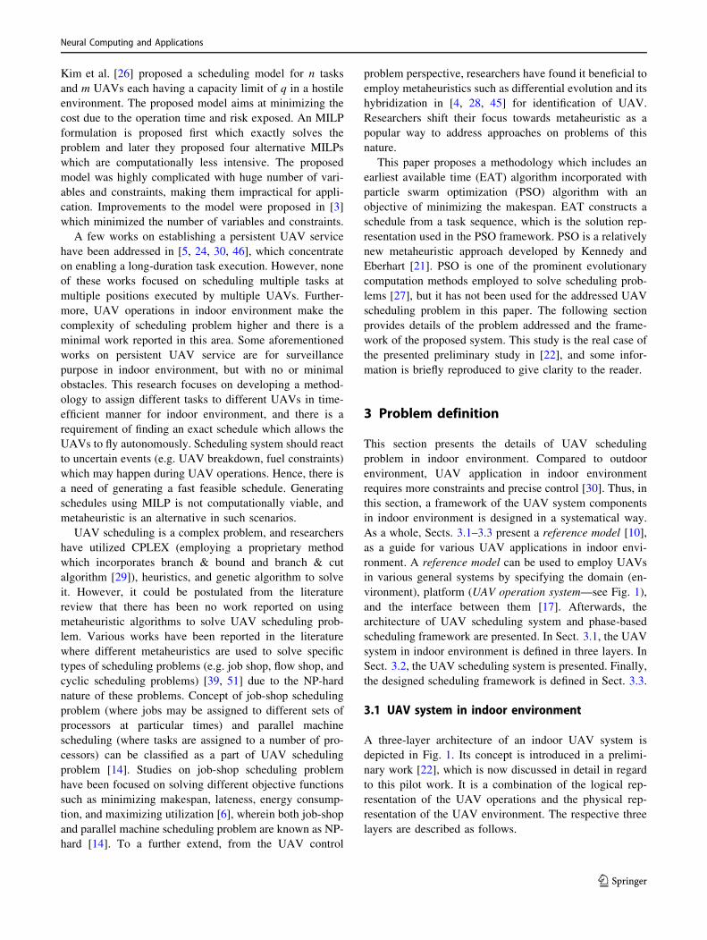
current availability of each task. Table 2 is an example of

the task data. UAV data consist of current state, position,

and battery status of each UAV. Trajectory data used in

phase 1 are built upon the travel time data between posi-

tions in the high-level map. The map is considered as a

complete graph, and all the distances are calculated based

on the shortest path between positions.

Table 3 is an example of the trajectory data containing 6

positions (a–f) and 2 recharge stations (R1, R2), based on

the shortest flight time. This data example is used to

illustrate how the proposed methodology works in Sect. 4.

As the result, a schedule is generated—which comprises

the task executions and other actions assigned to the UAVs.

Scheduler Component

1. Task Data2. UAV Data3. Trajectory Data

Assigning execution timestamp and UAV to tasks

Partial rescheduling

Low-level schedule

High-level schedule with recharging(not considering flight collision avoidance)

Input Information

Phase 1: Assignment phase

Phase 1 Output

Phase 2: Anti-collision refinement phase

Output Information

Fig. 2 Phase-based scheduling framework

Neural Computing and Applications

123

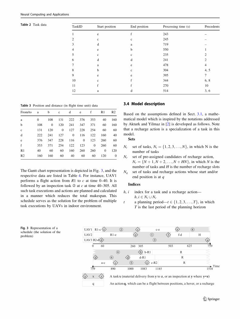
The Gantt chart representation is depicted in Fig. 3, and the

respective data are listed in Table 4. For instance, UAV1

performs a flight action from R1 to c at time 0–40. It is

followed by an inspection task ` at c at time 40–305. All

such task executions and actions are planned and calculated

in a manner which reduces the total makespan. This

schedule serves as the solution for the problem of multiple

task executions by UAVs in indoor environment.

3.4 Model description

Based on the assumptions defined in Sect. 3.1, a mathe-

matical model which is inspired by the notations addressed

by Akturk and Yilmaz in [2] is developed as follows. Note

that a recharge action is a specialization of a task in this

model.

Sets

Nt set of tasks, Nt ¼ f1; 2; 3; . . .;Ng, in which N is the

number of tasks

Nr set of pre-assigned candidates of recharge action,

Nr ¼ fN þ 1;N þ 2; . . .;N þ HNg, in which N is the

number of tasks and H is the number of recharge slots

Nq set of tasks and recharge actions whose start and/or

end position is at q

Indices

h, i index for a task and a recharge action—

h; i 2 Nt [ Nr

t a planning period—t 2 f1; 2; 3; . . .; Tg, in which

T is the last period of the planning horizon

Table 2 Task dataTaskID Start position End position Processing time (s) Precedents

1 e f 243 –

2 c c 245 –

3 d a 719 –

4 e b 550 1

5 c c 235 2

6 d d 241 2

7 a e 478 4

8 b c 304 4, 5

9 e e 395 7

10 c f 344 6, 8

11 f f 270 10

12 a d 514 3, 6

Table 3 Position and distance (in flight time unit) data

From/to a b c d e f R1 R2

a 0 108 131 222 376 353 40 160

b 108 0 120 241 347 371 60 160

c 131 120 0 127 228 254 60 60

d 222 241 127 0 116 122 160 40

e 376 347 228 116 0 123 260 60

f 353 371 254 122 123 0 260 60

R1 40 60 60 160 260 260 0 120

R2 160 160 60 40 60 60 120 0

60 759

R2-d

UAV1UAV2UAV3 d a

R1-e f-d HR1-c c-e

503

e

0

Time

625305

d-R1b-R1

a-c c-R2

RR

R

8151098 10830001957 1185

dd

b

c c

c ce f

260

xy z

q An action q, which can be a flight between positions, a hover, or a recharge

A task x (material delivery from y to z, or an inspection at y where y=z)

Fig. 3 Representation of a

schedule (the solution of the

problem)

Neural Computing and Applications

123

k index for the order of a task executed by a UAV—

k 2 f1; 2; 3; . . .;Kg, in which K is the total number

of tasks executed by a UAV

r index for the order of a recharge action executed by

a UAV—r 2 f1; 2; . . .;Rg, in which R is the latest

index of recharge which is done by a UAV

throughout the planning horizon, and the end time of

the 0th recharge only indicates the beginning of the

planning horizon

u index for a UAV—u 2 f1; 2; 3; . . .;Ug, in which

U is the number of UAVs

p, q index for a position—p; q 2 f1; 2; 3; . . .;Qg, in

which Q is the number of positions

Decision variables

Xiuk ¼ 1 iftaskiisassignedasthek�thtaskofUAVu

0 otherwise

�

Yhi ¼ 1 iftaskhprecedestaskionthesameUAV

0 otherwise

�

Siuk 2 Zþ, start time of task i assigned to UAV u as its k-

th task

Fiuk 2 Zþ, finish time of task i assigned to UAV u as its

k-th task

Ziukr

¼ 1 iftaskiisthek�thtaskandther�threchargeactionofUAVu

0 otherwise

�

Parameters

wi task execution time of task i

Phi ¼ 1 if task h precedes task i

Oi start position of task i

Di end position of task i

dpq distance between position p and q

v0 fixed flight speed of UAV (with or without payload)

C battery capacity—upper bound of the flight time

between battery recharges

Tasks and recharge actions scheduled in the mathe-

matical model consist of two disjoint sets. The first set

called Nt comprises the tasks defined in the task layer in

Sect. 3.1. As mentioned above, three types of task covered

in this study consists of single inspection, compound

inspection, and material handling tasks. Another set called

Nr comprises the recharge actions. The total number of

recharge actions can be the same as the tasks, in the worst

case. Each recharge action can be executed in one of the

recharge slots in multiple recharge stations. Note that a

recharge station may consist of multiple recharge slots. In

the mathematical model, each recharge slot has a unique

position. Correspondingly, the number of the predefined

recharge actions is the product of the number of tasks and

the number of all recharge slots. Unlike tasks, recharge

actions do not have precedence constraint. As mentioned in

the model description, the battery level is conversed in time

dimensional unit.

Decision variable Xiuk, Yhi, Siuk, Fiuk follows the mod-

elling formalism of Akturk and Yilmaz [2]. The extended

model covers the battery constraint and collision avoidance

constraint with additional decision variables Ziukr . Xiuk and

Table 4 Scheduled tasks and

actions in Fig. 3UAV ID Task or action Start position End position Start timestamp End Timestamp

1 R1-c R1 c 0 60

1 2 c c 60 305

1 c–e c e 305 533

1 4 e b 533 1083

1 b-R1 b R1 1083 1143

1 R R1 R1 1143 3843

2 R1-e R1 e 0 260

2 1 e f 260 503

2 f–d f d 503 625

2 H d d 625 759

2 6 d d 759 1000

2 d-R1 d R1 1000 1160

2 R R1 R1 1160 3860

3 R2-d R2 d 0 40

3 3 d a 40 759

3 a–c a c 759 890

3 5 c c 890 1125

3 c-R2 c R2 1125 1185

3 R R2 R2 1185 3885

Neural Computing and Applications

123

Yhi define the task sequence of each UAV. Siuk and Fiuk

define the start time and finish time of each task, respec-

tively. Ziukr discriminates the recharge action from the task

sequence. This leads to the distinction of the consecutive

recharge actions, which is then used to calculate the battery

consumption between recharges. The mathematical model

formulation is given by the following objective function,

Minimize ðmaxi;u;k

FiukÞ 8i 2 Nt [ Nr; 8u; k ð1Þ

subject to

XUu¼1

XKk¼1

Xiuk ¼ 1 8i 2 Nt ð2Þ

XUu¼1

XKk¼1

Xiuk � 1 8i 2 Nr ð3Þ

Xi2Nt[Nr

Xiuk � 1 8u; k ð4Þ

wiXiuk �Fiuk � Siuk 8i 2 Nt [ Nr; 8u; k ð5Þ

Fh;u;k�1 þdDhOi

v0

Yhi � Siuk 8h; i 2 Nt [ Nr; 8u; k ð6Þ

Xh;u;k�1 þ Xiuk � 1� Yhi 8h; i 2 Nt [ Nr; 8u; k ð7Þ

XUu¼1

Xi2Nt[Nr

Xiuk �XUu¼1

Xi2Nt[Nr

Xi;u;k�1 8k ð8Þ

FhvlPhi � Siuk 8h; i 2 Nt; 8q; u; v; k; l ð9Þ

ðShvl � FiukÞðSiuk � FhvlÞ� 0 8h; i 2 Nq; 8q; u; v; k; lð10Þ

Xi2Nr

XKk¼1

SiukZiukr �Xh2Nr

XKl¼1

FhulZh;u;l;r�1 �C 8u; r ð11Þ

XKk¼1

Ziukr � 1 8i 2 Nr; 8u; r ð12Þ

Fiuk �C 1 þXRr¼1

Xkl¼1

Xh2Nr

Zhulr

!8i 2 Nt [ Nr; 8u; k

ð13Þ

The objective of the mathematical model is to minimize the

total makespan of the operations. Constraints (2)–(6) are

featured in Akturk and Yilmaz [2]. Constraint (2) assigns a

task to be executed once by one UAV. Note that constraint

(2) is defined only for tasks, and constraint (3) is defined

for recharge actions. Constraint (4) assures each time slot

of each UAV to be assigned to at most one task or recharge

action. Equation (5) defines the relation between start time

and finish time. Constraints 6 and 7 describe the task

sequence and the time relation between tasks.

Constraint (8) is provided for the strictness of the mathe-

matical model. It prevents empty slots in the middle of the

time slot sequence of each UAV, which causes the asso-

ciated decision variables Yhi, Siuk, Fiuk, and Ziukr undefined.

Constraint (9) defines the precedence constraint, and con-

straint (10) defines the position occupation constraint in a

nonlinear form. The constraint assures that any pair of two

tasks cannot be executed simultaneously. Constraint (11)

describes the battery constraint in a nonlinear form. The

time gap between every consecutive recharge action is

restricted to be less than the battery capacity. It enforces

the necessary amount of recharge actions accordingly.

Constraint (12) is an assignment constraint making the

relation between the task sequence and the recharge

sequence of each UAV. Constraint (13) is a bin-packing-

like constraint [41] for each UAV to schedule at least a

minimum required number of recharges—assuming that

the UAVs are fully charged in the beginning of the plan-

ning horizon.

In regard to the considered constraints, the problem in

this paper draws an input from parallel machine scheduling

(PMS) problem [37]. Since multiple tasks can be executed

by multiple available UAVs, the UAVs can be analogized

to parallel machines. The proposed problem covers the one

which is preliminarily defined in [32], which is investigated

under the constraint satisfaction programming (CSP)

modelling formalism. PMS problem is one of the most

reported works in the scheduling literature [12]. Garey and

Johnson [15] showed that PMS problems with the objective

of minimizing the makespan are categorized as NP-hard.

One constraint of the addressed problem is that the tasks

which are assigned to the same position cannot be executed

simultaneously. Under this constraint, not only the UAVs,

but also the positions should be considered as resources.

Several researchers have studied various scheduling prob-

lems with different constraints. Kellerer and Strusevisch

[20] showed that the two-machine problem with one

additional resource type is NP-hard. Hou and Guo [19]

proposed an MIP model of parallel machine scheduling

with resource constraints and sequence-dependent setup

times, which was also reported to be NP-hard. Another

crucial constraint of the addressed problem is the capaci-

tated battery constraint. It inflicts necessary UAV recharges

which proportionally depend on the execution of the

assigned tasks. From the classic scheduling problem, this

issue has been discussed as a preventive maintenance

problem. Qi et al. [35] proved that the maintenance

scheduling on a single machine is NP-hard problem by

reducing it to distance-constrained VRP (vehicle routing

problem). Xu et al. [49] modelled parallel machine

scheduling with �-almost periodic maintenance constraint,

which means that the time between any two consecutive

maintenance is within the interval ½T ; T 0�, where T and T 0

Neural Computing and Applications

123

are positive real numbers and T 0 � T\�. Consequently, it

can be concluded that the nature of the addressed problem

in this paper is also NP-hard.

There are various possible objectives which can be

considered in the UAV scheduling problem, as in various

other scheduling problems. Among different objectives

[34, 40], minimization of makespan is selected to be

optimized in this paper. A makespan indicates the general

throughput of the UAV scheduling system, and an opti-

mized makespan means an efficient UAV schedule which

maximizes this throughput where tasks are executed in a

time-efficient manner. It can also be considered as a

measure of the battery consumption and resource utiliza-

tion. To achieve this objective, a proposed heuristic is

incorporated with particle swarm optimization (PSO)

algorithm which will be discussed in the following section.

4 Application of PSO for UAV schedulingsystem

Characteristics of the presented problem distinguish its

nature as NP-hard. Approaches based on branch & bound

and branch & cut are tedious in terms of computation time.

A promising alternative to those methods is a metaheuristic

algorithm. Metaheuristics use different concepts derived

from artificial intelligence and evolutionary algorithms,

which are inspired from mechanisms of natural evolution

[40]. From the literature, it could be found that meta-

heuristics can also be called as soft computing techniques,

evolutionary algorithms, and nature-inspired algorithms.

Metaheuristic methods are designed for solving a wide

range of hard optimization problems without having to

adapt deeply into each problem. These algorithms are fast

and easy to implement [44]. From the literature review, it

could be seen that different metaheuristic algorithms have

been proposed to obtain feasible solutions for general

scheduling problems [16].

Particle swarm optimization (PSO) algorithm is a

swarm-based stochastic optimization technique developed

by Kennedy and Eberhart [21] based on the characteristics

of social behaviour of birds in flocks or fish in schools. This

metaheuristic algorithm is chosen to be incorporated in the

proposed methodology in this paper. PSO algorithm does

not involve the usage of genetic operators (mutation and

crossover) which are commonly used for evolutionary

algorithms. On top of that, PSO utilizes a minimum num-

ber of parameters to achieve the near-optimum solution in a

faster computation time [31]. These factors have influenced

the authors to choose PSO to solve the presented problem,

where there is a requirement of generating a fast and fea-

sible schedule in a real-time application.

PSO is an optimization method based on the population

which is referred as swarm in this paper. Simplicity in

application, easy implementation, and faster convergence

of PSO have made the algorithm widely acceptable among

researchers for solving different types of optimization

problem [18]. Different variants of PSO have been devel-

oped and employed by researchers to solve scheduling

problems. This paper employs the standard PSO [21]

model to solve the UAV scheduling problem. The pseu-

docode of PSO is presented in Algorithm 1. All particles in

the swarm share the global best particle information which

helps to search towards the best position in the search

space. Each single solution in the search space is called as a

particle. All particles are to be evaluated by an objective

function (explained in the following section) which is to be

optimized. Each particle in the swarm searches for the best

position, and it travels in the search space with a certain

velocity. Best fitness encountered by each particle (local

best) is stored and the information is shared with other

particles to obtain the best particle (global best). In this

paper, the velocity and position update of PSO are based on

[36] to suit the presented UAV scheduling problem.

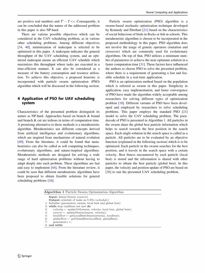
Algorithm 1 Particle Swarm Optimization AlgorithmInput: Initial Swarm (swarm)Output: schedule of tasks on UAVs (schedule)

1: Initialize (parameters, swarm, local best and global best)2: while stop condition not met do3: velocity ← updateVel(swarm, velocity, local best, global best);4: swarm ← updateSwarm(swarm, velocity);5: localBest ← getLocalBest(fitness(swarm), localbest);6: globalBest ← getGlobalBest(localBest, globalBest);7: generation++;8: end while

Neural Computing and Applications

123

The procedural steps of the PSO algorithm are given

below:

Step 1 The initial population is generated based on

priority rules. Initial velocities for each particle

are randomly generated.

Step 2 Based on the objective function, each particle is

evaluated.

Step 3 Each particle remembers the best result achieved

so far (local best) and exchange information with

other particles to obtain the best particle (global

best) among the swarm.

Step 4 The velocity of the particle is updated using

Eq. (14), and the position of the particle is

updated using Eq. (15).

Velocity update equation:

vtþ1i ¼vtiþc1� U1� loPt

i�Pti

� �� �|fflfflfflfflfflfflfflfflfflfflfflfflfflfflfflffl{zfflfflfflfflfflfflfflfflfflfflfflfflfflfflfflffl}cognitivepartþc2� U2� Gt�Pt

i

� �� �|fflfflfflfflfflfflfflfflfflfflfflfflfflfflffl{zfflfflfflfflfflfflfflfflfflfflfflfflfflfflffl}socialpart

ð14Þ

where U1 andU2 are known as velocity coefficients (random

numbers between 0 and 1), c1 and c2 are known as learning

(or acceleration) coefficients, vti is the initial velocity (which

comprises pairs of transposition—see Sect. 4.1.2), loPti is the

local best,Gt is the global best solution at generation t, andPti

is the current particle position.

Acceleration coefficients c1 and c2 are the important

parameters of PSO. Parameter c1 is used to guide the particle

towards its own (local) best position, and this behaviour

enhances the grouping ability and keeps the diversity of the

population. Parameter c2 acts as a convergence factor that

attracts all the particles towards the global best position.

To suit the considered problem, the particle is repre-

sented in the form of a task sequence (for an example, refer

the value of particle in Table 5). This enables a

tractable update during the numerous iterations. A particle

represents a feasible solution which consists of a sequence

of tasks. The sequence shall satisfy the precedence rela-

tionships, and it is initially generated based on a priority

rule. The priority rules which are considered in this study

are explained in Sect. 4.1.1. A velocity of a particle is a

collection of transpositions, where each transposition is

represented as position indices of two tasks in a sequence

(particle) which will be swapped accordingly (during the

velocity update). In this study, the position index starts

from 0 instead of 1 for a seamless implementation (from

the programming perspective).

Each particle changes its position according to its

velocity, which is randomly generated towards the local

best (loPti) and the global best (Gt) positions. The moving

direction of the particle is decided by three parts as shown

in Eq. (14). These three parts comprise the initial velocity

vti of the particle at a particular iteration, the optimum

distance of loPti � Pt

i that the particle passed (this is known

as a cognitive part which controls the exploration of the

particle based on its own exploration experience), and the

optimum distance of Gt � Pti that the particle swarm passed

(this is known as a social part which helps in collaborating

with other particles based on the group exploration expe-

rience [7]). The proportions of impact for cognitive and

social parts are decided based on the coefficients c1 and c2.

These coefficients determine whether a particle prefers to

move closer to the local best or global best position.

A particle moves from its current position to the new

position using Eq. (15). The position of every particle in

the swarm is updated in every iteration.

Position update equation:

Ptþ1i ¼ Pt

i þ vtþ1i ð15Þ

Different operators used in computing the particle velocity

and position are explained as follows [36].

– Subtraction (position–position) operator Let two

positions x1 and x2 represent two different task

sequences (see Sect. 4.1.1). The difference of x2 � x1

is a velocity v. In Eq. (14), subtracting two positions,

i.e. loPti � Pt

i results in a velocity which is a set of

transpositions (see Sect. 4.1.2). The difference of the

positions of two particles can be obtained in various

implementation ways. For instance, each element

Table 5 Example data and

parameters for PSO procedureData or parameter Notation Value

Local best particle loPti

[1, 2, 4, 6, 5, 8, 3, 7, 10, 9, 11, 12]

Global best particle Gt [2, 6, 1, 4, 3, 5, 7, 8, 10, 9, 11, 12]

Particle Pti [1, 2, 4, 6, 5, 8, 7, 3, 10, 9, 12, 11]

Initial velocity vti (6, 7), (10, 11)

Learning coefficient 1 c1 1

Learning coefficient 2 c2 2

Velocity coefficient U1 0.2

Velocity coefficient U2 0.4

Neural Computing and Applications

123

(A) in the first particle is compared with element (B) in

the second particle at the same position index. When

they are different, the position of B is searched in the

first particle. That position index is then coupled with

the position index of A. After completing all iterations,

a collection of position index pairs (for performing a

transposition) is obtained. This procedure has been

widely used in [31, 36].

– Addition (position 1 velocity) operator Let x1 be a

position, and v be a velocity of the particle. New

position x2 is calculated by applying each transposition

pair in v consecutively to x1.

– Addition (velocity 1 velocity) operator Let v1 and v2

be two velocities (which may come from either one of

the three parts of Eq. (14)). In order to calculate

v1 þ v2, the list of transpositions combines the subsets

of transpositions from v1 and v2.

– Multiplication (constant * velocity) operator Let c be

a constant and v be a velocity (which consists of one or

more transposition pairs). The operation of c � v results

in a new velocity with an equal or less number of

transposition pairs, where the first c � 100% proportion

of the collection is selected.

Step 5 Go back to step 2 until the termination criterion is

met. Equations (14) and (15) describe the path in which the

particles move in the search space.

In this paper, PSO is used to optimize the proposed

problem, where one of the key challenges encountered is

the encoding of the particle. In most applications of PSO,

particle position Pti is directly denoted as the solution in the

form of a sequence of tasks. The arrangement of the

sequence is ensured to satisfy the precedence relationships.

To illustrate how the velocity and position update work, an

example is explained as follows—the notations of the

required data or parameters are depicted in Table 5.

The current velocity of a particle is updated based on

Equation (14) as follows.

vtþ1i ¼ ð6; 7Þð10; 11Þ þ 0:2 �

½ð1; 2; 4; 6; 5; 8; 3; 7; 10; 9; 11; 12Þ� ð1; 2; 4; 6; 5; 8; 7; 3; 10; 9; 12; 11Þ�þ 0:8 � ½ð2; 6; 1; 4; 3; 5; 7; 8; 10; 9; 11; 12Þ� ð1; 2; 4; 6; 5; 8; 7; 3; 10; 9; 12; 11Þ�¼ ð6; 7Þð10; 11Þ þ 0:2 � ð6; 7Þð10; 11Þþ 0:8 � ð0; 1Þð1; 3Þð2; 3Þð4; 7Þð5; 7Þð10; 11Þ

¼ð6; 7Þð10; 11Þð0; 1Þð1; 3Þð2; 3Þð4; 7Þð5; 7Þ

Using Eq. (15), the current particle is updated to a new

particle using the new velocity.

Ptþ1i ¼ ð1; 2; 4; 6; 5; 8; 7; 3; 10; 9; 12; 11Þ

þ ð6; 7Þð10; 11Þð0; 1Þð1; 3Þð2; 3Þð4; 7Þð5; 7Þ¼ ð2; 6; 1; 4; 7; 5; 3; 8; 10; 9; 11; 12Þ

The products of coefficient values c1, U1 and c2, U2 rep-

resent the proportion which decides how many pairs of

transposition would be copied to form the updated velocity.

For example, when the proportion is 80%

(c2 � U2 ¼ 2 � 0:4 ¼ 0:8), 80% of the pairs would be

copied to the updated velocity. In this example, 6 pairs are

formed when transpositions take place between the global

best and the current particle. Based on this proportion, 5

pairs are chosen out of 6 for the updated velocity. How-

ever, if any of the pairs is already present from other

transpositions or initial velocity, it is discarded. A repair

mechanism is incorporated to convert an infeasible

sequence to a feasible one which meets the precedence

relationships—presented as Algorithm 3 in this paper.

4.1 PSO entities

To illustrate the explanation of different entities in PSO, a

sample dataset presented in Tables 2 and 3 is used.

4.1.1 Initial population

Metaheuristic algorithms start with a random search state

which iteratively evolves to find a near-optimum solution

[34]. Despite the search state being random, the generation

of the initial population is not purely random but guided by

the priority (heuristic) rules. The purpose for doing this is

to start the search from hypothetically good starting points

rather than random ones, so that global optimum is more

likely achieved in less computation time. In this paper, six

priority rules (maximum rank positional weight, minimum

inverse positional weight, minimum total number of pre-

decessor tasks, maximum total number of follower tasks,

maximum and minimum task time) presented in [34] are

used to generate the initial particles. Two more priority

rules based on the number of predecessor and follower

tasks are added to the existing rules, and these are named as

cumulative number of predecessor and follower tasks.

Based on these eight priority rules, eight initial particles

can be generated respectively. In regard to the number of

initial particles, it is reported in the literature that a high

initial population size improves the quality of the solution.

Hence, up to forty initial particles are generated in the

experiments. Each remaining particle apart from the

aforementioned eight is generated by randomly swapping

the tasks in one of the eight particles without violating the

precedence relationships and produces a new one. Table 6

reports the set of initial particles generated using the

Neural Computing and Applications

123

priority rules and conformed with Algorithm 3 to satisfy

the precedence relationships. The precedence relationships

of tasks are available in Table 2. Each particle is structured

as a string of tasks which are to be executed in the UAV

operation.

4.1.2 Initial velocity

Each particle is assigned with velocity pairs, and these

pairs are randomly generated. Based on the pilot experi-

ments, it is decided to have different sizes of velocity pairs

for different problems based on the number of tasks.

Table 7 presents the maximum number of velocity pairs

used in this research for different numbers of task. The

velocity is updated from the second iteration using

Eq. (14). The number of pairs is the same throughout all

iterations. For example, if the number of tasks is within the

range of 0–20, the number of velocity pairs is selected as 2.

4.2 Schedule creation and evaluation

In the addressed methodology, the initial population is

generated according to the priority rules explained in

Table 6. Tasks in the task sequence are scheduled, where

each of them is assigned to a UAV to be executed in a

particular timespan, one by one (per step) according to its

order in the sequence. Figure 4 depicts the sequential steps

of creating a schedule from a sequence of 12 tasks.

The aforementioned heuristic for creating a schedule

from a task sequence is depicted in Algorithm 2. The idea

behind this algorithm is to create a schedule which is dri-

ven to utilize the available resources in the following

manners, which generally lead to a time-efficient

characteristic:

– balanced

– task assignment towards the earliest available UAV

(which indicates its relative idleness compared to

other UAVs)

– safe

– no multiple UAVs are allowed to occupy a position

simultaneously

– task execution follows the precedence relationship

– early

– recharge station which eventually delivers a

recharged UAV to its next destination early is

chosen

– the shortest makespan found during the search is

selected as the final solution

The detailed procedure of the heuristic is explained in

Algorithm 2.

Table 6 Priority rules for initial

swarm generationPriority rules Task sequence (generated particle)

Maximum ranked positional weight 1 2 4 6 5 8 3 7 10 9 11 12

Minimum inverse positional weight 1 2 3 4 5 6 7 12 9 8 10 11

Minimum total number of predecessors tasks 1 2 3 4 5 6 7 9 8 10 11 12

Maximum total number of follower tasks 2 6 1 4 3 5 7 8 10 9 11 12

Maximum task execution time 3 2 1 4 7 9 6 12 5 8 10 11

Minimum task execution time 1 2 5 6 4 8 10 11 7 9 3 12

Minimum number of cumulative predecessor

tasks

1 2 3 4 5 6 7 9 12 8 10 11

Maximum number of cumulative follower tasks 1 2 4 5 6 8 3 7 10 9 11 12

Table 7 Number of initial velocity pairs in regard to the number of

tasks

Number of tasks Maximum number of velocity pairs

0–20 2

20–50 10

50–100 30

Neural Computing and Applications

123

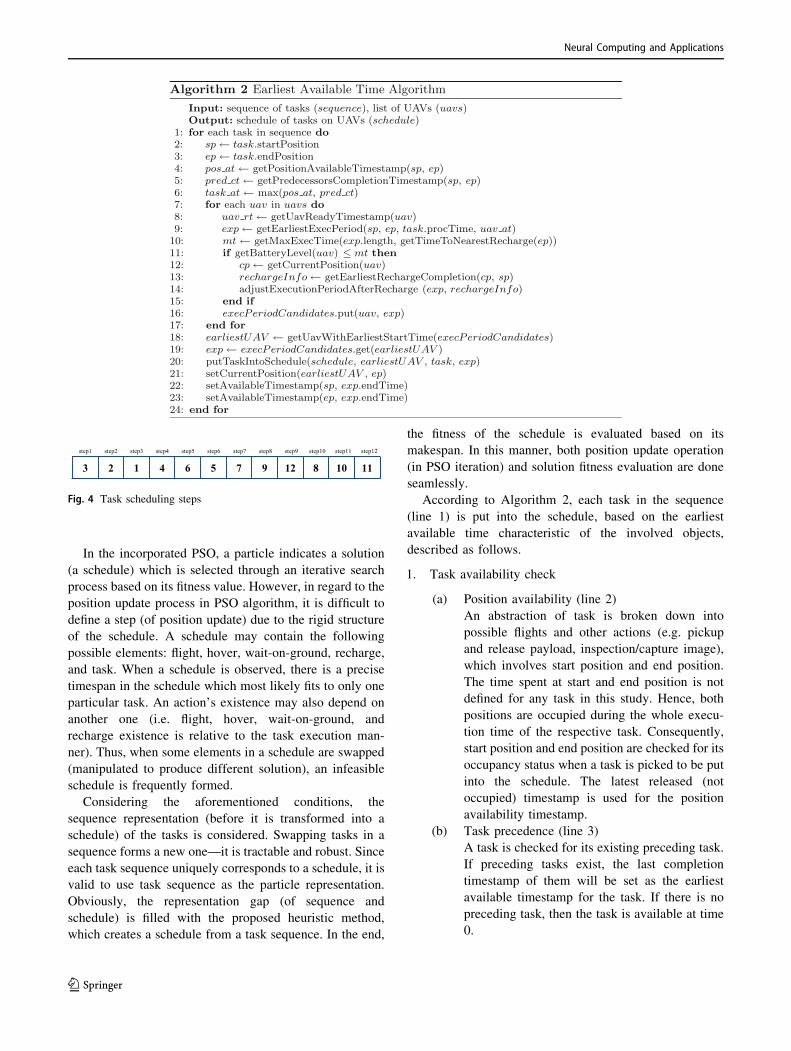
Algorithm 2 Earliest Available Time AlgorithmInput: sequence of tasks (sequence), list of UAVs (uavs)Output: schedule of tasks on UAVs (schedule)

1: for each task in sequence do2: sp ← task.startPosition3: ep ← task.endPosition4: pos at ← getPositionAvailableTimestamp(sp, ep)5: pred ct ← getPredecessorsCompletionTimestamp(sp, ep)6: task at ← max(pos at, pred ct)7: for each uav in uavs do8: uav rt ← getUavReadyTimestamp(uav)9: exp ← getEarliestExecPeriod(sp, ep, task.procTime, uav at)10: mt ← getMaxExecTime(exp.length, getTimeToNearestRecharge(ep))11: if getBatteryLevel(uav) ≤ mt then12: cp ← getCurrentPosition(uav)13: rechargeInfo ← getEarliestRechargeCompletion(cp, sp)14: adjustExecutionPeriodAfterRecharge (exp, rechargeInfo)15: end if16: execPeriodCandidates.put(uav, exp)17: end for18: earliestUAV ← getUavWithEarliestStartTime(execPeriodCandidates)19: exp ← execPeriodCandidates.get(earliestUAV )20: putTaskIntoSchedule(schedule, earliestUAV , task, exp)21: setCurrentPosition(earliestUAV , ep)22: setAvailableTimestamp(sp, exp.endTime)23: setAvailableTimestamp(ep, exp.endTime)24: end for

In the incorporated PSO, a particle indicates a solution

(a schedule) which is selected through an iterative search

process based on its fitness value. However, in regard to the

position update process in PSO algorithm, it is difficult to

define a step (of position update) due to the rigid structure

of the schedule. A schedule may contain the following

possible elements: flight, hover, wait-on-ground, recharge,

and task. When a schedule is observed, there is a precise

timespan in the schedule which most likely fits to only one

particular task. An action’s existence may also depend on

another one (i.e. flight, hover, wait-on-ground, and

recharge existence is relative to the task execution man-

ner). Thus, when some elements in a schedule are swapped

(manipulated to produce different solution), an infeasible

schedule is frequently formed.

Considering the aforementioned conditions, the

sequence representation (before it is transformed into a

schedule) of the tasks is considered. Swapping tasks in a

sequence forms a new one—it is tractable and robust. Since

each task sequence uniquely corresponds to a schedule, it is

valid to use task sequence as the particle representation.

Obviously, the representation gap (of sequence and

schedule) is filled with the proposed heuristic method,

which creates a schedule from a task sequence. In the end,

the fitness of the schedule is evaluated based on its

makespan. In this manner, both position update operation

(in PSO iteration) and solution fitness evaluation are done

seamlessly.

According to Algorithm 2, each task in the sequence

(line 1) is put into the schedule, based on the earliest

available time characteristic of the involved objects,

described as follows.

1. Task availability check

(a) Position availability (line 2)

An abstraction of task is broken down into

possible flights and other actions (e.g. pickup

and release payload, inspection/capture image),

which involves start position and end position.

The time spent at start and end position is not

defined for any task in this study. Hence, both

positions are occupied during the whole execu-

tion time of the respective task. Consequently,

start position and end position are checked for its

occupancy status when a task is picked to be put

into the schedule. The latest released (not

occupied) timestamp is used for the position

availability timestamp.

(b) Task precedence (line 3)

A task is checked for its existing preceding task.

If preceding tasks exist, the last completion

timestamp of them will be set as the earliest

available timestamp for the task. If there is no

preceding task, then the task is available at time

0.

step1 step2 step3 step4 step5 step6 step7 step8 step9 step10 step11 step12

3 2 1 4 6 5 7 9 12 8 10 11

Fig. 4 Task scheduling steps

Neural Computing and Applications

123

2. UAV availability check

(a) UAV ready time (8)

Task occupancy of each UAV is checked. The

moment it goes to idle after completing the most

recent task is recorded as its ready time.

(b) Battery level (lines 10–11)

After a task execution, a UAV must have

enough battery level to at least fly towards the

nearest recharge station.

(c) Recharge time (lines 10–15)

The battery check which is done in the part of

line 10 is done to guarantee a sufficient battery

level to go to at least the nearest recharge

station. If a UAV doesn’t have enough battery to

go to the recharge station after executing a task,

then it needs to go to the recharge station with

the earliest recharge completion time before

flying to the start position of the task and

execute it. To ensure that the UAV is fully

charged (at a capacity of 1200 s flight), an actual

recharge timespan is always set to 2700 s; it is

the time required to do a full battery recharge.

Recharge time is the summation of round-trip

time and actual recharging timespan (which may

be longer than 2700 s due to the delayed

recharge station availability time).

(d) Recharge station availability (line 13)

A limited number of recharge slots at the

recharge station are considered. When all

recharge slots at a recharge station are occupied,

its earliest available time is the earliest times-

tamp when an occupying UAV leaves the

recharge station. The next selection criteria is

based on the shortest round-trip (end position of

previous task ! recharge station ! start

position of current task) time to a recharge

station. It means that the nearest recharge station

might not be preferred due to its far distance to

the start position of the current task.

3. Overall availability check (lines 4–18)

Incorporating the aforementioned task availability and

UAV availability check, the start timestamp of the

respective task is calculated. A UAV with the earliest

overall available time is selected (line 18), and the task

is put into the respective UAV’s schedule. Completion

(end) timestamp of a task potentially performed by

each UAV is also included in the execution period

calculation (line 9) and used to release the occupied

positions (lines 22–23).

For readability, putTaskIntoSchedule (line 24) in Algo-

rithm 2 encapsulates the following processes:

1. Insert a task into the schedule of the selected (earliest

available) UAV

2. Insert a recharge action (if required) into the schedule

of the selected UAV

(a) update occupancy status of the respective

recharge slot

3. Update battery level of the respective UAV

4. Insert hover and wait-on-ground in between tasks in

the schedule when needed

These supplementary actions are required to generate a

feasible schedule of UAV operations [22].

To illustrate the usage of the heuristic described in Algo-

rithm 2, steps 1–7 of the task scheduling process for a given

task sequence in Fig. 4 are presented. Steps 1 and 2 are

depicted in Figs. 5 and 6, while steps 3–7 are presented in

‘‘Appendix A’’. Steps 8–12 which are principally doing the

same procedure as the previous ones are not presented in

the paper. In accordance with the explanation of Algorithm

2, task and UAV availability check are performed every

time a task is picked to be put into the schedule. Detailed

stepwise procedure for the first two steps is explained

below the figures. Task, UAV, and overall availability

check are referred as point (a), (b), and (c), respectively.

After completing all 12 steps, a schedule of 12 task

executions is obtained. The schedule has a makespan of

4963 s, which is called as fitness value of the particle (in

the incorporated PSO).

Furthermore, when there is an infeasible sequence

(which doesn’t meet the precedence relationships) during

the position update, a repair mechanism is conducted based

on Algorithm 3.

Neural Computing and Applications

123

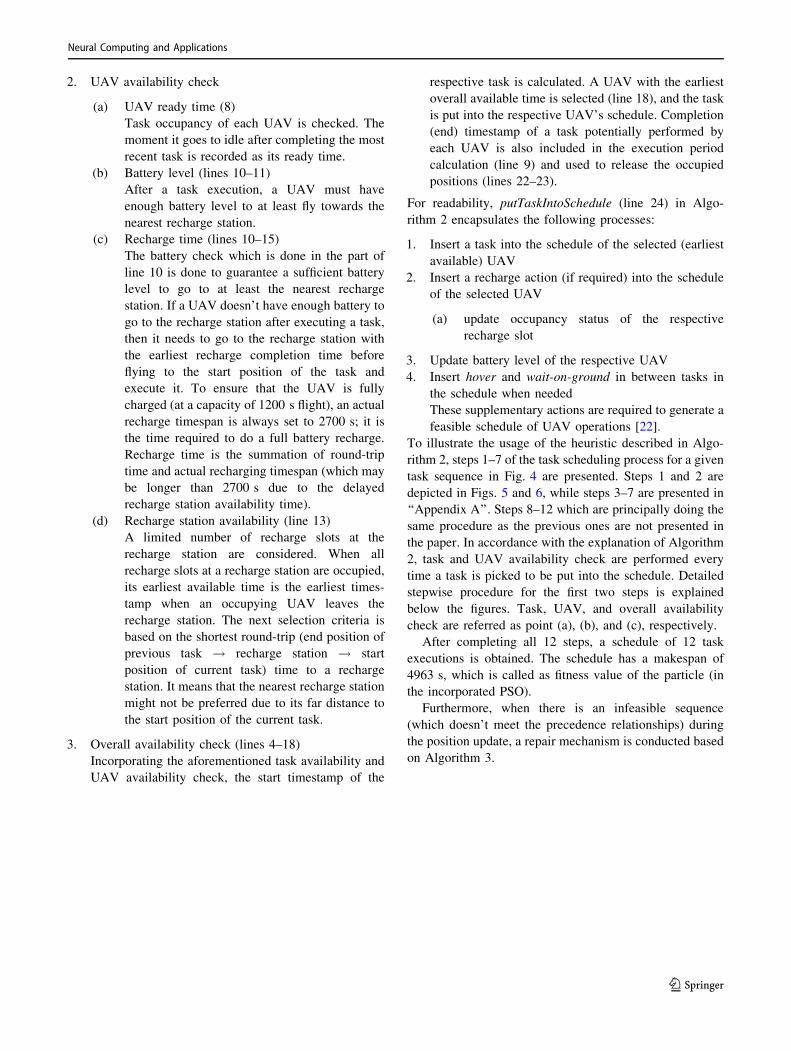
The process can be pictured as moving the tasks from a

sequence to a new one where precedence feasibility is held

along the way. An agent visits the tasks in the task

sequence sequentially as long as there is at least one task in

the original sequence (lines 1–2). It checks each prede-

cessor in the (immediate) predecessor list of the currently

visited task. If it is contained in the new sequence, then it

shall be removed from the list (lines 3–10). If the list of

predecessors of the currently visited task is empty, then this

task is ready to be moved into the new sequence (lines

11–15)—the task is added at the end of the sequence (line

12). Otherwise, it searches the following tasks (according

to the sequence) to find a task which is ready to be moved

(line 2). In the end, a feasible sequence that meets the

precedence relationships is produced, which represents one

valid particle in the PSO framework.

The sample data (Tables 2 and 3) being used in this

section bring an example of task dataset which strongly

displays the logic of Algorithm 2. For further analysis and

evaluation, several datasets with different data volumes are

generated. Respectively, the mechanism of generating the

data is also presented in the following section.

5 Numerical experiments

To examine the behaviour and the performance of the

proposed methodology, numerical experiments are con-

ducted based on 3 task datasets. Several different

treatments are given during those experiments and

explained in detail in Sects. 5.2.1 and 5.2.2. The proposed

algorithm is coded on a Java platform, and the numerical

experiments are conducted on an Intel Core i7 processor

(2.9 GHz) with 32 GB of RAM.

5.1 Data generation

Task dataset used in the experiment is generated based on a

test flight conducted in the laboratory. It is conducted to

measure the speed of the UAV movement in a real-world

indoor environment. Based on the required test case

described in task layer (see Sect. 3.1), several types of task

are classified in Table 8. A single inspection task captures

an observation image of a certain area of interest; its pro-

cessing time is 20–80 s. A compound inspection task

captures multiple observation images of several areas of

interest; its processing time is 100–200 s. Unlike a single

inspection task, compound inspection task might contain

flight actions between captures. Without such an abstrac-

tion, the level of detail will cause a high number of steps in

a solution, which obviously affects the computation time in

finding one. The next type of task is material handling.

Material handling consists of pickup, transport flight, and

release. Its processing time is 30 s for each pickup and

release (30 þ 30 ¼ 60s), while transport flight varies

according to the origin and destination positions.

During the scheduling process, a task has five attributes

attached: task identifier, origin position, destination

40 759

R2-d

UAV1UAV2UAV3 d a

0 Time

Fig. 5 Output of step 1 of the

schedule creation heuristic

Algorithm 3 Task Sequence Repair AlgorithmInput: sequence of tasks (seq)Output: feasible sequence of tasks on UAVs (fseq)

1: fseq ← null2: while seq is not empty do3: for task in seq do4: for d in fseq do5: if task.predecessorList contains d then6: remove d from task.predecessors7: end if8: if task.predecessorList is empty then9: break10: end if11: end for12: if task.predecessorList is empty then13: add task into fseq14: remove task from seq15: break16: end if17: end for18: end while

Neural Computing and Applications

123

Step Description1 Task 3

(a) Task availability checkTask 3 is started at position d, position d is available from time 0.· Task precedenceTask 3 has no precedence and position d is currently available from time 0.

Hence, task 3 is available from time 0.

(b) UAV availability check· UAV ready time (rt)UAV1, UAV2, and UAV3 are ready (not performing any task) from time 0.UAV1: 0; UAV2: 0; UAV3: 0· Battery level & rechargeBattery consumption for task execution is calculatedIt includes flight towards start position (s), task processing time (pt),and flight towards nearest recharge station (rs).UAV x : [rt] + [s] + [pt] + [rs]UAV1 : 0+160+719+40 = 200UAV2 : 0+160+719+40 = 200UAV3 : 0+40+719+40 = 80Note: if the sum of UAV ready time and flight towards start position isless than task availability time, then they are replaced with it.UAV1, UAV2, and UAV3 do not need any recharge because each batteryconsumption is still <1200.If recharge is required, then it will search a recharge station with theshortest round-trip flight.

(c) Overall availability checkUAV1 : 0+60 = 60UAV2 : 0+60 = 60UAV3 : 0+40 = 40∴ UAV3 is selected for task 3.

40 759305

R2-d

UAV1

UAV2

UAV3 d a

R1-c

0Time

c c

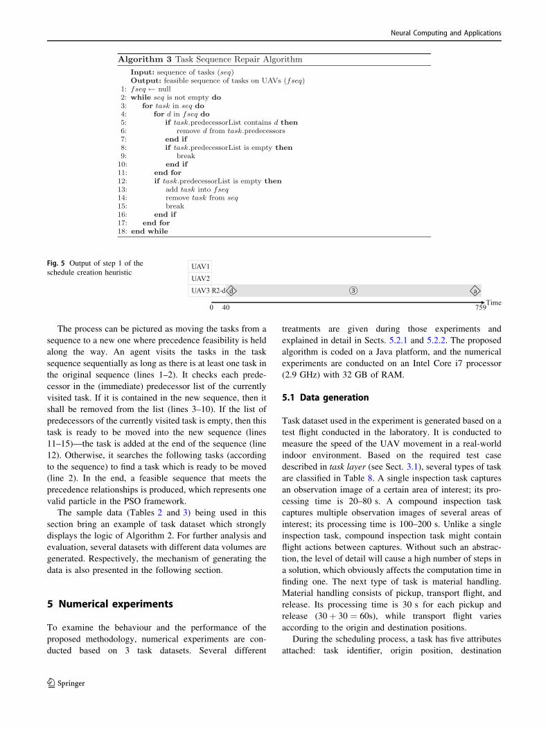
Step Description2 Task 2

(a) Task availability checkTask 2 is available from time 0.

(b) UAV availability checkUAV1 : 0+60+245+60 = 365UAV2 : 0+60+245+60 = 365UAV3 : 759+131+245+60 = 1195No UAV needs recharge.

(c) Overall availability checkUAV1 : 0+60 = 60UAV2 : 0+60 = 60UAV3 : 759+131 = 890∴ UAV1 is selected for task 2.

Fig. 6 Output of step 2 of the

schedule creation heuristic

Neural Computing and Applications

123

position, processing time, and predecessor list (see

Table 9). Task identifier is represented as a unique integer

value, which means that no multiple tasks share the same

value. Origin position and destination position are repre-

sented as a unique string each, which acts as a position

name and a position identifier simultaneously. Processing

time is represented as an integer value where its execution

time shall never exceed the battery capacity of the UAV

(Eq. (16)). Predecessor list is represented as a set of inte-

gers which indicates the identifiers of the preceding tasks.

execution time ¼preparation flight þ processing time

þ towards recharge flight

execution time�UAV BATTERY CAPACITY

ð16Þ

5.2 Parameter analysis and performanceevaluation

In the proposed method, the granularity of the processed

data can be seen as a sequence. From a particular sequence,

a schedule is created using a heuristic based on the pro-

posed earliest available time algorithm. The schedule is

then evaluated through its makespan (the total time

required for completing all tasks based on a schedule). The

process is done iteratively and executed in a manner

according to the PSO algorithm. To control the perfor-

mance of this PSO algorithm, i.e. tendency of optimality

level and convergence speed, a set of parameters need to be

configured. Through the conducted experiments, the

respective performance of each set of parameters is mea-

sured and evaluated in Sect. 5.2.2 to decide the default

parameter values which most likely bring the best result in

regard to the task datasets.

In Sect. 5.2.1, the following parameters are analysed:

1. Size of initial population

Initial particles in the initial population serve as the

initial starting points of the search. The more varying

the starting points are, spread at different locations

throughout the search space, the better chance the

search has in reaching the global optimum instead of

getting trapped at a local one.

2. Number of pairs in initial velocity

To cover a sufficient exploration area of the respective

solution search space, one must adjust the number of

pairs along with the escalation of the number of tasks.

By doing so, a particle is capable to explore its

surrounding search space and more likely to find a

local best particle in that area. In the other way around,

a lower number of pairs in initial velocity minimize the

local exploration and force the search to rely more on

the variety of particles in the initial swarm alone.

3. Value of learning coefficients (c1 and c2) and velocity

coefficients (U1 and U2)

According to Eq. (14) for velocity update, U1 and U2

are fraction numbers randomly generated ranging from

0.0 to 1.0. Furthermore, because of c1 and c2 multi-

plied, respectively, with U1 and U2, they will control

the search direction. c1U1 and c2U2 will decide the

number of pairs used from the distance of the current

particle towards the local and global best particle,

respectively. Since constant c1 is set to be smaller than

constant c2, there will be a tendency of getting more

pairs produced from the social part—from the global

Table 8 Task types

Task type Processing time (s)

Single inspection 20–80

Compound inspection 100–200

Material handling 60 þ flight_time

Table 9 Task attributes

Attribute Data type

Task identifier Integer

Origin position String

Destination position String

Processing time Integer

Predecessor list Integers0 10 20 30 40 50 60

3050

031

000

3150

032

000

n − th run

Mak

espa

n (s

econ

d)

c1 =1, c2 =1c1 =1, c2 =2c1 =2, c2 =1c1 =2, c2 =2

Fig. 7 Overall makespans on 100 tasks

Neural Computing and Applications

123

best sequence. Consequently, all particles in the swarm

are alerted and encouraged to move towards the global

best particle, while being less encouraged to move

towards its own self-obtained local best particle. The

movement of all particles towards the global best

particle indicates the action of convergence during the

whole search process, while the movement of each

particle towards its local best particle allows the swarm

to still explore towards various other directions to get

potentially better global best particle.

5.2.1 Parameter analysis

Three different task datasets are used in the experiment,

each consists of 12, 50 and 100 tasks, operated by 3 UAVs.

In the experiments, makespans of the generated schedules

based on various combinations of parameters: c1, c2, and

initial population size on 3 different task datasets are

measured. Further details can be seen in Fig. 13 in

Appendix, whose summary is representatively depicted in

Fig. 7. Systematically, the granularity of the experimental

run is explained as follows.

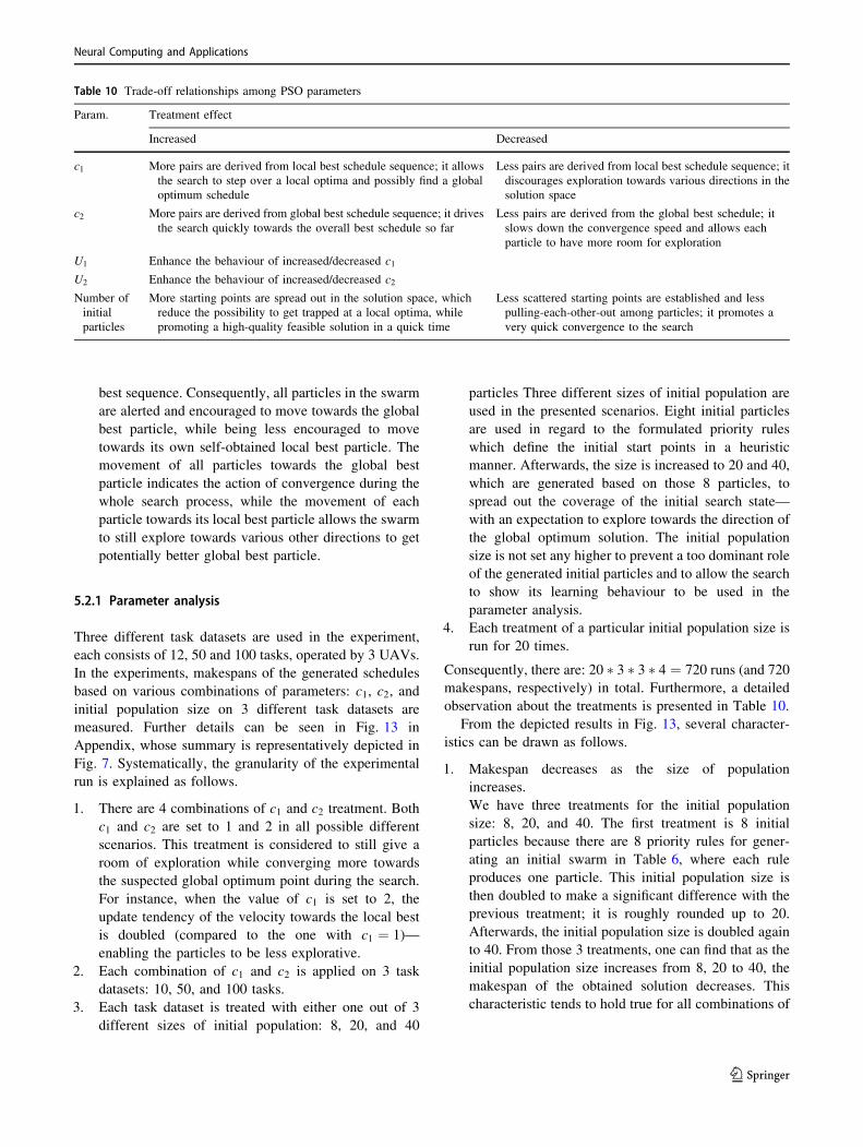
1. There are 4 combinations of c1 and c2 treatment. Both

c1 and c2 are set to 1 and 2 in all possible different

scenarios. This treatment is considered to still give a

room of exploration while converging more towards

the suspected global optimum point during the search.

For instance, when the value of c1 is set to 2, the

update tendency of the velocity towards the local best

is doubled (compared to the one with c1 ¼ 1)—

enabling the particles to be less explorative.

2. Each combination of c1 and c2 is applied on 3 task

datasets: 10, 50, and 100 tasks.

3. Each task dataset is treated with either one out of 3

different sizes of initial population: 8, 20, and 40

particles Three different sizes of initial population are

used in the presented scenarios. Eight initial particles

are used in regard to the formulated priority rules

which define the initial start points in a heuristic

manner. Afterwards, the size is increased to 20 and 40,

which are generated based on those 8 particles, to

spread out the coverage of the initial search state—

with an expectation to explore towards the direction of

the global optimum solution. The initial population

size is not set any higher to prevent a too dominant role

of the generated initial particles and to allow the search

to show its learning behaviour to be used in the

parameter analysis.

4. Each treatment of a particular initial population size is

run for 20 times.

Consequently, there are: 20 � 3 � 3 � 4 ¼ 720 runs (and 720

makespans, respectively) in total. Furthermore, a detailed

observation about the treatments is presented in Table 10.

From the depicted results in Fig. 13, several character-

istics can be drawn as follows.

1. Makespan decreases as the size of population

increases.

We have three treatments for the initial population

size: 8, 20, and 40. The first treatment is 8 initial

particles because there are 8 priority rules for gener-

ating an initial swarm in Table 6, where each rule

produces one particle. This initial population size is

then doubled to make a significant difference with the

previous treatment; it is roughly rounded up to 20.

Afterwards, the initial population size is doubled again

to 40. From those 3 treatments, one can find that as the

initial population size increases from 8, 20 to 40, the

makespan of the obtained solution decreases. This

characteristic tends to hold true for all combinations of

Table 10 Trade-off relationships among PSO parameters

Param. Treatment effect

Increased Decreased

c1 More pairs are derived from local best schedule sequence; it allows

the search to step over a local optima and possibly find a global

optimum schedule

Less pairs are derived from local best schedule sequence; it

discourages exploration towards various directions in the

solution space

c2 More pairs are derived from global best schedule sequence; it drives

the search quickly towards the overall best schedule so far

Less pairs are derived from the global best schedule; it

slows down the convergence speed and allows each

particle to have more room for exploration

U1 Enhance the behaviour of increased/decreased c1

U2 Enhance the behaviour of increased/decreased c2

Number of

initial

particles

More starting points are spread out in the solution space, which

reduce the possibility to get trapped at a local optima, while

promoting a high-quality feasible solution in a quick time

Less scattered starting points are established and less

pulling-each-other-out among particles; it promotes a

very quick convergence to the search

Neural Computing and Applications

123

parameters 1� c1 � 2 and 1� c2 � 2. It is deduced that

the best suited number of initial particles is 40.

2. Makespan leans towards the lowest level as parameter

c2 is set to be greater than c1 Figure 7 depicts the

overall (representing results from 8, 20, and 40 initial

particles) makespans from four combinations of c1 and

c2 values. Each overall makespan is obtained through

applying a local polynomial regression fitting [11]

(with span ¼ 0:75; degree ¼ 2) on the makespan data

from 60 runs, which consists of equal running portions

of experiment with 8, 20, and 40 initial particles (20

runs each). Makespan line of c1 ¼ 1, c2 ¼ 2 is shown

to be lower than others most of the time. This condition

is explained by Eq. (15) where c1 is correlated with the

determination level of the particle to learn from its

local best particle, while c2 is correlated with the

determination level of the particle to learn from the

global best particle.

In this manner, during the iterations of the search,

every particle has the determination to learn more from

a particle which is recalled as the best one by all

particles in the swarm.

5 10 15 20

n − th run

Mak

espa

n

00530002

0091

5 10 15 20

1700

017

500

1800

018

500

1900

019

500

n − th run

Mak

espa

n

5 10 15 20

2900

030

000

3100

032

000

n − th run

Mak

espa

n

(a) (b)

(c)

Fig. 8 Comparison of makespans from the best suited parameters against others. a Number of tasks ¼ 10, b number of tasks ¼ 50, c number of

tasks ¼ 100

Neural Computing and Applications

123

3. Makespan tends to converge at the same convergence

point when the size of the problem is small

Makespan acts as fitness value of a solution. In

Fig. 13a, d, g, j, it is shown that among multiple

distinct runs, a relatively common makespan is found.

That means those different runs have a relatively

common convergence point (of solution). It is an

extreme phenomenon upon the benefit of having highly

spread initial particles in the beginning of the search.

Moreover, since the number of possible solutions is

relatively not high, nearly all local optimum points are

visited, leading to a high chance of finding a global

optimum solution which is the same for all runs.

Consequently, the trade-off relationships among PSO

parameters are depicted in Table 10.

5.2.2 Performance evaluation

Previously, in Fig. 13, the optimality level evaluation for

several sets of parameters has been addressed. Afterwards,

convergence speed evaluation of each set of parameter is

shown, respectively, in Fig. 14. This convergence evalua-

tion is done by checking the value of makespan from the

obtained solution. Once there is no improvement after 10

contiguous iterations, the search is concluded to be con-

verged at that particular iteration. For all combinations,

most of the test cases converged before iteration 40. For the

best case of interest so far, where c1 ¼ 1, c2 ¼ 2, and the

number of initial particles equals to 40, the search managed

to converge under iteration 25. The ultimate goal is to cut

the excessive number of iterations if the search is proven to

most likely converge only after less than the originally

given one. Hence, one might think about cutting the

number of iterations to 30 because even with this limita-

tion, the search is able to bring a good feasible schedule for

the given dataset. However, for a marginal tolerance, the

maximum number of iterations may still be set to 40, the

highest number of iterations so far from all searches. In this

manner, it still gives some space for the search to explore

more if it is trapped in some local optimum points in the

beginning of the search.

6 Results and discussion

From the numerical experiment, the best suited set of

parameters for the search is selected: c1 ¼ 1, c2 ¼ 2,

number of initial particles ¼ 40. In addition, based on a

numerous experiments, the maximum number of itera-

tions ¼ 40 provides a good room for the search to pro-

gress, while higher values are often not worth the increased

computation time. The result is shown in Fig. 8; the graphs

are distinguished by the number of tasks. Each graph rep-

resents points and line (with local polynomial regression

fitting) plot of makespans obtained from search which uses

the best suited set of parameters (represented by triangle

points and full line) against others (represented by circle

points and dashed line), with composition of 20:220,

respectively, resulting in total of 240 makespans plotted in

each graph. The way the data plotted on y-axis is based on

the respective makespan values. As for x-axis, it is based

on the run index values; as mentioned in 5, each set of

parameters is run for 20 times.

In reference with the data shown in Fig. 13, a numerical

summary of the experiments with the best suited parame-

ters on three task datasets is depicted in Table 11. The

presented numbers are in accordance with the makespans

obtained from the best suited parameters, which are dis-

played in Fig. 8. Both (lines in) Fig. 8 and Table 11 can

show a relatively small variance of makespans, which

indicates a stable performance of the best suited

parameters.

Table 11 Numerical summary

of experiments with the best

suited parameters

Parameter Number of tasks Makespan (ms)

c1 c2 Number of initial particles Min Max Average Median

1 2 40 10 1818 1937 1835.85 1818

50 17076 18948 18559.65 18677.5

100 30009 31876 30865.65 30865

10 50 100

050

010

0015

0020

00

Number of tasks

runt

ime

(mill

isec

ond)

averagemedian

Fig. 9 Computation time of the proposed algorithm for the best suited

parameters

Neural Computing and Applications

123

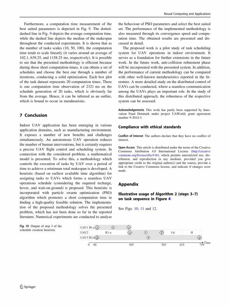
Furthermore, a computation time measurement of the

best suited parameters is depicted in Fig. 9. The dotted-

dashed line in Fig. 9 depicts the average computation time,

while the dashed line depicts the median of the makespan

throughout the conducted experiments. It is shown that as

the number of tasks scales (10, 50, 100), the computation

time tends to scale linearly (it varies around an average of

102.1, 639.25, and 1158.25 ms, respectively). It is possible

to see that the presented methodology is efficient because

during those short computation times, it can obtain a set of

schedules and choose the best one through a number of

iterations, conducting a solid optimization. Each box plot

of the task dataset represents 20 computation times. There

is one computation time observation of 2321 ms on the

schedule generation of 20 tasks, which is obviously far

from the average. Hence, it can be inferred as an outlier,

which is bound to occur in metaheuristic.

7 Conclusion

Indoor UAV application has been emerging in various

application domains, such as manufacturing environment.

It exposes a number of new benefits and challenges

simultaneously. An autonomous UAV operation reduces

the number of human interventions, but it certainly requires

a precise UAV flight control and scheduling system. In

connection with the considered problem, a mathematical

model is presented. To solve this, a methodology which

controls the execution of tasks by UAV over a period of

time to achieve a minimum total makespan is developed. A

heuristic (based on earliest available time algorithm) for

assigning tasks to UAVs which forms a seamless UAV

operations schedule (considering the required recharge,

hover, and wait-on-ground) is proposed. This heuristic is

incorporated with particle swarm optimization (PSO)

algorithm which promotes a short computation time in

finding a high-quality feasible solution. The implementa-

tion of the proposed methodology solves the presented

problem, which has not been done so far in the reported

literature. Numerical experiments are conducted to analyse

the behaviour of PSO parameters and select the best suited

set. The performance of the implemented methodology is

also measured through its convergence speed and compu-

tation time. The obtained results are presented and dis-

cussed in detail.

The proposed work is a pilot study of task scheduling

system for UAV operations in indoor environment. It

serves as a foundation for further extensions in the future

work. In the future work, anti-collision refinement phase

will be incorporated with the presented system. In addition,

the performance of current methodology can be compared

with other well-known metaheuristics reported in the lit-

erature. A more detailed study on the distributed control of

UAVs can be conducted, where a seamless communication

among the UAVs plays an important role. In the study of

this distributed approach, the robustness of the respective

system can be assessed.

Acknowledgements This work has partly been supported by Inno-

vation Fund Denmark under project UAWorld; grant agreement

number 9-2014-3.

Compliance with ethical standards

Conflict of Interest The authors declare that they have no conflict of

interest.

Open Access This article is distributed under the terms of the Creative

Commons Attribution 4.0 International License (http://creative

commons.org/licenses/by/4.0/), which permits unrestricted use, dis-

tribution, and reproduction in any medium, provided you give

appropriate credit to the original author(s) and the source, provide a

link to the Creative Commons license, and indicate if changes were

made.

Appendix

Illustrative usage of Algorithm 2 (steps 3–7)on task sequence in Figure 4

See Figs. 10, 11 and 12.

40 759

R2-d

UAV1UAV2UAV3 d a

R1-e f-d HR1-c

5030 Time625305

cce f

Fig. 10 Output of step 3 of the

schedule creation heuristic

Neural Computing and Applications

123

Step Description3 Task 1

(a) Task availability checkTask 1 is available from time 0.

(b) UAV availability checkUAV1 : 305+228+243+60 = 836UAV2 : 0+260+243+60 = 563UAV3 : 759+346+243+60 = 1408>1200UAV3 needs a recharge.

(c) Overall availability checkUAV1 : 305+228 = 533UAV2 : 0+260 = 260UAV3 : 759+40+2700+260 = 3759

: 759+160+2700+60 = 3679∴ UAV2 is selected for task 1

UAV1

UAV2

UAV3

H

e

f-d

a-ca

b

d d

c c

503 625 759 890 1000 1083 1125

c-e

f

305

Step Description4 Task 4

(a) Task availability checkTask 4 is available from time:

·503 based on task precedence·503 based on position availability

(b) UAV availability checkUAV1 : 533 (305+228)>503+550+60 = 1143UAV2 : 626 (503+123)>503+550+60 = 1236>1200UAV3 : 759 (503+123)>503+346+550+60 = 1715>1200UAV2 and UAV3 need a recharge

(c) Overall availability checkUAV1 : 305+228 = 533UAV2 : 503+260+2700+260 = 3723

: 503+60+2700+60 = 3323UAV3 : 759+40+2700+260 = 3759

: 759+160+2700+60 = 3679∴ UAV1 is selected for task 4.

5 Task 6(a) Task availability checkTask 6 is available from time:

·305 based on task precedence·759 based on position availability

(b) UAV availability checkUAV1 : 1083+241+241+40 = 1605>1200UAV2 : 759 (503+122)<759+241+40 = 1040UAV3 : 759+222+241+40 = 1262>1200UAV1 and UAV3 need a recharge

(c) Overall availability checkUAV1 : 1083+60+2700+160 = 4003

: 1083+160+2700+40 = 3983UAV2 : 759UAV3 : 759+40+2700+160 = 3659

: 759+160+2700+40 = 3659∴ UAV2 is selected for task 6.

6 Task 5(a) Task availability checkTask 5 is available from time:

·305 based on task precedence·305 based on position availability

(b) UAV availability checkUAV1 : 1083+120+235+60 = 1498>1200UAV2 : 1000+127+235+60 = 1422>1200UAV3 : 759+131+235+60 = 1185UAV1 and UAV2 need a recharge

(c) Overall availability checkUAV1 : 1083+60+2700+60 = 3903

: 1083+160+2700+60 = 4003UAV2 : 1000+160+2700+60 = 3920

: 1000+40+2700+60 = 3800UAV3 : 759+131 = 890∴ UAV3 is selected for task 5.

Fig. 11 Output of steps 4–6 of

the schedule creation heuristic

Neural Computing and Applications

123

Makespans of the generated schedules basedon various combinations of parameter values—including c1, c2, and number of initial particles—on task datasets which contain 10, 50, and 100tasks

Each graph in Fig. 13, for instance Fig. 13a, presents the

result of 60 experimental runs. For every set of initial

particles: 8, 20, and 40, the corresponding 20 makespans

are represented as a box plot. This box plot provides a

quick way to examine the distribution of the values, which

is mainly depicted through its quartiles (Q1, median—Q2,

Q3). While the box plot provides a more detailed infor-

mation, an overlaid dotted-dashed line which depicts the

mean of the numerical group gives a more general view of

the data.

UAV1

UAV2

UAV3

R

5 a

1083 3843 4361

b-R1 R1-a

38831143

Step Description7 Task 7

(a) Task availability checkTask 7 is available from time:

·1083 based on task precedence·1083 based on position availability

(b) UAV availability checkUAV1 : 1083+108+478+60 = 1729>1200UAV2 : 1000+222+478+60 = 1760>1200UAV3 : 1125+131+478+60 = 1794>1200UAV1, UAV2, and UAV3 need a recharge

(c) Overall availability checkUAV1 : 1083+ 60+2700+40 = 3883

:1083+160+2700+160 = 4103UAV2 : 1000+160+2700+40 = 3900

: 1000+40+2700+160 = 3900UAV3 : 1125+60+2700+40 = 3925

: 1125+60+2700+160 = 4045∴ UAV1 is selected for task 7.

Fig. 12 Output of step 7 of the

schedule creation heuristic

Neural Computing and Applications

123

8 20 40

size of initial population

mak

espa

n

(a)

size of initial population

mak

espa

n

(b)

size of initial population

mak

espa

n

(c)

size of initial population

mak

espa

n

(d)

size of initial population

mak

espa

n

(e)

size of initial population

mak

espa

n

(f)

size of initial population

mak

espa

n

(g)

size of initial population

mak

espa

n

(h)

size of initial population

mak

espa

n

(i)

size of initial population

mak

espa

n

(j)

size of initial population

mak

espa

n

(k)

8 20 40 8 20 40

8 20 40 8 20 40 8 20 40

8 20 40 8 20 40 8 20 40

8 20 40 8 20 40 8 20 40

2000

2500

3000

3500

1750

018

000

1850

019

000

1950

0

3050

031

000

3150

032

000

1820

1840

1860

1880

1900

1920

1940

1700

017

500

1800

018

500

1900

019

500

3000

030

500

3100

031

500

3200

0

2000

2500

3000

3500

1700

017

500

1800

018

500

1900

019

500

2950

030

000

3050

031

000

3150

032

000

2000

2500

3000

3500

1700

017

500

1800

018

500

1900

019

500

2900

030

000

3100

032

000

size of initial population

mak

espa

n

(l)

Fig. 13 Learning coefficients (c1 and c2) analysis. a c1 ¼ 1, c2 ¼ 1,

number of tasks ¼ 10; b c1 ¼ 1, c2 ¼ 1, number of tasks ¼ 50; cc1 ¼ 1, c2 ¼ 1, number of tasks ¼ 100; d c1 ¼ 1, c2 ¼ 2, number of

tasks ¼ 10; e c1 ¼ 1, c2 ¼ 2, number of tasks ¼ 50; f c1 ¼ 1, c2 ¼ 2,

number of tasks ¼ 100; g c1 ¼ 2, c2 ¼ 1, number of tasks ¼ 10; h

c1 ¼ 2, c2 ¼ 1, number of tasks ¼ 50; i c1 ¼ 2, c2 ¼ 1, number of

tasks ¼ 100; j c1 ¼ 2, c2 ¼ 2, number of tasks ¼ 10; k c1 ¼ 2,

c2 ¼ 2, number of tasks ¼ 50; l c1 ¼ 2, c2 ¼ 2, number of

tasks ¼ 100

Neural Computing and Applications

123

Convergence speed of the search with variouscombinations of parameter values—including c1,c2, and number of initial particles—on taskdatasets which contain 10, 50, and 100 tasks

Each graph in Fig. 14, for instance Fig. 14a, presents the

result of 60 experimental runs. For every set of initial

particles: 8, 20 and 40, the corresponding 20 convergence

speeds are represented as a box plot. This box plot provides

a quick way to examine the distribution of the values,

which is mainly depicted through its quartiles (Q1, med-

ian—Q2, Q3). While the box plot provides a more detailed

information, an overlayed dotted-dashed line which depicts

the mean of the numerical group gives a more general view

of the data.

Neural Computing and Applications

123

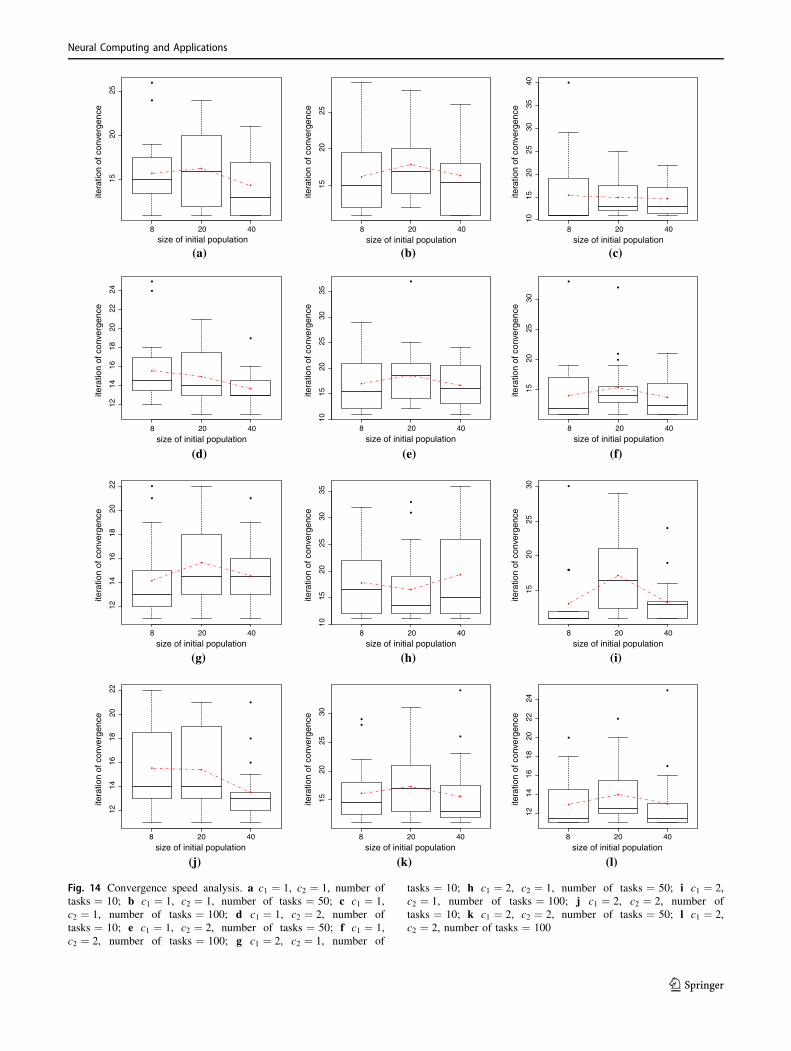
8 20 40

1520

25

size of initial population

itera

tion

of c

onve

rgen

ce

(a)

8 20 40

1520

25

size of initial population

itera

tion

of c

onve

rgen

ce

(b)

8 20 40

1015

2025

3035

40

size of initial population

itera

tion

of c

onve

rgen

ce

(c)

1214

1618

2022

24

itera

tion

of c

onve

rgen

ce

(d)

1015

2025

3035

itera

tion

of c

onve

rgen

ce

(e)

8 20 40

1520

2530

size of initial population8 20 40

size of initial population8 20 40

size of initial population

itera

tion

of c

onve

rgen

ce

(f)

8 20 40

1214

1618

2022

size of initial population

itera

tion

of c

onve

rgen

ce

(g)

8 20 40

1015

2025

3035

size of initial population

itera

tion

of c

onve

rgen

ce

(h)

8 20 40

1520

2530

size of initial population

itera

tion

of c

onve

rgen

ce

(i)

8 20 40

1214

1618

2022

size of initial population

itera

tion

of c

onve

rgen

ce

(j)

8 20 40

1520

2530

size of initial population

itera

tion

of c

onve

rgen

ce

(k)

8 20 40

1214

1618

2022

24

size of initial population

itera

tion

of c

onve

rgen

ce

(l)

Fig. 14 Convergence speed analysis. a c1 ¼ 1, c2 ¼ 1, number of

tasks ¼ 10; b c1 ¼ 1, c2 ¼ 1, number of tasks ¼ 50; c c1 ¼ 1,

c2 ¼ 1, number of tasks ¼ 100; d c1 ¼ 1, c2 ¼ 2, number of

tasks ¼ 10; e c1 ¼ 1, c2 ¼ 2, number of tasks ¼ 50; f c1 ¼ 1,

c2 ¼ 2, number of tasks ¼ 100; g c1 ¼ 2, c2 ¼ 1, number of

tasks ¼ 10; h c1 ¼ 2, c2 ¼ 1, number of tasks ¼ 50; i c1 ¼ 2,

c2 ¼ 1, number of tasks ¼ 100; j c1 ¼ 2, c2 ¼ 2, number of

tasks ¼ 10; k c1 ¼ 2, c2 ¼ 2, number of tasks ¼ 50; l c1 ¼ 2,

c2 ¼ 2, number of tasks ¼ 100

Neural Computing and Applications

123

References

1. Ahner DK, Buss AH, Ruck J (2006) Assignment scheduling

capability for unmanned aerial vehicles: a discrete event simu-

lation with optimization in the loop approach to solving a

scheduling problem. In: Proceedings of the 38th conference on

winter simulation. Winter Simulation Conference, pp 1349–1356

2. Akturk MS, Yilmaz H (1996) Scheduling of automated guided

vehicles in a decision making hierarchy. Int J Prod Res

34(2):577–591

3. Alidaee B, Wang H, Landram F (2009) A note on integer pro-

gramming formulations of the real-time optimal scheduling and

flight path selection of UAVs. IEEE Trans Control Syst Technol

17(4):839–843

4. Tijani IB, Akmeliawati R, Legowo A, Budiyono A, Abdul

Muthalif AG (2014) Hybrid DE-PEM algorithm for identification

of UAV helicopter. Aircr Eng Aerosp Technol Int J

86(5):385–405

5. Bethke B, Valenti M, How JP (2008) UAV task assignment.

IEEE Robot Autom Mag 15(1):39–44

6. Bła _zewicz J, Domschke W, Pesch E (1996) The job shop

scheduling problem: conventional and new solution techniques.

Eur J Oper Res 93(1):1–33

7. Blondin J (2009) Particle swarm optimization: a tutorial. http://cs.

armstrong.edu/saad/csci8100/pso_tutorial.pdf

8. Boucher P (2015) Domesticating the drone: the demilitarisation

of unmanned aircraft for civil markets. Sci Engineering Ethics

21(6):1393–1412

9. Budiyono A, Lee G, Kim GB, Park J, Kang T, Yoon KJ (2015)

Control system design of a quad-rotor with collision detection.

Aircr Eng Aerosp Technol Int J 87(1):59–66

10. Choi BK, Kang DH (2013) Modeling and simulation of discrete

event systems. Wiley, Hoboken

11. Cleveland WS, Grosse E, Shyu WM (1992) Statistical models. In:

Local regression models. Wadsworth & Brooks/Cole, Chapter 8

12. Edis EB, Oguz C, Ozkarahan I (2013) Parallel machine

scheduling with additional resources: notation, classification,

models and solution methods. Eur J Oper Res 230(3):449–463

13. Fasano G, Accardo D, Moccia A, Carbone C, Ciniglio U, Corraro

F, Luongo S (2008) Multi-sensor-based fully autonomous non-

cooperative collision avoidance system for unmanned air vehi-

cles. J Aerosp Comput Inf Commun 5(10):338–360

14. Garey MR, Johnson DS (1979) A guide to the theory of NP-

completeness. WH Freemann, New York

15. Garey MR, Johnson DS (2002) Computers and intractability, vol

29. WH Freeman, New York

16. Garrido A, Salido MA, Barber F, Lopez M (2000) Heuristic

methods for solving job-shop scheduling problems. In: Proceed-

ings of the ECAI-2000 workshop on new results in planning,

scheduling and design (PuK2000). pp 44–49

17. Gunter CA, Gunter EL, Jackson M, Zave P (2000) A reference

model for requirements and specifications. In: Proceedings of the

4th international conference on requirements engineering. IEEE,

pp 189

18. Hassan R, Cohanim B, De Weck O (2005) Venter Gerhard A

comparison of particle swarm optimization and the genetic

algorithm. In: Proceedings of the 1st AIAA multidisciplinary

design optimization specialist conference. pp 1–13

19. Hou Z-L, Guo X-P (2013) Parallel machine scheduling with

resources constraint and sequence dependent setup times. In:

Proceedings of 2012 3rd International Asia Conference on

Industrial Engineering and Management Innovation (IEMI2012).

Springer, pp 801–811

20. Kellerer H, Strusevich VA (2008) Scheduling parallel dedicated

machines with the speeding-up resource. Nav Res Logist

55(5):377–389

21. Kennedy J (2010) Particle swarm optimization. In: Encyclopedia

of machine learning. Springer, pp 760–766

22. Khosiawan Y, Nielsen I (2016) A system of UAV application in

indoor environment. Prod Manuf Res 4(1):2–22

23. Khosiawan Y, Nielsen I, Do NAD, Yahya BN (2016) Concept of

indoor 3d-route UAV scheduling system. In: Information systems

architecture and technology: proceedings of 36th international

conference on information systems architecture and technology—

ISAT 2015—part I. Springer, pp 29–40

24. Jonghoe Kim, Morrison James R (2014) On the concerted design

and scheduling of multiple resources for persistent UAV opera-

tions. J Intell Robot Syst 74(1–2):479–498

25. Kim J, Song BD, Morrison JR (2013) On the scheduling of

systems of UAVs and fuel service stations for long-term mission

fulfillment. J Intell Robot Syst 70(1–4):347–359

26. Kim Y, Gu D-W, Postlethwaite I (2007) Real-time optimal

mission scheduling and flight path selection. IEEE Trans Auto-

mat Control 52(6):1119–1123

27. Liu Z (2007) Investigation of particle swarm optimization for job

shop scheduling problem. In: Third International Conference on

Natural Computation, ICNC 2007, volume 3. IEEE, pp 799–803

28. Iwan Mahmud, Rini Akmeliawati, Agus Budiyono (2014) DE-

based robust controller design for helicopter cruise control. Int J

Robot Mechatron 1(4):145–151

29. Mitchell JE (2002) Branch-and-cut algorithms for combinatorial

optimization problems. Handb Appl Optim 2:65–77

30. Nigam N, Bieniawski S, Kroo I, Vian J (2012) Control of mul-

tiple UAVs for persistent surveillance: algorithm and flight test

results. IEEE Trans Control Syst Technol 20(5):1236–1251

31. Nilakantan JM, Ponnambalam SG, Jawahar N, Kanagaraj G

(2015) Bio-inspired search algorithms to solve robotic assembly

line balancing problems. Neural Comput Appl 26(6):1379–1393

32. Park Y, Khosiawan Y, Moon I, Janardhanan MN, Nielsen I

(2016) Scheduling system for multiple unmanned aerial vehicles

in indoor environments using the CSP approach. In: Intelligent

decision technologies 2016. Springer, pp 77–87

33. Piciarelli C, Micheloni C, Martinel N, Vernier M, Foresti GL

(2013) Outdoor environment monitoring with unmanned aerial

vehicles. In: International Conference on Image Analysis and

Processing—ICIAP 2013. Springer, pp 279–287

34. Ponnambalam SG, Aravindan P, Naidu GM (2000) A multi-ob-

jective genetic algorithm for solving assembly line balancing

problem. Int J Adv Manuf Technol 16(5):341–352

35. Qi X, Chen T, Tu F (1999) Scheduling the maintenance on a

single machine. J Oper Res Soc 50(10):1071–1078

36. Rameshkumar K, Suresh RK, Mohanasundaram KM (2005)

Discrete particle swarm optimization (DPSO) algorithm for per-

mutation flowshop scheduling to minimize makespan. In: Inter-

national conference on natural computation. Springer,

pp 572–581

37. Rothkopf MH (1966) Scheduling independent tasks on parallel

processors. Manag Sci 12(5):437–447

38. Semiz F (2015) Task assignment and scheduling in UAV mission

planning with multiple constraints. Ph.D. Thesis, Middle East

Technical University

39. Sha DY, Hsu C-Y (2006) A hybrid particle swarm optimization

for job shop scheduling problem. Comput Ind Eng 51(4):791–808

40. Sha DY, Lin H-H (2010) A multi-objective pso for job-shop

scheduling problems. Expert Syst Appl 37(2):1065–1070

41. Shaw P (2004) A constraint for bin packing. In: International

conference on principles and practice of constraint programming.

pp 648–662

Neural Computing and Applications

123

42. Shima T, Rasmussen SJ, Sparks AG (2005) UAV cooperative

multiple task assignments using genetic algorithms. In: American

Control Conference, 2005. Proceedings of the 2005. IEEE,

pp 2989–2994

43. Shima T, Schumacher C (2005) Assignment of cooperating

UAVs to simultaneous tasks using genetic algorithms. Defense

Technical Information Center, San Francisco, California

44. Sorensen K, Glover FW (2013) Metaheuristics. In: Encyclopedia

of operations research and management science. Springer,

pp 960–970

45. Tijani IB, Akmeliawati R, Legowo A, Budiyono A (2014)

Nonlinear identification of a small scale unmanned helicopter

using optimized NARX network with multiobjective differential

evolution. Eng Appl Artif Intell 33:99–115

46. Valenti M, Dale D, How J, Vian J (2007) Mission health man-

agement for 24/7 persistent surveillance operations. In: AIAA

guidance, control and navigation conference. Myrtle Beach, SC

47. von Bueren SK, Burkart A, Hueni A, Rascher U, Tuohy MP, Yule

IJ (2015) Deploying four optical uav-based sensors over grass-

land: challenges and limitations. Biogeosciences 12(1):163–175

48. Weinstein AL, Schumacher C (2007) UAV scheduling via the

vehicle routing problem with time windows. In: Proceedings of

the AIAA infotech@ aerospace 2007 conference and exhibit.

Rohnert Park, California

49. Xu D, Sun K, Li H (2008) Parallel machine scheduling with

almost periodic maintenance and non-preemptive jobs to mini-

mize makespan. Comput Oper Res 35(4):1344–1349

50. Zeng J, Yang X, Yang L, Shen G (2010) Modeling for UAV

resource scheduling under mission synchronization. J Syst Eng

Electron 21(5):821–826

51. Zobolas GI, Tarantilis CD, Ioannou G (2008) Exact, heuristic and

meta-heuristic algorithms for solving shop scheduling problems.

In: Metaheuristics for scheduling in industrial and manufacturing

applications. Springer, pp 1–40

Neural Computing and Applications

123