Task-Dependent Spatial Sensitivity in Area A1,

DZ, and PAF of Cat Auditory Cortex

by

Chen-Chung Lee

A dissertation submitted in partial fulfillment of the requirements for the degree of

Doctor of Philosophy (Neuroscience)

in The University of Michigan 2010

Doctoral Committee:

Professor John C. Middlebrooks, University of California, Irvine, Co-Chair Research Professor Susan E. Shore, Co-Chair Professor Stephen A. Maren Associate Professor J. Wayne Aldridge Associate Professor Gina R. Poe

ii

Dedicated to My Parents

for their love and support

iii

ACKNOWLEDGEMENTS

This dissertation work would not have been possible without the guidance of my

mentors, support of my friends, and love of my family. I am deeply appreciative for all

the talented people around me that helped educate me to be an open-minded scientist and

mature man after this incredible journey.

I especially want to express my gratitude to my mentor, John Middlebrooks. He

is a wonderful teacher who always guided me into the right direction with encouragement

and support. He is a great scientist full of knowledge and insightful ideas. He is also a

good friend that is always understanding and patient with me. It has been a great honor

to work with him. I thank him for being the charioteer of the progress of this work and at

the same time, allowing me to explore freely in the field and figure things out on my own.

I would also like to thank members of my dissertation committee, Susan Shore, Steve

Maren, Wayne Aldridge, and Gina Poe for their consistent guidance and helpful feedback.

It has been a great pleasure to work in the Middlebrooks’ lab. The unwavering

encouragement and the support from the past and current members of the lab have made

my time as a Ph.D. student into a rewarding life experience. Alana Kirby and Zekiye

Onsan have traveled across the continent from Michigan to California with me. They

made invaluable contributions to my manuscripts and my research. My gratitude for their

unselfish support and sharing was beyond words. We have become a small family with

iv

much of love and care inside and outside of the lab. All those moments that we shared

together is one of the greatest memory I have. I would also like to thank Ewan

Macpherson, who was the best tutor and the best friend and who helped me with a lot of

data analysis and experiments. It is important to note that this work would not have

begun without Ian Harrington and Chris Stecker. All the insightful discussions and the

inspiring ideas had tremendous influences on the development of this project. Also,

many people at the Kresge Hearing Research Institue, especially Jim Wiler, Beth Hand,

Chris Ellinger, Dwayne Vailliencourt and Jackie Black, have assisted me to overcome

many difficulties in research with their expertise and friendship. I would like to

acknowledge the help and support of the expert veterinary staffs in Unit for Laboratory

Animal Medicine. My research relied on the animals’ well-being. Thanks to Gail Rising

at the Animal Surgery Operating Room, Kristie Brock, Christine Alvarado and Karen

Rogers to ULAM for their efforts and dedications for animal health and wellness, which

made my research possible. I also want to thank the Neuroscience Graduate Program, in

particular, Rich Hume, Peter Hitchcock, and Yehoash Raphael, for introducing me into

Neuroscience and providing me an excellent academic environment. I also appreciated

the funding support by the Program In Biomedical Sciences and John Middlebrooks’

RO1 grant from NIDCD over the years.

Finally, I thank my family and friends. I am such a lucky guy to have so many

wonderful and talented people surrounding me. I especially want to thank my parents and

my sister; with their unconditional love and support, I was able to carry on after all the

challenges that I have encountered. I would like to thank all my excellent and lovely

friends who made the world and my life as a graduate student much more interesting, in

v

particular, I thank Hsien-Chang Lin, Yi-Chen Chen, Yin-Ting Yeh, Tsu-Wei Wang,

Jenn-Yah Yu, YuFen Chang, and Kuo-Wei Huang, for their endless encouragement and

great company over the years.

Last but certainly not least, I thank Bucket, Miss Jackson, Karma, Lucky and

Belle for their irreplaceable contributions to my research. I will never forget the time we

spent together.

vi

TABLE OF CONTENTS

DEDICATION…………………………..………………………………….ii

ACKNOWLEDGEMENTS………………………………………………iii

LIST OF FIGURES…………………………………………………….....ix

ABSTRACT…...……………………………….…………...……………..xii

CHAPTER 1. Introduction………………………………………..……………………….….1

1.1 Sound localization and the representation of spatial information in the auditory system…………………………………...……………….......1

1.2 Spatial sensitivity in the auditory cortex……………..………………..5

1.3 Dynamics of spatial hearing……………………………..…………….8

2. Methods………………………………………………………...….………….11

2.1 Stimulus generation…………………………..……………..……….11

2.2 Behavioral tasks and training………………….……..………...…….12

2.3 Surgery…………………………………………….…………............14

2.4 Physiological recording……………………………………………...16

2.5 Data analysis…………………………………………………………17

3. Task-Dependent Dynamics of Spatial Sensitivity in the Primary Auditory Cortex (A1)……...…………………………………………………………..25

3.1 Introduction……….……………………………………….………...25

3.2 Results…………….…………………………………………….…...27

vii

3.2.1 General characteristics of spatial selectivity and temporal firing patterns……...…………………………………….....................27

3.2.2 Quantitative measures of task dependence of responses……....31

3.2.3 The increase in spatial sensitivity comes from suppression of responses to least-favored stimuli………..…………………….37

3.2.4 Time course of task-dependent modulation of spatial tuning……………………………………………..……………38

3.3 Discussion…………………………………………..………………..40

4. Comparison of Spatial Selectivity and Temporal Firing Patterns in A1,

DZ and PAF.………………………….………………..………...………….47

4.1 Introduction………………….………………………….………..…..47

4.2 Results and Discussion………………….…………………………...49

4.2.1 General characteristics of spatial selectivity and temporal firing patterns in DZ……………..………………………………...…49

4.2.2 General characteristics of spatial selectivity and temporal firing patterns in PAF………………..……………………………….52

4.2.3 Quantitative measures of spatial sensitivity: comparison across A1, DZ and PAF………………………………..……………...58

4.2.4 Comparison of first spike latency between awake and anesthetized conditions…………………………………….…..65

4.3 Summary…………………………………………………..…………67

5. Task-Dependent Modulation of Spatial Sensitivity in A1, DZ and PAF....69

5.1 Introduction……………………………..……………………………69

5.2 Results and Discussion…………………………….………………...70

5.2.1 Quantitative measures of task dependence of responses across three cortical fields: best area……………………………….....73

5.2.2 Quantitative measures of task dependence of responses across three cortical fields: onset activity…………………………..…77

5.2.3 Quantitative measures of task dependence of tonic activity…...82

5.2.4 Task-dependent modulation of first spike latencies……………84

5.3 Summary………………..……………………………………………85

viii

6. Location Coding by Individual Units and Ensembles…………………..…88

6.1 Introduction………………………………………………………..…88

6.2 Results and Discussion……………………………………………....89

6.2.1 The transmitted spatial information of individual units………..89

6.2.2 The transmitted spatial information of an ensemble of units randomly chosen from whole population of A1, DZ and PAF…………………………………………………………….90

6.2.3 The transmitted spatial information of ensemble of units with higher spatial sensitivity: DZ and PAF………………………...93

6.3 Summary……………………………………………………………..97

7. General Discussion…………..……………………………………………….99

7.1 Awake A1, DZ and PAF showed more distinct differences compared to anesthetized studies………………………………..……………..100

7.2 A1 showed stronger task-dependent modulation of spatial sensitivity compared to DZ and PAF……………………………….………….103

7.3 PAF units showed more distributed best areas and better location coding…………………………………………………..…………...106

7.4 Is DZ the area responsible for capturing the stimulus from the center and excluding stimuli from the side?.................................................108

BIBLIOGRAPHY.....................................................................................111

ix

LIST OF FIGURES

Figure

1.1 Lateral view of the left hemisphere of cat cerebral cortex showing the positions of the different auditory cortical areas………………………………6

2.1 Spike raster, correspondent PSTH and computation of ERRF width of an example A1 unit…...…………………………………………………………21

3.1 Task-dependant modulation of spatial sensitivity……..……………………..28

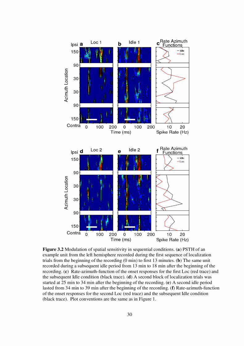
3.2 Modulation of spatial sensitivity in sequential conditions……..…………….30

3.3 PSTH plots in three task conditions from two units that showed offset dominant responses…………………………………………..………………32

3.4 Comparisons of ERRF widths across condition-pairs for all units with excitatory responses within first 40ms after stimulus onset………………....34

3.5 Percentage of units that showed significant sharpening or broadening of spatial tuning between condition pairs…………………………………….....35

3.6 First spike latency for favored locations was longer and more dispersed during behavioral conditions…………………………………………………….…..36

3.7 Spike rates decreased in the localization condition primarily for stimuli at non-favored locations………………………………………………………...38

3.8 Time course of the task-dependent modulation of the response at the least-favored locations……………………………………………………………..40

4.1 DZ units showed strong preference for stimuli near frontal midline………...51

4.2 PAF units showed best areas evenly distributed across space…………….....53

4.3 Inhibitory responses in PAF…………………………………….....................55

4.4 Complex inhibitory responses in PAF sometimes were accompanied by

complementary excitatory responses from other units nearby……………....56

4.5 Onset dominant units in PAF………………………………………………...57

x

4.6 Comparison of best areas across three cortical fields………………………..59

4.7 Accumulated distributions of ERRF widths ………………………………...60

4.8 Comparison of best areas v.s. ERRF width across three cortical fields…......61

4.9 Best areas for tonic units in DZ and PAF…………………………………....63

4.10 Onset v.s. Tonic ERRF widths for tonic units in DZ and PAF……………..64

4.11 First spike latencies in A1, DZ and PAF…………………………………...67

5.1 Three example DZ units in Idle, Timbre Discrimination and Localization conditions………………………………………………………………….…72

5.2 Three example PAF units with azimuth-dependent tonic responses in Idle,

Timbre Discrimination and Localization conditions………………………...74

5.3 Comparison of best areas in Idle versus Localization conditions across three

cortical areas…………………………………………………………….…...76

5.4 Ipsi-Contra Ratio was higher during behavioral tasks for CI units…….……77

5.5 Onset ERRF widths across behavioral conditions in A1, DZ and PAF…..….78

5.6 Percentage of units that showed significant sharpening or broadening of

spatial tuning between behavioral conditions pairs in A1, DZ and PAF….....80

5.7 The sharpening of spatial tuning resulted from suppression of spike rates for

least-favored locations……………………………………………………….81

5.8 Best areas of tonic responses in DZ and PAF between Idle versus Localization conditions …………………………………………………………………....82

5.9 Onset and tonic ERRF widths for tonic units in DZ and PAF…………….....83

5.10 The spike rates of the tonic responses for the favored stimuli increased during the Localization conditions compared to Idle conditions…………….84

5.11 Behavioral modulation of first spike latency in A1, DZ and PAF……….....86

6.1 Transmitted information of individual units across population in A1, DZ and

PAF…………………………………………………………………………..90

6.2 Transmitted information of ensembles across population in A1, DZ and

PAF units.........................................................................................................92

xi

6.3 Transmitted information of ensembles selected from the sharply-tuned

midline units in DZ…………………………………………………………..94

6.4 Transmitted information of ensembles selected from the sharply-tuned

midline units in DZ……………………………………………….………….96

xii

ABSTRACT

Auditory cortex is essential for normal sound localization behavior. Earlier studies

showed that ablations of auditory cortex produced behavioral deficits in sound

localization. More recently, reversible inactivation of auditory cortical primary auditory

area (A1), dorsal zone (DZ) or posterior auditory field (PAF) in cats has demonstrated

varying degrees of localization deficits, from moderate (A1 & DZ) to severe (PAF).

Physiological studies from our lab in anesthetized animals have demonstrated that the

representation of any particular sound-source location is highly distributed among and

within cortical fields. Nevertheless, those studies in anesthetized conditions demonstrate

marked differences in spatial sensitivity among areas A1, DZ, and PAF. The overall goal

of the current study was to characterize the auditory spatial sensitivity of neurons in A1,

DZ and PAF in awake animals and to test the influence of an animal’s attentional state on

the representation of sound-source location by firing patterns of cortical neurons.

We recorded extracellular spike activity from cats’ auditory cortex with chronically

implanted 16-channel probes. In all conditions, the spatial receptive field of each neuron

was assessed by 80 ms broadband noise-burst probe stimuli played from free field

speakers in the horizontal plane, spaced in 20 degree increments. We compared the

behavioral task dependence of spatial sensitivity in these three conditions: 1) Idle --

exposed to probe stimuli without engaging in behavior tasks; 2) Timbre Discrimination --

xiii

detecting a change from the probe stimulus to a click train, regardless of the location of

the sound; and 3) Localization -- distinguishing a shift in stimulus elevation to 40 or more

degrees above horizontal plane. All three conditions were compared within single ~1.5-hr

sessions.

Overall, we found that neurons in area A1 tended to have broad spatial tuning, with

spatial receptive fields ranging from hemifield to omnidirectional. In area DZ, neurons

tended to respond best to stimuli near the frontal midsagittal plane. In area PAF, neurons

with sharp spatial tuning exhibited best areas more evenly distributed across space.

Neurons in A1 exhibited stronger task dependent modulation of their responses than did

neurons in DZ and PAF. During the localization task, many A1 neurons reduced their

spatial receptive fields from omnidirectional to hemifield by suppressing their responses

to least-favored stimuli. Spatial sharpening occurred on a scale of tens of seconds and

could be replicated multiple times within single ~1.5-hr test sessions. That and an

observed increase in latencies suggest an important role of inhibitory mechanisms. In

areas DZ and PAF, the behavioral conditions usually were associated with an increase of

tonic firing to the favored stimuli in addition to the suppression of responses to the least-

favored stimuli. The location-related information conveyed by the temporal firing

patterns among a small ensemble of DZ and PAF units was higher during the behavioral

conditions than in the Idle condition. The differential task-dependent modulation of

spatial sensitivity among these three areas, as well as the differences in distribution of

spatial receptive fields, suggests that these three cortical areas might play distinct roles in

auditory spatial processing.

1

CHAPTER 1

Introduction

1.1 Sound localization and the representation of spatial information in

the auditory system

Sound localization is essential for animal survival and is also crucial for our daily

life. The ability to localize a sound source is necessary for an animal to locate prey or

avoid a predator. For human listeners in particular, the ability to localize and segregate

sound sources in a complex auditory environment improves speech intelligibility and the

identification of sounds of interest. However, unlike the visual or somatosensory systems,

spatial information is not organized in a topographical way within the peripheral auditory

system. Listeners localize a sound by using the acoustic cues created by interaural

differences or the direction-dependent filter created by the shape of pinna and the size of

the head. For a sound originating in a location with a lateral azimuth, the sound wave

arrives at one ear earlier than the other ear, generating an interaural time difference (ITD)

cue. ITD cues are more important for low frequency sound, since the phase delays are

more prominent for low frequency sound. Another cue is generated when sounds off the

2

midline reach the closer ear at a higher sound level than the farther ear, which receives

sound waves attenuated by the shadowing effect of the head. This cue, interaural level

difference (ILD), is the dominant cue for localizing high frequency sound since the

attenuation is greater for high frequencies. Neither ITD nor ILD cues provide

information about the vertical location of a sound source. Monaural spectral cues created

by the head-related transfer function (HTRF) are required to accurately localize sounds in

the vertical dimension. Therefore, the auditory system needs to integrate the interaural

and the monaural cues in order to successfully locate a sound source in three dimensions.

Sound arrives at the cochlea after travelling through external and middle ear. In the

cochlea the acoustic information is transduced into neural signals by the hair cells then

sent to the cochlear nucleus (CN) via auditory nerves. The cochlear nucleus is the first

site of the neuronal processing for the acoustic information for sound localization.

Previous studies have suggested that the neurons in dorsal cochlear nucleus might be

sensitive to the change of the spectral edge of the stimulus (Nelken and Young, 1996;

Reiss and Young, 2005) , which is an important cue for vertical sound localization in cats

(Huang and May, 1996; May, 2000) . Although traditionally the CN was considered as a

monaural nucleus which received major input from ipsilateral cochlea, recent studies

have suggested that the direct or indirect contralateral input might also modulate the

responses in CN (Ingham et al., 2006; Shore et al., 1992; Sumner et al., 2005). In

addition, the dorsal cochlear nucleus also receives somatosensory inputs from spinal

trigeminal nuclei (Itoh et al., 1987; Shore, 2005; Shore and Zhou, 2006). This multi-

sensory integration between somatosensory and auditory systems in CN has been

3

suggested to play important role in adaptation for the effects of pinna orientation on

sound-localization cues (Kanold and Young, 2001).

Ipsilateral and contralateral CN both project to the medial superior olivary nucleus

(MSO), where clear evidence of binaural information convergence can be found. Units in

MSO tend to be excitatory-excitatory (E-E type) in that the summation of inputs from

both sides causes an increase in firing rate. Since the neural signals from the contralateral

side travel a longer distance than the ipsilateral signals, MSO units are thought to be

specialized for ITD information due to this coincidence detection system. The lateral

superior olivary nucleus (LSO) is also thought to play an important role for sound

localization. LSO receives excitatory input from ipsilateral cochlear nucleus and

inhibitory input from contralateral cochlear nucleus indirectly through MNTB. Thus, the

excitatory-inhibitory (E-I) nature of LSO units was thought to be sensitive to ILD. The

fact that MSO has more low frequency neurons than the LSO and LSO has more high

frequency neurons is also consistent with the sensitivity of ITD information in MSO and

the sensitivity of ILD information in LSO. Both MSO and LSO project to inferior

colliculus (IC) via the lateral lemniscus. The central nucleus of the inferior colliculus

(ICC) is the first station to integrate of all the auditory ascending pathways. In addition

to the inputs from MSO and LSO, it also receives direct inputs from contralateral

cochlear nucleus. Units in ICC have been found to be sensitive to both ITD and ILD cues

(Davis et al., 1999; Loftus et al., 2004; Ramachandran and May, 2002). Furthermore,

earlier studies suggested that there are units in ICC that respond differentially to the

complex spectral cues or spectral notches created by HRTFs, which reflects sensitivity to

changes in the vertical location (Davis et al., 2003). This evidence suggests that the ICC

4

might play an important role in integrating binaural and monaural cues to create a

representation of auditory space. Earlier studies of the ICC itself showed no evidence of a

topographical representation of auditory space, but there was evidence suggestive of such

a map in a nucleus post-synaptic to the ICC: the nucleus of the brachium of the inferior

colliculus (BIN). Previous study has suggested an existence of an auditory map in the

ICX in guinea pigs (Binns et al., 1992). Studies in the barn owl have also found a map of

auditory space in the nucleus homologous to the mammalian ICX (Gutfreund and

Knudsen, 2006; Knudsen and Konishi, 1978).

The main projections from IC are to the ventral and medial divisions of medial

geniculate body (MGB) in the thalamus and the superior colliculus (SC) in the midbrain

via the ICX (Kudo and Niimi, 1980). The MGB is a specific thalamic auditory relay

between colliculus and auditory cortex. A previous study has shown that the spatial

sensitivity of MGB units resembled the units seen in ICC and the ones seen in primary

auditory cortex, in the sense that the spatial receptive fields of MGB units usually showed

strong contralateral tuning or broad omnidirectional sensitivity (Samson et al., 2000).

The SC in general is regarded not primarily as an auditory structure but as a structure that

integrates information among different sensory modalities, including visual, tactile, and

auditory inputs, and motor output. The most important function of SC is probably the

ocular-motor control (e.g. reflexive orienting saccade). Previous studies have found that

units in SC showed relatively sharp spatial tuning and that there is a topographical

organization of the auditory receptive fields, roughly lining up with the visual receptive

fields (King and Hutchings, 1987; Middlebrooks and Knudsen, 1984)

5

So far we have discussed the representation of spatial information in sub-cortical

levels of the auditory pathway. Auditory spatial information seems to be distributed

along the auditory pathway and only the SC contains a more complete representation in

mammalian auditory system. However, the mission for the central nervous system to

solve the problem about where the sound comes from is not completed at the level of the

thalamus, or even the SC. Previous studies have shown that intact auditory cortex was

required for sound localization behavior (Jenkins and Merzenich, 1984; Malhotra et al.,

2004; Wortis and Pfeffer, 1948). In the next section, we will review previous studies

about the spatial representation in the cortex and discuss how those motivated the current

study.

1.2 Spatial sensitivity in the auditory cortex

Previous studies have shown that ablations of auditory cortices produced deficits in

sound localization (Clarke et al., 2000; Heffner, 1997; Heffner and Heffner, 1990;

Jenkins and Merzenich, 1984; Kavanagh and Kelly, 1987; Wortis and Pfeffer, 1948).

Recently, the studies from Lomber and colleagues of 19 cortical fields via reversible

inactivation technique (Malhotra et al., 2004; Malhotra et al., 2008) have provided

insightful evidence of the contribution of auditory cortices to sound localization. They

found that reversible inactivation of auditory cortical areas A1, DZ, PAF produced

deficits in sound localization performance while inactivation of other fields had no effects.

However, the deficits after deactivation differ among the three areas: deactivation of A1

or DZ only produced moderate deficits in localization performance: when deactivating

A1, the performance accuracy reduced from 90% to 43%; the errors were usually closer

6

and in the same hemifield as the targets (errors usually ≤ 30°). When deactivating DZ,

the performance accuracy reduced from 93% to 69%; however, the errors produced after

DZ deactivation tended to be much larger (≥ 60°) and were more likely to be in the

incorrect hemifield. When deactivating PAF alone, it produced severe deficits in

localization performance; the performance accuracy dropped from about 85% correct to

just above chance (7.7 % correct); the errors produced after PAF deactivation were larger

than A1 and usually were in the same hemifield as the targets (errors usually ≤ 60°).

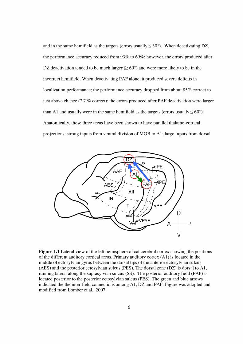
Anatomically, these three areas have been shown to have parallel thalamo-cortical

projections: strong inputs from ventral division of MGB to A1; large inputs from dorsal

Figure 1.1 Lateral view of the left hemisphere of cat cerebral cortex showing the positions of the different auditory cortical areas. Primary auditory cortex (A1) is located in the middle of ectosylvian gyrus between the dorsal tips of the anterior ectosylvian sulcus (AES) and the posterior ectosylvian sulcus (PES). The dorsal zone (DZ) is dorsal to A1, running lateral along the suprasylvian sulcus (SS). The posterior auditory field (PAF) is located posterior to the posterior ectosylvian sulcus (PES). The green and blue arrows indicated the the inter-field connections among A1, DZ and PAF. Figure was adopted and modified from Lomber et al., 2007.

7

and rostral pole nuclei of MGB to DZ; large inputs from dorsal superficial and

ventrolateral nuclei of MGB to PAF (Lee and Winer, 2008a). These three

areas also have strong inter-field cortical connections: PAF receives strong non-

reciprocal inputs from A1(Carrasco and Lomber, 2009; Lee and Winer, 2008b), and DZ

receives strong inputs from both A1 and PAF (Lee and Winer, 2008b). Together, these

findings suggest that the auditory spatial percept may rely on the cortical activities; also,

A1, DZ and PAF might work together as a cortical network for sound localization and

each field might contribute differently in processing spatial information.

A number of electrophysiological studies from our lab and other groups have

studied the spatial sensitivity in different auditory cortical areas in anesthetized cats: [A1:

(Eggermont, 1998; Middlebrooks et al., 1994; Middlebrooks and Pettigrew, 1981; Reale

and Brugge, 2000; Reale et al., 2003), A2: (Furukawa et al., 2000; Middlebrooks et al.,

1998; Xu et al., 1998), AES: (Las et al., 2008; Middlebrooks et al., 1998), PAF: (Stecker

et al., 2003), DZ: (Stecker et al., 2005a; Stecker et al., 2005b) and AAF: (Harrington et

al., 2008)], macaques [A1: (Ahissar et al., 1992; Benson et al., 1981), and CM:

(Recanzone, 2000)] and ferrets [A1: (Bizley et al., 2009; Schnupp et al., 2001)]. These

studies generally found that there were location-sensitive units showing variation in the

spike rates and spike latencies across space within auditory cortices. The majority of

cortical neurons preferred contralateral stimuli. Their spatial receptive fields were

usually broad; most of them responded omnidirectionally to the stimuli or showed more

restricted activities to the contralateral field. Some of the non-primary cortical fields

showed higher spatial sensitivity (e.g. DZ and PAF in cats, Stecker et al., 2003; Stecker et

al., 2005; CM in macaques, Recanzone et al., 2000) than others (e.g. A1 or AAF in cats),

8

but the differences among cortical fields were quantitative than qualitative. Moreover,

none of these studies has identified any cortical field that exhibited a topographical

organization of auditory space.

So far most of those electrophysiological studies of the spatial representation in

the cortex described above were recorded in anesthetized animals. Anesthesia has been

shown to have strong effects on the activities of cortical neurons (Cheung et al., 2001;

Gaese and Ostwald, 2001; Zurita et al., 1994). Our previous study in awake A1 has

shown that, under awake conditions, units showed a variety of response patterns that

were not observed under anesthesia (Mickey and Middlebrooks, 2003). Moreover, units’

spatial tuning was higher and more level-invariant in awake conditions compared to

anesthetized conditions. Our previous studies have suggested that DZ and PAF have

higher spatial sensitivity under anesthetized conditions. Therefore, in the current

research, we further compared the spatial sensitivity in awake DZ and PAF to those in A1.

Overall, we found some qualitative and quantitative differences in the spatial sensitivity

of the cortical neurons among these three areas. We present those results in Chapter 4

and 5.

1.3 Dynamics of spatial hearing

Perception of auditory spatial location is thought to be a primary sensation.

However, this primary sensation can be shaped by experience and modulated by spatial

attention. Plasticity of spatial hearing has been demonstrated in previous psychophysics

studies, which have shown that subject’s sound localization performance improved after

training (Recanzone, 1998; Spierer et al., 2007; Wright and Fitzgerald, 2001). Studies

9

with modified pinnae cues also showed that sound localization can be re-calibrated after

long-term learning (Hofman et al., 1998; Kacelnik et al., 2006; King et al., 2000).

The dynamics of spatial hearing can also be observed from studies of spatial

attention. Previous reports have shown that subjects localized or identified the sounds

more efficiently when they had prior knowledge about the target locations (Arbogast and

Kidd, 2000; Johnen et al., 2001; McDonald and Ward, 1999; Mondor and Zatorre, 1995;

Rhodes, 1987; Roberts et al., 2009; Spence and Driver, 1994). This ability of orienting

auditory attention to certain spatial locations also benefits subjects’ performance in

identifying a specific talker from a multi-talker conversation or focuses on a particular

sound in a noisy environment, like in a cocktail party (Allen et al., 2009; Best et al., 2008;

Ihlefeld and Shinn-Cunningham, 2008; Kidd et al., 2005). The perception of auditory

space can shift away from the adapted location after prolonged exposure to the sounds

from that location (Carlile et al., 2001; Dingle et al., 2010; Kopco et al., 2007) However,

the underlying neural mechanism for how attention modulates the spatial representation

to achieve the behavioral task demands is still poorly understood.

In our previous study of A1 in awake cats (Mickey and Middlebrooks, 2003), we

found that the spatial sensitivity were greater than in anesthetized conditions and that the

spatial tuning and the transmitted information within the temporal response pattern were

level-invariant. In the present study, we found that there was a subset of DZ units that had

sharper spatial tuning with strong preferences for midline stimuli and a subset of PAF

units that were also sharply tuned but with best areas evenly distributed across space in

awake conditions. Furthermore, we advanced our approaches from studying the spatial

sensitivity of cortical units under awake but passively listening conditions to the

10

conditions that required active listening or localization. We designed paradigms to train

the cats to perform two behavioral tasks, one required attention to the timbre of the

stimulus irrespective of its location (Timbre Discrimination) and one required spatial

attention (Localization condition). We compared the neuronal activity in Localization

conditions to Timbre Discrimination conditions and Idle conditions. We found that the

spatial tuning of the onset responses sharpened significantly during behavioral tasks in all

three cortical fields. In particular, A1 showed the stronger attentional modulation when

compared to DZ and PAF. We presented these results in Chapter 3 and Chapter 5.

Overall, this dissertation research suggested that these three cortical areas might have

qualitatively distinct functions in processing of auditory spatial information: A1 units

change their responses according to the behavioral task demand; DZ is specialized for

focal attention of sound sources near frontal midline whereas PAF is important to encode

spatial information panoramically.

11

CHAPTER 2

Methods

All procedures involving animals were approved by the University of Michigan

Committee on Use and Care of Animals. Stimulus presentation and data acquisition

utilized instruments from Tucker-Davis Technologies (Alachua, FL) and custom

MATLAB software (The Mathworks, Natick, MA) running on a Windows-based

personal computer.

2.1 Stimulus generation

Sounds were presented under free-field conditions in a sound-attenuating chamber. Small

loudspeakers were positioned on a horizontal hoop, 1.2 m in radius, in 20° increments of

azimuth. A vertical arc, 1.1 m in radius, held speakers in 20° increments of elevation. The

vertical arc could be rotated about the vertical axis to azimuths from -50 to +50°. The

loudspeakers were calibrated to equalize their levels and to flatten their broadband

spectra (Zhou et al., 1992). Stimulus waveforms were generated with 24-bit precision at a

sampling rate of 100 kHz. Gaussian noise bursts were 80 or 150 ms in duration with

abrupt onsets and offsets; a different random sample was presented on each trial. Click

12

trains consisted of 80- or 150-ms trains of 10-µs impulses at a rate of 200/s. Sound levels

were 30 or 50 dB SPL. Pure-tone bursts were ramped on and off with 5 ms raised cosine

functions.

2.2 Behavioral tasks and training

Data were obtained from four spayed female and one neutered male purpose-bred

domestic cats that had clean external ears and no obvious hearing deficits. During the

training and recording sessions, the cat sat or stood on a small platform that was centered

within the arrays of loudspeakers. A close-fitting harness restrained the cat to the

platform, but permitted it to move its head and limbs freely. Cats were monitored

continuously from outside the experimental chamber using a video monitor. A feeder

mounted on a pneumatic cylinder was raised to provide reinforcement and was lowered

during physiological data collection. Liquefied canned cat food was used as the reward

during behavioral sessions.

Each cat learned two behavioral tasks: Timbre Discrimination and Localization. In

both tasks, probe sounds consisting of Gaussian noise bursts were presented at intervals

of 1.25 s, jittered by 0.2 s, varying in azimuth from trial to trial; in subsequent

physiological experiments, the non-target sounds served to probe the spatial sensitivity of

cortical neurons. The tasks differed in the nature of the target stimuli. In the Timbre

Discrimination task, the target was a click train that was presented from randomly

varying azimuths and elevations. The periodic Timbre target was quite distinct from the

aperiodic noise bursts. In the Localization task, the target was a Gaussian noise burst,

identical to the probe stimuli except for its location. The Localization targets were

13

presented from elevations 40° to 80° above the horizontal plane with an azimuth that

varied daily within a range of -50° to +50° azimuth. Probe stimuli also were presented

during Idle periods, which were defined by an absence of key-pressing activity and

usually occurred interspersed with periods of task performance or near the end of a

session when the cat was satiated. Frequent movements of the head and body indicated

that the cats were awake during Idle periods.

Behavioral sessions lasted ~1.5-hr and were conducted once or twice daily for each

cat. The cat began each trial by holding the response key with a forepaw for a minimum

time called the hold period, during which probe stimuli were presented. The duration of

the hold period was chosen randomly on each trial (typically 10–20 s). If the key was

released before the end of the hold period (a “false alarm”), the behavioral trial ended and

a 2-s timeout ensued. The end of the hold period was signaled by presentation of a target

stimulus. If the animal released the key within 1.5 s after the onset of the target, the

response was scored as a “hit”, the feeder was raised, and the cat was rewarded. If the key

was not released after the target stimulus (a “miss”), the behavioral trial ended and no

food was delivered. The next behavioral trial began immediately if the key was still

depressed or when the cat pressed the key again.

Training lasted 4 to 10 months, depending on the animal. Three cats were first

trained in the Timbre Discrimination task followed by the Localization task, and the other

two cats started with Localization followed by Timbre Discrimination. Training began

with a limited number of probe locations and relatively shorter durations of the hold

period (i.e., smaller number of probe noise bursts). Gradually, probe locations were

added and hold periods were lengthened. Criteria for completed training were median hit

14

rates of ≥80% for the Timbre Discrimination task or ≥70% for the Localization task,

using the complete set of 18 probe locations and hold durations of 10-20 s; a lower

criterion was used for the more-challenging Localization task. After reaching criteria for

one task, each cat practiced that task daily for two weeks in order to consolidate its

behavior. Then, tests of the first task were halted, and training in the second task was

begun. Once both tasks were learned and consolidated, each cat was trained to switch

between the two tasks within single behavioral sessions. Within each session, each block

of trials of a particular task was signaled by presentation of five targets from the

subsequent task. After each cat learned to switch tasks in this way, it usually could

perform one or more blocks of each task within each behavioral session.

2.3 Surgery

After the cats were trained, a skull fixture and recording electrodes were implanted

under aseptic conditions in an approved surgical suite. Anesthesia was induced with 4~5

% isoflurane (with O2) . The airway was intubated and isoflurane anesthesia was

maintained at 1~3 % throughout the procedure. The scalp was incised at the midline, and

portions of the scalp and underlying temporalis muscle were removed. The skull fixture

was placed aligned with the sagittal suture. The skull fixture provided points of

attachment for the recording head stage and for the electromagnetic sensor that tracked

the head orientation. An opening 1 cm in diameter was created in the skull using a dental

bur and Rongeurs, and the dura that covered the right middle ectosylvian gyrus was

exposed. The 1.2 diameter stainless steel ring was placed around the opening and

attached to the skull with dental acrylic. Two to four probes were placed in A1, DZ and

15

PAF in each surgical procedure. Recording electrodes were silicon-substrate multi-site

chronic probes from NeuroNexus (Ann Arbor, MI). Each probe had 16 recording sites

located along a single shank, spaced in 100- or 150-µm intervals. After placing the

electrodes, the dura opening was covered with calcium alginate (Nunamaker et al., 2007),

and the craniotomy was filled with SILASTIC, a silicone elastomer (World Precision

Instruments, Sarasota, FL). The probe connectors were attached to the skull and the

exposed area was sealed with dental acrylic.

During the surgery we used the cortical landmark to guide our probe placements:

A1 was located in the middle of ectosylvian gyrus and between AES and PES; DZ is

located dorsally to A1 and running ventrally along SS; PAF is located posterior to PES

(see Fig. 1.1 in Chapter 1). Afterwards, responses were attributed to cortical area A1, DZ

or PAF on the basis of cortical landmarks, frequency tuning and spike latency. The

number of sites with responsive units ranged from 1 to 16 per probe (median = 6).

After 1 week of recovery, cats began performing daily behavioral sessions with

physiological recordings for a period of several weeks to several months. After sufficient

data were obtained from each set of probes, or after the quality of recording deteriorated,

probes and connectors were removed and new probes and connectors were implanted

under similar aseptic surgical procedures. Each animal underwent probe placements of 3

to 10 sets of probes. Two cats received probe placements in both right and left

hemispheres, whereas penetrations were only in the right hemisphere for the other three

cats. Across the 5 animals, usable single- or multi-unit activity was recorded at a total of

70 A1 sites on 15 of the 16-site probes; 103 DZ sites on 16 probes and 223 PAF sites on

16 probes.

16

2.4 Physiological recording

Behavioral conditions during physiological recordings were identical to those during

training, except that a headstage and a head-tracker receiver were mounted on the skull

fixture during recording. The headstage was custom-made to be small-sized (5x3x3 cm)

and light-weight, to minimize the effects on the HTRF and head motions. The cat’s head

was unrestrained, and head positions and orientations were recorded at the beginning and

the end of each sound using an electromagnetic tracking system (Polhemus Fastrak,

Colchester, VT). During a daily session, each cat usually performed well for one or two

blocks of Timbre Discrimination trials, one or two blocks of Localization trials, and one

or more Idle periods. The order of the tasks was determined pseudo-randomly and was

different every day to minimize the effect of the task order for the behavior. Cats were

allowed to perform as many trials as possible until they saturated. It was common to see

that cats spent some time engaged in the auditory tasks and the rest of the time idle in a

typical session. However, when they saturated, usually at the end of a behavioral session,

they usually sat and rested for a long period of time without pressing the response key.

The neural waveform at each probe site was amplified, high-pass filtered above 200

Hz, and digitized with 16-bit precision at a sampling rate of 25 kHz. The signal was then

sharply low-pass filtered below 6 kHz to prevent aliasing, resampled at 12.5 kHz, and

stored on the computer hard disk for later analysis.

The possible influence of pinna movements on neural spatial sensitivity was a

concern for this study. Video monitoring of the cats, however, indicated that pinna

movements were minimal during recording sessions, consistent with our previous

observations (Mickey and Middlebrooks, 2003). There was no indication of orienting of

17

the head and pinnae to the individual probe sound bursts, which was presented at 1 ~1.5 s

intervals. In the localization tasks, we used multiple target locations instead of one fixed

speaker location (targets were elevated speakers 40°, 60° or 80° above horizontal). This

minimized the benefits of holding the pinna at single fixed position towards single target

location. Further evidence that changes in pinna position were not the cause of the task-

dependent sharpening in spatial sensitivity observed in this study comes from the

observation that significant sharpening, broadening, and/or no change in spatial

sensitivity could be recorded from a set of units recorded simultaneously.

2.5 Data analysis

Extracellular action potentials (“spikes”) were identified offline from the stored

neural waveforms. Spike sorting used custom software based on principal component

analysis of spike shape (detailed methods may be found in Furukawa et al., 2000 and

Stecker et al., 2003). Well-isolated single units were encountered in some cases, but

more often we recorded spikes from multiple unresolved units. Unit isolation was

determined by the analysis of waveforms and the interspike interval histograms.

Example unit waveforms and interspike interval histograms could be found in our

previous publication (Fig.3 in Mickey and Middlebrooks, 2003). We observed no

systematic differences in spatial sensitivity between well-isolated single units and multi-

unit recordings. Consistent with previous reports from our laboratory and those of others,

we use “unit activity” to refer both to single- and multi-unit recordings. Spike times were

expressed relative to the onset of the sound at the loudspeaker; therefore, latencies

include 3.5 ms of acoustic travel time. Unit activity recorded at various sites typically

18

varied day to day, suggesting that the probe was moving relative to the brain or that the

local environment was changing as a result of probe implantation. For that reason, we

compared task-dependent characteristics of unit responses only within single recording

sessions (60~120 min long), in which spike shapes and spike count statistics tended to be

stable.

The cat’s head was free to move, resulting in a variable alignment of the head

relative to the fixed loudspeakers. This design encouraged animals to pay more attention

to the stimulus location especially during localization conditions, since the binaural and

monaural cues of target locations varied when the animal moved its head. The head

orientation in room-centered coordinates at the time of each stimulus onset was given by

the electromagnetic head tracker. Offline, the location of each stimulus was expressed in

head-centered coordinates based on the location of the stimulus and the head orientation.

For analysis of neural spatial sensitivity, head-centered stimulus azimuths were quantized

into 18 20°-wide bins, centered at contralateral 170 to ipsilateral 170° with 20° intervals.

Very few stimuli fell into the bins centered at contralateral/ipsilateral 90° because the

nearest loudspeakers fell precisely on the edges of those bins and because the cats seldom

held their heads precisely horizontal. For that reason, we omitted from analysis the bins at

contralateral/ipsilateral 90°, leaving 16 bins of head-centered azimuth.

The space-dependent responses of units are represented by two-dimensional post-

stimulus-time histograms (see Fig. 2.1b or Figs. 3.1, 3.2, and 3.3 in Chapter 3), which

plot mean spike rate in colors as a function of peri-stimulus time (on the abscissa with 5-

ms resolution) and head-centered stimulus azimuth (on the ordinate with 20° resolution);

the plots were smoothed in the time domain with a 3-point Hanning window. Two white

19

gaps crossing each plot correspond to the bins centered at contralateral/ipsilateral 90°,

which were excluded from analysis. Spatial sensitivity of units was quantified by rate-

azimuth functions, which plotted mean spike rate within a particular time window as a

function of azimuth. We used three time windows for computing the rate-azimuth

functions: for the “onset responses”, we averaged the spike activities during 10 to 40 ms

after stimulus onset, intended to capture just the onset response as described in the

Results in Chapter 3 to Chapter 5; for the “tonic responses”, we averaged the spike

activities during 40ms to 80ms for 80ms stimuli, or 40 to 150 ms for 150ms stimuli, in

order to capture the tonic activities for the subsets of DZ and PAF units in Chapter 4 to

Chapter 5; we also averaged the spike activities across the entire recording duration

(“whole duration”, 10~160ms for 80ms stimuli and 10~230ms for 150ms stimuli) in

order to capture the onset, tonic and offset responses in Chapter 4 (Fig. 4.6, Fig. 4.7),

Chapter 5 (Fig. 5.3) and Chapter 6. For Timbre and Localization conditions, only the

probe stimuli presenting during those behavioral trials in which the cats made correct

responses to the targets (“hit trials”) were used to compute the rate-azimuth functions.

The trials presenting during false alarms, misses, or idle periods were excluded. The

probe stimuli presenting during the trials with an absence of button pressing were used to

compute the rate-azimuth-function for the Idle conditions. For some units, the rate-

azimuth-functions for one condition were combined from more than one block of the

same behavioral tasks. For each condition, the number of trials to compute the spike rate

for each location was different. For each unit, the spike rate for each location was

computed by average spike count from 27.54 ± 14.08 trials for Localization conditions,

from 26.19 ± 14.18 trials for Timbre conditions, and from 30.48 ± 11.99 trials for Idle

20

conditions. The modulation depth of spike rate by stimulus location was defined as

(rmax – rmin). rmax was the highest spike rate whereas rmin indicated the lowest spike

rate elicited by the stimuli. “Best locations” were calculated only in cases in which the

modulation depth was > 50%. In those cases, we defined a peak as the set of responses at

one or more contiguous locations near rmax that exceeded a criterion spike rate, rmin

+3(rmax - rmin)/4. Then, we computed the spike-rate-weighted vector sum of these

responses, plus the two subcriterion responses on either side of the peak. In the vector

sum, r was used as the magnitude of the vector and α was used as the direction. The

direction of the resultant vector was taken as the best location. Thus the best location was

a spike rate-weighted centroid (see Fig. 2.1C). The Equivalent Rectangular Receptive

Field (ERRF) of each unit was computed by computing the area under the rate-azimuth

function (Fig. 2.1C) and reshaping to form a rectangle of equivalent peak rate and area

(Fig. 2.1D). The widths of ERRF widths were used to compare the spatial selectivity

across units and across behavioral conditions (Fig. 2.1D). The stimulus-specific response

latency L was defined as the geometric mean of first spike latencies for each stimulus.

The range of latency, ∆L, was then computed as the modulation depth of L: ∆L= Lmax -

Lmin, whereas Lmax, and Lmin refer to the minimum and maximum values L across

location.

We used a bootstrapping procedure (Efron and Tibshirani, 1993) to estimate the

trial-by-trial variation in ERRF widths of individual units. Each bootstrapped ERRF

width was computed from a rate-azimuth function formed from the mean of a random

sample of spike rates at each azimuth, sampled with replacement. The bootstrap sample

size for each unit was determined by the mean number of trials per location for that unit.

21

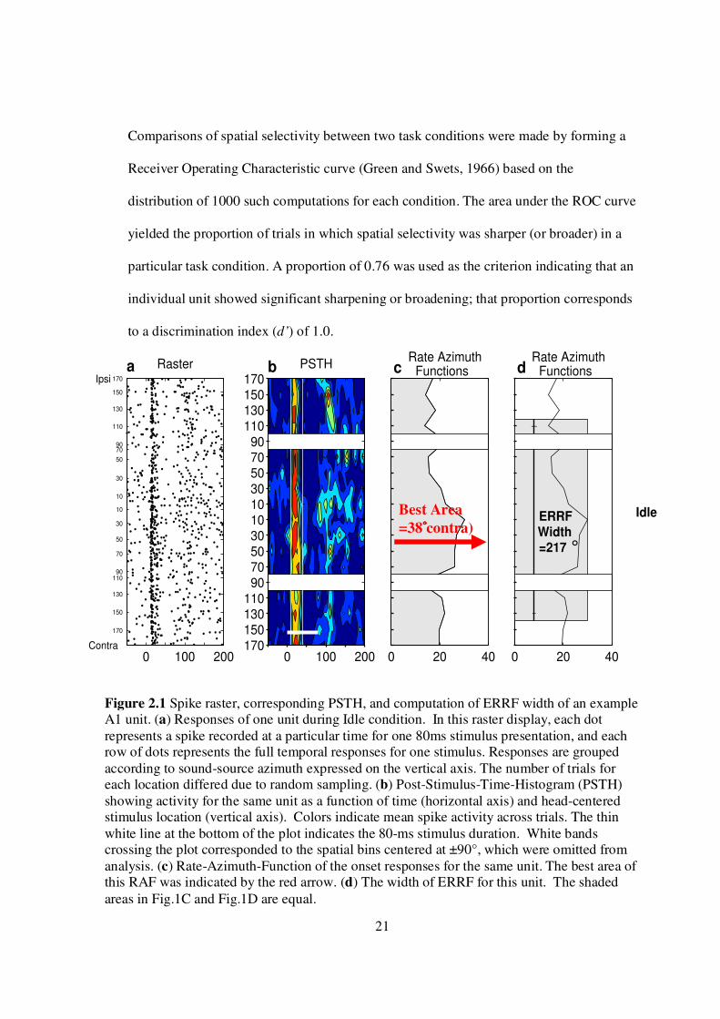
Comparisons of spatial selectivity between two task conditions were made by forming a

Receiver Operating Characteristic curve (Green and Swets, 1966) based on the

distribution of 1000 such computations for each condition. The area under the ROC curve

yielded the proportion of trials in which spatial selectivity was sharper (or broader) in a

particular task condition. A proportion of 0.76 was used as the criterion indicating that an

individual unit showed significant sharpening or broadening; that proportion corresponds

to a discrimination index (d’) of 1.0.

Figure 2.1 Spike raster, corresponding PSTH, and computation of ERRF width of an example A1 unit. (a) Responses of one unit during Idle condition. In this raster display, each dot represents a spike recorded at a particular time for one 80ms stimulus presentation, and each row of dots represents the full temporal responses for one stimulus. Responses are grouped according to sound-source azimuth expressed on the vertical axis. The number of trials for each location differed due to random sampling. (b) Post-Stimulus-Time-Histogram (PSTH) showing activity for the same unit as a function of time (horizontal axis) and head-centered stimulus location (vertical axis). Colors indicate mean spike activity across trials. The thin white line at the bottom of the plot indicates the 80-ms stimulus duration. White bands crossing the plot corresponded to the spatial bins centered at ±90°, which were omitted from analysis. (c) Rate-Azimuth-Function of the onset responses for the same unit. The best area of this RAF was indicated by the red arrow. (d) The width of ERRF for this unit. The shaded areas in Fig.1C and Fig.1D are equal.

0 100 200

170

150

130

11090

70

50

30

10

10

30

507090

110

130

150

170

Contra

IpsiRastera PSTHb

0 100 200170150130110

90705030101030507090

110130150170

0 20 40

Rate AzimuthFunctionsc

0 20 40

d

¯

-

ERRFWidth=217

Rate AzimuthFunctions

IdleBest Area=38����contra)

°

0 100 200

170

150

130

11090

70

50

30

10

10

30

507090

110

130

150

170

Contra

IpsiRastera PSTHb

0 100 200170150130110

90705030101030507090

110130150170

0 20 40

Rate AzimuthFunctionsc

0 20 40

d

¯

-

ERRFWidth=217

Rate AzimuthFunctions

IdleBest Area=38����contra)

0 100 200

170

150

130

11090

70

50

30

10

10

30

507090

110

130

150

170

Contra

IpsiRastera PSTHb

0 100 200170150130110

90705030101030507090

110130150170

0 20 40

Rate AzimuthFunctionsc

0 20 40

d

¯

-

ERRFWidth=217

Rate AzimuthFunctions

IdleBest Area=38����contra)

°

22

We adopted a method from our previous study (Mickey and Middlebrooks, 2003)

for estimating the amount of location-related information transmitted by unit responses.

Detailed description can be found in the previous paper (Mickey and Middlebrooks,

2003). Briefly, this analysis comprised three steps: (1) we divided trials into two pools of

equal size. Then we randomly drew trials from each pool and computed average

response patterns for each set; (2) we used a pattern-recognition algorithm to test the

consistency of stimulus-specific responses; (3) we computed the amount of stimulus-

related information transmitted by the pattern recognition. In the first step, we randomly

divided the set of trial-by-trial responses into two sets of equal size, A and B. However,

due to the fewer trials we obtained in these behavioral animals, the unequal number of

trials for each location after they were adjusted by the head position will bias the result of

pattern recognition. Therefore, instead of forming the averaged vector across all

available trials for each stimulus location in one half size pool as we did before (Mickey

and Middlebrooks, 2003), we drew only 8 trials to obtain mean response measures RA(α)

and RB(α). This optimal number was determined by the minimum trials per locations

across all units. Since we used fewer trials in the current study than our previous study,

the averaged spike pattern vector would contained more noise hence the performance for

the pattern recognition is expected to be lower.

The response measure consisted of a multidimensional spike density function; each

dimension corresponds to a spike probability in a particular poststimulus time bin

(Furukawa and Middlebrooks, 2002). Spike density functions were calculated by

representing the spike pattern on each trail as a series of zeros and ones at the resolution

23

of 0.1 m sec, then convolving with a Gaussian function (standard deviation: 5 ms), then

resampling using 5 ms time bins, and finally averaging across trials. Full spike patterns

consisted of spike density functions over the range of time 10–200 or 10-250 msec after

stimulus onset. To form ensemble spike patterns, the full or onset time windowed spike

patterns of two or more units were concatenated end to end. Therefore, if the spike

density function of one unit at one location had 48 5-ms time bins, the concatenated spike

density functions of 2 or 4 units at one locations would have 96 or 192 time bins and so

on. In the second step of the analysis, we performed pattern recognition on mean

response measures RA and RB similar to the probabilistic neural network described in the

previous study (Mickey and Middlebrooks, 2003). The input to the network was a

multidimensional mean response measure. The first layer consisted of a radial basis layer

of 16 units, one for each source location. The second layer, a competitive layer of 16

units, produced an output that corresponded to 1 of the 16 source locations. The weights

and biases of the radial basis layer were calculated from the mean response RA and the

corresponding source locations; after the weights and biases were assigned, input of RA

resulted in outputs YAA that corresponded to the true source locations. To characterize

how consistent RB was with RA, the mean response RB was presented to the network and

the output YAB was recorded. RA and RB were then interchanged and an output YBA was

obtained in a similar manner. The more closely that RA and RB resembled one another, the

more closely YAB and YBA estimated the true stimulus locations. To reduce noise, the

entire procedure was repeated a total of 200 times. The combination of units the

ensemble was determined randomly and each ensemble size was tested for 100 different

combinations. In the third step of the analysis, we estimated, for each unit and each

24

response measure, the average amount of information transmitted about stimulus location.

First, a 16 X16 confusion matrix was constructed from the network estimates for each

location. Element i,j of the confusion matrix consisted of the number of network outputs

at location i for the true stimulus location j. The accuracy of network estimates was

characterized by computing the mutual information (Rieke et al., 1997), i.e., the

transmitted information:

T = ∑i ∑j pij log2(pij /( pipj)).

The more closely that network outputs estimated the true stimulus locations, the greater

was T. This method of calculating transmitted information overestimates the information

in the case of random input data. For that reason we ultimately used a corrected

transmitted information Tcorr =T -T0, where T0 was determined by a control analysis, in

which the relationship between spike patterns and stimuli was randomized. In that

analysis, the trial-by-trial association of stimulus location with unit responses was

reassigned randomly. The subsequent three-step analysis was identical to that used to

determine T. Given 16 stimulus locations, Tcorr theoretically ranges from 0 to 4 bits [i.e.,

log2(16)]. We consider the estimate Tcorr to be a lower bound on the true amount of

transmitted information, because the architecture and training of the artificial neural

network were likely suboptimal in many cases.

25

CHAPTER 3

Task-Dependent Dynamics of Spatial Sensitivity

in the Primary Auditory Cortex (A1)

3.1 Introduction

In a typical auditory scene, a listener can focus auditory attention toward the

location of any target. The dynamic nature of active spatial listening has been

demonstrated by psychophysical studies showing that: localization or identification of a

target is more efficient when the target is presented at a cued or attended location

(McDonald and Ward, 1999; Mondor and Zatorre, 1995; Rhodes, 1987; Roberts et al.,

2009; Spence and Driver, 1994) ; prior knowledge of the location of a target enhances

spatial release from masking (Allen et al., 2009; Best et al., 2008; Kidd et al., 2005); and

localization judgments can be biased by a preceding distractor (Kopco et al., 2007). The

present study is a first attempt to explore cortical mechanisms that might underlie task-

dependent modulation of auditory spatial sensitivity.

26

Lesion studies and reversible inactivation have demonstrated that activity in the

primary auditory cortex (A1) is necessary for normal sound-localization behavior

(Jenkins and Merzenich, 1984; Malhotra et al., 2004). Also, A1 projects to the dorsal

zone (DZ) and the posterior auditory field (PAF) in which reversible inactivation

produces localization deficits (Malhotra et al., 2004; Malhotra et al., 2008). One might

speculate, therefore, that task-dependent modulation of activity in A1 might contribute to

dynamic aspects of spatial hearing. Single-unit studies in anesthetized animals have

demonstrated quite broad spatial tuning, with most spatial receptive fields ranging from

180° to 360° in width (Imig et al., 1990; Middlebrooks et al., 1994; Middlebrooks and

Pettigrew, 1981). Spatial tuning can be sharper in unanesthetized conditions, although the

majority of neurons still exhibit spatial receptive fields spanning more than a hemifield of

space (Mickey and Middlebrooks, 2003). We have tested the hypothesis that the spatial

sensitivity of neurons in A1 is modulated according to an animal’s behavioral state and,

specifically, that spatial tuning is sharpened when an animal is engaged in a sound-

localization task.

In the present study, cats were trained to perform two tasks. The first, Timbre

Discrimination, required that the cat attend to sounds in order to receive a food reward,

but reward was not contingent on sound location. The second task, Localization, required

that the cat evaluate the location of each sound. We recorded unit activity in A1 during

performance of both tasks as well as in Idle conditions in which the cat was not engaged

in either task. We found that the spatial tuning of many neurons sharpened significantly

during behavioral conditions, especially in Localization conditions. Several

characteristics of the spatial sharpening suggest a role for inhibitory mechanisms.

27

3.2 Results

We recorded unit activity from A1 (total N=70 units) under three behavioral

conditions: Idle, Timbre Discrimination, and Localization. In all conditions, the cat was

exposed to a background of probe sounds consisting of brief broadband noise bursts

presented at ~1.25-s intervals from varying azimuth locations in the horizontal plane. The

probe sounds served to probe the spatial sensitivity of cortical units. In the Idle condition,

there was no contingency between sound presentation and food reward. In the Timbre

Discrimination and Localization conditions, the cat initiated a behavioral trial by pressing

and holding a response key. When the cat heard a target sound, it released the key to

receive a food reward. The target sound in the Timbre Discrimination condition was a

200/s click train. In that condition, the target sound was associated with a food reward,

but the target location was irrelevant to reinforcement. The target sound in the

Localization condition was a broadband noise burst, identical to the probe sounds except

that it was presented from an elevation ≥ 40° above the horizontal plane at varying

azimuths. In that condition, the cat was forced to evaluate the location of each sound in

order to detect the elevated target. This localization was accomplished covertly, in that

the cats typically did not make orienting movements of the head or external ears towards

the sounds. The physiological recordings reported here reflect responses only to the

broadband probe sounds, not to the target sounds.

3.2.1 General characteristics of spatial selectivity and temporal firing patterns

Units responded to the probe sounds with a variety of temporal firing patterns and

spatial sensitivity. The responses of many units also varied among task conditions. We

28

quantify the task-dependent modulation of spatial sensitivity in the next section (see

3.2.2). Here we demonstrate several example units for the task-dependent modulations

(Fig. 3.1~3.3). The unit in Fig. 3.1 fired a burst of spikes after the onset of the stimulus

with little or no tonic activity following the onset burst. In the Idle condition, this unit

responded uniformly to probe sounds at all locations with little selectivity to the stimulus

azimuth (Fig. 3.1A). When the animal was engaged in the Timbre task, however, the

Figure 3.1 Task-dependant modulation of spatial sensitivity. (a) Post-Stimulus-Time-Histogram (PSTH) showing activity as a function of time (horizontal axis) and head-centered stimulus location (vertical axis) for one example unit in A1 in the right hemisphere during the Idle condition (ERRF=217°). Colors indicate mean spike activity. The thin white line at the bottom of the plot indicates the 80-ms stimulus duration. White bands crossing the plot corresponded to the spatial bins centered at contralateral or ipsilateral 90°, which were omitted from analysis. (b) PSTH of the same unit during the Timbre Discrimination condition (ERRF = 173°). (c) PSTH of the same unit during the Localization condition (ERRF = 143°). (d) Average spike rates during onset response [10~40ms] as functions of azimuth locations. Black trace plots rate-azimuth-function in Idle condition; Blue trace plots rate-azimuth-function in Timbre condition; red trace plots rate-azimuth-function in Localization condition. The data for three conditions was obtained within a single behavioral session, which lasted about 100 min.

29

responses became more selective, showing suppression of responses to stimuli from the

ipsilateral field while maintaining the responses to the contralateral stimuli (Fig. 3.1B).

In the Localization condition, the responses became even more selective, responding best

to stimuli located between -10° and -50° (Fig.3.1C).

Task-dependent changes in spatial selectivity could be replicated within single

~1.5-hr recording sessions, as in the example shown in Fig. 3.2. Responses of this unit

were largely restricted to the contralateral hemifield during the initial block of trials in the

Localization condition (Fig. 3.2A). The spatial tuning broadened during a subsequent

Idle condition (Fig. 3.2B), and then sharpened again during the second block of

Localization trials (Fig. 3.2D). Finally the responses broadened again during the last Idle

condition (Fig. 3.2E). About 63% of units in our sample (N=44) were similar to those in

Fig. 3.1 and 3.2 in that they responded primarily with a burst of spikes at stimulus onset

and were omni-directional in the Idle condition. Many of those units showed task-

dependent sharpening of the spatial sensitivity like that illustrated in Fig. 3.1 and 3.2.

About 26% of units in our sample (N=18) showed more complex temporal firing

patterns, consisting of an onset response followed by a period of suppression followed by

additional bursts of spikes. In the Idle condition, units with complex temporal firing

patterns typically showed sharper spatial selectivity than did units having only onset

responses, often with spatial tuning restricted to a hemifield. In contrast to the onset-only

units, however, units with complex firing patterns tended to show relatively smaller

difference across behavioral conditions.

30

Figure 3.2 Modulation of spatial sensitivity in sequential conditions. (a) PSTH of an example unit from the left hemisphere recorded during the first sequence of localization trials from the beginning of the recording (0 min) to first 13 minutes. (b) The same unit recorded during a subsequent idle period from 13 min to 18 min after the beginning of the recording. (c) Rate-azimuth-function of the onset responses for the first Loc (red trace) and the subsequent Idle condition (black trace). (d) A second block of localization trials was started at 25 min to 34 min after the beginning of the recording. (e) A second idle period lasted from 34 min to 39 min after the beginning of the recording. (f) Rate-azimuth-function of the onset responses for the second Loc (red trace) and the subsequent Idle condition (black trace). Plot conventions are the same as in Figure 1.

31

About 8% of the units in our sample (N=6) showed prominent offset responses,

with the ratio of offset to onset responses increasing from Idle to Timbre to Localization

conditions; examples of two units are shown in Fig. 3.3. In the Idle condition (Fig. 3.3A,

D), these units responded strongly to the stimulus onset with (Fig. 3.3A) or without (Fig.

3.3D) offset response. In the two behavioral conditions, however, the onset response

weakened or disappeared and was replaced by a strong offset response (Fig. 3.3B, C, E,

and F). Of the six units that showed strong offset responses, four showed this transition

from onset to offset when the animal engaged in the behavioral tasks. Because of the

lack of consistent excitatory responses, we did not include these units in quantitative

analysis of the task dependence of spatial tuning, nor did we include the two additional

units that showed only suppression of spontaneous activity after stimulus onset. The

~89% of units (N=62) included in the following quantitative analysis all responded with

excitation during the first 40 ms after the stimulus onset. Most of those units showed only

sparse, irregular responses at times greater than 40 ms after stimulus onset. For that

reason, we restricted further quantitative analysis to spikes falling within 40 ms after

stimulus onset.

3.2.2 Quantitative measures of task dependence of responses

We quantified the location sensitivity of units using a measure inspired by the

“Equivalent Rectangular Bandwidth” introduced by Moore and Glasberg (Moore and

Glasberg, 1983). In our case, we first computed rate-azimuth functions consisting of

mean spike rates as a function of stimulus azimuth. We then computed the area under the

rate-azimuth function and re-shaped the function to form a rectangle having equal peak

32

Figure 3.3 PSTH plots in three task conditions from two units that showed offset dominant responses. Figure a~c were PSTHs from one unit recorded across three conditions (a: Idle, b: Timbre Discrimination, c: Localization) within a 105 min session. Figure d~f were PSTHs from another unit recorded across three conditions (d: Idle, e: Timbre Discrimination, f: Localization) within a 120 min session. For each unit, the ratio of offset to onset responses increased from Idle to Timbre to Localization conditions. Plot conventions are the same as in Figure 1.

33

spike rate and equal area. The resulting width in azimuth gave the width of the equivalent

rectangular receptive field (ERRF). The ERRF widths of units were influenced both by

the widths of the units’ receptive fields and by the depths of azimuth-dependent

modulation of mean firing rates. In principle, ERRF widths could range from 20°

(responses only to one stimulus azimuth) to 320° (uniform responses to all tested

locations); the maximum possible ERRF was 320°, rather than 360°, because we omitted

responses to stimuli at ±90° azimuth, which were tested with an inadequate number of

trials.

In the idle condition, units’ spatial receptive fields were relatively broad, with

ERRF widths ranging from 100° to 270° (median= 185°). The effect of behavioral

condition on ERRF widths varied among units, but ERRF widths most often narrowed

when the animal was performing an auditory task. In the Timbre Discrimination

condition (Fig. 3.4A), ERRF widths narrowed significantly on average compared to the

Idle condition (p<0.005, t-test; Timbre median: 176°; range 98°~251°). The ERRF widths

of many units narrowed further in the Localization condition compared to the Timbre

Discrimination condition (Fig. 3.4B), but ERRF widths of other units broadened. Overall,

there was no significant difference in ERRF width between these conditions (p=0.18,

Localization median 165°; range 63° ~250°). The greatest contrast in spatial sensitivity

was seen between Idle and Localization conditions (Fig. 3.4C): median ERRF widths

narrowed from 185° to 165° (p<0.0005). Again, there was considerable variation among

units, with most units showing a substantial narrowing of ERRF widths, but others

showing no narrowing or even a slight broadening.

34

Figure 3.4 Comparisons of ERRF widths across condition-pairs for all units with excitatory responses within first 40ms after stimulus onset. Each symbol represented one unit, with the value in horizontal and vertical axes corresponding to its ERRF width in two different conditions. The symbols lying below the diagonal line represent units for which spatial tuning sharpened (and the ERRF width narrowed) for the condition indicated on the abscissa. “o” symbols represent the units that did not show significant sharpening or broadening of ERRF widths. “+” symbols represent the units that showed significant sharpening and “x’ symbols represent the units that showed significant broadening according to the bootstrap test described in relation to Fig. 3.5.

We wished to evaluate the percentage of units that showed statistically significant

sharpening or broadening of their spatial sensitivity as a function of task condition. For

that reason, we performed a bootstrapping procedure to evaluate the trial-by-trial-

variation in rate-azimuth functions of individual units. We tested for differences in

ERRF widths of individual units between various pairs of task conditions, using a

Receiver-Operating-Condition technique with criterion of d’≥1 (see Methods) for

significant sharpening or broadening of spatial sensitivity.

0 80 160 240 3200

80

160

240

320

Idle

Tim

bre

p < 0.005

a0 80 160 240 320

0

80

160

240

320

Timbre

Loca

lizat

ion

p = 0.18

b0 80 160 240 320

0

80

160

240

320

Idle

Loca

lizat

ion

p < 0.0005

c

35

The results of this analysis are shown in Fig. 3.5. In every 2-way comparison

between task conditions, more units showed a significant sharpening of spatial tuning

than showed a broadening in the condition that required greater attention to sounds

(Timbre or Localization versus Idle) or greater attention to the location of sounds

(Localization versus Timbre). As expected, the largest percentage of units showing

significant sharpening of spatial sensitivity was observed in the contrast between Idle and

Localization, in which about 44% of units showed significantly narrower ERRF widths.

The direct comparison between the Timbre and Localization conditions is especially

interesting, since the presumed levels of arousal and motor demands were identical: the

cat detected a target sound amid a sequence of background sounds and then released a

key. The only difference was that the locations of sounds were relevant to obtaining a

food reward in only the Localization condition. In this task comparison, 24% of units

showed a significant narrowing of ERRF width in the task condition requiring

localization compared to discrimination between a click train and broadband noise.

Figure 3.5 Percentage of units that showed significant sharpening or broadening of spatial tuning between condition pairs. Light bars represent the percentage of units for which the ERRF width sharpened significantly for each 2-way comparison. Dark bars represent the percentage of units for which the ERRF width broadened significantly.

20

0

20

40

60

Sharpened

Broadened

Perc

enta

ge o

f Uni

ts

Timbrevs

Idle

Localizationvs

Timbre

Localizationvs

Idle

36

Our previous studies have demonstrated that, in anesthetized animals, a

substantial proportion of stimulus-related information can be transmitted by first-spike

latencies (Furukawa and Middlebrooks, 2002), although that proportion is somewhat

smaller in awake conditions (Mickey and Middlebrooks, 2003). Here we investigated the

task dependence of spike timing. Surprisingly, median first-spike latencies for the

responses to sounds at three locations that elicited the most spikes for each unit averaged

somewhat longer in the Localization condition compared to the Idle condition (20.7 vs

18.8 ms, p<.0001) but were similar between two behavioral tasks (p=0.19, Fig. 3.6A).

The trial-by-trial standard deviation of the first spike latency of three favored locations

also was significantly higher in the Localization condition (p<0.05, Fig. 3.6B).

Idle Timbre Localization10

15

20

25

30

35**** ****

Late

ncy

(ms)

a Median First Spike Latency

Idle Timbre Localization2

4

6

8

10 *

Late

ncy

(ms)

b STD of First Spike Latency

Figure 3.6 First spike latency for favored locations was longer and more dispersed during behavioral conditions. (a) Distributions of the trial-by-trial medians of first-spike latencies for favored locations across three conditions. Analysis of variance (ANOVA) showed a significant effect of condition for the median first spike latency (p < 0.005). Differences were significant in 2-way comparison between Idle and Timbre Discrimination conditions (t test, p < 0.0001) and between Idle and Localization conditions (t test, p < 0.0001) but not between Timbre Discrimination and Localization (t test, p = 0.19) (b) Distributions of the trial-by-trial standard deviation of first-spike latencies across three conditions. Standard deviations were significantly broader in the Localization compared to the Idle condition (t test, p < 0.05) but not in the other 2 comparisons. Each box shows the upper and lower quartile and median as horizontal lines. The plus signs indicated points beyond the quartiles.

37

3.2.3 The increase in spatial sensitivity comes from suppression of responses to least-

favored stimuli.

The sharpening of spatial sensitivity observed in the behaving conditions might have

represented an enhancement of the responses to the favored stimuli or it might have

resulted from a suppression of the responses to the least-favored stimuli. We tested that

first by computing the mean spike rate across all stimulus locations for all the units with

onset dominant responses (N=62). We found a significant effect of condition for the

overall mean spike rate (p < 0.005). That mean rate was significantly lower during the

Localization compared to during the Idle condition (p < 0.001) and also slightly lower in

the Localization than in the Timbre condition (but p= 0.053, Fig. 3.7A). We then tested

whether that reduction in responses was general to all the stimuli, or whether it reflected

suppression of responses to particular stimuli. Here, we focused on those units that

showed significant sharpening of spatial tuning in the onset responses when compared

Localization v.s. Idle condition in the bootstrapping analysis in Fig. 3.5 (N=27).

Responses at “favored” or “least-favored” stimulus locations were averaged across the

three locations yielding the highest or the lowest spike counts in the Localization

condition; the same favored and least-favored locations then were used to compare across

all task conditions. There was no significant difference among task conditions for spike

rates elicited by sounds at each neuron’s favored location (Fig. 3.7B; p =.75, Localization

vs Idle). In contrast, when we compared spike rates elicited by stimuli at units’ least-

favored locations, every unit showed a lower rate in the Localization condition (Fig. 3.7C;

p < 0.0001). These results indicate that the task-dependent sharpening of spatial

38

sensitivity acts primarily by enhanced suppression of responses to stimuli located outside

of units’ favored locations.

Figure 3.7 Spike rates decreased in the Localization condition primarily for stimuli at least-favored locations. (a) Distributions of spike rates averaged across all stimulus locations for the entire population. Mean spike rates decreased significantly across task conditions (Kruskal-Wallis test, p < 0.005). (b) Mean spike rates for stimuli at favored locations showed no significant difference between Localization and Idle conditions for the units that showed significant sharpening from Localization to Idle in the analysis in Fig. 3.5 (Wilcoxon rank sum test, p= 0.74). (c) Mean spike rates for least-favored locations were suppressed significantly for Localization compared to Idle conditions (p < 0.0001) for the same subset of units.

3.2.4 Time course of task-dependent modulation of spatial tuning.

We evaluated the time course of task-dependent changes in spatial sensitivity. We

focused on least-favored stimulus locations, as in Fig. 3.7C, which showed the greatest

task-dependent modulation of spike rates. We searched for cases in which stimuli at

least-favored locations were tested either in four consecutive hit trials (see Methods)

followed by four consecutive non-hit trials (Fig. 3.8A) or vice versa (Fig. 3.8B). For the

cases that matched these criteria (N=51 hit to non-hit; N=35 non-hit to hit), we

39

normalized spike rates by the mean spike rate across the contiguous 4 hit and 4 non-hit

trials. We then examined the time course of the change of the normalized spike rates for

trials around the transition from hit to non-hit (Fig. 3.8A) or non-hit to hit (Fig. 3.8B)

conditions. The time between each presentation at a particular location averaged about 40

s; the actual interval varied among cases because of the random order of testing of

various stimulus locations. As seen in Fig. 3.8A, the normalized spike rate averaged

about 0.5 per trial for the last four hit trials and did not differ significantly among those

trials. The normalized rate for the first non-hit trial, however, showed an immediate

increase to about 1.8 spikes per trial. The mean normalized spike rate for each of the four

non-hit trials was significantly higher than the mean of all the hit presentations (p <

0.0001 to p<.01, depending on trial). Essentially the reverse was seen in the transition

from non-hit to hit condition (Fig. 3.8B). The normalized spike rate for the first three

non-hit trials each was significantly higher than the mean of the later four hit

presentations (p<0.001 to p<0.005). Interestingly, the normalized spike rate for the last

non-hit trials averaged about 0.82, which is significantly lower than the normalized spike

rate for the preceding three non-hit presentations (p < 0.05) but not significantly different

from the normalized spike rate for the following hit trials (p=0.13), as if these trials

represented a transition period in which the animal was preparing to engage in the task.

These results indicate that task-dependent changes in the spatial sensitivity of units occur

on a scale no slower than some tens of seconds.

40

1 2 3 4 5 6 7 80

0.5

1

1.5

2

2.5

3N

orm

aliz

ed S

pike

Rat

ea

1 2 3 4 5 6 7 8Trial Number

b

NonHitHit

Figure 3.8 Time course of the task-dependent modulation of the response at the least-favored locations. Hit and non-hit trials are represented by light and dark bars, respectively. (a) Normalized spike rates during four consecutive hit trials (1-4) followed by the four consecutive non-hit trials (5-8). The mean normalized spike rate for each of the four non-hit trials was significantly higher than the mean of all the hit presentations (Wilcoxon rank sum test, p < 0.0001 to p<.01, depending on trial). (b) Four non-hit trials (1-4) followed by four hit trials (5-8). Error bars showed the standard errors of the means. The normalized spike rate for each of the first three non-hit trials was significantly higher than the mean of all the hit presentations that followed (p<0.001 to p<0.005).

3.3 Discussion

The results demonstrate that the spatial sensitivity of neurons in auditory cortical

area A1 changes according to animals’ behavioral state. Many of the units sharpened

their spatial tuning (i.e. ERRF width was narrowed) when the animals were engaged in a

task (i.e., the Timbre Discrimination and the Localization conditions) compared to the

Idle condition in which, we assume, they paid little attention to the sound. Moreover,

41

about 24% of the units showed significantly sharper spatial tuning when the cats were

engaged in a task that required attention to the locations of sounds compared to the

Timbre task, in which location was irrelevant. The difference in units’ responses between

the Timbre and the Localization conditions was not likely a result of differences in

arousal or motivation, since in both conditions the animals responded to the target sounds

with appropriate releases of the response key. Changes in pinna position were not likely

the cause for sharpening of spatial sensitivity, since neurons that showed significant

sharpening of ERRF widths were recorded simultaneously with units that showed no

significant change or even significant broadening of ERRF widths. The observed changes

in spatial sensitivity were global changes in the responses to the probe sounds. Our

interpretation is that the overall spatial sensitivity of A1 neurons changes to

accommodate the demands of behavioral tasks.

Our results bear some similarities to the recent results from Fritz and colleagues

(Fritz et al., 2003; Fritz et al., 2005b), who recorded from area A1 in ferrets that were

engaged in tone-detection tasks. In those studies, spectrotemporal receptive fields (STRFs)

of cortical neurons were measured in response to broadband probe stimuli. Task-related

changes in STRFs were observed during and after task performance that resulted in

increased excitation by target frequencies and/or increased inhibition by non-target

frequencies. Those results differed from ours in that cortical STRFs reorganized around

particular target frequencies, rather than showing an overall sharpening of sensitivity

analogous to the general sharpening of ERRF widths that we observed. Also, in many

instances, the changes in STRFs reported by the Fritz group persisted for hours after

cessation of the task, whereas we observed abrupt changes in ERRF widths within the

42

tens-of-seconds time resolution afforded by our experimental design. The persistent

effect observed by Fritz and colleagues might have resulted from the aversive

conditioning paradigm that was used in their studies. The more transient effect we

observed might be a result of attentional control due to the positive reinforcement

paradigm used here. A previous study from Kopco and colleagues (Kopco et al., 2007)

reported that subjects’ sound localization performance could be biased away from a

distractor location even on interleaved baseline trials on which there was no distractor

presented. A subsequent study of the temporal characteristics of this task-dependent

contextual shift showed a similar tens-of-seconds time course. This bias reached the

maximum (or disappeared) within 90 to 120 s after the onset (or offset) of the distractor

trials (abstract # 422: Tomoriova, Andoga, Barto & Kopco, Association for Research in

Otolaryngology meeting, 2009).

We are aware of two previous studies that addressed the influence of an animal’s

behavioral state on the sensitivity of auditory cortical neurons to sound-locations (Benson

et al., 1981) or to acoustic cues to sound location (Scott et al., 2007). In the study by

Benson and colleagues (Benson et al., 1981), monkeys discriminated among sounds at

five locations. In the performing condition firing rates increased significantly in 22% and

decreased in 7% of units in A1 and other auditory cortical areas, compared to the non-

performing condition. There was no test of task-related changes in spatial sensitivity.

Similarly, Scott and colleagues (Scott et al., 2007) trained monkeys to detect the direction

of a shift in lateralization resulting from a change in interaural phase difference. In that

study, cortical neurons showed task-related changes in spike rates, most often increasing

in the on-task condition, but there was no indication of changes in sensitivity to interaural

43

phase difference. The design of those two studies differed from ours in that the responses

of interest were the responses to target sounds, whereas we measured spatial sensitivity to

non-target probe sounds. The observed enhancement of excitatory responses to the target

stimulus in these studies could coexist with our observation of global suppression at

least-favored locations. Also, we note that the previous studies tested only a limited

number of stimulus values, either 5 locations or 2 phase differences, whereas we

routinely probed 18 loudspeaker locations distributed through 360° of azimuth.

Plasticity in the functional organization of area A1 in regard to frequency

representation has been demonstrated by a number of groups, generally in association

with conditioned association (Diamond and Weinberger, 1989) or sensory discrimination

(Polley et al., 2006; Recanzone et al., 1993) paradigms. Generally, such studies have

shown increases in the responses to frequencies that were presented as conditioned

stimuli (Fritz et al., 2003). This enhancement of the representations of behaviorally

reinforced stimuli at the cortical level has been suggested to be related to cholinergic and

dopaminergic neuromodulators. Previous studies have proposed that behaviorally

relevant stimuli may activate the cholinergic or dopaminergic neurons in basal forebrain,

in addition to the sensory cortex, through a sensory cortex-to-prefrontal cortex-to-basal

forebrain circuit (Golmayo et al., 2003; Rasmusson et al., 2007). Direct electrical

stimulation of the cholinergic neurons in nucleus basalis (Kilgard and Merzenich, 1998)

and the dopaminergic neurons in ventral tegmental area (Bao et al., 2001) of basal

forebrain enhanced the representation for the paired stimuli in the sensory cortex and

thalamus (Zhang and Yan, 2008). It remains to be seen whether those same modulatory

44

systems underlie the short-term task-dependence changes in cortical sensitivity that we

have observed.

Several lines of evidence suggest that the sharpening of spatial sensitivity that we

observed during on-task conditions reflects largely inhibitory mechanisms. First, the

sharpened spatial sensitivity resulted from the suppression of least-favored responses

during the Localization condition, compared to the Idle condition. Second, in a small

number of units that showed primarily offset responses, onset responses were suppressed

resulting in increased ratio of offset to onset from Idle to Timbre to Localization

conditions. Third, the first spike latency was significantly longer and its variation was

greater during the Localization compared to the Idle condition. Inhibitory mechanisms

have been proposed to play an important role for perceptual learning in sensory cortex

(Ghose, 2004; Ohl and Scheich, 2005). An increase in inhibition has been reported to be

positively correlated with improvement of behavioral performance (Brechmann and

Scheich, 2005; Cansino and Williamson, 1997; Witte and Kipke, 2005), with increase of

task difficulty (Atiani et al., 2009) or engagement in a behavioral task that required more

global attention (Otazu et al., 2009). It has been suggested that attention or the effect of

learning may first induce change in the prefrontal cortex, which in turn activates the

GABAergic reticular nuclei in thalamus (McAlonan et al., 2006; Zikopoulos and Barbas,

2006). The reticular nuclei then will send inhibitory input to medial geniculate body

(MGB) to modulate its activity (Cotillon-Williams et al., 2008; Kimura et al., 2007) and

further change response properties in the primary auditory cortex (Ma and Suga, 2009;

Verbny et al., 2006). Temporal precision of inhibition has been shown to be important for

cortical spike timing and receptive field properties (Wehr and Zador, 2003). In the

45

present study, we observed not only a decrease in responsiveness of the A1 units during

behavioral conditions, but changes in first-spike latencies: latencies for the favored

location were delayed and exhibited more variation in the Localization condition (Fig. 3.6)

than in the Idle condition. Even in the Idle condition, the median of the first spike

latency was longer than the latency in anesthetized A1 (17.6 ms, Stecker et al., 2005a),

which is consistent with previous report (Ter-Mikaelian et al., 2007). These results

suggest that inhibitory mechanisms, driven by top-down control, could account for task-

dependent modulation of neuronal activity, either by increasing the depolarization

threshold or by delaying the spiking when the animals are engaged in the behavioral tasks.

Previous electrophysiological studies of A1 and other auditory cortical areas have

failed to identify a point-to-point map of auditory space (Imig et al., 1990; Mickey and

Middlebrooks, 2003; Middlebrooks et al., 1994; Middlebrooks et al., 1998). Instead, we

have argued that auditory space is represented in a highly distributed manner, in which

the location of any particular sound source is represented by the activity of populations of

neurons widely distributed within particular cortical areas and among multiple cortical

areas. The task-dependent modulation of spatial sensitivity observed in the present study

is also consistent with that view. The present results suggest that sound-source locations

are represented by dynamic cortical populations, the responses of which are modulated to

optimize the representation for the demands of any particular task. We have, so far, tested

only a single localization task and a single non-spatial auditory task. One might imagine

that distinct modes of spatial tuning might emerge during tasks requiring discrimination

of nearby sources, compared to tasks requiring panoramic localization, compared to

spatial stream-segregation tasks requiring segregation of multiple sequences of sounds.

46

Specific analysis of the relationship between task demands and cortical neuronal

sensitivity potentially offers a fruitful means of understanding aspects of the cortical

mechanisms of the dynamics of auditory spatial perception.

47

CHAPTER 4

Comparison of Spatial Selectivity and Temporal

Firing Patterns in A1, DZ and PAF

4.1 Introduction

The dorsal zone of the auditory cortex (DZ) in the cat is located dorsal to area A1

on the dorsal aspect of the middle ectosylvian gyrus, extending onto the ventral bank of

the suprasylvian sulcus. Although DZ initially was defined as a division of A1

(Middlebrooks and Zook, 1983), accumulating evidence indicates that DZ should be

regarded as a distinct auditory area. Anatomical tracing studies show that DZ receives its

thalamocortical input primarily from the dorsal division and rostral pole of the ventral

division of the medial geniculate body (MGB) whereas A1 receives its thalamocortical

inputs mainly from the lateral nucleus of the ventral division of the MGB ((He and

Hashikawa, 1998; Lee and Winer, 2008a; Middlebrooks and Zook, 1983). A border

between DZ and A1 can be seen in the distribution of neuronal elements by using SMI-32

immunolabeling (Mellott et al., 2010). Physiological studies under anesthetized

48

conditions showed that DZ has longer first spike latencies than A1 (He et al., 1997;

Mendelson et al., 1997; Stecker et al., 2005a). Also, DZ units usually exhibit broad,

multi-peaked frequency tuning whereas A1 units usually show sharp frequency tuning

with well-defined characteristic frequency (CF) (Middlebrooks and Zook, 1983; Stecker

et al., 2005a; Sutter and Schreiner, 1991). A previous study from our lab using

anesthetized conditions has suggested that DZ units in general have sharper spatial

sensitivity than A1 units (Stecker et al. 2005), in that there is stronger azimuthal

modulation of spike rate/latency and enhanced spatial information transmission by spike

patterns.

The posterior auditory field (PAF) in the cat is located posterior to A1 along the

caudal bank of the posterior ectosylvian sulcus of the cortex. Area PAF receives input

from ventral, dorsal, and dorsal superficial nuclei in MGB with larger inputs from dorsal

superficial and less input from ventral nuclei compared to A1 (Lee and Winer, 2008a).

Moreover, PAF receives 26% of its intracortical input from A1, the largest proportional

recipient of A1 input of any auditory field, but provides only about 10% of the cortical

input to A1 (Lee and Winer, 2008b). A recent study (Carrasco & Lomber, 2009) has

shown that the deactivation of A1 has significant effects on PAF units’ response

properties whereas no significant effect on A1 units’ response properties was observed

when PAF was deactivated. These results suggest that there might be hierarchical

processing between A1 and PAF.

Lomber and his colleagues (Malhotra et al., 2007, Malhotra et al., 2008) have

demonstrated that reversible inactivation of any one of areas A1, DZ, or PAF produces

marked deficits in performance of a sound localization task, whereas inactivation of other

49

auditory cortical areas produces no such deficits (see Chapter 1 Introduction). Those

results suggest that these three cortical areas are required for normal sound localization.

In the previous chapter we evaluated the spatial sensitivity of A1 units in awake behaving

cats. We showed that A1 units exhibit task-dependent sharpening of spatial tuning during

behavioral tasks (see Chapter 3). In the present chapter we compare the spatial

sensitivity and temporal firing patterns of units in areas A1, DZ, and PAF. Our results

demonstrate both qualitative and quantitative differences among these three cortical fields

and between awake and previously reported anesthetized conditions. To our knowledge,

this study is the first to investigate the properties of DZ and PAF in the awake conditions.

4.2 Results & Discussion

We recorded unit activity from auditory cortical area A1, DZ and PAF from five

animals (the same group of animals as in Chapter 3) under three behavioral conditions:

Idle, Timbre Discrimination, and Localization. We compared unit activities to the same

set of background of probe sounds consisting brief broadband noise bursts from varying

azimuth locations. All conditions were tested within single ~1.5hr recording sessions.

The differences in responses between Idle and the two behaving conditions were

somewhat smaller for DZ and PAF units that for A1 units. The present chapter focuses

primarily on the Idle condition, and task-dependent differences will be addressed in

Chapter 5.

4.2.1 General characteristics of spatial selectivity and temporal firing patterns in DZ

We observed a variety of temporal firing patterns and spatial sensitivity for DZ and

PAF in awake behaving conditions. For DZ, the majority of units (~60%, N=61)

50

responded to stimuli primarily with strong onset responses and little sustained (i.e., tonic)

activity, as seen in A1. A small percentage (10%, N=10) of DZ units showed either

suppression of the spontaneous activity or predominant offset responses. The remaining

~30% (N=32) of DZ units exhibited sustained response patterns and complex spatial

sensitivity. In Fig. 4.1A we show one example unit that fired location-specific onset and

tonic responses in addition to the initial onset bursts. This example unit responded with

an onset burst to the stimuli centered at the frontal midline. Followed by a period of

suppression after the onset, this unit responded tonically with the same preference to

frontal locations. Another example unit (Fig. 4.1B) showed a broadly tuned onset

response followed by a tonic response limited to stimuli near the frontal midline. In this

example, the tonic response to midline stimuli persisted for ~100 ms after the stimulus

offset. For DZ units like those in Fig. 4.1A-and B that displayed reliable tonic activity

after the onset burst, we found that their tonic responses were usually driven only by the

stimuli located within a restricted receptive field centered near the frontal midline.

The preference for frontal azimuthal locations was also evident for units that

showed primarily onset-dominant responses. An example unit shown in Fig. 4.1C fired a

transient burst of spikes within the first 50 ms after the stimulus onset only to the stimuli

located within contralateral 30° to ispilateral 30° across frontal midline, followed by little

or no tonic response during the Idle condition (Fig. 4.1C). About 60% of our sample

showed a temporal pattern similar to the example in Fig. 4.1C, in which the units

responded to favored locations with a strong onset response followed by sparse and

irregular tonic responses. The spatial tuning of these onset responses often sharpened

51

during the behavioral tasks compared to the Idle condition; task-dependent sharpening of

spatial tuning is quantified in Chapter 5.

~ 8% ~ 20% ~ 60%

Figure 4.1 DZ units showed strong preference for stimuli near the frontal midline. (A) Post-Stimulus-Time- Histogram (PSTH) showing activity as a function of time (horizontal axis) and head centered stimulus location (vertical axis; positive azimuths indicate the locations on the cat’s right side) for one example unit in DZ in the right hemisphere during the Idle condition. Colors indicate mean spike activity. The thin white line at the bottom of the plot indicates the 80-ms stimulus duration. White bands crossing the plot corresponded to the spatial bins centered at ±90°, which were omitted from analysis. This unit showed sustained firing after the initial onset responses. Both onset and tonic responses showed strong preference for frontal locations. (B) PSTH of another unit during the Idle condition. This unit had broader onset responses for contralateral stimuli but the tonic responses were more restricted to the stimuli near frontal midline. (C) PSTH of a third unit during the Idle condition. This unit showed primarily onset responses and had strong preference for locations near midline.

52

4.2.2 General characteristics of spatial selectivity and temporal firing patterns in

PAF

For PAF units, we found greater variety of temporal response pattern and spatial

selectivity compared to A1 and DZ. About 40% (N=89) of units showed primarily onset

responses with sparse or irregular tonic responses and a substantial percentage of units

(about 30%, N=62) exhibited complex-inhibitory responses. The remaining ~30% of

units showed reliable tonic responses and usually had high spatial sensitivity, similar to

tonic units in DZ. However, in contrast to the strong midline preferences of tonic units in

DZ, tonic units in PAF had best areas more evenly distributed across 360º of space. In

Fig. 4.2A to Fig. 4.2G we show seven sharply-tuned representative units, recorded in four

probe placements across four animals during Idle conditions, presented in an order

according to the ipsilateral-to-contralateral locations of their best areas. The example in

Fig. 4.2A was a unit that favored stimuli from 19º azimuth in the right hemifield, which

was ipsilateral to the recording site. Fig. 4.2B was a unit that favored stimuli near 0º

azimuth. Units in Fig. 4.2C to Fig. 4.2F had best areas for contralateral stimuli ranging

from 30º to 151º azimuth. The example in Fig. 4.2G had a best area falling into the 170º

bins, which indicated that this unit favored stimuli from the exact rear location of the

animal. Although the examples shown here exhibited a variety of temporal firing

patterns, most of them had some tonic response components following the initial burst of

spikes after the onset of stimulus. Usually these tonic responses showed higher

selectivity to the stimulus locations than did their onset responses (Fig. 4.2B~4.2F). This

is the first observation of awake cortical units exhibiting sharp tuning and sustained

activity for favored stimuli across different azimuth locations in PAF. We investigated

53

whether there is any topographical organization of these sharply-tuned units. Although

our current experimental design did not allow us to systematically map the cortex, our

present data are inconsistent with the presence of a topographical organization of spatial

tuning in PAF. That is, nearby units sometimes had widely separated best areas, and

Figure 4.2 PAF units showed best areas evenly distributed across space. (A) ~(G) PSTHs of 7 units presented in order according to the ipsilateral-to-contralateral locations of their best areas. Arrows and number indicated the best area for individual units (c: Contralateral, i: Ipsilateral). Plot conventions are the same as in Figure 1. (H) Best areas of 18 units recorded along one probe placement that were oriented approximately perpendicular to the cortical surface at one cortical site. (I) Best areas of 14 units recorded along another probe placement. The circles containing an x indicated units whose best areas were not computed because their spike rates did not vary sufficiently across location.

54

widely separated units sometimes had similar best areas. Those characteristics are

evident in Fig. 4.2H~I, which summarize the best areas of units encountered along two

multi-site probe placements that were oriented approximately perpendicular to the

cortical surface. Each placement encompassed a large range of best areas, suggesting the

absence of location-specific cortical columns. Moreover, there was no indication of

particular best areas associated with specific cortical depths (Fig. 4.2H~I).

In addition to those sharply tuned units (Fig. 4.2), we also encountered some PAF

units (~30% in our sample) that showed interesting inhibitory responses (Fig. 4.3). These

units had high spontaneous activity, and usually the spontaneous activity was suppressed

after the stimulus onset (Fig. 4.3A & B). For some units, the suppression of spontaneous

activity showed complex patterns and was somewhat location-specific (Fig. 4.3A). For

the example in Fig. 4.3A, the spontaneous activity was suppressed by the in the left

/contralateral hemifield but not in the right/ipsilateral hemifield. For other units, the

suppression of spontaneous activity did not show any spatial selectivity (Fig. 4.3B). In

some cases, PAF neurons with complex inhibitory responses were located in proximity to

neurons that showed complementary excitatory responses. The example showing in Fig.

4.4 is from a pair of nearby units from the same penetration recorded at the same session.

The unit in Fig. 4.4A had high spontaneous activity and showed azimuth-dependent

inhibition after the stimulus onset. The nearby unit showed relatively low spontaneous

activity and an excitatory response to contralateral stimulus (Fig. 4.4B). The spatial

dependence and the latency of the excitatory responses in Fig. 4.4B aligned closely with

the spatial dependence of the inhibition in the upper panel (Fig. 4.4A). These

55

complementary mirror responses of unit pair were usually more evident during

behavioral tasks.

Figure 4.3 Inhibitory responses in PAF. Two examples of PAF units that showed higher spontaneous activity that was suppressed after stimulus onset. The suppression of spontaneous activity was either (A) azimuth-dependent (complex inhibitory) or (B) general to all stimulus locations.

56

Figure 4.4 Complex inhibitory responses in PAF sometimes were accompanied by complementary excitatory responses from other units nearby. (A) One example unit showed complex inhibitory responses with high spontaneous activity which was suppressed for contralateral stimuli during the Localization condition. (B) Another unit that was recorded at the same time with the unit in upper panel at a nearby recording site (600 um apart). This pair of units showed complementary excitatory and inhibitory responses.

57

The rest of the PAF units (~40%, N=89) showed predominant onset responses

(fired a strong burst of spikes within 10~40ms after the stimulus onset) with or without

subsequent tonic firing, as three representative units illustrated in Fig. 4.5. About half of

the onset-dominant units showed little or no tonic responses after the initial onset burst

(Fig. 4.5A), whereas the other half showed some irregular and sparse tonic responses in

addition to their onset responses (Fig. 4.5B & 4.5C). In general, the majority of the PAF

onset neurons (as in Fig. 4.5A and 4.5C) showed broad spatial tuning, either responded

omnidirectionally (Fig. 4.5A and the onset responses in Fig. 4.5C) or responded to

stimuli spanning entire hemifield (Fig. 4.5B and the tonic responses in Fig. 4.5C).

Figure 4.5 Onset dominant units in PAF. (A) One example unit showed an omnidirectional onset response with little tonic activity. (B) Anther example unit showed an onset response for contralateral hemifield with some tonic responses. (C) A third example showed omnidirectional onset responses with irregular tonic activity.

58

4.2.3 Quantitative measures of spatial sensitivity: comparison across A1, DZ and

PAF.

To quantify the units’ spatial sensitivity, we first computed each unit’s best area. We

defined the unit’s best area using the spike rate-weighted centroid (see Methods), which

usually was centered at the peak of Rate-Azimuth-Function. The spike rate was averaged

over the whole recording duration (10~160ms for 80ms stimulus; 10~230 for 150 ms

stimulus) in order to capture diversity of response patterns and spatial sensitivity. In Fig.

4.6 we compared the distributions of best areas across three cortical fields. We found

that the best areas of A1 units usually scattered within the contralateral hemifield and

ipsilateral frontal space (Fig. 4.6A), which is consistent with our previous study (Mickey

and Middlebrooks, 2003). For DZ, we found that many units had best areas centered

around the frontal midline (0° azimuth, Fig. 4.6B). Interestingly, this contrasts with our

previous study of DZ under anesthetized conditions (Stecker et al. 2005a and Stecker et

al. 2005b) in which we found more DZ units that favored stimuli from contralateral

hemifield near 90°. The comparison of the distribution of the best areas for awake DZ

units (Fig. 4.6B) and awake A1 units (Fig. 4.6A) also confirmed the observation that the

preference for frontal stimuli is indeed a special property of DZ. There were more units

in DZ (47%) with best areas that fell within ±40° of the frontal midline during Idle

condition, compared to A1 (36%). Moreover, there were fewer DZ units (19%) than A1

units (33%) for which centroids were undefined, which occurred when the modulation

depths of their rate-azimuth functions were smaller than 50% .

In Fig. 4.6C we showed the distributions of the best areas in PAF. We found that

there were many units (23%) in PAF that had best areas for contralateral rear locations

59

compared to A1 (16%) or DZ (13%). There were also more PAF units (10%) that favored

ipsilateral rear locations than DZ (8%) whereas there were no A1 units whose best areas

fell into the ipsilateral rear quadrant. When compared to our previous study in

anesthetized animals, we found that overall there were also more units in awake PAF that

favored ipsilateral locations (21%) than were found in anesthetized PAF (15%, Stecker

et al., 2005). These results indicated that distribution of the best areas of PAF was more

uniformly distributed across 360° of space than for DZ, A1 units, or PAF units in

anesthetized animals.

Figure 4.6 Comparison of best areas across three cortical fields. The spatial distribution of best areas in each field is represented by a “rose plot” in which the area of each petal represents the percentage of units with best areas centered at the corresponding azimuth. (A) Area A1. (B) Area DZ. (C) Area PAF.

60

We further characterized spatial sensitivity in three cortical areas by measuring the

tuning width of the Equivalent Rectangular Receptive Field for individual units (see

Chapter 3). We computed the ERRF widths based on a rate-azimuth-function computed

from the averaged spike rate over the whole recording duration during Idle condition.

The accumulated distributions of the widths of ERRF widths are plotted in Fig. 4.7. We

found that overall the ERRF width in DZ was significantly sharper than PAF (p <0.05)

and A1 (p<0.005) whereas there was no overall difference in ERRF width between A1

and PAF (p=0.24). (DZ median ERRF width: 206° ; PAF median ERRF width: 221° ; A1

median ERRF width: 225° ). However, we found that there were more PAF units (17%)

Figure 4.7 Accumulated distributions of ERRF widths. The ERRF widths here were computed from average spike rate across whole recording duration for three cortical fields. Traces indicate the accumulated distribution of ERRF widths of units in their respective cortical fields. The symbols indicate the median of each distribution.

61

whose ERRF width was smaller than a hemifield (<160) than in A1 (11%). Furthermore,

DZ had the most units whose ERRF widths were smaller than a hemifield (~20%). The

larger number of units with ERRF widths smaller than a hemifield in area DZ compared

to areas A1 and PAF was due primarily to the population of DZ units with receptive

fields restricted around the frontal midline, which could be seen in Fig. 4.8B. In Fig. 4.8

we compared the relationship between individual unit’s best area and the ERRF width.

We found that majority of A1 units were broadly tuned (Fig. 4.8A). The sharply-tuned

units in DZ (smaller ERRF width) most often had best areas near the frontal midline (0°

azimuth, Fig. 4.8B) whereas the sharply-tuned units in PAF showed widelydistributed

best areas (Fig. 4.8C). The sharply-tuned units in DZ and PAF usually showed location-

specific tonic responses (see Fig. 4.1A~B and Fig. 4.2).

Figure 4.8 Comparison of best areas v.s. ERRF width across three cortical fields. (A) Area A1. (B) Area DZ. (C) Area PAF. The dash lines were drawn across ERRF width =180. NC stands for “no centroids”, in that the best areas of those units were not computed because their spike rate of that unit did not vary sufficiently across locations.

62

We further focus on the units in DZ (~30%) and in PAF (~30%) that had reliable

tonic responses. Their tonic spike rates (calculated during the 40ms after onset of

stimulus to the end of stimulus duration (80ms or 150ms); see Chapter 2 Methods)

usually comprised more than 75% of the overall spike rate (computed from 10~160ms for

80ms stimulus or 10~230ms for 150ms stimulus; see Methods). For these tonic units, we

found that their tonic responses usually were more selective for spatial location than their

onset responses (see example of DZ in Fig. 4.1B; PAF in Fig. 4.2C, 4.2E, 4.2F). We then

studied the selectivity of these tonic responses quantitatively in DZ and PAF and

compared the change of the spatial selectivity between the initial onset responses to the

tonic activities. We did not consider A1 units for the following analysis since majority of

the A1 units only had phasic responses after stimulus onset or offset, with sparse and

irregular tonic responses during the stimulus presentation. In Figures 4.9 & 4.10 we

estimated the spatial sensitivity of these tonic responses by computing the best areas and

the ERRF widths based on their tonic responses within 40 ms to 80 ms (for 80 ms probe

stimuli) or within 40 ms to 150 ms (for 150ms probe stimuli) after onset. For DZ, we

found that these tonic responses all showed strong preference for the stimuli near frontal

midline (Fig. 4.9B, also see the example in Fig. 4.1). For PAF, we found that the best

areas of these tonic responses were well distributed for locations from the contralateral

hemifield with a minority of units preferring ipsilateral stimuli (Fig. 4.9E). When we

compared the best areas computed from the onset responses (Fig. 4.9A) to the best areas

computed from the tonic responses (Fig. 4.9B) for these tonic units in DZ, we found that

they all showed similar preferences for frontal locations (Fig. 4.9C). However, in PAF,

we found that there are some units whose best areas fell in the ipsilateral hemifield during

63

the onset response and shifted to the contralateral hemifield during the tonic response

(Fig. 4.9F, i.e. points in the lower right quadrant) but not vice versa (points in the upper

left quadrant). This suggested that the spatial sensitivity might be broader for the onset

responses than their tonic responses. Indeed, when we compared the ERRF widths of the

tonic responses to the onset responses in these DZ and PAF tonic units during Idle

conditions, we found that the ERRF widths of tonic responses are significantly narrower

Figure 4.9 Best areas for tonic units in DZ and PAF. Distribution of best locations of the (A) onset responses or (B) the tonic responses of DZ tonic units. (C) Direct comparison of best areas across onset and tonic responses for each DZ tonic units. Distribution of best locations of the (D) onset responses and the (E) tonic responses for the tonic PAF units. (F) Direct comparison of best areas across onset and tonic responses for each PAF tonic unit. Plot convention is the same as Fig. 6.

64

than the ERRF widths of onset responses during Idle condition (p< 0.001; DZ: Fig. 4.10A

2nd v.s 3rd column; p< 0.0001; PAF: Fig. 4.10B, 2nd v.s.3rd column). When we compared

these tonic units with the onset-dominant units (non-tonic units) in DZ, we found that the

onset ERRF widths were comparable between two groups (p= 0.69; Fig. 4.10A 1st v.s 2rd

column). However, for PAF, we found that the onset ERRF widths of the PAF tonic

units were significantly sharper than the onset ERRF widths of the PAF units that showed

onset-dominant responses (p< 0.0001; Fig. 4.10B 1st v.s 2rd column). These results

suggested that, for this subset of PAF units that have reliable tonic responses, their onset

responses are usually broad, but somewhat sharper than units with onset-dominant

responses. After the initial transient onset responses, these tonic units became even more

selective to the stimuli. Only sounds from their favored locations could drive these units

to fire in a sustained manner, consistent with the tonic units in DZ.

Figure 4.10 Onset v.s. Tonic ERRF widths for tonic units in DZ (A) and PAF (B). Distributions in comparison are indicated on the x-axis. The pair-wise comparison showed that the ERRF widths were significantly narrowed in tonic responses compared to the onset responses in tonic units and non-tonic units for both fields. (p< 0.0001,Wilcoxon rank-sum test). The ERRF widths of the onset responses of tonic units in PAF are also significantly sharpened than onset responses in non-tonic units (Wilcoxon rank-sum test, p< 0.0001). Each box shows the upper and lower quartile and median as horizontal lines.

65

4.2.4 Comparison of first spike latency between awake and anesthetized conditions

Previous studies (Chapter 3 and Ter-Mikaelian et al, 2007) have shown that the

median first spike latency in awake A1 was longer than latencies measured in A1 of

anesthetized animals. In agreement with previous results, we found that the median of

first spike latencies of A1 across locations in our awake animals (19.6 ms) indeed were

longer than in anesthetized animals (17.6 ms, Stecker et al., 2005). Similarly, the median

first spike latencies of DZ in awake (25.8 ms) were longer than anesthetized animals

(22.0 ms, Stecker et al, 2005). Surprisingly, median first spike latencies were actually

shorter (25.0 ms) in area PAF under awake conditions than we previously observed in

PAF under anesthetized conditions (28.9 ms).

Previous studies of PAF in anesthetized animals have shown that the first spike

latency in PAF was substantially longer than A1 or DZ (Stecker et al., 2003, Stecker et al,

2005). Nevertheless, the data presented here suggest that, in awake conditions, the

latencies in A1 and DZ are much longer than in anesthetized conditions, reducing the

difference in the median first spike latency across three fields (Fig. 4.11A) (Awake A1:

23.67 ms, DZ:27.83 ms, PAF: 27.63 ms; compared to anesthetized conditions A1: 17.64

ms, DZ: 22.04 ms, PAF: 28.75 ms). The median first spike latencies in awake PAF and

DZ were significantly longer than awake A1 (p < 0.0001) but there was no significant

difference between these two non-primary fields. However, the current observations of

the latencies distribution across three fields were still consistent with the anatomical

evidence for the interfield connections and the hierarchical relationships between these

three fields (see Fig. 1.1 in Chapter 1 Introduction): units in PAF responded with longer

66

latencies might receive input from A1 units, which responded with shorter latencies; units

in DZ also responded with longer latencies, which might receive inputs from A1 and PAF.

The variation in first spike latency as a function of stimulus location reported in

previous studies in anesthetized animals was significantly greater in areas PAF (10.62 ms)

and DZ (8.38 ms) than in area A1 (3.11 ms, p < .0002). These results led to the argument

that the temporal response pattern in PAF and DZ might carry more spatial information

than is the case in A1 (Stecker et al., 2003; Stecker et al., 2005). However, an overall

comparison indicates that there were no significant differences in the variation of first

spike latency across locations among these three cortical fields in awake animals

(p>0.18). In the awake condition we found that the variations in first spike latency across

azimuth locations were much larger across all three cortical fields than previously

reported for anesthetized conditions. (A1: 14.54 ms; DZ: 15.34 ms; PAF: 15.47 ms, Fig.

4.11B).

The results above from comparisons of first spike latency between awake and

anesthetized conditions suggested that anesthesia might have differential effects on spike

latencies in different cortical fields, with first spike latencies shortened more in A1 and

DZ than PAF. Also, the previous observation of larger latency variation across locations

in anesthetized PAF (Stecker et al., 2003) might be a result of anesthetic artifacts. Alpha-

chloralose, as used in the previous studies, has been suggested to suppress neuronal

activity (Collins et al., 1983; Dimnikova, 1991; Serkov et al., 1974) and to increase the

duration of the inhibitory postsynaptic potentials of cortical neurons (Serkov et al., 1974).

67

4.3 Summary

In this chapter we described the spatial sensitivity and the temporal response

patterns of units in three cortical fields (A1, DZ and PAF) during Idle conditions. Many

units showed phasic onset responses, especially in A1. We found that there was a subset

of units in DZ and PAF that exhibited reliable tonic responses. Those tonic units in DZ

and PAF were usually more spatially selective than the ones that only showed onset-

dominant, phasic responses. Their tonic responses usually were driven only by their

favored stimuli. There was also a substantial number of PAF units that exhibited

Figure 4.11 First spike latencies in A1, DZ and PAF. (A) Distributions of the median of first spike latency computed for each unit across locations. (B) Distributions of the range of first spike latency across azimuth (∆ L = Lmax – Lmin) for each unit. Distributinos are plotted as the proportion of units per 5 ms time bin. The symbols represented the median value of the populations for each cortical area.

68

complex inhibitory responses. They usually had high spontaneous activity and the

spontaneous activity usually was suppressed after the stimulus onset.

Overall, we found that A1 units were broadly tuned for stimulus location, mostly

with receptive field larger than a hemifield. Most of the A1 units favored stimuli in

contralateral hemifield or ipsilateral frontal space. Although PAF units were not

significantly sharper than A1 on average, there was a subset of PAF units that showed

sharp spatial tuning, with ERRF widths smaller than a hemifield and best areas evenly

distributed across 360° of space. DZ units were on average sharper than A1 and PAF, due

to a subset of units which were sharply-tuned and favored stimuli restricted around the

frontal midline. The demonstration of a bias in spatial tuning of DZ units to near-midline

locations contrasts with the observation under anesthetized conditions of a bias toward far

contralateral locations (Stecker et al., 2005).

We found that overall the first spike latencies in A1 and DZ were longer in the

awake condition than in the anesthetized condition. However, first spike latencies in

awake PAF were shorter than the anesthetized condition. The differences in the first

spike latency across cortical fields were smaller in the awake condition than in the

anesthetized condition. The variation in first spike latency across spatial location also

was greater in the awake condition than in the anesthetized condition for all areas. In

contrast to the anesthetized condition, the variation in first spike latency across azimuth

locations was similar in all three areas.

69

CHAPTER 5

Task-Dependent Modulation of Spatial Sensitivity in A1, DZ and PAF

5.1 Introduction

In our previous study we have shown that the spatial sensitivity in A1 units

exhibited task-dependent modulation (Chapter 3). We found that units in A1 became

more selective for stimulus location when the animals were engaged in the behavioral

tasks compared to the Idle conditions. Many A1 neurons reduced their spatial receptive

fields from omnidirectional to hemifield by suppressing their responses to least-favored

stimuli (see Fig. 3.7 in Chapter 3). The spatial tuning further sharpened when we

compared Localization to Timbre Discrimination conditions. These adaptive changes of

receptive field properties have also been shown in the frequency responses for A1.

Previous electrophysiological studies in awake behaving ferrets have demonstrated that

the spectrotemporal receptive field of A1 neurons will change adaptively according the

behavioral task demands (Fritz et al., 2003; Fritz et al., 2005). However, the effect of

behavioral status on response properties of the units in non-primary or secondary auditory

70

cortices has not been studied yet. Studies in the visual modality have shown that

attention modulates responses of neurons throughout the visual cortices (Connor et al.,

1997; Reynolds and Chelazzi, 2004; Womelsdorf et al., 2008). Brain imaging studies of

auditory cortices (Petkov et al., 2004; Woods et al., 2009) have shown that attention

might have different effects on core versus belt auditory areas.

In this chapter, we investigated the task-dependence of the spatial sensitivity and

temporal firing patterns in areas DZ and PAF (from the same group of animals that were

studied in Chapter 3 and 4). Previous studies in anesthetized animals have suggested that

DZ and PAF might be part of the “belt” area that surrounding the “core” primary cortices.

In the previous chapter we have demonstrated qualitative and quantitative differences in

response patterns and spatial sensitivity between A1, DZ and PAF under baseline or Idle

conditions. A demonstration of how attention modulates the spatial tuning in DZ and

PAF might help us to understand their roles in processing spatial information. Our

results suggested that, while the spatial tuning is sharper in DZ and PAF than A1, task-

dependent modulations of the spatial sensitivity generally were smaller in DZ and PAF.

For the subset of units in DZ and PAF that showed reliable tonic responses, the

selectivity of stimulus location remained high in DZ and PAF units even during the Idle

condition.

5.2 Results and Discussion

The task-dependent sharpening of spatial tuning in onset responses of A1 units has

been shown in Chapter 3 (see Chapter 3, Fig. 3.1A~C). This sharpening of spatial

sensitivity of onset responses during behavioral tasks was also common for DZ and PAF

71

units. An example unit from DZ is shown in Fig. 5.1A~C. In the Idle condition, that unit

fired a transient burst of spikes predominantly within the first 50ms after the stimulus

onset, in response to sounds throughout the contralateral hemifield (Fig. 5.1A). When the

animal engaged in the Timbre Discrimination condition, however, the unit’s onset

responses became more selective and restricted to the stimuli around frontal midline (Fig.

5.1B). This unit showed the same midline-tuning during the Localization condition (Fig.

5.1C). Previously we have shown that a subset of DZ units (30%) exhibited reliable

tonic responses also showing restricted spatial sensitivity for stimuli near frontal midline.

In Fig. 5.1D~F we showed the PSTHs across three conditions for one example DZ unit

that fired location-specific tonic responses in addition to the initial onset bursts. During

the Idle condition, this example unit favored locations near frontal midline and responded

to the stimuli first with an onset burst, then a period of suppression after the onset,

followed by a tonic response that also showed preference for frontal stimuli. During the

Timbre Discrimination and Localization conditions, this unit showed similar frontal

tuning but the responses became more sustained due to a decrease of suppression after

onset burst (Fig. 5.1E and 5.1F). Another example unit (Fig. 5.1G~I) showed a broader

onset response followed by a tonic response driven only by the stimuli near frontal

midline. Similar to the previous example, the tonic activity was higher during the

behavioral conditions (Timbre Discrimination and Localization, Fig. 5.1E & 5.1F) while

the selectivity for the frontal locations remained.

In Fig 5.2 we illustrate the PSTHs across three conditions for the PAF units with

location-specific tonic responses. An example PAF unit in Fig. 5.2A~C preferred stimuli

from frontal midline (0 º azimuth). As seen in tonic DZ units, the selectivity for stimulus

72

Figure 5.1 Three example DZ units in Idle (A, D, G), Timbre Discrimination (B, E, H), and Localization conditions (C, F, I) . An example unit (A)~(C) showed sharpening of spatial tuning for its onset responses. Another example unit (D)~(F) was a unit whose onset and tonic responses all showed a preference for frontal locations. The tonic responses were more sustained during behavioral tasks. The example unit in (G)~(I) showed a broad onset response followed by a more selective tonic response with a preference for frontal midline stimuli. The tonic activity also increased during behavioral tasks. The data for three conditions was obtained within a single behavioral session. Plot conventions are the same as in Figure 1 in Chapter 3.

73

location did not change across behavioral conditions, but the tonic responses became

more sustained during the behavioral conditions. For another PAF unit that showed a

preference for the stimuli around 20 º ~30 º near frontal midline (Fig. 5.2D~F), an

additional preference was observed for the stimuli from some rear locations, especially

during the Idle condition (Fig. 5.2D), as if this unit exhibited front-back confusions that

human subjects often experience. However, the ratio of the responses of the back to the

responses of the front gradually decreased with the increase of the animal’s spatial

attention from Idle to Timbre Discrimination to Localization (Fig. 5.2E & 5.2F). The

other example PAF unit shown in Fig. 5.2G~I exhibited broadly-tuned onset responses

followed by more selective tonic responses during Idle condition (Fig. 5.2G).

Nevertheless, the onset response sharpened when the animal was engaged in the

behavioral tasks whereas the selectivity of the tonic responses did not show significant

change across conditions (Fig. 5.2G~I), a common observation in other PAF units with

this response pattern.

5.2.1 Quantitative measures of task dependence of responses across three cortical

fields: best area

To investigate the behavioral modulation of the spatial sensitivity across three

cortical fields, we first compared the best areas computed by the averaged spike rate

across the whole recording duration in Idle condition to Localization condition to see if

neurons change their preference for stimulus location when animals pay more spatial

attention (Fig. 5.3). In general, we did not observe any systematic change of best areas

across behavioral conditions in any cortical field. For instance, in Fig. 5.3C we compared

74

Figure 5.2 Three example PAF units with azimuth-dependent tonic responses in Idle (A, D, G), Timbre Discrimination (B, E, H), and Localization conditions (C, F, I) . The activity during the Idle condition for these three units have been shown in the first three PSTHs in Fig. 2 of Chapter 4. The unit in (A)~(C) showed sharp spatial tuning with best areas around 19° at the ipsilateral hemifield. Another unit in (D)~(F) showed restricted selectivity for best areas around 12° in the contralateral hemifield with increased tonic activity during behavioral tasks. The third unit in (G)~(I) had broader onset but more selective tonic responses with a best areas of ~ 30° in the contralateral hemifield. Plot conventions are the same as in Figure 1 in Chapter 3.

75

the best areas of individual PAF units for Localization (ordinate) and for Idle (abscissa)

condition. We found that many data points were clustered near the diagonal, which

indicated those best areas were consistent across the condition pair. In DZ, units whose

best areas were centered across frontal midline (Fig. 5.3D & 5.3E) usually did not change

their preference across behavioral conditions (p=0.88, Fig. 5.3F) either. For A1, there

were more units with sufficient variation of spike rate across locations to compute the

best areas during Localization conditions than Idle (Fig. 5.3I, fewer N.C. in Loc

compared to Idle). Although slightly more units’ best areas fall within ipsilateral and

contralateral 40° of frontal midline in A1 during the Localization condition (A1: 40%,

Fig. 3H) than the Idle condition (A1: 36%, Fig. 5.3G), overall there was no significant

difference between the distributions of best areas across behavioral conditions in A1

(p=.40, Wilcoxon rank sum test, Fig. 5.3I).

There is a subset of PAF units (~30%) that showed complex inhibitory responses

(see the example units in Chapter 4, Fig. 4.3 & 4.4). This type of unit usually exhibited

high spontaneous activity which was suppressed after stimulus onset. Interestingly, unlike

many onset-dominant units that showed suppression of responses to the ipsilateral stimuli

without significant change for the contralateral responses, we observed a suppression of

the spontaneous activities for contralateral stimuli with an enhancement for ipsilateral

stimuli for some of these units with complex inhibitory responses during behavioral tasks

(Fig. 4.3A in Chapter 4). We further investigated whether the contrast between

responses to ipsilateral and contralateral stimuli were also modulated by animals’

behavioral status. We found that when the animal engaged in the behavioral tasks, the

ratio of the spike rate elicited by ipsilateral locations to the spike rate elicited by

76

Figure 5.3 Comparison of best areas in Idle (A, D, G) versus Localization (B,E.H) conditions across three cortical areas. The spatial distribution of best areas in each field is represented by a “rose plot” in which the area of each petal represents the percentage of units with best areas centered at the corresponding azimuth. The right column contains scatter plots directly comparing the best areas in the Localization and the Idle conditions for individual units in PAF (C), DZ (F), and A1 (I). The blue dotted lines indicate the frontal midlines in each condition, while the red lines indicate the range spanning 40 degrees from the frontal midline in either direction. NC stands for “no centroids”, in that the best areas of those units were not computed because their spike rate of that unit did not vary sufficiently across locations. A1: 33% of units with N.C. in Idle conditions but only 26% of units with N.C. in Localization conditions; DZ: 19% of units with N.C. in Idle conditions and about the same percentage (18%) of units with N.C. in Localization conditions; PAF: 33% of units with N.C. in both Idle conditions and Localization conditions.

77

contralateral locations was significantly higher for these CI units (p <0.005, t-test) when

compared to Idle conditions (Fig. 5.4). That is, responses of these units to contralateral

stimuli were relatively suppressed during the task performance. That can be viewed as an

opposite effect of what we have observed in units with typical excitatory responses (Fig.

4.4 in Chapter 4).

5.2.2 Quantitative measures of task dependence of responses across three cortical

fields: onset activity

Our earlier study (Chapter 3) showed that units in A1 showed strong task-dependent

modulation of spatial sensitivity in their onset responses (Fig. 3.1 and Fig. 3.4 Chapter 3).

The majority of DZ units (89%, N=88) in our sample reliably fired a burst of spikes

Figure 5.4 Ipsi-Contra Ratio was higher during localization tasks for CI units. The distributions of the ratio of the spike rates elicited by ipsilateral and contralteral locations are plotted for Idle and Localization conditions. The Ipsi-Contra spike ratio for CI units was significantly higher when animals were engaged in the behavioral tasks (t-test, p<0.005). We only showed the comparison of Loc versus Idle here.

78

within 50 ms of the stimulus onset. About 70% (N=156) of the PAF units in our sample

responded to the stimulus consistently with strong onset responses. The rest of the PAF

units that did not have clear onset responses usually were the ones that showed complex

inhibition (Fig. 4.3 in Chapter 4). Therefore, we first computed the ERRF widths based

on the activity during the first 50ms after the stimulus onset for all units that had onset

responses. We compared the onset ERRF widths across three behavioral conditions for

A1, DZ and PAF in Fig. 5.5. In each of the three fields, we found that the onset ERRF

widths showed significant sharpening when the animal was engaged in the behavioral

tasks (Timbre Discrimination and Localization) compared to the Idle condition (t-test: p <

0.001 or smaller) while the ERRF widths between two on-task conditions were not

significantly different. Nevertheless, when we compared Localization with Idle condition,

the overall changes of ERRF widths in DZ and PAF across behavioral task was

Figure 5.5 Onset ERRF widths across behavioral conditions in A1 (A), DZ (B), and PAF (C). The distributions of onset ERRF widths calculated from onset responses is plotted for Idle, Timbre and Localization conditions.

79

somewhat smaller than in A1: the median ERRF widths were narrowed from 185° to

165° in A1 whereas the median ERRF widths were narrowed from 173° to 159° in DZ

and the median ERRF widths were narrowed from 197° to 185° in PAF (Fig. 5.5).

We then quantified the percentage of units that showed statistically significant

sharpening or broadening of their spatial sensitivity between condition pairs by

performing a bootstrapping procedure to evaluate the trial-by-trial variation in rate-

azimuth functions of individual units in the three cortical fields (Chapter 3). As expected,

we found that there were more units that showed significant sharpening of spatial tuning

than showed broadening when comparing behavioral tasks (Timbre Discrimination and

Localization) to Idle conditions. This was a consistent result in all three fields (Fig. 5.6):

when we compared Timbre Discrimination with Idle condition, more units showed

significant sharpening (A1: 27%; DZ: 35%; PAF: 26%) than showed significant

broadening (A1: 5%; DZ: 11%; PAF: 9%); the biggest effects of the behavioral

modulation were found when we compared Localization to Idle condition, since many

units showed significant sharpening of spatial tuning (A1: 44%; DZ: 35%; PAF:31%)

whereas relatively few units showed significant broadening of spatial tuning (A1: 5%;

DZ: 5%; PAF: 12%). However, when we compared the two behavioral conditions

(Localization v.s. Timbre Discrimination), only A1 and PAF showed more units that

were significantly sharpened (A1: 24%; PAF:22%) than broadened (A1: 10%; PAF:14%).

These results again suggested that the task-dependent modulation of spatial tuning was

stronger in A1 than in PAF or DZ.

We also investigated the source of this task-dependent sharpening of spatial tuning.

In our previous study in A1 we have shown that the narrowing of onset ERRF widths

80

during behavioral conditions resulted from the suppression of responses to the least-

favored stimuli but not from an enhancement of responses to the favored stimuli. In Fig.

5.7, we present spike rates for the subset of neurons that showed significant narrowing of

their onset ERRF widths. For neurons in the 3 fields that showed significant narrowing of

their onset ERRF widths, we compared spike rates elicited by favored and least-favored

stimuli between behavioral conditions. As we have seen previously for area A1, onset

responses of DZ and PAF neurons to favored stimuli showed no significant difference

between Idle and Localization conditions (Fig. 5.7A, B, C), whereas onset responses in

all three fields to least-favored stimuli were significantly suppressed (p < 0.001 or smaller;

Wilcoxon rank sum test; Fig. 5.7D, E, F).

Figure 5.6 Percentage of units that showed significant sharpening or broadening of spatial tuning between behavioral condition pairs in A1 (A), DZ (B), and PAF (C). Light bars represent the percentage of units for which the ERRF width sharpened significantly in each 2-way comparison. Dark bars represent the percentage of units for which the ERRF width broadened significantly.

81

Figure 5.7 The sharpening of spatial tuning in the onset responses resulted from suppression of spike rates for least-favored locations. Each data point represents the spike rate for one unit for either their favored or least-favored locations in the Localization or the Idle condition Favored locations for individual units was defined by the three locations that elicited highest spike rates, whereas least-favored locations was defined by the three locations that elicited lowest spike rates, see Chapter 3. The data presented here were those units that showed significant sharpening in Fig. 5.6.

82

5.2.3 Quantitative measures of task dependence of tonic activity

About 30% of the DZ and the PAF units had reliable tonic responses (Fig. 5.1 & Fig.

5.2). For those tonic units, tonic activity was usually more spatially sensitive than their

onset response, as we have shown in Chapter 4 (Chapter 4, Fig. 4.9& 4.10). Here we

investigated the task-dependent modulation of the spatial sensitivity for these tonic

responses in tonic units. First we found that for tonic activity, the best response areas

showed no systematic change in either DZ or PAF units when we compared Localization

and Idle conditions (Fig. 5.8A, 5.8B).

Figure 5.8 Best areas of tonic responses in DZ (A) and PAF(B) between Idle (x-axis) versus Localization (y-axis) conditions. The plotting conventions were the same as in Fig. 3.

83

We then compared the spatial tuning of tonic activity across behavioral conditions.

First, we found that the ERRF widths of these tonic responses did not show significant

sharpening during the behavioral conditions (Fig. 5.9 C & Fig. 5.9F) as the onset

responses in tonic units or non-tonic units do (Fig. 5.9A~B & Fig. 5.9D~E). These

results are consistent in both DZ and PAF. However, although the selectivity for

stimulus location did not change across conditions for these tonic units, the spike rates of

the tonic responses were significantly higher for their favored stimuli during the

Localization condition, compared to the Idle condition for both cortical fields (Fig. 5.10A

& Fig. 5.10B); this is contrary to the situation for the onset responses, shown in the

previous section.

Figure 5.9 Onset and Tonic ERRF widths for tonic units in DZ (A~C) and PAF (D~F). The change of tonic ERRF widths of tonic units was plotted in (C) and (F), compared to the change of onset ERRF widths for tonic units across three behavioral conditions in (B) and (E). The change of onset ERRF widths for onset-dominant units (non-tonic units) across behavioral conditions also showed in (A) and (D).

84

5.2.4 Task-dependent modulation of first spike latencies

Previously we observed a strong effect of behavioral conditions to the median first

spike latencies in A1 units (Chapter 3): the median first spike latencies were significantly

longer (Fig. 5.11A) and the trial-by-trial variations of the median first spike latency were

greater (Fig. 5.11D) for the favored stimuli during the behavioral conditions. Here we

examined this effect in the populations of DZ and PAF units. In general, the results from

DZ and PAF were consistent with the observation in A1: the median first spike latencies

of the favored locations in DZ and PAF were also significantly longer during behavioral

conditions (Timbre Discrimination: DZ: 21.87ms and PAF: 24.1ms; Localization: DZ:

23.10ms and PAF: 24.3ms), compared to the Idle conditions (Fig. 5.11B~C, DZ: 21.38

Figure 5.10 The spike rates of the tonic responses for the favored stimuli increased significantly during the Localization conditions compared to Idle conditions (DZ: A; PAF:B).

85

ms and PAF: 21.61ms; t-test, p< 0.0001). The median first spike latency did not differ

between the Timbre and Localization conditions for either DZ or PAF (p=0.14, p=0.29,

respectively). The variation in median first spike latencies at favored locations in DZ and

PAF was also significantly higher during the Localization condition (Fig. 5.11E, DZ:

6.81 ms; Fig. 5.11F, PAF: 9.32 ms), compared to the Idle condition (DZ: 6.39 ms; PAF:

8.43 ms; p < 0.005, t-test). In addition, the median first spike latency of the favored

locations in DZ and PAF was significantly higher than in A1 (p<0.0001). Furthermore,

PAF displayed significantly higher variation in the first spike latency than DZ or A1 (p<.

0.0001, Wilcoxon rank sum test).

5.3 Summary

In this chapter we compared the task-dependent modulation of the responses in three

cortical fields. In general, we did not observe any systematic change of the location of

best areas across behavioral conditions. However, we often observed that spatial tuning

(or the ERRF widths) was sharpened during behavioral tasks compared to Idle in any of

the cortical fields. Moreover, we found that A1 showed the strongest task-dependent

modulation of spatial sensitivity among the three cortical fields. The ERRF widths in A1

narrowed more in Localization than they did in DZ or PAF when compared to Idle

condition. When comparing the two behavioral conditions (Timbre Discrimination v.s.

Localization), only A1 showed further sharpening of spatial tunings whereas the DZ and

PAF showed comparable spatial sensitivity under both behavioral tasks. There were also

more units that showed significant sharpening in A1 than in DZ or PAF in any two-way

comparison of the ERRF widths across trials. This increase in spatial sensitivity resulted

86

from the suppression of responses to least-favored stimuli but not from the enhancement

of responses to the favored stimuli.

Figure 5.11 Behavioral modulation of first spike latency in A1 (A, D), DZ (B,E), and PAF(C, F). (A~C) Distributions of the trial-by-trial medians of first-spike latencies for preferred locations across three conditions. Differences were significant in the 2-way comparisons between Idle and Timbre Discrimination conditions and between Idle and Localization conditions but not between Timbre Discrimination and Localization. (D~F) Distributions of the trial-by-trial standard deviation of first-spike latencies across three conditions. Standard deviations were significantly broader in the Localization compared to the Idle condition (t test, p < 0.005) but not in the other 2 comparisons.

87

DZ and PAF units that had tonic activity (~30%) usually showed higher spatial

sensitivity, as we reported in the previous (Fig. 4.9, Chapter 4) and current (Fig. 5.9)

chapters. Although the selectivity for stimulus location in these tonic responses usually

did not change across conditions, the spike rates were enhanced when animals were

engaged in the behavioral tasks. For these sharply-tuned units, whose spatial sensitivity

remained high even during the Idle conditions, the temporal response pattern might carry

more spatial information during behavioral conditions.

Task-dependence of the spike timing was also evident in three cortical fields.

During behavioral tasks the first spike latencies usually were delayed and became more

variable when compared to the Idle condition. This is an observation seen consistently in

three cortical fields.

88

CHAPTER 6

Location Coding by Individual Units and Ensembles

6.1 Introduction

In our previous studies in anesthetized animals (Middlebrooks et al., 1994; 1998;

Furukawa et al, 2000; Furukawa and Middlebrooks, 2002; Stecker et al., 2003; Stecker et

al., 2005), we have found that there was substantial amount of spatial information

transmitted by units’ temporal response patterns. We have used a pattern recognition

algorithm (an artificial neural network) to recognize the response pattern of each unit and

formed templates from half of the data set. These templates were used to train the

network in order to classify the responses from the other half of the data set. The

performance of this pattern-recognition algorithm thus depended on differences in the

responses among locations and on the trial-by-trial consistency of responses to the same

stimulus location. The accuracy of location estimates provided an empirical measure of

the location-related information carried by spike patterns.

We have found that transmitted information was higher with consideration of

spike timing than just spike count alone (Middlebrooks et al., 1994; 1998; Furukawa et al,

89

2000; Furukawa and Middlebrooks, 2002; Stecker et al., 2003; Stecker et al, 2005).

Precision of spike timing is also important, as the transmitted information decreased

when the spike timing was shuffled by more than 4 ms (Furukawa and Middlebrooks,

2002; Mickey and Middlebrooks, 2003). In previous chapter we have shown that the

azimuth-dependent variation of latencies was higher in the awake conditions than

anesthetized conditions (Chapter 4, Fig. 4.9). In this chapter we tested the hypothesis that

the location coding is better under awake conditions, based on the responses pattern of

units in awake A1, DZ and PAF. Overall, we found that the transmitted information was

indeed higher for awake PAF and DZ than A1 units, and it is especially higher during

Localization conditions for the PAF tonic units that showed sharp spatial tuning.

6.2 Results and Discussion

6.2.1 The transmitted spatial information of individual units

We adopted the pattern-recognition algorithm (probabilistic neural network) from

our previous study (Michey and Middlebrooks, 2003) to study the transmitted

information in the units across three cortical fields. We computed the transmitted

information or location-related information (Tcorr) based on the accuracy of network

estimates. With 16 stimulus locations, the transmitted information theoretically ranges

from 0 to 4 bits. We found that the transmitted information of individual units in PAF

(Fig. 6.1C) and DZ (Fig. 6.1B) on average was significantly higher than in A1 (Fig. 6.1A,

p<0.001, Wilcoxon rank-sum test) but there was no difference between PAF and DZ

during the Idle conditions. We did not see any significant difference of the transmitted

90

information of individual neurons across behavioral conditions in any of the cortical

fields.

6.2.2 The transmitted spatial information of an ensemble of units randomly chosen

from whole population of A1, DZ and PAF units

Our previous studies in anesthetized animals have shown that the coding of spatial

location by ensembles of units improved with increases in the number of units in the

ensemble (Furukawa et al., 2000; Stecker et al., 2003; Mickey and Middlebrooks, 2003).

Moreover, Stecker et al. 2003 has shown that ensembles of PAF units transmit more

spatial information than ensembles of A1 units with the same number of units in the

ensemble. In Chapter 4 we showed that PAF units have more evenly distributed best

Figure 6.1 Transmitted information of individual units across population in A1 (A), DZ (B) and PAF (C). The distributions of transmitted information of individual units across behavioral conditions was plotted according to the x-axis.

91

areas across space compared to A1 and DZ (Fig. 4.6, Chapter 4). If we assume that

individual units in PAF carry more independent information about stimulus location than

units in A1 or DZ (Mickey and Middlebrooks, 2003; Stecker et al., 2005), then when

combining the response patterns across an ensemble we may be able to encode the 360°

space better with PAF neurons than with ensembles constructed from the same number of

A1 or DZ neurons. We tested this hypothesis by forming ensembles by concatenating

spike patterns of randomly chosen 2, 4, 8 or 16 units drawn from units that had adequate

number of trials to perform this analysis (48 units in A1, 70 units in DZ, and 188 units in

PAF; see Chapter 2 Methods; Mickey and Middlebrooks, 2003; Furukawa et al., 2000).

We compared the performance of the network estimates of the transmitted information of

these ensembles across three cortical fields in Fig. 6.2. We found that the transmitted

information was lower in A1 and increased only slightly with the number of the units in

an ensemble, compared to DZ (Fig. 6.2F~J) and PAF (Fig. 6.2K~O). For DZ, the

transmitted information increased significantly with the number of units in an ensemble

for any ensemble size bigger than 2 (p <0.005, Fig. .6.2F~J). For PAF, the transmitted

information also increased significantly with the number of units in an ensemble for any

ensemble size bigger than 2 (p <0.005, Fig. 6.2K~O). Moreover, the transmitted

information was significantly higher in the Localization condition than in the Idle

conditions for PAF ensemble sizes of 8 or 16(p < 0.005, Fig. 6.2N~O) or in Timbre

Discrimination for the PAF ensemble of 16 units (p<0.05, Fig. 6.2O). However, there

was no significant difference in transmitted information across three behavioral

conditions for any given ensemble size in DZ or A1.

92

Figure 6.2 Transmitted information of ensembles across population in A1, DZ and PAF. Left column contains all the ensemble size from A1 (A, D, G, J, M); 2nd column in the middle contains all the ensemble size from DZ (B, E, H, K, N); the column on the right contains all the ensemble size from PAF (C, F, I, L, O). The distributions of transmitted information of an ensemble across behavioral conditions were plotted according to the x-axis. For each ensemble size, we randomly selected units from the population to form an ensemble and calculated its transmitted information across behavioral conditions. We repeated this procedure for 100 times and each time we generated an ensemble with different combination of units. At the end, we obtained a distribution of transmitted information for that ensemble size. Each distribution was plotted in one box in one plot.

93

6.2.3 The transmitted spatial information of ensemble of units with higher spatial

sensitivity: DZ and PAF

Previously we have shown that there is a subset of DZ units (30%) with sharp spatial

tuning and receptive fields restricted around frontal midline (Fig. 4.1 and Fig. 4.6 in

Chapter 4). The oversampling of frontal stimuli seemed to be an important characteristic

of DZ. If we assumed that this group of units was important for processing the spatial

information near the frontal locations, we hypothesized that not only the transmitted

information among these frontally-tuned units will be higher than the overall population,

the transmitted information should improved during the localization compared to the Idle

conditions, since the animals were required to pay more attention of the spatial locations

of the stimuli in that behavioral task. To test this hypothesis, we concatenated an

ensemble of these units with similar spatial sensitivity to frontal locations to see if the

transmitted information significantly changes across behavioral conditions. We focused

on a subset of DZ units (N=24 with adequate trials for allowing this analysis) that had

best areas falling within ±40° across frontal midline during Localization and Idle

conditions. We found that the network performance of individual units was better on

average for these frontally-tuned units (median: 0.23 bits) compared to the overall

population of DZ units (median: 0.19, p< 0.05). The difference was even more evident

when we compared the network performance between ensembles formed by randomly

selecting from frontally-tuned units only and the ensembles formed by the whole

population of DZ: we compared the distributions of transmitted information of different

behavioral states and different ensemble sizes for these frontally-tuned units in Fig

6.3F~J. We also showed an example of the network estimate of one ensemble

94

combination in Fig. 6.3A~E. We found that with only two or four of these frontal units,

we can already distinguish near-midline locations from more peripheral locations based

on their response patterns (Fig. 6.3B). In the case of the ensemble of 16 units, the

network can estimate all the stimulus locations from the frontal hemifield with good

precision (Tcorr =1.26, Fig. 6.3E).

Figure 6.3 Transmitted information of ensembles selected from the sharply-tuned midline units in DZ. Top row contains 5 scatter plots, which are examples of the network estimate from one ensemble combination randomly chosen from the distribution of different ensemble combination, showing in the bottom row. For each scatter plot, we plotted the actual location at the x-axis and the network estimated location at the y-axis. Thus, the perfect performance of the network estimate will have data points all falling on the diagonal. The number on the top of each scatter plot indicated the transmitted information (in bits) from that example. Bottom rows show the distributions of the transmitted information across multiple randomly-formed ensembles for various different behavioral conditions and different ensemble sizes.

95

The transmitted information improved significantly with increasing number of units

in the ensemble for these frontally-tuned units and was significantly better for all

conditions tested (p < 0.0001) when compared to the overall population. We note that

even single DZ units or ensembles of 2 tended to distinguish midline from off-midline

units with some accuracy, whereas accurate panoramic coding for frontal locations began

to emerge only with ensembles of 4 or more DZ units. We also observed an effect of

behavioral condition for the network estimate performance. The network performance

was significantly better in the Localization condition compared to the Timbre

Discrimination or Idle condition for an ensemble size of 16 (p<0.0001). These results

suggested that this group of frontally-tuned units might be important for focal attention to

sources located in front of the listener. A subset of PAF units (~30%) showed sharp spatial tuning with best areas evenly

distributed across space (Fig. 4.2 & Fig. 4.6 in Chapter 4). The tonic spike rates for their

favored locations (calculated during the 40ms after onset of stimulus to the end of

stimulus duration) usually comprised >75% of the overall spike rate (computed from

10~160 ms for 80 ms stimulus or 10~230 ms for 150 ms stimulus) and the difference

between best areas across Localization and Idle conditions was usually within ±40°. We

focused on this group of units and showed the results of the network estimates in Fig. 6.4.

We found that the transmitted information was significantly higher at any size of the

ensemble chosen from these sharply-tuned tonic units (Fig.6.4F~J) than the ensembles

formed by the whole PAF population (Fig. 6.2).

An ensemble of 8 sharply-tuned units could already encode for all 16 locations with

some precision (Fig. 6.4D). Although the transmitted information was not significantly

96

different across behavioral conditions for individual units, we observed an effect of

behavioral conditions on transmitted information of these sharply-tuned PAF units,

consistent with the result in DZ (Fig. 6.2). The transmitted information was significantly

higher during the Localization condition compared to the Idle condition (p < 0.005) for

any given ensemble size bigger than 2 and was significantly higher compared to the

Timbre condition (p < 0.05) for ensemble sizes bigger than 8 units.

Figure 6.4 Transmitted information of ensembles selected from the sharply-tuned units with azimuth-dependent tonic activity in PAF. Top row contains 5 scatter plots, which are examples of the network estimate from one ensemble combination randomly chosen from the distribution of different ensemble combination, showing in the bottom row. For each scatter plot, we plotted the actual location at the x-axis and the network estimated location at the y-axis. Thus, the perfect performance of the network estimate will have data points all falling on the diagonal. The number on the top of each scatter plot indicated the transmitted information (in bits) from that example. Bottom rows show the distributions of the transmitted information across multiple randomly-formed ensembles for various behavioral conditions and ensemble sizes.

97

It is interesting that we observed task-dependent improvement in the transmission

of spatial information in these subsets of DZ and PAF units. In the previous chapter we

showed that those sharply tuned units in DZ and PAF usually exhibited location-specific

tonic responses. These location-specific responses usually did not change their

selectivity across behavioral conditions, based on the measure of best areas and the ERRF

widths obtained from the spike rate averaged over time, as a function of location.

Nevertheless, although their spatial sensitivity did not change across conditions, their

spike rate increased for their favored stimuli (Chapter 5, Fig. 5.10A & Fig. 5.10B) during

the Localization conditions. Therefore, the present results of increased transmitted

information based on the full responses pattern during Localization condition might be

explained by this increase of activities for their favored stimuli: for those units which

increased their tonic activities and became more sustained during Localization condition,

they were able to transmit more location-specific information throughout their response

pattern. The trained neural network probably was able to make use of this modulation in

spiking pattern despite the relatively small changes in average spike rate because the

spike timings were also available. These sharply-tuned PAF units could be important for

representing spatial information since a small ensemble of these units with different of

spatial preferences could encode the space panoramically with good accuracy.

6.3 Summary

In this chapter we studied location coding based on the full response patterns of

units of three cortical fields in different behavioral conditions. We found that individual

PAF and DZ units on average carried significantly more spatial information than did

98

individual A1 units. The transmitted information usually increased significantly with the

number of units in an ensemble in DZ and PAF. The transmitted information was even

higher for ensembles formed only from sharply-tuned DZ and PAF tonic units. The

combination of the response patterns from those sharply-tuned DZ units (which usually

showed a preference for locations near frontal midline) can encode stimulus location

precisely in the frontal hemifield whereas the ensembles of sharply-tuned PAF units

usually can encode space panoramically. Task-dependent improvement of transmitted

information was only observed in PAF and in those sharply-tuned DZ units. In those

cases, the transmitted information was usually significantly higher during the

Localization condition compared to Idle condition for a given ensemble. This increase in

transmitted information during Localization might result from the increase in tonic

activity for the favored locations during this behavioral condition. Overall the results in

this chapter suggest that, based on the response patterns of units, PAF might be best

among the three cortical areas at encoding the entire space, whereas DZ seems better

suited to isolate responses to frontal location, perhaps for enhanced recognition and

analysis of frontally attended sounds.

99

CHAPTER 7

General Discussion

In the current studies we recorded unit activity in cortical areas A1, DZ and PAF in

awake behaving cats under different behavioral conditions. We presented broadband

sounds from loudspeakers at different azimuths spanning 360° to assess the spatial

receptive fields of individual units. We compared the change in spatial sensitivity during

Idle, Timbre Discrimination, and Localization conditions in three cortical fields. We

observed qualitative and quantitative differences among A1, DZ and PAF. Most

importantly, we found that although A1 has broader spatial sensitivity, the task-

dependent sharpening of spatial sensitivity was most evident in A1 compared to DZ or

PAF. For cortical area DZ, awake DZ units showed strong preferences for stimuli near

the frontal midline. When compared to A1, DZ units exhibited sharper spatial tuning

due primarily to a population of DZ units with tonic responses restricted around the

frontal midline. In PAF, there also was a subset of units that showed sharp spatial tuning

with reliable tonic responses restricted to their favored stimuli. However, unlike DZ, the

PAF units had best areas evenly distributed across space. In general, DZ and PAF units

showed relatively less task-dependent change in spatial sensitivity than A1. This also

100

suggested that for those sharply tuned DZ and PAF units, their spatial sensitivity

remained restricted rather than broadening during the Idle condition like the units in A1.

7.1 Awake A1, DZ and PAF showed more distinct differences compared

to anesthetized studies

In our previous studies in anesthetized animals, we found that units in PAF and

DZ have higher spatial sensitivity and transmit more spatial information than A1, due to

higher variances of spike latencies and spike counts across azimuths. However, the

differences across cortical fields were quantitative rather than qualitative (Stecker et al.,

2003; Stecker et al., 2005). When we compared our current awake data to our previous

anesthetized studies in A1, DZ and PAF (Stecker et al., 2003; Stecker et al., 2005), we

noted several important differences: 1. There was a subset of units in awake DZ (~30%)

and PAF (~30%) that showed location-specific tonic responses which were not seen

under anesthetized conditions. 2. We also found a substantial number of PAF units

(~30%) that showed complex inhibitory responses that we have not seen in anesthetized

conditions. Those usually showed high spontaneous activity that was suppressed after

stimulus onset. The suppression of spontaneous activity was either azimuth-dependent or

general for all locations (Fig. 4.3, Chapter 4). 3. The awake DZ units showed a strong

preference for stimuli near frontal midline (Fig. 4.1 & Fig. 4.6, Chapter 4) whereas the

majority of anesthetized DZ units favored contralateral stimuli (Stecker et al., 2005). The

awake PAF units showed more evenly distributed best areas with more units that favored

ipsilateral and rear locations (Fig. 4.2 & Fig. 4.6, Chapter 4) compared to anesthetized

animals, in which the majority of units favored locations near 90° in the contralateral

101

field. 4. In agreement with anesthetized studies, we found that first spike latency was

significantly longer in DZ and PAF than in A1 (Fig. 4.11A, Chapter 4). However, we

found that the variations in first spike latency across azimuth were much larger in awake

compared to anesthetized conditions. There was no significant difference across awake

cortical fields (Fig. 4.11B, Chapter 4) whereas we found significantly less variation in

latency across azimuths in A1 compared to DZ and PAF under anesthetized conditions.

In addition, we have suggested that PAF units carry more spatial information than DZ

and A1 based on temporal coding (Stecker et al., 2003). This argument came from the

observation that PAF units exhibited great variation in first spike latency across

azimuthal location. However, in our current study we do not often see the first spike

latency to vary systematically across stimulus locations among our sample. Rather, we

observed a larger variation in spike count across azimuths, especially for the units that

showed location-selective tonic responses. Moreover, the first spike latency in awake

PAF units was slightly shorter than anesthetized PAF units whereas the first spike

latency in awake DZ and A1 units were much longer than anesthetized DZ and A1 units.

This provides additional evidence that anesthesia might have differential effects on

different cortical fields. The longer latency observed in anesthetized conditions might be

an artifact due to the anesthetics (alpha-chloralose) we used. Alpha-chloralose has been

suggested to suppress neuronal activity (Collins et al., 1983; Dimnikova, 1991; Serkov et

al., 1974). The duration of the inhibitory postsynaptic potentials of cortical neurons after

stimulation of geniculocortical fibers was increased by 3~4 times (Serkov et al., 1974)

under alpha-chloralose anesthesia.

102

To our awareness, these current studies are the first reports describing the spatial

sensitivity and response properties of DZ and PAF in awake cats. Overall, our awake

studies revealed more qualitative differences among cortical fields and suggested more

distinct roles for each cortical field in processing spatial information. The lack of tonic

responses and the absence of higher spontaneous activity with complex inhibitory

responses under anesthetized conditions could be a result from an abnormal or excess

amount of cortical inhibition from the anesthesia itself. Anesthesia has been suggested to

change cortical activity substantially, depending on the type of anesthetic (Gaese et al,

2001; Cheung et al., 2001; Zurita et al., 1994). An earlier study has found that the

discharge patterns under alpha-chloralose anesthesia showed more uniform responses

with less variance compared to unanesthetized animals (Shimazono et al., 1963).

Previous studies in awake cortex found more sustained or complex temporal patterns in

cortical neurons (Mickey and Middlebrooks 2003, Wang et al., 2005; Malone et al., 2002;

Recanzone, 2000).

The existence of distinct roles for A1, DZ and PAF in processing spatial

information were also supported by studies of the inactivation of each cortical field by

Lomber and colleagues (Malhotra et al., 2004; 2007; 2008a, b). The Lomber group

demonstrated that reversible inactivation of any one of areas A1, DZ, or PAF produces

marked deficits in performance of a sound localization task while the inactivation of

other cortical fields produced no effects. However, the deficits after inactivation differ

among the three areas. They found that inactivation of PAF alone produced severe

deficits in localization performance (performance dropped from about 85% correct to just

above chance: 7.7 % correct), whereas deactivation of DZ or A1 only produced

103

noticeable to moderate deficits in localization performance (DZ: reduced the accuracy

from 93% to 69%; A1: reduced the accuracy from 90% to 43%). Although inactivation

of DZ also produced less error in the orientation responses compared to A1, the errors

tended to be much larger (≥ 60°) and were more likely to be in the incorrect hemifield.

The errors were usually closer and in the same hemifield as the targets during inactivation

of A1 (errors usually ≤ 30°) compared to PAF (errors usually ≤ 60°). Together, their

findings and our current results suggest that A1, DZ and PAF may work together but

contribute differently to a general neural network that is responsible for sound

localization. We propose that PAF might act as the “location encoder”, integrating

binaural information and transforming the location information into a rate code; whereas

DZ might act as a “frontal listener”, which is specialized to analyze and recognize near-

frontal-midline sounds while excluding interference from off-midline stimuli. This

ability to isolate frontal stimuli from stimuli on the side might be important for animals to

direct their attention to the sounds in front of them in order to analyze the acoustical

details of the stimuli. A1, as the primary auditory area which was thought to have broad

spatial tuning, in fact showed stronger sharpening of its spatial sensitivity to

accommodate the requirements of the behavioral task. We will discuss the versatility of

A1 in processing auditory information based on the current observations and previous

findings in the following section.

7.2 A1 showed stronger task-dependent modulation of spatial sensitivity

compared to DZ and PAF

104

In Chapter 3, we compared the task-dependent modulation of spatial sensitivity in

A1, DZ and PAF units. Overall, we found that A1 showed stronger sharpening of spatial

tuning compared to DZ or PAF (Fig. 3.5 & Fig. 3.6, Chapter 3): about 44% of units in A1,

35% of units in DZ, 31% of units in PAF showed sharpening of spatial sensitivity in their

onset responses during the Localization condition when compared to the Idle condition.

The overall narrowing of ERRF widths was greater in A1 (Fig. 5.5, Chapter 5). There

were also more units in A1 that showed further sharpening of spatial tuning when

comparing the two behavioral conditions (Localization v.s. Timbre Discrimination),

whereas the difference in spatial sensitivity between the two behavioral tasks was less in

DZ or PAF.

The activity in primary auditory cortex (A1) has been suggested to be highly task-

dependent. The role of A1 is to not only encode passively the physical properties of a

given stimulus but to also actively modify the representation according to the context

and the procedural and cognitive demands of a listening task (Fritz et al., 2005a; Fritz et

al., 2003; Polley et al., 2006; Scheich et al., 2007; Weinberger, 2007). Studies from brain

imaging (Brechmann and Scheich, 2005) and electrophysiology (Berlau and Weinberger,

2008; Polley et al., 2006) suggest that neural representation could be very distinct for a

single stimulus set in a task-dependent manner. Plasticity in the functional organization

of area A1 in regard to frequency representation has been demonstrated by a number of

groups. Generally, previous studies reported that the frequency receptive field properties

will change adaptively, showing enhanced or suppressed activity to behaviorally-

conditioned stimuli (Bakin and Weinberger, 1990; Diamond and Weinberger, 1989;

Kisley and Gerstein, 2001; Ohl and Scheich, 1997) or to stimuli that were paired with

105

forebrain stimulation (Bao et al., 2001; Froemke et al., 2007; Kimura et al., 2007)

Recently, Fritz and colleagues (Fritz et al., 2003; Fritz et al., 2005; Atiani et al., 2009)

recorded A1 activity in awake ferrets that were engaged in tone-detection tasks. They

found that the spectrotemporal receptive fields (STRFs) of cortical neurons changed

adaptively to enhance the contrast of responses between the target and reference tones

when the animals were engaged in the behavioral tasks. Those results differed from ours

in that cortical STRFs reorganized around particular target frequencies, rather than

showing an overall sharpening of sensitivity analogous to the general sharpening of

ERRF widths that we observed. This difference might be explained by the different

designs of the behavioral tasks between the two studies. In Fritz and colleagues’ studies,

the target usually was a single sound that remained the same within a behavioral session.

The animals were required to pay more selective attention to the target, whereas in our

task designs, our animals were required to pay more global attention to locations of the

sounds. The targets in our localization tasks were broadband noise stimuli that came

from locations elevated 40° above the horizontal. Therefore, in our localization tasks,

instead of paying attention to particular fixed stimulus parameters, our cats were required

to make more general judgments between various “horizontal” locations versus various

“elevated” locations. In this sense, an overall increase of spatial sensitivity (i.e.

sharpening of ERRF widths) might be an optimal strategy for solving our task.

In Chapter 5, we found that in all three fields, the ERRF widths in the onset

responses were significantly sharpened during two behavioral tasks. Furthermore, A1

units showed the more task-dependent sharpening than those in DZ and PAF (Fig. 5.5 &

Fig. 5.6, Chapter 5). This sharpening of spatial tuning resulted from the suppression of

106

responses to the least-favored stimuli (Fig. 5.7, Chapter 5). We also observed a delay in

first spike latencies to the favored stimuli when we compared the Localization to the Idle

condition. These results suggested that an inhibitory mechanism might be important for

the sharpening of spatial sensitivity. Moreover, behavioral modulation of spike rate

affected the earliest onset responses preferentially, suggesting that the inhibitory

mechanism might increase the overall spike threshold. However, inhibitory mechanisms

could not explain all of the changes in unit activity that we observed across behavioral

conditions. The delay of spike timing might result from recruiting a greater number of

circuits during the behavioral tasks. Furthermore, for the subset of DZ and PAF units that

showed location-specific tonic responses, a significant increase in the spike rate of the

tonic responses was observed at favored locations in the Localization compared to the

Idle condition (Fig. 5.10, Chapter 5). This suggested that, at least in PAF and DZ, the

behavioral modulation involved a mechanism for suppression of onset responses to least-

favored stimuli and another mechanism for the facilitation of tonic responses to favored

stimuli.

7.3 PAF units showed more distributed best areas and better location

coding

In Chapters 4 and 5 we showed that PAF units have best areas evenly distributed

across 360° of space (Fig. 4.2 & Fig. 4.6, Chapter 4) and their preference for stimulus

location usually did not change across behavioral conditions (Fig. 5.3, Chapter 5). We

have also found a subset of PAF units (30%) that showed tonic responses with a higher

selectivity to stimulus location (Fig. 4.2, Chapter 4; Fig. 5.2, Chapter 5). Moreover, we

107

have also demonstrated that, individual PAF units carried more spatial information in

their response patterns than DZ and A1 (Fig. 6.1, Chapter 6). An ensemble of sharply-

tuned PAF units with different spatial preferences could encode the space panoramically

with good accuracy (Fig. 6.4, Chapter 6). We can identify all the locations with few

errors just by an ensemble of 16 of these sharply-tuned PAF tonic units. The transmitted

spatial information for the ensembles of units increased significantly from Idle to Timbre

Discrimination to Localization conditions (Fig. 4.4I & 4.4J, Chapter 4). This suggested

that, when only considering the average spike rate regardless of the temporal response

pattern, we did not observe the improvement of the spatial sensitivity of individual

sharply-tuned PAF tonic units (Fig. 5.9, Chapter 5). The location coding within this

group of units actually showed task-dependent improvement from Idle to Timbre

Discrimination to Localization if considering the whole temporal response pattern. This

improvement in spatial sensitivity may result from the increase in tonic activity during

behavioral conditions (Fig. 5.10, Chapter 5).

PAF has been suggested to play a very important role in sound localization in

other studies (Malhotra et al., 2004; Stecker et al., 2003). The most significant evidence

came from the cortical inactivation studies by Lomber and colleagues. In Malhotra et al.

2004, the author reported that inactivation of PAF produced severe deficits in sound

localization behavior for the contralateral hemifield, while inactivation of other auditory

cortical areas either produced noticeable (DZ) or moderate (A1) effects or no effects at all

(16 other cortical areas). In a recent study (Lomber and Malhotra, 2008), they showed

that inactivating PAF produced severe deficits in sound localization performance but no

deficits in a temporal pattern discrimination task whereas inactivating another cortical

108

area, AAF, produced deficits in pattern discrimination but not in sound localization.

These results support a model stating that there are two parallel information processing

streams in the cortex, one is for processing the identity of an acoustic stimulus (“what”)

and another one is for processing the location of the sound (“where”). Thus, PAF might

be part of the “where” pathway which is responsible for encoding the location of the

space. Previous studies from awake macaque (Miller and Recanzone, 2009; Recanzone

et al., 2000) have also found that the caudal-medial field of the auditory cortex (CM),

which is also a belt area posterior to A1, showed higher spatial sensitivity than the core

primary auditory cortex. Together with our data, we proposed that the non-primary

auditory area posterior to A1 might be an important locus in the cortex that encodes

auditory spatial information.

7.4 Is DZ the area responsible for capturing the stimulus from the

center and excluding stimuli from the side?

The preference for stimulus locations near frontal midline seems to be a special

characteristic of awake DZ. We found many DZ units with best areas centered near

frontal midline (Fig. 3.6, Chapter 3). We especially found a subset of DZ units that

showed reliable tonic responses for stimuli near frontal midline (Fig. 4.1, Chapter 4; Fig.

5.1 Chapter 5). This type of response pattern and spatial sensitivity was not seen in our

previous study of DZ in anesthetized animal (Stecker et al., 2005). Moreover, the

temporal response patterns of an ensemble of the midline-tuned units carried spatial

information that encodes the location of the frontal hemifield very well (Fig. 4.3 Chapter

4). These results suggest that DZ units might play an important role in the neural

109

mechanisms that help animals to focus auditory attention on frontal targets and excluding

distractors from the side. In a noisy environment such as a cocktail party, we usually

would orient ourselves to face the talker of interest in order to capture the speech or other

important auditory cues. Previous studies on sound localization behavior have found that

identifications of near-midline stimuli were better with fewer errors in human (Makous

and Middlebrooks, 1990) and cats (May and Huang, 1996). DZ units could play a role in

the neural mechanism of the high behavioral spatial acuity seen for near-midline sources.

We found some evidence from an earlier physiological study that supports the frontal

preference in DZ. Middlebrooks and Zook’s 1983 study showed that DZ unit clusters

could not be driven with monaural stimuli, whereas vigorous responses were elicited at

low threshold for closed-field stimuli presented diotically under anesthetized conditions.

This binaural preference would be consistent with a role of DZ in separating frontal

sound sources from those located to either side under awake conditions. Interestingly, in

the Stecker et al., 2005 study, they found that many DZ units preferred stimuli near

lateral 90 degrees in the contralateral hemifields when presented free-field stimuli under

anesthetized conditions. We think that the differences between the stimulus presentations

(closed-field stimuli used in Middlebrooks and Zook’s study and the free-field stimuli

used in Stecker et al. study) may not be the cause of this discrepancy but we noted that

these two studies used different anesthetics (Barbiturate in Middlebrooks and Zook v.s.

alpha-chloralose in Stecker et al). The effect of different anesthetics on cortical spatial

sensitivity need to be examined more carefully in future research.

If DZ is participating in capturing the important auditory signals in the frontal

space of the subject, it might also be responsible for processing complex auditory

110

information. DZ is thought to be a cortical area that integrates specific auditory

information (He et al. 1997). It receives strong input from the dorsal division of the

medial geniculate body (MGBd). Olsen and Suga found that neurons in MGBd are

sensitive to frequency modulation, suggesting that MGBd might be specialized for

analyses of social communication signals (Olsen and Suga, 1991). DZ also received

dense cortical inputs from A1, PAF, and the anterior ectosylvian field (AES) (Lee and

Winer 2008b). A recent study has shown that posterior AES has many frontally-tuned

units (~28%, Las et al., 2008), similar to what we have observed in the current study.

Ojima and Takayanagi’s 2004 (Ojima and Takayanagi, 2004) study found convergent

projections to DZ from multiple isofrequency domains in A1. Together, these pieces of

evidence support a role for DZ as an area that participates in processing complex auditory

information from frontal locations.

111

Bibliography

Ahissar, M., Ahissar, E., Bergman, H., and Vaadia, E. (1992). Encoding of sound-source location and movement: activity of single neurons and interactions between adjacent neurons in the monkey auditory cortex. J Neurophysiol 67, 203-215. Allen, K., Alais, D., and Carlile, S. (2009). Speech intelligibility reduces over distance from an attended location: evidence for an auditory spatial gradient of attention. Atten Percept Psychophys 71, 164-173. Arbogast, T.L., and Kidd, G., Jr. (2000). Evidence for spatial tuning in informational masking using the probe-signal method. J Acoust Soc Am 108, 1803-1810. Atiani, S., Elhilali, M., David, S.V., Fritz, J.B., and Shamma, S.A. (2009). Task difficulty and performance induce diverse adaptive patterns in gain and shape of primary auditory cortical receptive fields. Neuron 61, 467-480. Bakin, J.S., and Weinberger, N.M. (1990). Classical conditioning induces CS-specific receptive field plasticity in the auditory cortex of the guinea pig. Brain Res 536, 271-286. Bao, S., Chan, V.T., and Merzenich, M.M. (2001). Cortical remodelling induced by activity of ventral tegmental dopamine neurons. Nature 412, 79-83. Benson, D.A., Hienz, R.D., and Goldstein, M.H., Jr. (1981). Single-unit activity in the auditory cortex of monkeys actively localizing sound sources: spatial tuning and behavioral dependency. Brain Res 219, 249-267. Berlau, K.M., and Weinberger, N.M. (2008). Learning strategy determines auditory cortical plasticity. Neurobiol Learn Mem 89, 153-166.

112

Best, V., Ozmeral, E.J., Kopco, N., and Shinn-Cunningham, B.G. (2008). Object continuity enhances selective auditory attention. Proc Natl Acad Sci U S A 105, 13174-13178. Binns, K.E., Grant, S., Withington, D.J., and Keating, M.J. (1992). A topographic representation of auditory space in the external nucleus of the inferior colliculus of the guinea-pig. Brain Res 589, 231-242. Bizley, J.K., Walker, K.M., Silverman, B.W., King, A.J., and Schnupp, J.W. (2009). Interdependent encoding of pitch, timbre, and spatial location in auditory cortex. J Neurosci 29, 2064-2075. Brechmann, A., and Scheich, H. (2005). Hemispheric shifts of sound representation in auditory cortex with conceptual listening. Cereb Cortex 15, 578-587. Cansino, S., and Williamson, S.J. (1997). Neuromagnetic fields reveal cortical plasticity when learning an auditory discrimination task. Brain Res 764, 53-66. Carlile, S., Hyams, S., and Delaney, S. (2001). Systematic distortions of auditory space perception following prolonged exposure to broadband noise. J Acoust Soc Am 110, 416-424. Carrasco, A., and Lomber, S.G. (2009). Evidence for hierarchical processing in cat auditory cortex: nonreciprocal influence of primary auditory cortex on the posterior auditory field. J Neurosci 29, 14323-14333. Cheung, S.W., Nagarajan, S.S., Bedenbaugh, P.H., Schreiner, C.E., Wang, X., and Wong, A. (2001). Auditory cortical neuron response differences under isoflurane versus pentobarbital anesthesia. Hear Res 156, 115-127. Clarke, S., Bellmann, A., Meuli, R.A., Assal, G., and Steck, A.J. (2000). Auditory agnosia and auditory spatial deficits following left hemispheric lesions: evidence for distinct processing pathways. Neuropsychologia 38, 797-807. Collins, J.G., Kawahara, M., Homma, E., and Kitahata, L.M. (1983). Alpha-chloralose suppression of neuronal activity. Life Sci 32, 2995-2999. Connor, C.E., Preddie, D.C., Gallant, J.L., and Van Essen, D.C. (1997). Spatial attention effects in macaque area V4. J Neurosci 17, 3201-3214. Cotillon-Williams, N., Huetz, C., Hennevin, E., and Edeline, J.M. (2008). Tonotopic control of auditory thalamus frequency tuning by reticular thalamic neurons. J Neurophysiol 99, 1137-1151. Davis, K.A., Ramachandran, R., and May, B.J. (1999). Single-unit responses in the inferior colliculus of decerebrate cats. II. Sensitivity to interaural level differences. J Neurophysiol 82, 164-175.

113

Davis, K.A., Ramachandran, R., and May, B.J. (2003). Auditory processing of spectral cues for sound localization in the inferior colliculus. J Assoc Res Otolaryngol 4, 148-163. Diamond, D.M., and Weinberger, N.M. (1989). Role of context in the expression of learning-induced plasticity of single neurons in auditory cortex. Behav Neurosci 103, 471-494. Dimnikova, L.P. (1991). [Effect of anesthesia on the impulse activity of hypothalamic neurons in rabbits]. Neirofiziologiia 23, 574-579. Dingle, R.N., Hall, S.E., and Phillips, D.P. (2010). A midline azimuthal channel in human spatial hearing. Hear Res. Eggermont, J.J. (1998). Azimuth coding in primary auditory cortex of the cat. II. Relative latency and interspike interval representation. J Neurophysiol 80, 2151-2161. Fritz, J., Elhilali, M., and Shamma, S. (2005a). Active listening: task-dependent plasticity of spectrotemporal receptive fields in primary auditory cortex. Hear Res 206, 159-176. Fritz, J., Shamma, S., Elhilali, M., and Klein, D. (2003). Rapid task-related plasticity of spectrotemporal receptive fields in primary auditory cortex. Nat Neurosci 6, 1216-1223. Fritz, J.B., Elhilali, M., and Shamma, S.A. (2005b). Differential dynamic plasticity of A1 receptive fields during multiple spectral tasks. J Neurosci 25, 7623-7635. Froemke, R.C., Merzenich, M.M., and Schreiner, C.E. (2007). A synaptic memory trace for cortical receptive field plasticity. Nature 450, 425-429. Furukawa, S., and Middlebrooks, J.C. (2002). Cortical representation of auditory space: information-bearing features of spike patterns. J Neurophysiol 87, 1749-1762. Furukawa, S., Xu, L., and Middlebrooks, J.C. (2000). Coding of sound-source location by ensembles of cortical neurons. J Neurosci 20, 1216-1228. Gaese, B.H., and Ostwald, J. (2001). Anesthesia changes frequency tuning of neurons in the rat primary auditory cortex. J Neurophysiol 86, 1062-1066. Ghose, G.M. (2004). Learning in mammalian sensory cortex. Curr Opin Neurobiol 14, 513-518. Golmayo, L., Nunez, A., and Zaborszky, L. (2003). Electrophysiological evidence for the existence of a posterior cortical-prefrontal-basal forebrain circuitry in modulating sensory responses in visual and somatosensory rat cortical areas. Neuroscience 119, 597-609. Gutfreund, Y., and Knudsen, E.I. (2006). Adaptation in the auditory space map of the barn owl. J Neurophysiol 96, 813-825.

114

Harrington, I.A., Stecker, G.C., Macpherson, E.A., and Middlebrooks, J.C. (2008). Spatial sensitivity of neurons in the anterior, posterior, and primary fields of cat auditory cortex. Hear Res 240, 22-41. He, J., and Hashikawa, T. (1998). Connections of the dorsal zone of cat auditory cortex. J Comp Neurol 400, 334-348. He, J., Hashikawa, T., Ojima, H., and Kinouchi, Y. (1997). Temporal integration and duration tuning in the dorsal zone of cat auditory cortex. J Neurosci 17, 2615-2625. Heffner, H.E. (1997). The role of macaque auditory cortex in sound localization. Acta Otolaryngol Suppl 532, 22-27. Heffner, H.E., and Heffner, R.S. (1990). Effect of bilateral auditory cortex lesions on sound localization in Japanese macaques. J Neurophysiol 64, 915-931. Hofman, P.M., Van Riswick, J.G., and Van Opstal, A.J. (1998). Relearning sound localization with new ears. Nat Neurosci 1, 417-421. Huang, A.Y., and May, B.J. (1996). Spectral cues for sound localization in cats: effects of frequency domain on minimum audible angles in the median and horizontal planes. J Acoust Soc Am 100, 2341-2348. Ihlefeld, A., and Shinn-Cunningham, B. (2008). Disentangling the effects of spatial cues on selection and formation of auditory objects. J Acoust Soc Am 124, 2224-2235. Imig, T.J., Irons, W.A., and Samson, F.R. (1990). Single-unit selectivity to azimuthal direction and sound pressure level of noise bursts in cat high-frequency primary auditory cortex. J Neurophysiol 63, 1448-1466. Ingham, N.J., Bleeck, S., and Winter, I.M. (2006). Contralateral inhibitory and excitatory frequency response maps in the mammalian cochlear nucleus. Eur J Neurosci 24, 2515-2529. Itoh, K., Kamiya, H., Mitani, A., Yasui, Y., Takada, M., and Mizuno, N. (1987). Direct projections from the dorsal column nuclei and the spinal trigeminal nuclei to the cochlear nuclei in the cat. Brain Res 400, 145-150. Jenkins, W.M., and Merzenich, M.M. (1984). Role of cat primary auditory cortex for sound-localization behavior. J Neurophysiol 52, 819-847. Johnen, A., Wagner, H., and Gaese, B.H. (2001). Spatial attention modulates sound localization in barn owls. J Neurophysiol 85, 1009-1012. Kacelnik, O., Nodal, F.R., Parsons, C.H., and King, A.J. (2006). Training-induced plasticity of auditory localization in adult mammals. PLoS Biol 4, e71.

115

Kanold, P.O., and Young, E.D. (2001). Proprioceptive information from the pinna provides somatosensory input to cat dorsal cochlear nucleus. J Neurosci 21, 7848-7858. Kavanagh, G.L., and Kelly, J.B. (1987). Contribution of auditory cortex to sound localization by the ferret (Mustela putorius). J Neurophysiol 57, 1746-1766. Kidd, G., Jr., Arbogast, T.L., Mason, C.R., and Gallun, F.J. (2005). The advantage of knowing where to listen. J Acoust Soc Am 118, 3804-3815. Kilgard, M.P., and Merzenich, M.M. (1998). Cortical map reorganization enabled by nucleus basalis activity. Science 279, 1714-1718. Kimura, A., Imbe, H., Donishi, T., and Tamai, Y. (2007). Axonal projections of single auditory neurons in the thalamic reticular nucleus: implications for tonotopy-related gating function and cross-modal modulation. Eur J Neurosci 26, 3524-3535. King, A.J., and Hutchings, M.E. (1987). Spatial response properties of acoustically responsive neurons in the superior colliculus of the ferret: a map of auditory space. J Neurophysiol 57, 596-624. King, A.J., Parsons, C.H., and Moore, D.R. (2000). Plasticity in the neural coding of auditory space in the mammalian brain. Proc Natl Acad Sci U S A 97, 11821-11828. Kisley, M.A., and Gerstein, G.L. (2001). Daily variation and appetitive conditioning-induced plasticity of auditory cortex receptive fields. Eur J Neurosci 13, 1993-2003. Knudsen, E.I., and Konishi, M. (1978). A neural map of auditory space in the owl. Science 200, 795-797. Kopco, N., Best, V., and Shinn-Cunningham, B.G. (2007). Sound localization with a preceding distractor. J Acoust Soc Am 121, 420-432. Kudo, M., and Niimi, K. (1980). Ascending projections of the inferior colliculus in the cat: an autoradiographic study. J Comp Neurol 191, 545-556. Las, L., Shapira, A.H., and Nelken, I. (2008). Functional gradients of auditory sensitivity along the anterior ectosylvian sulcus of the cat. J Neurosci 28, 3657-3667. Lee, C.C., and Winer, J.A. (2008a). Connections of cat auditory cortex: I. Thalamocortical system. J Comp Neurol 507, 1879-1900. Lee, C.C., and Winer, J.A. (2008b). Connections of cat auditory cortex: III. Corticocortical system. J Comp Neurol 507, 1920-1943. Loftus, W.C., Bishop, D.C., Saint Marie, R.L., and Oliver, D.L. (2004). Organization of binaural excitatory and inhibitory inputs to the inferior colliculus from the superior olive. J Comp Neurol 472, 330-344.

116

Lomber, S.G., and Malhotra, S. (2008). Double dissociation of 'what' and 'where' processing in auditory cortex. Nat Neurosci 11, 609-616. Ma, X., and Suga, N. (2009). Specific and nonspecific plasticity of the primary auditory cortex elicited by thalamic auditory neurons. J Neurosci 29, 4888-4896. Makous, J.C., and Middlebrooks, J.C. (1990). Two-dimensional sound localization by human listeners. J Acoust Soc Am 87, 2188-2200. Malhotra, S., Hall, A.J., and Lomber, S.G. (2004). Cortical control of sound localization in the cat: unilateral cooling deactivation of 19 cerebral areas. J Neurophysiol 92, 1625-1643. Malhotra, S., Stecker, G.C., Middlebrooks, J.C., and Lomber, S.G. (2008). Sound localization deficits during reversible deactivation of primary auditory cortex and/or the dorsal zone. J Neurophysiol 99, 1628-1642. May, B.J. (2000). Role of the dorsal cochlear nucleus in the sound localization behavior of cats. Hear Res 148, 74-87. May, B.J., and Huang, A.Y. (1996). Sound orientation behavior in cats. I. Localization of broadband noise. J Acoust Soc Am 100, 1059-1069. McAlonan, K., Cavanaugh, J., and Wurtz, R.H. (2006). Attentional modulation of thalamic reticular neurons. J Neurosci 26, 4444-4450. McDonald, J.J., and Ward, L.M. (1999). Spatial relevance determines facilitatory and inhibitory effects of auditory covert spatial orienting. J Exp Psychol Human 25, 1234-1252. Mellott, J.G., Van der Gucht, E., Lee, C.C., Carrasco, A., Winer, J.A., and Lomber, S.G. (2010). Areas of cat auditory cortex as defined by neurofilament proteins expressing SMI-32. Hear Res. Mendelson, J.R., Schreiner, C.E., and Sutter, M.L. (1997). Functional topography of cat primary auditory cortex: response latencies. J Comp Physiol A 181, 615-633. Mickey, B.J., and Middlebrooks, J.C. (2003). Representation of auditory space by cortical neurons in awake cats. J Neurosci 23, 8649-8663. Middlebrooks, J.C., Clock, A.E., Xu, L., and Green, D.M. (1994). A panoramic code for sound location by cortical neurons. Science 264, 842-844. Middlebrooks, J.C., and Knudsen, E.I. (1984). A neural code for auditory space in the cat's superior colliculus. J Neurosci 4, 2621-2634.

117

Middlebrooks, J.C., and Pettigrew, J.D. (1981). Functional classes of neurons in primary auditory cortex of the cat distinguished by sensitivity to sound location. J Neurosci 1, 107-120. Middlebrooks, J.C., Xu, L., Eddins, A.C., and Green, D.M. (1998). Codes for sound-source location in nontonotopic auditory cortex. J Neurophysiol 80, 863-881. Middlebrooks, J.C., and Zook, J.M. (1983). Intrinsic organization of the cat's medial geniculate body identified by projections to binaural response-specific bands in the primary auditory cortex. J Neurosci 3, 203-224. Miller, L.M., and Recanzone, G.H. (2009). Populations of auditory cortical neurons can accurately encode acoustic space across stimulus intensity. Proc Natl Acad Sci U S A 106, 5931-5935. Mondor, T.A., and Zatorre, R.J. (1995). Shifting and focusing auditory spatial attention. J Exp Psychol Hum Percept Perform 21, 387-409. Moore, B.C., and Glasberg, B.R. (1983). Suggested formulae for calculating auditory-filter bandwidths and excitation patterns. J Acoust Soc Am 74, 750-753. Nelken, I., and Young, E.D. (1996). Why do cats need a dorsal cochlear nucleus? J Basic Clin Physiol Pharmacol 7, 199-220. Nunamaker, E.A., Purcell, E.K., and Kipke, D.R. (2007). In vivo stability and biocompatibility of implanted calcium alginate disks. J Biomed Mater Res A 83, 1128-1137. Ohl, F.W., and Scheich, H. (1997). Learning-induced dynamic receptive field changes in primary auditory cortex of the unanaesthetized Mongolian gerbil. J Comp Physiol [A] 181, 685-696. Ohl, F.W., and Scheich, H. (2005). Learning-induced plasticity in animal and human auditory cortex. Curr Opin Neurobiol 15, 470-477. Ojima, H., and Takayanagi, M. (2004). Cortical convergence from different frequency domains in the cat primary auditory cortex. Neuroscience 126, 203-212. Olsen, J.F., and Suga, N. (1991). Combination-sensitive neurons in the medial geniculate body of the mustached bat: encoding of target range information. J Neurophysiol 65, 1275-1296. Otazu, G.H., Tai, L.H., Yang, Y., and Zador, A.M. (2009). Engaging in an auditory task suppresses responses in auditory cortex. Nat Neurosci 12, 646-654. Petkov, C.I., Kang, X., Alho, K., Bertrand, O., Yund, E.W., and Woods, D.L. (2004). Attentional modulation of human auditory cortex. Nat Neurosci 7, 658-663.

118

Polley, D.B., Steinberg, E.E., and Merzenich, M.M. (2006). Perceptual learning directs auditory cortical map reorganization through top-down influences. J Neurosci 26, 4970-4982. Ramachandran, R., and May, B.J. (2002). Functional segregation of ITD sensitivity in the inferior colliculus of decerebrate cats. J Neurophysiol 88, 2251-2261. Rasmusson, D.D., Smith, S.A., and Semba, K. (2007). Inactivation of prefrontal cortex abolishes cortical acetylcholine release evoked by sensory or sensory pathway stimulation in the rat. Neuroscience 149, 232-241. Reale, R.A., and Brugge, J.F. (2000). Directional sensitivity of neurons in the primary auditory (AI) cortex of the cat to successive sounds ordered in time and space. J Neurophysiol 84, 435-450. Reale, R.A., Jenison, R.L., and Brugge, J.F. (2003). Directional sensitivity of neurons in the primary auditory (AI) cortex: effects of sound-source intensity level. J Neurophysiol 89, 1024-1038. Recanzone, G.H. (1998). Rapidly induced auditory plasticity: the ventriloquism aftereffect. Proc Natl Acad Sci U S A 95, 869-875. Recanzone, G.H. (2000). Spatial processing in the auditory cortex of the macaque monkey. Proc Natl Acad Sci U S A 97, 11829-11835. Recanzone, G.H., Guard, D.C., Phan, M.L., and Su, T.K. (2000). Correlation between the activity of single auditory cortical neurons and sound-localization behavior in the macaque monkey. J Neurophysiol 83, 2723-2739. Recanzone, G.H., Schreiner, C.E., and Merzenich, M.M. (1993). Plasticity in the frequency representation of primary auditory cortex following discrimination training in adult owl monkeys. J Neurosci 13, 87-103. Reiss, L.A., and Young, E.D. (2005). Spectral edge sensitivity in neural circuits of the dorsal cochlear nucleus. J Neurosci 25, 3680-3691. Reynolds, J.H., and Chelazzi, L. (2004). Attentional modulation of visual processing. Annu Rev Neurosci 27, 611-647. Rhodes, G. (1987). Auditory attention and the representation of spatial information. Percept Psychophys 42, 1-14. Rieke, F. (1997). Spikes : exploring the neural code. Cambridge, Mass., MIT Press.

119

Roberts, K. L., A. Q. Summerfield, et al. (2009). "Covert auditory spatial orienting: an evaluation of the spatial relevance hypothesis." J Exp Psychol Hum Percept Perform 35(4): 1178-1191. Roberts, K.L., Summerfield, A.Q., and Hall, D.A. (2009). Covert auditory spatial orienting: an evaluation of the spatial relevance hypothesis. J Exp Psychol Hum Percept Perform 35, 1178-1191. Samson, F.K., Barone, P., Irons, W.A., Clarey, J.C., Poirier, P., and Imig, T.J. (2000). Directionality derived from differential sensitivity to monaural and binaural cues in the cat's medial geniculate body. J Neurophysiol 84, 1330-1345. Scheich, H., Brechmann, A., Brosch, M., Budinger, E., and Ohl, F.W. (2007). The cognitive auditory cortex: task-specificity of stimulus representations. Hear Res 229, 213-224. Schnupp, J.W., Mrsic-Flogel, T.D., and King, A.J. (2001). Linear processing of spatial cues in primary auditory cortex. Nature 414, 200-204. Scott, B.H., Malone, B.J., and Semple, M.N. (2007). Effect of behavioral context on representation of a spatial cue in core auditory cortex of awake macaques. J Neurosci 27, 6489-6499. Serkov, F.N., Ianovskii, E., and Tal'nov, A.N. (1974). [The effect of nembutal, chloralose and urethane on inhibitory postsynaptic potentials of cortical neurons]. Neirofiziologiia 6, 339-348. Shimazono, Y., Torii, H., Endo, M., Ihara, S., Narukawa, H., and Matsuda, M. (1963). Convergence of Thalamic and Sensory Afferent Impulses to Single Neurons in the Cortical Association Area of Cats. Folia Psychiatr Neurol Jpn 17, 144-155. Shore, S.E. (2005). Multisensory integration in the dorsal cochlear nucleus: unit responses to acoustic and trigeminal ganglion stimulation. Eur J Neurosci 21, 3334-3348. Shore, S.E., Godfrey, D.A., Helfert, R.H., Altschuler, R.A., and Bledsoe, S.C., Jr. (1992). Connections between the cochlear nuclei in guinea pig. Hear Res 62, 16-26. Shore, S.E., and Zhou, J. (2006). Somatosensory influence on the cochlear nucleus and beyond. Hear Res 216-217, 90-99. Spence, C.J., and Driver, J. (1994). Covert spatial orienting in audition - exogenous and endogenous mechanisms. J Exp Psychol Human 20, 555-574. Spierer, L., Tardif, E., Sperdin, H., Murray, M.M., and Clarke, S. (2007). Learning-induced plasticity in auditory spatial representations revealed by electrical neuroimaging. J Neurosci 27, 5474-5483.

120

Stecker, G.C., Harrington, I.A., Macpherson, E.A., and Middlebrooks, J.C. (2005a). Spatial sensitivity in the dorsal zone (area DZ) of cat auditory cortex. J Neurophysiol 94, 1267-1280. Stecker, G.C., Harrington, I.A., and Middlebrooks, J.C. (2005b). Location coding by opponent neural populations in the auditory cortex. PLoS Biol 3, e78. Stecker, G.C., Mickey, B.J., Macpherson, E.A., and Middlebrooks, J.C. (2003). Spatial sensitivity in field PAF of cat auditory cortex. J Neurophysiol 89, 2889-2903. Sumner, C.J., Tucci, D.L., and Shore, S.E. (2005). Responses of ventral cochlear nucleus neurons to contralateral sound after conductive hearing loss. J Neurophysiol 94, 4234-4243. Sutter, M.L., and Schreiner, C.E. (1991). Physiology and topography of neurons with multipeaked tuning curves in cat primary auditory cortex. J Neurophysiol 65, 1207-1226. Ter-Mikaelian, M., Sanes, D.H., and Semple, M.N. (2007). Transformation of temporal properties between auditory midbrain and cortex in the awake Mongolian gerbil. J Neurosci 27, 6091-6102. Verbny, Y.I., Erdelyi, F., Szabo, G., and Banks, M.I. (2006). Properties of a population of GABAergic cells in murine auditory cortex weakly excited by thalamic stimulation. J Neurophysiol 96, 3194-3208. Wehr, M., and Zador, A.M. (2003). Balanced inhibition underlies tuning and sharpens spike timing in auditory cortex. Nature 426, 442-446. Weinberger, N.M. (2007). Auditory associative memory and representational plasticity in the primary auditory cortex. Hear Res 229, 54-68. Witte, R.S., and Kipke, D.R. (2005). Enhanced contrast sensitivity in auditory cortex as cats learn to discriminate sound frequencies. Brain Res Cogn Brain Res 23, 171-184. Womelsdorf, T., Anton-Erxleben, K., and Treue, S. (2008). Receptive field shift and shrinkage in macaque middle temporal area through attentional gain modulation. J Neurosci 28, 8934-8944. Woods, D.L., Stecker, G.C., Rinne, T., Herron, T.J., Cate, A.D., Yund, E.W., Liao, I., and Kang, X. (2009). Functional maps of human auditory cortex: effects of acoustic features and attention. PLoS ONE 4, e5183. Wortis, S.B., and Pfeffer, A.Z. (1948). Unilateral auditory-spatial agnosia. J Nerv Ment Dis 108, 181-186.

121

Wright, B.A., and Fitzgerald, M.B. (2001). Different patterns of human discrimination learning for two interaural cues to sound-source location. Proc Natl Acad Sci U S A 98, 12307-12312. Xu, L., Furukawa, S., and Middlebrooks, J.C. (1998). Sensitivity to sound-source elevation in nontonotopic auditory cortex. J Neurophysiol 80, 882-894. Zhang, Y., and Yan, J. (2008). Corticothalamic feedback for sound-specific plasticity of auditory thalamic neurons elicited by tones paired with basal forebrain stimulation. Cereb Cortex 18, 1521-1528. Zhou, B., Green, D.M., and Middlebrooks, J.C. (1992). Characterization of external ear impulse responses using Golay codes. J Acoust Soc Am 92, 1169-1171. Zikopoulos, B., and Barbas, H. (2006). Prefrontal projections to the thalamic reticular nucleus form a unique circuit for attentional mechanisms. J Neurosci 26, 7348-7361. Zurita, P., Villa, A.E., de Ribaupierre, Y., de Ribaupierre, F., and Rouiller, E.M. (1994). Changes of single unit activity in the cat's auditory thalamus and cortex associated to different anesthetic conditions. Neurosci Res 19, 303-316.