Task Constrained Motion Planning in Robot Joint Space

Mike StilmanThe Robotics Institute

Carnegie Mellon UniversityPittsburgh, PA 15213

robot@cmu.edu

CMU-RI-TR-06-43

Abstract— We explore randomized joint space path planningfor articulated robots that are subject to task space constraints.This paper presents a representation of constrained motion forjoint space planners and develops two simple and efficientmethods for constrained sampling of joint configurations:Tangent Space Sampling (TS) and First-Order Retraction (FR).Constrained joint space planning is important for many realworld problems involving redundant manipulators. On the onehand, tasks are designated in work space coordinates: rotatingdoors about fixed axes, sliding drawers along fixed trajectoriesor holding objects level during transport. On the other, jointspace planning gives alternative paths that use redundantdegrees of freedom to avoid obstacles or satisfy additionalgoals while performing a task. In simulation, we demonstratethat our methods are faster and significantly more invariant toproblem/algorithm parameters than existing techniques.

I. INTRODUCTION

In this paper we explore the application of randomizedmotion planning algorithms to problems where the robot pathis required to obey workspace constraints. Task complianceor constrained motion is critical in situations where therobot comes in contact with constrained objects. Many real-world tasks ranging from opening doors and pushing carts tohelping align beams for construction and removing piled uprubble exhibit workspace constraints. In these circumstances,the robot must not only preserve the task constraint, butalso avoid collisions and joint limits throughout a plannedmotion. Redundant robots, such as mobile manipulators andhumanoids, have the dexterity to accomplish both objectives.The challenge is to efficiently explore alternative joint spacepaths that satisfy the task constraints without being trappedin local minima.

To address constrained joint space planning, we firstpresent some background for our study and identify the keycharacteristics of the problem and the proposed solution.Sections IV and V develop a simple and general representa-tion of constraints based on [1] and [2]. This representationis shown to be well suited for a wide range of problemsin motion planning. Sections VI and VIII describe threejoint space sampling techniques that preserve any constraintexpressed with our representation. Section IX experimentallyevaluates the three techniques in simulation. The comparisonincludes different tasks, choices for time step and errortolerance. Finally, the paper discusses extensions to ourproposed tools and directions for future research.

II. RELATED WORK

In addition to finding a collision-free joint space path [3],our problem requires that each configuration along the pathsatisfy workspace constraints for the end-effector [1],[2].We distinguish this problem from specifying a single goalpose for the end-effector [4] or a path that the end-effectormust follow [5], [6], [7]. In our case, the end-effector pathis not predetermined and the constraints must be satisfiedthroughout the path.

Even when the end-effector path is specified, handlingrobot redundancy poses a difficult challenge. Typically, re-dundancy resolution is performed with local [8], [9] or global[10] techniques for optimal control. These methods optimizeconfiguration-dependent criteria such as manipulability. Ob-stacle distance, a common criterion for collision avoidance,has a highly non-linear relationship to joint configurationsand leads to the use of local optimization [11], [12], [13].These methods require the generation of distance/potentialfunctions for obstacles. Moreover, they are susceptible tolocal minima in the search space.

For a more comprehensive exploration of the search space,motion planning research has headed towards feasible so-lutions and probabilistically complete algorithms such asPRM[14] and RRT [15][16]. These algorithms operate bygenerating random joint space displacements. However, inthe case of constrained motion, the probability of randomlychoosing configurations that satisfy the constraints is notsignificant or zero. This is shown for problems involvingclosed chains in [17] and [18].

To address this challenge, some approaches use domain-specific attributes such as closed chain structure [17], [18],[19] or dynamic filtering [20]. Among these techniques,one algorithm, Randomized Gradient Descent (RGD)[17]has been extended for use with arbitrary constraints [21].RGD randomly shifts sampled configurations in directionsthat minimize constraint error. However, [21] applies thisalgorithm with general constraints on a case-by-case basis.We propose to adapt the existing task frame formalism [1]to unify the representation of constraints and initiate thecomparison of algorithms for constrained sampling.

In addition to RGD, we considered ATACE [21] as well asadapting the path-following strategies from [6], [7]. However,ATACE explores task space motions with RRTs and locally

follows them in joint space. This approach is incompletewhen more than one joint space path must be explored alonga single task space path (Figure 7). [6] and [7] require apartition of the robot into ”base” and ”redundant” joints.Error due to perturbations of redundant joints is compensatedby inverse kinematics of the base joints. This algorithm relieson significant freedom for base joints, since obstacle andjoint limit constraints will prevent error compensation evenwhen redundancy in the remaining joints is available.

This paper presents two contributions in the domain ofconstrained joint space planning. First of all, we develop anintuitive formulation of task space constraints that encom-passes a wide range of common robot goals. Secondly, wepropose and evaluate a strategy for generating joint spacesamples that satisfy these constraints. Our strategy is shownto be experimentally successful in comparison to RGD withregard to different tasks and variations in parameter choices.

III. PRELIMINARIES

To facilitate our discussion of task constraints we willemploy three spaces of coordinates: joint space, work spaceand task space:qi Joint space coordinates refer to a vector of single-axis

translations and rotations of the robot joints.TAB Work space homogeneous matrices represent the rigid

transformation of frame FB with respect to frame FA.xi Task space coordinates will be used for computing error

with respect to the task frame (Section IV).Note that task space is equivalent to work space by rigidtransformation. We use a distinct set of coordinates topromote a simple and versatile formulation of constraints.We will also employ RA

B for rotations of FB with respectto FA. Likewise, pA and zA are vectors in frame A.

IV. REPRESENTATION OF CONSTRAINTS

We define a task constraint as a restriction on the freedomof motion of a robot end-effector. The degrees of freedomfor a rigid body are defined by translations and rotations in agiven coordinate frame. The task frame, F t, is derived fromthe world frame, F0, by a rigid transformation of the worldaxes. The matrix T0

t specifies the position and orientation ofF t with respect to the world frame.

In the task frame we have various options for quantify-ing end-effector error. For instance, translations may be inCartesian or Spherical coordinates, while rotations could bedescribed by Euler Angles or Quaternions. The choice ofcoordinates will affect the types of constraints that we canrepresent. [2] For any representation we define C, the motionconstraint vector. C is a vector of binary values for each ofthe coordinates. A value of one indicates that the end-effectormotion may not change the coordinate.

In many cases it is advantageous to represent C as adiagonal matrix:

C =

c1· · ·cn

C =

c1· · ·

cn

(1)

For instance, Eq. 2 restricts task space velocity x =[ x1 x2 . . . xn ]T to a linear subspace of the coordinates.[1]

Cx = 0 (2)

We use C and C interchangeably. Without loss of generalitywe also highlight the example of a Cartesian representationof translations and roll/pitch/yaw rotations about fixed axes.In these coordinates, a rotation with respect to the task frameis defined about the xt, yt and zt axes of F t:

RtB = R(zt, φ)R(yt, θ)R(xt, ψ) (3)

This choice of coordinates facilitates intuitive definitions formany common workspace constraints. We directly specifypermitted translations and rotations about the task frameaxes. The C vector for our representation is six dimensional:

CRPY = [ cx cy cz cψ cθ cφ ]T (4)

In a sample application, setting all the elements except cx andcy to zero will free the end-effector to move in all directionsexcept rotation about the x and y-axes of Ft.

The complete representation of a task constraint consistsof the task frame Ft, the coordinate system and the mo-tion constraint vector Ct. The description may be constantthroughout the motion plan, or it could vary in accordancewith the robot configuration or the state of a higher-levelplanner.

V. SPECIFYING CONSTRAINTS

Section IV introduced a simple formulation of motionconstraints that allows for significant variation in definitions.When defining a task constraint we can choose any frametransform, T 0

t , any permutation of Ct and any task coordinatesystem. Furthermore, we can parameterize these choices asfunctions of the planner state.

We now present four common constraints in robotics astask frame constraints for path planning. Our focus is toshow that a spectrum of constraint definitions, from simpleto complex, have intuitive formulations in our representation.Other forms of constraints can be modeled by modifying orcombining the ones we describe.

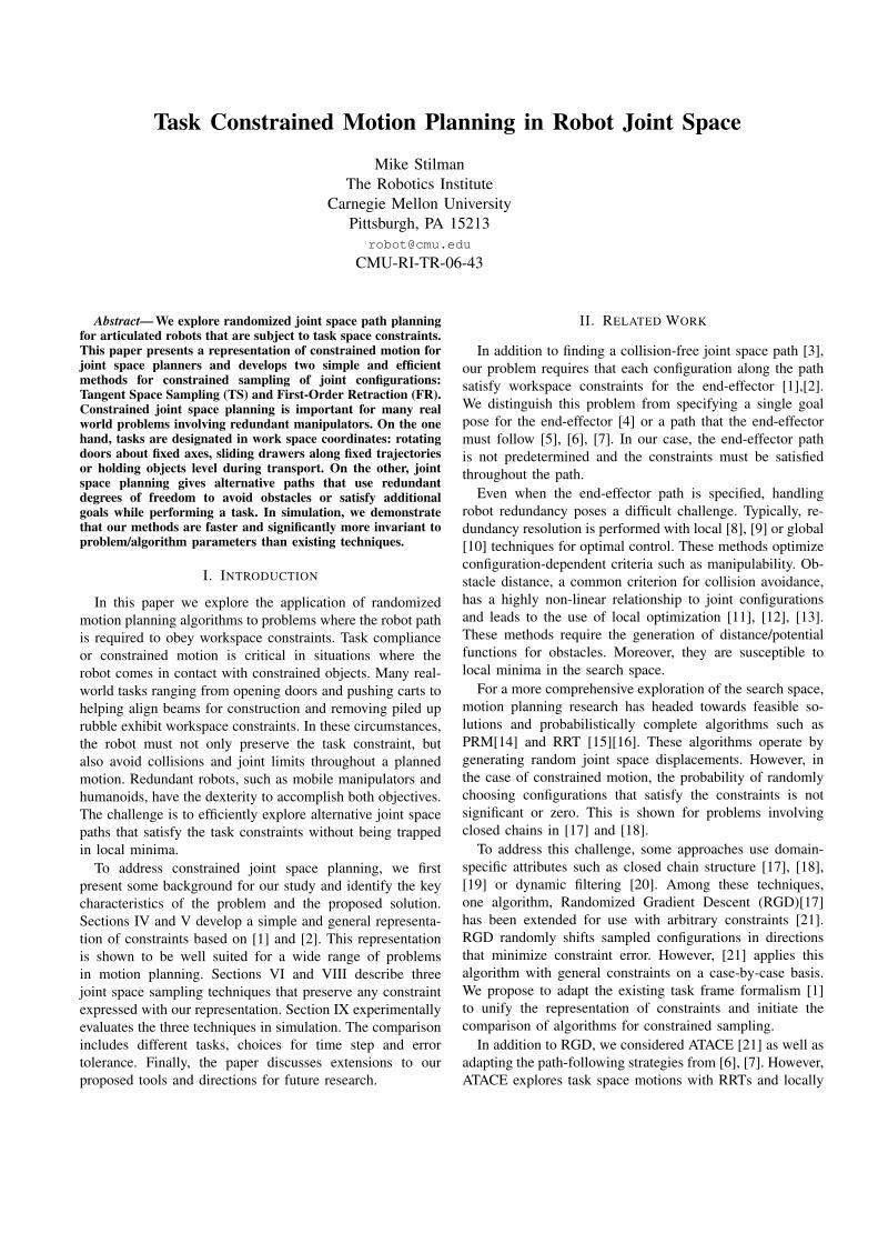
A. Fixed Frames

The simplest task defines a single frame Ft and Ct for theentire path plan. Fixed frame constraints commonly occurwhen manipulating objects that are kinematically linked tothe environment. Figures 6 and 7 show two examples wherelinkages are hinges and rails. F t is chosen as any framein which the axes align with the directions of constrainedmotion. Usually the transformation describing F t, T0

t issimply the position and orientation of the object in theworld frame. Ct indicates which axes of Ft permit validtranslations and rotations.

When planning constrained manipulation, one can assumethat the object is rigidly attached to the robot during grasp.At the time of grasp, let T0

A and T0e represent the position

(a) Fixed C = [ 0 1 1 1 1 1 ]T (b) Fixed C = [ 1 1 1 1 1 0 ]T (c) Para. C = [ 0 0 0 1 1 0 ]T (d) Para. C = [ 1 1 1 1 1 0 ]T

Fig. 1. Examples of constraints implemented with a roll/pitch/yaw specification of task coordinates. The task frames in (c) and (d) areparameterized by the configuration of the robot.

and orientation of object A and the end-effector respectively.We define the grasp transform TG:

TG = TeA = Te

0T0A = (T0

e)−1T0

A (5)

Subsequently, during manipulation, the kinematics of theend-effector are extended to reflect the work space positionof the manipulated object:

T0e′(q) = T0

e(q)TG (6)

With this kinematic extension, C directly specifies the per-mitted displacements of the end-effector frame with respectto the task frame.

B. Simple Frame ParametersSection V-A described a global constraint on the robot

end-effector. Suppose the constraint is defined locally withrespect to the position of the end-effector or another functionof the planner state. Section V-D addresses complex contin-uous definitions of constraints. However, for common tasksa simple parametrization of the task frame is sufficient.

For instance, a task may consist of manipulating a se-quence of constrained objects. Each object is assigned adistinct task frame and constraint vector. The path plannerselects the task frame based on the object or subspace withwhich it is in contact.

Alternatively, the constraint for a single object may bedefined locally with respect to the configuration of the robot.For example, a local constraint on rotation is meaningful fortransporting open containers of liquid such as paint (Fig-ure 8). In this case, the task frame orientation is designatedby the world frame and the position is determined by theend-effector configuration. The constraint vector remains aspecification of the directions of permissible motion.

C. Kinematic Closure ConstraintsAn important constraint for multi-arm manipulation and

reconfigurable robots is a linkage with a closed kinematicchain. One approach to specifying kinematic closure is tobreak the chain at an arbitrary joint jk. The linkage becomesan open chain with a constraint defined by the freedoms ofthe detached joint jk.

We formulate closure as a special case of parameterizedtask frame constraints. For any open chain joint configura-tion, q, the kinematic expression for jk along each chain

yields a work space transform T(q) describing jk withrespect to F0. One of these transforms can be specified as thetask frame, T0

t (q) while the others are end-effectors T0e(q).

As with previous examples, the constraint vector intuitivelyspecifies the degrees of freedom for the joint jk.

D. Constraint Paths and Surfaces

Some elaborate constraints may require the end-effectorto remain on a non-linear path or maintain contact with acomplex surface. In this case there are at least three options:

1) Parameterize the task frame by the nearest position onthe path or surface to the sampled configuration.

2) Parameterize the surface by a subset of standardorthogonal coordinates and constrain the remainingcoordinates to the surface values.

3) Define a coordinate system that implicitly encodes dis-tance from the surface as a change to the coordinates.

The first option may require global or local optimizationto determine the nearest surface point. The second avoidsthis computation by deciding the values for the parametercoordinates as a function of the sampled configuration.However, this approach may not always be possible andit would also lead to an asymmetric exploration of theconstraint manifold. The final alternative could prove difficultto represent globally, yet it may be implemented locally withnumerical regression techniques [22].

Notice that in the case where a path is parameterized bytime, the end-effector trajectory is a continuous sequence oftask frame parameters. Extending the search space with time,the frame of a sampled configuration is decided by time.

VI. INTRODUCING CONSTRAINED SAMPLING

In selecting a representation of task constraints we iden-tified a linear subspace of constrained configurations forthe end-effector in the task space. This is the space of allcoordinates x in F t such that xi = 0 when ci = 1. This spacemay map to a non-linear manifold in robot joint space. Whensampling the joint space, randomized planners will typicallyproduce samples that lie outside the constraint manifold.Our proposed methods use C to formulate a distance metricin task space and either select or project samples within atolerance distance (ε) of the constraint manifold.

A. Computing Distance

Having identified a sampled configuration qs, we computethe forward kinematics for qs. Commonly the end-effectorframe, Fe, is found in homogeneous coordinates as thetransformation T0

e(qs). The displacement of Fe with respectto the task frame F t is found by:

Tte(qs) = Tt

0T0e(qs) = (T0

t )−1T0

e(qs) (7)

We now represent the transform for end-effector displace-ment with respect to the task frame in task coordinates.The Appendix also defines this change in representation forroll/pitch/yaw.

∆x ≡ Tte(qs) (8)

The task space error is found simply by the product in Eq. 9.This product has the effect of selection presented in Eq. 10.

∆xerr =[e1 . . . en

]= C∆x (9)

ei ={

0 ci = 0∆xi ci = 1 (10)

B. Baseline: Randomized Gradient Descent

The proposed distance metric detects when a configurationsatisfies the constraint tolerance. Furthermore, it can be usedto identify task space motions that reduce error. Our algo-rithms use this information to construct constrained samples.

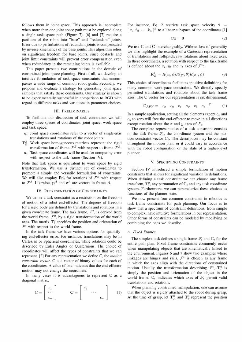
The three methods we compare are Randomized GradientDescent (RGD) [17][21], Tangent-Space Sapmling (TS), andFirst-Order Retraction (FR). For simplicity, we will describeeach approach as a modification to the basic RRT algorithmsummarized in Figure 2. The algorithm samples a randomconfiguration qrand and finds its nearest neighbor in the treeqnear. The sampled configuration qs is placed at a fixeddistance ∆t along the vector from qnear to qrand.

As a baseline, let us consider the RGD algorithm detailedin Figure 3. After computing the task space error of qs, thismethod continues to uniformly sample the neighborhood ofthe configuration within a radius dmax. The error of eachnew configuration q′s is evaluated and compared with qs.If the error is less, q′s is substituted for qs. The procedureterminates when the error is less than ε or the maximumiteration count is met.

VII. RELATING JOINT MOTION TO CONSTRAINT ERROR

Due to random selection, the RGD algorithm will typ-ically evaluate forward kinematics for a large number ofconfigurations that result in greater task space error. Theseconfigurations are discarded. To avoid this computation, wepropose to identify the relationship between task space errorand joint space motion. Since this relationship is nonlinear,we use a first-order approximation.

The basic Jacobian, J0, is a matrix of partial derivativesrelating joint space velocities to end-effector linear andangular velocities. We will compute Jt, the Jacobian for thetask frame. The Jacobian inverse will perform the inversemapping, allowing us to identify joint space displacementsthat resolve task space error.

TASK CONSTRAINED RRT(qinit,∆t)1 T .init(qinit);2 for a = 1 to A3 do qrand ← RANDOM CONFIG;4 qnear ← NEAREST NEIGHBOR(qrand, T );5 qdir ← (qrand − qnear)/|qrand − qnear|;6 qs = qnear + qdir ∆t;7 if *CONSTRAINED* NEW CONFIG(qs,qnear)8 then T . add vertex (qs);9 T . add edge (qnear,qs);

10 return T

COMPUTE TASK ERROR(qs,qnear)1 (C,Tt

0)← RETRIEVE CONSTRAINT(qs,qnear);2 T0

e ← FORWARD KINEMATICS(qs);3 Tt

e ← Tt0T

0e;

4 ∆x← TASK COORDINATES(Tte);

5 ∆xerr ← C∆x6 return ∆xerr;

Fig. 2. Pseudo-code for the Task-Constrained RRT (TC-RRT) constructionalgorithm. The word *CONSTRAINED* represents either RGD, TS or FR.COMPUTE TASK ERROR is common among all three subroutines.

A. Task Frame Jacobian

The Jacobian of a robot manipulator, J0, can be computedanalytically given the kinematics of each joint at a sampledconfiguration qs of the robot. [23] For end-effector positionp0, joint positions p0

i and oriented joint axes z0i , we have:

J0 =[JP1 . . . JPnJO1 . . . JOn

](11)

[JPiJOi

]=

[

zi−1

0

](prismatic joint)[

zi−1 × (p− pi−1)zi−1

](revolute joint)

(12)

Typically, this computation is performed in the world frameF0. We invert the orientation of the task frame, R0

t , andtransform the Jacobian into F t as follows:

Jt =[

Rt0 0

0 Rt0

]J0 (13)

The lower three rows of J0 and Jt map to angular velocities.However, angular velocities are not instantaneous changes toany actual parameters that can be used to represent orien-tation. Given the configuration qs, instantaneous velocitieshave a linear relationship E(qs) to the time derivatives ofmany position and orientation parameters.[2]

J(qs) = E(qs)Jt(qs) (14)

The matrix E(q) is presented in the Appendix for Cartesiantranslations and RPY rotations.

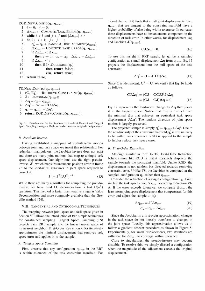
RGD NEW CONFIG(qs,qnear)1 i← 0; j ← 0;2 ∆xerr ← COMPUTE TASK ERROR(qs,qnear);3 while i < I and j < J and |∆xerr| > ε4 do i← i+ 1; j ← j + 1;5 q′s = qs + RANDOM DISPLACEMENT(dmax);6 ∆x′err ← COMPUTE TASK ERROR(qs,qnear);7 if ∆x′err < ∆xerr8 then j ← 0; qs = q′s; ∆xerr = ∆x′err;9 if ∆xerr ≤ ε

10 then if IN COLLISION(qs)11 then return false;12 else return true;13 return false;

TS NEW CONFIG(qs,qnear)1 (C,Tt

0)← RETRIEVE CONSTRAINT(qs,qnear);2 J← JACOBIAN(qnear);3 ∆q = qs − qnear;4 ∆q′ = ∆q− J†CJ∆q;5 qs ← qnear + ∆q′;6 return RGD NEW CONFIG(qs,qnear);

Fig. 3. Pseudo-code for the Randomized Gradient Descent and TangentSpace Sampling strategies. Both methods constrain sampled configurations.

B. Jacobian Inverse

Having established a mapping of instantaneous motionbetween joint and task space we invert this relationship. Forredundant manipulators, the Jacobian inverse does not existand there are many joint motions that map to a single taskspace displacement. Our algorithms use the right pseudo-inverse, J†, which maps instantaneous position error in frameF t to the least-norm velocities in joint space required tocorrect it.

J† = JT (JJT )−1 (15)

While there are many algorithms for computing the pseudo-inverse, we have used LU decomposition, a fast O(n3)operation. This method is faster than iterative Singular ValueDecomposition and more commonly available than the Gre-ville method [24].

VIII. TANGENTIAL AND ORTHOGONAL TECHNIQUES

The mapping between joint space and task space given inSection VII allows the introduction of two simple techniquesfor constrained sampling. Tangent Space Sampling (TS)projects each RRT sample into the linear tangent space ofits nearest neighbor. First-Order Retraction (FR) iterativelyapproximates the minimal displacement that removes taskspace error and applies it to the sample.

A. Tangent Space Sampling

First, observe that any configuration qnear in the RRTis within tolerance of the task constraint manifold. For

closed chains, [25] finds that small joint displacements fromqnear that are tangent to the constraint manifold have ahigher probability of also being within tolerance. In our case,these displacements have no instantaneous component in thedirection of task error. In other words, for displacement ∆qand Jacobian J(qnear),

CJ∆q = 0. (16)

To use this insight in RRT search, let qs be a sampledconfiguration at a small displacement ∆q from qnear. Eq. 17projects the displacement into the null space of the taskconstraint.

∆q′ = (I− J†CJ)∆q (17)

Since C is idempotent, C2 = C. We verify that Eq. 16 holdsas follows:

CJ∆q′ = (CJ−CCJJ†J)∆q

= (CJ−CJ)∆q = 0 (18)

Eq. 17 represents the least-norm change to ∆q that placesit in the tangent space. Notice that this is distinct fromthe minimal ∆q that achieves an equivalent task spacedisplacement J∆q′. The random direction of joint spacemotion is largely preserved.

The projected sample is simply q′s = qnear+∆q′. Due tothe non-linearity of the constraint manifold,q′s is still unlikelyto be within error tolerance. RGD is applied to the sampleto further reduce task space error.

B. First-Order Retraction

Although similar in form to TS, First-Order Retractionbehaves more like RGD in that it iteratively displaces thesample towards the constraint manifold. Unlike RGD, thedisplacement is not random but directed towards removingconstraint error. Unlike TS, the Jacobian is computed at thesampled configuration qs rather than qnear.

Consider the retraction of a single configuration qs. First,we find the task space error, ∆xerr, according to Section VI-A. If the error exceeds tolerance, we compute ∆qerr, theleast-norm joint space displacement that compensates for thiserror and adjust the sample to q′s:

∆qerr = J†∆xerr (19)q′s = qs −∆qerr (20)

Since the Jacobian is a first-order approximation, changesin the task space do not linearly transform to changes inthe joint space. Locally, this approximation allows us tofollow a gradient descent procedure as shown in Figure 5.Experimentally, for small displacements, two iterations aresufficient for ∆xerr to converge within tolerance.

Close to singularities, the pseudo-inverse may becomeunstable. To resolve this, we simply discard a configurationwhen the magnitude of the adjustment exceeds the originaldisplacement.

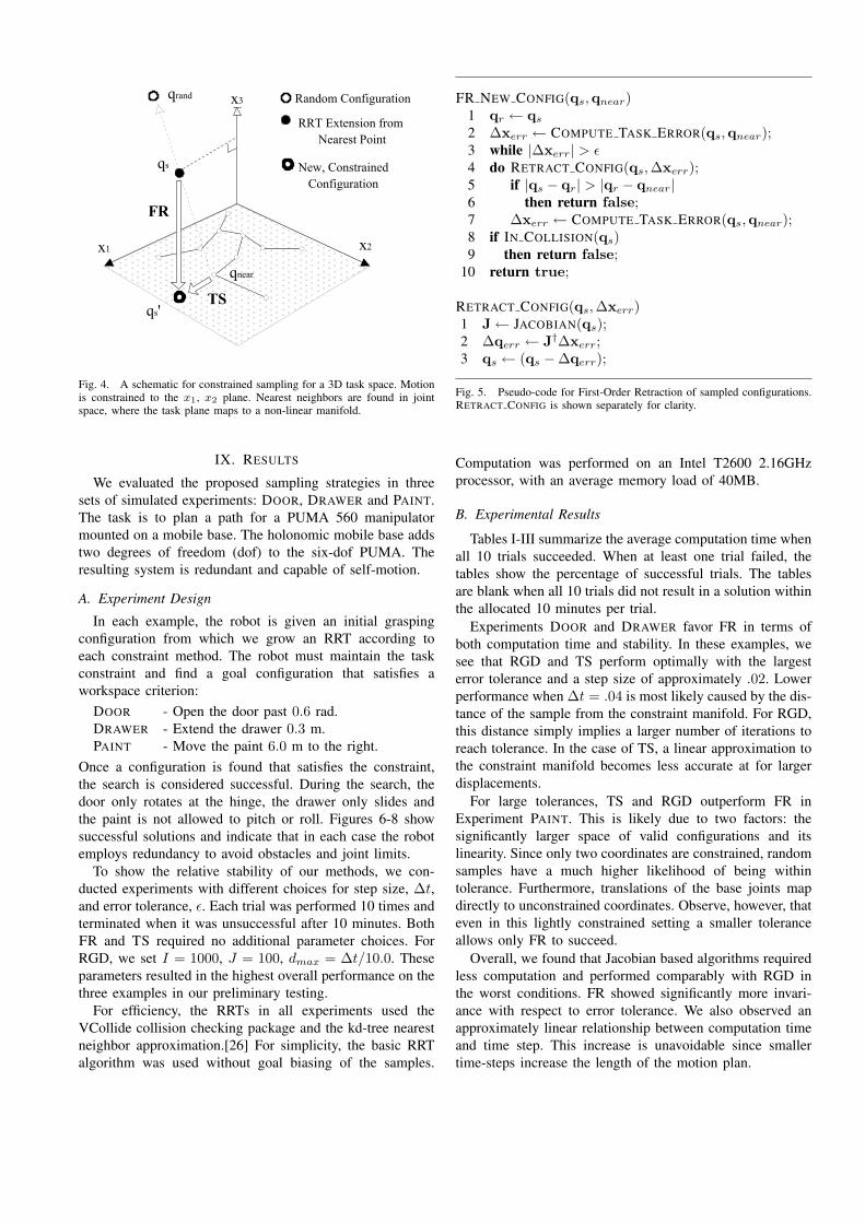
Fig. 4. A schematic for constrained sampling for a 3D task space. Motionis constrained to the x1, x2 plane. Nearest neighbors are found in jointspace, where the task plane maps to a non-linear manifold.

IX. RESULTS

We evaluated the proposed sampling strategies in threesets of simulated experiments: DOOR, DRAWER and PAINT.The task is to plan a path for a PUMA 560 manipulatormounted on a mobile base. The holonomic mobile base addstwo degrees of freedom (dof) to the six-dof PUMA. Theresulting system is redundant and capable of self-motion.

A. Experiment Design

In each example, the robot is given an initial graspingconfiguration from which we grow an RRT according toeach constraint method. The robot must maintain the taskconstraint and find a goal configuration that satisfies aworkspace criterion:

DOOR - Open the door past 0.6 rad.DRAWER - Extend the drawer 0.3 m.PAINT - Move the paint 6.0 m to the right.

Once a configuration is found that satisfies the constraint,the search is considered successful. During the search, thedoor only rotates at the hinge, the drawer only slides andthe paint is not allowed to pitch or roll. Figures 6-8 showsuccessful solutions and indicate that in each case the robotemploys redundancy to avoid obstacles and joint limits.

To show the relative stability of our methods, we con-ducted experiments with different choices for step size, ∆t,and error tolerance, ε. Each trial was performed 10 times andterminated when it was unsuccessful after 10 minutes. BothFR and TS required no additional parameter choices. ForRGD, we set I = 1000, J = 100, dmax = ∆t/10.0. Theseparameters resulted in the highest overall performance on thethree examples in our preliminary testing.

For efficiency, the RRTs in all experiments used theVCollide collision checking package and the kd-tree nearestneighbor approximation.[26] For simplicity, the basic RRTalgorithm was used without goal biasing of the samples.

FR NEW CONFIG(qs,qnear)1 qr ← qs2 ∆xerr ← COMPUTE TASK ERROR(qs,qnear);3 while |∆xerr| > ε4 do RETRACT CONFIG(qs,∆xerr);5 if |qs − qr| > |qr − qnear|6 then return false;7 ∆xerr ← COMPUTE TASK ERROR(qs,qnear);8 if IN COLLISION(qs)9 then return false;

10 return true;

RETRACT CONFIG(qs,∆xerr)1 J← JACOBIAN(qs);2 ∆qerr ← J†∆xerr;3 qs ← (qs −∆qerr);

Fig. 5. Pseudo-code for First-Order Retraction of sampled configurations.RETRACT CONFIG is shown separately for clarity.

Computation was performed on an Intel T2600 2.16GHzprocessor, with an average memory load of 40MB.

B. Experimental Results

Tables I-III summarize the average computation time whenall 10 trials succeeded. When at least one trial failed, thetables show the percentage of successful trials. The tablesare blank when all 10 trials did not result in a solution withinthe allocated 10 minutes per trial.

Experiments DOOR and DRAWER favor FR in terms ofboth computation time and stability. In these examples, wesee that RGD and TS perform optimally with the largesterror tolerance and a step size of approximately .02. Lowerperformance when ∆t = .04 is most likely caused by the dis-tance of the sample from the constraint manifold. For RGD,this distance simply implies a larger number of iterations toreach tolerance. In the case of TS, a linear approximation tothe constraint manifold becomes less accurate at for largerdisplacements.

For large tolerances, TS and RGD outperform FR inExperiment PAINT. This is likely due to two factors: thesignificantly larger space of valid configurations and itslinearity. Since only two coordinates are constrained, randomsamples have a much higher likelihood of being withintolerance. Furthermore, translations of the base joints mapdirectly to unconstrained coordinates. Observe, however, thateven in this lightly constrained setting a smaller toleranceallows only FR to succeed.

Overall, we found that Jacobian based algorithms requiredless computation and performed comparably with RGD inthe worst conditions. FR showed significantly more invari-ance with respect to error tolerance. We also observed anapproximately linear relationship between computation timeand time step. This increase is unavoidable since smallertime-steps increase the length of the motion plan.

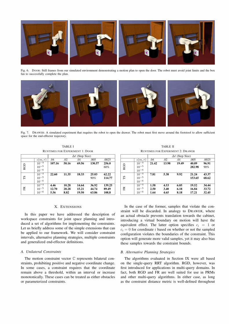
Fig. 6. DOOR: Still frames from our simulated environment demonstrating a motion plan to open the door. The robot must avoid joint limits and the boxfan to successfully complete the plan.

Fig. 7. DRAWER: A simulated experiment that requires the robot to open the drawer. The robot must first move around the footstool to allow sufficientspace for the end-effector trajectory.

TABLE IRUNTIMES FOR EXPERIMENT 1: DOOR

∆t (Step Size)ε(m, r) .04 .02 .01 .005 .0025

RG

D 10−4 107.16 50.16 69.56 130.57 256.010−5 60%10−6

TS

10−4 22.60 11.35 18.33 25.03 62.2210−5 90% 114.7710−6

FR

10−4 4.46 10.28 14.64 36.92 139.2510−5 12.70 20.28 15.21 44.74 89.4910−6 5.56 8.82 19.50 63.86 108.8

X. EXTENSIONS

In this paper we have addressed the description ofworkspace constraints for joint space planning and intro-duced a set of algorithms for implementing the constraints.Let us briefly address some of the simple extensions that canbe applied to our framework. We will consider constraintintervals, alternative planning strategies, multiple constraintsand generalized end-effector definitions.

A. Unilateral Constraints

The motion constraint vector C represents bilateral con-straints, prohibiting positive and negative coordinate change.In some cases, a constraint requires that the coordinateremain above a threshold, within an interval or increasemonotonically. These cases can be treated as either obstaclesor parameterized constraints.

TABLE IIRUNTIMES FOR EXPERIMENT 2: DRAWER

∆t (Step Size)ε(m, r) .04 .02 .01 .005 .0025

RG

D 10−4 21.42 13.98 19.49 40.09 96.9110−5 282.98 90%10−6

TS

10−4 7.81 5.38 9.92 21.24 43.3710−5 153.65 68.6210−6

FR

10−4 1.58 4.53 6.05 19.52 34.4410−5 2.50 3.40 6.18 16.84 33.7210−6 1.64 4.65 8.18 17.21 32.45

In the case of the former, samples that violate the con-straint will be discarded. In analogy to DRAWER, wherean actual obstacle prevents translation towards the cabinet,introducing a virtual boundary on motion will have theequivalent effect. The latter option specifies ci = 1 orci = 0 for coordinate i based on whether or not the sampledconfiguration violates the boundaries of the constraint. Thisoption will generate more valid samples, yet it may also biasthese samples towards the constraint bounds.

B. Alternative Planning Strategies

The algorithms evaluated in Section IX were all basedon the single-query RRT algorithm. RGD, however, wasfirst introduced for applications in multi-query domains. Infact, both RGD and FR are well suited for use in PRMsand other multi-query algorithms. In either case, as longas the constraint distance metric is well-defined throughout

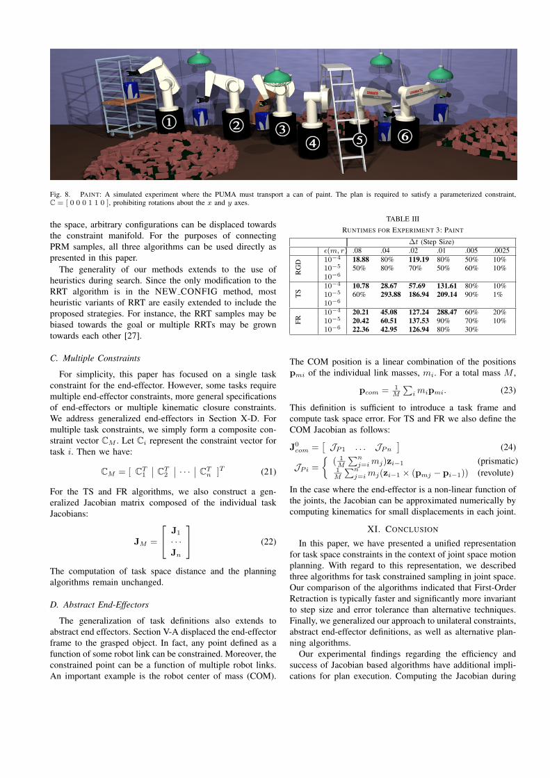
Fig. 8. PAINT: A simulated experiment where the PUMA must transport a can of paint. The plan is required to satisfy a parameterized constraint,C = [ 0 0 0 1 1 0 ], prohibiting rotations about the x and y axes.

the space, arbitrary configurations can be displaced towardsthe constraint manifold. For the purposes of connectingPRM samples, all three algorithms can be used directly aspresented in this paper.

The generality of our methods extends to the use ofheuristics during search. Since the only modification to theRRT algorithm is in the NEW CONFIG method, mostheuristic variants of RRT are easily extended to include theproposed strategies. For instance, the RRT samples may bebiased towards the goal or multiple RRTs may be growntowards each other [27].

C. Multiple Constraints

For simplicity, this paper has focused on a single taskconstraint for the end-effector. However, some tasks requiremultiple end-effector constraints, more general specificationsof end-effectors or multiple kinematic closure constraints.We address generalized end-effectors in Section X-D. Formultiple task constraints, we simply form a composite con-straint vector CM . Let Ci represent the constraint vector fortask i. Then we have:

CM = [ CT1 CT2 · · · CTn ]T (21)

For the TS and FR algorithms, we also construct a gen-eralized Jacobian matrix composed of the individual taskJacobians:

JM =

J1

· · ·Jn

(22)

The computation of task space distance and the planningalgorithms remain unchanged.

D. Abstract End-Effectors

The generalization of task definitions also extends toabstract end effectors. Section V-A displaced the end-effectorframe to the grasped object. In fact, any point defined as afunction of some robot link can be constrained. Moreover, theconstrained point can be a function of multiple robot links.An important example is the robot center of mass (COM).

TABLE IIIRUNTIMES FOR EXPERIMENT 3: PAINT

∆t (Step Size)ε(m, r) .08 .04 .02 .01 .005 .0025

RG

D 10−4 18.88 80% 119.19 80% 50% 10%10−5 50% 80% 70% 50% 60% 10%10−6

TS

10−4 10.78 28.67 57.69 131.61 80% 10%10−5 60% 293.88 186.94 209.14 90% 1%10−6

FR

10−4 20.21 45.08 127.24 288.47 60% 20%10−5 20.42 60.51 137.53 90% 70% 10%10−6 22.36 42.95 126.94 80% 30%

The COM position is a linear combination of the positionspmi of the individual link masses, mi. For a total mass M ,

pcom = 1M

∑imipmi. (23)

This definition is sufficient to introduce a task frame andcompute task space error. For TS and FR we also define theCOM Jacobian as follows:

J0com =

[JP1 . . . JPn

](24)

JPi ={

( 1M

∑nj=imj)zi−1 (prismatic)

1M

∑nj=imj(zi−1 × (pmj − pi−1)) (revolute)

In the case where the end-effector is a non-linear function ofthe joints, the Jacobian can be approximated numerically bycomputing kinematics for small displacements in each joint.

XI. CONCLUSION

In this paper, we have presented a unified representationfor task space constraints in the context of joint space motionplanning. With regard to this representation, we describedthree algorithms for task constrained sampling in joint space.Our comparison of the algorithms indicated that First-OrderRetraction is typically faster and significantly more invariantto step size and error tolerance than alternative techniques.Finally, we generalized our approach to unilateral constraints,abstract end-effector definitions, as well as alternative plan-ning algorithms.

Our experimental findings regarding the efficiency andsuccess of Jacobian based algorithms have additional impli-cations for plan execution. Computing the Jacobian during

planning allows us to measure the manipulability of sam-pled configurations: det(JJT )1/2 [28]. Due to online errors,successful execution may require compliance or impedancecontrol. Maintaining a manipulability threshold will ensurerobot stability when it deviates from the motion plan.

Many facets of task constrained planning remain for futureinvestigation. Each of the extensions in Section X can beexplored. For instance, Section X-C applies our method withmultiple hard constraints. A study of soft constraints maylead to results in biasing motion plans towards desirablerobot postures. In these cases, task projection into the nullspace of J† could be used to prioritize constraints.[29], [30]

Of course, soft constraints are one of many possibledeeper explorations of constrained search. We introducesuch examples to show the modularity and accessibility ofthe methods described in this paper. Our proposed toolsdemonstrate the feasibility of task constrained joint spaceplanning and provide a groundwork for further research.

XII. ACKNOWLEDGEMENTS

We are grateful to James Kuffner, Jaeheung Park andChris Atkeson for their comments and advice throughout thedevelopment of this work. We thank Jan-Ullrich Schamburekfor his contributions to the experimental environment thatinspired and enabled this research.

APPENDIX

The examples in this paper, as well as many commonconstraints, can be expressed with a C vector in a coordinatesystem composed of Cartesian translation and fixed axis(roll/pitch/yaw) rotation. The use of any coordinate systemrequires us to derive translations of displacements.

For reference, we give the transformation from error inhomogeneous coordinates to fixed axis coordinates. We alsoshow the E(q) matrix for the fixed axis representation.Similar methods can be applied to other coordinate systems.

Since forward kinematics are typically expressed in termsof homogeneous transformations, Eq. 25 gives the mappingfrom a transformation matrix to Cartesian / fixed axis co-ordinates. The Cartesian component is equivalent to the lastcolumn of the transformation. For Ta,b representing the valueat row a, column b of T :

ψ = atan2(T3,2, T3,3)θ = −asin(T3,1)φ = atan2(T2,1, T1,1) (25)

In order to apply TS or FR, we also need to map velocities inworkspace to velocities in task space. The angular velocityvector ω is found by a summation of fixed axis velocities ina common frame:

ω =

00φ

+Rz(φ)

0θ0

+Rz(φ)Ry(θ)

ψ00

(26)

This relationship is rearranged as a single matrix, E−1ω (q):

ω = E−1ω (q)

[ψ θ φ

]T(27)

Inverting E−1ω (q) we find Eω(q), a matrix that maps angular

velocities to fixed axis velocities. Adjoining the identitymatrix for linear velocities Eq. 28 specifies E(q).

Erpy(q) =

I3×3 · · · 0 · · ·

... cφ/cθ sφ/cθ 00 −sφ cφ 0... cφsθ/cθ sφsθ/cθ 1

(28)

REFERENCES

[1] M. T. Mason. Compliance and force control for computer controlledmanipulators. IEEE Trans. on Systems, Man, and Cybernetics,, 11(6),1981.

[2] O. Khatib. A unified approach for motion and force control ofrobot manipulators: The operational space formulation. InternationalJournal of Robotics Research, 3(1), 1987.

[3] J.C. Latombe. Robot Motion Planning. Kluwer Academic Publishers,1991.

[4] J. Ahuactzin and K. Gupta. The kinematic roadmap: A motionplanning based global approach for inverse kinematics of redundantrobots. IEEE Trans. on Robotics and Automation, 15:653–669, 1999.

[5] Z. Guo and T. Hsia. Joint trajectory generation for redundant robotsin an environment with obstacles. In IEEE Int. Conf. on Robotics andAutomation, pages 157–162, 1990.

[6] G. Oriolo, M. Ottavi, and M. Vendittelli. Probabilistic motion planningfor redundant robots along given end-effector paths. In IEEE/RSJ Int’lConf. on Intelligent Robots and Systems, 2002.

[7] G. Oriolo and C. Mongillo. Motion planning for mobile manipulatorsalong given end-effector paths. In IEEE Int’l Conf. on Robotics andAutomation (ICRA’05), 2005.

[8] D. P. Martin, J. Baillieul, and J. M. Hollerbach. Resolution ofkienmatic redundancy using opetimization techniques. IEEE Trans.on Robotics and Automation, 5(4):529–533, 1989.

[9] B. Siciliano. Kinematic control of redundant robot manipulators: Atutorial. Journal of Intelligent and Robotic Systems, 3:201–212, 1990.

[10] S. Seereeram and J. T. Wen. A global approach to path planning forredundant manipulators. IEEE Trans. on Robotics and Automation,11(1), 1995.

[11] A. McLean and S. Cameron. The virtual springs method: Path planningand collision avoidance for redundant manipulators. 15, 1996.

[12] Oliver Brock, Oussama Khatib, and Sriram Viji. Task-consistentobstacle avoidance and motion behavior for mobile manipulation. InIEEE Int’l Conf. on Robotics and Automation, 2002.

[13] O. Khatib, L. Sentis, J. Park, and J. Warren. Whole body dynamicbehavior and control of human-like robots. International Journal ofHumanoid Robotics, pages 29–44, 2004.

[14] L. Kavraki, P. Svestka, J. C. Latombe, and M. H. Overmars. Prob-abilistic roadmaps for path planning high-dimensional configurationspaces. IEEE Trans. on Robotics and Automation, 12(4), 1996.

[15] S.M.LaValle. Rapidly-exploring random trees: A new tool for pathplanning. Technical report, Computer Science Dept., Iowa StateUniversity, 1998.

[16] S.M. LaValle and J.J. Kuffner. Rapidly exploring random trees:Progress and prospects. In Workshop on the Algorithmic Foundationsof Robotics, 2000.

[17] S. M. LaValle, J. Yakey, and L. E. Kavraki. A probabilistic roadmapapproach for systems with closed kinematic chains. In In Proc. IEEEInt’l Conf. on Robotics and Automation, 1999.

[18] L. Han and N. Amato. A kinematics-based probabilistic roadmapmethod for closed chain systems. In Workshop on AlgorithmicFoundations of Robotics (WAFR), 2000.

[19] J. Cortes T. Simeon and J.P. Laumond. A random loop generator forplanning the motions of closed kinematic chains with prm methods.In IEEE Int. Conf. on Robotics and Automation, 2002.

[20] J.J. Kuffner, K. Nishiwaki, S. Kagami, M. Inaba, and H. Inoue.Motion planning for humanoid robots under obstacle and dynamicbalance constraints. In IEEE Int’l Conf. on Robotics and Automation(ICRA’01), pages 692–698, 2001.

[21] Z. Yao and K. Gupta. Path planning with general end-effectorconstraints: Using task space to guide configuration space search. InIEEE/RSJ Int’l Conf. on Intelligent Robots and Systems, 2005.

[22] C. G. Atkeson, A. W. Moore, and S. Schaal. Locally weightedlearning. 11:11–73, 1997.

[23] L. Sciaviccio and B. Siciliano. Modeling and control of robotmanipulators. McGraw-Hill Co., 1996.

[24] T. N. E. Greville. Some applications of the pseudoinverse of a matrix.SIAM Review, 2:15–22, 1960.

[25] J. Yakey, S.M. LaValle, and L. E. Kavraki. Randomized path planningfor linkages with closed kinematic chains. IEEE Transactions onRobotics and Automation, 17(7), 2001.

[26] A. Atramentov and S. M. LaValle. Efficient nearest neighbor searchingfor motion planning. In IEEE Int’l Conf. on Robotics and Automation(ICRA’02), 2002.

[27] J. Kuffner and S. M. LaValle. Rrt-connect: An efficient approachto single-query path planning. In Workshop on the AlgorithmicFoundations of Robotics, pages 995–1001.

[28] T. Yoshikawa. Manipulability of robotic mechanisms. Int. Journal ofRobotics Research, 4:3–9, 1985.

[29] H. Hanafusa, T. Yoshikawa, and Y. Nakamura. Analaysis and controlof articulated robot with redundancy. In IFAC, 8th Triennal WorldCongress, volume 4, pages 1927–1932, 1981.

[30] R. Boulic P. Baerlocher. Task-priority formulations for the kinematiccontrol of highly redundant atriculated structures. In Int. Conf. onIntelligent Robots and Systems, 1998.