Targeted Debt Relief and the Origins of Financial Distress:

Experimental Evidence from Distressed Credit Card Borrowers∗

Will DobbiePrinceton University and NBER

Jae SongSocial Security Administration

May 3, 2017

Abstract

We study the drivers of financial distress using a large-scale field experiment that offeredrandomly selected borrowers a combination of (i) immediate payment reductions to target short-run liquidity constraints and (ii) delayed debt write-downs to target long-run debt constraints.We identify the separate effects of the payment reductions and write-downs using variation fromboth the experiment and cross-sectional differences in treatment intensity. Surprisingly, we findthat the debt write-downs significantly improved both financial and labor market outcomesdespite not taking effect until three to five years after the randomization. In sharp contrast,there were no positive effects of the immediate payment reductions. These results run counterto the widespread view that financial distress is largely the result of short-run constraints.

∗A previous version of this paper was circulated under the title “Debt Relief or Debt Restructuring? Evidencefrom an Experiment with Distressed Credit Card Borrowers.” We are extremely grateful to Ann Woods and RobertKaplan at Money Management International, David Jones at the Association of Independent Consumer CreditCounseling Agencies, Ed Falco at Auriemma Consulting Group, and Gerald Ray and David Foster at the SocialSecurity Administration for their help and support. We thank Tal Gross, Matthew Notowidigdo, and Jialan Wangfor providing the bankruptcy data used in this analysis. We also thank Leah Platt Boustan, Hank Farber, JamesFeigenbaum, Paul Goldsmith-Pinkham, Tal Gross, Larry Katz, Ben Keys, Patrick Kline, Ilyana Kuziemko, AlexMas, Jesse Shapiro, Andrei Shleifer, Crystal Yang, Jonathan Zinman, Eric Zwick, and numerous seminar participantsfor helpful comments and suggestions. Kevin DeLuca, Daniel Herbst, Disa Hynsjo, Samsun Knight, Kevin Tang,Daniel Van Deusen, Amy Wickett, and Yining Zhu provided excellent research assistance. Financial support fromthe Washington Center for Equitable Growth is gratefully acknowledged. Correspondence can be addressed to theauthors by e-mail: wdobbie@princeton.edu [Dobbie] or jae.song@ssa.gov [Song]. Any opinions expressed herein arethose of the authors and not those of the Social Security Administration.

Financial distress is extraordinarily common in the United States. Over one-third of Americans

have a debt in collections, and more than one in ten will file for bankruptcy at some point during

their lives. Americans are also severely liquidity constrained, with approximately one-quarter of

households unable to come up with $2,000 to cope with an unexpected need (Lusardi, Schneiderm,

and Tufano 2011).1 As a result, there is a widespread view that liquidity constraints are the most

important driver of financial distress, and that debt relief will be most effective if it is designed

to alleviate these kinds of short-run constraints. This view has important implications for under-

standing both the growing levels of financial distress in the United States and the optimal design

of debt relief programs such as consumer bankruptcy. In this paper, however, we show that this

view significantly overstates the benefits of debt relief targeting short-run liquidity constraints,

while significantly understating the benefits of targeting longer-run financial constraints such as

the distortionary effects of excessive debt (so called “debt overhang”).

Estimating the effects of targeted debt relief is challenging because most debt relief programs

are designed to address both short- and long-run financial constraints at the same time. For

example, consumer bankruptcy protection offers both lower minimum payments (to address short-

run liquidity constraints) and generous debt write-downs (to address longer-run debt overhang

constraints). As a result, standard “black box” estimates cannot be used to predict the effects of

specific types of debt relief or to understand the relative importance of addressing either short-

or long-run financial constraints alone. An added complication is that the recipients of most debt

relief programs are negatively selected, biasing cross-sectional comparisons, and many of the most

proximate causes of debt relief take-up such as job loss and expense shocks also impact later

outcomes, biasing within-individual comparisons.

In this paper, we estimate the causal impact of targeted debt relief using information from a

randomized field experiment matched to administrative tax, bankruptcy, and credit records. The

experiment was designed and implemented by a large non-profit credit counseling organization in

the context of an important but under-studied debt relief program called the Debt Management

Plan (DMP). The DMP is a structured repayment program that allows distressed borrowers to

simultaneously repay all of their outstanding credit card debt over a three to five year period. In

exchange for enrolling in the repayment program, credit card issuers will usually lower the minimum

payment amount (to address short-run liquidity constraints) and provide a partial write-down of

1An additional 19 percent of households could only come up with $2,000 by pawning or selling possessions ortaking out a payday loan (Lusardi, Schneider, and Tufano 2011). There is also evidence that many households havea high marginal propensity to consume out of both transitory income shocks (e.g., Johnson, Parker, and Souleles2006, Parker et al. 2013) and new liquidity (e.g., Gross and Souleles 2002, Agarwal, Souleles, and Liu 2007, Agarwalet al. 2015, Gross, Notowidigdo, and Wang 2016), and recent work shows large changes in financial distress andconsumption just after anticipated reductions in mortgage interest rates (e.g., Di Maggio, Kermani, and Ramcharan2014, Keys et al. 2014, Fuster and Willen 2015). There is also an important literature showing that present-biasedpreferences can potentially explain both low levels of liquidity and the use of high-cost credit (e.g., Laibson 1997,Heidhues and Koszegi 2010, Meier and Sprenger 2010, Laibson et al. 2017). See DellaVigna (2009) and Zinman(2015) for reviews of the literature on present-biased preferences and liquidity constraints, respectively. Evidence onlonger-run problems such as debt overhang is more limited, although recent work shows that debt overhang can affecta household’s labor supply (Bernstein 2016), entrepreneurial activity (Adelino, Schoar, and Severino 2013), and homeinvestment (Melzer forthcoming).

1

interest payments and late fees (to address longer-run debt overhang). With more than 600,000

individuals enrolling in these repayment programs each year, the DMP is one of the most important

alternatives to consumer bankruptcy in the United States (Wilshusen 2011).

During the experiment, borrowers in both the treatment and control groups were offered a repay-

ment program. However, while control borrowers were offered the status quo repayment program

that had been offered to all borrowers prior to the randomized trial, treated borrowers were offered

a much more generous repayment program that included a combination of two different types of

targeted debt relief: (i) immediate minimum payment reductions meant to address short-run liquid-

ity constraints and (ii) delayed debt write-downs meant to address longer-run debt overhang. The

additional debt relief provided by the experiment was substantial: the typical minimum payment

reduction was just over $26 (a 6.15 percent change from the status quo program), while the typical

debt write-down was $1,712 (a 49.17 percent change from the status quo program). The economic

magnitudes of the payment reductions and debt write-downs were also relatively similar, at least

as measured by the net present costs to the lender (approximately $440 for the typical borrower).

An important feature of the experiment is the tremendous cross-sectional variation in potential

treatment intensity. Each of the credit card issuers participating in the randomized trial offered a

different combination of debt write-downs and minimum payment reductions to treated borrowers,

and individual borrowers made different decisions about how much to borrow from each of these

credit card issuers before the experiment began. These decisions translated into economically

significant differences in the debt write-downs and minimum payment reductions offered to the

treatment group. For example, moving from the 25th percentile to the 75th percentile of debt

write-downs within the treatment group is roughly equivalent to moving from the treatment group

to the control group at the median (a $1,521 change versus a $1,712 change). Similarly, moving

from the 25th to the 75th percentile of minimum payment reductions within the treatment group is

slightly larger than moving from treatment group to the control group at the median (a $33 change

versus a $26 change).

We identify the separate impact of the debt write-downs and minimum payment reductions using

variation from both the randomized experiment and these cross-sectional differences in treatment

intensity. To see the intuition for our approach, imagine a group of borrowers with a low debt

write-down intensity and a low minimum payment intensity, and a second group of borrowers

with a high debt write-down intensity but the same low minimum payment intensity. In this

scenario, we can isolate the impact of a larger debt write-down at the margin by comparing the

effect of treatment eligibility for the low debt write-down intensity borrowers to the effects of

treatment eligibility for the high write-down intensity borrowers. We can similarly isolate the

causal impact of the minimum payment reductions at the margin by comparing the effects of

treatment eligibility for borrowers with different minimum payment intensities but identical debt

write-down intensities. Our approach builds on identification strategies commonly used in studies

of local labor markets, immigration, and trade, which exploits the combination of state- or city-

level variation in potential treatment intensity and national-level variation in treatment status (e.g.,

2

Bartik 1991, Blanchard and Katz 1992, Card 2001, Autor, Dorn, and Hanson 2013). In contrast to

these earlier studies, however, we use individual-level differences in treatment status determined by

random assignment and individual-level differences in potential treatment intensity determined by

decisions made without knowledge of the experiment. As a result, our research design is robust to

many of the potential concerns that typically arise from these types of instruments (e.g., Goldsmith-

Pinkham, Sorkin, and Swift 2017). Using this approach, we measure the effects of the experiment

on repayment, bankruptcy, collections debt, credit scores, employment, and savings using four

administrative datasets matched for the purposes of this study.

We begin by estimating intent-to-treat effects that measure the impact of both the debt write-

downs and minimum payment reductions. We find that treatment eligibility increased the prob-

ability of finishing the repayment program and decreased the probability of filing for bankruptcy,

particularly for borrowers with the highest debt-to-income ratios. We also find that treatment

eligibility decreased the probability of having collections debt for borrowers with the highest debt-

to-income ratios. There were no detectable effects of treatment eligibility on labor market outcomes

or 401k contributions for either high or low debt-to-income borrowers, although large standard er-

rors mean that we cannot rule out modest treatment effects in either direction.

Next, we estimate the separate impact of the minimum payment reductions and the debt write-

downs. Despite not taking effect until three to five years in the future, there were economically

significant benefits of the debt write-downs on a range of outcomes, particularly for the highest-

debt borrowers. For these high debt-to-income borrowers, the median debt write-down increased

the probability of finishing a repayment program by 1.62 percentage points (11.89 percent) and

decreased the probability of filing for bankruptcy by 1.33 percentage points (9.36 percent). The

probability of having collections debt also decreased by 1.25 percentage points (3.19 percent), and

the probability of being employed increased by 1.66 percentage points (2.12 percent). The estimated

effects of the debt write-downs for credit scores, earnings, and 401k contributions are smaller and

not statistically significant, however.

In sharp contrast, we find no positive effects of the immediate minimum payment reductions.

There was no discernible effect of the minimum payment reductions on completing the repayment

program, with the 95 percent confidence interval ruling out treatment effects larger than 0.15

percentage points in the pooled sample. The median minimum payment reduction also increased

the probability of filing for bankruptcy in this sample by a statistically insignificant 0.70 percentage

points (6.76 percent) and increased the probability of having collections debt by a statistically

significant 1.40 percentage points (3.56 percent). There were also no detectable positive effects of

the minimum payment reductions on credit scores, employment, earnings, or 401k contributions

for any of the borrowers in our sample. In sum, there is no evidence that borrowers benefited from

the minimum payment reductions and even some evidence that borrowers seem to have been hurt

by the payment reductions.

We show that this null result can be explained by the positive short-run effect of increasing

liquidity being offset by the unintended, negative effect of lengthening the number of months a

3

borrower remains in repayment. In other words, because the payments reductions were made

possible by lengthening the repayment period by an average of four months, there was an increase

in the number of months that a borrower could be hit by an adverse shock (e.g., job loss). In

practice, this negative “exposure” effect roughly offsets any gains from the increase in liquidity.

These results help to reconcile our findings the vast literature documenting liquidity constraints in

a variety of settings (e.g., Gross and Souleles 2002, Johnson, Parker, and Souleles 2006, Agarwal,

Souleles, and Liu 2007, Parker et al. 2013, Agarwal et al. 2015, Gross, Notowidigdo, and Wang

2016), while indicating that the potential benefits of targeting these short-run constraints may have

been significantly overstated.

This paper is related to recent work estimating the “black box” effects of consumer bankruptcy

protection, which, as mentioned above, addresses both short- and long-run financial constraints

at the same time. Consistent with our findings, bankruptcy protection increases post-filing earn-

ings and decreases both post-filing mortality and financial distress (Dobbie and Song 2015, Dob-

bie, Goldsmith-Pinkham, and Yang forthcoming). There is also evidence that the availability of

consumer bankruptcy as an outside option provides implicit health (Gross and Notowidigdo 2011,

Mahoney 2015), consumption (Dobbie and Goldsmith-Pinkham 2014), and mortgage insurance (Li,

White, and Zhu 2011). However, none of these papers are able to identify the effects of targeting

either liquidity constraints and debt overhang alone.

Our paper is also related to an emerging literature estimating the effects of debt relief in the

mortgage market. Mortgage modifications made through the HAMP program modestly decreased

both mortgage and non-mortgage defaults, although it is unclear whether the effects were driven

by lower minimum payments or lower debt burdens (Agarwal et al. 2012). More recent work sug-

gests that the principal write-downs made through HAMP had no impact on underwater borrowers

(Ganong and Noel 2017), while both cross-sectional regressions and theoretical work suggest that

principal forgiveness may be effective for non-underwater borrowers (Haughwout, Okah, and Tracy

2010, Eberly and Krishnamurthy 2014).2 While our results are broadly consistent with this liter-

ature, we caution against generalizing results across the credit card and mortgage markets. It is

possible, for example, that liquidity constraints may be more important in the mortgage market,

where delinquent borrowers often have to choose between repayment or foreclosure, while strategic

concerns may dominate for credit card market, where borrowers also have the option of filing for

debt relief through the consumer bankruptcy system.

The remainder of this paper is structured as follows. Section I describes the institutional setting

and experimental design. Section II provides a simple conceptual framework for interpreting the

experimental results. Section III describes our data and empirical design. Section IV presents

our main results of how the randomized experiment affected subsequent repayment, bankruptcy,

credit outcomes, labor market outcomes, and savings outcomes. Section V explores the potential

2Related work shows that anticipated mortgage interest rate reductions decreased mortgage defaults and increasednon-durable consumption during the financial crisis (e.g., Di Maggio, Kermani, and Ramcharan 2014, Keys et al.2014, Fuster and Willen 2015), although it is again unclear whether the effects were driven by a lower minimumpayment or a lower debt burden.

4

mechanisms driving our results. Section VI concludes.

I. Background and Experimental Design

A. Background

The randomized experiment described in this paper was implemented and designed by Money

Management International (MMI), the largest non-profit credit counseling agency in the United

States. In the early 1950s, the first non-profit credit counseling organizations were established to

increase credit card repayment rates and decrease the number of new bankruptcy filings. Today,

non-profit credit counseling organizations such as MMI provide a wide range of services to its

clients via phone and in-person sessions, including credit counseling, bankruptcy counseling, and

foreclosure counseling.

One of the most important products offered by non-profit credit counselors is the debt manage-

ment plan (DMP), a structured repayment program that simultaneously repays all of a borrower’s

outstanding credit card debt over three to five years.3 Under the DMP, the credit counseling agency

negotiates directly with each of the borrower’s credit card issuers to lower the minimum payment

amount (to address short-run liquidity constraints) and partially write-down interest payments and

late fees (to address longer-run debt overhang). In most cases, credit card issuers will also agree to

stop recording the debt as delinquent on the borrower’s credit report. Following the negotiations

with the credit card issuers, the borrower makes one monthly payment to the credit counseling

agency that is disbursed to his or her creditors according to the terms of the restructured agree-

ments. The minimum payment for each credit card account is typically about two to three percent

of the original balance, although borrowers can make additional payments to reduce the length of

the repayment program. In our sample, the average minimum payment for the control group is

2.38 percent of the original balance, or about $437 per month, and the average length of repayment

programs is 52.7 months. Compared to making only the minimum payment on a credit card, en-

rolling in a DMP will reduce the average borrower’s monthly payments by about 10 to 15 percent

and reduce the total cost of repayment by about 20 to 40 percent.

Creditors will usually allow borrowers to resume the repayment program if they miss just one or

two payments. However, if a borrower misses too many payments or withdraws from the program,

the remaining credit card debt is usually sent to collections. At this point, either the original credit

card issuer or a third-party debt collector will use a combination of collection letters, phone calls,

wage garnishment orders, and asset seizure orders to collect the remaining debt. Borrowers can

make these collection efforts more difficult by ignoring collection letters and calls, changing their

telephone number, or moving without leaving a forwarding address. Borrowers can also leave the

formal banking system to hide their assets from seizure, change jobs to force creditors to reinstate

3Under current regulatory guidelines, the term length for a DMP cannot exceed five years. If borrowers cannotfully repay their credit card debts within this five-year limit, they cannot participate in a DMP unless the creditor iswilling to write off a portion of the original balance and recognize the loan as impaired. To date, however, creditorshave typically been unwilling to do this (Wilshusen 2011).

5

a garnishment order, or work less so that their earnings are not subject to garnishment. Most

borrowers also have the option of discharging the remaining credit card debt through the consumer

bankruptcy system. In all of these scenarios, however, borrowers’ credit scores are likely to be

adversely affected, at least in the short run.

The costs of administering the DMP are covered by a small administrative fee of about $10 to

$50 paid by the borrower and a larger “fair share” payment paid by the credit card issuers. Fair

share payments have become somewhat less generous over time, falling from an average of twelve

to fifteen percent of the recovered debt in the 1990s to about five to ten percent of the recovered

debt today (Wilshusen 2011). To the best of our knowledge, both the fair share payments and

administrative fees remained relatively constant throughout the experiment.

To help ensure that creditors benefit from their participation in the repayment program, the

counseling agency screens potential clients to assess whether the borrower has a sufficient cash flow

to repay his or her debts over the three to five year period of the repayment program, but not to

reasonably repay his or her debts without the repayment program. In practice, potential clients

who pass this screening process have similar credit scores and financial outcomes as bankruptcy

filers, but more adverse outcomes than the typical credit user in the United States (e.g., Dobbie

et al. forthcoming). Historically, credit card issuers have given credit counseling agencies the

incentive to effectively screen potential clients through a combination of monitoring and the fair

share payments discussed above. To strengthen the counseling agencies’ incentive to effectively

screen clients, many credit card issuers also condition their fair share payments on the borrower’s

completion of the repayment program (Wilshusen 2011).

The participation of the credit card issuers in a DMP is voluntary, and card issuers may choose

to participate in only a subset of the DMPs proposed by the credit counseling agencies. In principle,

a credit card issuer will only participate in a repayment program if doing so increases the expected

repayment rate, presumably because the borrower is less likely to default or file for bankruptcy

(Wilshusen 2011). Consistent with this view, individuals enrolled in a DMP are less likely to file

for bankruptcy (Staten and Barron 2006) and less likely to report financial distress (O’Neill et al.

2006) than observably similar individuals who are not enrolled in a DMP. Credit card issuers can

also directly refer borrowers to a credit counseling agency if the risk of default or bankruptcy is

particularly high. In our sample, approximately 15.5 percent of individuals report that they learned

about MMI from a card issuer. In comparison, 33.7 percent of individuals in our sample report

that they learned about MMI from an internet search, 19.8 percent from a family member or friend,

and 20.0 percent from a paid advertisement.

Each year, MMI administers over 75,000 DMPs that repay nearly $600 million in unsecured debt.

Nationwide, it is estimated that non-profit credit counselors administer approximately 600,000

DMPs that repay credit card issuers between $1.5 and $2.5 billion each year (Hunt 2005, Wilshusen

2011). In comparison, there are approximately 1.0 to 1.5 million bankruptcy filings each year in

the United States.

6

B. Experimental Design

Overview: In 2003, MMI and eleven large credit card issuers agreed to offer more generous mini-

mum payment reductions and debt write-downs to a subset of borrowers interested in a structured

repayment program. The purpose of the experiment was to evaluate the effect of more generous

debt relief on repayment rates, particularly for the most financially distressed borrowers.

The resulting randomized experiment was conducted between January 2005 and August 2006.

The experimental population consisted of the near universe of prospective clients that contacted

MMI during this time period. There were two main restrictions to the experimental sample. First,

the experiment was restricted to individuals contacting MMI for the first time during this time

period; individuals who had already enrolled in a DMP before January 2005 were excluded from the

randomized trial. Second, the experiment was restricted to individuals assigned to counselors with

more than six months of experience. In total, the experimental sample included 79,739 borrowers

assigned to 709 different counselors.

Sequence of the Experiment: First, each prospective client was randomly assigned to a credit

counselor conditional on the contact date, the individual’s state of residence, and the reference

channel (i.e. web vs. phone). For each counselor, the MMI computer system would automatically

switch from the control group repayment program to the treatment group repayment program

every two weeks. This automated rotation procedure was meant to ensure that experimental

protocols were followed by the counselors and that any counselor-specific effects would not bias the

experiment. The rotation procedure was also staggered across counselors so that, on any given day,

approximately 50 percent of individuals were assigned to the treatment group and approximately

50 percent were assigned to the control group. Counselors were strictly instructed not to inform

prospective clients of the experiment, and a senior credit counselor conducted frequent audits of

the counselors to ensure that the experimental protocols were followed and that the treatment

and control populations remained of relatively similar sizes during the experiment. MMI worked

with the participating credit card issuers to design the automated rotation procedure, but none of

the card issuers were directly involved with the implementation of the experiment or the auditing

process.

Following the assignment of an individual to a credit counselor, the assigned counselor collected

information on the prospective client’s unsecured debts, assets, liabilities, monthly income, monthly

expenses, homeownership status, number of dependents, and so on. Identical information was

collected from both the treatment and control groups, and there was no indication of treatment

status communicated to individuals. Using the information collected by the counselor, the MMI

computer system would then calculate the individual-specific terms of the repayment program,

including the minimum payment amount, the length of the program, and the total financing fees.

These terms depended on the amount of debt with each credit card issuer and whether the individual

was assigned to the treatment or control group.

Next, the credit counselor would explain the individual’s options for repaying his or her debts.

7

The details of this process closely followed MMI’s usual procedures and were identical for the

treatment and control groups. In most cases, the repayment options were explained in the following

way. First, individuals were told that they could liquidate their assets and repay their debts

immediately, although relatively few individuals in our sample had enough assets to make this a

viable option. Next, individuals were told that they could file for Chapter 7 bankruptcy, which

would allow them to discharge their unsecured debts and avoid debt collection in exchange for any

non-exempt assets and the required court fees. Third, individuals were told what would happen

if they continued paying only the minimum payment on their credit cards. In a representative

call provided to the research team, the MMI counselor explained that “if you continue making the

minimum payment of $350, it will take you 348 months to repay your credit cards and you will have

to spend about $21,300 in financing charges.” Finally, individuals were told about the benefits of

enrolling in a structured repayment program. In the same representative call, the MMI counselor

explained that if the individual enrolled in a DMP, her payments would “drop to $301, you would

repay all of your credit cards in 56 months, and only have $3,800 in financing charges. That is a

savings of about $17,500.”4

Finally, the individual would indicate whether he or she wished to enroll in the offered repayment

program following the counselor’s explanation of the repayment options. Individuals could also call

back at a later date to enroll in the repayment program under the same terms.

Treatment Intensity: Table 1 illustrates how the experiment impacted the typical borrower’s re-

payment program. Each row presents DMP terms for a hypothetical borrower with the control

means for the amount of credit card debt ($18,212), minimum payment requirement (2.38 percent

of initial debt), and interest rate (8.50 percent) in the control group. We calculate the DMP terms

for this hypothetical borrower as if he or she had been assigned to the control group, as if he or

she had only received the median debt write-down (a 3.69 percentage point decrease in the implied

interest rate), and as if he or she had only received the median minimum payment reduction (a

0.14 percentage point decrease in the minimum payment percentage).

For a typical borrower in our sample, the control repayment program requires making minimum

payments of $433.45 for 50.05 months, with $3,482 in financing fees. The median debt write-down

decreases these financing fees by $1,712, or 49.17 percent, by dropping the last four payments of

the borrower’s repayment program. However, the debt write-down does not affect the borrower’s

minimum payment amount. As a result, the debt write-down will only increase enrollment in the

repayment program if borrowers value debt forgiveness at the end of the repayment program, about

three to five years in the future. In contrast, the median minimum payment reduction decreases

the typical borrower’s minimum payment by $26.68, or 6.15 percent, by adding an additional four

4As mentioned above, one potential caveat of our analysis is that the effects of the debt write-downs and minimumpayment reductions may be mediated through the specific way the repayment program was presented to borrowers.It is possible, for example, that borrowers view a debt write-down as being either more or less valuable when it isframed as a financing fee write-down as opposed to, say, a principal write-down. It is also possible that borrowersview the experimental treatments as being either more or less valuable after being told about their other repaymentoptions. All of our results should be interpreted with these potential issues in mind.

8

months to the repayment program. The longer repayment period also increases the financing fees

by $289, or 8.30 percent. Thus, the minimum payment reductions may decrease liquidity-based

defaults at the beginning of the repayment program by lowering the minimum payment amount

and increase defaults at the end of the repayment program by mechanically increasing the exposure

to default risk.

Variation in Treatment Intensity: As mentioned above, an important feature of the experiment

is the significant cross-sectional variation in potential treatment intensity (see Appendix Figure

1). To illustrate the economic significance of this variation, we recalculate the DMP terms using

debt write-downs and minimum payment reductions at different points in the treatment intensity

distribution. We find that moving from the 25th percentile to the 75th percentile of the debt write-

downs within the treatment group is roughly equivalent to moving from the treatment group to

the control group at the median (a $1,521 change versus a $1,712 change). Similarly, moving from

the 25th to the 75th percentile of the minimum payment reductions within the treatment group is

slightly larger than moving from treatment group to the control group at the median (a $33 change

versus a $26 change).

These cross-sectional differences in treatment intensity are driven, at least in part, by each of

the credit card issuers offering a different combination of debt write-downs and minimum payment

reductions to treated borrowers. Appendix Table 1 lists the treatment and control group offers for

each of the eleven credit card issuers participating in the experiment. There were seven different

combinations of the debt write-downs and minimum payment reductions offered to treated borrow-

ers, with considerable variation in the approaches taken by each credit card issuer. For example,

one of the credit card issuers offered the largest debt write-down (a 9.9 percentage point decrease in

the implied interest rate) and no minimum payment reduction to treated borrowers, while another

offered the largest minimum payment reduction (a 0.5 percentage point decrease in the minimum

payment percentage) and the smallest debt write-down (a 4.0 percentage point decrease in the

implied interest rate). While there are no records explaining why the credit card issuers offered

the combinations of treatments that they did, MMI believes that these decisions were driven by

the idiosyncratic views of individual employees at each credit card issuer. Consistent with this

explanation, there are no systematic patterns between the generosity of the debt write-downs and

minimum payment reductions offered before the experiment and the generosity of the treatments

during the experiment.

The cross-sectional differences in treatment intensity are also driven by individual borrowers

making different decisions about how much to borrow from each of the credit card issuers before

the experiment began. Importantly, we do not assume that these borrowing decisions are ran-

dom. As will be discussed below, the key identifying assumption for our approach is that potential

treatment intensity is not correlated with the potential benefits of the debt write-downs and min-

imum payment reductions. We view this assumption as reasonable given that there was no way

for individuals to know which credit card issuers would offer which debt write-down and minimum

payment treatments, and therefore no reason to believe that the differences in potential treatment

9

intensity will be correlated with the unobserved benefit of the experimental treatments. We will

also provide direct support for our identifying assumption below.

Treatment Costs: Table 1 also provides cost estimates for the median debt write-downs and min-

imum payment reductions. We use the control mean for the monthly default rate during the

repayment program (1.12 percent) to capture the mechanical default risk associated with a shorter

or longer repayment program. As the costs of the debt write-downs and minimum payment re-

ductions are realized at different points in the repayment program (i.e. the end of the repayment

program versus throughout the entire repayment program), we present estimates using discount

rates of 0.0 percent, 8.5 percent (the control mean interest rate), and 20 percent (a typical APR in

the credit card market).

The discounted costs of the median debt write-down and median minimum payment reduction

are nearly identical ($440 vs. $444) with a 20 percent discount rate. Under an 8.5 percent discount

rate, however, the cost of the median debt write-down is over double the cost of the median

minimum payment reduction ($802 vs. $332), with even larger differences at lower discount rates.

As discussed above, this is because the costs of the debt write-downs and minimum payment

reductions are realized at different points in the repayment program. Nevertheless, we interpret

these results as suggesting that the experiment provides a reasonably “fair” comparison of the two

different types of debt relief.

C. External Validity

In this section, we discuss two potential issues with the experimental design and how they affect

the externality validity of our results.

Framing Effects: We estimate the effects of debt write-downs and minimum payment reductions in

the context of the specific way the repayment program was presented to borrowers. One potential

concern is that the effects of the write-downs and payment reductions are mediated by these insti-

tutional details. For example, it is possible that borrowers view a debt write-down as being either

more or less valuable if it is framed as a financing fee write-down as opposed to a more general

debt write-down. It is also possible that borrowers view the minimum payment reductions as either

more or less valuable when they are explicitly emphasized as an important feature of the repayment

program. While the internal validity of the experiment is not affected by these institutional details,

all of our results should be interpreted with these external validity issues in mind.

We also emphasize that the experimental procedures closely followed MMI’s usual procedures

and that the debt write-downs and minimum payment reductions were presented to treated bor-

rowers in exactly the same way that they would be if the policy was implemented at scale. Our

estimates therefore measure the impact of the debt write-downs and minimum payment reductions

in one of the most policy-relevant contexts.

Effects at Different Margins: Another potential concern is that we estimate the impact of the debt

write-downs and minimum payment reductions at the margin of an existing debt relief program.

10

Recall that both the treatment and control groups receive debt write-downs and minimum payment

reductions. As a result, we identify the impact of additional debt write-downs and minimum

payment reductions, not the impact of the first dollar of write-downs and payment reductions.

We also do not observe the kinds of extremely large write-downs or minimum payment reductions

needed to estimate the effects of the experimental treatments at every point in the distribution.

To shed some light on any non-linear effects of debt write-downs and minimum payment reduc-

tions, Appendix Figure 2 presents estimates at different margins of treatment intensity observed

in our data. We estimate these treatment effects by grouping our treatment intensity measure into

equally-sized bins for both the debt write-downs and minimum payment reductions. We report the

interaction of treatment eligibility and each treatment intensity bin, controlling for each treatment

intensity bin and state by reference group by date fixed effects that account for the stratification

used in the randomization of individuals to counselors. The results are broadly consistent with

linear treatment effects over the range of treatment intensities observed in our data.

II. Conceptual Framework

In this section, we develop a stylized model to motivate our empirical analysis and to clarify how

the reduced form parameters we estimate should be interpreted. We focus exclusively on the broad

role of short-run liquidity constraints and longer-run debt overhang, abstracting from other drivers

of financial distress such as job loss or health shocks.5 Using this model, we show that back-loaded

debt write-downs increase repayment by decreasing voluntary defaults due to debt overhang at the

beginning of the experiment and by decreasing exposure to all forms of default risk at the end of

the experiment. In contrast, immediate minimum payment reductions have an ambiguous impact

on repayment rates by decreasing involuntary defaults due to liquidity constraints at the beginning

of the experiment and increasing exposure default risk at the end of the experiment.

A. Model Setup

We omit individual subscripts from the model parameters to simplify notation. Individuals are risk

neutral and maximize the present discounted value of disposable income at a subjective discount

rate β. In each period t, individuals receive earnings yt = µ+εt, where ε are i.i.d. shocks drawn from

a known mean zero distribution f(ε) and µ is assumed to be both known and positive. Following

the structure of the repayment program we study, debt payments begin at t = 0 and are set at a

constant level d for length P , so that dt = d for t ≤ P and dt = 0 for t > P .

5We also do not attempt to model every possible mechanism that could affect repayment, such as whether theforward-looking default decisions are due to strategic default or moral hazard in repayment effort. The conclusionswe draw in this section should be interpreted with these modeling choices in mind. Our model is related to a largeliterature examining the causes and consequences of individual default using quantitative models of the credit market.For example, see Chatterjee et al. (2007) for a general model of consumer default, and Benjamin and Mateos-Planas(2014) for a model that distinguishes between formal and informal consumer default. There is also an emergingliterature that estimates the separate impact of different forms of hidden information and hidden action. See Adams,Einav, and Levin (2009) and Karlan and Zinman (2009) for examples of these approaches using observational andexperimental data, respectively.

11

In each time period 0 ≤ t ≤ P , individuals observe their income draw yt and decide whether

to make the required debt payment d or default on the remaining debt payments. If an individual

defaults on the remaining payments in period t for any reason, she loses her current income draw yt

and receives a constant amount x in period t and all future time periods. To capture the idea of a

potentially binding liquidity or credit constraint, we assume that individuals automatically default

if net income yt − dt falls below threshold v , regardless of the value of future cash flows.

Let V q(t, y) denote the continuation value of making repayment decision q in period t given

income draw y. For periods 0 ≤ t < P , the continuation value of default V d(t, y) is equal to the

discounted value of receiving x in both the current period and all future periods:

V d(t, y) =x

1− β(1)

The continuation value of repayment V r(t, y) consists of the contemporaneous value of repayment

y − d and the option value of being able to either repay or default in future periods:

V r (t, y) = y − d+ β

[∫ ∞v+d

max{V r(t+ 1, y

′), V d(t, y)

}dF(y′)

+ F (v + d)V d(t, y)

](2)

The contemporaneous value of repayment y − d is unaffected by the time period t, while the

option value of continuing repayment, and hence the total value of continuing repayment, is weakly

increasing in t for t < P . This is because the option value of repayment increases as individuals

become closer to the “risk-free” time periods after the completion of the repayment program.

Repayment and default behavior is described by a path of cutoff values φt, where an individ-

ual defaults if yt < φt. The default cutoff φt combines the optimal strategic response of liquid

individuals to low income draws and the non-strategic response of illiquid individuals based on v

that may or may not be optimal. Following the above logic, the strategic default cutoff is weakly

decreasing over time, reflecting the decreased incentive to default as individuals’ remaining loan

balances shrink. Appendix A provides additional details on the above results.

B. Model Predictions

Motivated by the experiment, we consider the comparative statics of debt write-downs and mini-

mum payment reductions on repayment rates.

Debt Write-Down Prediction: In the model, back-loaded debt write-downs increase repay-

ment rates through two complementary channels: (1) a forward-looking debt overhang channel

that decreases the treatment group’s incentive to strategically default while both treatment and

control groups are enrolled in the repayment program and (2) a mechanical exposure channel that

decreases the treatment group’s exposure to default risk while the control group is still enrolled in

the repayment program and the treatment group is not.

Proof – See Appendix A.

12

To see the intuition for this result, recall that the debt write-downs forgive treated borrowers’

monthly payments at the end of the repayment program. As a result, the debt write-downs will

increase repayment rates through a forward-looking debt overhang effect if borrowers value debt

forgiveness three to five years in the future. The mechanical exposure effect is driven by the fact

that, conditional on enrolling in the repayment program, the debt write-downs make it impossible

for treated borrowers to default when their payments have been forgiven.

Formally, let dWD and PWD denote the monthly payment amount d and repayment period P

for the debt write-down group WD, and dC and PC denote the monthly payment amount and

repayment period for the control group C. We model the debt write-downs as reducing the overall

cost of the debt by shortening the repayment period for the treatment group, PWD < PC , without

changing the monthly payments dWD = dC = d. In this context, the forward-looking debt overhang

channel is driven by the fact that for 0 ≤ t ≤ PWD, shortening the length of the repayment period

brings individuals in any given period PC−PWD periods closer to finishing the repayment program,

increasing the expected value of continuing the repayment program. This increase in the expected

value of repayment decreases the strategic, forward-looking default cutoff for liquid individuals

during this time period. However, disposable income for 0 ≤ t ≤ PWD remains the same, so there

is no difference in the probability that an individual defaults due to the liquidity constraint v during

this time period. In other words, there will only be an increase in repayment for 0 ≤ t ≤ PWD if

the forward-looking default cutoff is the relevant margin for at least some individuals.

The mechanical exposure channel is driven by the fact that, for PWD < t ≤ PC , default rates

mechanically drop to zero for the treatment group as they have completed the repayment program.

However, the control group can still default on their debt if either the liquidity-based or forward-

looking cutoffs bind over this time period. The debt write-downs can therefore increase repayment

rates even if individuals never strategically default (i.e. if individuals only default due to a binding

liquidity constraint) if there is sufficient default risk at the end of the repayment program.

Minimum Payment Prediction: The minimum payment reductions have an ambiguous impact

on repayment rates in the model due to three different channels: (1) a liquidity channel that

decreases the treatment group’s probability of non-strategic or liquidity-based default while both

the treatment and control groups are enrolled in the repayment program, (2) a second liquidity

channel that ambiguously changes the treatment group’s incentive to strategically default while

both the treatment and control groups are enrolled in the repayment program, and (3) a mechanical

exposure channel that increases the treatment group’s exposure to default risk while the treatment

group is still enrolled in the repayment program and control group is not.

Proof – See Appendix A.

To see the intuition for this result, recall that the minimum payment reductions reduce treated

borrowers’ minimum payment by increasing the length of the repayment program. In the model,

the minimum payment reductions therefore decrease liquidity-based defaults at the beginning of

the repayment program through the lower required payments, but increase defaults at the end of

13

the repayment program through the increased exposure to all forms of default risk. The mini-

mum payment reductions also change the option value of repayment, and hence the incentive to

strategically default. The direction of this strategic effect is ambiguous as the minimum payment

reductions both increase future flexibility and transfer a portion of the debt burden into the future.

Formally, let dMP and PMP denote the monthly payment d and repayment period P for the

minimum payment group MP . We model the minimum payment reductions as a lengthening of

the repayment period from PC to PMP > PC that keeps the total sum of the monthly payments

the same∑PC

t=0 dt =∑PMP

t=0 dt. The first liquidity channel is driven by the fact that the minimum

payment reductions decrease the probability that the non-strategic cutoff binds for illiquid individ-

uals for 0 ≤ t ≤ PC , increasing repayment rates over this time period if the liquidity-based default

cutoff is the relevant margin for at least some individuals.

The second liquidity channel is due to the indirect effect of the minimum payment reductions

on the incentive to strategically default for 0 ≤ t ≤ PC . The direction of this indirect effect

is ambiguous, as the minimum payment reductions both decrease per-period repayment costs,

increasing the option value of repayment, and increase the number of periods to repay, decreasing

the option value of repayment. These opposing effects on the option value of repayment are not

unique to minimum payment reductions; other policies that target liquidity constraints such as

payment deferrals or higher credit limits will also exhibit these kinds of opposing effects. We

therefore think of the “liquidity effect” as including both the direct effects on liquidity-based defaults

discussed above and the indirect effects on the option value of repayment discussed here. We assume

throughout that the liquidity effect net of these two channels is positive, although our results do

not rely on this assumption.

Following the discussion for the debt write-down prediction, the mechanical exposure channel

is driven by the fact that, for PC < t ≤ PMP , default rates mechanically drop to zero for the

control group, while the treatment group can still default on their debt if either the liquidity-based

or strategic cutoffs bind over this time period. This exposure effect allows for the possibility that

the minimum payment reductions will have a negative effect on repayment rates.

III. Data and Empirical Design

A. Data Sources and Sample Construction

To estimate the impact of the randomized experiment, we match counseling data from MMI to

administrative bankruptcy, credit, and tax records. This section describes the construction and

matching of each dataset.

The counseling data provided by MMI include information on all prospective clients eligible

for the randomized trial. The data include detailed information on each individual’s unsecured

debts, assets, liabilities, monthly income, monthly expenses, homeownership status, number of

dependents, treatment status, enrollment in a repayment program, and completion of a repayment

program. The data also include information on the date of first contact, state of residence, who

14

referred the individual to MMI, the assigned counselor, and an internal risk score that captures the

probability of finishing a repayment program. We normalize the risk score to have a mean of zero

and standard deviation of one in the control group and top-code all other continuous variables at

the 99th percentile.

We use the data provided by MMI to calculate potential treatment intensity for each individual

in our sample. Recall that there is significant variation in potential debt write-downs and minimum

payment reductions as a result of the participating issuers offering different concessions to treated

borrowers. To measure this variation in treatment intensity, we first calculate the write-downs and

minimum payments for all individuals as if they had been assigned to the control group and as

if they had been assigned to the treatment group. In this step, we use the exact calculation that

MMI uses, repeating this calculation under both the control and treatment scenarios. We then

calculate the difference between the control write-downs and the treatment write-downs (in terms

of the implied interest rate) for each individual, and the control minimum payment and treatment

minimum payment (in terms of percent of the original balance) for each individual. These write-

down and minimum payment differences are our individual-level measures of potential treatment

intensity. Importantly, we observe virtually all of the same information that MMI uses to calculate

the terms of the structured repayment program.6

Information on bankruptcy filings comes from individual-level PACER bankruptcy records. The

bankruptcy records are available from 2000 to 2011 for the 81 (out of 94) federal bankruptcy courts

that allow full electronic access to their dockets. These data represent approximately 87 percent of

all bankruptcy filings during our sample period.7 We match the credit counseling data to PACER

data using name and the last four digits of the social security number. We assume that unmatched

individuals did not file for bankruptcy protection during the sample period, and control for state

fixed effects in all specifications to account for the fact that we do not observe filings in all states.

We also pool Chapter 7 and Chapter 13 filings throughout the analysis. Results are similar if we

limit the sample to borrowers living in states with PACER data coverage.

Information on collections debt and credit scores come from individual-level credit reports from

TransUnion (TU). The TU data are derived from public records, collections agencies, and trade

lines data from lending institutions. The collections data contain information on any unpaid bills

that have been sent to collection agencies, including the date of collections and the current amount

owed. The credit score we use is calculated by TU to predict the probability that a consumer

will become delinquent on a new loan within the next 24 months. Since credit scores are used in

the vast majority of lending decisions, improvements in credit scores should directly translate into

increased credit availability, lower interest rates, or both (e.g., Dobbie et al. 2016). We were able

to successfully match 89.7 percent of our estimation sample to the TU data. The probability of

6Specifically, we have information on interest rates and minimum payments for the nineteen largest creditors inthe sample, including all eleven of the credit card issuers participating in the experiment. For the 16.7 percent of debtholdings held by smaller creditors not participating in the experiment, we assume an interest rate of 6.7 percent anda minimum payment of 2.25 percent. These assumptions follow MMI’s internal guidelines for calculating expectedDMP payments. Our results are robust to a wide range of alternative assumptions.

7See Gross, Notowidigdo, and Wang (2014) for additional details on the bankruptcy data used in our analysis.

15

being matched to the credit report data is not significantly related to treatment status (see Panel

C of Table 2).

Information on formal sector labor market outcomes and 401k contributions comes from ad-

ministrative tax records from the SSA. The SSA data are available from 1978 to 2013 for every

individual who has ever acquired an SSN, including those who are institutionalized. Illegal im-

migrants without a valid SSN are not included in the SSA data. Information on formal sector

earnings and employment and annual 401k contributions come from annual W-2s.8 The earnings

and employment variables include all formal sector earnings, but do not include earnings from the

informal sector. The 401k variable includes all conventional, pre-tax contributions, but does not

include contributions to Roth accounts. Individuals with no W-2 in any particular year are assumed

to have had no earnings or 401k contributions in that year. Individuals with zero earnings or zero

401k contributions are included in all regressions throughout the paper. We match the credit coun-

seling data to the tax data using the full social security number. We are able to successfully match

95.3 percent of the counseling data to the SSA data. The probability of being matched to the SSA

data is also not significantly related to treatment status (see Panel C of Table 2).

We make two sample restrictions to the final dataset. First, we drop individuals that are not

randomly assigned to counselors because they need specialized services such as bankruptcy coun-

seling or housing assistance. Second, we drop individuals with less than $850 in unsecured debt or

more than $100,000 in unsecured debt to minimize the influence of outliers. These cutoffs corre-

spond to the 1st and 99th percentiles of the control group, respectively. The resulting estimation

sample consists of 40,496 individuals in the control group and 39,243 individuals in the treatment

group. Our sample for the labor market and 401k outcomes is further restricted to 76,008 individ-

uals matched to the SSA data and our sample for the collections debt and credit score outcomes is

further restricted to the 71,516 individuals matched to the TU data.

B. Descriptive Statistics and Experiment Validity

Table 2 presents descriptive statistics for the treatment and control groups. The average borrower

in our sample is just over 40 years old with 2.15 dependents. Thirty-six percent of borrowers are

men, 63.5 percent are white, 17.2 percent are black, and 8.9 percent are Hispanic. Forty-one percent

are homeowners, 44.1 percent are renters, and the remainder live with either a family member or

friend. The typical borrower in our data has just over $18,000 in unsecured debt, with about $9,600

of that debt being held by a credit card issuer participating in the randomized experiment. Monthly

household incomes average about $2,450, and monthly expenses average about $2,150.

Panel B of Table 2 presents baseline outcomes for the year before contacting MMI. Not surpris-

ingly, individuals in our sample are severely financially distressed before contacting MMI. Baseline

credit scores in our sample are about 585 points, with 25.3 percent of individuals in our sample

8The SSA data also include information on mortality and Disability Insurance receipt. Very few individuals inour data die or receive Disability Insurance during our sample period and estimates for these outcomes are small andnot statistically different from zero.

16

having nonzero collections debt. In comparison, the typical bankruptcy filer has a credit score of

630 points, with 29.6 percent of filers having nonzero collections debt (Dobbie et al. forthcoming).

Individual earnings in the SSA data are approximately $23,500, slightly lower than the self-reported

household earnings reported in the MMI data. These results suggest that either some individuals

in our sample are not the sole earner in the household, that some individuals have earnings in the

informal sector not captured by the SSA data, or that there is an upward bias in the self-reported

earnings. Eighty-five percent of borrowers in our sample are employed in the formal sector at

baseline according to the SSA data. Baseline bankruptcy rates are very low, 0.3 percent, likely be-

cause individuals are unlikely to contact a credit counselor if they have already received bankruptcy

protection. Finally, baseline 401k contributions are $373 for borrowers in our sample.

Panel D of Table 2 presents measures of potential treatment intensity calculated using the MMI

data. Specifically, we calculate the implied interest rate, the minimum payment percentage, and

the program length in months for each borrower as if they had been assigned to the control group

and as if they had been assigned to the treatment group. As would be expected given the random

assignment, the treatment and control groups have similar potential program characteristics. If

assigned to the control group, the typical treated borrower would have had an implied interest rate

of 8.5 percent, a minimum payment of 2.4 percent of the initial balance, and a program length of

just over 52.6 months. Similarly, the typical control borrower actually had an implied interest rate

of 8.4 percent, a minimum payment of 2.4 percent of the initial balance, and a program length

of about 52.7 months. If assigned to the treatment group, those same control borrowers would

have had an implied interest rate of 6.0 percent, a minimum payment of 2.3 percent of the initial

balance, and a program length of 51.9 months, nearly exactly the program characteristics that the

treatment group actually had.

Column 3 of Table 2 tests for balance. We report the difference between the treatment and

control group controlling for state by reference group by date fixed effects – the level at which

prospective clients were randomly assigned to counselors. Standard errors are clustered at the

counselor level. The means of all of the baseline and treatment intensity variables in Panels A-D are

similar in the treatment and control groups. Only one of the 24 baseline differences is statistically

significant at the ten percent level and the p-value from an F-test of the joint significance of all of

the variables listed is 0.807, suggesting that the randomization was successful.

Panel E of Table 2 presents measures of the actual program characteristics offered to borrowers

in the treatment and control groups (i.e. the “first stage” of the experiment). Consistent with

the results from Panel D, treated borrowers have implied interest rates that are 2.6 percentage

points lower than control borrowers, minimum payments that are 0.1 percentage points lower, and

program lengths that are 0.8 months shorter.

17

C. Empirical Strategy

Intent-to-Treat Estimates: We begin our empirical analysis by estimating the impact of treatment

eligibility using the following reduced form specification:

yit = α0 + α1Treati + α2Xi + ηit (3)

where yit is the outcome of interest for individual i in year t, Treati is an indicator variable equal to

one if individual i was assigned to the treatment group, and Xi is a vector of state by reference group

by date fixed effects that account for the stratification used in the randomization of individuals to

counselors. We also include the individual controls listed in Table 2 and cluster the standard errors

at the counselor level in all specifications. Estimates without individual controls are available in

Appendix Table 2.

Estimates of α1 measure the causal impact of being offered a more generous repayment program

on subsequent outcomes. However, two important issues complicate the interpretation of these

intent-to-treat estimates. First, treated borrowers were offered a repayment program that included

a combination of both the debt write-downs and minimum payment reductions. Thus, the intent-

to-treat estimates measure the combined effect of both forms of debt relief and do not allow us to

separately identify the separate impact of addressing short-run liquidity constraints and longer-run

debt overhang.

The second issue is that the intent-to-treat estimates understate the true impact of the targeted

debt relief because of the substantial cross-sectional variation in treatment intensity in our sample.

For example, over 25 percent of borrowers in our sample had no credit card debt with the eleven

credit card issuers participating in the experiment and, as a result, were offered the status quo,

or “control,” repayment program even when they were assigned to the treatment group. In total,

nearly 90 percent of borrowers received a less intensive treatment than originally intended because

they had at least some credit card debt with a non-participating issuer.

Isolating the Effects of Debt Write-Downs and Minimum Payment Reductions: We identify the

separate impact of the debt write-downs and minimum payment reductions using variation from

both the randomized experiment and the cross-sectional differences in treatment intensity. Recall

that we can measure borrower-specific treatment intensities using detailed data from the non-

profit credit counselor to calculate the difference between each borrower’s hypothetical control and

hypothetical treatment repayment program offers. We can then isolate the effects of the debt write-

downs and minimum payment reductions by comparing the effects of treatment eligibility across

borrowers with higher and lower measured treatment intensities.

To see the intuition for our approach, imagine a group of borrowers with a low debt write-down

intensity and a low minimum payment intensity, and a second group of borrowers with a high debt

write-down intensity but the same low minimum payment intensity. For the first group of borrowers,

the intent-to-treat estimates from Equation (3) measure the impact of a low-intensity change in

both the debt write-down and minimum payment amount. For the second group of borrowers,

18

however, the intent-to-treat estimates measure the impact of a high-intensity change in the debt

write-down and the same low-intensity change in the minimum payment amount. It therefore

follows that we can isolate the impact of a larger debt write-down at the margin by comparing

the intent-to-treat estimates for the low debt write-down intensity borrowers to the intent-to-treat

estimates for the high write-down intensity borrowers. We can similarly isolate the causal impact

of the minimum payment reductions at the margin by comparing the effects of treatment eligibility

for borrowers with different minimum payment intensities but identical debt write-down intensities.

Formally, we define the potential debt write-down and minimum payment treatment intensities

as the difference between hypothetical treatment and hypothetical control repayment program

offers:

∆WriteDowni = WriteDownCi −WriteDownTi

∆Paymenti = PaymentCi − PaymentTi

where ∆WriteDowni is the percentage point difference between the control interest rateWriteDownCiand treatment interest rate WriteDownTi for borrower i, and ∆Paymenti is the percentage point

difference between the control minimum payment percentage PaymentCi and treatment minimum

payment percentage PaymentTi .

Using these measures of potential treatment intensity, we estimate the separate effects of the

debt write-downs and minimum payment reductions using the following reduced form specification:

yit = β0 + β1Treati ·∆WriteDowni + β2Treati ·∆Paymenti+ β3∆WriteDowni + β4∆Paymenti + β5Xi + εit (4)

We control for any independent effects of ∆WriteDowni and ∆Paymenti because the variation in

these measures may reflect unobserved borrower characteristics that have an independent impact

on future outcomes yit. For example, it is possible that the decision to borrow from card issuers

with particularly high ∆WriteDowni or ∆Paymenti is correlated with risk aversion or financial

sophistication. As will be clear below, our approach does not assume that these treatment inten-

sities are randomly assigned. Rather, we assume that the interaction between treatment eligibility

and potential treatment intensity is conditionally random once we control for ∆WriteDowni and

∆Paymenti. Following the intent-to-treat results, we also control for the variables listed in Table

2 and cluster the standard errors at the counselor level.9,10

9Equation (4) implicitly assumes that there are no direct effects of treatment eligibility and that the effects ofthe the debt write-downs and minimum payment reductions are linear and additively separable. Consistent with thefirst assumption, our reduced form results are unchanged when we add an indicator for treatment eligibility. Thecoefficient on the indicator for treatment eligibility is also small and not statistically different from zero. To partiallytest the assumption of linear and additively separable treatment effects, Appendix Table 3 presents non-parametricestimates using bins of treatment intensity that do not rely on any functional form assumptions. The results arebroadly consistent with linear and additively separable treatment effects, although large standard errors make aprecise test of these assumptions impossible.

10We include all borrowers – including those with no debts with creditors participating in the experiment – whenestimating Equation (4) in order to identify the strata fixed effects. Results are similar if we restrict our sample to

19

Estimates of β1 and β2 measure the separate effect of being offered the debt write-downs and

minimum payment reductions by comparing the impact of the randomized experiment across bor-

rowers that differed in their potential treatment intensities. Our interpretation of the estimates

relies on two main assumptions.

Our first assumption is that treatment eligibility is, in fact, random. As with any non-

experimental design, our estimates will be biased if treatment eligibility is correlated with unob-

served determinants of future outcomes εit. However, this assumption is almost certainly satisfied

in our setting, as treatment eligibility is randomly assigned by the non-profit credit counselor. To

partially test this assumption, Appendix Table 4 presents summary statistics separately by treat-

ment intensity bins and Appendix Table 5 presents results from a series of OLS regressions of

each baseline variable on the interaction of treatment eligibility and potential treatment intensity.

There are no statistically significant relationships between our baseline measures and the interac-

tion of treatment eligibility and potential treatment intensity, suggesting that the randomization

was successful within treatment intensity bins.11

Our second identifying assumption is an exclusion restriction that the interaction of treatment

eligibility and treatment intensity only impacts borrower outcomes through an increase in treat-

ment intensity. This identifying assumption would be violated if potential treatment intensity is

correlated with treatment effect heterogeneity. For example, our estimates would be biased if in-

dividuals with a higher local average treatment effect (LATE) for a given treatment dosage were

more likely to borrow from card issuers offering the more intensive treatments. In this scenario, our

estimates would include both the true effect of the randomized treatments and systematic treat-

ment eligibility x issuer “effects” from the sorting of borrowers with higher LATEs to creditors with

higher treatment intensities. Recall, however, that individuals chose their credit cards many years

before the experiment was conducted, and there was no way for them to know which credit card

issuers would offer which debt write-down and minimum payment treatments. There is therefore no

reason to believe that potential treatment intensity will be correlated with the unobserved benefit

of the targeted treatments.12

To partially test this exclusion restriction, Appendix Table 7 examines whether our potential

treatment intensity variables capture all of the relevant variation in the treatment effects. The

exclusion restriction would be invalid, for example, if there are any significant creditor-specific

treatment effects after we control for the direct effects of treatment intensity. The exclusion restric-

individuals with at least one debt with a participating creditor.11Appendix Table 6 describes the correlates of potential treatment intensities. Borrowers with larger potential debt

write-downs are less likely to be black, more likely to be homeowners, and have higher baseline earnings. Borrowerswith larger potential minimum payment reductions are also less likely to be black, are at lower risk of default asmeasured by MMI’s standardized risk score, and have lower baseline earnings. Not surprisingly, borrowers with moredebt with participating issuers also have larger potential treatment intensities.

12Our second identifying assumption would also be violated if there any measurement error in the potentialtreatment intensity variables ∆WriteDowni and ∆Paymenti, is correlated with unobserved determinants of futureoutcomes εit. For example, our estimates would be biased upwards if we systematically overestimate the potentialtreatment intensity of borrowers who are most likely to repay their debts even in the absence of the treatment.Fortunately, we use a nearly identical set of information as the non-profit organization to calculate potential treatmentintensity, making it unlikely that there is significant enough measurement error to bias our estimates.

20

tion would also be invalid if there are any significant demographic-specific treatment effects. To

test this identifying assumption, we estimate Equation (4) with additional controls for treatment

eligibility interacted with eleven creditor-specific indicator variables equal to one if a borrower has

nonzero debt with the issues and treatment eligibility interacted with gender, race, homeownership,

credit scores, employment, and 401k contributions. Consistent with our identifying assumption,

our main results are robust to the inclusion of treatment eligibility x credit card issuer effects,

treatment eligibility x baseline characteristic effects, and both treatment eligibility x issuer and

treatment eligibility x baseline characteristic effects. In a series of F-tests of the joint significance

of the treatment eligibility x issuer and treatment eligibility x baseline characteristic effects, we

also find that these interactions are, with two exceptions, not statistically significant. The excep-

tions are the interactions with baseline 401k and employment measures, which are individually

significant in the employment and 401k outcomes regressions, leading to joint significance for those

specifications. We interpret these results as indicating that our exclusion restriction likely holds in

our setting, at least for most outcomes.

Subgroup Analyses: We are also interested in how the effects of the experiment vary across borrower

characteristics such as gender, race, and baseline homeownership, credit scores, employment, and

savings. However, we are likely to find a number of statistically significant estimates purely by

chance when performing multiple hypothesis tests. We were also unable to file a pre-analysis

plan, as the experiment was designed and implemented by MMI, not the research team. In our

main analysis, we therefore restrict ourselves to the single subgroup analysis suggested by the

experimental design: high and low levels of financial distress just prior to contacting MMI. In the

original experimental design, the new debt relief was only going to be offered to the most financially

distressed borrowers. Following the experiment, many of the credit card issuers also offered the

most borrower-friendly terms only to the most distressed borrowers. To test how the effects of the

experiment differ across this dimension, we estimate effects separately for borrowers with below

and above median debt-to-income. Results are similar if we split borrowers by debt amount or by

the predicted probability of default.

IV. Results

A. Debt Repayment

Table 3 presents estimates of the impact of being offered the debt write-downs and minimum

payment reductions on starting and completing a structured repayment program. Panel A reports

intent-to-treat estimates of the impact of treatment eligibility. Panel B reports the coefficient on

treatment eligibility interacted with the potential percentage point change in the implied interest

rate and treatment eligibility interacted with the potential percentage point change in the required

minimum payment (multiplied by 100). All specifications control for potential treatment intensity,

the baseline controls listed in Table 2, and strata fixed effects. Standard errors are clustered at the

counselor level throughout.

21

Intent-to-Treat Results: There is an economically and statistically significant effect of treatment

eligibility on starting and completing the repayment program. Treatment eligibility increased the

probability of starting a repayment program by 1.86 percentage points, a 5.84 percent increase from

the control mean of 31.85 percent. The probability of finishing a repayment program also increased

by 1.31 percentage points, a 9.59 percent increase from the control mean of 13.66 percent. In total,

treatment eligibility increased the amount of debt repaid by 1.54 percentage points, a 7.71 percent

increase from the control mean of 19.97 percent (see Appendix Table 8).

The effects of treatment eligibility are considerably larger for borrowers with above median

baseline debt-to-income, a proxy for financial distress. Treatment eligibility increased the proba-

bility of starting a repayment program by 1.42 percentage points more for borrowers with above

median debt-to-income compared to borrowers with below median debt-to-income. The probability

of finishing the repayment program also increased by 3.08 percentage points more for borrowers

with above median debt-to-income. These results suggest that, consistent with the priors of MMI

and the credit card issuers, the effects of the more generous debt relief was substantially larger for

financially distressed borrowers.

Appendix Tables 9-14 present selected subsample results by gender, ethnicity, baseline home-

ownership, baseline employment, baseline 401k contributions, and baseline credit scores. For each

of these subgroups, there are no clear theoretical predictions as to which group will benefit most

from the experiment. We find larger intent-to-treat effects for borrowers with higher baseline credit

scores, but similar results by gender, ethnicity, and baseline homeownership, employment, and 401k

contributions.

Debt Write-Down Results: Consistent with the intent-to-treat estimates discussed above, we find

that the debt write-downs had an economically large impact on repayment rates. The median debt

write-down (i.e. a 3.69 percentage point implied interest rate reduction) increased the probability

of starting a structured repayment program by 1.88 percentage points, a 5.88 percent increase from

the control mean. The probability of finishing the program also increased by 1.62 percentage points,

an 11.89 percent increase from the control mean, and the percent of debt repaid increased by 1.81

percentage points, a 9.06 percent increase.

To better understand these treatment effects, Figure 1 plots the actual control mean and the

treatment group means implied by estimated treatment effects at each percentile of debt repayment.

Specifically, we calculate the treatment group means using the control mean and reduced form effect

of the median debt write-down at each debt percentile. The shaded region indicates the 95 percent

confidence intervals. Figure 1 shows that effect of the debt write-downs also remains roughly

constant throughout the repayment program. It is also worth noting that both treatment and

control borrowers exit the repayment program at high rates, with only 13.66 percent of the control

group completely repaying their debts. In Section V, we will discuss what mechanisms are most

consistent with these patterns.

As with the intent-to-treat estimates, the effects of the debt write-downs are driven by borrowers

with above median debt-to-income. For these high debt-to-income borrowers, the median write-

22

down increased the probability of starting a repayment program by 2.84 percentage points, an 8.89

percent change, and increased the probability of finishing a repayment program by 2.51 percentage

points, a 16.91 percent change. In comparison, there are no statistically significant effects of the

debt write-downs on borrowers with below median debt-to-income.

An important question is whether the treatment effects discussed above justify the costs of the

write-downs. The average borrower in the control group repays 19.97 percent of his or her debt

through the structured repayment program, while the median write-down increases the percent

of debt repaid increased by 1.81 percentage points. These results imply that lenders will benefit

from offering the debt write-downs so long as repayment rates outside of the DMP are less than

about 10-15 percent. Unfortunately, these outside repayment rates are not in our data. Credit

card issuers participating in the experiment suggested that the average repayment rate for similar

borrowers ranged from 6.5 percent to 14.5 percent during our sample period. If the marginal

rates of repayment are below those average rates, this suggests that the write-downs would pass a

cost-benefit calculation from the lenders perspective.

Minimum Payment Results: In sharp contrast to the debt write-down results, we find no effect

of the minimum payment reductions on repayment. The point estimates for both starting and

completing a repayment program are small and not statistically different from zero, with the 95

percent confidence intervals ruling out treatment effects larger than 0.24 percentage points for

starting a repayment program and 0.15 percentage points for completing a repayment program.

Figure 1 shows that these results hold over every percentile of repayment. We also find no effect of

lower minimum payments for borrowers with above or below median debt-to-income or among any

of the other subsample groups we consider in Appendix Tables 9-14.

As discussed above, the null effect of the minimum payment reductions is surprising given a

large and influential literature documenting liquidity constraints and present-biased preferences

in a number of otherwise similar settings. Our reduced form results suggest that either liquidity

constraints are not an important driver of borrower behavior in our data, or that a lower minimum

payment is an ineffective way to alleviate these issues. We return to this issue in Section V.

B. Bankruptcy

Table 4 presents results for bankruptcy filing in the first five years following the experiment, an

important outside option for borrowers in our sample. MMI discusses both the costs and benefits of

bankruptcy with prospective clients and 10.36 percent of the control group files for bankruptcy in

the first five years following the experiment. Bankruptcy allows most borrowers to discharge their

unsecured debts in exchange for either their non-exempt assets or the partial repayment of debt.

Bankruptcy filings are reported on a borrower’s credit report for seven to ten years, potentially

decreasing access to new credit (Liberman forthcoming) and new employment opportunities (Bos,

Breza, and Liberman 2015, Dobbie et al. 2016). However, conditional on filing, there is evidence

that bankruptcy protection improves recipients’ labor market outcomes, health, and financial well-

23

being (Dobbie and Song 2015, Dobbie et al. forthcoming). In our setting, we interpret bankruptcy

as an alternative and potentially more costly form of debt forgiveness and debt restructuring.

Intent-to-Treat Results: In the pooled sample, treatment eligibility decreased the probability of

filing for bankruptcy protection by a statistically insignificant 0.30 percentage points over the first

five years following the experiment. Consistent with the repayment results, however, the effects are

larger and more statistically significant for borrowers with above median debt-to-income. For these

high debt-to-income borrowers, treatment eligibility reduced the probability of filing for bankruptcy

by 1.13 percentage points, a 7.98 percent decrease from the control mean. The effects of treatment

eligibility on bankruptcy are larger in the third year following the experiment (see Appendix Table

15) and prior to the 2005 Bankruptcy Reform that increased the financial and administrative

costs of filing for bankruptcy protection (see Appendix Table 16), although neither difference is

statistically significant due to large standard errors.

Debt Write-Down Results: The effects of treatment eligibility on bankruptcy filing are again driven

by the debt write-downs. Over the first five years following the experiment, the median write-down

decreased the probability of filing for bankruptcy by 0.99 percentage points in the pooled sample,

a 9.61 percent decrease from the control mean of 10.36 percent. The decrease in bankruptcy filing

is again driven by changes in the second and third post-experiment years for the pooled sample,

and the point estimates are again larger prior to the 2005 Bankruptcy Reform. However, neither

difference is statistically significant due to large standard errors.

Consistent with the earlier results, we also find larger effects for borrowers with above median

debt-to-income levels. The median write-down decreased the probability of filing for bankruptcy

by 1.33 percentage points for these high debt-to-income borrowers, a 9.36 percent decrease from

the control mean. The effects for borrowers with below median debt-to-income are much smaller,

although relatively large standard errors mean that the difference is not statistically significant

(p-value = 0.152). The bankruptcy effects are also somewhat larger for female and non-white

borrowers, though again neither difference is statistically significant (see Appendix Tables 9-14).

Minimum Payment Results: Over the first five years following the experiment, the median mini-

mum payment reduction actually increased the probability of filing for bankruptcy by a statistically

insignificant 0.70 percentage points, with slightly larger point estimates for borrowers with above

median debt-to-income. In Appendix Table 15, we show that there are statistically significant in-

creases in the probability of filing in the fifth post-experiment year, suggesting that lower minimum

payments may exacerbate financial distress at the end of the repayment program, perhaps due to

a longer repayment period.

C. Collections Debt and Credit Score

Table 5 presents results for average collections debt and credit scores over the first five years fol-

lowing the experiment, both important proxies for financial distress and access to credit. In theory,

24

the experiment could either improve borrowers’ financial health by increasing debt repayment and

decreasing collections activity or have no impact if the experiment is just crowding out other debt

payments.

Intent-to-Treat Results: In the pooled sample, there are no statistically or economically significant

effects of treatment eligibility on collections debt or credit scores. Consistent with our earlier

results, however, we find statistically significant results for borrowers with above median debt-

to-income. For these high debt-to-income borrowers, treatment eligibility reduced the probability

of having nonzero collections debt by 0.76 percentage points, a 2.4 percent decrease from the

control mean, and increases credit scores by 3.2 points. Also consistent with our earlier results, the

treatment effects are similar by gender, ethnicity, and baseline homeownership, employment, 401k

contributions, and credit scores.

Debt Write-Down Results: The effects of treatment eligibility on financial distress are again driven

by the debt write-downs. Over the first five years following the experiment, the median write-

down decreased the probability of having nonzero collections debt by 1.25 percentage points in the

pooled sample, a 3.19 percent decrease from the control mean of 10.36 percent. The median write-

down also increases credit scores for borrowers with both below and above median debt-to-income,

although neither estimate is statistically significant.

In Appendix Table 8, we show that the median debt write-down also decreases the probability

of a serious credit delinquency by 1.29 percentage points, a 2.60 percent decrease, and credit card

utilization by 1.43 percentage points, a 3.08 percent decrease. There are no discernible effects of

the write-downs on credit card balances or the probability of having an automobile or mortgage

loan, however. Taken together with our collections and credit score estimates, these results suggest

that the debt write-downs modestly improved borrowers’ financial health.

Minimum Payment Results: Following the repayment and bankruptcy results, the median minimum

payment reduction increased the probability of having nonzero collections debt by a statistically

significant 1.40 percentage points, a 3.56 percent increase from the control mean, with similar

point estimates for borrowers with below and above median debt-to-income. There are also modest

decreases in credit scores, particularly for high debt-to-income borrowers. Finally, we find modest

increases in the probability of a serious credit delinquency and decreases in automobile lending

(see Appendix Table 8). These results are all consistent with lower minimum payments having no

positive effects and perhaps even exacerbating financial distress.

D. Labor Market Outcomes

Table 6 presents results for average employment and earnings over the first five years following the

experiment. The experiment could affect labor market outcomes through a number of different

channels. For example, enrollment in the repayment program could increase labor supply by de-

creasing the frequency of wage garnishment orders that occur when an employer is compelled by a

25

court order to withhold a portion of an employee’s earnings to repay delinquent debt. The experi-

ment could also impact labor market outcomes through its effects on credit scores (e.g., Herkenhoff

2013, Bos et al. 2015, Herkenhoff and Phillips 2015, Dobbie et al. 2016) or productivity (e.g.,

Mullainathan and Shafir 2013).

Intent-to-Treat Results: There are no effects of treatment eligibility on employment or earnings for

either the pooled sample or the sample of borrowers with above median debt-to-income. We also

find similar (null) effects among all subsamples.

Debt Write-Down Results: The estimated effect of the debt write-downs on employment and earn-

ings is also small and imprecisely estimated in the pooled sample. The 95 percent confidence

interval for the employment effect ranges from -0.61 to 0.83 percentage points, while the 95 percent

confidence interval for the earnings effect ranges from -$643 to $355. The effect of the write-downs

on employment is larger for borrowers with above median debt-to-income, although the effect on

earnings remains small and imprecisely estimated. For these high debt-to-income borrowers, the

median write-down increased average employment by 1.70 percentage points, a 2.17 percent increase

from the control mean.

Consistent with our earlier results, we find similar labor market effects by gender, ethnicity, and

homeownership. However, Appendix Table 12 reveals contrasting labor market effects by baseline

employment status. In unreported results, the debt write-downs also decreased annual earnings

by $2,077 for borrowers who were not employed in the year prior to the experiment, while having

essentially no effect on borrowers employed at baseline. The employment effects are also negative

for nonemployed borrowers, but the point estimate is not statistically significant. These subsample

results suggest that the kind of debt forgiveness provided by the write-downs may decrease labor

supply for borrowers most on the margin of any work.

In contrast to the relatively modest labor market effects documented here, Dobbie and Song

(2015) find that Chapter 13 bankruptcy protection increases annual earnings by $5,562 and annual

employment by 6.8 percentage points. These contrasting results are most likely due to differences

in the intensity of the debt relief provided by consumer bankruptcy and our experiment. Chapter

13 bankruptcy, for example, provides a write-down of approximately 80 to 85 percent of the typ-

ical filer’s unsecured debt. Conversely, the median write-down in our experiment forgives about

9.63 percent of unsecured debt. In addition, Chapter 13 bankruptcy protects future wages from

garnishment, while our experiment did not.

Minimum Payment Results: The estimated effect of the minimum payment reductions on labor

market outcomes is small and relatively imprecisely estimated across all borrowers, including those

who were not employed at baseline. In the pooled sample, the 95 percent confidence interval for

the employment effect ranges from -1.38 to 0.26 percentage points, and from -$437 to $566 for the

earnings effect. None of the estimates suggest economically meaningful effects of a lower minimum

payment on labor market outcomes.

26

E. 401k Contributions

Table 7 presents results for average 401k contributions, a proxy for savings, over the first five years

following the experiment. In theory, the experiment could either crowd out savings by increasing

the returns of debt repayment or increase savings by decreasing financial distress and increasing

employment and earnings.

Intent-to-Treat Results: There are no effects of treatment eligibility on 401k contributions in either

the pooled sample or the sample of borrowers with above median debt-to-income. We also find

similar (null) effects by gender, ethnicity, and baseline homeownership credit scores.

Debt Write-Down Results: Consistent with the intent-to-treat estimates, the estimated effect of the

debt write-downs on 401k contributions is small and imprecisely estimated in the pooled sample,

with the 95 percent confidence interval ranging from -$49.20 to $10.09 for the median write-down.

We find similar (null) effects by baseline financial distress, gender, ethnicity, and homeownership.

Consistent with our labor market results, however, we find in unreported results that the write-

downs decreased 401k contributions by $60.14 for nonemployed borrowers. We also find similar

results for borrowers with zero 401k contributions at baseline. These results suggest that the debt

forgiveness provided by the debt write-downs may decrease savings for borrowers most on the

margin of work, and hence most on the margin of contributing to a 401k.

Minimum Payment Results: The estimated effect of the minimum payment reductions on 401k

contributions is statistically zero in both the pooled and subsample results, with the 95 percent

confidence interval ranging from -$12.04 to $42.84 for the median minimum payment reduction in

the pooled sample.

F. Robustness Checks

We have run regressions with a number of outcomes and subsamples. The problem of multiplicity

can lead one to incorrectly reject some null hypothesis purely by chance. To test the robustness

of our results, we calculate an alternative set of p-values for our full sample results using a non-

parametric permutation test. Specifically, we create 1,000 “placebo” samples where we randomly

re-assign treatment status to individuals within the randomization strata. We then calculate the

fraction of treatment effects from these 1,000 placebo samples that are larger (in absolute value)

than the treatment effects from the true sample.

Appendix Table 17 presents p-values from this nonparametric permutation test. We find that

our main results are robust to this alternative method of calculating standard errors. If anything,

we obtain smaller p-values from the nonparametric permutation procedure than implied by con-

ventional standard errors. Results are similar for borrowers with above median debt-to-income, our

preferred subsample split.

27

V. An Empirical Test of the Potential Mechanisms

The preceding analysis has generated two new sets of facts on the effects of addressing short- and

long-run financial constraints. First, debt write-downs targeting longer-run debt overhang increase

repayment rates and decrease bankruptcy filing for all borrowers, with additional positive effects on

the credit and labor market outcomes of the highest-debt borrowers. Second, minimum payment

reductions targeting short-run liquidity constraints have no positive impacts on the repayment,

bankruptcy, financial distress, employment, or savings of any borrowers.

In this section, we consider the potential mechanisms that can explain these new facts. Recall

that the debt write-downs can increase repayment through a positive forward-looking effect and

a positive mechanical exposure effect. Conversely, the minimum payment reductions have an am-

biguous impact on repayment due to a positive liquidity effect and a negative mechanical exposure

effect. Below, we show that it is possible to test the relative importance of these competing channels

using estimates from different points during the repayment program.

A. Overview

An important implication from the model is that we can use treatment effects at the beginning

and end of the repayment program to test the relative importance of a subset of the competing

theoretical channels. First, consider the debt write-downs. The model implies that we can test the

relative importance of the forward-looking debt overhang effect using treatment effects early in the

repayment program when both treated and control borrowers are still making payments. This is

because control borrowers and treatment borrowers have identical minimum payments early in the

repayment program. As a result, forward-looking behavior is the only explanation for any observed

differences between the two groups early in the program.

Formally, we test for forward-looking behavior using an estimate of repayment at PWD, or

the end of the repayment program for treated but not control individuals. Again, this is a valid

test of forward-looking behavior because treated and control individuals have identical minimum

payments for t ≤ PWD, and therefore have identical exposure to the non-strategic liquidity risk

over this time period. The estimate at PWD is therefore driven solely by forward-looking strategic

behavior. This repayment estimate at PWD is likely a lower bound of the forward-looking effect,

however, as control individuals can still make forward-looking default decisions for PWD < t ≤ PC .

To test the extent to which the reduced form effects of the debt write-downs can be explained

by the mechanical exposure effects at the end of the repayment program, we can then take the

difference between the reduced form effect evaluated at PWD and the reduced form effect evaluated

at PC , i.e. the debt completion effect reported in our main results. This is because the reduced

form effect at PC is at the end of the repayment program for both the treatment and control

groups, and therefore combines any forward-looking effects and any mechanical exposure effects.

If the repayment estimate at PWD is, in fact, a lower bound, then the exposure effect that we

calculate is an upper bound of the true exposure effect.

28

Now consider the minimum payment reductions. The model implies that we can test for the

liquidity effect using an estimate of repayment at PC , or the end of the repayment program for

control but not treated individuals. For t ≤ PC , both control and treated individuals are enrolled in

the repayment program, but treated individuals have lower minimum payments and subsequently

increased liquidity on the margin. The estimate at PC is therefore driven solely by the direct and

indirect effects of increased liquidity. The reduced form estimate at PC likely measures an upper

bound of the liquidity effect because the treatment group can still make forward-looking default

decisions in periods PC < t ≤ PMP . Following the logic from above, we can then calculate the

lower bound of the exposure effect for the minimum payment treatment by taking the difference

between the reduced form effect at PMP and the upper bound of the liquidity effect given by the

reduced form effect at PC . The appendix provides additional discussion of these results.

Our approach is similar to the one used by Schmieder, von Wachter, and Bender (2016) to

estimate the effect of nonemployment durations on wage offers, with one important exception.

Nonemployment durations must be estimated relative to some intermediate time period t > 0,

making it possible for differential selection into the sample to bias their estimates. In contrast,

we are primarily interested in the forward-looking and liquidity effects of the experiment, both of

which are measured relative to t = 0. Because we include all individuals, including both those that

never enroll in a repayment program and those who enroll but later drop out, our estimates of these

effects are contaminated by dynamic selection over time.13

B. Empirical Implementation

We implement these empirical tests using a five step process. First, we calculate how long the

repayment plan would have been had the individual been assigned to the treatment group and how

long the repayment plan would have been had the individual been assigned to the control group.

The treatment plans are shorter for individuals with relatively larger debt write-downs and longer

for individuals with relatively larger minimum payment reductions. For example, individuals with

the largest write-downs have treatment plans that are up to 20 percent shorter than their control

plans, while individuals with the smallest write-downs and largest minimum payment reductions

have treatment plans that are up to 100 percent longer than their control plans. Second, we create

an indicator for staying enrolled in the repayment program until the minimum of the treatment

plan length and the control plan length. This indicator variable measures payment at PWD for

13Dynamic selection can, however, bias our estimates of the exposure effect because we are comparing treatmenteffects at different points in time. For example, it is plausible that the debt write-downs or minimum paymentreductions will induce relatively more distressed borrowers to repay their debts, leading less distressed borrowers todrop out of the repayment program earlier on. This type of selection might lead to a different composition of treatedand control borrowers later in the repayment program. In this scenario, our estimate of the exposure effect willbe biased downwards. To shed some light on this issue, Appendix Table 18 compares the characteristics of controland treatment borrowers completing the repayment program. Only one of the 28 baseline differences is statisticallysignificant at the ten percent level and the p-value from an F-test of the joint significance of all of the variableslisted is 0.976, suggesting that the experiment did not significantly alter the composition of borrowers completingthe repayment program. Given these results, it appears unlikely that our estimates of the exposure effect will besignificantly biased by dynamic selection.

29

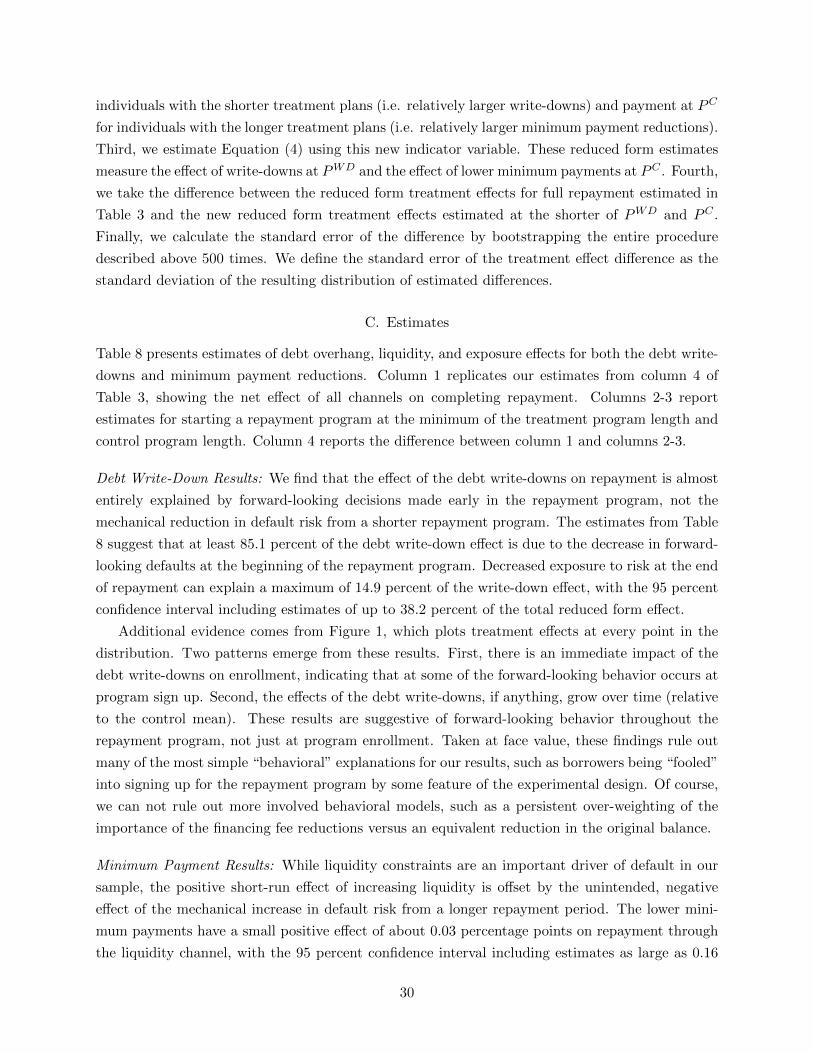
individuals with the shorter treatment plans (i.e. relatively larger write-downs) and payment at PC

for individuals with the longer treatment plans (i.e. relatively larger minimum payment reductions).

Third, we estimate Equation (4) using this new indicator variable. These reduced form estimates

measure the effect of write-downs at PWD and the effect of lower minimum payments at PC . Fourth,

we take the difference between the reduced form treatment effects for full repayment estimated in

Table 3 and the new reduced form treatment effects estimated at the shorter of PWD and PC .

Finally, we calculate the standard error of the difference by bootstrapping the entire procedure

described above 500 times. We define the standard error of the treatment effect difference as the

standard deviation of the resulting distribution of estimated differences.

C. Estimates

Table 8 presents estimates of debt overhang, liquidity, and exposure effects for both the debt write-

downs and minimum payment reductions. Column 1 replicates our estimates from column 4 of

Table 3, showing the net effect of all channels on completing repayment. Columns 2-3 report

estimates for starting a repayment program at the minimum of the treatment program length and

control program length. Column 4 reports the difference between column 1 and columns 2-3.

Debt Write-Down Results: We find that the effect of the debt write-downs on repayment is almost

entirely explained by forward-looking decisions made early in the repayment program, not the

mechanical reduction in default risk from a shorter repayment program. The estimates from Table

8 suggest that at least 85.1 percent of the debt write-down effect is due to the decrease in forward-

looking defaults at the beginning of the repayment program. Decreased exposure to risk at the end

of repayment can explain a maximum of 14.9 percent of the write-down effect, with the 95 percent

confidence interval including estimates of up to 38.2 percent of the total reduced form effect.

Additional evidence comes from Figure 1, which plots treatment effects at every point in the

distribution. Two patterns emerge from these results. First, there is an immediate impact of the

debt write-downs on enrollment, indicating that at some of the forward-looking behavior occurs at

program sign up. Second, the effects of the debt write-downs, if anything, grow over time (relative

to the control mean). These results are suggestive of forward-looking behavior throughout the

repayment program, not just at program enrollment. Taken at face value, these findings rule out

many of the most simple “behavioral” explanations for our results, such as borrowers being “fooled”

into signing up for the repayment program by some feature of the experimental design. Of course,

we can not rule out more involved behavioral models, such as a persistent over-weighting of the

importance of the financing fee reductions versus an equivalent reduction in the original balance.

Minimum Payment Results: While liquidity constraints are an important driver of default in our

sample, the positive short-run effect of increasing liquidity is offset by the unintended, negative

effect of the mechanical increase in default risk from a longer repayment period. The lower mini-

mum payments have a small positive effect of about 0.03 percentage points on repayment through

the liquidity channel, with the 95 percent confidence interval including estimates as large as 0.16

30

percentage points. In all specifications, however, any positive effect from increased liquidity is

nearly exactly offset by the negative effect of increased exposure to default risk. These estimates

are also consistent with the patterns observed in Figure 1, where we see a small positive effect of

lower minimum payments in the short run and small negative effects in the long run.

We view these results as suggesting that the null effect of the minimum payment reductions is

due to the unintended negative effect of exposing individuals to more default risk at the end of the

repayment program. This interpretation of the results is also consistent with the prior literature

suggesting that liquidity constraints and present-bias are important determinants of individual

behavior. We also emphasize that our modest point estimates for the liquidity effect may be due to

the relatively small payment reductions offered to treated individuals. It is possible that distressed

borrowers benefit disproportionately more from larger increases in liquidity, such as those generated

by the mortgage rate resets examined in the recent literature (e.g., Di Maggio et al. 2014, Keys et

al. 2014, Fuster and Willen 2015).

VI. Conclusion

This paper uses information from a large-scale randomized experiment to estimate the independent

effects of debt relief targeting short- and long-run financial constraints. We find significant positive

effects of debt write-downs meant to address longer-run debt overhang, particularly for the highest-

debt borrowers. In contrast, we find no effects of immediate payment reductions meant to address

short-run liquidity constraints. These results stand in stark contrast to the widespread view that

short-run financial constraints are the most important driver of borrower distress.

Our results are of particular importance in light of the ongoing debate on the relative merits

of different types of debt relief. For example, current banking regulations in the United States

prevent credit card issuers from offering more generous debt write-downs, at least in part due

to the perceived unimportance of longer-run constraints such as debt overhang.14,15 During the

financial crisis, a group of credit card issuers asked for these regulations to be relaxed so that

they could conduct a pilot program forgiving up to 40 percent of a credit card borrower’s original

principal (while restructuring the remaining principal to be repaid over a number of years and

deferring any income taxes owed on the forgiven principal). Our results suggest that there may be

substantial benefits of considering such pilot programs.

An important limitation of our analysis is that we are not able to estimate the impact of targeted

14Specifically, U.S. banking regulations prevent credit card issuers from simultaneously reducing the original prin-cipal and lengthening the repayment period unless a debt is first classified as impaired. If the original principal isreduced without the debt being classified as impaired, borrowers are required to pay off the remaining debt in just afew months. Government regulators justify these restrictions based on concerns about when delinquent debts wouldbe recognized on the card issuers’ balance sheets.

15There was an analogous debate regarding targeted debt relief for mortgage borrowers during the fi-nancial crisis. For example, former Treasury Secretary Timothy Geithner wrote in his memoir that thegovernment’s “biggest debate [during the financial crisis] was whether to try to reduce overall mort-gage loans or just monthly payments.” See also https://www.washingtonpost.com/business/economy/

economists-obama-administration-at-odds-over-role-of-mortgage-debt-in-slow-recovery/2012/11/22/

dc83f25e-2e87-11e2-89d4-040c9330702a_story.html

31

debt relief on ex-ante borrower behavior or ex-ante borrowing costs. There may also be important

ex-post impacts of targeted debt relief on outcomes such as post-repayment interest rates that we

are unable to measure with our data. Finally, we are unable to test whether the forward-looking

decisions documented in this paper are due to rational or non-rational decision making. These

questions remain important areas for future research.

32

References

[1] Adams, William, Liran Einav, and Jonathan Levin. 2009. “Liquidity Constraints and Imperfect

Information in Subprime Lending.” American Economic Review, 99(1): 49-84.

[2] Adelino, Manuel, Antoinette Schoar, and Felipe Severino. 2013. “House Prices, Collateral and

Self-Employment.” NBER Working Paper No. 18868.

[3] Agarwal, Sumit, Gene Amromin, Itzhak Ben-David, Souphala Chomsisengphet, Tomasz Pisko-

rski, and Amit Seru. 2012. “Policy Intervention in Debt Renegotiation: Evidence from the

Home Affordable Modification Program.” NBER Working Paper No. 18311.

[4] Agarwal, Sumit, Nicholas Souleles, and Chunlin Liu. 2007. “The Reaction of Consumer Spend-

ing and Debt to Tax Rebates – Evidence from Consumer Credit Data.” Journal of Political

Economy, 115(6): 986-1019.

[5] Agarwal, Sumit, Souphala Chomsisengphet, Neale Mahoney, and Johannes Stroebel. 2015.

“Regulating Consumer Financial Products: Evidence from Credit Cards.” Quarterly Journal

of Economics, 130(1): 111-164.

[6] Autor, David H., David Dorn, and Gordon H. Hanson. 2013. “The China Syndrome: Local La-

bor Market Effects of Import Competition in the United States.” American Economic Review,

103(6): 2121-2168.

[7] Bartik, Timothy J. 1991. “Who Benefits from State and Local Economic Development Poli-

cies?” Upjohn Institute for Employment Research Working Paper.

[8] Benjamin, David, and Xavier Mateos-Planas. 2014. “Formal versus Informal Default in Con-

sumer Credit.” Unpublished Working Paper.

[9] Bernstein, Asaf. 2016. “Household Debt Overhang and Labor Supply.” Unpublished Working

Paper.

[10] Blanchard, Olivier J., and Lawrence F. Katz. 1992. “Regional Evolutions.” Brookings Papers

on Economic Activity, 23(1): 1-76.

[11] Bos, Marieke, Emily Breza, and Andres Liberman. 2015. “The Labor Market Effects of Credit

Market Information.” Unpublished Working Paper.

[12] Card, David. 2001. “Immigrant Inflows, Native Outflows, and the Local Market Impacts of

Higher Immigration.” Journal of Labor Economics, 19(1): 22-64.

[13] Chatterjee, Satyajit, Dean Corbae, Makoto Nakajima, and Jose-Vıctor Rıos-Rull. 2007. “A

Quantitative Theory of Unsecured Consumer Credit with Risk of Default.” Econometrica,

75(6): 1525-1589.

33

[14] DellaVigna, Stefano. 2009. “Psychology and Economics: Evidence from the Field.” Journal of

Economic Literature, 47(2): 315-372.

[15] Di Maggio, Marco, Amir Kermani, and Rodney Ramcharan. 2014. “Monetary Pass-Through:

Household Consumption and Voluntary Deleveraging.” Unpublished Working Paper.

[16] Dobbie, Will, and Paul Goldsmith-Pinkham. 2014. “Debt Protections and the Great Reces-

sion.” Unpublished Working Paper.

[17] Dobbie, Will, Paul Goldsmith-Pinkham, Neale Mahoney, and Jae Song. 2016. “Bad Credit, No

Problem? Credit and Labor Market Consequences of Bad Credit Reports.” NBER Working

Paper No. 22711.

[18] Dobbie, Will, Paul Goldsmith-Pinkham, and Crystal Yang. “Consumer Bankruptcy and Fi-

nancial Health.” Forthcoming at Review of Economics and Statistics.

[19] Dobbie, Will, and Jae Song. 2015. “Debt Relief and Debtor Outcomes: Measuring the Effects

of Consumer Bankruptcy Protection.” American Economic Review, 105(3): 1272-1311.

[20] Eberly, Janice, and Arvind Krishnamurthy. 2014. “Efficient Credit Policies in a Housing Cri-

sis.” Brookings Papers on Economic Activity, 45(2): 73-136.

[21] Fuster, Andreas, and Paul Willen. 2015. “Payment Size, Negative Equity, and Mortgage De-

fault.” FRB of New York Staff Report No. 582.

[22] Ganong, Peter, and Pascal Noel. 2017. “The Effect of Debt on Default and Consumption:

Evidence from Housing Policy in the Great Recession.” Unpublished Working Paper.

[23] Goldsmith-Pinkham, Paul, Isaac Sorkin, and Henry Swift. 2017. “Bartik Instruments: What,

When, Why and How.” Unpublished Working Paper.

[24] Gross, David, and Nicholas Souleles. 2002. “Do Liquidity Constraints and Interest Rates Mat-

ter for Consumer Behavior? Evidence from Credit Card Data.” Quarterly Journal of Eco-

nomics, 117(1): 149-185.

[25] Gross, Tal, and Matthew J. Notowidigdo. 2011. “Health Insurance and the Consumer

Bankruptcy Decision: Evidence from Expansions of Medicaid.” Journal of Public Economics,

95(7-8): 767-778.

[26] Gross, Tal, Matthew J. Notowidigdo, and Jialan Wang. 2014. “Liquidity Constraints and

Consumer Bankruptcy: Evidence from Tax Rebates.” Review of Economics and Statistics,

96(3): 431-443.

[27] Gross, Tal, Matthew J. Notowidigdo, and Jialan Wang. 2016. “The Marginal Propensity to

Consume over the Business Cycle.” NBER Working Paper No. 22518.

34

[28] Haughwout, Andrew, Ebiere Okah, and Joseph Tracy. 2010. “Second Chances: Subprime

Mortgage Modification and Re-Default.” Federal Reserve Bank of New York Staff Reports No.

417.

[29] Heidhues, Paul, and Boton Koszegi. 2010. “Exploiting Naıvete about Self-Control in the Credit

Market.” American Economic Review, 100(5): 2279-2303.

[30] Herkenhoff, Kyle. 2013. “The Impact of Consumer Credit Access on Job Finding Rates.”

Unpublished Working Paper.

[31] Herkenhoff, Kyle, and Gordon Phillips. 2015. “How Credit Constraints Impact Job Finding

Rates, Sorting, and Aggregate Output.” Unpublished Working Paper.

[32] Hunt, Robert M. 2005. “Whither Consumer Credit Counseling?” Federal Reserve Bank of

Philadelphia Business Review, 4Q.

[33] Johnson, David, Jonathan Parker, and Nicholas Souleles. 2006. “Household Expenditure and

the Income Tax Rebates of 2001.” American Economic Review, 96(5): 1589-1610.

[34] Karlan, Dean, and Jonathan Zinman. 2009. “Observing Unobservables: Identifying Informa-

tion Asymmetries with a Consumer Credit Field Experiment.” Econometrica, 77(6): 1993-

2008.

[35] Keys, Benjamin J., Tomasz Piskorski, Amit Seru, and Vincent Yao. 2014. “Mortgage Rates,

Household Balance Sheets, and the Real Economy.” Columbia Business School Research Paper

No. 14-53.

[36] Li, Wenli, Michelle J. White, and Ning Zhu. 2011. “Did Bankruptcy Reform Cause Mortgage

Defaults to Rise?” American Economic Journal: Economic Policy, 3(4): 123-147.

[37] Laibson, David. 1997. “Golden Eggs and Hyperbolic Discounting.” Quarterly Journal of Eco-

nomics, 112(2): 443-478.

[38] Laibson, David, Peter Maxted, Andrea Repetto, and Jeremy Tobacman. 2017. “Estimating

Discount Functions with Consumption Choices over the Lifecycle.” Unpublished Working Pa-

per.

[39] Liberman, Andres. “The Value of a Good Credit Reputation: Evidence from Credit Card

Renegotiations.” Forthcoming in Journal of Financial Economics.

[40] Lusardi, Annamaria, Daniel J. Schneider, and Peter Tufano. 2011. “Financially Fragile House-

holds: Evidence and Implications.” NBER Working Paper No. 17072.

[41] Mahoney, Neale. 2015. “Bankruptcy as Implicit Health Insurance.” American Economic Re-

view, 105(2): 710-764.

35

[42] Meier, Stephan, and Charles Sprenger. 2010. “Present-Biased Preferences and Credit Card

Borrowing.” American Economic Journal: Applied Economics, 2(1): 193-210.

[43] Melzer, Brian. “Mortgage Debt Overhang: Reduced Investment by Homeowners with Negative

Equity.” Forthcoming in Journal of Finance.

[44] Mullainathan, Senhil, and Eldar Shafir. 2013. Scarcity: Why Having Too Little Means So

Much. Macmillan.

[45] O’Neill, Barbara, Aimee D. Prawitz, Benoit Sorhaindo, Jinhee Kim, and E. Thomas Garman.

2006. “Changes in Health, Negative Financial Events, and Financial Distress/Financial Well-

Being for Debt Management Program Clients.” Financial Counseling and Planning, 17(2):

46-63.

[46] Parker, Jonathan, Nicholas Souleles, David Johnson, and Robert McClelland. 2013. “Consumer

Spending and the Economic Stimulus Payments of 2008.” American Economic Review, 103(6):

2530-2553.

[47] Schmieder, Johannes F., Till von Wacther, and Stefan Bender. 2016. “The Effect of Unem-

ployment Benefits and Nonemployment Durations on Wages.” American Economic Review,

106(3): 739-777.

[48] Staten, Michael E., and John M. Barron. 2006. “Evaluating the Effectiveness of Credit Coun-

seling.” Unpublished Working Paper.

[49] Wilshusen, Stephanie. 2011. “Meeting the Demand for Debt Relief.” Federal Reserve Bank of

Philadelphia Payment Cards Center Discussion Paper, 11-04.

[50] Zinman, Jonathan. 2015. “Household Debt: Facts, Puzzles, Theories, and Policies.” Annual

Review of Economics, 7: 251-276

36

Table 1: Examples of the Randomized Treatments

Treatments Program Characteristics Discounted Cost to LenderDebt Payment Minimum Financing Total 0% Disc. 8.5% Disc. 20% Disc.

Write-Down Reduction Payment Costs Months Rate Rate Rate(1) (2) (3) (4) (5) (6) (7) (8)– – $433.45 $3,482 50.05 – – –

∆3.69% – $433.45 $1,770 46.10 $1,221 $802 $440– ∆0.14% $406.77 $3,771 54.04 $159 $332 $444

Notes: This table describes the effect of treatment eligibility on repayment program attributes and lender costs.Minimum payment is the minimum required payment of the program. Financing costs include the total cost of allinterest rate payments and late fees. Total months is the total number of months before the program is complete.All program characteristics and lender costs are calculated using the control means for debt ($18,212), minimumpayment (2.38% of debt), and interest rate (8.5%). The net present value (NPV) of lender costs (relative to thebaseline case) using the control mean for the monthly default rate during the repayment program (1.12%) and usingdiscount rates of 0%, 8.5%, and 20%. The first row reports program characteristics for the baseline case with notreatments. The second row reports program characteristics after the 50th percentile debt write-down treatmentin terms of the implied interest rate cut. The third row reports program characteristics after the 50th percentileminimum payment treatment in terms of the percentage point decrease in the required payment.

37

Table 2: Descriptive Statistics and Balance Tests

Treatment Control DifferencePanel A: Characteristics (1) (2) (3)

Age 40.626 40.516 −0.271Male 0.363 0.361 0.008White 0.636 0.635 0.010Black 0.171 0.174 −0.008∗

Hispanic 0.090 0.088 −0.001Homeowner 0.412 0.410 −0.003Renter 0.440 0.442 0.003Dependents 2.159 2.156 −0.006Monthly Income 2.453 2.448 0.010Monthly Expenses 2.168 2.158 0.003Total Unsecured Debt 18.212 18.368 0.299Debt with Part. Creditors 9.568 9.615 0.163Internal Risk Score -0.000 -0.003 −0.003

Panel B: Baseline OutcomesBankruptcy 0.004 0.003 −0.001Nonzero Collections Debt 0.253 0.254 −0.001Credit Score 585.661 584.991 0.182Employment 0.848 0.850 0.004Earnings 23.447 23.518 −0.108Nonzero 401k Cont. 0.227 0.224 −0.006401k Contributions 0.372 0.373 −0.008

Panel C: Data QualityMatched to SSA data 0.953 0.954 0.003Matched to TU Data 0.899 0.895 −0.001

Panel D: Potential Treatment IntensityInterest Rate if Control 0.085 0.084 0.001Interest Rate if Treatment 0.059 0.060 −0.001Min. Payment Percent if Control 0.024 0.024 −0.001Min. Payment Percent if Treatment 0.023 0.023 −0.000Program Length in Months if Control 52.671 52.678 0.058Program Length in Months if Treatment 51.963 51.914 0.036

Panel E: Characteristics of Repayment ProgramInterest Rate 0.085 0.059 −0.026∗∗∗

Min. Payment Percent 0.024 0.023 −0.001∗∗∗

Program Length in Months 52.671 51.914 −0.806∗∗∗

p-value from joint F-test of Panels A-D – – 0.991p-value from joint F-test of Panel E – – 0.000Observations 40,496 39,243 79,739

Notes: This table reports descriptive statistics and balance tests for the estimation sample. Information on age,gender, race, earnings, employment, and 401k contributions is only available for individuals matched to the SSA dataand information on collections debt and credit score are only available for individuals matched to the TU data. Eachbaseline outcome is for the year before the experiment. Potential minimum payment and interest rates are calculatedusing the amount of debt held by each creditor and the rules listed in Appendix Table 1. All dollar amounts aredivided by 1,000. Column 3 reports the difference between the treatment and control groups, controlling for stratafixed effects and clustering standard errors at the counselor level. *** = significant at 1 percent level, ** = significantat 5 percent level, * = significant at 10 percent level. The p-value is from an F-test of the joint significance of thevariables listed.

38

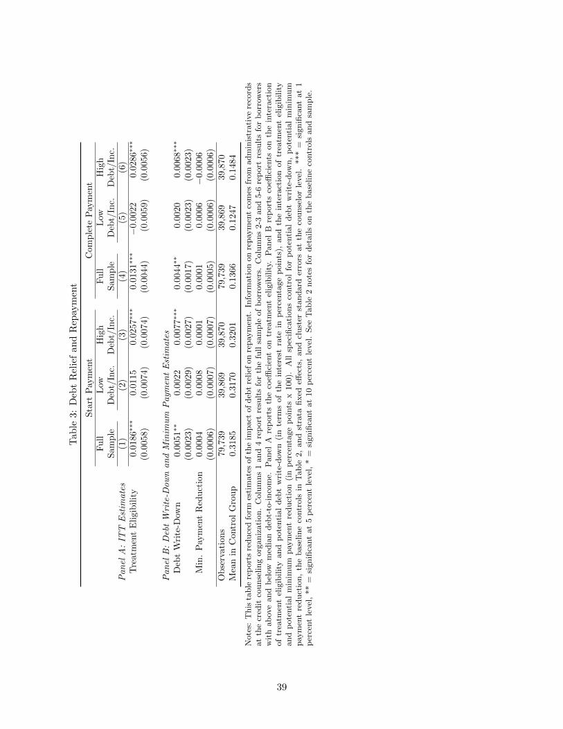
Tab

le3:

Deb

tR

elie

fan

dR

epay

men

t

Sta

rtP

aym

ent

Com

ple

teP

aym

ent

Fu

llL

owH

igh

Fu

llL

owH

igh

Sam

ple

Deb

t/In

c.D

ebt/

Inc.

Sam

ple

Deb

t/In

c.D

ebt/

Inc.

Pan

elA

:IT

TE

stim

ate

s(1

)(2

)(3

)(4

)(5

)(6

)T

reat

men

tE

ligi

bil

ity

0.0186∗

∗∗0.

0115

0.0257∗

∗∗0.0

131∗

∗∗−

0.00

22

0.0286∗∗

∗

(0.0

058)

(0.0

074)

(0.0

074)

(0.0

044)

(0.0

059)

(0.0

056)

Pan

elB

:D

ebt

Wri

te-D

ow

nan

dM

inim

um

Paym

ent

Est

imate

sD

ebt

Wri

te-D

own

0.0051∗

∗0.

0022

0.0077∗

∗∗0.0

044∗

∗0.

0020

0.0068∗∗

∗

(0.0

023)

(0.0

029)

(0.0

027)

(0.0

017)

(0.0

023)

(0.0

023)

Min

.P

aym

ent

Red

uct

ion

0.0

004

0.0008

0.0001

0.0001

0.0006

−0.

0006

(0.0

006)

(0.0

007)

(0.0

007)

(0.0

005)

(0.0

006)

(0.0

006)

Ob

serv

atio

ns

79,7

39

39,8

69

39,8

70

79,7

39

39,8

69

39,8

70

Mea

nin

Con

trol

Gro

up

0.3

185

0.3

170

0.3

201

0.1

366

0.1

247

0.1

484

Note

s:T

his

table

rep

ort

sre

duce

dfo

rmes

tim

ate

sof

the

impact

of

deb

tre

lief

on

repay

men

t.In

form

ati

on

on

repay

men

tco

mes

from

adm

inis

trati

ve

reco

rds

at

the

cred

itco

unse

ling

org

aniz

ati

on.

Colu

mns

1and

4re

port

resu

lts

for

the

full

sam

ple

of

borr

ower

s.C

olu

mns

2-3

and

5-6

rep

ort

resu

lts

for

borr

ower

sw

ith

ab

ove

and

bel

owm

edia

ndeb

t-to

-inco

me.

Panel

Are

port

sth

eco

effici

ent

on

trea

tmen

tel

igib

ilit

y.P

anel

Bre

port

sco

effici

ents

on

the

inte

ract

ion

of

trea

tmen

tel

igib

ilit

yand

pote

nti

al

deb

tw

rite

-dow

n(i

nte

rms

of

the

inte

rest

rate

inp

erce

nta

ge

poin

ts),

and

the

inte

ract

ion

of

trea

tmen

tel

igib

ilit

yand

pote

nti

al

min

imum

pay

men

tre

duct

ion

(in

per

centa

ge

poin

tsx

100).

All

spec

ifica

tions

contr

ol

for

pote

nti

al

deb

tw

rite

-dow

n,

pote

nti

al

min

imum

pay

men

tre

duct

ion,

the

base

line

contr

ols

inT

able

2,

and

stra

tafixed

effec

ts,

and

clust

erst

andard

erro

rsat

the

counse

lor

level

.***

=si

gnifi

cant

at

1p

erce

nt

level

,**

=si

gnifi

cant

at

5p

erce

nt

level

,*

=si

gnifi

cant

at

10

per

cent

level

.See

Table

2note

sfo

rdet

ails

on

the

base

line

contr

ols

and

sam

ple

.

39

Table 4: Debt Relief and Bankruptcy Filing

Bankruptcy in Years 1-5Full Low High

Sample Debt/Inc. Debt/Inc.Panel A: ITT Estimates (1) (2) (3)

Treatment Eligibility −0.0030 0.0054 −0.0113∗∗∗

(0.0035) (0.0050) (0.0040)

Panel B: Debt Write-Down and Minimum Payment EstimatesDebt Write-Down −0.0027∗∗ −0.0016 −0.0036∗∗

(0.0014) (0.0015) (0.0019)Min. Payment Reduction 0.0005 0.0002 0.0007

(0.0003) (0.0004) (0.0004)Observations 79,739 39,869 39,870Mean in Control Group 0.1036 0.0658 0.1416

Notes: This table reports reduced form estimates of the impact of debt relief on bankruptcy. Information onbankruptcy comes from court records. Column 1 reports results for the full sample of borrowers. Columns 2-3report results for borrowers with above and below median debt-to-income. Panel A reports the coefficient on treat-ment eligibility. Panel B reports coefficients on the interaction of treatment eligibility and potential debt write-down(in terms of the interest rate in percentage points), and the interaction of treatment eligibility and potential minimumpayment reduction (in percentage points x 100). All specifications control for potential debt write-down, potentialminimum payment reduction, the baseline controls in Table 2, and strata fixed effects, and cluster standard errorsat the counselor level. *** = significant at 1 percent level, ** = significant at 5 percent level, * = significant at 10percent level. See Table 2 notes for details on the baseline controls and sample.

40

Tab

le5:

Deb

tR

elie

fan

dF

inan

cial

Ou

tcom

es

Non

zero

Coll

ecti

on

sD

ebt

Cre

dit

Sco

reF

ull

Low

Hig

hF

ull

Low

Hig

hS

am

ple

Deb

t/In

c.D

ebt/

Inc.

Sam

ple

Deb

t/In

c.D

ebt/

Inc.

Pan

elA

:IT

TE

stim

ate

s(1

)(2

)(3

)(4

)(5

)(6

)T

reat

men

tE

ligi

bil

ity

0.0007

0.0091

−0.0

076∗

−0.

2195

−0.

7046

3.2585∗

∗∗

(0.0

046)

(0.0

057)

(0.0

044)

(0.7

537)

(1.0

352)

(0.9

855)

Pan

elB

:D

ebt

Wri

te-D

ow

nan

dM

inim

um

Paym

ent

Deb

tW

rite

-Dow

n−

0.0034∗

−0.

0047∗∗−

0.0

023

0.5278

0.6617

0.4602

(0.0

019)

(0.0

024)

(0.0

023)

(0.3

422)

(0.4

452)

(0.4

063)

Min

.P

aym

ent

Red

uct

ion

0.0

010∗

∗0.

0010∗

0.0

009∗

−0.

1270

−0.

0297∗−

0.2

042∗

∗

(0.0

005)

(0.0

006)

(0.0

005)

(0.0

862)

(0.1

151)

(0.0

949)

Ob

serv

atio

ns

71,5

16

35,3

54

36,1

62

71,5

16

35,3

54

36,1

62

Mea

nin

Con

trol

Gro

up

0.3

929

0.4

659

0.3

213

603.0

766

586.9

836

618.9

447

Note

s:T

his

table

rep

ort

sre

duce

dfo

rmes

tim

ate

sof

the

impact

of

deb

tre

lief

on

hav

ing

any

collec

tions

deb

tand

cred

itsc

ore

.In

form

ati

on

on

outc

om

esco

mes

from

cred

itre

cord

sat

Tra

nsU

nio

n.

Colu

mns

1and

4re

port

resu

lts

for

the

full

sam

ple

of

borr

ower

s.C

olu

mns

2-3

and

5-6

rep

ort

resu

lts

for

borr

ower

sw

ith

ab

ove

and

bel

owm

edia

ndeb

t-to

-inco

me.

Panel

Are

port

sth

eco

effici

ent

on

trea

tmen

tel

igib

ilit

y.P

anel

Bre

port

sco

effici

ents

on

the

inte

ract

ion

of

trea

tmen

tel

igib

ilit

yand

pote

nti

al

deb

tw

rite

-dow

n(i

nte

rms

of

the

inte

rest

rate

inp

erce

nta

ge

poin

ts),

and

the

inte

ract

ion

of

trea

tmen

tel

igib

ilit

yand

pote

nti

al

min

imum

pay

men

tre

duct

ion

(in

per

centa

ge

poin

tsx

100).

All

spec

ifica

tions

contr

ol

for

pote

nti

al

deb

tw

rite

-dow

n,

pote

nti

al

min

imum

pay

men

tre

duct

ion,

the

base

line

contr

ols

inT

able

2,

and

stra

tafixed

effec

ts,

and

clust

erst

andard

erro

rsat

the

counse

lor

level

.***

=si

gnifi

cant

at

1p

erce

nt

level

,**

=si

gnifi

cant

at

5p

erce

nt

level

,*

=si

gnifi

cant

at

10

per

cent

level

.See

Table

2note

sfo

rdet

ails

on

the

base

line

contr

ols

and

sam

ple

.

41

Tab

le6:

Deb

tR

elie

fan

dL

abor

Mar

ket

Ou

tcom

es

Em

plo

ym

ent

Earn

ings

Fu

llL

owH

igh

Fu

llL

owH

igh

Sam

ple

Deb

t/In

c.D

ebt/

Inc.

Sam

ple

Deb

t/In

c.D

ebt/

Inc.

Pan

elA

:IT

TE

stim

ate

s(1

)(2

)(3

)(4

)(5

)(6

)T

reat

men

tE

ligi

bil

ity

−0.

0018

−0.

0009

−0.0

028

0.0567

−0.

0799

0.1942

(0.0

026)

(0.0

034)

(0.0

035)

(0.1

746)

(0.2

245)

(0.2

191)

Pan

elB

:D

ebt

Wri

te-D

ow

nan

dM

inim

um

Paym

ent

Est

imate

sD

ebt

Wri

te-D

own

0.0003

0.0010

0.0045∗

∗−

0.0390

0.02

64

−0.0

959

(0.0

010)

(0.0

013)

(0.0

021)

(0.0

691)

(0.0

983)

(0.0

774)

Min

.P

aym

ent

Red

uct

ion−

0.0004

−0.

0006∗

−0.0

001

0.0046

0.00

04

0.0

094

(0.0

003)

(0.0

003)

(0.0

003)

(0.0

183)

(0.0

243)

(0.0

215)

Ob

serv

atio

ns

76,0

08

37,8

67

38,1

41

76,0

08

37,8

67

38,1

41

Mea

nin

Con

trol

Gro

up

0.8

202

0.8

586

0.7

819

26.8

915

27.6

506

26.1

331

Note

s:T

his

table

rep

ort

sre

duce

dfo

rmes

tim

ate

sof

the

impact

of

deb

tre

lief

on

emplo

ym

ent

and

earn

ings.

Info

rmati

on

on

outc

om

esco

mes

from

reco

rds

at

the

Soci

al

Sec

uri

tyA

dm

inis

trati

on.

Colu

mns

1and

4re

port

resu

lts

for

the

full

sam

ple

of

borr

ower

s.C

olu

mns

2-3

and

5-6

rep

ort

resu

lts

for

borr

ower

sw

ith

ab

ove

and

bel

owm

edia

ndeb

t-to

-inco

me.

Panel

Are

port

sth

eco

effici

ent

on

trea

tmen

tel

igib

ilit

y.P

anel

Bre

port

sco

effici

ents

on

the

inte

ract

ion

of

trea

tmen

tel

igib

ilit

yand

pote

nti

al

deb

tw

rite

-dow

n(i

nte

rms

of

the

inte

rest

rate

inp

erce

nta

ge

poin

ts),

and

the

inte

ract

ion

of

trea

tmen

tel

igib

ilit

yand

pote

nti

al

min

imum

pay

men

tre

duct

ion

(in

per

centa

ge

poin

tsx

100).

All

spec

ifica

tions

contr

ol

for

pote

nti

al

deb

tw

rite

-dow

n,

pote

nti

al

min

imum

pay

men

tre

duct

ion,

the

base

line

contr

ols

inT

able

2,

and

stra

tafixed

effec

ts,

and

clust

erst

andard

erro

rsat

the

counse

lor

level

.***

=si

gnifi

cant

at

1p

erce

nt

level

,**

=si

gnifi

cant

at

5p

erce

nt

level

,*

=si

gnifi

cant

at

10

per

cent

level

.See

Table

2note

sfo

rdet

ails

on

the

base

line

contr

ols

and

sam

ple

.

42

Tab

le7:

Deb

tR

elie

fan

d40

1kC

ontr

ibu

tion

s

Non

zero

401k

Contr

ibu

tion

s401k

Contr

ibu

tion

sF

ull

Low

Hig

hF

ull

Low

Hig

hS

am

ple

Deb

t/In

c.D

ebt/

Inc.

Sam

ple

Deb

t/In

c.D

ebt/

Inc.

Pan

elA

:IT

TE

stim

ate

s(1

)(2

)(3

)(4

)(5

)(6

)T

reat

men

tE

ligi

bil

ity

0.0012

0.0003

0.0020

0.0010

−0.0

098

0.0118

(0.0

041)

(0.0

058)

(0.0

051)

(0.0

101)

(0.0

131)

(0.0

117)

Pan

elB

:D

ebt

Wri

te-D

ow

nan

dM

inim

um

Paym

ent

Deb

tW

rite

-Dow

n0.

0003

0.0006

0.0001

−0.

0053

−0.

0067

−0.

0038

(0.0

017)

(0.0

022)

(0.0

023)

(0.0

041)

(0.0

056)

(0.0

051)

Min

.P

aym

ent

Red

uct

ion−

0.0001

−0.

0001

−0.0

001

0.0011

0.0017

0.0006

(0.0

004)

(0.0

005)

(0.0

005)

(0.0

010)

(0.0

013)

(0.0

011)

Ob

serv

atio

ns

76,0

08

37,8

67

38,1

41

76,0

08

37,8

67

38,1

41

Mea

nin

Con

trol

Gro

up

0.2

723

0.2

784

0.2

662

0.4

643

0.4

413

0.4

872

Note

s:T

his

table

rep

ort

sre

duce

dfo

rmes

tim

ate

sof

the

impact

of

deb

tre

lief

on

401k

contr

ibuti

ons.

Info

rmati

on

on

all

outc

om

esco

mes

from

reco

rds

at

the

Soci

al

Sec

uri

tyA

dm

inis

trati

on.

Colu

mns

1and

4re

port

resu

lts

for

the

full

sam

ple

of

borr

ower

s.C

olu

mns

2-3

and

5-6

rep

ort

resu

lts

for

borr

ower

sw

ith

ab

ove

and

bel

owm

edia

ndeb

t-to

-inco

me.

Panel

Are

port

sth

eco

effici

ent

on

trea

tmen

tel

igib

ilit

y.P

anel

Bre

port

sco

effici

ents

on

the

inte

ract

ion

of

trea

tmen

tel

igib

ilit

yand

pote

nti

al

deb

tw

rite

-dow

n(i

nte

rms

of

the

inte

rest

rate

inp

erce

nta

ge

poin

ts),

and

the

inte

ract

ion

of

trea

tmen

tel

igib

ilit

yand

pote

nti

al

min

imum

pay

men

tre

duct

ion

(in

per

centa

ge

poin

tsx

100).

All

spec

ifica

tions

contr

ol

for

pote

nti

al

deb

tw

rite

-dow

n,

pote

nti

al

min

imum

pay

men

tre

duct

ion,

the

base

line

contr

ols

inT

able

2,

and

stra

tafixed

effec

ts,

and

clust

erst

andard

erro

rsat

the

counse

lor

level

.***

=si

gnifi

cant

at

1p

erce

nt

level

,**

=si

gnifi

cant

at

5p

erce

nt

level

,*

=si

gnifi

cant

at

10

per

cent

level

.See

Table

2note

sfo

rdet

ails

on

the

base

line

contr

ols

and

sam

ple

.

43

Table 8: Forward-Looking, Liquidity, and Exposure Effects

Total Forward Liquidity ExposureEffect Looking Effect Effect

(1) (2) (3) (4)Debt Write-Down 0.00444∗∗∗ 0.00378∗∗ 0.00066

(0.00174) (0.00184) (0.00053)Min. Payment Reduction 0.00001 0.00018 −0.00017

(0.00048) (0.00048) (0.00011)

Notes: This table reports the forward-looking, liquidity, and exposure effects of each treatment. Column 1 reportsresults for fully completing debt repayment. Columns 2-3 reports results for being enrolled in the repayment programat the minimum of the treatment program length or the control program length. All specifications control for potentialdebt write-down, potential minimum payment reduction, the baseline controls in Table 2, and strata fixed effects.Standard errors for column 4 are calculated using the bootstrap procedure described in the text. *** = significantat 1 percent level, ** = significant at 5 percent level, * = significant at 10 percent level. See the text for additionaldetails on the estimation procedure.

44

Figure 1: Debt Relief and Repayment Rates

Panel A: Debt Write-Down Panel B: Minimum Payment Reduction.1

.15

.2.2

5.3

.35

Frac

tion

0 25 50 75 100Percent of Debt Repaid

Control Mean Interest Reduction

.1.1

5.2

.25

.3.3

5Fr

actio

n

0 25 50 75 100Percent of Debt Repaid

Control Mean Payment Reduction

Notes: These figures report the control mean and implied treatment group means for debt repayment. We calculateeach treatment group mean using the control mean and the reduced form estimates described in Table 3. The shadedregions indicate the 95 percent confidence intervals. All specifications control for the potential minimum payment andwrite-down changes if treated and cluster standard errors at the counselor level. See the Table 3 notes for additionaldetails on the sample and specification.

45

Appendix Table 1: Creditor Concessions and Dates of Participation

Interest Rates Minimum PaymentsCreditor Treatment Control Treatment Control Dates of Participation

1 1.00% 7.30% 2.00% 2.00% Jan. 2005 to Aug. 20062 0.00% 9.90% 1.80% 2.20% Jan. 2005 to Aug. 20063 0.00% 9.00% 1.80% 2.00% Jan. 2005 to Aug. 20064 0.00% 8.00% 2.44% 2.44% Feb. 2005 to Aug. 20065 2.00% 6.00% 1.80% 2.30% Jan. 2005 to Aug. 20066 0.00% 9.90% 2.25% 2.25% Apr. 2005 to Aug. 20067 1.00% 10.00% 1.80% 2.00% May 2005 to Oct. 20058 2.00% 6.00% 1.80% 2.30% Sept. 2005 to Aug. 20069 0.00% 9.90% 1.80% 2.20% Jan. 2005 to Aug. 200610 0.00% 9.90% 1.80% 2.20% Jan. 2005 to Aug. 200611 0.00% 9.90% 1.80% 2.20% Jan. 2005 to Aug. 2006

Notes: This table details the terms offered to the treatment and control groups by the 11 creditors participating inthe randomized trial. Minimum monthly payments are a percentage of the total debt enrolled. See text for additionaldetails.

46

Appendix Table 2: Results with No Baseline Controls

Complete Collections Credit NonzeroPayment Bankrupt Debt Score Employed 401k

Panel A: ITT Estimates (1) (2) (3) (4) (5) (6)Treatment Eligibility 0.0134∗∗∗ −0.0021 −0.0002 −0.0663 0.0023 0.0002

(0.0047) (0.0036) (0.0054) (0.9428) (0.0039) (0.0048)

Panel B: Debt Write-Down and Minimum PaymentDebt Write-Down 0.0049∗∗∗ −0.0024∗ −0.0035∗ 0.5911 0.0022 0.0004

(0.0018) (0.0014) (0.0021) (0.3707) (0.0017) (0.0022)Min. Payment Reduction −0.0001 0.0005 0.0008∗ −0.0985 −0.0007 −0.0002

(0.0005) (0.0003) (0.0005) (0.0951) (0.0005) (0.0005)Observations 79,739 79,739 71,516 71,516 76,008 76,008Mean in Control Group 0.1366 0.1036 0.3929 603.0766 0.8202 0.2723

Notes: This table reports reduced form estimates with no baseline controls. Panel A reports the coefficient ontreatment eligibility. Panel B reports coefficients on the interaction of treatment eligibility and potential debt write-down (in terms of the interest rate in percentage points), and the interaction of treatment eligibility and potentialminimum payment reduction (in percentage points x 100). All specifications control for potential debt write-down,potential monthly minimum reduction, and strata fixed effects, and cluster standard errors at the counselor level.*** = significant at 1 percent level, ** = significant at 5 percent level, * = significant at 10 percent level. See Table2 notes for details on the sample.

47

Ap

pen

dix

Tab

le3:

Non

-Par

amet

ric

Res

ult

s

Com

ple

teC

oll

ecti

ons

Cre

dit

Non

zero

Pay

men

tB

an

kru

pt

Deb

tS

core

Em

plo

yed

401k

(1)

(2)

(3)

(4)

(5)

(6)

Tre

atm

ent

xN

oR

edu

ctio

ns

−0.

0027

0.0030

0.0063

−1.0

877

−0.

0015

0.0002

(0.0

064)

(0.0

054)

(0.0

072)

(1.2

538)

(0.0

049)

(0.0

074)

Tre

atm

ent

xL

owW

rite

-Dow

nx

Low

Pay

men

t0.

0208∗∗−

0.0076

−0.

0096

1.2971

0.0057

0.0054

(0.0

090)

(0.0

075)

(0.0

084)

(1.4

916)

(0.0

050)

(0.0

079)

Tre

atm

ent

xL

owW

rite

-Dow

nx

Hig

hP

aym

ent

0.0

282∗∗

0.0015

−0.

0152

2.1956

−0.

0006

0.0050

(0.0

124)

(0.0

105)

(0.0

125)

(2.0

919)

(0.0

068)

(0.0

117)

Tre

atm

ent

xH

igh

Wri

te-D

own

xL

owP

aym

ent

0.0

156

0.0065

0.0233

−0.7

674

−0.

0004

−0.

0082

(0.0

171)

(0.0

142)

(0.0

152)

(1.8

131)

(0.0

114)

(0.0

159)

Tre

atm

ent

xH

igh

Wri

te-D

own

xH

igh

Pay

men

t0.0

254∗∗−

0.0131∗

0.0085

5.5177∗

−0.

0136∗∗−

0.0020

(0.0

105)

(0.0

078)

(0.0

106)

(3.2

213)

(0.0

063)

(0.0

106)

Ob

serv

atio

ns

79,7

39

79,7

39

71,5

16

71,5

16

76,0

08

76,0

08

Mea

nin

Con

trol

Gro

up

0.1

366

0.1

036

0.3

929

603.0

766

0.8

202

0.2

723

Note

s:T

his

table

rep

ort

ses

tim

ate

sse

para

tely

by

trea

tmen

tin

tensi

tybin

.W

ere

port

coeffi

cien

tson

the

inte

ract

ion

of

trea

tmen

tel

igib

ilit

yand

an

indic

ato

rfo

rhav

ing

pote

nti

al

trea

tmen

tin

tensi

tyin

the

indic

ate

dra

nge.

All

spec

ifica

tions

contr

ol

for

an

exhaust

ive

set

of

pote

nti

al

trea

tmen

tin

tensi

tyfixed

effec

ts,

the

base

line

contr

ols

list

edin

Table

2,

and

stra

tafixed

effec

ts,

and

clust

erst

andard

erro

rsat

the

counse

lor

level

.***

=si

gnifi

cant

at

1p

erce

nt

level

,**

=si

gnifi

cant

at

5p

erce

nt

level

,*

=si

gnifi

cant

at

10

per

cent

level

.

48

Ap

pen

dix

Tab

le4:

Des

crip

tive

Sta

tist

ics

by

Tre

atm

ent

Inte

nsi

ty

Zer

oW

rite

-Dow

nL

owW

rite

-Dow

nL

owW

rite

-Dow

nH

igh

Wri

te-D

own

Hig

hW

rite

-Dow

nx

Zer

oP

aym

ent

xL

owP

aym

ent

xH

igh

Pay

men

tx

Low

Pay

men

tx

Hig

hP

aym

ent

Contr

ol

Diff

.C

ontr

ol

Diff

.C

ontr

ol

Diff

.C

ontr

ol

Diff

.C

ontr

ol

Diff

.Panel

A:Characteristics

(1)

(2)

(3)

(4)

(5)

(6)

(7)

(8)

(9)

(10)

Age

38.4

81

−0.7

35

41.6

95

0.0

10

40.6

24

−0.7

24

44.3

10

0.3

07

41.4

77

0.2

27

Male

0.3

57

0.0

17

0.3

57

0.0

01

0.3

66

0.0

32

0.3

57

0.0

24

0.3

80

0.0

12

Whit

e0.5

72

−0.0

14

0.6

48

0.0

10

0.6

52

0.0

05

0.7

27

0.0

84

0.6

87

0.0

08

Bla

ck0.2

37

−0.0

06

0.1

52

−0.0

06

0.1

41

−0.0

18

0.1

20

−0.0

29

0.1

24

−0.0

22

His

panic

0.0

96

0.0

14

0.0

93

0.0

02

0.0

98

−0.0

09

0.0

68

−0.0

17

0.0

81

−0.0

03

Hom

eow

ner

0.3

16

−0.0

08

0.4

58

0.0

02

0.4

74

−0.0

23

0.5

08

−0.0

18

0.4

43

−0.0

03

Ren

ter

0.5

11

0.0

06

0.4

08

−0.0

18

0.3

90

0.0

15

0.3

66

0.0

21

0.4

17

0.0

17

Dep

enden

ts2.1

55

−0.0

08

2.2

27

−0.0

04

2.1

99

−0.0

14

2.1

60

−0.0

94

2.0

57

−0.0

34

Month

lyIn

com

e2.0

92

0.0

19

2.6

48

−0.0

14

2.6

77

0.0

26

2.6

95

0.0

19

2.5

85

0.0

52

Month

lyE

xp

ense

s1.8

97

0.0

08

2.3

24

−0.0

37

2.3

37

0.0

02

2.3

73

0.0

99

2.2

45

0.0

31

Tota

lU

nse

cure

dD

ebt

10.8

52

−0.1

87

21.8

32

0.6

17

21.7

21

1.0

12

26.3

54

0.1

53

20.7

82

0.9

90

Deb

tw

ith

Part

.C

redit

ors

2.6

34

−0.1

23

8.6

84

0.1

55

14.9

79

0.5

80

15.9

06

−0.4

42

16.6

02

0.8

69

Inte

rnal

Ris

kSco

re0.0

79

−0.0

26

0.1

87

0.0

27

-0.0

72

0.0

76

-0.2

19

0.1

49

-0.2

44

−0.0

43

Panel

B:BaselineOutcomes

Bankru

ptc

y0.0

07

−0.0

02

0.0

03

0.0

01

0.0

02

0.0

01

0.0

00

0.0

03

0.0

02

0.0

01

Cre

dit

Sco

re566.3

53

−0.6

12

582.3

73

1.8

68

596.5

95

−3.1

79

609.8

09

6.5

38

605.8

21

3.4

57

Nonze

roC

ollec

tions

Deb

t0.4

02

0.0

20

0.2

21

−0.0

01

0.1

76

0.0

32

0.1

27

0.0

53

0.1

42

−0.0

37

Em

plo

ym

ent

0.8

48

0.0

12

0.8

52

0.0

02

0.8

70

0.0

21

0.8

21

−0.0

31

0.8

39

−0.0

10

Earn

ings

20.3

98

−0.1

94

25.0

97

−0.4

67

26.0

06

1.2

52

24.3

82

0.0

55

24.5

34

0.7

53

Nonze

ro401k

Cont.

0.1

95

−0.0

05

0.2

43

−0.0

07

0.2

57

0.0

01

0.2

53

−0.0

24

0.2

34

0.0

05

401k

Contr

ibuti

ons

0.2

71

−0.0

12

0.4

00

−0.0

06

0.4

52

−0.0

63

0.4

60

−0.0

57

0.4

22

0.0

21

Panel

C:Data

Quality

Matc

hed

toSSA

data

0.9

53

−0.0

02

0.9

49

0.0

03

0.9

52

−0.0

05

0.9

62

0.0

13

0.9

53

−0.0

01

Matc

hed

toT

UD

ata

0.8

89

−0.0

19∗∗

0.9

02

0.0

08

0.9

01

0.0

01

0.9

13

0.0

36

0.9

03

−0.0

11

Panel

D:PotentialTreatm

entIntensity

Inte

rest

Rate

ifC

ontr

ol

0.0

80

0.0

00

0.0

86

0.0

01

0.0

93

0.0

00

0.0

80

0.0

00

0.0

89

0.0

00

Inte

rest

Rate

ifT

reatm

ent

0.0

80

0.0

00

0.0

68

0.0

00

0.0

34

0.0

02

0.0

55

0.0

00

0.0

27

0.0

00

Min

.P

aym

ent

ifC

ontr

ol

0.0

28

−0.0

00

0.0

25

−0.0

00

0.0

25

−0.0

00

0.0

25

−0.0

00

0.0

25

−0.0

00

Min

.P

aym

ent

ifT

reatm

ent

0.0

28

−0.0

00

0.0

25

−0.0

00

0.0

24

−0.0

00

0.0

22

−0.0

00

0.0

22

−0.0

00

Pro

gra

mL

ength

ifC

ontr

ol

51.3

79

0.0

81

52.6

82

0.0

12

54.8

94

0.4

13

51.7

50

0.3

35

53.7

85

0.1

99

Pro

gra

mL

ength

ifT

reatm

ent

51.4

63

0.0

89

51.6

33

−0.0

29

49.1

36

0.4

49

55.3

86

0.3

52

53.6

44

0.1

09

49

Panel

E:Characteristics

ofRepaym

entProgram

Inte

rest

Rate

0.0

80

0.0

00

0.0

86

−0.0

18∗∗∗

0.0

93

−0.0

57∗∗∗

0.0

80

−0.0

24∗∗∗

0.0

89

−0.0

62∗∗∗

Min

.P

aym

ent

Per

cent

0.0

28

−0.0

00

0.0

25

−0.0

01∗∗∗

0.0

25

−0.0

01∗∗

0.0

25

−0.0

03∗∗∗

0.0

25

−0.0

03∗∗∗

Pro

gra

mL

ength

inM

onth

s51.3

79

0.1

52

52.6

82

−1.1

54∗∗∗

54.8

94

−5.3

47∗∗∗

51.7

50

4.0

14∗∗∗

53.7

85

−0.1

46

join

tF

-tes

tof

Panel

sA

-D–

0.9

98

–0.9

99

–1.0

00

–0.9

88

–0.9

99

join

tF

-tes

tof

Panel

E–

0.8

47

–0.0

00

–0.0

00

–0.0

00

–0.0

00

Obse

rvati

ons

13,7

01

26,9

92

10,5

45

20,6

77

2,9

26

5,6

76

4,9

00

9,8

70

8,4

24

16,5

24

Note

s:T

his

table

rep

ort

ssu

mm

ary

stati

stic

sby

pote

nti

al

trea

tmen

tin

tensi

ty.

See

the

Table

2note

sfo

rdet

ails

on

the

vari

able

defi

nit

ions.

50

Appendix Table 5: Additional Tests of Random Assignment

Control Treated x Treated x p-value onMean ∆ Rate ∆ Payment joint test

(1) (2) (3) (4)Age 40.6256 −0.0314 0.0034 0.8785

(13.4135) (0.0759) (0.0199)Male 0.3631 0.0020 −0.0002 0.7004

(0.4809) (0.0029) (0.0007)White 0.6363 0.0031 −0.0000 0.2217

(0.4811) (0.0026) (0.0006)Black 0.1712 −0.0003 −0.0004 0.1719

(0.3767) (0.0019) (0.0004)Hispanic 0.0904 −0.0027 0.0005 0.2617

(0.2868) (0.0017) (0.0004)Homeowner 0.4123 −0.0019 0.0006 0.5496

(0.4923) (0.0023) (0.0006)Renter 0.4395 0.0024 −0.0007 0.4936

(0.4963) (0.0025) (0.0006)Dependents 2.1590 −0.0017 0.0009 0.8749

(1.3852) (0.0070) (0.0018)Monthly Income 2.4534 0.0066 −0.0012 0.6796

(1.4452) (0.0076) (0.0020)Monthly Expenses 2.1682 0.0014 −0.0001 0.9542

(1.2944) (0.0068) (0.0018)Total Unsecured Debt 18.2120 0.1233 −0.0107 0.1775

(16.9388) (0.0761) (0.0195)Debt with Part. Creditors 9.5679 0.0813 −0.0110 0.3257

(12.6572) (0.0566) (0.0154)Internal Risk Score -0.0000 0.0010 −0.0007 0.8118

(1.0000) (0.0051) (0.0012)Collections Debt 0.2529 0.0022 −0.0009 0.1658

(0.4347) (0.0024) (0.0007)Credit Score 585.6605 −0.0588 0.0588 0.7114

(69.8287) (0.3795) (0.0993)Bankruptcy 0.0038 −0.0002 0.0000 0.7922

(0.0614) (0.0003) (0.0001)Employment 0.8478 0.0028 −0.0005 0.3700

(0.3593) (0.0020) (0.0005)Earnings 23.4466 0.0272 −0.0041 0.9714

(21.1752) (0.1188) (0.0302)Nonzero 401k Cont. 0.2272 −0.0004 −0.0001 0.8762

(0.4190) (0.0023) (0.0006)401k Contributions 0.3717 −0.0019 −0.0002 0.7577

(0.9688) (0.0056) (0.0014)Matched to SSA data 0.9526 0.0005 0.0001 0.5749

(0.2124) (0.0011) (0.0003)Matched to TU Data 0.8985 0.0002 0.0000 0.9747

(0.3019) (0.0015) (0.0004)Observations 40,496 79,739

Notes: This table reports additional tests of random assignment. We report coefficients on the interaction of treatmentand potential treatment intensity. All regressions control for potential treatment intensity and strata fixed effects,and cluster standard errors at the counselor level. Column 4 reports the p-value from an F-test that all interactionsare jointly equal to zero. See Table 2 notes for additional details on the sample and variable construction.

51

Appendix Table 6: Correlates of Potential Treatment Intensity

Control p-value onMean ∆ Rate ∆ Payment joint test

(1) (2) (3) (4)Age 40.6256 0.0281 0.0782∗∗∗ 0.0000

(13.4135) (0.0417) (0.0108)Male 0.3631 0.0020 0.0009∗∗ 0.0000

(0.4809) (0.0015) (0.0004)White 0.6363 0.0070∗∗∗ 0.0023∗∗∗ 0.0000

(0.4811) (0.0016) (0.0004)Black 0.1712 −0.0079∗∗∗ −0.0015∗∗∗ 0.0000

(0.3767) (0.0012) (0.0003)Hispanic 0.0904 −0.0006 −0.0008∗∗∗ 0.0000

(0.2868) (0.0011) (0.0003)Homeowner 0.4123 0.0122∗∗∗ 0.0009∗∗∗ 0.0000

(0.4923) (0.0015) (0.0003)Renter 0.4395 −0.0092∗∗∗ −0.0006∗ 0.0000

(0.4963) (0.0015) (0.0003)Dependents 2.1590 −0.0058 −0.0028∗∗∗ 0.0000

(1.3852) (0.0043) (0.0010)Monthly Income 2.4534 0.0415∗∗∗ 0.0007 0.0000

(1.4452) (0.0045) (0.0011)Monthly Expenses 2.1682 0.0272∗∗∗ 0.0003 0.0000

(1.2944) (0.0041) (0.0010)Total Unsecured Debt 18.2120 0.7264∗∗∗ 0.0850∗∗∗ 0.0000

(16.9388) (0.0561) (0.0133)Debt with Part. Creditors 9.5679 1.4554∗∗∗ 0.1580∗∗∗ 0.0000

(12.6572) (0.0393) (0.0103)Internal Risk Score -0.0000 −0.0242∗∗∗ −0.0090∗∗∗ 0.0000

(1.0000) (0.0030) (0.0006)Collections Debt 0.2529 −0.0231∗∗∗ −0.0030∗∗∗ 0.0000

(0.4347) (0.0014) (0.0003)Credit Score 585.6605 2.6416∗∗∗ 0.6141∗∗∗ 0.0000

(69.8287) (0.2334) (0.0528)Bankruptcy 0.0038 −0.0003∗ −0.0000 0.0072

(0.0614) (0.0002) (0.0000)Employment 0.8478 0.0037∗∗∗ −0.0012∗∗∗ 0.0000

(0.3593) (0.0010) (0.0002)Earnings 23.4466 0.5484∗∗∗ −0.0204 0.0000

(21.1752) (0.0642) (0.0147)Nonzero 401k Cont. 0.2272 0.0050∗∗∗ −0.0002 0.0000

(0.4190) (0.0012) (0.0002)401k Contributions 0.3717 0.0150∗∗∗ 0.0009 0.0000

(0.9688) (0.0029) (0.0007)Matched to SSA data 0.9526 −0.0002 0.0000 0.9491

(0.2124) (0.0007) (0.0002)Matched to TU Data 0.8985 0.0005 0.0005∗∗∗ 0.0001

(0.3019) (0.0009) (0.0002)Observations 40,496 79,739

Notes: This table describes correlates of potential treatment intensity. The dependent variable for column 2 is thepotential change in interest rates. The dependent variable for column 3 is the potential change in minimum payments(x 100). All regressions control for strata fixed effects and cluster standard errors at the counselor level. *** =significant at 1 percent level, ** = significant at 5 percent level, * = significant at 10 percent level.

52

Ap

pen

dix

Tab

le7:

Over

-Id

enti

fica

tion

Tes

ts

Com

ple

teC

ollec

tion

sC

red

itN

on

zero

Pay

men

tB

an

kru

pt

Deb

tSco

reE

mp

loyed

401k

Pan

elA

:B

ase

lin

eR

esu

lts

(1)

(2)

(3)

(4)

(5)

(6)

Deb

tW

rite

-Dow

n0.0

044∗

∗−

0.0

027∗

−0.0

034∗

0.5278

0.0003

0.0003

(0.0

017)

(0.0

014)

(0.0

019)

(0.3

422)

(0.0

010)

(0.0

017)

Min

.P

aym

ent

Red

uct

ion

−0.

0000

0.0004

0.0010∗

∗−

0.1270

−0.

0004

−0.0

001

(0.0

005)

(0.0

003)

(0.0

005)

(0.0

862)

(0.0

003)

(0.0

004)

Pan

elB

:R

esu

lts

wit

hT

reatm

ent

xC

redit

or

Eff

ects

Deb

tW

rite

-Dow

n0.0

030∗

−0.0

026∗

−0.0

019

0.4565

−0.

0015

−0.0

009

(0.0

018)

(0.0

021)

(0.0

027)

(0.4

723)

(0.0

015)

(0.0

024)

Min

.P

aym

ent

Red

uct

ion

0.0003

0.0002

0.0009

−0.

0644

−0.

0002

−0.0

002

(0.0

006)

(0.0

005)

(0.0

006)

(0.1

005)

(0.0

003)

(0.0

005)

Pan

elC

:R

esu

lts

wit

hT

reatm

ent

xD

emog

raphic

Eff

ects

Deb

tW

rite

-Dow

n0.0

039∗

∗−

0.0

025∗

−0.0

037∗

∗0.

6943∗

0.0001

−0.0

008

(0.0

018)

(0.0

015)

(0.0

018)

(0.3

725)

(0.0

012)

(0.0

019)

Min

.P

aym

ent

Red

uct

ion

−0.

0000

0.0004

0.0010∗

∗−

0.1249

−0.

0004

−0.0

000

(0.0

005)

(0.0

003)

(0.0

005)

(0.0

879)

(0.0

003)

(0.0

004)

Pan

elD

:R

esu

lts

wit

hT

reatm

ent

xC

redit

or

an

dT

reatm

ent

xD

emog

raphic

Eff

ects

Deb

tW

rite

-Dow

n0.0

028∗

−0.0

023

−0.0

019

0.4595

−0.

0012

−0.0

012

(0.0

017)

(0.0

021)

(0.0

026)

(0.4

779)

(0.0

015)

(0.0

024)

Min

.P

aym

ent

Red

uct

ion

0.0003

0.0002

0.0009

−0.

0684

−0.

0002

−0.0

002

(0.0

006)

(0.0

005)

(0.0

006)

(0.1

005)

(0.0

003)

(0.0

005)

p-v

alu

efr

omjo

int

F-t

est

inP

an

elB

0.3

99

0.9

83

0.7

75

0.2

17

0.940

0.8

47

p-v

alu

efr

omjo

int

F-t

est

inP

an

elC

0.4

66

0.6

38

0.8

72

0.7

93

0.101

0.0

00

p-v

alu

efr

omjo

int

F-t

est

inP

an

elD

0.2

47

0.8

14

0.9

18

0.4

06

0.3

12

0.0

00

Ob

serv

atio

ns

79,7

39

79,7

39

71,5

16

71,5

16

76,0

08

76,0

08

Mea

nin

Con

trol

Gro

up

0.1

366

0.1

036

0.3

929

603.0

766

0.8

202

0.2

723

Note

s:T

his

table

rep

ort

sov

er-i

den

tifica

tion

test

s.P

anel

Are

port

sth

ebase

line

resu

lts

from

Table

s3-6

.P

anel

Badds

trea

tmen

tx

cred

itca

rdis

suer

fixed

effec

ts.

Panel

Cadds

trea

tmen

tx

dem

ogra

phic

fixed

effec

tsfo

rgen

der

,ra

ce,

hom

eow

ner

ship

,cr

edit

score

,em

plo

ym

ent,

and

401k

contr

ibuti

ons.

Panel

Dadds

both

trea

tmen

tx

cred

itca

rdis

suer

and

trea

tmen

tx

dem

ogra

phic

fixed

effec

ts.

We

als

ore

port

the

p-v

alu

efr

om

an

F-t

est

that

all

of

the

indic

ate

din

tera

ctio

ns

are

join

tly

equal

toze

ro.

All

spec

ifica

tions

contr

ol

for

trea

tmen

tel

igib

ilit

yin

tera

cted

wit

hth

ep

ote

nti

al

deb

tw

rite

-dow

n,

trea

tmen

tel

igib

ilit

yin

tera

cted

wit

hth

ep

ote

nti

al

min

imum

pay

men

tre

duct

ion,

pote

nti

al

deb

tw

rite

-dow

n,

pote

nti

al

min

imum

pay

men

tre

duct

ion,

the

base

line

contr

ols

list

edin

Table

2,

and

stra

tafixed

effec

ts.

Sta

ndard

erro

rsare

clust

ered

at

the

counse

lor

level

.***

=si

gnifi

cant

at

1p

erce

nt

level

,**

=si

gnifi

cant

at

5p

erce

nt

level

,*

=si

gnifi

cant

at

10

per

cent

level

.See

Table

2note

sfo

rdet

ails

on

the

base

line

contr

ols

and

sam

ple

.

53

Appendix Table 8: Results for Additional Outcomes

Percent Serious Card Card Any AnyRepaid Default Balance Util. Auto Mortgage

Panel A: ITT Results (1) (2) (3) (4) (5) (6)Treatment Eligibility 0.0154∗∗∗ 0.0010 −0.1244 −0.9866∗∗ 0.0008 −0.0012

(0.0045) (0.0046) (0.1437) (0.4651) (0.0050) (0.0043)

Panel B: Debt Write-Down and Minimum PaymentDebt Write-Down 0.0049∗∗∗ −0.0035∗ −0.0169 −0.3881∗∗ 0.0031 0.0010

(0.0019) (0.0020) (0.0596) (0.1797) (0.0022) (0.0020)Min. Payment Reduction 0.0002 0.0009∗∗ 0.0091 0.0636 −0.0011∗∗ −0.0004

(0.0005) (0.0005) (0.0162) (0.0446) (0.0006) (0.0005)Observations 79,739 71,516 71,516 71,516 71,516 71,516Mean in Control Group 0.1997 0.4797 8.3507 46.2858 0.3945 0.3059

Notes: This table reports reduced form estimates for additional outcomes. Panel A reports the coefficient on treatmenteligibility. Panel B reports coefficients on the interaction of treatment eligibility and potential debt write-down (interms of the interest rate in percentage points), and the interaction of treatment eligibility and potential minimumpayment reduction (in percentage points x 100). All specifications control for potential debt write-down, potentialmonthly minimum reduction, and strata fixed effects, and cluster standard errors at the counselor level. *** =significant at 1 percent level, ** = significant at 5 percent level, * = significant at 10 percent level. See Table 2 notesfor details on the sample.

54

Appendix Table 9: Results by Gender

Complete Collections Credit NonzeroPayment Bankrupt Debt Score Employed 401k

Panel A: ITT Estimates (1) (2) (3) (4) (5) (6)(1) Treatment x Male 0.0103 −0.0052 0.0072 −0.1729 −0.0057 0.0011

(0.0072) (0.0067) (0.0076) (1.3281) (0.0043) (0.0073)(2) Treatment x Female 0.0144∗∗ −0.0007 −0.0019 −0.1977 0.0005 0.0012

(0.0056) (0.0047) (0.0064) (1.0537) (0.0033) (0.0050)p-value for (1)-(2) [0.6381] [0.5870] [0.3612] [0.9888] [0.2724] [0.9864]

Panel B: Debt Write-Down and Minimum Payment(3) Write-Down x Male 0.0002 −0.0017 −0.0005 0.1773 0.0007 0.0001

(0.0024) (0.0022) (0.0025) (0.4927) (0.0016) (0.0023)(4) Write-Down x Female 0.0062∗∗∗ −0.0033∗∗ −0.0052∗∗ 0.7539∗ 0.0000 0.0005

(0.0024) (0.0016) (0.0023) (0.4084) (0.0011) (0.0020)p-value for (3)-(4) [0.0564] [0.4822] [0.0865] [0.2829] [0.7087] [0.8512]

(5) Payment x Male 0.0005 0.0004 0.0008 −0.1213 −0.0005 −0.0005(0.0006) (0.0005) (0.0007) (0.1217) (0.0004) (0.0006)

(6) Payment x Female 0.0001 0.0005 0.0010∗∗ −0.1101 −0.0003 0.0001(0.0006) (0.0004) (0.0005) (0.1017) (0.0003) (0.0004)

p-value for (5)-(6) [0.6552] [0.8857] [0.7798] [0.9314] [0.7090] [0.3279]Observations 79,739 79,739 71,516 71,516 76,008 76,008Mean if Male 0.1255 0.1252 0.3866 601.7084 0.8430 0.2825Mean if Female 0.1391 0.0993 0.3988 603.9307 0.8073 0.2666

Notes: This table reports results by gender. Panel A reports coefficients on the interaction of gender x treatmenteligibility. Panel B reports coefficients on the interaction of gender x treatment eligibility x potential treatmentintensity. All specifications control for an indicator for potential treatment intensity, the baseline variables listed inTable 2, and strata fixed effects. Standard errors are clustered at the counselor level. *** = significant at 1 percentlevel, ** = significant at 5 percent level, * = significant at 10 percent level. See Table 2 notes for details on thebaseline controls and sample.

55

Appendix Table 10: Results by Ethnicity

Complete Collections Credit NonzeroPayment Bankrupt Debt Score Employed 401k

Panel A: ITT Estimates (1) (2) (3) (4) (5) (6)(1) Treatment x White 0.0091∗ −0.0065 0.0033 −0.2481 −0.0046 −0.0019

(0.0054) (0.0053) (0.0053) (0.9766) (0.0030) (0.0051)(2) Treatment x Non-White 0.0198∗∗ 0.0050 −0.0021 −0.0737 0.0031 0.0066

(0.0077) (0.0062) (0.0083) (1.4343) (0.0046) (0.0066)p-value for (1)-(2) [0.2519] [0.1863] [0.5466] [0.9221] [0.1629] [0.3020]

Panel B: Debt Write-Down and Minimum Payment(3) Write-Down x White 0.0038∗ −0.0015 −0.0043∗∗ 0.5183 0.0000 0.0002

(0.0020) (0.0017) (0.0021) (0.3766) (0.0010) (0.0019)(4) Write-Down x Non-White 0.0043 −0.0055∗∗∗ −0.0019 0.5786 0.0008 0.0006

(0.0030) (0.0020) (0.0032) (0.5555) (0.0017) (0.0025)p-value for (3)-(4) [0.8786] [0.0718] [0.4499] [0.9140] [0.6757] [0.8996]

(5) Payment x White 0.0000 0.0002 0.0014∗∗∗ −0.1880∗∗ −0.0004 −0.0003(0.0006) (0.0004) (0.0005) (0.0920) (0.0003) (0.0005)

(6) Payment x Non-White 0.0007 0.0009∗ 0.0001 0.0553 −0.0003 0.0004(0.0007) (0.0005) (0.0007) (0.1459) (0.0004) (0.0006)

p-value for (5)-(6) [0.3490] [0.2359] [0.0660] [0.0923] [0.7516] [0.2433]Observations 79,739 79,739 71,516 71,516 76,008 76,008Mean if White 0.1474 0.1155 0.3454 611.9167 0.8187 0.2691Mean if Non-White 0.1075 0.0951 0.4923 585.4953 0.8234 0.2788

Notes: This table reports results by ethnicity. Panel A reports coefficients on the interaction of ethnicity x treatmenteligibility. Panel B reports coefficients on the interaction of ethnicity x treatment eligibility x potential treatmentintensity. All specifications control for an indicator for potential treatment intensity, the baseline variables listed inTable 2, and strata fixed effects. Standard errors are clustered at the counselor level. *** = significant at 1 percentlevel, ** = significant at 5 percent level, * = significant at 10 percent level. See Table 2 notes for details on thebaseline controls and sample.

56

Appendix Table 11: Results by Homeownership

Complete Collections Credit NonzeroPayment Bankrupt Debt Score Employed 401k

Panel A: ITT Estimates (1) (2) (3) (4) (5) (6)(1) Treatment x Homeowner 0.0093 −0.0090 0.0002 −0.9562 −0.0009 0.0015

(0.0067) (0.0062) (0.0065) (1.1462) (0.0044) (0.0066)(2) Treatment x Non-Owner 0.0157∗∗∗ 0.0011 0.0011 0.3193 −0.0024 0.0010

(0.0056) (0.0046) (0.0059) (1.0012) (0.0034) (0.0050)p-value for (1)-(2) [0.4458] [0.2208] [0.9139] [0.4031] [0.8002] [0.9551]

Panel B: Debt Write-Down and Minimum Payment(3) Write-Down x Homeowner 0.0041∗ −0.0029 −0.0042∗ 0.4226 0.0001 −0.0001

(0.0023) (0.0018) (0.0024) (0.4269) (0.0014) (0.0023)(4) Write-Down x Non-Owner 0.0045∗∗ −0.0024 −0.0025 0.5881 0.0004 0.0006

(0.0022) (0.0017) (0.0022) (0.3878) (0.0012) (0.0020)p-value for (3)-(4) [0.8953] [0.8238] [0.4982] [0.7051] [0.8814] [0.7667]

(5) Payment x Homeowner −0.0006 0.0005 0.0017∗∗∗ −0.1997∗ −0.0004 −0.0003(0.0006) (0.0004) (0.0006) (0.1038) (0.0003) (0.0005)

(6) Payment x Non-Owner 0.0005 0.0005 0.0003 −0.0584 −0.0003 0.0001(0.0006) (0.0004) (0.0005) (0.0987) (0.0003) (0.0005)

p-value for (5)-(6) [0.1262] [0.9985] [0.0191] [0.1826] [0.8431] [0.5273]Observations 79,739 79,739 71,516 71,516 76,008 76,008Mean if Homeowner 0.1401 0.1140 0.3189 619.0990 0.7987 0.2974Mean if Non-Owner 0.1340 0.0963 0.4485 591.0496 0.8353 0.2548

Notes: This table reports results by baseline homeownership. Panel A reports coefficients on the interaction ofhomeownership x treatment eligibility. Panel B reports coefficients on the interaction of homeownership x treatmenteligibility x potential treatment intensity. All specifications control for an indicator for potential treatment intensity,the baseline variables listed in Table 2, and strata fixed effects. Standard errors are clustered at the counselor level.*** = significant at 1 percent level, ** = significant at 5 percent level, * = significant at 10 percent level. See Table2 notes for details on the baseline controls and sample.

57

Appendix Table 12: Results by Baseline Employment

Complete Collections Credit NonzeroPayment Bankrupt Debt Score Employed 401k

Panel A: ITT Estimates (1) (2) (3) (4) (5) (6)(1) Treatment x Employed 0.0149∗∗∗ −0.0048 0.0023 −0.6114 −0.0026 −0.0006

(0.0048) (0.0038) (0.0051) (0.8308) (0.0027) (0.0046)(2) Treatment x Unemployed 0.0056 0.0047 −0.0065 1.6267 0.0028 0.0112∗

(0.0091) (0.0073) (0.0104) (1.8045) (0.0105) (0.0068)p-value for (1)-(2) [0.3419] [0.2352] [0.4396] [0.2607] [0.6289] [0.1430]

Panel B: Debt Write-Down and Minimum Payment(3) Write-Down x Employed 0.0049∗∗∗ −0.0033∗∗ −0.0032 0.4349 0.0005 0.0002

(0.0018) (0.0014) (0.0020) (0.3753) (0.0011) (0.0018)(4) Write-Down x Unemployed 0.0018 0.0011 −0.0046 0.9657 −0.0014 0.0018

(0.0034) (0.0024) (0.0032) (0.6022) (0.0032) (0.0025)p-value for (3)-(4) [0.3703] [0.0640] [0.6732] [0.4213] [0.5766] [0.5246]

(5) Payment x Employed 0.0001 0.0003 0.0010∗∗ −0.1057 −0.0004 −0.0001(0.0005) (0.0004) (0.0005) (0.0965) (0.0003) (0.0005)

(6) Payment x Unemployed −0.0002 0.0007 0.0010 −0.2117∗ −0.0000 −0.0000(0.0008) (0.0005) (0.0007) (0.1233) (0.0006) (0.0005)

p-value for (5)-(6) [0.6767] [0.5464] [0.9590] [0.4436] [0.5851] [0.8520]Observations 79,739 79,739 71,516 71,516 76,008 76,008Mean if Employed 0.1373 0.1121 0.3956 602.1617 0.9244 0.3170Mean if Unemployed 0.1332 0.0680 0.3806 607.2904 0.2404 0.0238

Notes: This table reports results by baseline employment. Panel A reports coefficients on the interaction of employ-ment x treatment eligibility. Panel B reports coefficients on the interaction of employment x treatment eligibility xpotential treatment intensity. All specifications control for an indicator for potential treatment intensity, the baselinevariables listed in Table 2, and strata fixed effects. Standard errors are clustered at the counselor level. *** =significant at 1 percent level, ** = significant at 5 percent level, * = significant at 10 percent level. See Table 2 notesfor details on the baseline controls and sample.

58

Appendix Table 13: Results by Baseline 401k Contribution

Complete Collections Credit NonzeroPayment Bankrupt Debt Score Employed 401k

Panel A: ITT Estimates (1) (2) (3) (4) (5) (6)(1) Treatment x Non-Zero 401k 0.0174∗ −0.0097 0.0035 −1.9045 −0.0030 −0.0051

(0.0101) (0.0075) (0.0087) (1.5525) (0.0047) (0.0099)(2) Treatment x Zero 401k 0.0119∗∗ −0.0010 −0.0002 0.2985 −0.0011 0.0067∗

(0.0051) (0.0041) (0.0051) (0.8331) (0.0030) (0.0039)p-value for (1)-(2) [0.6377] [0.3228] [0.6932] [0.1999] [0.7366] [0.2595]

Panel B: Debt Write-Down and Minimum Payment(3) Write-Down x Non-Zero 401k 0.0051∗ −0.0039 −0.0029 0.0461 0.0003 −0.0013

(0.0028) (0.0026) (0.0029) (0.5403) (0.0014) (0.0029)(4) Write-Down x Zero 401k 0.0042∗∗ −0.0022 −0.0036∗ 0.6931∗ 0.0002 0.0009

(0.0020) (0.0014) (0.0020) (0.3627) (0.0011) (0.0016)p-value for (3)-(4) [0.7735] [0.5150] [0.8108] [0.2307] [0.9430] [0.4570]

(5) Payment x Non-Zero 401k 0.0004 0.0002 0.0014∗∗ −0.0227 −0.0006 0.0002(0.0007) (0.0006) (0.0007) (0.1385) (0.0004) (0.0007)

(6) Payment x Zero 401k −0.0001 0.0005 0.0009∗ −0.1612∗ −0.0003 −0.0001(0.0005) (0.0004) (0.0005) (0.0895) (0.0003) (0.0004)

p-value for (5)-(6) [0.4703] [0.5584] [0.4596] [0.3004] [0.4145] [0.6188]Observations 79,739 79,739 71,516 71,516 76,008 76,008Mean if Non-Zero 401k 0.1609 0.1209 0.3351 614.4463 0.9610 0.6818Mean if Zero 401k 0.1294 0.0985 0.4103 599.6405 0.7762 0.1441

Notes: This table reports results by baseline 401k contribution status. Panel A reports coefficients on the interactionof 401k contributions x treatment eligibility. Panel B reports coefficients on the interaction of 401k contributions xtreatment eligibility x potential treatment intensity. All specifications control for an indicator for potential treatmentintensity, the baseline variables listed in Table 2, and strata fixed effects. Standard errors are clustered at thecounselor level. *** = significant at 1 percent level, ** = significant at 5 percent level, * = significant at 10 percentlevel. See Table 2 notes for details on the baseline controls and sample.

59

Appendix Table 14: High Credit Score vs. Low Credit Score

Complete Collections Credit NonzeroPayment Bankrupt Debt Score Employed 401k

Panel A: ITT Estimates (1) (2) (3) (4) (5) (6)(1) Treatment x High Score 0.0263∗∗∗ −0.0055 −0.0012 0.0708 −0.0013 −0.0065

(0.0071) (0.0057) (0.0062) (1.1429) (0.0042) (0.0061)(2) Treatment x Low Score 0.0040 −0.0001 0.0029 −0.5140 −0.0025 0.0069

(0.0058) (0.0052) (0.0068) (1.0477) (0.0038) (0.0059)p-value for (1)-(2) [0.0105] [0.4951] [0.6577] [0.7130] [0.8425] [0.1108]

Panel B: Debt Write-Down and Minimum Payment(3) Write-Down x High Score 0.0071∗∗∗ −0.0034∗ −0.0028 0.2955 −0.0001 0.0016

(0.0023) (0.0018) (0.0022) (0.3869) (0.0012) (0.0022)(4) Write-Down x Low Score 0.0027 −0.0022 −0.0043∗ 0.8636∗ 0.0007 −0.0014

(0.0027) (0.0021) (0.0026) (0.4735) (0.0014) (0.0023)p-value for (3)-(4) [0.1556] [0.6256] [0.6098] [0.2654] [0.5928] [0.2684]

(5) Payment x High Score −0.0003 0.0005 0.0009∗ −0.1056 −0.0005 −0.0007(0.0006) (0.0004) (0.0005) (0.0917) (0.0003) (0.0005)

(6) Payment x Low Score 0.0001 0.0003 0.0012∗ −0.1565 −0.0001 0.0006(0.0007) (0.0006) (0.0006) (0.1204) (0.0004) (0.0006)

p-value for (5)-(6) [0.6064] [0.6773] [0.6733] [0.6625] [0.3976] [0.0525]Observations 79,739 79,739 71,516 71,516 76,008 76,008Mean if High Score 0.1721 0.1146 0.2639 632.8460 0.8023 0.2899Mean if Low Score 0.0942 0.0995 0.5238 572.9552 0.8353 0.2556

Notes: This table reports results by baseline credit score. Panel A reports coefficients on the interaction of anindicator for above or below median credit score x treatment eligibility. Panel B reports coefficients on the interactionof an indicator for above or below median credit score x treatment eligibility x potential treatment intensity. Allspecifications control for an indicator for potential treatment intensity, the baseline variables listed in Table 2, andstrata fixed effects. Standard errors are clustered at the counselor level. *** = significant at 1 percent level, ** =significant at 5 percent level, * = significant at 10 percent level. See Table 2 notes for details on the baseline controlsand sample.

60

Appendix Table 15: Bankruptcy Results by Year

Year 1 Year 2 Year 3 Year 4 Year 5Panel A: ITT Estimates (1) (2) (3) (4) (5)

Treatment Eligibility −0.0004 −0.0004 −0.0030∗∗ −0.0004 0.0010(0.0028) (0.0014) (0.0013) (0.0012) (0.0009)

Panel B: Debt Write-Down and Minimum Payment EstimatesDebt Write-Down −0.0002 −0.0008 −0.0012∗∗ −0.0001 −0.0004

(0.0012) (0.0006) (0.0005) (0.0005) (0.0004)Min. Payment Reduction −0.0001 0.0001 0.0001 0.0001 0.0002∗∗

(0.0003) (0.0002) (0.0002) (0.0001) (0.0001)Observations 79,739 79,739 79,739 79,739 79,739Mean in Control Group 0.0578 0.0173 0.0133 0.0093 0.0059

Notes: This table reports reduced form estimates of the impact of debt relief on bankruptcy. Information onbankruptcy comes from court records. We report coefficients on the interaction of treatment eligibility and potentialdebt write-down (in terms of the interest rate in percentage points), and the interaction of treatment eligibility andpotential minimum payment reduction (in percentage points x 100). All specifications control for potential debtwrite-down, potential minimum payment reduction, the baseline controls in Table 2, and strata fixed effects, andcluster standard errors at the counselor level. *** = significant at 1 percent level, ** = significant at 5 percent level,* = significant at 10 percent level. See Table 2 notes for details on the baseline controls and sample.

61

Appendix Table 16: Pre-BAPCPA vs. Post-BAPCPA

Complete Collections Credit NonzeroPayment Bankrupt Debt Score Employed 401k

Panel A: ITT Estimates (1) (2) (3) (4) (5) (6)(1) Treatment x Pre-BAPCPA 0.0133∗∗ −0.0054 0.0007 −0.3201 −0.0007 0.0000

(0.0053) (0.0044) (0.0052) (0.8558) (0.0032) (0.0047)(2) Treatment x Post-BAPCPA 0.0127 0.0042 0.0008 0.1009 −0.0052 0.0047

(0.0089) (0.0063) (0.0086) (1.6241) (0.0054) (0.0077)p-value for (1)-(2) [0.9547] [0.2386] [0.9924] [0.8195] [0.5030] [0.5959]

Panel B: Debt Write-Down and Minimum Payment(3) Write-Down x Pre-BAPCPA 0.0053∗∗∗ −0.0035∗∗ −0.0031 0.4038 −0.0004 0.0004

(0.0020) (0.0016) (0.0021) (0.3658) (0.0011) (0.0019)(4) Write-Down x Post-BAPCPA 0.0053∗ −0.0007 −0.0043 0.9504∗ 0.0013 0.0003

(0.0030) (0.0018) (0.0027) (0.5515) (0.0015) (0.0027)p-value for (3)-(4) [0.9817] [0.1833] [0.6843] [0.3444] [0.3312] [0.9708]

(5) Payment x Pre-BAPCPA −0.0011∗∗ 0.0007 0.0010∗∗ −0.1323 −0.0001 −0.0001(0.0005) (0.0004) (0.0005) (0.0946) (0.0003) (0.0005)

(6) Payment x Post-BAPCPA 0.0013∗ 0.0001 0.0010 −0.1489 −0.0008∗∗ −0.0001(0.0007) (0.0004) (0.0006) (0.1205) (0.0004) (0.0006)

p-value for (5)-(6) [0.0015] [0.2039] [0.9300] [0.8944] [0.0759] [0.9161]Observations 79,739 79,739 71,516 71,516 76,008 76,008Mean if Pre-BAPCPA 0.1197 0.1121 0.3904 602.9336 0.8212 0.2692Mean if Post-BAPCPA 0.1665 0.0886 0.3975 603.3402 0.8186 0.2780

Notes: This table reports results by date of the counseling session. Panel A reports coefficients on the interaction ofcontacting MMI before or after the implementation of BAPCPA (October 17, 2005) x treatment eligibility. Panel Breports coefficients on the interaction of contacting MMI before or after the implementation of BAPCPA (October 17,2005) x treatment eligibility x potential treatment intensity. All specifications control for an indicator for potentialtreatment intensity, the baseline variables listed in Table 2, and strata fixed effects. Standard errors are clusteredat the counselor level. *** = significant at 1 percent level, ** = significant at 5 percent level, * = significant at 10percent level. See Table 2 notes for details on the baseline controls and sample.

62

Appendix Table 17: Results with p-values from Permutation Test

Complete Collections Credit NonzeroPayment Bankrupt Debt Score Employed 401k

Panel A: ITT Estimates (1) (2) (3) (4) (5) (6)Treatment Eligibility 0.0131∗∗∗ −0.0030 0.0007 −0.2195 −0.0018 0.0012

[0.0000] [0.3276] [0.8081] [0.7522] [0.4185] [0.7312]

Panel B: Debt Write-Down and Minimum PaymentDebt Write-Down 0.0044∗∗ −0.0027∗∗∗ −0.0034∗ 0.5278∗∗ 0.0003 0.0003

[0.0000] [0.0189] [0.0974] [0.0379] [0.7442] [0.8021]Min. Payment Reduction −0.0000 0.0004∗ 0.0010∗∗ −0.1270∗∗∗ −0.0004∗ −0.0001

[0.9700] [0.0589] [0.0419] [0.0279] [0.0719] [0.7172]Observations 79,739 79,739 71,516 71,516 76,008 76,008Mean in Control Group 0.1366 0.1036 0.3929 603.0766 0.8202 0.2723

Notes: This table reports reduced form results where the p-values are calculated using a nonparametric permutationtest with 1,000 draws. All specifications control for potential debt write-down, potential minimum payment reduction,and strata fixed effects. *** = significant at 1 percent level, ** = significant at 5 percent level, * = significant at 10percent level. See Table 2 notes for details on the baseline controls and sample and the text for additional details onthe nonparametric permutation test.

63

Appendix Table 18: Characteristics of Borrowers Completing the Repayment Program

Control TreatmentCompliers Compliers Difference

Panel A: Baseline Characteristics (1) (2) (3)Age 42.453 42.112 −0.848Male 0.340 0.339 0.005White 0.686 0.682 −0.000Black 0.116 0.120 0.020Hispanic 0.079 0.077 0.006Homeowner 0.423 0.425 0.029Renter 0.423 0.427 0.006Dependents 2.022 1.975 −0.029Monthly Income 2.740 2.719 −0.026Monthly Expenses 2.233 2.219 −0.041Total Unsecured Debt 20.319 20.533 0.023Debt with Part. Creditors 13.163 13.395 0.157Internal Risk Score -0.375 -0.376 −0.018

Panel B: Baseline OutcomesCollections Debt 0.166 0.171 0.008Credit Score 595.094 595.323 −0.841Bankruptcy 0.002 0.001 −0.002Employment 0.868 0.876 −0.005Earnings 27.805 27.374 −1.984∗

Nonzero 401k Cont. 0.268 0.263 −0.042401k Contributions 0.515 0.499 −0.186

Panel C: Data QualityMatched to SSA data 0.936 0.937 0.015Matched to TU Data 0.883 0.878 −0.001

Panel D: Potential Treatment IntensityInterest Rate if Control 0.088 0.088 0.000Interest Rate if Treatment 0.049 0.048 −0.001Min. Payment Percent if Control 0.025 0.025 −0.000Min. Payment Percent if Treatment 0.024 0.024 −0.000Program Length in Months if Control 52.637 53.017 0.276Program Length in Months if Treatment 51.567 51.772 0.161

p-value from joint F-test – – 0.976Observations 5,530 5,713 11,243

Notes: This table reports descriptive statistics for control and treatment compliers based on program completion.Column 3 reports the difference between the treatment and control groups, controlling for strata fixed effects andclustering standard errors at the counselor level. *** = significant at 1 percent level, ** = significant at 5 percentlevel, * = significant at 10 percent level. The p-value is from an F-test of the joint significance of the variables listed.See Table 2 notes for additional details on the sample and variable construction.

64

Appendix Figure 1: Distribution of Potential Treatment Intensity

02

46

810

Deb

t Writ

e-D

own

0 .1 .2 .3 .4 .5Minimum Payment Reduction

Notes: This figure plots the distribution of potential debt write-downs and minimum payment reductions in ourestimation sample. Potential minimum payment reductions and debt write-downs are calculated using borrower-leveldata and the rules listed in Appendix Table 1. See text for additional details.

65

Appendix Figure 2: Non-Parametric Treatment Effects

Panel A: Debt Write-Down Panel B: Minimum Payment Reduction-.0

50

.05

.1.1

5Es

timat

ed C

oeffi

cien

t

1 2 3 4 5 6 7 8 9Debt Write-Down

-.1-.0

50

.05

.1Es

timat

ed C

oeffi

cien

t

0 10 20 30 40 50Payment Reduction

Notes: These figures report non-parametric treatment effects. All specifications control for the potential minimumpayment and debt write-down changes if treated and cluster standard errors at the counselor level. See the Table 3notes for additional details on the sample and specification.

66

Appendix A: Model Details

A. Additional Details from the Model Setup

Let qt ∈ {0, 1} be a binary variable where qt = 1 denotes default in period t, and qt = 0 repayment

in t. The net cash flow v (t, q) associated with the default decision q in period t is:

v (t, 1) = x

v (t, 0) = yt − dt

Then, the continuation value V (t, q) of making decision q subject to the liquidity constraint v for

any time period 0 ≤ t < P is given by the present discounted value of the contemporaneous period

cash flow of decision q and the future value of expected future cash flows associated with q:

V (t, q) ≡ v (t, q) + Et

[max{qk}

∞∑k=t+1

βk−tv (k, qk)

](5)

s.t.qt ∈ {qt−1, 1}qt = 1 if yt − dt > v ∀t ≤ P

Letting Γ (q, t) denote the set of values q′

which satisfy constraints for qt+1 given qt = q, we can

rewrite Equation (5) as:

V (t, q) ≡ v (t, q) + βE

[max

q′∈Γ(q,t)

{V(t+ 1, q

′)}]

(6)

where v (t, q) is the individual’s contemporaneous period cash flow in period t, and

βE[maxq′∈Γ(q,t)

{V(t+ 1, q

′)}]

is the individual’s future value of expected future cash flows as-

sociated with default decision q in t.

The above setup implies that the value of default V d ≡ V (t, 1) simplifies to the discounted

value of receiving x in both the current period and all future periods:

V d =x

1− β(7)

as individuals discount the future with a common (across-time) subjective discount rate β.

Conversely, the value of repayment V r (t, y) ≡ V (t, 0; y) for periods 0 ≤ t < P consists of the

contemporaneous value of repayment y − d and the option value of being able to either repay or

default in future periods β[∫∞

v+d max{V r(t+ 1, y

′), V d

}dF(y′)

+ F (v + d)V d]:

V r (t, y) = y − d+ β

[∫ ∞v+d

max{V r(t+ 1, y

′), V d

}dF(y′)

+ F (v + d)V d

](8)

Note that the contemporaneous value of repayment vr (y) ≡ y − d depends on both income y and

67

the constant debt payment d, while the option value of being able to either repay or default in

future periods β[∫∞

v+d max{V r(t+ 1, y

′), V d

}dF(y′)

+ F (v + d)V d]

depends on the expected

value of repayment relative to default value in period t+ 1. This expected value of repayment also

explicitly includes the expected possibility of involuntary default in future periods. We let this

future value, or “option value,” of repayment be denoted by Qr (t).

Now, note that in period t = P , repayment implies solvency in the next period, implying that

the option value of repayment Qr (P ) is:

Qr (P ) = βE

[ ∞∑k=P+1

yk

]

E [Qr (P )] =βµ

1− β

further implying that the repayment value in period t = P is:

V r (P, y) = y − d+Qr (P )

= y − d+ βµ

1− β(9)

The model is characterized by the value of repayment in period t = P given by Equation (9)

above, and the Bellman equation that gives the repayment continuation value V r (t, y) in periods

0 ≤ t < P . We form this Bellman equation by combining Equations (7) and (8):

V r (t, y) = y − d + β[∫

max{V r(t+ 1, y

′), x

1−β

}dF(y′)]

(10)

Equation (10) shows that while contemporaneous net income vr (y) = y − d is unaffected by t for

t < P , the option value of continuing repayment Qr (t) is weakly increasing in t for 0 ≤ t < P . This

is because the absence of payments or liquidity risk for solvent individuals in periods t > P means

the option value of repayment increases as individuals approach the end of the repayment period.

As a result, the total value of repayment V r (t, y) is also weakly increasing in t for 0 ≤ t < P .

B. Solving for Individuals’ Default Decision

The model implies that default decisions are driven by two separate forces: (1) involuntary default

that occurs among individuals who are liquidity constrained, and (2) the strategic response to a

low income draw among individuals who are not liquidity constrained.

To see this, first recall that the liquidity constraint implies automatic default for individuals

with y ≤ v + d. Next, note that default occurs for individuals with y > v + d if and only if

V r (t, y) < V d, where the value of repayment V r (t, y) is strictly increasing in y. This implies that

optimal default behavior for a liquid individual can be characterized by a path of cutoff values φ∗t ,

defined by:

V r (t, φ∗t ) = V d

68

where an individual defaults if yt < φ∗t . Taken together, these two facts imply that general default

behavior can be characterized by φt:

q (t, y) =

1 if y ≤ φt0 if y > φt

(11)

φt = max (φ∗t , v + d) (12)

To solve for the path of φ∗ in periods 0 ≤ t ≤ P , we use the decision rule given by Equation

(11) to write the individuals’ Bellman equation (10) as:

V r (t, y) = y − d+ β

(∫ ∞φt+1

V r(t+ 1, y

′)dF(y′)

+ F (φt+1)V d

)(13)

Next, we use the fact that individuals are indifferent between repayment and default when the

income draw is equal to the cutoff (i.e. V r (t, φ∗t ) = V d) to show that:

V r (t, φ∗t ) =x

1− β(14)

and

vr (t, φ∗t ) +Qr (t) =x

1− βQr (t) =

x

1− β− φ∗t + d (15)

where Qr (t) again denotes the option value of expected future cash flows under repayment. We

can then substitute Equations (14) and (15) into the Bellman equation given by (13) to solve for

the path of default cutoffs φ∗t for liquid individuals in periods 0 ≤ t ≤ P :

V r (t, φ∗t ) = φ∗t − d+ β

[∫ ∞φt+1

V r(t+ 1, y

′)dF(y′)

+ F (φt+1)V d

]x

1− β= φ∗t − d+ β

[∫ ∞φt+1

[y′ − d+Qr (t+ 1)

]dF(y′)

+ F (φt+1)

(x

1− β

)]x

1− β= φ∗t − d+ β

[∫ ∞φt+1

[y′ − d+

(x

1− β− φ∗t+1 + d

)]dF(y′)

+ F (φt+1)

(x

1− β

)]

φ∗t =x

1− β+ d− β

[∫ ∞φt+1

(y′+

x

1− β− φ∗t+1

)dF(y′)

+ F (φt+1)

(x

1− β

)](16)

Following the discussion in the main text, Equation (16) implies that the optimal default cutoffs

φ∗t are strictly decreasing over time, reflecting the decreased incentive to default as individuals

remaining loan balances shrink.

Equation (16) and the fact that the liquidity constraint implies automatic default for individuals

69

with y ≤ v + d imply that the general decision rule φt that applies to both liquid and illiquid

individuals is:

φt = d+ max

{x

1− β− β

[∫ ∞φt+1

(y′+

x

1− β− φ∗t+1

)dF(y′)

+ F (φt+1)

(x

1− β

)], v

}(17)

Finally, we can fully characterize the path {φt} by using Equations (9) and (14) to find φP , the

cutoff in period t = P :

V r (P, φ∗P ) = V d

φ∗P − d+βµ

1− β=

x

1− β

φ∗P = d+x− βµ1− β

φP = d+ max

{x− βµ1− β

, v

}(18)

Default cutoffs φt for 0 ≤ t < P can be found via backward recursion using the difference equation

given by Equation (17) and the explicit solution for φP given by Equation (18).

C. Default Likelihood and Repayment

To examine the impact of the experiment on repayment rates through two different channels,

we must show how the default behavior described by Equation (17) affects the probability of

individuals’ remaining in repayment through period t. To do this, we first define an expression for

risk of default among repaying individuals at period t:

λ (t) ≡

F (φt) if t ≤ P

0 if t > P

where we note that the hazard rate λ (t) is weakly decreasing as individuals approach the end of

repayment. This result is due to the path of optimal default cutoffs φt strictly decreasing for all

0 ≤ t < P . Also note that the hazard rate λ (t) is strictly decreasing as individuals approach the

end of repayment if F (·) is assumed to increase strictly for all 0 ≤ t < P .

We then decompose the hazard rate λ (t) into strategic and non-strategic default risks:

λ (t) ≡ ρ (t) + γ (t) (19)

70

where

γ (t) ≡

F (v + d) if t ≤ P

0 if t > P(20)

ρ (t) ≡

∫ φtv+d dF (y) if t ≤ P

0 if t > P(21)

To map the hazard rates from each channel into the repayment rates observed in the experiment,

we first define the probability of remaining in repayment by period θ (t) as:

θ (t) ≡t∏

k=0

[1− λ (k)] (22)

using the fact that λ (t) is the conditional likelihood of exiting repayment at t. Letting the prob-

ability of avoiding default throughout the repayment period be Θ ≡ θP , we then have that the

probability of avoiding default through the entire repayment period Θ is:

Θ =

P∏t=0

[1− λ (t)] (23)

Using this framework, we can now investigate the implications of the experiment on the default

likelihood λ (t; ξ) as a function of the period t and repayment plan parameter ξ (e.g., repayment

period P , minimum payment d, etc.). To see this, note that Equation (19) implies:

λ (t; ξ) = ρ (t; ξ) + γ (t; ξ)

Strategic Risk Non-Strategic Risk

which gives us the model’s predicted repayment probability Θ:

Θ (ξ) =

t∏t=0

[1− λ (t; ξ)]

=

t∏t=0

[1− ρ (t; ξ)− γ (t; ξ)] (24)

where we have the familiar result that repayment rates are driven by two factors: (1) involuntary

default that occurs among individuals who are liquidity constrained, and (2) the strategic response

to a low income draw among individuals who are not liquidity constrained.

71

D. Proofs of Model Predictions

D.1 Proof of Debt Write-Down Prediction

In this section, we expand on the discussion of the debt write-down effect from the main text before

providing a formal proof of the debt write-down prediction.

Preliminaries: The write-down treatment shortens the repayment period P to PWD < PC while

keeping the monthly payments d the same dWD = dC . Our model predicts that the write-down

treatment increases debt repayment through two complementary effects: (1) a decrease in treated

individuals’ incentive to strategically default while both treatment and control individuals are

enrolled in the repayment program, and (2) a decrease in treated individuals’ exposure to default

risk while control individuals are still enrolled in the repayment program and treatment individuals

are not.

To formally establish these predictions, we first consider how the treatment reduces the “strate-

gic risk” of default in periods 0 ≤ t ≤ PWD:

∆ρ ≈ ∂ρ (t;P )

∂P∆P < 0 (25)

The direction of the strategic channel is weakly positive because a shorter repayment period in-

creases individuals’ strategic incentive to stay in repayment, thereby reducing strategic default

probability among treated individuals. This is because the lifetime of debt has been shortened

PC − PWD periods, leading treated individuals to place more value on repayment in each time

period t. Formally, it can be shown that:

∂φ∗ (t;P )

∂P=

∂E [V r (t, y)]

∂t∂ρ (t;P )

∂P= −∂ρ (t)

∂t

Implying that the shorter repayment period decreases optimal default cutoffs at exactly the rate

that expected continuation value increases over time. Intuitively, shortening repayment lengths

brings individuals closer to the point of solvency t = P , making it possible for these individuals

to accept lower net income in t in anticipation greater income in future time periods. As a result,

there is an increase in the mean continuation value E [V r (t, y)] for all 0 ≤ t < PWD, resulting in a

lower strategic cutoff φ∗t .

Note that effects through the strategic risk channel in periods 0 ≤ t ≤ PWD are tempered by the

presence of liquidity constraints, as changes in strategic default behavior are only realized for liquid

individuals (i.e. yt > v +d). In other words, the change in default cutoffs ∆φ (t) = φWD (t)−φC (t)

can only be so large in magnitude because φWD (t) and φC (t) are bounded below by v + d.

Next, we consider the non-strategic default likelihood in periods 0 ≤ t ≤ PWD:

∆γ ≈ ∂γ (t;P )

∂P∆P = 0 (26)

72

In contrast to this strategic effect in periods 0 ≤ t ≤ PWD, the non-strategic default likelihood in

periods 0 ≤ t ≤ PWD is exactly zero. This is because the liquidity constraint v + d is the same

for both the treatment and control groups in periods t ≤ PWD, meaning that treated individuals

are no more or less liquid. There is therefore zero effect through the non-strategic channel in these

time periods.

Finally, we consider both the strategic and non-strategic default probabilities in periods PWD <

t ≤ PC . By assumption, “repayment” in these periods is automatic for treated individuals that

have not defaulted by PWD. In contrast, control individuals are still exposed to both strategic and

non-strategic default risk. Differences in default rates are therefore given by:

∆λ (t) = 0− λC (t)

= −ρC (t)− γC (t)

where we have the result that default risk has decreased mechanically through both strategic and

non-strategic channels. Again, this is because control individuals still face the possibility of both

voluntary or involuntary default, while both forms of default risk have been eliminated for treated

individuals.

Proof of Debt Write-Down Prediction: Given the above insights concerning default likelihood

throughout the experiment, we can now predict the effect of lower debt write-downs on the change

in repayment rates ∆θ. First, consider θ(PWD

), the treatment effect at t = PWD, which is given

by:

∆θ(PWD

)≡ θWD

(PWD

)− θC

(PWD

)=

PWD∏t=0

[1− λWD (t)

]−PWD∏t=0

[1− λC (t)

]=

PWD∏t=0

[1− γ − ρWD (t)

]−PWD∏t=0

[1− γ − ρC (t)

]where γ = F (v + d) is non-strategic risk and ρWD (t), ρC (t) is period-t strategic default risk for

treatment and control. Importantly, since non-strategic risk γ is identical for both treatment and

control individuals, the treatment effect at ∆θ(PWD

)is driven entirely by differences in strategic

default behavior φ∗ (t).

73

That total treatment effect ∆Θ = ∆θ(PC)

is given by:

∆Θ = ΘWD −ΘC

=PC∏t=0

[1− λWD (t)

]−

PC∏t=0

[1− λC (t)

]=

PWD∏t=0

[1− λWD (t)

]−PWD∏t=0

[1− λC (t)

] PC∏t=PWD+1

[1− λC (t)

]

= θWD(PWD

)− θC

(PC) PC∏

t=PWD+1

[1− λWD (t)

]Since

∏PC

t=PWD+1

[1− λC (t)

]< 1, the total treatment effect is larger than the period PWD treat-

ment effect, i.e. ∆Θ ≥ ∆θ(PWD

).

D.2 Proof of Minimum Payment Prediction

Following the proof of the debt write-down prediction, we first expand on the discussion of the

minimum payment effect from the main text before providing a formal proof of the minimum

payment prediction.

Preliminaries: The minimum payment treatment reduces the required minimum payment by

lengthening the repayment period. In the context of our model, a lower minimum payment can

therefore be thought of as lengthening the repayment period P to PMP > PC while keeping the

total debt burden the same∑PC

t=0 dt =∑PMP

t=0 dt. Our model predicts an ambiguous impact of

the minimum payment treatment on repayment rates due to three opposing effects: (1) a decrease

in treated individuals’ non-strategic or liquidity-based default while both treatment and control

individuals are enrolled in the repayment program, (2) an ambiguous change in treated individu-

als’ incentive to strategically default while both treatment and control individuals are enrolled in

the repayment program, and (3) an increase in treated individuals’ exposure to default risk while

treated individuals are still enrolled in the repayment program and control individuals are not.

To formally establish these predictions, we first alter the model to make monthly payment d

endogenous. Specifically, we let D denote the individuals debt balance at t = 0 and treat repayment

amounts d as function of their total debt D and repayment period length P :

d = d (P,D) =D

P

Modifying Equation (10), we now have:

V r (t) = y − d (P,D) + βE[max

{V r(t+ 1, y

′), V d

(y′)}]

To consider the effects of an increase in P , we must investigate how strategic and non-strategic

74

risk respond to both a greater repayment length and lower minimum payments. We first restrict

our attention to periods in which neither group has reached solvency (0 ≤ t ≤ PC). Consider

treatment’s effect on strategic default risk ρ (t), holding liquidity constraints fixed. We have:

∆ρ ≈ ∂ρ(t;P,d)∂P ∆P + ∂ρ(t;P,d)

∂d∂d∂P ∆P

Solvency Effect (+) Payment Effect (-)R 0 (27)

The direction of the strategic channel is ambiguous because two opposing forces influence individ-

uals’ considerations of whether or not default is optimal. First, extending the number of periods in

which individuals make payments will, all else equal, increase strategic risk (∂ρ(P,d)∂P ∆P > 0). This

is the same as the effect from the debt write-down treatment (25), only in the opposite direction.

Thus, as the end of repayment P moves farther away, the option value of repayment is lower because

treated individuals anticipate a more difficult road to solvency. On the other hand, the decrease

in minimum payment size will decrease default risk (∂ρ(P,d)∂d

∂d∂P ∆P < 0), as lower payments mean

higher cash flows both presently and in expectation. The net direction of changes in strategic risk

depends on the relative magnitude of “solvency” and “payment” effects, which vary according to

the period. In t = 0, the payment effect must dominate and strategic concerns must have a net

negative effect on default likelihood. This is due to the fact that the minimum payment treatment

only lowers the minimum payments individuals have to pay, repayment under the terms of control

individuals (i.e. higher minimum payments and shorter repayment length) is still in each treated

individual’s choice set. Therefore, repayment in period t = 0 must be at least as attractive as

it would have been under control conditions. However, as each period passes, control individuals

have paid an increasingly larger portion of their debt burden D relative to treated individuals. As

t approaches the end of control repayment period PC , control individuals have already repaid all

but a small portion of their debt(DPC

), whereas treated individuals have a remaining loan balance

of ∆P ∗ DPMP , and thus have less incentive to avoid default.

Now consider treatment’s effect on non-strategic default risk γ (t) in periods 0 ≤ t ≤ PC . We

have:

∆γ ≈ ∂γ

∂d

∂d

∂P∆P < 0 (28)

In contrast to the strategic channel, the non-strategic channel has an unambiguously negative effect

on default risk. Liquidity constraints are less likely to bind under treatment (∂γ∂d∂d∂P ∆P < 0) because

payments are lower and net income is higher. So, holding her strategy fixed, a treated individual

is less likely to be forced into involuntary default in periods t ≤ PC because repayment has been

made less onerous in these periods. Note that this only affects total default probability λ (t) if some

“illiquid” control individuals would optimally repay (i.e. φ∗ (t) < v +dC and ρ (t) = 0). Otherwise,

differences in liquidity only occur among individuals who would default anyway.

Finally, we consider periods PC < t ≤ PMP . Just as it was for treated individuals under the

debt write-down treatment, under minimum payment treatment debt has been completely forgiven

75

for control individuals in these periods. Using Equation (24), we have:

∆λ (t) = λMP (t)− 0

= ρMP (t) + γMP (t)

The difference in default probability between treatment and control for any period PC < t ≤ PMP

is simply the sum of strategic and liquidity risk components contributing to default risk for treated

individuals who are still in repayment.

Proof of Minimum Payment Prediction: We can now use these insights to predict treatment effects

∆θ. First, consider θ(PC), the treatment effect at t = PC , given by:

∆θ(PC)≡ θMP

(PC)− θC

(PC)

=PC∏t=0

[1− γMP (t)− ρMP (t)

]−

PC∏t=0

[1− γC (t)− ρC (t)

]where γMP (t), γC (t) is non-strategic and ρMP (t), ρC (t) is strategic default risk in period t for

treatment and control groups. As we established above, lower payments implies lower non-strategic

risk for treated individuals (γMP (t) − γC (t) < 0), but the difference in strategic default risk

ρMP (t)−ρC (t) is ambiguous in both size and magnitude due to the countervailing forces associated

with making a lower payment for a longer time period. The lower minimum payment treatment

therefore has an ambiguous impact on repayment rates at PC .

The total treatment effect Θ = θ(PMP

)is given by:

∆Θ = ΘMP −ΘC

=PMP∏t=0

[1− λMP (t)

]−PMP∏t=0

[1− λC (t)

]=

PMP∏t=0

[1− λMP (t)

] PMP∏t=PC+1

[1− λMP (t)

]−

PC∏t=0

[1− λC (t)

]

= θMP(PWD

) PC∏t=PWD+1

[1− λMP (t)

]− θC (PC)

Since∏PMP

t=PC+1

[1− λMP (t)

]< 1, the total treatment effect is smaller than the period PC treat-

ment effect, i.e. ∆Θ ≤ ∆θ(PC).

76