tardir/mig/a291275 - defense technical information center characterization of stall inception in ......
TRANSCRIPT

WL-TR-93-2058
CHARACTERIZATION OF STALL INCEPTION IN HIGH-SPEED SINGLE-STAGE COMPRESSORS
Capt. Keith Boyer
Technology Branch Turbine Engine Division
DT1C 'tea
%Mi\R.0JJ 19951
December 1994
FINAL REPORT FOR PERIOD 1 AUG 1992-1 DEC 1992
Approved for Public Release; Distribution Unlimited
Aero Propulsion and Power Directorate Wright Laboratory Air Force Materiel Command Wright Patterson Air Force Base, Ohio 45433-7251
19950222 024

NOTICE
When Government drawings, specifications, or other data are usedI for an, p^ose other than in connection with a definitely Government-related
procurement the United States «£»ment =, £>£?£«£SZ
°* £'£ "nppl-rthe 3^^^^, specifications, £ ohher data is not o he\4arde^hy implication or otherwise ^^^.»»U«
ÜTriShts t%et"sion'to manufacture. use, or sell any patented invention that may in any way be related thereto.
This renort is «leasable to the National Technical Information Service (NTIS) At NTIs' it will be available to the general public, including
foreign nations.
This technical report has been reviewed and is approved for publica-
tion.
m. .Jpdhi MARVIN A. STIBICH Project Engineer Fan/Compressor Branch Turbine Engine Division Aero Propulsion & Power Directorate
a MARVIN A. STIBICH Chief, Fan/Compressor Branch Turbine Engine Division Aero Propulsion & Power Directorate
^JZ^/JJ^/ RICHARD J. HILL Chief of Technology Turbine Engine Division Aero Propulsion & Power Directorate
If your address has changed t< ^ to he «movedJ™ « marlins
%&"*&£ fSS: STÄBU! to help us maintain a current
mailing list.
c u- rr should not be returned unless return is required by Copies of this report sh°^d ^ obligations, or notice on a specific security considerations, concracmdi u» 6 document.

REPORT DOCUMENTATION PAGE Form Approved OMB No. 0704-0188
Public reporting burden for this collection of information ,s estimated to average . hour per response, including, the_time^orreviewing^™«'0"I^*,(5^r
nJ "^ f^°oMh?i oarh»r,nojnd maintainina the data needed and completing and reviewing the collection of information. Send comment» regarding this burden estimate or a"yot"»r jSyiiU,™ ?i «l^offnto^ÄfSu*!?suggestions for reducing this burden JoWash.ngton Headquarter^ Services 0^°^^'°™^°" SfäSS££? LxSsO " Oam Highway. Suite 1204. Arlington. VA 22202-»302. and to the Office of Management and 8udget. Paperwork Seduction Project (0704-0188). Washington, u<- i*m>.
1. AGENCY USE ONLY (Leave blank) 2. REPORT DATE DEC-1994
3. REPORT TYPE AND DATES COVERED FINAL 08/01/92—12/01/92
4. TITLE AND SUBTITLE CHARACTERIZATION OF STALL INCEPTION
IN HIGH-SPEED SINGLE-STAGE COMPRESSORS
6. AUTHOR(S) CAPT KEITH BOYER
7. PERFORMING ORGANIZATION NAME(S) AND ADDRESS(ES)
AEROPROPULSION AND POWER DIRECTORATE WRIGHT LABORATORY AIR FORCE MATERIEL COMMAND WRIGHT PATTERSON AFB OH 45433-7251
9. SPONSORING/MONITORING AGENCY NAME(S) AND ADDRESS(ES)
AEROPROPULSION AND POWER DIRECTORATE WRIGHT LABORATORY AIR FORCE MATERIEL COMMAND WRIGHT PATTERSON AFB OH 45433-7251
5. FUNDING NUMBERS
C PE PR TA WU
61102 2307 SI 27
PERFORMING ORGANIZATION REPORT NUMBER
10. SPONSORING/MONITORING AGENCY REPORT NUMBER
WL-TR-93-2058
11. SUPPLEMENTARY NOTES
12a. DISTRIBUTION/AVAILABILITY STATEMENT
APPROVED FOR PUBLIC RELEASE; DISTRIBUTION IS UNLIMITED.
12b. DISTRIBUTION CODE
13. ABSTRACT (Maximum 200 words)
All aircraft gas turbine engines currently compromise compression system performance at some point(s) in their operating envelope to obtain "adequate" stall margin. This work pursues the concept of active stall control to minimize or eliminate this penalty, thereby improving the performance of any aircraft gas turbine engine.
•jjftlC
-TUT*.; :
14. SUBJECT^ERMS ^^ C0NTR0L/ COMPRESSOR, COMPRESSION
SYSTEM
17. SECURITY CLASSIFICATION OF REPORT
UNCLASSIFIED
18. SECURITY CLASSIFICATION OF THIS PAGE UNCLASSIFIED
19. SECURITY CLASSIFICATION OF ABSTRACT UNCLASSIFIED
15. NUMBER OF PAGES 165
16. PRICE CODE
20. LIMITATION OF ABSTRACT
UL
NSN 7540-01-280-5500 Standard Form 298 (Rev 2-89) Proscno«! by ^NSi Std ^39-'8

TABLE OF CONTENTS
List of Figures vi
List of Tables x
Preface X1
Symbols/Abbreviations xii
1. 0 INTRODUCTION 1
1.1 Motivation 1
1.2 Compressor Performance - Surge and Rotating Stall 3
1. 3 Stability Audit - Stall Margin V
1. 4 Intent of Current Work 8
2 . 0 BACKGROUND 15
2 .1 Preliminary Remarks 15
2 . 2 Early Works 17
2.2.1 Basic Mechanism of Rotating Stall 17
2.2.2 Linearized Theories of Stall Inception 18
2 . 3 Recent Works 21
2.3.1 Modal Waves as a Stall Inception Indication...21
2.3.2 Finite Cells as a Stall Inception Indication..25
2.3.3 Active Control Experiments 26
2.4 Potential Factors Affecting Stall Precursor 27 -
DT1C TAö Unanaounsed Justlfieatloa.
in
By
Availability
D D
list
5*
A Xvail aad/oy
Special
_m0

TABLE OF CONTENTS (continued)
3 . 0 TEST APPARATUS 3 6
3 .1 Facility Description 36
3.2 Test Vehicle and Designs Tested 37
3.2.1 Fan Rig Description 37
3.2.2 Rotor Designs Tested 3 8
3 . 3 Instrumentation 39
3.3.1 Test Facility Instrumentation 40
3.3.2 Compressor Instrumentation 41
3.3.3 Calibration and Measurement Uncertainty 42
3.3.4 Data Acquisition System (DAS) 43
3.3.5 Unsteady Pressure Measurement 43
4.0 TEST PROCEDURE AND DATA PROCESSING OF UNSTEADY PRESSURES..63
4 .1 Test Procedure 63
4 .2 Data Sampling 65
4.3 Additional Digital Filtering 66
4 .4 Forms of Data Presentation 68
4.4.1 Filtered Raw Pressure Signals 69
4.4.2 Spatial Fourier Coefficients 69
4.4.3 Power Spectral Densities 72
.5.0 RESULTS AND DISCUSSION 84
5 .1 Introductory Remarks 84
5 .2 Low Frequency Planar Oscillations 84
IV

TABLE OF CONTENTS (continued)
5 .3 Analysis of Results 87
5.3.1 A 60 Percent Design Speed 88
5.3.2 A 70 Percent Design Speed 90
5.3.3 80, 90, and 100 Percent Design Speed 93
5 . 4 Stall Warning Time 97
5.5 Effect of Speedline Characteristic on
Stall Precursor 98
5.6 Effect of Shock Waves on Stall Precursor 100
5 .7 Comparison With Previous Investigations 102
6 . 0 CONCLUSIONS AND RECOMMENDATIONS 140
6 .1 Summary 14°
6 .2 Conclusions 140
6 . 3 Recommendations 143
7 . 0 REFERENCES 147
Appendix Fourier Analysis 150

LIST OF FIGURES
1.1 Schematic of Compressor map 11
1.2 Compressor Instabilities - Surge and Rotating Stall 12
1. 3 Compressor Stability Audit 13
1.4 Active Compressor Stabilization 14
2 .1 Emmons Model of Rotating Stall 32
2 .2 Typical Compressor Stability Criterion 32
2.3 Modal Wave View of Compressor Instabilities 33
2.4 Spatial Fourier Coefficient Analysis of Modal Waves [28] 34
2.5 Coupling Between Modal Waves and Finite Cells [7] 35
2.6 Stall Inception Via Finite Cells [7] 35
3.1 Compressor Aerodynamic Research Laboratory (CARL) 47
3 .2 Schematic of 2000-hp Test Facility 48
3 . 3 Cross-Section of Compressor Rig [29] 49
3 . 4 Rotor 4 Installed 5 0
3.5 Rotor 6 Installed 51
3 .6 Close-Up of Rotor 4 Showing Kulite Location 52
3 .7 Close-Up of Rotor 6 Showing Kulite Location 53
3 . 8 Rotor Tip Clearances 54
3 .9 Compressor Instrumentation 55
3.10 Vane Leading Edge and Discharge Plane Rake Instrumentation [29] 56
3 .11 CARL Control Room 57
3 .12 Kulite Location and Signal Path 58
VI

LIST OF FIGURES (continued)
4 .1 Steady-State Map of Rotor 4 74
4.2 Steady-State Map of Rotor 6 75
4.3a Transient Behavior of an Isolated Airfoil 76
4.3b Transient Behavior of a Compressor Stage 7 6
4.4 Characteristics of Butterworth Analog Filter 77
4.5 Spectrum from Kulite #2 - No Additional Filtering 7 8
4.6 Spectrum from Kulite #2 - Band-Pass Filtered 78
4.7 Analyses Used for Stall Inception Characterization 79
4 . 8 Pressure Traces Showing Rotating Waves 80
4.9 Illustration of SFC #1 Analysis - 90% Speed Transient.... 81
4 .10 PSD of an SFC - 90% Speed Transient 82
5.1 Low frequency planar oscillations - 60% speed, Rotor 4..105
5.2 Surge-Like Instability at 80% Speed, Rotor 4 106
5.3 Hypothetical Behavior of Compressor During Transient to Stall with Planar Oscillations 107
5.4 Pressure Traces (no additional filtering) - 60% Speed Transient, Rotor 4 108
5.5 Amplitude and Phase of SFC #1 - 60% Speed, Rotor 4 109
5.6 Comparison of PSD of SFC #1 at Two Steady Throttle Positions - 60% speed, Rotor 4 110
5.7 Pressure Traces During 70% Speed Transient, Rotor 4 Ill
5.8 Stall Inception at 70% Speed, Rotor 4 112
5.9 First and Second Spatial Fourier Modes - 70% Speed, Rotor 4 113
5.10 Spectra of SFC #1 Transient Data at 70% Speed, Rotor 4..114
5.11 Spectra of SFC #2 Transient Data at 70% speed, Rotor 4..115
Vll

LIST OF FIGURES (continued)
5.12 SFC #1 of 70% Speed Transient Data, Rotor 6 116
5.13 Pressure Traces - 80% Speed Transient, Rotor 4 117
5.14 Stall Inception at 80% Speed, Rotor 4 117
5.15 Amplitude and Phase of SFC #1 - 80% Speed, Rotor 4 118
5.16 PSD of SFC #1 Using Transient Data Set Up to Stall - 80% Speed, Rotor 4 119
5.17 Pressure Traces During 90% Speed Transient, Rotor 4 120
5.18 Stall Inception at 90% Speed, Rotor 4 120
5.19 SFC #1 Amplitude and Phase - 90% Speed, Rotor 4 121
5.20 SFC #1 Amplitude and Phase - 90% Speed, Rotor 6 121
5.21 PSD of SFC #1 Using Transient Data Set Up to Stall - 90% Speed, Rotor 6 122
5.22 Pressure Traces During 100% Speed Transient, Rotor 6....123
5.23 Stall Inception at 100% Speed, Rotor 6. 123
5.24 SFC #1 Amplitude and Phase - 100% Speed, Rotor 6 124
5.25 PSD of SFC #1 Using Different Lengths of Transient Data Set - 100% Speed, Rotor 6 125
5.26 Example of Smoothed SFC #1 Phase Data - 90% Speed 126
5.27 Slope of SFC #1 Phase - 70% Speed, Rotor 4 127
5.28 Slope of SFC #1 Phase - 70% Speed, Rotor 6 128
5.29 Slope of SFC #1 Phase - 80% Speed, Rotor 4 129
5.30 Slope of SFC #1 Phase - 80% Speed, Rotor 6 130
5.31 Slope of SFC #1 Phase - 90% Speed, Rotor 4 131
5.32 Slope of SFC #1 Phase - 90% Speed, Rotor 6 132
5.33 Slope of SFC #1 Phase - 100% Speed, Rotor 4 133
Vlll.

LIST OF FIGURES (continued)
5.34 Slope of SFC #1 Phase - 100% Speed, Rotor 6 134
5.3 5 Speedline Characteristics of Rotor 4 Extended to Show Transient Stall Line Observed During Testing 13 5
5.3 6 Speedline Characteristics of Rotor 6 Extended to Show Transient Stall Line Observed During Testing 135
5.37 Effect of Local Speedline Slope on Stall Warning Time...136
5.38 Shock Structure in Transonic Rotors at Near-Stall 137
5.39 Steady-State Speedline Characteristics of Both Rotors...138
IX

LIST )F TABLES
3 .1 Facility Operating Parameters 59
3 . 2 Rotor/Stator Design Features 60
3 . 3 Steady-State Uncertainty Analysis 61
3 . 4 Kulite Performance Characteristics 62
3 . 5 Kulite Calibration Data : 62
4 .1 Frequency Range of Band-Pass Filters 83
5 .1 Stall Warning Time 139

PREFACE
This report was prepared by Captain Keith M. Boyer while he
was assigned to the Air Force Institute of Technology, Wright-
Patterson AFB, Ohio. The research was sponsored by Dr. William W.
Copenhaver, Compressor Research Group Leader, Technology Branch,
Turbine Engine Division, Aero Propulsion and Power Directorate,
Wright Laboratory, Wright-Patterson AFB. The work was accomplished
between August 1992 and November 1992, under Work Unit 27, Task SI,
of Project 2307, "Turbomachinery Fluid Mechanics." The author
acknowledges the following people for their contributions to the
success of this effort: Prof. Paul King (AFIT/ENY), thesis
advisor, Dr. Bill Copenhaver and the entire Building 450 group
(WL/POTF) for acquiring the data and providing technical advice,
Professors Jim Paduano and Alan Epstein (MIT) for their cooperation
and technical guidance, and Charlotte Coleman (645C-CSG/SCSA) for
digitizing the data.
XI

SYMBOLS/ABBREVIATIONS
ADP - Aerodynamic design point AFB - Air Force Base Ac - equivalent compressor area (ft2) a - speed of sound (ft/s) CARL - Compressor Aerodynamic Research Facility CI - confidence interval ck - spatial Fourier coefficient DAS - data acquisition system dc - direct current DFT - discrete Fourier transform deg - degrees FIR - finite impulse response FFT - fast Fourier transform FM - frequency modulation k - Fourier mode or wave harmonic Lc - equivalent compressor length (ft) N - rotor speed (rpm)
Nc - corrected rotor speed (Nc=N/Vö) PBS - parametric blade studies Pd - differential pressure (psi) PSD - power spectral density Ps - static pressure (psia or psig) Pt - total pressure (psia or psig) rad - radians revs - revolutions rpm - rotations per minute SFC - spatial Fourier coefficient (same as ck) SM - stall margin Tt - total temperature (F or R) t - time V - volts Vp - discharge plenum volume (ft3) W - mass flow rate (lbm/s)
Greek
0
a 4> <t> CO
nonaxisymmetric component of flow coefficient circumferential position (rad or deg); ratio of inlet total temperature to 518.69 R growth rate or damping of wave (1/s) flow coefficient mean component of flow coefficient wave frequency (rad/s); Helmholtz frequency (Hz)
Xll

1.0 INTRODUCTION
1.1 Motivation
The search for an incipient stall signal in aircraft gas
turbine engine compressors is not new. The interest is primarily
motivated by a desire to actively control compressor aerodynamic
instabilities (stall). Because of the need to avoid these
instabilities, substantial stall margin (or stability margin or
surge margin) is designed into fan and compressor components.
The margin is required for the engine to maintain adequate
performance under the most severe aircraft engine transients and
flight conditions. As a result, component performance is
sacrificed at more favorable engine operating conditions. A
reliable indicator of an impending instability (stall precursor),
if detected with sufficient warning time, would allow for active
controls to take action to avoid or suppress the stall. In its
crudest form, this active stall control would use bleed air,
variable blades, and/or fuel control to back away from the
instability. In a more elaborate form, compressor unsteady
performance would be controlled to provide a dynamic compressor
stabilization. With this scheme, stall margin would be added
only for the duration needed and amount required to maintain
suitable engine performance over the particular transient
encountered.

Active stall control offers the potential for significant
reductions in current stall margin requirements. Consequently,
substantial increases in fan and compressor performance and
reductions in component weight would be expected. This
translates into increased engine thrust-to-weight and reduced
specific fuel consumption. Also, improvements in engine
operability and durability would be likely as current control
schemes could be designed to be less restrictive (i.e., greater
throttle movement, fewer afterburner restrictions), and fewer
compressor stalls encountered.
If any or all of the benefits described above are to be
realized, the key is the existence and detection of an accurate
and robust (able to be detected under mild and severe operating
conditions) stall precursor signal. In the 19 6 0s, limitations of
hydromechanical controls prevented any practical use of a stall
precursor signal even if one could have been shown to exist.
Stall control schemes have generally relied on detecting the
presence of stall (rather than a stall precursor), then
controlling some variable geometry feature of the compressor to
lower the operating point. Ludwig and Nenni [1] demonstrated
such a scheme on a turbojet engine and met with only limited
success, largely due to insufficient warning time prior to the
.instability. The lack of adequate stall warning time
necessitated the use of large control forces to move the
compressor operating point.

Recent investigations by McDougall, et al. [2] and Gamier,
et al. [3] have identified small amplitude rotating waves (modal
waves) as a potential stall precursor. In cases where the pre-
stall waves have existed, signals were detected much sooner than
previous schemes, thus offering potential for an active control
system to take action. Because of the substantial benefits
already mentioned, these recent works have generated a lot of
interest in both the research and jet engine manufacturing
communities (Aviation Week [4], Hosny, et al. [5], and Paduano,
et al. [6]). Although results to date have been promising,
several key issues must be resolved, namely, the generality and
robustness of the rotating waves. Indeed, a recent investigation
by Day [7] indicated that modal waves were not always present
prior to stall, and when present, did not necessarily show a
strong coupling to the stall formation process. Day [7]
suggested it was the formation and subsequent growth of finite
stall cells (nonlinear) that governed the stall inception
process. The works of McDougall, et al. [2], Gamier, et al.
[3], and Day [7] are discussed in more detail in Chapter 2.0.
1.2 Compressor Performance - Surge and Rotating Stall
As one of the major components of gas turbine engines (the
others being the inlet, combustor, turbine, and nozzle), the
compressor develops some or all of the pressure rise required by
the system thermodynamic cycle. The compression system (fan and

compressor) must operate stablely and with high efficiency over
the entire engine performance envelope, otherwise, engine
operability will be compromised. Overall performance is
typically displayed on a compressor map, as shown in Fig. 1.1.
The compressor operating region is bounded on the high-flow side
by blade passage choking and on the low-flow side by blade and
endwall stalling. Note that peak pressure rise over the useful
operating range of the compressor occurs right at the stall line.
This behavior is characteristic of most machines and explains
the desire to reduce stall margin requirements (discussed in
Section 1.3). Flow breakdown (stall) occurs to the left of the
stall line (or surge line) and manifests itself as either of two
distinct phenomena - surge or rotating stall.
Surge is a violent planar dynamic instability characterized
by large amplitude oscillations in mass flow and pressure
(Fig. 1.2). The frequencies of the oscillations are governed by
the compressor and inlet and exit (combustor) volumes, and are
usually in the 3 to 15 hertz range. Because of the high energy-
levels required to sustain the cycles, surge is encountered at
high compressor speeds (above engine idle). Most surges are
self-clearing, provided the initial disturbance has been removed.
Rotating stall is a highly three-dimensional localized event
in which one or more packets of stalled air (stall cells)
propagate circumferentially around the compressor at speeds
between 20 and 7 0 percent of rotor speed (Fig. 1.2). The

circumferential extent of the stall cells can range from only a
few blade passages to over 180° of the annulus. The cells can be
full or part span and may or may not cover the full axial extent
of the compressor. Rotating stalls can be classified as abrupt
or progressive, in relation to the performance behavior as viewed
on a compressor map. Figure 1.2b is schematically representative
of an abrupt stall, evidenced by the sudden discontinuous
decrease in performance once stall occurs. Progressive stall is
characterized by a smooth, continuous decrease in performance,
typical of a part-span stall which grows slowly in
circumferential and radial extent (Greitzer [12]). Both types of
rotating stall (abrupt and progressive) were observed in the
current set of experiments.
Rotating stall is characterized by quasi-steady (globally
stable in a mass-averaged sense) performance at a reduced flow
rate and pressure rise. It is generally accompanied by recovery-
hysteresis; that is, once rotating stall is fully developed,
recovery to normal operation requires a significant increase in
exit throttle area (applicable in test cells; note in engines,
bleed flow, variable vanes and/or fuel control must be used)
beyond that at which stall inception occurred (Fig. 1.2b).
Extensive hysteresis can prevent recovery altogether, thus
leading to a "hung" stall. This condition has become known as
stagnation or nonrecoverable stall.

In aircraft gas turbine engines, surge is the predominant
compressor instability encountered. However, continuous surge
cycles (nonclearing) result in decreasing rotor speed which can
cause the instability to degenerate into a rotating stall and
possible nonrecoverable condition (Benrey [8]). In either case,
consequences are damaging and can be severe. Both surge and
rotating stall lead to large vibratory stresses in the compressor
blading and possible turbine inlet overtemperature.
Additionally, the reduced performance levels associated with
rotating stall can result in an engine cycle that is not self-
sustaining.
It is worth mentioning that most engine compressor stalls
are caused from a highly transient event (hard afterburner light,
severe inlet distortion from a sudden maneuver, hot gas ingestion
from an armament firing, etc.). In a compressor rig test, stall
is typically induced by increasing the backpressure via a
downstream throttle (as was done in the current investigation).
From a practical standpoint, it is useful to study the effects of
different throttle closure rates on the stalling behavior of
compressor rigs (faster rates more closely associated with actual
engine stalls). In the present experiments, only one throttle
rate was available (discussed in detail in Section 4.1). The
-effects of throttle closure rate are discussed further in Section
2.4.

1.3 Stability Audit - Stall Margin
The need to avoid the severe consequences of rotating stall
and surge imposes a significant dilemma on the engine designer;
the engine must optimally satisfy the conflicting requirements of
high thrust, low fuel consumption, low weight, long life, low
cost, and adequate engine stability. The stability audit (or
stackup) is a procedure currently used to establish required
surge margins. Figure 1.3 shows the stability audit items or
destabilizing influences that must be included in determining the
design stall margin of a high-pressure compressor. Many of the
factors are not usually present (or not present all at the same
time); consequently, the compressor operates with more stability
margin than required. Typical design values of stall margin
range from 15-25 percent (Wisler [9]), defined as:
i K-desi$n
at a constant flow.
A signal that consistently precedes a stall event (rotating
stall or surge) with enough warning time to take action to avoid
or suppress the instability could significantly reduce the surge
margin requirements of fan and compressor components. Ideally,
if a robust stall precursor did exist, active controls would be
used to interfere with the unsteady aerodynamic damping of the
compressor in a manner that moved the point of instability onset
to lower flows. This idea of an actively stabilized stall line

was first proposed in the open literature by Epstein, et al.
[10], and is illustrated in Fig. 1.4. In Fig. 1.4, a compressor
is allowed to accelerate at a maximum rate (transient operating
line) and actually operate to the left of the steady-state stall
boundary (net stall line). Once the acceleration is complete,
the additional margin is not required and the stall line is
returned to the base stall line. Thus, the compressor operating
line is raised and adequate stall margin provided only for the
duration and amount needed to maintain stable performance over
the transient event. The work of Paduano, et al. [6] and Day
[11] are two recent examples of the use of active compressor
stabilization.
1.4 Intent of Current Work
The primary objective of the current investigation is to
characterize the stall inception behavior in two high-speed,
advanced design compressors. Results are intended to provide a
sound physical understanding of the stall development process in
machines that are typical of those used in current and future
aircraft engine applications. It is emphasized that the majority
of reported stall investigations performed to date have been
carried out on low-speed, low pressure rise machines
(compressibility effects are assumed negligible). Questions
regarding the applicability of these results to high-speed
(compressible) machines must be answered. The current stall

investigation work attempts to provide information that will be
useful in assessing this applicability.
The two single-stage rotor designs differ primarily in their
amount of leading edge sweep (one has a conventional straight
leading edge, the other is swept back). Both were tested at
several speeds under various clean inlet (undistorted) operating
conditions. In addition to numerous instrumentation to quantify
the compressor steady performance, the rig case was instrumented
with eight high-response pressure transducers equally spaced
around the annulus for stall development detection. The data
were analog recorded, then postprocessed; the intent of the
current work is to characterize the stall inception behavior, and
not to demonstrate a real-time control strategy.
A critical question that must be answered is which process,
modal waves or finite cells (last paragraph, Section 1.1),
dominates the formation of fully developed stall (rotating stall
or surge). Resolution of this issue is key if improvements in
the modelling of compressor stability are to be realized and the
most beneficial approaches to active control defined. The
current work focuses on this issue, and in particular addresses
the following questions:
(1) What is the relationship between modal waves and finite
cells, and is the relationship consistent or does it vary with
compressor design, operating condition, etc?

(2) What is the effect of compressor operating condition on
the pre-stall indication?
(3) Where precisely on the compressor pressure rise
characteristic do the first signs of pre-stall behavior occur?
Does the shape of the characteristic affect the pre-stall
behavior?
(4) How do the features of the stall inception process in
high-speed machines compare to those in low-speed machines?
(5) Are there potential stall warning signs that might be
peculiar to high-speed compressors?
Additionally, a whole series of questions regarding the
robustness of the pre-stall indications (influence of distorted
flow fields, various throttle rates, etc.) must be addressed, but
these are not examined in this work.
10

c 'o Q_
c O)
CD
03 CO CD GC
a CS
<: s
o o 1/3 ^^^ t/3
t < o
U >_ Vt_ o O
05 0) 0 fc
Q_ E
c/3
o — O 3
so U-
11

(J c 01 3 cr ai u
u o
o u
o
S-i 01 >, o u 3 c •o
01 W 3 c w CO a S-i u u
U-l
0) u i-4 0 oo
■u c 0 •H u to
S< o , r-> o O fsl
4 4
ss
4
a CO E
o co ca 01 u a. E o u
JS u u O)
CO
0 *J 01
Ö ß
•H V « v o « «0
9
a m
n
•3 a a H
M 0 a a o u
I
& •H
12

o
o C/3 <f) CD v_ Q.
E o O
%
u •H
■3 u to
u 0 n a o M a
H
O M
g. •H
CD
= 2 CO CO CD CC
D_ 13

(0 O) § a, 2S
| S S S.
sills
O) c **
(0 rt c L.
ra o <D k_ a. r K- o
o
o </) (0 CD k_
Q. E o O
a o -H
« N
•3 u to
M 0 a a o M
I o «I >
•H *J Ü <
0
-H
W to o Z
CD
3 .2 C/) CD 0 CC
14

2.0 BACKGROUND
2.1 Preliminary Remarks
As noted by Greitzer [12], the subject of axial compressor
stall (rotating stall and surge) can be separated conceptually
into two main areas:
(1) Stall inception - This area deals with the examination
of the basic fluid mechanics associated with the onset of stall.
Important aspects include the influence of inlet distortion and
rapid throttle transients, the effects of downstream system
components, and stability enhancements such as rotor casing
treatments and active controls.
(2) Post-stall behavior - In this area, behavior subsequent
to the onset of the initial instability is of prime concern.
Topics of interest include large amplitude surge oscillations,
transient performance into and out of rotating stall, structure
of the rotating stall flow field and in-stall operation, and
recovery hysteresis extent.
Because of the nature of the current work this literature
survey will focus on the first area, stall inception. In
particular, those theories and investigations that relate to the
two currently popular explanations of stall development, modal
waves and finite cells, will be emphasized. Excellent summaries
15.

of previous work in the area of post-stall performance are
provided by Davis [13], Copenhaver [14], and Gorrell [15].
As was mentioned in Section 1.4, the majority of stall
investigations performed to date (both analytical and
experimental) have been carried out on low-speed, high-aspect
ratio machines with limited number of stages (low presure rise).
The theories that have developed from these investigations have
been able to add considerable insight into the fluid mechanics of
stability onset and stall behavior. However, they have limited
use in regards to the high-speed, high pressure ratio aircraft
engine applications which are of practical interest. The
limitations of the theories are imposed by the assumptions that
are inherent in their development, one of the most crucial being
incompressible treatment of the flow. The addition of
compressibility adds much complexity to the theories, but is
essential if practical use is to be gained from the
investigations. The work that has been performed on high-speed
compressors has largely been involved with post-stall and
recovery behavior. Recent examples (1985-1991) include Davis
[13], Copenhaver [14], Gorrell [15], Small and Lewis [16], Hosny
and Steenken [17], Boyer and O'Brien [18], [19], and Bonnaure
[20]. Of these, only Bonnaure's work [20] focused on the stall
inception process through the development of a two-dimensional
16

model of high-speed compressor stability. The present research
focuses on an experimental investigation of the stall development
process in high-speed, advanced design compressors.
2.2 Early Works
For the purpose of this literature review, work dealing with
stall inception performed prior to 1980 is classified as early.
An excellent review of these earlier analyses is provided by
Greitzer [12].
2.2.1 Basic Mechanism of Rotating Stall
A simple and still widely used explanation of the mechanism
of rotating stall was initially proposed by Emmons, et al. [21]
and recently applied by Day [7]. Consider a row of blades
operating on the verge of stall (large angle of attack) as in
Fig. 2.1. If some flow disturbance causes one (or several
adjacent) of the blades to momentarily stall, then the flow
through that passage will be restricted by the separated boundary
layer on the suction side of the stalled blade (blade A of
Fig. 2.1). Consequently, the incoming flow will be diverted to
surrounding passages, increasing the incidence on blade B and
decreasing the incidence on blade C. The stall will propagate
from blade to blade in a direction opposite of rotation relative
17

to the blades, but in the direction of rotation in an absolute
reference frame. If the initial flow disturbance is not relieved
or is worsened, the stall can grow into a fully developed cell
covering more than half of the compressor annulus. Experimental
evidence has shown rotating stall cells to propagate anywhere
between 2 0 and 70 percent of the rotational speed of the blades,
depending on the size and extent of the cell.
The Emmons model (Fig. 2.1) thus suggests a possible cause
of rotating stall inception; namely, an instability associated
with the stalling of blade passage(s). Day [7] recently used
this flow model to offer an explanation of stall inception based
on disturbances of a short length scale (a few blade passages).
Day's work is discussed in more detail in Section 2.3.2.
2.2.2 Linearized Theories of Stall Inception
The basis for the modal wave explanation of stall
development stems from hydrodynamic stability analysis, which
deals with small amplitude disturbances and thus linearized flow
equations. The stability issue involves examination of the
growth or decay of the disturbances. Rotating stall and surge
are viewed as limit cycles whose final strength is governed by
"nonlinear effects.
18

The linearized stability analyses for rotating stall onset
share many common features in their treatment of the compressor
flow field. Typically, the models are two-dimensional and
incompressible, and describe the evolution of a small amplitude
perturbation superimposed on a mean compressor operating
condition. The wavelength of the perturbations is taken to be
much larger than the blade pitch so that the blade rows are
represented as actuator or semiactuator disks1. Conditions
applied across the blade row to link the flow quantities upstream
and downstream are mass conservation, an inlet/exit flow angle
relation, and a momentum relation. Differences between the
models are usually manifested in the form of the momentum
relation used by each. These forms have included static pressure
rise (Stenning [22]), total pressure loss (Fabri [23]), and
vorticity conservation with friction losses (Nenni and Ludwig
[24]), all described as functions of inlet flow angle. The
linearized equations of motion are solved to determine the
eigenvalues which define the stability of the flow field, or to
examine the growth of the initially prescribed small perturbation
1Defined as a model of a blade row as a plane across which mass flow is continuous, but other properties can be discontinuous. The semi-actuator model attempts to represent compressor inertial effects, usually through a first-order lag equation (Greitzer [12]) .
19

(until the disturbance is too large that the linearized treatment
is no longer valid).
All of the theories require blade row or stage performance
data as input, which typically must be determined by experiment2.
Additionally, a stability criterion to define the onset of stall
development must be specicifed. This is usually defined to be
the neutral stability criterion, taken as the zero-slope point on
the compressor total-to-static pressure characteristic
(Fig. 2.2). As pointed out by Greitzer [12], this zero-slope
condition provides a rough "rule of thumb," but is not applicable
to all machines.
Despite their limitations, the linearized theories have been
useful in improving the understanding of the axisymmetric flow
breakdown process in axial-flow compressors. Additionally, they
have been used to study the stage (and/or blade row) interaction
and overall compressor system effects on stability. These
interactions alter the stage stalling behavior from that of the
same stage operating in isolation. These areas continue to be of
prime interest (Longley and Hynes [25]).
2The prediction of compressor performance characteristics at off-design conditions is difficult, and at present, cannot be done with the required accuracy.
20

2.3 Recent Works
As noted in the Introduction of this report, two
explanations of the compressor stall inception process are
currently popular; small amplitude rotating waves (modal waves)
and short length scale finite disturbances (finite cells). This
section of the literature survey will examine these two flow
models in more detail. Additionally, recent experimental
applications of both models in the area of active suppression of
rotating stall will be briefly discussed.
2.3.1 Modal Waves as a Stall Inception Indication
The wave model of flow field dynamics evolved partly from
the early theories described above and more directly from the
theory of rotating stall transients proposed by Moore [2 6] and
Moore and Greitzer [27]. In their rotating stall analysis, Moore
and Greitzer represent the upstream flow coefficient, (]> , as
consisting of a steady mean flow component, <j> , and a non-
axisymmetric disturbance, 8<|) :
(t>=<j) + 5(t> (2.1)
Gamier [28] took the equation which models the evolution of the
nonaxisymmetric component and linearized it for the case of small
21

amplitude disturbances. The resulting governing equation for the
nonaxisymmetric disturbance was shown to be of the form:
&|> = 5>«V,'a,+o;' (2.2)
where: k = a Fourier mode (k=0 corresponds to surge-like
disturbances)
0) = wave frequency (according to theory, Gamier
[28], should correspond to rotating stall
frequency)
a = growth rate or damping of the wave
8 = circumferential position
t = time
In essence, the modal wave view treats the compressor system
as a harmonic oscillator with stall onset associated with the
growth of long wavelength (long compared to blade pitch)
circumferential disturbances. Surge and rotating stall are
viewed as eigenmodes of the system (Fig. 2.3), with surge being
of zero order and rotating stall-like disturbances being higher
order. For example, a velocity perturbation with a wavelength
equal to the circumferential length of the compressor annulus
would be considered a mode of order one. The growth or decay of
the instabilities depend upon the stability criteria related to
the operating point of the compressor. If the compressor were
22

throttled towards the stall point, the stall cell would grow
smoothly out of the small amplitude modal waves.
Recent experimental investigations by McDougall, et al. [2]
and Gamier, et al. [3] have provided support to the wave model
of stall inception. McDougall, et al. [2] were the first to
demonstrate the rotating disturbances on a single-stage, low-
speed axial compressor. Two methods were used for detection:
(1) cross-correlation of the unsteady part of signals from two
hot wires set 90° apart 0.6 mean radii upstream of the rotor, and
(2) spatial and temporal Fourier analysis of signals
simultaneously logged from six hot wires equally spaced around
the circumference, again 0.6 radii upstream. Resolution of the
circumferential harmonics showed the first order Fourier mode to
be the dominant one, rotating in sympathy with the variation in
endwall blockage at rotor exit. The small amplitude upstream
perturbations (about 0.5 percent of the mean axial velocity near
the stall point) were shown to rotate around the annulus at about
49 percent of rotor speed and transition into fully developed
rotating stall with no discontinuity in phase or frequency. The
waves could be detected as much as two seconds prior to stall,
rising and falling in amplitude, but were of significant
amplitude only at conditions very close to stall (one rotational
speed was examined and the stall was initiated in a quasi-steady
23

manner). McDougall, et al. [2] concluded that the stalling
process was closely related to large length scale disturbances
(lower order modes) and not to events occurring in individual
blade passages.
Gamier, et al. [3] detected rotating waves in two low-speed
compressors (a single-stage and a three-stage) and one high-
speed, three-stage compressor. The compressors were operated in
uniform inlet flow, distorted inlet flow, and subject to various
throttle rates at a single rotational speed. Discrete Fourier
analysis of the signals was used to extract the modal information
(hot wires were used for the low-speed rigs, high-response static
pressure transducers for the high-speed machine). Sets of high-
response instrumentation were mounted at several axial stations
to examine sensor placement influence. Again, the wavt were
initially of small amplitude and evolved into rotating stall
without sharp changes in phase or frequency. The signals were
clearest -.vhen measured by the sensors nearest to the stage which
initiated the stall. Figure 2.4 presents a sample of Gamier's,
et al. low-speed results [3] using the Fourier coefficients. The
amplitude of the first Fourier harmonic is shown to be nonzero
for about 90 rotor revolutions prior to stall. Additionally, the
phase speed of the first harmonic is essentially constant over
the same period, and approximately equal to the rotating stall
24
speed (35 percent rotor speed before stall, 3 8 percent speed in
fully developed stall) . Note as with McDougall's, et al. work
[2], the first order mode was dominant in the low-speed results.
Results from Garnier's, et al. high-speed investigations [3]
were qualitatively similar to the low-speed results, but also
revealed significant influence by the second harmonic. No
explanations have been offered for the dominance of one mode over
another.
Gamier, et al. [3] concluded that the modal waves and fully
developed rotating stall are two stages of the same phenomenon.
He also noted that simple Fourier techniques were inadequate for
determination of the waves in distorted flow fields, and
suggested a signal processing method based on the true system
eigenmodes.
2.3.2 Finite Cells as a Stall Inception Indication
Day's recent experimental work with two low-speed
compressors [7, 11] has resulted in an alternative view of the
stall development process; namely, the importance of small length
scale disturbances (finite cells). Using similar instrumentation
and data processing as McDougall, et al. [2] and Gamier, et al.
[3], Day [7] showed that modal waves did not always precede
stall, and when present did not necessarily show a strong
25

coupling to the stall development process. Day's work showed the
stall inception process to be governed by the formation and
subsequent growth of finite cells of length scales he classified
as small and large with respect to blade pitch. Increased
coupling of the modal waves and finite cells was more likely when
the length scales of the waves and stall cell were comparable
(i.e., when the stall cell covered a large region of the
annulus). Tip clearance appeared to be important in determining
which stall inception model applied, with increased clearance
more likely to reveal modal waves prior to the development of a
longer length scale finite cell (Fig. 2.5). Tighter tip
clearance favored the formation of a smaller length scale cell
with no evidence of modal waves beforehand (Fig. 2.6). Day
concluded that modal perturbations and the formation of finite
stall cells were not necessarily related; either disturbance
might be the first to appear.
2.3.3 Active Control Experiments
Although not directly related to the scope of the present
work, recent experiments by Paduano, et al. [6] and Day [11],
using active controls to suppress rotating stall and delay its
onset, demonstrate the potential benefits of identifying a
reliable stall precursor signal. Paduano, et al. [6] applied the
26

modal wave flow model by "wiggling" inlet guide vanes to damp the
perturbations in the same single-stage compressor used by
Gamier, et al. [3]. This resulted in a 20 percent gain in
compressor mass flow range when the first two Fourier modes were
controlled.
Day [11] used fast-acting air injection valves both globally
(the entire annulus) to damp out modal waves (when present) and
locally (a portion of the annulus) to remove emerging finite
stall cells. Results indicated a 4 percent increase in flow
range when the waves were damped and a 6 percent increase in
range when the finite cells were removed (the valves could not be
operated in both global and local modes simultaneously). Both
Paduano's, et al. [6] and Day's [11] active control schemes
required minimal power to implement compared to the power of the
compressor (a major difference from previous stall control
schemes), and demonstrated the feasibility of actively
suppressing compressor instabilities.
2.4 Potential Factors Affecting Stall Precursor
It is appropriate to provide some discussion regarding the
influence (or potential influence) of a variety of factors on
stall precursor signals (or the ability to detect such signals).
These factors include compressor environment (inlet distortion),
27

operating conditions (rotational speed, mass flow transients),
sensor location, speedline shape and factors which influence that
shape (i.e., tip clearance), and compressibility effects (shock
waves, stage mismatching, etc.). Investigating the influence of
these factors is important for developing a sound physical
understanding of the stall inception process so that the factors
(or their effects) can be included in advanced modelling of
compressor stability.
Several of these factors have been documented in previous
investigations. Gamier [28] showed that inlet distortion
(spatially nonuniform inlet total presure) hindered detection of
the pre-stall waves (using Fourier techniques). He further
suggested an analysis technique based on the true system
eigenmodes (independent of wave shape). The effe c of sensor
location was also studied by Gamier [28] in his single-stage,
low-speed and three-stage, high-speed compressor /estigations.
The low-speed results indicated no major differe: is in terms of
when wave propagation could be detected versus axial position of
sensors. The high-speed results showed much stronger dependence
on axial sensor location, with maximum stall warning time
obtained from the measurements (leading edge of the first stator)
closest to the stage which initiated the stall. Additionally,
Gamier [28] examined the effect of different throttle closure
28

rates (mass flow transients) , and found the stall warning time to
be roughly inversely proportional to the time rate of change of
mass flow at stall. It is important to note that the throttle
closure rates used by Garnier [28] (maximum d(j>/dt=-0.00073 1/s)
all resulted in quasi-steady compressor stalling (i.e., the
compressor steady stall line was valid). Rapid closure rates
would likely result in transient compressor stalling (steady
stall line no longer valid), discussed further in Section 4.1.
The importance of speedline shape on compressor stalling
behavior has been well documented in several experimental and
analytical investigations (i.e., Greitzer [31], Bonnaure [20]).
In fact, all of the compressor post-stall and/or stability models
rely on accurate compressor characteristics (speedlines) to
represent the physical behavior. As discussed in Section 2.2.2,
the zero slope condition is typically taken as the onset of
compressor unstable performance. For advanced stall warning
time, a characteristic with a local positive slope at stall might
be desirable. A speedline that is bent over (positively sloped)
is identified with thickening boundary layers, larger wakes, and
in the extreme, endwall or tip stalling. These are all features
of impending flow breakdown - stall. Note that tighter tip
clearances would tend to reduce the positively sloped region of
the characteristic (less losses) and result in potentially less
29

stall warning. Indeed, Day's results [7] showed that increased
tip clearance appeared to favor formation of modal waves which
evolved smoothly into rotating stall (see Fig. 2.5).
The influence of compressibility effects on compressor pre-
stall behavior has not received as much attention as the before-
mentioned factors (largely due to the lack of high-speed
experimental results). In his recent analytical investigation,
Bonnaure [20] found the influence of compressible unsteady
perturbations (local mass flow perturbations which vary along the
compressor length; in low-speed case, these are the same
everywhere) to be key in determining compressor stability.
Indeed, Bonnaure's work [20] appeared to confirm the high-speed
results of Gamier [28] which showed strong dependence on axial
sensor location (preceding paragraph).
The effect of shock waves on the stalling process of
transonic designs (as are those in the current investigation) is
not, in general, well understood. For example, much work is
currently ongoing in the facility where the current tests were
conducted (see Section 3.1) to characterize the rotor tip shock
structure of several designs at near-stall operating conditions.
Although the current set of experiments did not quantify the
rotor shock strength, the one significant design difference
(backwards sweep versus straight leading edge) allowed some
30

inferences to be made regarding the potential influence of shock
waves on stall precursor signals. A discussion of this influence
is provided in Section 5.6.
31 ■■

Figure 2.1 Emmons Model of Rotating Stall
Total-to-statlc pressure rise
neutral stability (zero slope point)
unstable*
Flow
Figure 2.2 Typical Compressor Stability Criterion
32

Lowest Order
Planar Waves
Higher Order
E^A fx^WM^f\ =7* —*f Wav Wav«
Rotason 5?
%
TT^MJ Rotating
Wave Structure
Compressor
Surge Rotating Stall
Axial velocity field
first Fourier mode
second Fourier mode
Unwrapped compressor annulus (rad)
Figure 2.3 Modal Wave View of Compressor Instabilities
33

o LU
s
[28]
-12a -10a -80. -6tt «* «OTOfl REVOLUTIONS!
a. amplitude
-i4a -so. -6a -4a THE (HOTOR REVOLUTIONS)
EHRST HARMONC ©SEC0N3 HARMONC
20
b. phase
Figure 2.4 Spatial Fourier Coefficient Analysis of Modal Waves [28]
34

Modal Perturbation Speed: 43% Stall Cell Speed: 43%
E o
y-^.
500. 1000. 1500. 2000 2500 Time (milliseconds)
Figure 2.5 Coupling Between Modal Waves and Finite Cells [7]
tighter tip clearance
6
Stall Cell Speed: 69%
Emerging Stall Cell
500 1000. 1500 2000. 2500 Time (milliseconds)
Figure 2.6 Stall Inception Via Finite Cells [7]
35

3.0 TEST APPARATUS
3.1 Facility Description
The facility used for all the testing was the Aero
Propulsion and Power Directorate 2000 horsepower (hp) Compressor
Aerodynamic Research Laboratory (CARL) located at Wright-
Patterson AFB, Ohio. An artist's rendition of the facility is
illustrated in Fig. 3.1. Table 3.1 summarizes the test cell
operating parameters. The CARL is a closed loop facility shown
schematically in Fig. 3.2.
Air passes through the 3 0-inch-diameter inlet duct to a
Universal venturi tube located six pipe diameters downstream of
the return tube elbow. The air is turned 90° with the aid of
turning vanes and passes through a tube bundle into a 48-inch-
diameter settling chamber. The screens installed both upstream
and downstream f the turning vanes are used to prevent feedback
related to flow separation on the vanes from reaching the
venturi. From the settling chamber, air enters the compressor
through a direct-coupled bellmouth. The flow leaving the
compressor is deflected radially outward to a peripheral
throttle. The throttle consists of one stationary and one
rotating cylindrical ring, each with 16 circumferentially
distributed holes. The throttle is designed to vary continuously
36

from fully open to fully closed, and throttling takes place at a
diameter of about 47 inches. A surge valve is opened to bypass
the throttle when recovering from compressor stall. Downstream
of the throttle, the air enters a collector and then passes
through a 24-inch-diameter duct to a heat exchanger and filter.
The air is filtered to remove 5-micron particles and then
returned to the facility through the 3 0-inch-diameter inlet duct.
3.2 Test Vehicle and Designs Tested
One of the primary missions of the CARL is to conduct
Parametric Blade Studies (PBS) to investigate the effects of
specific rotor blade design parameters (maximum thickness
location, surface angles, leading edge sweep, etc.) on the
performance of one compressor configuration. To date, 10 rotor
designs and 1 baseline have been tested under the PBS series.
For the current research, two of these rotors were used. This
section provides brief descriptions of the rig configuration and
rotors tested specifically for the present work. More general
information regarding the PBS tests can be found in a report by
Law and Puterbaugh [29].
3.2.1 Fan Rig Description
37
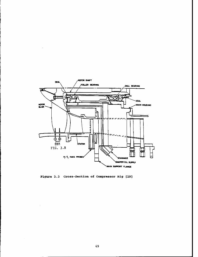
A cross section of the rig is shown in Fig. 3.3. The rotor-
tip diameter is constant at 17 inches. The configuration used no
inlet guide vanes. The rotor shaft is mounted on an oil-damped
roller bearing at the forward location and a ball bearing at the
aft location. The rotors were machined from single forgings3 of
6A1-4V titanium. The stator was also fabricated as an integral
ring machined from AMS 5616. The backward swept stator design
used a controlled diffusion airfoil (CDA) approach for
controlling suction surface diffusion to prevent boundary layer
separation. Stator design parameters are summarized in Table
3.2.
3.2.2 Rotor Designs Tested
Rotors 4 and 6 of the PBS series we:a investigated for the
current stall precursor research. Table 3.2 provides some of the
design features of the rotors. Both are considered low-aspect
ratio, high-throughflow, transonic designs. At design
conditions, rotor tip speed is 1500 ft/s, and approximately 60
percent of the blade span sees supersonic relative flow
velocities. The leading edge of Rotor 6 is swept backwards to
reduce shock losses. Rotor 4 has a more conventional straight
3These single castings are commonly referred to as blisks for bladed disks, or IBRs for integrally bladed rotors.
38

leading edge. Photographs of the rotors installed in the rig are
shown in Figs. 3.4 and 3.5. The location of the high-response
pressure transducers (Kulites) relative to the leading edge tip
of each rotor is also indicated. Close-ups of this area (Figs.
3.6 and 3.7) reveal that the distance from the blade tips to the
Kulites was the same for both rotors, 2.5 inches.
Tip clearance as a function of rotor speed for Rotors 4 and
6 is shown in Fig. 3.8. Note that the clearances are nearly
identical for both designs. Hot (rotating) clearance was
measured with an active, nontouching, spark-gap type clearance
system at the rotor leading edge and mid-chord regions (encircled
areas 1 and 2, respectively, in Fig. 3.3) at two circumferential
locations. The average clearance at design speed was about 0.02 0
to 0.025 inch, approximately 0..6 percent of the rotor tip chord.
Since both sensor location and tip clearances were virtually
identical for both designs, these were not considered as possible
explanations for any measured differences in stalling behavior
between the two rotors.
3.3 Instrumentation
Certain steady-state compressor and facility instrumentation
is considered standard for all tests conducted in the CARL.
These were used for the current tests and will be described
39

briefly in this section. More detail is provided by Law and
Puterbaugh [29]. The main focus of this section is on the high-
response static pressure transducers used for stall precursor
detection.
3.3.1 Test Facility Instrumentation
Rotor speed was measured by a Bentley Model 3 06 proximity
transducer which senses six grooves machined into the
gearbox/rotor driveshaft coupling. The output was conditioned
and directly recorded by the data acquisition system (DAS). A
tachometer provided visual indication of rotor speed accurate to
about 10 rpm.
Inlet mass flow was metered through a 3 0-inch venturi (see
Fig. 3.2) with a 17.4-inch throat. Meter accuracy has been
calibrated to ±0.5 percent by the manufacturer (B.I.F.
Industries).
Inlet total pressure and temperature w e measured just
downstream of the last screen in the plenum (see Fig. 3.2).
Because of the low-plenum velocities, compressor inlet total
pressure was assumed equal to plenum static pressure measured by
four static pressure taps manifolded into two pressure sources.
At maximum flow rate, the error is no worse than 0.003 psi
verified by calibration. Total temperature was averaged from
40

nine bare junction thermocouples located in the same axial plane
as the pressure taps at three different radii. Additionally,
relative humidity was measured in the inlet for every steady-
state test point and subsequently treated in the data processing
software for the calculation of mass flow rate.
3.3.2 Compressor Instrumentation
Compressor steady-state instrumentation is shown
schematically in Fig. 3.9. A total of 276 sensors were used to
measure aerodynamic parameters at various locations throughout
the stage. Nine thermocouples were mounted in the stator vane
leading edges and 80 were located in 10 discharge plane rakes.
The thermocouples are of the slot vented type shown in Fig. 3.10.
A total of 125 pressures were measured in the flowpath;
3 6 static pressures and 89 total pressures. Casing static
pressures were made at 15 axial locations, 12 of these over the
rotor tip (see Fig. 3.9). The total pressure probes were all
Kiel stagnation tube design (Fig. 3.10) and were divided in a
manner identical to the thermocouples. Both discharge plane
total pressure and temperature rakes were uniformly distributed
around the circumference and spaced to divide a single exit vane
passage into 10 equal parts.
41

The only compressor measurements used for the current
analysis were the total pressures and temperatures measured by
the discharge rakes (Fig. 3.9). These were averaged and used
with the inlet measurements in the computation of stage pressure
ratio and adiabatic efficiency for each steady-state data point
acquired during the test program (discussed in Section 4, Figs.
4.1 and 4.2).
3.3.3 Calibration and Measurement Uncertainty
Since the main concern of the present work is the analysis
of unsteady pressure signals, the steady-state pressure and
temperature calibrations will not be discussed here. Details of
the calibrations are provided by Law and Puterbaugh [29]. The
steady-state measurements were used in the current research to
define where precisely on the fan performance map the first signs
of pre-stall behavior occur. Table 3.3 indicates the accuracy to
which this could be done. The uncertainties reported in Table
3.3 were determined through a combination of measurement device
performance specifications (for bias error) and facility
historical performance (for precision error). Each measured
value (pressure, temperature, etc.) was perturbed slightly to
obtain the performance sensitivities to changes in various
parameters.
42

3.3.4 Data Acquisition System (DAS)
Fan rig performance and calibration data were collected by
the DAS. The DAS consists of a MODCOMP MODACS digital and analog
I/O subsystem, a MODCOMP ATC communications I/O subsystem, and a
high-frequency analog data recording subsystem, all controlled by
a host computer. The host computer is a MODCOMP Classic 11/15
16-bit microprocessor with 512 kilobytes of memory and additional
peripherals. Additional information can be found in the report
by Law and Puterbaugh [29] .
Facility and rig controls and compressor operating
parameters are all patched to a control room for monitoring
during testing. A photograph of the CARL control room is
provided in Fig. 3.11. The DAS software capabilities include
real-time update of compressor performance parameters, automated
data recording, and DAS health monitoring.
3.3.5 Unsteady Pressure Measurement
Eight high-response static pressure transducers (Kulite
model XCEW-1-187-100 G) were located in the compressor inlet for
detection of unsteady pressure perturbations. Table 3.4
summarizes the performance characteristics of the transducers.
The transducers were equally spaced around the circumference
43

casing approximately 0.3 rotor radii (2.5 inches) upstream of the
rotor tips (exact locations for each rotor shown in Figs. 3.6 and
3.7). Actual circumferential location of each transducer is
indicated in Fig. 3.12. As noted in the Appendix, the equal
spacing around the annulus simplifies the Fourier analysis that
is useful in determining the presence of modal waves.
Since the present work was concerned with unsteady pressure
signals, the Kulites were operated in a differential mode. The
reference side of each transducer was manifolded to a static
pressure tap located at approximately the same measurement plane
as the Kulites. A long tube length was used to effectively
filter any unsteadiness from the reference side. Thus, measured
signals were true unsteady pressure perturbations.
The path of each of the Kulite signals is shown in Fig.
3.12. A B&F model input conditioner provided 15-volt excitation
and completed the electronic bridge. Variable gain amplifiers
(Bell and Howell, and Neff) were adjusted to allow for maximum
sensitivity without driving the background noise levels too high.
The signals of interest were expected to be on the order of one-
tenth of a psi, thus it was desirable to keep the background
noise below this level. After amplification, the signals were
analog recorded (FM on 100-kHz carrier) on a 14-channel Bell and
Howell model VR-3700B recorder and patched to oscilloscopes for
44

on-line monitoring. A spectrum analyzer was also available for
on-line use. All data processing was performed post-test, and is
described in the next chapter.
In-place calibration of the Kulites was accomplished using a
Druck DPI 510 pressure controller/calibrator, sequentially
applying the calibration pressure to each transducer. Amplifier
gains were adjusted (resulting gains were about 200) so that 5.0
psig provided a 2.0-volt dc transducer output. Static (non-
rotating) noise levels with these amplification settings were no
greater than 10 mV peak-to-peak for each of the eight channels.
Each transducer was calibrated with 5.0, 2.0, 1.0, 0.5, 0.2,
and 0.1 psig control pressures. The calibration data is
summarized in Table 3.5. An important consideration from the
calibration process was that any signal less than approximately
0.1 psi would be lost in the noise. All the calibration curves
were linear down to about 0.5 psig. In fact, only Kulites 2, 3,
and 5 displayed significant nonlinearities (see Table 3.5) at the
very low pressures (<0.5 psig). Despite the nonlinearities of
the three transducers, linear calibration curves (all with a
slope of 2.5) were applied to each Kulite signal for the
following reasons:
(1) The unfiltered measured pressures all contained high-
amplitude, high-frequency components (i.e., blade passing
45

frequency) that placed the Kulites in their linear operating
range over most of the low-frequency period of interest (the
fundamental frequency of interest is approximately 5 0 percent of
the rotor frequency).
(2) The prime concern is frequency content rather than
exact amplitude definition.
46

0 u « u 0
« J
A u u IB 0 a at «
■0 0 M 0 < M 0 a to o u I o u
o »4
g •H
E
47

•HEAT EXCHANGER
HJWJUUUJ CONE
INLET DUCT
TUKWNOU KRKMTEOCONE
TtMNtNO WNC5 COLLECTOR
Figure 3.2 Schematic of 2000-HP Test Facility
48
SEM..
\
/ROTOR SHAFT
.ROLLER BEARING BALL BEARING
SEE FIG. 3.8
SCAVANGE
OAMPER OIL SUPPLY
MAIN SUPPORT FLANGE
Figure 3.3 Cross-Section of Compressor Rig [29]
49

Figure 3.4 Rotor 4 Installed
50

Figure 3.5 Rotor 6 Installed
51

a o
•H V * Ü O J
4>
0) G
•H s o
CO
M 0 W 0 Pi
<W 0
B I 0 a 0 H U
PI
o U
g •rl fa
52

ü 0 ■H
10 U 0
0 43
3 c
•H
I XI W
n 0 *J 0 PS
<H 0
& I 0 n o H u
o
4)
g
53

0.05
10 15 ROTOR RPM 1x10001
20
0.05r-
ROTOR RPM 1x1000)
Figure 3.8 Rotor Tip Clearances
54

Total Praaautaa and Tamoarawai:
StagaExtt
PI/Tton»faX«-,
COMPRESSOR INLET MEASUREMENTS • VarMun inlat Praaaura (4) • VankiA Throal Praaaura(12) - Ralatva HuMe% (1) • Planun Praaaura (2) ■ Planun Tamparaiura (9) ■ Aanoaonartc Praaaufa M*|
Gaming stage Praaaurat:
Figure 3.9 Compressor Instrumentation
55

VANE LEADING EDGE TOTAL TEMPERATURE
D "
VANE LEADING EDGE TOTAL PRESSURE
DISCHARGE-PLANE TOTAL TEMPERATURE
p-n-iuuuin
DISCHARGE-PLANE TOTAL PRESSURE
JUU^JUUlJUl
Figure 3.10 Vane Leading Edge and Discharge Plane Rake Instrumentation [29]
56

g 0 0 es
0 u u a o u
c
g •H
57

k_
CD — C
CO o c -zz .S>=5 CO c o
O
E CD N
•♦■* >» o CD CO Q.
CO c <
CD Q.
CD O Q. O & to 1— O D) — o O
(/) CO c O < ■o
c CO
A v a tu
& ■H CO
■d c A)
o •H 4J «I U 0 a o 4J
ä
o n &
•H
58

Table 3.1 Facility Operating Parameters
Speed Range
Flow Range
Rotor Tip Diameter
Inlet Total Pressure
Steady-State Pressures
High Frequency Pressures
Dynamic Strain
Rotor Tip Clearance
6000 - 21,500 rpm
20 - 60 lbm/sec
14 - 19 inches
6-15 psia
160 + channels
12 channels
10 channels rotating
20 channels stationary
8 channels
59

Table 3.2 Rotor/Stator Design Features1
Design Speed
# of Stages
IGVs
Tip Radius2
Hub Radius2
Mean Radius2
Rotor/Stator Gap
20,222 rpm
1
None
8.50
2.65
5.58
0.88 tip; 0.29 hub
* Bladoa Mid-Chord Caabax* •tanar* Tw±»t* Solidity1 Aapaet
Ratio*
Rotor 4 20 3.95 12.98 44.62 46.86 2.20 1.32
Rotor 6 20 4.34 11.97 30.10 41.85 2.28 1.25
Stator 31 2.25 45.30 14.75 4.86 1.78 1.25
Notes: 1. 2. 3. 4. 5.
All dimensions in inches and degrees At leading edge At mean radius Twist defined as tip stagger - hub stagger Aspect Ratio defined as mean span divided by the average of chord at hub, mean, and tip
rotor stagger stator
stagger
amber
60

Table 3.3 Steady-State uncertainty Analysis
%N„
40
80
100
a. Mass Flow Calculation Uncertainty
Parameter
Magnitude
(lbm/s)
22.611
49.309
61.913
Uncertainty: 95% CI
± Actual
0.339
0.264
0.260
± % Read
1.500
0.536
0.420
Uncertainty: 99% CI
± Actual
0.474
0.373
0.366
± % Read
2.095
0.756
0.591
b. Pressure Ratio Calculation Uncertainty
%NC Parameter
Magnitude
Uncertainty: 95% CI Uncertainty: 99% CI
± Actual ± % Read ± Actual ± % Read
40 1.122 0.005 0.404 0.005 0.490
80 1.580 0.001 0.063 0.002 0.127
100 1.921 0.001 0.077 0.003 0.161
61

Table 3.4 Kulite Performance Characteristics
Rated Pressure
Maximum Pressure
Operational Mode
Excitation Voltage
Maximum Excitation
Sensitivity-
Zero Pressure Output
Temperature Range
100 psig
200 psig
Differential
15 Vdc
2 0 Vdc
1.5 0 mV/psi
< ± 5% Full Scale
-40 °F to 500 °F
Table 3 . 5 Kulite Calibration Data
Input
Press.
(psig)
Output Voltage (V)
Kulite #
1 2 3 4 5 6 7 8
5.0 2.000 2.000 2.000 2.000 2.000 2.000 2.000 2.000
2.0 0.796 0.783 0.770 0.796 0.851 0.806 0.800 0.791
1.0 0.396 0.376 0.359 0.396 0.458 0.409 0.403 0.386
0.5 0.195 0.174 0.155 0.200 0.270 0.208 0.203 0.186
0.2 0.075 0.053 0.032 0.080 0.150 0.089 0.085 0.067
0.1 0.032 0.013 0.013 0.040 0.111 0.049 0.044 0.026
62

4.0 TEST PROCEDURE AND DATA PROCESSING OF UNSTEADY PRESSURES
4.1 Test Procedure
All of the Kulite data were obtained at both steady-state
and transient operating conditions at five different speeds (60,
70, 80, 90, and 100 percent design speed) for each rotor. For
both rotors, a detailed steady-state performance map was
generated prior to the acquisition of any unsteady pressures.
The maps, shown in Figs. 4.1 (unswept, Rotor 4) and 4.2 (backward
swept, Rotor 6), were used for determining throttle settings for
starting the transients to stall and for the near-stall steady
operating conditions.
The steady-state data were obtained very systematically.
Upon reaching a desired speed, a 3-minute settling time was used
to allow system transients and thermals to steady out. After
this, a throttle position was set and another 2 minutes of
settling time was used before acquiring 30 seconds of Kulite
data. The procedure was repeated for each change in throttle
position and compressor speed.
Only one throttle closure rate was available for obtaining
the compressor transient data to stall. At each speed, the
throttle was initially set so that the compressor was at some
nominal unchoked operating condition (about 7.0 percent greater
63

flow than that at the near-stall steady-state condition). The FM
recording tape was then turned on and Kulite data recorded while
the throttle was continuously closed. Once stall was detected
(both audibly and by monitoring the Kulites), the surge valve was
immediately opened and the stall was cleared. A typical throttle
closure to stall (transient) took between 13 and 15 seconds. The
throttle closure rate was approximately -0.3 lbm/s/s, calculated
as defined below:
dW = Ws,a„ - Wini,ia, ., Q3lbm/S (4 1}
dt At ' s
During the transients, it was observed that the compressor
stalled at a lower mass flow than the steady-state stall point
(the indicated throttle position was about 5 percent more closed
during transient stall). This was not unexpected given the
rather fast closure rate (compare Eqn. 4.1 with the rates used by
Gamier [28] discussed in Section 2.4) and the well-known fact
that most separation phenomena seem to have a time constant
associated with them. Figure 4.3 schematically demonstrates the
transient behavior of both an isolated airfoil and compressor.
This unsteady flow behavior helps explain why rotating
disturbances could be detected prior to stall during the
transients, but were not discernible in the majority of steady-
state points (discussed in Section 5.0). Unfortunately, other
64

than the inlet Kulites, no transient measurements were available
for the test programs. Consequently, accurate location of the
transient stall line could not be determined.
4.2 Data Sampling
As noted previously, all unsteady pressure signals were
recorded on analog tape and postprocessed after the testing was
complete. The tapes were played back on a Honeywell model
Ninety-Six Magnetic Tape System and all signals were low-pass
filtered using a Rockland Multichannel Filter System 816. The
filtering was used to prevent massive file storage problems, and
because the maximum frequencies of interest were expected to be
approximately 600-700 Hz (the third harmonic of 50 percent of the
rotor frequency, the fundamental frequency of interest).
Consequently, an 8-pole Butterworth low-pass filter with a cutoff
frequency, fc, of 1 kHz was configured. Filter characteristics
are shown in Fig. 4.4. Also, since the concern was on the
pressure perturbations, any dc-bias was removed from the signals.
Taking the sampling theorem (accurate reproduction of an
analog signal requires sampling greater than twice the highest
frequency of interest, Stearns and Hush [33]) and filter
characteristics (Fig. 4.4) into account, the signals were sampled
at a rate of 4 kHz. Note that a 4 kHz sample rate places the
65

Nyquist frequency (one-half the sample rate) of 2 kHz at twice
the filter cutoff frequency, 2 fc. Any signal greater than 2 kHz
and sampled at 4 kHz has the potential to be artifically
introduced as a lower frequency (aliasing); however, according to
Fig. 4.4, a frequency at 2 fc is down in amplitude by 48 dB.
Thus, the 4 kHz sample rate was chosen as a good tradeoff. between
controlling file size and minimizing any aliasing. Examination
of the spectrums of the unfiltered and filtered signals revealed
that no aliasing occurred. Thus, with 8 channels digitized at 4
kHz, sampling a 10-second record resulted in a 2.56-Mbyte data
file (8 bytes per sample per channel). All data were stored in
standard ASCII format with each column containing the sampled
filtered signal from one of the eight Kulites.
4.3 Additional Digital Filtering
In addition to the analog filtering, unwanted frequencies
were removed by using digital finite impulse response (FIR)
filters. These were chosen for their desirable characteristic of
linear phase shift (constant time delay).
Upon examination of the raw analog filtered traces and
spectrums of those traces, it was found that several unwanted
frequencies were present from many different sources. All traces
showed a 1/rev rotating wave (i.e., at the rotor frequency) and a
66

very strong low-frequency planar wave (and several harmonics).
Several channels had strong 60 Hz (and harmonics) electrical
noise components. Figure 4.5 shows an example of a frequency
spectrum that was obtained from Kulite #2 at 90 percent speed
(310 Hz). All of the just-mentioned frequencies are evident in
the spectrum. The planar wave with fundamental frequency at
approximately 13.5 Hz is believed to be a system resonance. It
had a significant effect on the results and is discussed further
in the next chapter.
Among the many alternatives for handling the unwanted
frequencies, it was decided to digitally band-pass filter the
data around the rotating stall frequency. This limited the
examination of the modal waves to the first harmonic (SFC #1),
but was done for the following reasons:
(1) It was the simplest means for removing the majority of
the unwanted frequencies.
(2) Examination of the first three rotating modes (via
Fourier techniques discussed in Section 4.4.2) revealed that most
of the modal wave energy was contained in the first harmonic and
the additional filtering enhanced its features.
(3) The frequency of the first harmonic for all speeds was
approximately 50 percent of rotor frequency (the rotating stall
67

frequency). Consequently, the second modal wave harmonic showed
around the 1/rev frequency making it difficult to resolve.
Shown in Fig. 4.6 is the same trace as in Fig. 4.5, but
band-pass filtered between 13 0 Hz and 23 0 Hz. Comparison of the
two figures reveals no attenuation of the frequencies in the
range of interest. Additionally, no new information has been
introduced as a result of the filtering. The before and after
spectra of each filter application were checked in this manner to
ensure no erroneous results were introduced. Table 4.1 contains
a summary of the frequency band-pass applied to the data at each
compressor speed. In each case, a 248-order, Hamming-windowed,
FIR filter was applied using MATLAB [30] tools. Unless otherwise
indicated, all plots presented in the next chapter were generated
from the band-pass filtered data with frequency range given in
Table 4.1.
4.4 Forms of Data Presentation
Three basic forms of data presentation were used to aid in
the analysis of the measured unsteady pressures. These included
plots of the filtered raw traces, magnitude and phase of spatial
Fourier coefficients (SFCs), and power spectral densities (PSDs)
of the SFCs. Figure 4.7 summarizes the signal processing
techniques used for characterizing the stalling process. MATLAB
68

[3 0] was the software package used for the signal processing and
plot generation. Each form provided valuable information as is
seen in the next chapter. The details of each are provided
below.
4.4.1 Filtered Raw Pressure Signals
Prior to any Fourier analysis, the filtered raw pressure
signals were examined extensively. In particular, the last
20-100 rotor revolutions (rotor revs) prior to stall were
carefully studied for any evidence of a stall precursor.
Calibration curves were applied to all pressure signals so that
plots of the filtered data traces reveal actual pressure
perturbations in psi (rather than volts). Figure 4.8 is an
example of a raw signal plot which clearly indicates the presence
of a rotating disturbance. The traces were artificially
separated to help view the individual signals (otherwise they
would lay on top of each other) and track the rotating phenomena.
In all the plots which display the eight individual signals,
Kulite #1 (see Fig. 3.12) provides the bottom trace and Kulite #8
the top trace.
4.4.2 Spatial Fourier Coefficients
69

The pressure signals were spatially resolved through the use
of the discrete Fourier transform (DFT). A review of Fourier
techniques with application to the current work is provided in
the Appendix. By taking the period to be eight, the SFCs can be
computed at each discrete time from:
Ck = -2^P(Qn,t)e~r (4.2)
where k is the mode number, or wave harmonic. As discussed in
the Appendix, the ck' s are complex conjugates, but for the case
of eight equally spaced measurements, only the c.k of the first 3
modes (c_i, c2, c.3) need be computed. Thus, it is seen from Eqn.
(4.2) that eight pressure traces are reduced to a single complex
number at each instant in time. The complex number (SFC)
contains the desired phase and amplitude information for each
spatial wave number, k, which can then be tracked in time.
If:
ck = x+jy (4.3)
Then:
X
If a sinusoid is present, the phase, _ck, represents the angular
position of its peak.
70

Plotting the amplitude and phase of each SFC as functions of
time helps reveal any rotating perturbations that might be
present in the system. Of these, the unwrapped phase plots4 can
be the most revealing as a rotating disturbance propagating at a
constant speed will show up as a constant slope. However, care
must be taken in interpreting these plots as the _ck will "lock
on" to the most dominant rotating disturbance.
Figure 4.9 illustrates the usefulness and potential pitfalls
of applying the spatial DFT. The plots show 7 0 rotor revs up to
and including the start of a rotating stall at 90 percent speed
(stall at t=464). Both phase plots indicate the presence of a
rotating disturbance. However, calculations of the slopes reveal
that in Fig. 4.9a, the disturbance is propagating at the rotor
frequency (l/rev=310 Hz). This is further evidenced by the
change in slope at approximately t=461 when the rotating stall
frequency dominates. In Fig 4.9b, the undesired rotor frequency
has been removed prior to performing the DFT, and the phase plot
now reveals the desired rotating stall frequency prior to stall
(no change in slope at t=461). It is also of interest to compare
the amplitude plots of both cases. Note that the 1/rev
4Phase plots are typically confined between n and -%. For the case of a rotating disturbance, it is convenient to unwrap the phase and allow it to grow with time.
71

disturbance is the major contributor to the amplitude prior to
the actual stall as evidenced by the reduced magnitude plot (Fig.
4.9b) after the 1/rev component is removed.
4.4.3 Power Spectral Densities
By performing a temporal Fourier transform or standard fast
Fourier transform (FFT) on each SFC, the power spectral density
(PSD) of an SFC can be computed. Examination of the PSDs can
reveal pre-stall waves that otherwise would be masked by other
rotating phenomena, for example, a strong 1/rev signal. Figure
4.10 is an example of a PSD taken on the same data used to
generate Fig. 4.9a (but not including the stall itself). Note
that in addition to the expected strong peak at 1/rev, a peak is
revealed at approximately 50 percent rotor frequency. No
evidence of this frequency was apparent in the phase plot of Fig.
4.9a.
When computing the spectrum, only data up to the stall event
must be used. If any of the in-stall data is included, the stall
will dominate the spectrum and no conclusions will be able to be
made regarding the small amplitude pre-stall behavior. To
alleviate this problem, PSDs were performed on the near-stall
steady-state data (as close to stall as possible without
inadvertently dropping into stall) and the portion of the
72

transient data up to (but not including) stall. Also, as
described in the Appendix, because the SFCs are complex numbers,
the PSDs are not necessarily symmetric about zero frequency.
Only those PSD peaks which do not exist at identical positive and
negative frequencies indicate rotating disturbances. Thus, both
the positive and negative frequencies were overplotted.
73

102.0-1
100.5-
> ü
jjj w.oH ü
S 97.5H ü
< O
2 94-H g CO
S 93-<H
91.5-
90.0-
105.0-j
100.0-
95.0-
< OC 90.0H LU er D CO CO UJ OC Q. z C3
85.0-
80.0-
23 75.0-]
70.0-
65.0-
60.0-
90Z 1002
80Z
□
n □
60Z
O
70Z
a
□ a
a a
40.0 50.0 60.0 70.0 80.0 90.0
% DESIGN FLOW RATE
100.0 110.0
100Z
90Z
□no °am, 80Z
noocftBn 70Z
60Z design corrected speed
40.0 50.0 60.0 70.0 80.0 90.0 100.0 110.0
% DESIGN FLOW RATE
Figure 4.1 Steady-State Map of Rotor 4
74

IUü.U—
100.5-
> 902
ü O z 111
99.0-
ü LL LL UJ
97.5- 80Z
e O 1- 702 □ □ < m 96.0-
602 □ □
< Q □ 8 o < Z 94.5- □ o CD □ a W 8 a
a if
UJ Q 93.0- a □ s? a a □ □ a □ □
91.5- a □
a
9U.U i i i i i 40.0
c r
105.0-]
100.0-
95.0-
90.0- UJ QC
W 85.0- CO UJ a: a. 80.(H z g 05 75.0- Q
* 70.0-
65.0-
60.0-
50.0 60.0 70.0 80.0 90.0
% DESIGN FLOW RATE
[rpCCD
L00Z
n a
100.0 110.0
1002
902
802
702
SUQ 602 design corrected speed
40.0 50.0 60.0 70.0 80.0 90.0 100.0 110.0
% DESIGN FLOW RATE
Figure 4.2 Steady-State Map of Rotor 6
75

Lift
^ transient
steady-state
Angle of attack
Figure 4.3a Transient Behavior of an Isolated Airfoil
Pressure
ratio
y
transient . ^ N
stall line ^ i^ » s' /\ ^steady-state
stall line
Mass flow rate
Figure 4.3b Transient Behavior of a Compressor Stage
76

.Jfc o'
-100
NORMALIZED FREQUENCY fc I
2fc 3fc 4fc 5fc I ill
L25fc L5fc l.75fc 2fc
120«
24C
360"
480"
600»
720» lOfc
Figure 4.4 characteristics of Butterworth Analog Filter
77

Spectrum of Kulite #2 - 90% speed
Figure 4.5 Spectrum from Kulite #2 - No Additional Filtering
Spectrum of Kulite 12 (filtered) - 90% speed
350
Figure 4.6 Spectrum from Kulite # 2 - Band-Pass Filtered
78

<D 00
Zt CD ** en <n • MM
CO 3 CO *
ß 0
•H JJ (0 N
•rl H fl> *J 0 (0 H a o c 0
■H •U
» O a H
01
H 0
M-t
•0 O « D a o a >t
d
o u
g •H
79

o o in
03 en "3*
P3 en <Ti > *r tu
u u
o 0 a\ ■p *r o
u
00 <D CO s ** •H
oc
~i 00
00
o 00
I
I a
•H V
w o PS
(X ß
•H
§ CO
a o « n
V VI 3
P4
00
o M
s •H fa
Q,$H<UWW3H<D M^3^0^.H0C!(1 v^aw.H^
80

Digital hiqhpass filter only
400 410 420 430 440 450
Time (rotor revs)
460 470
2500 400 410 420 430 440
Time (rotor revs)
450 460 470
a. Digital Highpass Filter
S 0.4 F C
0.3
0.2 -
M a 9 n i t u 0.1 h d e
l/rev-310 Hz
400
800
410 420 430 440 450
Time (rotor revs)
460 470
400 410 420 430 440 450 460 470
Time (rotor revs)
b. Digital Bandpass Filer
Figure 4.9 Illustration of SFC #1 Analysis - 90% Speed Transient
81

01
u c 01 3 <r 01 u
O
c •H
5-1 CD 4J iH •H 4-1
O C
tsl
m... II > 0) M \ H i
si
u c CD 3 cr 0) M Ct4
4J c 0
•H n C R) H
•0 c c o, to
o\° O
U h to
C 0
■4-1 0
Q to ft
0 u & Eh
cn a CD ü +J u to Swcflc-rtjjs'oaj
82

Table 4.1 Frequency Range of Band-Pass Filters
% SPEED FREQUENCY BAND-PASS (Hz)
60 60-180
70 60-220
80 125-230
90 130-230
100 130-230
83
5.0 RESULTS AND DISCUSSION
5.1 Introductory Remarks
Presentation of results is provided primarily in Sections
5.3 and 5.4 along with some discussion. Because of their effect
on the results, the low-frequency planar oscillations mentioned
in Section 4.3 are discussed first in the next section.
Additional discussions regarding the effects of compressor
speedline characteristic and shock waves are presented in
Sections 5.5 and 5.6. In the last section, results are compared
with those from previous investigations.
5.2 Low-Frequency Planar Oscillations
As noted in Section 4.3, planar waves with fundamental
frequency of about 13.5 Hz were evident in all transient and
near-stall steady data obtained on both rotors. As exemplified
in iig. 4.5, the second harmonic of this wave (27 Hz) was
dominant at all rotor speeds except 100 percent speed for both
designs. At 100 percent speed, the fundamental frequency
dominated. Although the precise nature of the planar
oscillations could not be determined (these type oscillations
were observed in previous investigations; see Greitzer [31]),
they are believed to be the result of some overall system
resonance (rig and facility) for the following reasons:
(1) the frequency did not change with compressor speed.
84

(2) the waves were seen in the near-stall steady-state
data, eliminating the notion that they might be induced by the
throttle ramp rate.
(3) the facility is closed-loop and believed to be more
susceptible to resonances than an open-loop facility.
In order to verify the system resonance theory, the
compressor and inlet and exit ducting were modeled as a Helmholtz
resonator in a manner similar to Emmons, et al. [21] and Greitzer
[31]. The Helmholtz frequency, CO, is defined as:
CO = a M^- • (5.1) \VpLc
where Ac and Lc are the area and length of the equivalent
compressor with constant area inlet duct, Vp is the discharge
plenum volume, and a is the speed of sound. For the current set
of tests, the discharge volume was fixed and the throttle choked;
V was calculated with a high degree of confidence. However,
choosing Ac and Lc were somewhat arbitrary, especially with a
closed-loop facility. Two attempts were made, first including
inlet volume only up to the screens in the inlet plenum (see Fig.
3.2), then adding the remaining inlet plenum volume up to the
perforated cone (Fig. 3.2). The first attempt produced an CO
=149 Hz, the second, CO =80 Hz. The question as to which inlet
volume should or should not be included is undecided, and
85

certainly by including enough, a 13.5-Hz (or 27-Hz) resonator
could be established.
The presence of the planar oscillations complicated the
signal processing procedures used for detection of the rotating
phenomena of interest here. This complication arises because the
oscillations were observed close to the onset of stall and were
consistently detected before any rotating perturbations were
observed (i.e., planar waves could be seen in the near-stall
steady data, rotating waves were not) .
As seen in Fig. 5.1a, the planar waves were initially of
small amplitude and grew as the machine was continually throttled
to stall. Even when the data were high-pass filtered above
60 Hz, the effect of the waves was clear (Fig. 5.1b); the
oscillations effectively throttled the stage into and out of
stall. A clearer picture of this is provided by Fig. 5.2, which
shows the in-stall behavior at 80 percent speed. The behavior
shown is quite consistent with surge-like oscillations (Greitzer
[31]). Of particular interest to the current work is the small-
amplitude "surging" that occurred prior to stall and its
influence on the rotating disturbances. This influence is shown
schematically in Fig. 5.3 and is evidenced in the majority of the
results presented in the next section.
86

5.3 Analysis of Results
Because the rotors studied are so close in design, it is
appropriate to present results via speedline (for both rotors)
rather than by rotor. This allows for direct comparison between
designs and facilitates a discussion regarding any significant
differences in stalling behavior. Signal processing of the data
was performed as described in Section 4.0. Some examples of
signal traces without the additional filtering (Table 4.1) are
also provided. Plots presented as functions of time use rotor
revolutions (rotor revs) as the time scale since this is the
scale of the phenomena of interest. In most time plots, only the
last 1-2 seconds prior to the stall event are shown since the
current investigation is concerned with stall inception.
Rotating stall frequencies for all cases were between 50-56
percent of rotor frequency. A single-stall cell was identified
in all the cases examined. As noted in Section 1.2, both
progressive and abrupt rotating stall were observed. Progressive
stall was seen at low-speed operation (60 percent speed for the
unswept rotor, #4, and 60 and 70 percent speed for the swept
rotor, #6), as would be expected (Greitzer [12]).
At all speeds for both rotors, stall was preceded by small
amplitude rotating waves which grew rapidly once the onset of the
instability was reached. Thus, the plots presented for either
87

rotor are meant to be representative of the stall inception
behavior of both designs. The only significant difference was in
the amount of time the modal waves could be detected prior to
stall. The differences in stall warning time will be discussed
qualitatively in this section, and more quantitatively in the
following section (Section 5.4).
The data digitizing system described in Section 4.2 became
inoperative before any steady-state data for Rotor 6 could be
sampled. In this sense, the data analysis was not as complete as
it could have been. However, given the data that were examined
(Rotor 4 steady-state and transient and Rotor 6 transient), a
high level of confidence is placed in the results and conclusions
that follow.
5.3.1 A 60 Percent Design Speed
This was the only speed where the relative rotor flow
velocities were subsonic across the entire span. As noted above,
a progressive rotating stall was observed for both designs at
this speed. The data traces for Rotor 4 (unswept) were
previously presented in Fig. 5.1; the traces for Rotor 6 were
quite similar and are not shown. The progressive nature of the
stall can be seen in Fig. 5.1b as the pressure perturbations
experience a relatively slow growth (compare the traces in Fig.
5.1b to those of Fig. 5.7b). As indicated in Fig. 5.4, initial
signs of the stall became evident at around t=196. Note the
88
small amplitude rotating wave (=0.2 psi peak-to-peak) at
approximately 5 0 percent rotor frequency (0.5/rev) emerging at
t=196 and being attenuated by t=201.
From a stall warning viewpoint, this case of a progressive
stall is relatively uninteresting as one can throttle in and out
of stall without sudden changes in compressor performance.
However, for completeness, the amplitude and phase plots for SFC
#1 are provided in Fig. 5.5 and do indicate the presence of the
rotating disturbance from about t=190 on. Note that traces of
the disturbance can be seen prior to t=190.
Figure 5.6 shows the PSD of SFC #1 at the near-stall steady
condition (DV053) and next higher-flow condition (DV050) for
which data were obtained. The insert identifies the compressor
operating conditions (percent design pressure ratio versus
percent design flow) corresponding to these two throttle
settings. The peak at 110 Hz (about 51 percent of rotor
frequency; see Fig. 5.5 phase plot) at the near-stall condition
provides further evidence of the pre-stall rotating waves. No
discernible peak at 110 Hz is evident at throttle setting DV050;
hence, no rotating wave behavior is apparent. This was the only
speed in which a pre-stall indication was evident in the near-
stall steady-state data.
89

5.3.2 A 70 Percent Design Speed
As evidenced in Fig. 5.7, the stall at 7 0 percent speed for
Rotor 4 was abrupt and relatively clean (the effects of the low-
frequency oscillations were minimal). The planar oscillations
described in Section 5.2 were still present (their effect can be
seen best in Fig. 5.7b through low-frequency modulation of the
rotating stall frequency), but were not as strong. Examination
of the last 20 rotor revs prior to stall (Fig. 5.8) reveals the
stall cell emerging smoothly from small amplitude rotating waves
(at about t=483). Prior to t=483, it is difficult to detect any
coherent rotating disturbance in the raw traces.
Because the Kulite traces were relativ"v clean of unwanted
frequencies, higher order Fourier modes wei lso examined at
this speed. Shown in Fig. 5.9 are the amplitude and phase plots
of the first two spatial modes (SFC #3 contained virtually no
energy). As indicated in the magnitude plot prior to stall
(stall at t=4855) , the energy content of the first two modes is
quite similar, with SFC #1 displaying slightly more activity.
Both phase plots appear to show a reduced slope change at about
t=470 (from 1/rev to =0.52/rev). The slope from t=470 on
corresponds to a rotating disturbance traveling around the
annulus at about 52 percent of the rotor frequency (note the
5For consistency at all speeds, the onset of stall was taken to be when the amplitude of SFC #1 reached 50% of its final value.
90

slope remains the same subsequent to stall onset at t=485),
indicative of the impending stall. Using the phase plot data of
Fig. 5.9, it appears that minimal stall warning time (15 rotor
revs) is provided at this speed for Rotor 4.
Plotting the PSD of the spatial Fourier coefficients
provides another tool for examining the stall inception behavior
of the compressor. The data obtained during the transient to
stall can be used provided the stall event itself is not
included. The power spectra will then reveal any small amplitude
resonances in the system even if they are present only for a
short duration. This was the procedure followed since the
steady-state data provided no insights into the stalling
mechanism.
Shown in Fig. 5.10 are PSDs of SFC #1 at 70 percent speed
obtained using the transient data including stall (5.10a) and up
to stall (5.10b). The same plots are shown for the second mode
in Fig. 5.11. Because the SFCs are complex, their spectra are
not necessarily symmetric (explained in the Appendix and Section
4.0); consequently, positive and negative frequencies are
overplotted. Peaks that exist at identical positive and negative
frequencies indicate a standing wave (note the twin peaks at 120
Hz in Figs. 5.10b and 5.11 which imply an amplitude oscillation
of a standing wave; due, in this case, to electrical noise which
was strongly present on some channels and not evident at all on
others). Thus, only those signals which do not occur at
91

identical peaks indicate rotating disturbances. A further
complication for this particular speed is that the rotating stall
frequency is quite close to the 120 Hz noise frequency.
Nevertheless, the stall frequency did show up to be slightly
higher (123 Hz) in the data which included the stall (Fig.
5.10a). The same is true in Fig. 5.11a for the second harmonic
(246 Hz). Examination of Figs. 5.10b and 5.11b reveals no peaks
at the stall frequency. Given the 12 0 Hz complication and the
complexity added by the low-frequency planar waves, the spectra
offered no additional information regarding the stalling process.
The stall of Rotor 6 (swept) at 7 0 percent speed was quite
different from that of Rotor 4. The behavior of Rotor 6 was
characterized by a progressive stall very similar to that
descr:. oed in Section 5.3.1 for both rotors at 60% speed. The
progressive nature of the stall is represented in the SFC #1
amplitude plot of Fig. 5.12, where one can see a relatively
gradual increase in the energy content. Also, the effects of the
low-frequency planar oscillations are apparent in the amplitude
plot of Fig. 5.12, as can be seen clearly from about t=570 on
(note the modulations at approximately 27 Hz). Comparison with
the SFC #1 amplitude plot in Fig. 5.9 shows that Rotor 4 stalls
quite abruptly relative to the Rotor 6 stall at this speed, and
the effect of the planar oscillations is minimal. Further
evidence of a slowly developing (progressive) stall is provided
in the phase plot of Fig. 5.12, which shows a relatively constant
92

slope (for the entire 2 00 rotor revs plotted) corresponding to a
rotating disturbance at about 0.5/rev. Despite the differences
in the type of rotating stall encountered (abrupt, Rotor 4;
progressive, Rotor 6) by the two designs at 7 0 percent speed, the
basic mechanism of the stall development process of the two
rotors was identical - growth of small amplitude rotating waves
(Figs. 5.9 and 5.12).
5.3.3 80, 90, and 100 Percent Design Speed
At the higher compressor speeds, abrupt stall (sudden,
discontinuous decrease in performance at stall onset) was
observed for both designs. In this section, the stall inception
process was governed by the growth of small amplitude rotating
waves. Again, the plots presented for either rotor are meant to
be representative of the stall inception behavior of both
designs. It is worth noting that evidence of the upcoming stall
could be seen in the unfiltered (no analog or digital filtering)
raw Kulite signals. At the higher rotational speeds, the
pressure traces were dominated by a strong signal at the blade
passing frequency (believed to be caused by shock waves passing
the Kulites). As stall was approached, the 1/blade signal
started oscillating in both frequency and amplitude,
approximately 1-2 seconds prior to stall onset. This was
observed both on-line while testing and during playback of the
data. This observation is discussed further in Section 5.7.
93

The filtered data traces obtained from the 80 percent speed
transient for Rotor 4 (unswept) are shown in Figs. 5.13 and 5.14.
The longer period indicated between the first two "pulses" of
rotating stall (seen best in Fig. 5.2) was repeatable with the
same rotor and was also seen in the Rotor 6 data at the same
speed. Development of the rotating stall from the small
amplitude modal waves can be seen clearly in Fig. 5.14. Figure
5.15 presents the amplitude and phase data of the first mode and
points out some interesting features. Using the information
presented in Fig. 5.15, there does not appear to be a lot of
warning time prior to the instability as evidenced in both the
magnitude and phase plots. Note the apparent exponential growth
of the rotating waves (from t=464 on) just prior to stall onset.
This is predicted by the stability theory discussed in section
2.3.1 (Garnier [28]). The 1/rev disturbance indicated between
t=423 and 435 is believed to be an anomaly, as the data was
filtered using a 248-pole FIR filter between 125 and 230 Hz.
The spectra obtained using the transient data set (up to,
but not including stall) for Rotor 4 at 80 percent speed is shown
in Fig. 5.16. As evidenced by the lack of any definitive peak,
the PSD does not appear to offer any additional insights into the
process leading up to stall. Several of the peaks (i.e., 150 Hz,
.175 Hz) are believed to be harmonics of the strong low-frequency
planar oscillations (fundamental frequency of 13.5 Hz) evident in
all the data (see Fig. 4.5).
94

The stall behavior at 90 percent speed provided one of the
more interesting comparisons between the two designs. Indeed,
the development of stall from rotating waves for both rotors was
again observed. Figures 5.17 and 5.18 are representative of the
process for both designs. Small amplitude wave growth can be
seen clearly in Fig. 5.18. The most interesting feature of the
stalling process at this speed for both designs was that the
waves were detected much sooner than those for any other speed
examined. Evidence of this is provided in Figs. 5.19 (Rotor 4,
unswept) and 5.2 0 (Rotor 6, swept). Both phase plots show
relatively long periods of constant slope prior to stall,
corresponding to a rotating disturbance at about 50 percent rotor
frequency. Of particular interest are the SFC #1 magnitude and
phase plots for Rotor 6 (Fig. 5.20). Both plots in Fig. 5.20
reveal significant energy contained in the first spatial mode for
at least 260 rotor revs (0.84 s) prior to stall. The reason for
this advanced stall warning time is strongly suggested by
examination of the compressor overall characteristic at 90
percent speed (Fig. 4.2). Note that the 90 percent
characteristics for both rotors (Figs. 4.1 and 4.2) exhibit
positively-sloped regions, with the speedline for Rotor 6 being
most pronounced. The effect of speedline shape on stall
precursor behavior is discussed in more detail in Section 5.5.
The PSD plot of SFC #1 for Rotor 6 (swept) using the
transient data up to stall is shown in Fig. 5.21. As with 80
95

percent speed (Fig. 5.16), the spectra do not reveal any distinct
peaks that might be indicative of small amplitude rotating waves.
The lack of information from Fig. 5.21 does not invalidate the
results just described from the phase plot of Fig. 5.20. Figure
5.21 simply shows that the spectra of the first Fourier mode are
complicated and contain a lot of frequencies (rotating, planar)
of approximately the same magnitude.
At design speed, the stalling process was identical to that
described at the other high speeds - abrupt stall characterized
by growth of small amplitude circumferentially travelling waves.
This is evidenced in Figs. 5.22 through 5.24 for the swept rotor
(Rotor 6). The PSD plots of SFC #1 for Rotor 6 are shown in Fig.
5.25 using 100 percent speed transient data up to stall, and 0.25
and 0.5 seconds prior to stall. A very distinct rotating
disturbance can be seen at approximately 17 0 Hz in all three
plots (Fig. 5.25). Note how the peak attenuates and widens as
data further from the stall were used (Figs. 5.25b and c). This
attenuation suggests that the rotating waves are being damped out
as the compressor moves away from the stall point, consistent
with the stability theory described in Section 2.3.1. Although
not shown, the spectra of SFC #1 for Rotor 4 at design speed were
similar to those shown in Fig. 5.16 and 5.21; no definitive peak
was seen.
96

5.4 Stall Warning Time
In order to arrive at a more quantitative description of the
stall warning time, the following procedure was adopted. The
phase data of SFC #1 were smoothed using a cubic spline smoothing
function (i.e., Fig. 5.26). The choice of the smoothing function
inevitably affects the stall warning time, but as noted below,
the criterion was developed for comparison purposes (the same
order smoothing function was applied to each data set). Since
the slope of the phase plot corresponds to the frequency of a
rotating disturbance, the slope (derivative) of the smoothed data
was calculated and plotted as a function of time up to and
including stall. The stall warning time was then taken to be the
last stretch of slope up to stall that fell between 30-70 percent
rotor frequency (2-4.4 rad/rev). This criterion was developed
merely to provide a consistent means of determining a stall
warning time for comparison purposes. In the plots that follow,
the criterion band and the onset of fully-developed stall are
indicated, as well as the start time taken for stall warning
(arrow).
Plots of the phase slope of SFC #1 for both rotors are shown
in Figs. 5.27-5.34 for 70, 80, 90, and 100 percent design speed.
The 60 percent speed data were not included because of the
previously described progressive stall exhibited at this speed.
The speedline characteristics provided as inserts in each figure
help stimulate discussion in the next section. Emphasis is
97

placed on the shape of the speedlines, hence they are plotted as
percent design pressure ratio versus percent design mass flow
(refer to Figs. 4.1 and 4.2).
Table 5.1 summarizes the stall warning times as calculated
following the above criterion. As can be seen from the plots and
Table 5.1, Rotor 6 consistently provided more stall warning time
than did Rotor 4. With the exception of 90 percent speed (Figs.
5.31 and 5.32), the shape of the speedlines for each rotor were
quite similar. The advanced stall warning times for the swept
rotor (Rotor 6) suggests a potential effect of shock waves on
stall precursor waves, since the leading edge of Rotor 6 was
swept back deliberately to reduce shock wave strength. Shock
wave effects are also discussed later in Section 5.6. In
addition, essentially all of the plots show evidence of the
impending stall 200-300 rotor revs prior to the instability
(i.e., slope within the criterion for a 30-60 rotor rev period
well before the stall, but followed by a significant stretch of
the slope outside the criterion). Very good examples of this can
be seen in Figs. 5.33 and 5.34 at design speed for both rotors.
5.5 Effect of Speedline Characteristic on Stall Precursor
Figures 5.35 and 5.36 show the steady-state performance
characteristics of the two designs as determined using the steady
conditions for which Kulite data were obtained. The high-flow
condition (wide-open throttle) data points are included to
98

provide a better determination of the speedline shape. The low-
flow points at each speed provide a good indication of the
steady-state stall line. Also indicated is a best guess for the
transient stall line (refer to Section 4.1) determined by-
extending the general shape of the speedlines as shown (better
indications of the speedline shapes can be seen in Figs. 4.1 and
4.2). Examination of the extended speedlines offers a potential
explanation as to why the small amplitude waves were not detected
at the near-stall steady conditions, but were detected in the
transients very close to stall. By operating transiently to the
left of the steady stall line, more of the positively sloped
region of the speedlines is reached. It appears that a
positively sloped characteristic (also discussed in Section 2.4)
could be an important consideration for advanced pre-stall
indications.
This hypothesis is further substantiated by examining the
stall warning times (Table 5.1 and Figs. 5.27-5.34) in relation
to the speedline shapes. As seen in Figs. 5.29 and 5.30, the
slope of the 80 percent speedline for both rotors is nearly flat
(maybe slightly positive) and the stall warning time is minimal
compared to the other speeds. In sharp contrast to the 80
percent speedline shape (and all other speeds for that matter) is
the very large region of positively sloped characteristic at 90
percent speed for the swept design (Rotor 6). This condition
provided more than 2.0 seconds of stall warning time. Note that
99

from a design standpoint, operating in a region of large positive
slope is undesirable - performance penalties are large (see for
example the efficiency curve of Rotor 6 at 90 percent speed, Fig.
4.2). However, operating at peak efficiency in a region of flat
or slightly positive slope is desirable (i.e., maximum pressure
rise), and may be beneficial from a stall warning standpoint.
Figure 5.37 is an attempt to provide some quantitative
relationship between speedline slope and stall warning time. The
slopes were calculated by extending a straight line through the
near-stall steady-state data point following the general shape of
the speedline. Results of this rather crude approximation (Fig.
5.37) point out the difficulty encountered in trying to correlate
stall precursor behavior with various compressor parameters.
Another potential problem here is that the statistical data
sample is quite limited (i.e., each rotor was stalled transiently
only once at each speed tested). Since the stalling process has
a lot of random phenomena affecting its behavior, it might be
more appropriate to look at some average behavior for many stalls
repeated at each speed. Additionally, speedline slope is just
one factor. Other important considerations were discussed in
Section 2.4 and include sensor location and sensitivity, throttle
transient rate, flow field distortion, shock waves, and others.
5.6 Effect of Shock Waves on Stall Precursor
100

Figure 5.38 schematically shows the shock structure at
operation close to stall of the transonic rotors tested in the
current experiments. At a high-flow operating condition
(unthrottled), the leading edge shock is attached and oblique to
the inlet relative flow. As the flow is throttled to stall, the
shock becomes more normal to the relative flow and moves upstream
to form a bow shock (Fig. 5.38). Also shown in Fig. 5.38 is the
location of the Kulites used for stall precursor detection in the
current investigation. With this arrangement, the modal waves
rotating at about 0.5 rotor frequency must travel upstream
(decaying exponentially as predicted by theory, Gamier [28]) and
pass through the shock structure rotating at the blade passing
frequency (40 times the modal wave frequency) in order to be
detected. Within this complicated flow field, a quantitative
description regarding the effect of shock waves is difficult;
however, qualitatively, attenuation of the rotating waves would
appear reasonable.
As indicated in Table 5.1, Rotor 6 consistently displayed
more stall warning time than did Rotor 4, even in cases when the
speedline shapes were virtually identical. Figure 5.3 9 shows the
performance characteristics of both rotors on the same map to
provide a good comparison of the speedline shapes. A good
example can seen in the 80 percent speed data for both designs;
Rotor 6 had more than double the warning time of Rotor 4, yet the
speedline shapes were quite similar. In fact, all the
101

characteristics were very similar in shape except at 90 percent
speed. Also, the tip clearances and sensor location for both
designs were essentially the same, as noted in Section 3.2.2.
Thus, it appears that the reduced shock strength of the swept
rotor (Rotor 6) had a positive effect on the ability to detect
the pre-stall waves and supports the discussion in the preceding
paragraph.
Although not the focus of this research, it is also
interesting to note that the swept rotor stalls appeared to be
less severe than the unswept rotor stalls. At 70 percent speed,
Rotor 6 exhibited a progressive stall (Fig. 5.12), while the
Rotor 4 stall was more abrupt (Fig. 5.9). Additionally, the SFC
#1 amplitude plots for the swept rotor showed consistently less
energy in fully-developed stall than did the unswept design (for
example, see Figs. 5.19 and 5.20). The reduced severity of the
Rotor 6 stalls appears to confirm the weakened shock structure of
the swept design.
5.7 Comparison With Previous Investigations
Compressor stall inception for the two rotors examined was
characterized by growth of small amplitude rotating waves. As
measured 0.3 rotor radii upstream at the blade tips, the
perturbations were initially 0.2 psi peak-to-peak. The waves did
not grow significantly until just prior to the instability, when
102

exponential growth into fully-developed stall occurred very
rapidly, typically within 6-10 rotor revolutions.
The features described in the preceding paragraph support
the modal wave representation of the stall inception process,
schematically shown in Fig. 2.3. Results are qualitatively
similar to those obtained from recent experiments on low-speed
compressors (McDougall, et al. [2] and Gamier, et al. [3]) and
one high-speed compressor (Garnier, et al. [3]). Figure 2.4
provides an example of Garnier's, et al. [3] results from a low-
speed machine. The similarities of the results from the current
work (see, for example Figs. 5.19 and 5.20) with the features
shown in Fig. 2.4 are readily apparent. The planar oscillations
evident in the present results were affected when the modal waves
could initially be detected (see Fig. 5.3). Regardless, the
basic mechanism of stall inception was clear - stall evolved
smoothly from small amplitude circumferentially travelling waves.
It is worth mentioning that the high-speed results presented
by Garnier, et al. [3] showed the second harmonic of the rotating
waves (SFC #2) to be at least as important as the first mode.
The present work focused on the first mode for reasons discussed
in Section 4.3 (a lot of unwanted frequencies, most of the energy
appeared to be in SFC #1, etc.). The higher harmonics were
examined only briefly and probably warrant more study. Given
that the rotating stall frequencies of both designs were
approximately 50 percent of rotor frequency, examination of
103

higher order modes would require additional signal processing in
order to resolve the second harmonic and the 1/rev signal. Time
did not allow this additional processing to be performed in the
current investigation.
Finally, another aspect of the stalling process that
deserves some discussion is the high-frequency content that was
filtered out of all the data presented here. As mentioned in
Section 5.3.3, the raw (unfiltered) Kulite signals obtained at 70
percent speed and above were dominated by a very strong (3-4 psi
peak-to-peak) 1/blade frequency generated by the passing shock
waves (see Fig. 5.38). At 60 percent speed, the entire span was
subsonic and the 1/blade frequency was not as evident. It was
observed both on-line and during data playback that during the
transients to stall, the 1/blade signals would start modulating
in both frequency and amplitude (perhaps at 27 Hz). The
modulations could be seen approximately 1-2 seconds prior to
stall and would grow as stall was approached. This observation
raises the question of whether the high-frequency signals due to
shock passing (6.9 kHz at design for the current rotors) might
provide a useful indicator of impending stall, particularly in
high-speed machines.
104

p r e s s u r e
P e r t u r b a t i o n s
{ P 5 i )
a. No Digital Filtering
16 l/rev-204 Hz
14 -
12
10
8k-
0 *-
-2
27 Hz f-
H ■ fc-.. It» « ■ ■> ■OliliuMJMU^fW.
--wA
■.»■■■l.i-l.. w» «**»l^^»^
■—»i*n>-*W» ^w»
.A-^u41v^MU^\MMAM
w i 4» »i.i» »S, i
■ W».«IM.
50 100 150 200 250
Time (rotor revs)
300 350 400
b. Digitally High-Pass Filtered
p r e s s u r e
P e r t u r b a t i o n s
( P s i )
16 l/rev-204 Hz
14
12
10
-2
progressive: stall begins
III K *»» «In II 4i *i r«»i**i4»i|>1 *»ff f
■i" »II -nw»-t>—»ü^«iwvii«-iM«4t. U^.f^ffj * » mnwl) II >nf .U»J» ««^»f ^ ♦^t*
>'■ il .ini da» oiiia»«4l i'i"i*»>i4i.»>li> >4f iti It
i 1 h ' '*» >J< II ii «4 ■, ')»»<>iLJ»4» »'
iih ■.< »■» i.4»*lll»« w«»i^4 »4»l4f f 44
■»■1111*111 rtmi^iuwVwIi »^^IMW^^T^f iUt'4
_i_
50 100 150 200 250
Tine (rotor revs)
300 350 400
Figure 5.1 Low Frequency Planar Oscillations - 60 Speed, Rotor 4
105

o
in
o en in
o
in u 0 a 0
o o o
in to to
> o\° tu o
CD
u
o u 0 4J
o 4J H in 0 u ■a
4J a a <D H
o s •H
0 X
E-t •H
1 (9 ÜI M 3 CD
N
o • 03 in
•«*• • u
•rt
O r» ^
o
CUS-(<1JCQCQ3MC1J D-(l)h4J3hJ2(fl4J-HOCtQ ~ a W -H ~
106

Pressure Ratio
small amplitude rotating
disturbances' detected
^ no rotating disturbances
detected
small amplitude planar oscillations effectively "throttle"
compressor
Flow
Figure 5.3 Hypothetical Behavior of Compressor Durina Transient to Stall with Planar Oscillations
107

o r-i
03 O CN
O
O CN
CN 01 O > CN tu
u u
O 0 o •u CN 0
u
OS <D o\ s
0 ■H u
«I a o
•H 4J •H ■0
a 9 n
a o «
o
if o to
in
ai U
g. •H
cuu<Dviui3u<D a (DM+i 3 ma (8^-HO c ra -^aw-H
108

BE
o
'■IT- >
u
•«* m c>«
o o o
03 EL. U 2 (0 D^C
u 0 *i 0
0 0, m *° © to
u fa n
o « o « Pi
in
in
o U
g •H
ültuU CUÄtCWQ) ^ M (0 >0 ~
109

T3 (D 0) a CO
dP O
Q CO
X
>i o e a) 3 cr a) M
u 0
*
n
*: 0
-s Ü • h •
«4 o #
O QW a
fl-H o *» ■ •H «< ■ u o « 01
10
in
u &
waaüJJMWM Sfocnc-HAj-'oa;
no

? r e s s u r e
P e r t u r b a t i o n s
( P s i
rotating stall (0.52/rev)
300 350 400 450
Time (rotor revs)
500 550
a. No Additional Filtering
p r e s s u r e
P e r t u r b a t i o n s
-1
l/rev-239 Hz
- ^^^^-■■—■J^W «WWOnnw^u^y^MJ^MW—W"*
'+*'*'ll*+*'*+*At*ifi*M*****fitM
««ft*-* ■ ■ »ft i»MIMiHW»'.lll ^V^W^S^
300 350 ♦00 450
Time (rotor revs)
500 550
b. Bandpass Filtered Figure 5.7 Pressure Traces During 70% Speed Transient, Rotor 4
111

o
as 00
00
U 'S" 0 00 u
0 T
• jm* ■
CN CO fi 00 > ^" CD o
U
Sn « o 0 a 03 4J 0 •V 0 a
u • **^ u
a 00 CU
H
r» E H H
■*< •H « fr a
CO
vo • p^
in
TP • u
s TI fa
CN r-
o r-
OtUOUlUlZUV CU0)^^3^Xi(T34J^OCW ^- a co -H ^-
112

o o in
a\ "4*
u o 0 a\ 0 •<? OS
■0 o s a
in DJ 00 <# ^ o
a o 05
0 ■d
CO > £ U •
U U 3
in 0 0 t>» +J h
^ 0 i-4
u *
"** V m
o (0 CO
p* s 'S **• -H a
0 o •
CO
•d in VO 9 *»• V
a M
o 0« • vo in **• •
u &
in in ^«
o in
CO 1X4 U 2(0CiC-H+J3'CII) WfeU b£ « to OJ ^MfO'O^
113

10-* c-..l/rev"7'iq Hy
•a
& CO
100 150
Frequency (Hz)
a. Including Stall
IQ-* l/rev-239 Hz
10-«
Figure 5.10
Frequency (Hz)
b. up to Stall Spectra of SFC #1 Transient Data at
114
70% Speed, Rotor 4

l/rev-239 Hz
■S 3
«0
s 1 8.
CO
100 120 140 160 180 200 220 240 260 280 300
Frequency (Hz)
Including Stall
u 3
10
10-*
, l/rev239 Hz J I- JL J
r:::::QQlB6
10-» ss
10-»
iiiliiilliiiliil^ ^K-im
100 120 140 160 180 200 220 240 260 280 300
Frequency (Hz)
b. up to Stall Figure 5.11 Spectra of SFC #2 Transient Data at 70% Speed, Rotor 4
115

...ffi...
m CN
II
U \
o CN
in
en > cu u
u o 0 © +J in 0
u
o 03 E •*S" •H
EH
O 10 **
o
<N
O
in m o
o o
W fa O 2f0CT»a-H+J3'O(l)
V« 0 4J
« «I Q
U a
n
# o
»4 0
Da
H
in
u s
WCt4(J Q.X! (B WdJ wfnfQrO^
116

p r e s s u r e
p e r t u r b a t i o n s
( P s i. )
l/rev-275 Hz
Oh
100 200 300 400
Tine (rotor revs)
i 11 '
fwif
ffwj# 500 600
Figure 5.13 Pressure Traces - 80% Speed Transient, Rotor 4
p r e s s u r e
P e r t u r b a t i o n s
( P s i )
460 462 464 466 468 470 472 474
Time (rotor revs)
476 478 480
Figure 5.14 Stall Inception at 80% Speed, Rotor 4
117

o 03
o
O
O in
CO >
u u o ■p o u
0) E
X
in r- CN
h-« >
U \
o CN
©
O
en
©
CN
o
o o
o 03
o
o *»« h
0 u
■Ü • o • in *^ B ■«r w jf > o
(U OB
u H u *
o 0 Ü <«• ■p h. ^« 0 a
u <H 0 •
tt) g A
o •H Pi en &H 1
• 3 4J •H H
o 1
o H
O o
10
& ■H h
o CN
W En U 2 (0 OiC-H+J 3<o Q; WCKCJ Q.Ä (0 W a; whflü«
118

u 0 w o tu
s 9 A a # o 00 o
o 1
CN H H
*—* n 1SJ 0 s i>
*-' & o 00 r-1
a a a)
• a M V
3 D tr a a) 4J
S-l s b ■H
a 9
o M H vo
iH 01 0
•H ■
H *
a o <M ** 0 l-l a a
Pi
o
l O H
at I O
10 H • in
M
g ■H h
O
«do) U+J n «H Sf0tnc-H+J3,O(U
119

p r e s s u r e
P e r t u r b a t i o n s
( P s i )
l/rev-310 Hz
Hf +4
-* 44*
+4
+4H 100 200 300
Time (rotor revs)
400 500
Figure 5.17 Pressure Traces During 90% Speed Transient, Rotor 4
P r e s s u r e
P e r t u r b a t i o n s
( P B i )
450 452 454 456 458 460 462 464
Time (rotor revs)
466 468 470
Figure 5.18 Stall Inception at 90% Speed, Rotor 4
120

S 0.4 F C
M °-3 a
n 0.2h i t u 0.1 d e
l/rev-310 Hz
300 320 340 360 380 400
Time (rotor revs)
300 320 340 360 380 400 420
Time (rotor revs)
420 440 460
440 460
Figure 5.19 SFC #1 Amplitude and Phase - 90% Speed, Rotor 4
S F c
H a g n 1 t u d e
S P C
P h a s e
( r a d )
0.4
0.3 -
0.2
0.1
1800
1600 -
1400 -
1200
1000 400
450
450
500 550
Time (rotor revs)
600 650
600 650 500 550
Time (rotor revs)
Figure 5.20 SFC #1 Amplitude and Phase - 90% Speed, Rotor 6
121

o
CN
O U 0 V
n to
o 01 o 1 CN H
H «
^"* 09 N X 0
V N~*
* o >1 4) 00 H
u a
• a a> « 3 4 er Q a) 4J u tu 3
•H ■
o 9 n
«J3 H rH
a
8 a <M o a a
Kt
M
g •H h
cna<Uü+JM03M 2 ro Oic-H 4J 3-D <U
122

p r e s s u r e
P e r
b a t i o n s
( P s i )
16
14
12
10
l/rev=345 Hz
-2 !
300 350
-W*—^ ty*-
-W~
"ifa #~
-v^V- '*$?*■
-^ # ||fr-
-^# l<||fr-
-A"—'Wl*-
-S{"—A—»<■
400 450 500
Time (rotor revs)
550 600
Figure 5.22 Pressure Traces During 100% Speed Transient, Rotor 6
P r e s s u r e
P e r t u r b a t i o n s
( P s 1 )
514 516 518 520 522 524 526 528 530
Time (rotor revs)
532 534
Figure 5.23 Stall Inception at 100% Speed, Rotor 6
123

X
in
■m- I >
u \
o CN in
o o in
o w 00 >
u U 0
o o
E
o
o CN 1«
o o
CN
O
iH
O
o o
: 1 1 [
> \ 4) \ U \
in \
° \
i i
o CN in
o o in
o w oo > <<? <D
u u 0 +J o
o * vo w
U 0 v 0 Hi
(D e 0,
CO
o o
0)
O
O CN
U fa m
0 u
g ■H fa
O o vo
o in in
o o in
o in
o o
O o
WfcU 2i5OlC-rl+J3'O0 WfcjCJ Qi£iBia 1) ^(HfTJ-O—.
124

cO u
« CO es
o ^^ 4J N
S tJ
o oo
0
™ u >J
,T o. *** to
S in
sptnnötw l«BMds
ST
CO u CO
o
3
s
g V
a IX.
10
u 0 u 0
« o a
o o H
0 CQ
BJ V « Q
•U
o ^ 'S -1 s 2 S co £
2 1 ° 5 U o. M
o
O o
spranöBw [Eusads
0 0
w c 9 U •
<M <M ■H Q o ß
■H n Ö
ü ft. CQ
>M 0
0 Dl Pl
in CN
in
o u g
•H h
3pmiu3E(\ [tnasds
125

1200 no smoothing - stall ■■: t-464
d 400
100 200 300 400
Time (rotor revs)
500 600
s F C
P h a s e
( r a d )
1200
1000
800
600
400
200 -
smoothing - stall @ t-464
l/rev-310 Hz
100
/
y
200 300
Time (rotor revs
—i
400 500 600
Figure 5.26 Example of Smoothed SFC #1 Phase Data 1.26
90% Speed

o o in
o o
n 0 4J 0 &
~ ■rt CO o > 0
<u a o u <>? o o
en u 0 i
4J • 0 a 5-1
•t A
■*-*
0) * s U
o •H (0
o &H IM
CN 0
0 a 0 a
in
o a o u rH
■H
WH OaiU —'M OJ'O'V^M <u > —
127

CO >
u u o o u
a> E
u o u 0
OS
■0 0 0 a # o r»
R t A Pi
H * U h a
o
in
• u
& ■H h
W^OQJCU %-'5Hft5'D\^a)>-^
128

CO
> cu u
u o ■p o u
s
u 0 u o n
■0 o o 0, 01
o\° o 00
a a A CM
U h 0)
<M 0
0
& H D)
in
o u
& ■H
WH oau wM(T3ra\M<u>->
129

en >
u u o 4J o u
o 0
■a 0 o a
OS
o
«I
Pi
U h OS
0
& i-l 0)
o •
in
u &
■rt h
CO rHoacü w5nfc,a\^icu>^
130

o n o 0
*»» ^^
0 Hi
CQ •rt > 0
<D 0
u u o
o 0 ei
© 4J i
m 0 • $-1 a
Pi
0) H s *
•H O EH fa
CO o o <M
0 <N 0
a 0
o o H
CO
H
in
o n s
•rt fa
«H o au) -'SH(öro\>na)>'^
131

o o 00
o o r-
o o
«o h 0 •u 0 «
o o "* Tl in w S
> • <u 09
u O
u 01
o 0 1
o ■P • ^ 0 ■
u s^ Pi
H (1) *
o e o EH
09
m 0 0
& H a
o o M (N •
in
• u &
■H O h
- o
—' o 00
WiHOacU ^M<T3'0\M(U>^
132

CO
>
u u 0 4J 0 u
s
0
0
■0 0 0 a a
o o
c a 0
H
U h D)
o H 09
m
in
0
& ■H
Wri oao ^M«*a\j-i(D>~
133

en > tu u
u o o
E
u o 4J 0 PS
■d o o a
CO
*° o o
u h (0
0 a o 08
in
CO fHoatu v^>H(a'a\^i(u>^-»
134

105.0-1
100.0-
95.0-
< 0C 90.0- tll CC
CO 85.0- CO HI CC a. 80.0H z (3
ffi 75.0-I Q
70.0H
65.0-
60.0-
/ f ^Bcn
/ transient stall line /
/ 100Z
/• ^^XECQ
/ / 90Z
/ / /
/
80Z
/ /
/
/ /
70Z
60Z design corrected speed
40.0 50.0 60.0 70.0 80.0 90.0 100.0 110.0
% DESIGN FLOW RATE Figure 5.35 Speodline Characteristics of Rotor 4 Extended to
Show Transient Stall Line Observed During Testing
105.0-.
100.0-
95.0-
< CC 90.0- UJ CC
CO 85.0- CO UJ cr Q- 80.0H z
[ß 75.0-I Q
70.0-
65.0-
60.0-
/
/ /
transient stall line.. /
/ /
,<° 90Z
100Z
/ / /
80Z
/ 70Z
60Z design corrected speed
40.0 50.0 60.0 70.0 80.0 90.0 100.0 110.0
% DESIGN FLOW RATE Figure 5.36 Speedline Characteristics of Rotor 6 Extended to
Show Transient Stall Line Observed During Testing
135

o
in on
! O
00 CO 0 s
o E •H
a a rH ■H
\ s •H «1
in CO s CN a H
— r-l
o V fH CO
rH a (0 0
-P • OJ CO
H
o -u to
(0 • a •H
a H
• o •
in rH £ rH CO H
O (U O 0 a a
•H <u rH 0 "O
i-i a) u
O a •
en H
o
in in
o
o
• M
g,
W4Jf0rHrH ^ (0 ^ C -H C & 4J-Hg(D ^ CO -N
136

CO CO -C o c in
cvi
w H <s H
at «■■» JJ 3 CO i£ 1
(0 u CD CD O <a
8 .c o Q.
0
<n c 4J
C\l
CO
CD
■a
IS
ta
>» o 0 ■a O) 0
(0 o c os E X 2 Q.
O
Q.
T3 (0
E o
CD
u •H (3 0 a
0) S n EH
O Ö c (0 w
3 o
c to "55
•H
0 u "O to •a 3
. 0
to CD
cvi CO 2 4J 01
O z X U 0
CO
00
• in
o M
g. ■H h
137

o I- <
LU CE D CO CO LU (£ Q. z g CO LU Q
105.0-1
100.0-
95.0-
90.0-
85.0-
80.0-
75.0-
70.0-
65.0-
D - Rotor 4
A - Rotor 6
60.0- 40.0
op OS
+AAA
a 100Z
. A*4
90Z
no 2§p 80Z
cng^ 70Z
60Z design corrected speed
50.0 60.0 70.0 80.0 90.0 100.0 110.0
% DESIGN FLOW RATE
Figure 5.39 Steady-State Speedline Characteristics of Both Rotors
138

Table 5.1 Stall Warning Time
Criterion: Last stretch of slope between 30-70% rotor
up to stall of SFC #1 frequency
% SPEED ROTOR 4 (UNSWEPT) ROTOR 6 (BACKWARD SWEPT)
60 slow, progressive stall slow, progressive stall
70 <0.10 sec1 slow, progressive stall
80 <0.10 sec1 0.2 sec2
90 0.35 sec2 >2.0 sec2
100 0.1 sec1 0.2 sec1'2
Notes:
1. Significant period where criterion met (30-60 rotor revs) well before the stall, but separated by a significant period of random slop.
2. Includes brief periods with slope outside criterion.
139

6.0 CONCLUSIONS AND RECOMMENDATIONS
6.1 Summary
Two single-stage, transonic compressor designs were tested
to characterize the process leading up to aerodynamic stall. The
two rotors had identical design points (speed, pressure ratio,
mass flow) and were tested in the same rig under the same
operating conditions. This allowed for comparison of the stall
inception behavior of the two rotors in terms of the one
parameter that defined their design difference - leading edge
sweep (shock wave strength). To quantify the stalling behavior,
measurements were obtained from eight high-response pressure
transducers equally spaced in a plane 0.3 rotor radii (2.5
inches) upstream of the blade leading edge tips. Data were
obtained under both near-stall steady and transient compressor
operating conditions. In addition to studying the raw pressure
traces, the signals were spatially and temporally resolved using
Fourier techniques. Only low-frequency content was examined in
detail, and additional digital filtering was used to enhance
features in the frequency range of interest (50 percent of rotor
frequency).
6.2 Conclusions
140

The following conclusions are aimed at answering the
questions posed in Section 1.4 of this report. As is the case
with most research activities, the results of the current work
introduced several additional key issues. These are addressed
primarily in the recommendations section.
(1) The transient stalling process of both rotors was
associated with the growth of small amplitude rotating waves
(modal waves) for all speeds tested. Initial wave amplitude was
approximately 0.2 psi and did not grow significantly until 6-10
rotor revolutions prior to stall. The waves were evident
regardless of the type of stall - progressive or abrupt - and in
the presence of small amplitude, surge-like oscillations.
(2) Compressor operating condition did not seem to affect
the basic mechanism of stall inception - small amplitude wave
growth. However, the length of time the waves could be detected
prior to compressor stall (stall warning time) did appear to be
related to the shape of the pressure rise - mass flow
characteristic (speedline).
(3) A positively sloped region of speedline characteristic
appeared to be key for detection of the modal waves. The small
amplitude rotating waves were not apparent in any of the near-
stall steady data taken at speeds that exhibited an abrupt stall,
When the compressor was operated transiently at the same speeds,
141

the rotating waves were detected. Transient stall occurred at a
lower flow rate than at the steady-state stall (Figs. 5.35 and
5.36), and resulted in more of the positively sloped
characteristic being reached. Additionally, speedlines with
relatively large positively sloped regions resulted in more
advanced stall warning times (Figs. 5.31 and 5.32).
(4) The presence of shock waves in the compressor flow
field appeared to interfere with detection of the rotating waves,
probably by attenuating the perturbations. In all cases where
the speedline shapes of the two rotors were virtually identical,
the swept rotor (Rotor 6) exhibited more stall warning time than
the unswept design. The intent of leading edge sweep on Rotor 6
was to minimize shock losses by reducing shock strength; the
reduced shock strength6 appeared to favor advanced detection of
the modal waves.
(5) The effects of speedline shape and shock waves
discussed above and in Sections 5.5 and 5.6 are important to
sensor location, particularly in a multistage environment. In a
multistage compressor, one would have to be concerned with
individual stage characteristics as well as operating condition
6Note that shock wave strength was not characterized in the current test programs. However, the swept rotor consistently exhibited less severe stalls than the unswept design, offering further evidence of a weakened shock structure (section 5.6).
142

(a multistage compressor is more likely to stall in the front
stages during low-speed operation (starting); this is not
necessarily true at high-speed operation). Results of the
current investigation, as well as those from previous
investigations (Gamier [28] and Bonnaure [20]; see Section 2.4)
indicate that maximum stall warning times would require multiple
sensor locations and/or advanced knowledge of the stage which
initiates the stall.
(6) A considerable amount of digital data processing was
required to obtain the stall warning times listed in Table 5.1.
The processing included band-pass filtering, spatial Fourier
transformation, data smoothing, and slope calculation. Ideally,
for use of the modal waves as a pre-stall indicator for an active
engine control scheme, minimal processing is needed. Each
required processing step would increase the amount of stall
warning time needed to evaluate the signals and take action to
avoid or suppress the impending stall.
6.3 Recommendations
Results presented in this report have contributed to the
physical understanding of the stall development process in two
compressor designs that are typical of those used in aircraft gas
turbine engine applications. These results and the potential
143

benefits of identifying a reliable stall precursor (discussed in
Section 1.1) warrant continued exploration of the stall inception
process in compressors. Questions regarding the general
application of the current results, as well as the robustness of
the small amplitude waves, must be addressed before any practical
applications can be realized. The following recommendations
outline a few of these issues, with emphasis on the experimental
side. It should be noted, however, that quantitative
experimental results are essential if improvements in the
modelling of high-speed compressor stability are to be realized.
(1) Stall inception investigations should continue on
various single-stage and multistage compressor designs, with
emphasis on high-speed machines. The stability theories appear
to predict quite well the behavior of low-speed machines, but are
in need of quantitative compressibility effects (blade passage
choking, shock waves, stage mismatching, etc.) to accurately
model high-speed compressor stall inception.
(2) Whenever possible, several axial locations for high-
response measurements should be used. Ideally, a measurement set
would be made at the inlet, exit, and each compressor stage to
help quantify the effects mentioned above. From a practical
standpoint, this would result in very large data storage problems
144

(see Section 4.2) and/or very expensive analog recording
equipment.
(3) If the equipment is available, storage of the
unfiltered stall inception data on magnetic tape should be
considered as the most attractive alternative. As was evidenced
with the current data set, the advantages of magnetic tape
storage - reexamining raw signals, investigating different
filter/sampling combinations, etc. - proved to be quite useful,
and more importantly, provided additional information.
(4) Examination of the high-frequency content in stall
inception data should be performed. A good starting point would
be the data set collected from the current study. As discussed
in Section 5.7, the strong signal at the blade passing frequency
exhibited modulations in both frequency and amplitude as stall
was approached. The nature of these modulations should be
studied to investigate their potential as a stall warning
indication in high-speed compressors. An attractive feature of
these 1/blade signals is that axial sensor location would not be
as critical as it appears to be for detection of the small
amplitude modal waves. The strong 1/blade signal is closely tied
to the passing shock waves, which are typically confined to the
first (and maybe second) compressor stage.
145

(5) Additional investigations should include sets of
closely spaced transducers to better examine short length scale
phenomena on the stalling process (i.e., two or three transducers
over one or two blade passages). Ideally, these measurements
would be obtained simultaneously with the equally spaced
measurements, but could be performed separately provided advanced
provisions had been made (i.e., holes drilled in the rig).
Finally, it is appropriate to make some comments that apply
specificly to the Compressor Aerodynamic Research Laboratory
(CARL), the facility used in the current study. The nature of
the work conducted in the CARL regarding parametric blade studies
makes it ideally suited for continued stall inception
investigations. Transient data recording capabilities would have
to be increased in order to address the issues presented above,
and provide a complete picture of the stall inception process.
Tests conducted with different throttle closure rates and
distorted inlet flow fields would also be important.
146

7.0 REFERENCES
1. Ludwig, G.R., and Nenni, J.P., "Tests of an Improved Rotating Stall Control System on a J-85 Turbojet Engine," ASME Journal of Engineering for Power, October 1980, Vol. 102, pp. 903-911.
2. McDougall, N.M., Cumpsty, N.A., andHynes, T.P., "Stall Inception in Axial Compressors," Transactions of the ASME, Journal of Turbomachinery, January 1990, Vol. 112, pp. 116-125.
3. Gamier, V.H., Epstein, A.H., and Greitzer, E.M., "Rotating Waves as a Stall Inception Indication in Axial Compressors," ASME Paper 90-GT-156, June 1990.
4. "MIT Seeks Methods of Controlling Engine Compressor Surges, Stalls," Aviation Week & Space Technology, November 28, 1988, pp. 71-73.
5. Hosny, W.M., Leventhal, L., and Steenken, W.G., "Active Stabilization of Multistage Axial-Compressor Aerodynamic System Instabilities," ASME Paper 91-GT-403, June 1991.
6. Paduano, J., Epstein, A.H., Valavani, L., Longley, J.P., Greitzer, E.M., and Guenette, G.R., "Active Control of Rotating Stall in a Low Speed Axial Compressor," ASME Paper 91-GT-88, June 1991.
7. Day, I.J., "Stall Inception in Axial Flow Compressors," ASME Paper 91-GT-86, June 1991.
8. Benrey, R. (ed.), "Goodbye Stagnation: America's Finest Fighter Outgrows a Childhood Ailment," Technology In Brief, United Technologies, Hartford, Connecticut, 1979, Issue Two.
9. Wisler, D.C., "Advanced Compressor and Fan Systems," A Short Course on Aeropropulsion, Dayton, Ohio, December 1987.
10. Epstein, A.H., Ffowcs Williams, J.E., and Greitzer, E.M., "Active Suppression of Aerodynamic Instabilities in Turbomachines," AIAA Journal of Propulsion and Power, March- April 1989, Vol. 5, No. 2, pp. 204-211.
11. Day, I.J., "Active Suppression of Rotating Stall and Surge in Axial Compressors," ASME Paper 91-GT-87, June 1991.
147

12. Greitzer, E.M., "REVIEW-Axial Compressor Stall Phenomena," Transactions of the ASME, Journal of Fluids Engineering, June' 1980, Vol. 102, pp. 134-151"! ~~ "'
13. Davis, M.W., Jr., "A Post-Stall Compression System Modeling Technique," AEDC-TR-86-3 4, Arnold AFB, TN, February 1987.
14. Copenhaver, W.W., Stage Effects on Stalling and Recovery of a High-Speed 10-Stage Axial-Flow Compressor," WRDC-TR-90-2054, Wright-Patterson AFB, OH, June 1990.
15. Gorrell, S.E., "An Experimental Study of Exit Flow Patterns in a Multistage Compressor in Rotating Stall," WRDC-TR-9 0-2 0 83, Wright-Patterson AFB, OH, November 1990.
16. Small, C.J., and Lewis, J.T., "High Speed Compressor Rig as a Stall Recovery Research Tool," AIAA Paper 85-1428, July 1985.
17. Hosny, W.M., and Steenken, W.G., "Aerodynamic Instability Performance of an Advanced High-Pressure-Ratio Compression Component," AIAA Paper 86-1619, June 1986.
18. Boyer, K., and O'Brien, W., "Model Predictions for Improved Recoverability of a Multistage Axial-Flow Compressor," AIAA Paper 89-2687, July 1989.
19. O'Brien, W.F., and Boyer, K.M., "Stall and Recovery in Multistage Axial Flow Compressors," AGARD Conference Proceedings No. 468, Unsteady Aerodynamic Phenomena in Turbomachines, February 1990, pp. 26-1 - 26-11.
20. Bonnaure, L.P., "Modelling High Speed Multistage Compressor Stability," Master's Thesis, Massachusetts Institute of Technology Dept. of Aeronautics and Astronautics, September 1991.
21. Emmons, H.W., Pearson, C.E., and Grant, H.P., "Compressor Surge and Stall Propagation," Transactions of the ASME, Vol. 77, May 1955, pp. 455-469.
22. Stenning, A.H., "Rotating Stall and Surge," ASME Journal of Fluids Engineering, Vol. 102, March 1980.
23. Fabri, J., "Growth of a Perturbation in an Axial Flow Compressor," Transactions of the ASME, Journal of Engineering for Power, Vol. 101, January 1979, pp.87-94.
148

24. Nenni, J.P., and Ludwig, G.R., "A Theory to Predict the Inception of Rotating Stall in Axial Flow Compressors," AIAA Paper 74-528, June 1974.
25. Longley, J.P., and Hynes, T.P., "Stability of Flow Through Multistage Axial Compressors," Transactions of the ASME, Journal of Turbomachinery, Vol. 112, January 1990, pp.126-132.
26. Moore, F.K., A Theory of Rotating Stall of Multistage Axial Compressors, NASA Contractor Report 3 685, Lewis Research Center, July 1983.
27. Moore, F.K., and Greitzer, E.M., A Theory of Post-Stall Transients in Multistage Axial Compression Systems, NASA Contractor Report 3878, Lewis Research Center, March 1985.
28. Gamier, V.H., Experimental Investigation of Rotating Waves as a Rotating Stall Inception Indication in Compressors, GTL Report #198, Gas Turbine Laboratory, Massachusetts Institute of Technology, November 1989.
29. Law, C.H., and Puterbaugh, S.L., "Parametric Blade Study Test Report Rotor Configuration No. 4," AFWAL-TR-88-2110, Wright-Patterson AFB, OH, November 1988.
30. "PRO-MATLAB for Sun Workstations, User's Guide," The MathWorks, Inc., 21 Eliot Street, South Natick, MA 01760, January 1990.
31. Greitzer, E.M., "Surge and Rotating Stall in Axial Flow Compressors," Parts I and II, Transactions of the ASME, Journal of Engineering for Power, Volume 98, April 1976, pp. 190-217.
32. Oppenheim, A.V., and Schafer, R.W., Discrete-Time Signal Processing, Prentice-Hall, Inc., Englewood Cliffs, NJ, 07632, 1989.
33. Stearns, S.D., and Hush, D.R., Digital Signal Analysis, Prentice-Hall, Inc., Englewood Cliffs, NJ, 07632, 1990.
34. Paduano, J.M., "Active Control of Rotating Stall in Axial Compressors," Ph.D. Dissertation, Massachusetts Institute of Technology, Dept of Aeronautics and Astronautics, February 1992.
149

Appendix
Fourier Analysis
Fourier analysis plays an important role in the area of
digital (or discrete) signal processing. Consequently, in
addition to being covered in many mathematics books, the subject
of Fourier analysis can be found in virtually all signal
processing textbooks. In this appendix, some basic Fourier
concepts are reviewed and directly applied to the current work.
Detailed discussions of Fourier techniques as they relate to
signal processing can be found in the textbooks by Oppenheim and
Schäfer [32] and Stearns and Hush [33].
Fourier analysis allows for the study of linear systems
based on the representation of discrete and continuous time
functions in terms of sinusoids and harmonics (multiples).
Consider a periodic function, f(t), composed of components (each
with its own amplitude and phase) which are sinusoidal and occur
only at harmonics of the fundamental frequency, CO o. Then, the
function can be represented by a Fourier series in any one of the
following three forms:
K
fit) = y+X (a*cosk ®°t + bk sink co„ t) 2 k=> (A.l)
= ^r + fJAkCOS(k(oJ + at) 2 k=> (A. 2)
K
= Xc*<?Jto»' k=-K (A.3:
150

where: k = harmonic number
a's, b's, A's, a 's, c's = Fourier coefficients1
j = imaginary unit; j2=-l
C0o = 27T/T; T=period
The three expressions are equivalent.In the present work,
the complex representation is used, mainly for its simplification
of the mathematics. The complex Fourier coefficients contain all
of the spectra information (distribution of amplitude, phase,
power, or energy over frequency) of the signal.
Now, consider the case of the present investigation
indicated in Fig. 3.12. The eight transducers are equally spaced
around the compressor annulus (45 degrees apart), which implies
the functions comprising the Fourier representation are
orthogonal (i.e., the exponentials in Eqn. A.3). In order to
determine the presence of modal waves, the Spatial Fourier
Coefficients (SFCs) must be computed at each discrete time. The
spectra of the sampled signals can then be tracked over the total
sample time. The SFCs can be formulated using the solution for
least-squares coefficients (Stearns and Hush [33]) to obtain:
7 N-l ., .
^"=0 (A. 4)
^lso, least-squares coefficients, as Fourier series are an application of least-squares approximations.
151

where: p(9n,t) = unsteady pressure measurement at a particular
circumferential location and time
N = number of spatial measurements; N=8 here
k = harmonic = ±1, ±2, ±32
Equation (A.4) represents the discrete Fourier transform
(DFT) of a periodic signal. Since the measurements a^e equally
spaced and the measured pressures are real, the special symmetry
properties of the DFT can be used; namely, ck and c.k are complex
conjugates. Thus, only c^, c_2, and c_3 need be computed (or the
positive harmonics) to determine the desired amplitude and phase
information. The c.k contain the phase and one-half the amplitude
information of each harmonic.
In addition to amplitude and phase , the SFCs can be used to
compute the power spectral densities (PSDs) of each Fourier mode.
The PSD of each SFC is proportional to the square of the
amplitude of the SFC, Ick |2. As discussed by Paduano [34], for
applications involving analysis of modal waves, care must be
taken in interpreting the PSD plots. Because the SFCs are
complex and represent a spatial wave, a frequency on a PSD plot
can represent a rotation frequency of the wave (which is of
interest here) or a frequency of oscillation in wave amplitude.
A PSD which is symmetric about zero frequency will represent the
2Fourier analysis states that in order to compute K harmonics, the number of measurements N must be 2K+1. Thus, with 8 measurements, only the first 3 harmonics can be resolved.
152

latter behavior. Thus, only PSD peaks which do not exist at
identical positive and negative frequencies indicate the modal
waves. As suggested by Paduano, overlapping the positive and
negative frequency plots provides a convenient representation of
the PSD.
153