tanneke ouboter

stochastic epidemic models forpopulations with social structures

stochastic epidemic models forpopulations with social structures

tanneke ouboter

Master’s thesisMay, 2010

supervisors: second reader:prof. dr. R.W.J. Meester, dr. W. Bosmadr. J.P. Trapman

Vrije Universiteit Radboud UniversiteitAmsterdam Nijmegen

Preface

In this thesis I have studied the spread of infection diseases within popu-lations. In reality, populations contain many social structures. The degreeof intimacy of a contact has a strong influence on the rate of transmission.This has inspired the construction of two mathematical models which takethe degree of intimacy into account. At the same time, the models neededto be tractable for mathematical analyses. I have found it interesting toencounter the strength and limitations of mathematical analyses in the fieldof epidemiology.

To accomplish this thesis, my own social circle was essential. During mystudy, the most important part of this circle was based in Nijmegen. Istarted to enjoy mathematics even more because of the good atmosphere atthe mathematics department of the Radboud University. I want to thankmy dear fellow students for a wonderful study time. Some of you becamevery good friends. I have really enjoyed discovering the exiting places inNijmegen and sharing our struggles and enthusiasm for mathematics.I also want to thank the staff members, in particular Ronald Kortram, WimVeldman, Klaas Landsman, Mai Gehkre and Wieb Bosma, for the valuableand personal conversations. You have been a great support for me, also indifficult times.In the last couple of years I got inspired by the lectures of Ronald Meester.This has led me to choose to leave the warm nest of Nijmegen for the big cityof Amsterdam. Ronald and Pieter I would like to thank you for being mysupervisors and to introduce me to the field of stochastics and epidemiology.Ronald, you have shown me that is essential for a mathematician to be veryprecise, even if you know the result intuitively. I am grateful for all that Ihave learned from you. Pieter, from the start you gave me the confidenceI needed. You were always there to discuss my progress, doubts and ideas.Even after your move to Stockholm, you were closely involved and you havebeen a great support. Wieb Bosma was my second reader and advisor from

i

Nijmegen. Thank you for your willingness to stay informed, and for the peptalks I really needed at times.The last personal words are for my friends and family. Their loving supportwas of great value. Most importantly my late parents, Janke and Stefan,who have given me the unconditional love and have taught me so much.And also Bas, who have supported me in so many ways. Thanks for alwaysstanding next to me!

ii

Contents

1 Introduction 1

2 Branching processes 52.1 Relation with randomly mixing populations . . . . . . . . . . 62.2 Generating functions . . . . . . . . . . . . . . . . . . . . . . . 72.3 Multi-type branching processes . . . . . . . . . . . . . . . . . 10

3 Set-up for the household-school models 123.1 Standard SIR model . . . . . . . . . . . . . . . . . . . . . . . 123.2 Household-school models . . . . . . . . . . . . . . . . . . . . . 13

4 The final size within small finite groups 184.1 Random model final size . . . . . . . . . . . . . . . . . . . . . 184.2 Hierarchical model final size . . . . . . . . . . . . . . . . . . . 21

5 Asymptotic behavior 265.1 Intuitive introduction . . . . . . . . . . . . . . . . . . . . . . 265.2 Formal proof of bimodal behavior . . . . . . . . . . . . . . . . 29

6 Model comparison for large populations 406.1 Hierarchical model . . . . . . . . . . . . . . . . . . . . . . . . 406.2 Random model . . . . . . . . . . . . . . . . . . . . . . . . . . 436.3 Coupling argument and numerical results . . . . . . . . . . . 466.4 Comparison with equal number of neighbors . . . . . . . . . . 536.5 Further research . . . . . . . . . . . . . . . . . . . . . . . . . 53

7 Discussion 56

iii

Chapter 1

Introduction

A basic stochastic model for the spread of an infectious disease is the stan-dard SIR, “Susceptible → Infectious → Removed”, epidemic model. In thismodel one assumes a closed homogeneous population, which means that thepopulation is not influenced from outside and that the disease has the sameeffect on each person. In reality, some individuals have higher infectivity orare more susceptible than others. This heterogeneity of a population hasbeen modeled by Meester and Trapman [10] and by Diekmann and Heester-beek [5], among others. Another important assumption in the standard SIRmodel is uniform mixing between the individuals, which means that all in-dividuals meet each other at equal rate. In this thesis, we will drop theassumption of uniform mixing and consider populations which contain a so-cial structure.The social structure in a population consists of subgroups such as house-holds, schools, workplaces and sports clubs. These social networks overlapand the rate of disease transmission between two individuals depends on thesubgroup they both belong to. For instance, you could imagine that a boyand a girl in the same household are more likely to infect each other thanpeople who meet at most once a week in the pub.Within subgroups, there still is homogeneous mixing. However, if we inter-link these structures, a different situation arises. The spread of a diseasewithin a school can then be influenced by the contacts that pupils have attheir football club or in their households. How do these local structures con-nect? And what is the influence on the global spread of a disease? Thesequestions have been the motivation for this thesis.

The first addition is the so-called household model, where only one type

1

of subgroups is taken into account. Much work has already been done onthis [1] [2] [3] [4]. The authors have investigated how household contactsfacilitate the global spread of infection.In this thesis we will consider two social levels, households and schools,where every individual is part of precisely one household and goes to pre-cisely one school. This model can particularly be used to model the spreadof childhood diseases, such as measles, rubella and mumps.There are different ways to interlink the households and schools. We willconsider the Hierarchical versus the Random network model.

• Hierarchical : In this model, all children in each household go to thesame school. Hence the name Hierarchical: households are fully con-tained in schools. The relations between the subgroups and their in-dividuals can be represented by a tree, see figure 1.1. The lowest levelrepresents the individuals of the population. On top of this, there isthe level of households, and these households are contained in the levelof schools.

• Random: Here, every household member goes independently of his orher sibling to an arbitrary school. Even though this is far from reality,it contrasts with the Hierarchical model. In addition, because of theuniform distribution, we have the mathematical tools to analyze this.

In both models, there is also a possibility for individuals to meet outsideof their households and schools. For instance in the library, or out on thestreet. We call this highest level the community, and assume that all in-dividuals are equally likely to meet each other via global contact. This isespecially relevant for the Hierarchical model, because there it is the onlyway to transmit a disease from school to school.

Andersson has also described the Random model for different levels of sub-groups in [1], but proofs are not included. We will treat the model morerigorously. The Hierarchical model has received less attention. In [13], theHierarchical model is proposed as an important extension of the simple ho-mogeneously mixing SIR model, because the hierarchical structure capturesthe basis framework of how the human population is organized and at thesame time, the model remains tractable to analyze. However, their mathe-matical analysis is very limited.

2

R

Community

Individual

School

Community

Household

School{H{Figure 1.1: This picture shows an example of how individuals can be clas-sified in the Hierarchical and the Random model. In this diagram schoolsconsists of 6 individuals and households are of size 2, but this is only illus-trative. The upper part shows the rigid structure of the Hierarchical model(H). In the bottom part, the dashed lines of the Random model (R), indicatethat the individuals are uniformly random distributed over the schools.

Overview

In this thesis we will analyze the Hierarchical versus the Random household-school model and compare some of their outbreak characteristics such as theexpected final size, the probability of extinction and the reproduction number.Here the final size is the total number of individuals infected during a largeoutbreak of a disease. The expected final size shall be determined giventhat a large outbreak will occur. The probability that the spread of oneinitial infection does not lead to a large outbreak, is called the extinctionprobability. The reproduction number R∗ is defined as the expected directinfections by one infectious individual.

To compute these outbreak characteristics for large populations, we willobserve the spread of a disease in a slightly different way than the originalepidemic process evolves. We could let the time dynamics out of considera-

3

tion, which enables us to approximate the epidemic processes by branchingprocesses. These approximate results are shown to be exact as the popu-lation size tends to infinity. We have compared both models on their maincharacteristics heuristically by proving that in the start of the epidemic, theHierarchical model is stochastically dominated by the Random model.

In the next chapter, we will first consider infection outbreak characteris-tics in the standard SIR model. We will see that in a randomly mixingpopulation, the number of infectious individuals grows exponentially in thebeginning. We will introduce the branching process and show the relationto SIR models.

4

Chapter 2

Branching processes

Branching processes, first formulated by Galton and Watson (1874), areused to model the reproduction of a population from generation to genera-tion. Galton and Watson have designed this model to study the extinctionof family names. The evolution of a population is represented by a tree(ordered network without loops) where individuals give birth according toa fixed ‘offspring distribution’, independent of each other. The initial set ofindividuals is the ‘0-th generation’, their children are called the ‘first gen-eration’, and so on. One of the main questions in the theory of branchingprocesses is: what is the probability that a population dies out after a cer-tain finite number of generations?

Define µ as the expected number of children of each individual and q asthe probability that the population dies out (the extinction probability).When studying the development of an infinitely large random tree network,one can observe a sharp phase transition when µ exceeds the critical numberof one. We can formalize this in the following theorem.

Theorem 2.0.1. When µ ≤ 1, the branching process dies out with proba-bility one (q = 1), except in the case where every individual produces onechild with certainty. When µ > 1, the branching process grows forever withpositive probability (q < 1).

(For a proof of this theorem we refer to [9]).

Note that the trivial case where every individual gives birth to exactly onechild with probability 1, is a deterministic process and is not interesting forour analysis. So from now on we leave this trivial case out of consideration.

5

In epidemiology, we are interested in the probability that an infection diesout quickly in a large population. How does this phase transition for µrelate to an epidemic process? The vertices in the branching tree can beinterpreted as the infected individuals of the population in the epidemicprocess, and the edges as the direct infections. We will make use of theterminology of branching processes; we call the set of individuals infectedby an infectious individual x0 the ‘offspring’ (or ‘descendants’ or ‘children’)of x0.

2.1 Relation with randomly mixing populations

When the population is very large and randomly mixed, the probability thatan infective individual contacts an already infected individual during the firststage of the epidemic is very small. So the beginning of the epidemic processcan be approximated by a branching process and the reproduction numberR∗ has the same threshold behavior as µ. In the following Theorem we willmake this ‘first stage’ more formal by giving a lower bound as function ofthe population size n.

Theorem 2.1.1. Consider a sequence of uniformly mixing populations grow-ing in their size. For each δ > 0 and 0 < ε < 1

2 , there exists a n, such that,within a population of size n, if the total number of infected individuals isless than n1/2−ε , then the probability that a loop appears is at most δ. Sothe start of an epidemic behaves with high probability as a branching process.

Proof. First we will prove that the probability of no loops in the first kinfections is equal to

k−1∏i=1

(1− i

n− 1

)The initial infectious individual of the population makes his first contactwith a susceptible individual with probability one, since all the others aresusceptible in the beginning of the process. Now there are two infectiousindividuals. The event that the next contact that one of them makes is witha susceptible has probability 1− 1

n−1 , since only one of the other individualsis not susceptible anymore. In the same way, we can show that if the firstk − 1 contacts were all with susceptibles (these contacts result in exactly kinfected individuals), then the probability that the k-th contact is with ansusceptible, given that this k-th contact occurs, is equal to 1− k−1

n−1 . So the

6

joint probability that all the first k contacts are with susceptibles is

1 ·(

1− 1

n− 1

)·(

1− 2

n− 1

)· . . .

(1− k − 1

n− 1

)=

k−1∏i=1

(1− i

n− 1

)Furthermore, we can prove by induction that

k−1∏i=1

(1− i

n− 1

)≥ 1−

k−1∑i=1

(i

n− 1

)

However,∑k−1

i=1

(i

n−1

)= k(k−1)

2(n−1) . So if k < n1/2−ε for 0 < ε < 12 , then k(k−1)

2(n−1)

converges to zero as n goes to ∞. We can conclude that for k < n1/2−ε,

k−1∏i=1

(1− i

n− 1

)→ 1, n→∞

2.2 Generating functions

It will be very convenient to represent the probability distribution of a ran-dom variable in a power series, the so called Probability generating function.This one-to-one correspondence provides an alternative way for computa-tions with random variables. Below, we will show how this generating func-tion plays a leading role in the proof of Theorem 2.1 in [9], especially forfinding the extinction probability. In chapter 6, we will use this tool to cal-culate some basic outbreak characteristics of the household-school models.

Definition The generating function of a discrete random variable X is de-fined as

fX(s) := E[sX ] =∞∑k=0

P[X = k]sk

where s is a real variable between 0 and 1.

This function could be used to calculate the mean and the variance of X asfollows:

E[X] = f ′X(1)

Var[X] = E[X2]− E[X]2 = f ′′X(1) + f ′X(1)− f ′X(1)2

7

Let Zn be the number of infectious individuals in the n-th generation. Theprobability generating function of the random variables Zn can be repre-sented by

fZn(s) =∞∑k=0

P[Zn = k]sk

In a branching process, it is assumed that Z0, Z1, Z2, . . . form a Markovchain: the size of n-th generation only depends on the (n−1)-st generation,not on the sizes of generations preceding the (n−1)-st. Branching processeshave the extra property that the individuals in a particular generation donot interact with each other. So Zn could be written as a random sum of in-dependent identically distributed (“i.i.d.”) random variables X1, . . . , XZn−1 ,all with a common generating function fX . A proof by induction will showthat fZn is the n-th iterate of fX : (Discovered by Watson in 1874 [6])

fZn(s) = E[sZn ]

= E[E[sZn |Zn−1]

]= E

[E[sX1+X2+...+XZn−1 ]

]= E

[E[sX1sX2 . . . sXZn−1 ]

]= E

[E[(sX)Zn−1 ]

]= E

[E[sX ]Zn−1

]= E[fX(s)Zn−1 ]

= fZn−1(fX(s))

By induction we get fZn(s) =

n times︷ ︸︸ ︷fX(fX(. . . (fX(s)) . . .)). This iterative relation

tells us everything about Zn: if we know fX then fZn is determined. Byusing this relation it is also possible to prove the exponential growth (ordecrease) of the expected final size of a branching process.

Theorem 2.2.1. If E[X] = µ, then E[Zn] = µn

Proof.

E[Zn] = f ′Zn(1) = (f ◦ fZn−1)′(1)

= f ′(fZn(1))f ′Zn−1(1)

= f ′(1)f ′Zn−1(1)

= µE[Zn−1]

8

Applying the iteration gives us the desired result.

Hence, if the expected number of new infected individuals µ is larger thanone, the expectation value of infected individuals grows forever. If it issmaller than one it decays to zero. This statement is consistent with Theo-rem 2.0.1, but to actually prove a phase transition for the extinction prob-ability, more work is needed [9], see the example below.

Definition By extinction we mean the event that the sequence {Zn} con-sists of zeros for all but a finite number of n and this means that Zn → 0.Because {Zn = 0} is a monotonously increasing event, we have that

q := P[Zn → 0] = limn→∞P[Zn = 0].

Example Consider a Markov process {Zn} with the following conditionalprobability distribution:

P[Zn = 0|Zn−1 = 0] = 1

P[Zn = 0|Zn−1 = n− 1] = 1−√n− 1√n

P[Zn = n|Zn−1 = 0] = 0

P[Zn = n|Zn−1 = n− 1] =

√n− 1√n

.

If we start with Z1 = 1 then the marginal probability distribution for Zn isgiven by

P[Zn = 0] = 1− 1√n

and P[Zn = n] =1√n.

One can observe that the expectation of this sequence tends to infinity whilethe extinction probability tends to 1, as n→∞.

The generating function plays an important role in computations of the ex-tinction probability. We make the following observation: if the population ofall descendants of a single infectious individual x0 goes extinct, then eitherx0 does not produce new infectious individuals at all, or each of the popula-tions formed by the ‘children’ of x0 goes extinct. Note that the number Nof ‘children’ per individuals is an i.i.d. random number, with common gen-erating function fN . These arguments can be summarized in the followingequation

q =∞∑k=0

P[N = k]qk = fN (q). (2.1)

9

Observe that q = 1 will always fit, since∑∞

k=0 P[N = k] = 1. In the proofof Theorem 2.1 in [9] it is shown that the extinction probability is equal tothe smallest non-negative root of the equation above.

2.3 Multi-type branching processes

A generalization of the single-type branching process is a process that in-volves several types of individuals. This multi-type branching process canstill be described by a Markov process with no interaction between the in-dividuals and some results of the ordinary branching process can easily beextended. The theory of branching processes is comprehensively describedin [6]. For completeness, in this subsection we will provide a basic struc-ture of this topic that will be used in chapter 6 for analyzing the Randomhousehold-school model.

Suppose we have an appropriate classification of k different types such thatevery individual produces new types of individuals following a fixed offspringdistribution. The states of the Markov process can be denoted in vector no-tation, using a bold font. Let Zin be the vector with for each type the numberof individuals of that type in generation n infected by an individual of typei, and interpret Zijn as the j-th component of this vector i.e. the numberof individuals of type j infected by an individual of type i. When it is as-sumed that the start of the process is the non-random unit-vector ei, thenthe probability mass function of the random variable Zi1 can be representedby the generating function:

f i(s1, . . . , sk) =

∞∑r1,...rk=0

P[Zi1 = (r1, . . . , rk)]sr11 . . . srkk , 0 ≤ ‖s‖∞ ≤ 1.

If Zn−1 = (r1, r2, . . . , rk) then Zn can be written as the sum of r1 + . . .+ rkrandom variables, where all rj random variables are identically distributed.Together they give a family of generating functions (f1

n−1, . . . fkn−1) yielding

a similarly iterative relation as before:

f in(s) = f i(f1n−1(s), . . . , fkn−1(s)). (2.2)

The mean number of new infectious individuals of type j infected by oneindividual of type i defines a k × k reproduction matrix M [6] with

10

Mij := E[Zij1 ] =∂fi(1, . . . , 1)

∂sji, j = 1, . . . k.

By the Perron-Frobenius theorem we know that if the matrix M is positiveregular (i.e. there exists a N > 0 such that all entries in MN are strictlypositive) then there exists a positive real eigenvalue ρ of this matrix M suchthat all other eigenvalues λ are strictly smaller in absolute value |λ| < ρ.By iteration we have that ρN is the largest eigenvalue of MN . The positiveregularity assumption means in our case that we have to assume that forevery i there exists a j such that P[Zij1 = 0] > 0.This eigenvalue ρ has the same threshold behavior as µ has in the single-type branching process: if ρ ≤ 1 then all eigenvalues are smaller than orequal to one and the epidemic dies out, if ρ > 1 then there is at least onedirection, i.e. the direction of the eigenvector associated with ρ, in which theepidemic grows forever with a probability larger than zero. By direction wemean the scalar multiples of the particular vector. We conclude that ρ is avalid threshold measure and we will use it as reproduction number for themulti-type branching process.

The extinction probability for the multi-type branching process can be de-rived similarly to equation (2.1). Let q(i) be the probability that the epi-demic dies out given that the initial infective individual is of type i andlet f = (f1, . . . fk) be the generating function. From Theorem 7.1 in [6]we know that q = (q(1), . . . q(k)) is the solution of f(s) = s with smallestEuclidean norm. Similar to Theorem 2.0.1: if ρ > 1, then q(i) < 1 for all iand if ρ ≥ 1, then q(i) = 1 for all i.The mean extinction probability value can then easily be computed by aweighted average over the different types:

q =k∑i=0

P[Z0 = ei]q(i). (2.3)

11

Chapter 3

Set-up for thehousehold-school models

In the previous chapter we briefly discussed the relationship between branch-ing processes and the spread of epidemics within uniformly mixing popula-tions. In this chapter we will give a formal set-up of the household-schoolmodels, where individuals are not uniformly mixed anymore. To analyzethe progress of an epidemic across these structures, figure 1.1 is not prac-tical, therefore we will introduce a multi-layered graph representation. Bydoing percolation on the different levels of these graphs, we will show thatthe Hierarchical and the Random model both can be approximated by a(multi-type) branching process. Let us start with a formal description ofthe standard simple SIR model.

3.1 Standard SIR model

The standard stochastic SIR model assumes a closed population (no births,deaths and migration are considered) that is homogeneous, randomly mix-ing. The individuals in the population are at first ‘susceptible’ and afterthey get infected they remain ‘infectious’ for some period of time. Duringtheir infectious period, each infected individual makes contact with a givenindividual at the time points of a Poisson process with rate β

n−1 , where nis the size of the population and β is called the infection rate. In a largepopulation, this rate can also be interpreted as the mean number of ikndi-viduals an infectious individual will infect during a certain time frame, sayone time unit. Contact between an infectious and a susceptible individualalways results in transmission of infection. When the infectious period has

12

terminated, the individual remains immune to the infection for the rest ofhis life and is considered as removed, he or she is not part of the epidemicprocess anymore. The epidemic ceases if all the infectious individuals areremoved. Hence the name SIR (Susceptible, Infectious, Removed).

3.2 Household-school models

We consider a population of n individuals, organized in a social network ofhouseholds and schools, where each individual belongs to exactly one house-hold and also to exactly one school. We assume that the school size, denotedby nS , and household size, denoted by nH , are relatively small compared ton. They are held fixed when n → ∞. For ease of presentation we assumethat the epidemic is initiated by one infectious child x0 and that the othern− 1 are initially susceptible. We also assume that the infectious period Iis constant and the same for every individual, say I = 1 [time unit], suchthat the analyses become much more convenient.The infectious contacts take place following the time points of a Poissonprocess. In the household-school models, the individuals may transmit thedisease at three different levels. They make household contact with a givensibling at a Poisson rate βH , school contact with a given schoolmate at aPoisson rate βS . Finally, each individual can infect all n− 1 other individ-uals by global contact in the community. This rate between an infectiousand a given individual is set βG

n−1 in order to keep the total contact rateβG independent of the population size. All of these contacts between aninfectious and a susceptible individual always result in immediate infectiontransmission and the rates are defined per pair of individuals. In Theorem2.1.1 we have seen that for a large homogeneous population, the probabilityof contacting a given individual more than once tends to zero, as n goesto infinity. So for large n, βG can be interpreted as the mean number ofglobally infected individuals, infected by one infectious individual. Howeverthis is not true for the contact rates within the households and schools.Since their sizes are relatively small compared to n, there is a substantialprobability that within these subgroups an infectious individual contacts analready infected individual such that the disease will not transmit by thiscontact. From now on we will make a difference in terminology: a “contact”made by an infectious individual will only result in infection transmission ifthe receiver is susceptible. When it is given that the receiver is susceptible,we say that the infectious individual “infects” this individual and we callthis an “infectious contact”.

13

By definition of a Poisson process, the waiting time between two contacts isexponentially distributed. The cumulative exponential distribution functionwith rate β and waiting time X is defined as: P[X ≤ t] = 1 − e−tβ. Wejust assumed that one infectious contact is enough to transmit the infec-tion. Therefore, by the assumption that the infectious period I = 1, theprobability that an infectious individual infects a given individual withinhis household (resp. school and community) is given by pH := 1 − e−βH

(resp. pS := 1− e−βS , pG := 1− e−βGn−1 ). So if we consider the spread of the

disease restricted within the subgroups, we assume that the individuals arestill randomly mixed. However, we are interested in how the spread of thedisease behaves if we interlink these overlapping networks.

We will model the progress of an epidemic across a merged graph consist-ing of three different layers, where the edges represent the possible contactsor connections between the individuals within the different subgroups, seefigure 3.1. A complete green graph represents the connections within thecommunity. Households are represented by complete subgraphs with rededges and schools are represented by complete blue subgraphs. Notice thatonly the color of the graph, not its geometric distance, determines the rateof infection. To determine the basic characteristics of an epidemic, like thereproduction number R∗, the final size T and the extinction probability q,we are not interested in the precise time evolution, but only in the finaloutcome of the epidemic. Therefore, we could model the epidemic spreadby a (bond) percolation model. Here, the time dynamics have been droppedand only the static cluster of infected individuals is considered. Since we as-sumed a fixed infectious period, the infections made by the same individualare independent. We will describe this model below.

Percolation model

In a bond (resp. site) percolation model on an infinite network structure,edges (resp. vertices) are open with probability p and closed with probability1 − p, independently of each other. An open edge means in our case thatthe connection could be used for transmitting infection. Such an edge willstay part of the network and a closed edge will be deleted. Typical ques-tions that can be answered in percolation theory are: does the remaininggraph of open edges have an infinitely large connected subgraph (also calledinfinite component)? And what is the critical value 0 ≤ pc ≤ 1 such thatthe probability of an infinitely large component, called the survival proba-bility, is 0 if p < pc, and strictly larger than 0 for p > pc? If there exists an

14

infinitely large component of open edges with probability greater than zero,then what is the probability that our initial infectious individual x0 is partof it? Like the reproduction number R∗, this phase transition pc is an im-portant threshold measure. Percolation theory works on infinite networks toobtain sharp phase transitions. However, in real life, structures are alwaysof finite size. Therefore, we are interested in the asymptotic behavior ofsequences of finite graphs where the population size n grows to infinity. Inchapter 5, we will study this limiting behavior in more detail. The relationbetween epidemiology and percolation theory was earlier described in [12][11] and gives us an important tool for modeling the spread of a disease.

We want to describe a procedure that builds a connected component ofinfectious individuals. In the bond percolation model we can construct sucha component along the way. We start with examining all edges of differentcolors that are connected to our initial infectious vertex x0. Each edge isopen with a corresponding edge probabilities pG, pS or pH , depending onthe subgroup where it belongs to. The green (resp. blue, red) edge from x0

to a given individual w is drawn if and only if x0 will infect w by global(resp. household, school) contact during its infectious period. In this way,it is possible that w is connected to his sibling x0 by a red, blue and greenedge as well, for example. The initial infectious individual itself (x0) is called‘generation 0’. The other endpoints of the open edges connected to x0 arecalled ‘generation 1’. In the next iteration, we move on to one of the infectedvertices in the first generation, say x1. Explore all the edges connected tox1 and repeat the procedure for those edges. All the endpoints of the newlyexplored edges with one endpoint in generation 1, are called ‘generation 2’,except for those vertices of previous generations (they were already infectedbefore). Continuing these steps for every generation results in a final set ofthe epidemic represented by a directed cluster. Note that this cluster has atree structure if and only if any individual will be at most infected once.

Fixed versus random infectious period

In general, we have to perform percolation on a directed graph since thestate of each edge depends on the infectious period of its starting point.However, throughout this thesis, we shall assume a constant infectious pe-riod. In this case it does not matter whether the edges are directed or not,because the event that the edge from v to w is open is independent of the‘state’ of all the other edges, in particular it is independent of the state ofthe edge from w to v [12]. Here, the edges v → w and w → v are open

15

with the same probability This means that during the exploration of thecluster, if v becomes infected earlier than w then we only have to explorethe edge from v to w, and visa versa. So for a fixed infectious period wecould drop the direction of the edges without any consequence for size of thepercolation cluster. The proofs in chapter 4 and 5 will essentially be basedon the criteria that the network is undirected.

Until so far, the household-school models were described together. How-ever, how the three layers are mixing up is different for the Random andthe Hierarchical model, so from now on we shall treat them separately. Inthe next chapter we will see how we the final size within the schools andhouseholds could be determined in both models. The resulting distributionsof the final subgroup sizes shall be used in chapter 6 to approximate theoverall epidemic spread.

16

Figure 3.1: This is almost the same situation as in figure 1.1 but here theHierarchical structure is shown from another perspective. Each green con-nection between two different schools represents the 36 global connectionsbetween all pairs of individuals at these two schools. For simplicity, onlyblue edges are shown, where there also is a green connection. To obtain theRandom model from this picture, you can think of an arbitrary formationof households. In this example these households are of size two.

17

Chapter 4

The final size within smallfinite groups

In this chapter, we will calculate the exact, albeit implicit, probability distri-bution of the final epidemic size within a (small) finite population, using therecursive formula of Theorem 2.2 in [2]. We shall give a probabilistic proof ofthis formula for a randomly mixing population, which will be needed for theRandom model in chapter 6. Note that for large finite sets, the calculationsbecome computationally hard. In our household-school model, the largestfinite subgroups are schools, so we have to assume them not to be largerthan say fifty pupils. Secondly, we will give a rather similar proof for a gen-eralized equation, stated in chapter 6 of [2], and we will apply this formulato the hierarchical household-school structure. Note that the calculationscan also be used for an epidemic with random infectious period, but thenthe proofs are less intuitive.

4.1 Random model final size

Theorem 4.1.1. Consider a standard SIR epidemic model, starting with apopulation of size n + 1 where one individual is infectious and the other nare initially susceptible. We assume that the infectious period is fixed. Wedefine p as the infection probability and Pnk as the probability that the finalsize of the epidemic is equal to k, 0 ≤ k ≤ n. Note that the final size doesnot include the initial infectious individual. Then for each l, 0 ≤ l ≤ n

18

Pnl =(

(1− p)(n−l)(l+1))(n

l

)−

l−1∑k=0

Pnk

((1− p)(n−l)(l−k)

)(n− kl − k

)(4.1)

Proof. We model the progress of an epidemic across a complete graph ofsize n+1, where every pair of vertices (individuals) is connected by an open(resp. closed) edge with probability p (resp. 1 − p). The final set of theepidemic, denoted by T, could be compared with the percolation cluster ofthe initial infectious individual x0. We stress that here the final set T doesnot include the initial infectious individuals.

The proof is based on a specific way of counting. Denote by N the totalset of individuals excluding x0. Number the individuals of N by {1, . . . , n}and consider the event that the final set of the epidemic is equal to L ={1, 2, . . . , l}. The probability on this event will be denoted by PnL . Sincethe population is homogeneous and uniformly mixed, there are

(nl

)ways to

choose a set of l elements. So we have that Pnl =(nl

)PnL , and it is suffices

to show that

PnL = (1− p)(n−l)(l+1) −l−1∑k=0

Pnk

[(1− p)(n−l)(l−k)

](n− kl − k

)/

(n

l

)(4.2)

First we remark that {T = L} occurs, if and only if the following two eventswill occur:

B: All of the l + 1 elements of set L ∪ {x0} fail to infect any of the otherindividuals in set N\L. We will call this a closed border of L.C: All individuals of L become infected: L ⊆ T.

SoPnL = P[B ∩ C] = P[B]− P[B ∩ Cc]

We observe that B has probability (1 − p)(n−l)(l+1) since all (n − l)(l + 1)connections between the two subsets are closed with probability (1 − p),independently of each other, because a fixed infectious period is assumed.

19

Secondly, we write

B ∩ Cc = B ∩ (∪l−1k=0 ∪Sk⊂L {T ∩ L = Sk})

where we have taken the union over all possible sub-epidemics of size kwithin L, for all 0 ≤ k ≤ l − 1, and Sk represents a particular (proper)subset of size k.To express P[Cc] in Pnk , we recall that Pnk represents the probability thatthe final set of the epidemic within the total population is of size k. We areonly interested in the probability that the final k infectious individuals areall within set L. Because all individuals have equal probability to becomeinfected we have to multiply by a fraction

(lk

)/(nk

): there are

(lk

)ways to

choose k elements within L, divided by the total number of ways to choosek elements, so only a fraction

(lk

)/(nk

)of sets of size k are a subset of L.

However, this fraction is exactly the same as(n−kl−k)/(nl

), only the way of

choosing l and k is reversed. Here, we first fix a set Sk and next we choosethe other l − k elements such that Sk ⊂ L, divided by the total number ofpossible ways of choosing l elements. So

(n−kl−k)/(nl

)is the fraction of sets of

size l which contain subset Sk.

Hence, for a given k, the probability that the epidemic results in a finalset of k elements that are contained in L, is given by

Pnk

(n− kl − k

)/

(n

l

)(4.3)

Notice that now there automatically is a closed connection between these kelements and the elements of N\L: it is included in the probability Pnk . Todetermine the probability that B ∩ Cc occurs, we need a closed connectionbetween all elements of L and N\L. The probability that the other l − kedges of the border of L are closed is given by

(1− p)(n−l)(l−k) (4.4)

Since the infectious period is fixed, connections are closed independentlyof each other. Hence, we can multiply (4.3) by (4.4) to obtain the desiredresult.

Theorem 2.2 in [2] is an immediate result of Theorem 4.1.1.

20

Corollary 4.1.2.

l∑k=0

(n− kl − k

)Pnk /[(1− p)(n−l)(k+1)] =

(n

l

)(4.5)

Proof.

l∑k=0

(n− kl − k

)Pnk /

((1− p)(n−l)(k+1)

)=

l−1∑k=0

(n− kl − k

)Pnk /

((1− p)(n−l)(k+1)

)+ Pnl /

((1− p)(n−l)(l+1)

)=

l−1∑k=0

(n− kl − k

)Pnk /

((1− p)(n−l)(k+1)

)+

(n

l

)−

l−1∑k=0

(n− kl − k

)Pnk /

((1− p)(n−l)(k+1)

)=

(n

l

)

4.2 Hierarchical model final size

In the Hierarchical structure, the individuals within schools do not mix uni-formly at random anymore. Remember that the spread of infection withina given school can be modeled across a graph with two different layers, de-picted in figure 3.1: one layer consists of a complete blue graph with edge

probability pS = 1− e−βS+βGn−1 representing the school and global contacts,

on top of this there are red edges between every pair of siblings, open withprobability pH := 1− e−βH .We will subdivide the school-population into different types of individuals,called a type assignment, such that the infection probability between any in-dividual of type i and type j, denoted by pij , is the same. Since we assumea fixed infectious period, pij and pji are automatically the same.

First, in Theorem 4.2.1, we will introduce the final size distribution for ageneral subgroup divided in different types. We will use the vector notation:let v ≤ n mean vi ≤ ni for all i ≤ k,(

n

v

)=

k∏i=1

(nivi

)and

v∑u=0

=

v1∑u1=0

· · ·vk∑

uk=0

21

Theorem 4.2.1. Consider a population, subdivided into k different types,of size n = (n1, . . . , nl + 1, . . . nk), where one individual of type l is initiallyinfectious and the other individuals of the population are initially susceptible.Denote by pij the infection probability matrix and by Pu the probability thatthe final size of the epidemic is equal to u = (u1, . . . , uk), 0 ≤ u ≤ n. Theδl-function indicates the initial infectious individual, δl(i) = 1 if and onlyif i = l, otherwise δl(i) = 0. Note that the final size does not include theinitial infectious individual. Then for each v, 0 ≤ v ≤ n:

v∑u=0

(n− u

v − u

)Pv/

k∏i=1

k∏j=1

(1− pij)(nj−vj)

ui+δl(i)

=

(n

v

)(4.6)

We will prove this theorem for the two level-mixing case where we haveschools of size nS and households of size 2. One can imagine that it is notdifficult to generalize this to larger household sizes and to more levels ofmixing subgroups, only the computations will become more tedious, so wewill not deal with this in this thesis. Below, we shall define an appropriatetype assignment for the case of households of size 2.

Type assignment

In the Hierarchical model, individuals can make contact both at school andat home, each with a certain probability. To make the appropriate typeassignment, we have to distinguish the events where siblings make householdcontact and where they do not. By household contact we mean that if oneof the siblings will be infected, he or she will automatically infect his or hersibling. Specifically, before we explore the actual spread of a disease acrossthe network, we can first perform percolation only on the red graph. Here,an open red edge between two siblings indicates that household contact willoccur and these events are independent of the possible school-infections.Based on this percolation we can define the different types of individuals.Individuals of type 2 make household contact with their household member,individuals of type 1 do not. However, this definition will not result in anappropriate type assignment: if an individual of type 2 is infectious, thenhe will infect his sibling (also of type 2) with probability one but otherindividuals of type 2 with probability pS . Therefore, we have to observehouseholds of type 2 instead of individuals of type 2, while we observeindividuals of type 1. By this type assignment we are able to define a contact

22

probability matrix pij , where the infection spreading still only depends ontransmission within school. Observe that between all pairs of households oftype 2 there are 4 blue connections through which it is possible to transmitthe disease, between each pair of individuals of type 1 and households oftype 2 there are 2 blue connections and between two individuals of type 1there is only one way to transmit. Together, this results in the followingmatrix:

p11 = pS := 1− e−βS

p12 = 1− (1− pS)2 = 2pS − p2S

p21 = 2pS − p2S

p22 = 1− (1− pS)4

Proof of Theorem 4.2 in the case of two different types. Consider a school ofsize nS . Denote by n1 (resp. n2) the random number of individuals (resp. house-holds) of type 1 (resp. 2). As we have mentioned above, we perform percola-tion on the red graph to obtain a certain type partition. This is a binomialprocess, where we have nS

2 number of red edges (=number of households)and each edge is closed with probability pH , independently of each other.So n1 ∼ 2 · bin(n/2, 1− pH) and n2 ∼ bin(n/2, pH)

Consider a given realization (n1, n2) of these binomial processes, and sup-pose that our initial infectious individual is of type 1. We construct a newcomplete graph where the vertices of a graph can be distinguished in threedifferent sets: the set of individuals of type 1 (excluding the initial infec-tive) denoted by N1, the set of households of type 2 denoted by N2, andthe initial infective of type 1. The edge probabilities are determined by thecontact probability matrix as defined above.We number the individuals of type 1 and define for each v1 ≤ n1, the subsetV1 ⊂ N1 to be the set {a1, . . . , av1}. We can do the same for householdsof type 2 and define for each v2 ≤ n2, the subset V2 ⊂ N2 to be the set{b1, . . . , bv2}. Since there are

(n1

v1

)(n2

v2

)ways to choose v1 elements out of n1

and v2 elements out of n2, we have P(v1,v2) =(n1

v1

)(n2

v2

)P(V1,V2)

We could argue in the same way as for the homogeneous case, and gen-

23

eralize equation (4.2) to the hierarchical setting described above.

P(V1,V2) =(qn1−v1

11 qn2−v212

)v1+1 (qn1−v1

21 qn2−v222

)v2 −(v1−1∑u1=0

v2∑u2=0

P(u1,u2)

(qn1−v1

11 qn2−v212

)u1−v1 (qn1−v121 qn2−v2

22

)u2−v2·(n1 − u1

v1 − u1

)/

(n1

v1

)·(n2 − u2

v2 − u2

)/

(n2

v2

))−

v2−1∑u2=0

P(v1,u2)

(qn1−v1

21 qn2−v222

)u2−v2· 1/(n1

v1

)·(n2 − u2

v2 − u2

)/

(n2

v2

)

Here, the border of V1∪V2 is closed with probability (qn1−v111 qn2−v2

12 )v1+1(qn1−v21 qn2−v2

22 )v2

since the set N\(V1 ∪V2) splits up into two smaller sets: the individualsof type 1 and the households of type 2. Further, we have again subtractedall events where the final set of size (u1, u2) is a sub-epidemic of (V1,V2).We have assumed that the initial infectious individual is of type 1, but wecould repeat the argument for the case that the initial infectious is of type2, except that the final size will then be at least one.It is now straightforward to complete the proof.

By using Theorem 4.2.1 and 4.1.1 we can solve the final size probabilities inthe subgroups recursively. In figure 4.1, we have plotted these probabilitiesfor the Hierarchical model, where we have chosen a specific school size andinfection rates. One can see that either a few individuals or a considerablylarge part of the school population becomes infected. This bimodal behavior[2] becomes more evident as n grows large, and we will prove this in the nextchapter.

24

0 5 10 15 20 25 30

0

0.02

0.04

0.06

0.08

0.10

Final epidemic size

Pro

bab

ility

Figure 4.1: The final size distribution within a Hierarchical school of size 30where households are of size 2. In this example, the contact-per-pair ratesare βH = 1.4 and βS = 0.1

25

Chapter 5

Asymptotic behavior

One of the advantages of considering the limit of an epidemic spread withinlarge populations that grow in size, is that only two possible scenarios canoccur: the number of new infections in generation n either goes to 0 withextinction probability q or it goes to ∞ with probability 1− q. However, inreality, an infectious disease spreads within a finite population. For largefinite populations, exact computations such as in chapter 4 are intractable,so we are interested in the asymptotic behavior of sequences of finite networkstructures that grow in size. We shall see that the sharp phase transitionwe observe in the limit of a sequence of randomly mixing populations, isa good indication for the phase transition in those large finite populations.Furthermore, we will see how the extinction probability and the final sizeare related to each other.

5.1 Intuitive introduction

In Theorem 2.1.1 we have seen that a homogeneously mixing population canbe approximated by a branching process until at most n1/2−ε (for ε > 0)individuals are infected and removed. But what can we say about the fi-nal epidemic size, what happens after the branching approximation breaksdown? In this chapter we will show that the survival probability of thedisease (one minus the extinction probability) within a large finite homo-geneously mixing population converges to the survival probability of thecorresponding branching process. Moreover, we will show that when thereproduction number is larger than one, the proportional final size will alsoconverge to that survival probability. The proofs are based on the lecturenotes of Van der Hofstad [7].

26

In section 3 we have constructed the final set of the epidemic by explor-ing the percolation cluster step by step, starting with the initial infectious.However, we could also do this the other way around: we start with perco-lation on the whole network, and after that choose one node uniformly atrandom as starting point of the epidemic and call this vertex x0. Since weassume a fixed infectious period, the distribution of the final cluster size isindependent of its starting point. So we can choose our starting point uni-formly at random. We denote the cluster of a node v by C(v), and its sizeby |C(v)|. In the literature, performing percolation with edge probabilityp on the complete network of size n can be viewed as the same stochasticprocess as the Erdos Renyi graph with parameters (n, p). One remark onterminology is that cluster and component will have the same meaning.

Relation between final size and extinction probability

The main theorem of this chapter can informally be stated as: when thePoisson infection rate β is larger than one, then the component of maxi-mum size, denoted by Cmax, is of order n with high probability, and theother clusters are much smaller, they will be at most of order log(n). Vander Hofstad has also presented a proof that if β < 1 then Cmax is of orderlog(n), but this proof is not included in this thesis.

For β > 1, the result of the main theorem directly implies a relation be-tween the final size and the extinction probability. Because we choose ourstarting point of the epidemic uniformly at random, and because the con-nected ‘large’ component of order n is unique, we have that the probabilityon a ‘large’ outbreak is exactly |Cmax|

n , i.e. the probability that we choose x0

in Cmax. We conclude that for β > 1, the proportion of removed (i.e. even-tually infected) individuals converges to the survival probability (= 1 − q),as n goes to ∞.

New perspective on branching and epidemic processes

It is common to study the descendants of a branching process from gener-ation to generation, but for our purposes in this chapter, it will be moreconvenient to construct a branching process by sequentially exploring thenumber of children of each member of the population [7]. We will describeit formally.

27

Consider a branching process {Xt} with a Poisson-β offspring distribution.In the sequential construction, each individual can have three possible sta-tuses: neutral, active and inactive (compare these with the epidemic labels,susceptible, infectious and removed). These statuses will change during theexploration of the connected component.We will use St to denote the number of active vertices at time t. We startat t = 0 with a single initial infectious individual. This individual is calledactive, all other individuals are initially neutral. This means that S0 = 1.We explore the children of this initial infectious individual, denoted by X1.At t = 1, the initial infectious individual is set to the inactive status, sincehe is already explored, we thus have S1 = X1. In the next time step we moveon to one of the active individuals, and increase t by 1. Then we explore hischildren, denoted by Xt+1. This means that after t time steps, we have Stactive and t inactive individuals (t individuals are explored). We can repeatthis procedure until no active individuals are left over, then the epidemic isextinguished. By induction we get the following formalization:

Definition Let X1, X2, . . . be a sequence of independent Poisson-β randomvariables. Define the number of active vertices at time t as

St := St−1 +Xt − 1 = X1 + . . . Xt − (t− 1).

Then the total offspring of the branching process is given by

T = min{t : St = 0} = min{t : X1 + . . . Xt = t− 1}.

Within a randomly mixing population of size n, an epidemic process withcontact rate β can also be described sequentially. The only difference isthat the sequence of X1, X2, . . . is not i.i.d. anymore, where Xi representsthe individuals infected by the i-th explored active individual. At each‘exploration time’ t, the number of new infections Xt depends on the numberof susceptible (neutral) individuals, denoted by Nt. Note that Nt = n −St−1 − (t − 1). As mentioned in section 3.2, when the infectious period isassumed to be constant, the probability that an infectious individual infects

a given susceptible is given by p := 1 − eβn−1 . Therefore, conditionally on

St−1 we have:Xt = bin(n− St−1 − (t− 1), p). (5.1)

Recalling Theorem 2.1.1, we have that the sequence X1, X2, . . . is almosti.i.d. as long as the number of infectious (active) and removed (explored)individuals is not too large.Further, we can see that Nt is binomial distributed as well, but with another

28

success parameter. Intuitively, every individual except the first infectiousone, has independently of all other vertices, a probability (1 − p)t to staysusceptible in the first t explorations which results in:

Nt = bin(n− 1, (1− p)t). (5.2)

By using St + (t − 1) + Nt = n − 1, we have that the complement of Nt isalso binomial distributed:

St + (t− 1) = bin(n− 1, 1− (1− p)t). (5.3)

The formulation of an epidemic process in a set of binomial distributedrandom variables turns out to be helpful in the proof below.

5.2 Formal proof of bimodal behavior

In this chapter we will prove the following main theorem:

Theorem 5.2.1. Fix β > 1. Then for every ν ∈ (12 , 1), there exists a

δ(ν, β) > 0 such that

P[||Cmax| − nθβ| ≤ nν ] ≥ 1− n−δ.

We start by investigating the number of vertices in connected componentsof size at least K log(n) =: kn, denoted by

Z≥kn =∑v

1{|C(v)|≥kn}.

First we will show that Z≥kn contains at least a positive fraction of the pop-ulation as n goes to infinity. In particular, this fraction will converge to thesurvival probability of the corresponding branching process.Secondly, we will see that the points in Z≥kn are in fact in the same uniquegiant component, i.e. a connected subgraph that contains the majority ofvertices of the entire graph.

In lemma 5.2.2 we will evaluate the expected size of Z≥kn . This lemmacan also be interpreted as an extended formulation of the branching ap-proximation. Earlier we have shown that until

√n individuals are infected

and removed, the epidemic process behaves like a branching process, withhigh probability. Lemma 5.2.2 tells us that the bound of

√n is not so tight

but could be replaced by a more general function kn, where kn/n → 0 and

29

kn ≥ K log(n), as n→∞ and K is ‘large enough’.

Consider a randomly mixing population of size n. We fix a Poisson-β con-tact rate β > 1, and a constant infectious period I = 1, yielding an edge

probability p = 1 − e−βn , as mentioned in section 3.2. We denote by Pβ

(resp. Pn,p) the probability measure on the epidemic process where contactsare made according to a Poisson-β (resp. Binomial(n, p)) distribution. Notethat for large n, these Poisson-β and Binomial(n, p) distributions are closeto each other. When the context is clear, we will omit the subscripts. Let θβbe the survival probability of the corresponding branching process (with thesame model parameters and probability measure denoted by P∗β and P∗(n,p)).Recall that θβ is the probability that a given node is part of an infinitelylarge cluster and that it is equal to 1− qβ.

We will use the big O notation to describe the limiting behavior as n goesto infinity. Formally, f(n) = O(g(n)) as n → ∞ if and only if there existsa positive real number M and a real number N such that for all n > N ,|f(n)| ≤M |g(n)|.

Lemma 5.2.2. For a large randomly mixing population as described above,growing to infinity, there exists a K, such that for all kn ≥ K log(n) and forevery node v:

Pβ[|C(v)| ≥ kn] = θβ +O

(knn

). (5.4)

Proof. First we will prove that the final size of an epidemic process isstochastically dominated by the final size of a branching process (with thesame infection rate) yielding a sharp upper bound on Pβ[|C(v)| ≥ kn]. Sec-ondly, we will prove that until kn individuals are infected and removed anepidemic process can be bounded from below by a branching process withan infection rate which depends on kn. We emphasize that the processes arenon-spatial, which means that every individual has the same probability tobe infected, independently of its geometric distance to the infectious indi-viduals.

Upper bound :Recall the sequential construction, mentioned in chapter 3. Let Xi and X∗idenote the stochastic offspring of i-th explored individual in the epidemicprocess and branching process respectively. We can write

X∗i = bin(n−(Si−1+(i−1)), p)+bin(Si−1+(i−1), p) = Xi+bin(Si−1+(i−1), p).

30

Consider a realization X1, X2, ... of the epidemic process with starting pointx0, and for each i add extra active individuals to Xi following a bin(Si−1 +(i − 1), p) distribution. The resulting offspring sequence X∗1 , X

∗2 , ... can be

viewed as realization of the bin(n, p)-branching process. By this construc-tion we have {|C(v)| ≥ kn} ⊆ {T ≥ kn} such that we can conclude thatPβ[|C(v)| ≥ kn] ≤ P∗β[T ≥ kn].

Furthermore, we note that

P∗β[T ≥ kn] = P∗β[T =∞] + P∗β[kn ≤ T ≤ ∞].

So it is suffices to show that P∗[kn ≤ T ≤ ∞] = O(knn

):

P∗[kn ≤ T ≤ ∞] ≤∞∑t=kn

P∗[S∗t = 0]

=

∞∑t=kn

P∗[X∗1 + . . .+X∗t = t− 1]

≤∞∑t=kn

P∗[X∗1 + . . .+X∗t ≤ t].

Where in the first inequality we have used that T = t implies that St = 0. Byusing the Markov inequality, we can give an upper bound on P∗[X∗1 +. . . X∗t ≤t], also known as the Chernoff bound. Note that the sequence X∗1 , X

∗2 , . . .

is i.i.d. and that E∗[X∗i ] = β > 1.For every s ≥ 0 we have:

P∗[X∗1 + . . .+X∗t ≤ t] ≤ P[es∑ti=1X

∗i ≤ est]

≤ e−stE[es∑ti=1X

∗i ]

= e−st(E[esX

∗1 ])t

=(e−s+log(E[esX

∗1 ]))t

≤ e−t sups≥0(s−log(E[esX∗1 ])).

In the second inequality, we have used the Markov inequality. Minimizingthe right hand side over all s ≥ 0, results in an upper bound which isexponentially decreasing in t, and this is precisely what we want to obtain.Since X∗1 is Poisson-β distributed we have

E∗[esX∗1 ] =

∞∑n=0

e−ββn

n!esn = eβ(es−1). (5.5)

31

Hence,sups≥0

(s− log(E[esX1 ])) = β − 1− log(β) =: Iβ > 0.

Now, we can complete the upper bound. For all kn > (Iβ)−1 log(n) we have

P∗[kn ≤ T ≤ ∞] ≤∞∑t=kn

e−tIβ

≤ e−knIβ

1− e−Iβ≤ Ce− log(n) = O

(1

n

).

Lower bound :We will again use a coupling argument to obtain a lower bound on P[|C(v)| ≥k]. For each k, we could couple the epidemic process until k individuals areinfected, to a branching process with a bin(n − k, p) offspring distribution,where the total offspring is denoted by TL. The big difference with above isthat this coupling explicitly depends on k.

First, we will show that for all k, {TL ≥ k} ⊆ {|C(x0)| ≥ k}:Consider percolation on the complete graph. We will explore the connectedcomponent of an epidemic process and a bin(n− k, p) branching process si-multaneously. Recall that in the epidemic process the individuals can havethree possible statuses: neutral, active and inactive. For this coupling wewill need an extra status, some neutral vertices will be classified as forbid-den. In the branching process we will not explore the edges connected tothese forbidden individuals, such that we can held the number of allowedvertices fixed to n − k, where the allowed vertices are the neutral verticesthat are not forbidden. Note that this can be realized until k individuals areactive and inactive, then we stop the exploration and know that the event{|C(x0)| ≥ k} occurs.Number the individuals of the population, and start with one active vertexx0. Initially, classify the vertices {n− k+ 2, . . . , n} =: F1 as forbidden, suchthat |F1 ∪ {x0}| = k. For the epidemic process we explore all edges con-nected to the neutral vertices, where every edge is independently occupiedwith probability p. For the branching process we exclude the edges thatare connected to the forbidden vertices. Every time that a neutral vertex isfound to be occupied, we make the forbidden vertex with the largest indexneutral. This keeps the number of allowed vertices fixed to n− k, such thatthe number of children of a given individual is bin(n− k, p) distributed. Bythis construction, as long as the number of active and inactive vertices is at

32

most k, the branching cluster contains less points then the epidemic cluster.So we can conclude that {TL ≥ k} only occurs if {|C(x0)| ≥ k} occurs, andthis proves the claim.

Consider the bin(n − kn, p) branching process, where p is defined by p :=

1− e−βn . This process can be approximated by a Poisson-branching process

with infection rate βn := βn(n− kn) and survival probability θβn .

We have that for all kn > I−1β log(n) > I−1

βnlog(n):

P∗[|C(v)| ≥ kn] ≥ P∗[TL ≥ kn]

= θβn + P∗[kn ≤ TL ≤ ∞]

= θβn +O(e−knIβn

)= θβn +O

(knn

).

We claim that qβn = qβ + O(knn

)which automatically implies θβn = θβ +

O(knn

)and this completes the proof.

The claim can be proved by the mean value theorem: In Corollary 3.17 of[7] is shown that for β > 1, the extinction probability qβ is continuously dif-ferentiable. This means that the derivative of qβ is bounded on the boundedinterval (βn, β). Furthermore, for n large enough, for all β∗n ∈ (βn, β) wehave β∗n > 1, hence

qβn = qβ +O(βn − β) = qβ +O

(knn

)This completes the proof.

As a direct consequence of Lemma 5.2.2, we can evaluate the expected valueof Z≥kn :

E[Z≥kn ] = nP[|C(v)| ≥ kn] = nθβ +O(kn), (5.6)

since all points in the undirected network have the same probability to becontained in a given connected component.

By using the Chebyshev inequality and bounding the variance of Z≥kn , wewill show that with high probability, the real value of Z≥kn is ‘close’ to itsmean value. More precise:

Lemma 5.2.3. For all ν ∈ (12 , 1), kn = K log(n) and sufficiently large n,

there exists a δ > 0 such that

P[|Z≥kn − nθβ| ≤ nν ] ≥ 1− n−δ.

33

The proof of this lemma is based on the following observations.

Using (5.6) we get for sufficiently large n

P[|Z≥kn − nθβ| ≤ nν ] ≥ P [|Z≥kn − E[Z≥kn ]| ≤ nν/2] .

By applying the Chebyshev inequality we get:

P[|Z≥kn − E[Z≥kn ]| ≤ nν/2] ≥ 1− 4Var[Z≥kn ]

n2ν.

Note that the Chebyshev inequality gives in general a relatively poor bound,like the Markov inequality, but in this case it will proved to be enough sinceν > 1

2 and Var[Z≥kn ] = O(n) as will shown below.

Lemma 5.2.4. For every n and k < n,

Var[Z≥k] ≤ (βk + 1)χ<kn,

whereχ<k := E[|C(v)|1{|C(v)|<k}] ≤ k.

Proof. By definition we have

Var[Z≥k] = Var[n− Z<k] = Var[Z<k].

So it is suffices to compute Var[Z<k] := Var∑

v 1{|C(v)|<k}.

Var[Z<k] ≤ E[Z2<k]− E[Z<k]

2

= E

∑i,j

1{|C(i)|<k}1{|C(j)|<k}

−E

[∑i

1|C(i)|<k

]· E

∑j

1|C(j)|<k

=

n∑i,j=1

(P[|C(i)| < k, |C(j)| < k]− P[|C(i)| < k]P[|C(j)| < k]) .

The following natural step is to split P[|C(i)| < k, |C(j)| < k] depending onwhether i ←→ j or not. Since i ←→ j automatically implies that |C(i)| =

34

|C(j)|, one part is relatively easy to compute:

n∑i,j=1

P[|C(i)| < k, |C(j)| < k, i←→ j] =

n∑i,j=1

E[1{(|C(i)|<k,i←→j)}

]=

n∑i

n∑j

E[1{(|C(i)|<k}1{i←→j)}

]

=n∑i

E

n∑j

1{(|C(i)|<k}1{i←→j)}

=

n∑i

E[1{(|C(i)|<k}|C(i)|

]= nχ<k.

For the second part, we write for all l < kn:

P[|C(i)| = l, |C(j)| < k, i= j] =

= P[|C(j)| < k||C(i)| = l, i= j] · P[|C(i)| = l, i= j] ≤≤ P[|C(j)| < k||C(i)| = l, i= j] · P[|C(i)| = l].

Together we get

Var[Z<k] = nχ<k +

+k−1∑l=1

n∑i,j=1

P[|C(i)| = l] · (Pn,p[|C(j)| < k||C(i)| = l, i= j]− P[|C(j)| < k]) .

Observe that when |C(i)| = l and i = j, the conditional probability dis-tribution of |C(j)| in a population of size n is equal to the unconditionalprobability distribution of |C(1)| in a population of size n− l, both with thesame edge probability p. In formula, using the subscript notation, we get:

Pn,p[|C(j)| < k||C(i)| = l, i= j] = Pn−l,p[|C(1)| < k].

Before we can compare the events {|C(1)| < k}n−l,p and {|C(1)| < k}n,p, wehave to define them on the same probability space. Consider a realization ofthe epidemic process within a population of size n− l, starting with one ini-tial infectious individual. To extend this to an epidemic within a populationof size n, we add l extra points {n− l+ 1, . . . , n} := V, and for every v ∈ V

35

we draw a connection to each of the other n − 1 points with probability p,independently of each other.With this coupling back in mind, we will bound the probability that {|C(1)| <k}n−l,p and {|C(1)| ≥ k}n,p both happens.This event can only happen if at least one of the vertices in V is connected tothe component of 1 within the population of size n− l, denoted by C(1)n−l.By using Boole’s inequality [7] twice, we get:

Pn−l,p[|C(1)| < k]− Pn,p[|C(1)| < k] ≤ P[∪a∈V ∪b∈C(1)n−l a←→ b]

≤∑a∈V

∑b∈C(j)

P[a←→ b]

≤ lkp.

Now we can complete the proof by using p := 1− eβ/n ≤ β/n

Var[Z<k] ≤ nχ<k +

k−1∑l=1

n∑i,j=1

P[|C(i)| = l]lkp

= nχ<k + kp∑j,i=1

k−1∑l=1

P[|C(i)| = l]l

= nχ<k + kp∑j,i=1

E[|C(v)|1{|C(v)|<k}

]= nχ<k + kpn2χ<k ≤ nχ<k + kβnχ<k = (βk + 1)χ<kn.

Proof. To finish the proof of lemma 5.2.3 we note that for sufficiently largen, and any ν ∈ (1

2) there exists a δ < 1− 2ν such that

P[|Z≥kn − nθβ| ≤ nν ] ≥ 1− 4n1−2ν(βk2n + kn) >= 1− n−δ,

since kn = K log(n).

Up to now, we have shown that the clusters with size at least kn togethercontain approximately a fraction θβ of all vertices. But what can we sayabout the maximal cluster? Before moving to the main theorem we statethe following lemma:

36

Lemma 5.2.5. Fix kn = K log(n), β > 1 and for all α < θβ, then for allvertices v, there exists a J = (α, β) such that

P[kn ≤ |C(v)| ≤ nα] ≤ Ce−knJ ,

where C := (1− e−J)−1.

Corollary 5.2.6. Fix kn = K log(n) and α < θβ. Then for K sufficientlylarge, with high probability there are no clusters with size in between kn andθβ.

By using the Markov inequality and the fact that for all vertices u, v, P[|C(v)| <k] = P[|C(u)| < k], we have:

P[∃v : kn ≤ |C(v)| ≤ αn] = P[Z≥kn − Z≥αn+1 ≥ 1]

≤ E[(Z≥kn − Z≥αn+1]

= nP[kn ≤ |C(v)| ≤ α]

≤ Cne−knJ = Cn1−JK .

The following theorem shows a sharp bound on the distribution of the de-viation between a binomial variable and its mean value.

Theorem 5.2.7. Let X ∼ bin(n, p) and let E[X] = β. Then

P[X ≥ E[X]− t] ≤ exp(− t2

2β).

A proof of this theorem can be found in [7] (Theorem 2.18).

Proof of lemma 5.2.5. Fix α < θβ. Recall the sequential construction andnote that for each t ∈ (0, n]:

P[|C(v)| = t] = P[St = 0 ∩ St−1 6= 0] ≤ P[St = 0].

So,

P[kn ≤ |C(v)| ≤ α] ≤αn∑t=kn

P[St = 0] ≤αn∑t=kn

P[St ≤ 0].

By equation (5.3) of paragraph 5.1 we have for p = 1−e−βn and t = γn with

γ ∈ [kn/n, α]:

P[St ≤ 0] = P[bin(n− 1, 1− (1− p)t) ≤ t− 1]

≤ P[bin(n− 1, 1− e−γβ) ≤ γn− 1]

≤ P[bin(n, 1− e−γβ) ≤ γn].

37

To bound this probability we will use Theorem 5.2.7. Write X ∼ bin(n, 1−e−γβ). By using (2.1) combined with (5.5), we have

θβ = 1− e−βθβ .

For α < θβ we have α < 1− e−βα. Then for all γ ∈ [kn/n, α] there exists anε such that

E[X] = n(1− e−γβ) ≥ n(1 + ε)γ. (5.7)

Using Theorem 5.2.7 and (5.7) gives for every t := γn ≤ αn

P[St ≤ 0] ≤ P[X ≤ E[X]− γεn] ≤ e−t2ε2/2β ≤ e−tε2/2β.

Define J(α, β) as J := ε2/2γ. Now we can complete the proof

P[kn ≤ |C(v)| ≤ α] ≤αn∑t=kn

P[St ≤ 0] ≤αn∑t=kn

e−Jt ≤ [1− e−J ]−1e−knJ .

We are now ready to combine the results in the main theorem of this Chap-ter:

Proof of Theorem 5.2.1. Fix ν ∈ (12 , 1). Choose δ < 2ν − 1, then fix kn =

K log(n) such that δ < KJ − 1. By Corollary 5.2.6 and Lemma 5.2.3, wehave for all α < θβ

P[An] ≥ 1− n−δ,

where

An := {@v : kn ≤ |C(v)| ≤ αn} ∩ {|Z≥kn − nθβ| ≤ nν}.

Furthermore, {|Z≥kn − nθβ| ≤ nν} implies that when n is sufficiently large,there exists at least one cluster of size larger than kn. This means that|Cmax| ≤ Z≥kn .

On the other hand, An also implies that are no more than two connectedcomponents of size larger than kn. This can be argued by contradiction:Suppose there are at least two components with size at least kn. Whenα > θβ/2 and An occurs, there are no connected components of size in be-tween kn and αn, so Z≥kn ≥ 2αn > (θ + ε)n. But when n is large enough

38

this is in contradiction with Z≥kn ≤ θβn + nν , since ν < 1. So together weconclude that |Cmax| = Z≥kn . This gives

P[||Cmax| − nθβ| ≤ nν ] ≥ P[{||Cmax| − nθβ| ≤ nν} ∩ An] ≥ P[An] ≥ 1− nδ.

The result of Theorem 5.2.1 could be compared with the weak law of largenumbers that says that the average of a sequence of n random variablesconverges in probability to the expected value. Here, for β > 1, the sampleaverage is equal to the proportional final size T ∗n of a disease that spreadsthrough a population of size n, which is the same as the probability that anaverage individual is part of the epidemic. Then the expected value is equalto the survival probability of a given individual within an infinite popula-tion, denoted by θβ, where the spread of the disease behaves as a branchingprocess. We could reformulate Theorem 5.2.1 as:

For all ε ∈ (0, 12), there exists a δ > 0 such that

P[|T ∗n − θβ| ≤ n−ε] ≥ 1− nδ.

Van der Hofstad [7] also shows a Central Limit Theorem for the proportionalfinal epidemic size:

√n(T ∗n − θβ)

d−→ Z.

Here the sequence converges in distribution, denoted byd−→ to a Normal

random variable Z with mean 0 and variance σ2β =

θβ(1−θβ(1−β+βθβ)2

. Theorem

5.2.1 plays an essential role in the proof. In some sense you could say thatthe Central Limit Theorem implies the weak Law of Large Numbers, exceptthat convergence in distribution is a weaker convergence than convergencein probability.

39

Chapter 6

Model comparison for largepopulations

In the previous chapter we have proven a limit on the final epidemic size forsequences of finite randomly mixing populations, with probability tendingto one as n→∞. In this chapter we will use this limit to approximate thebasic characteristics of the Hierarchical and the Random household-schoolmodels for large finite populations that grow in size in the appropriate way.Since we are not interested in the precise time evolution, we can consider thespread of an epidemic in a slightly different way than we described in chapter3, while the number of eventually infected individuals remains the same. Bythis modification we can show that both models can be approximated bya certain branching process. We will compare the models (i.e. branchingapproximations) on their main characteristics numerically and moreover, wewill prove a strong relation between the expected final epidemic sizes of thetwo models. Furthermore, we will discuss the strengths and limitations ofthe reproduction number.

6.1 Hierarchical model

Branching approximation

In our household-school models, Theorem 2.1.1 is no longer valid. Becauseof the strong connections within the relatively small subgroups, there is al-ways a substantial probability that an already infected individual will beinfected again by an infectious member of his own household or school. Theevent that the contact made by an infectious individual results in infection

40

transmission, depends on the status of the receiver. By these correlationsin the small subgroups, the precise time evolution of the epidemic is morecomplex to analyze. However, we are only interested in the final outcome ofthe epidemic. So we could reconstruct the percolation cluster such that thespread of an epidemic in the beginning can be approximated by a branch-ing process, in some sense. Andersson and Ball et al. have used a similarargument for the household model in [1] [3]. Below, we shall extend thisargument for the Hierarchical model.

Consider a large population of size n represented by the Hierarchical household-school graph (like figure 3.1) with corresponding edge probabilities as definedin section 3.2. We will construct a percolation cluster of infected individualsin a slightly different way as described in section 3.2, and we shall call thisthe modified cluster.First we consider the epidemic spreading only within the school (which auto-matically includes the households) of the initial infective, this is what we calla local epidemic. By our assumption of a fixed infectious period, every indi-vidual makes global contacts following the same distribution, independentlyof each other. Furthermore, until n1/2−ε individuals are infected and re-moved (we will cal this the beginning of the epidemic), these global contactsare with high probability made with individuals on previously uninfectedschools. The proof of this statement is similar to the proof of Theorem 3.2,because the school sizes are held fixed as n goes to infinity. So in the begin-ning of the epidemic, the offspring of global infections made by the eventuallyinfected individuals of this local epidemic are all dispersed across differentunexplored schools. We move on to the newly infected schools and considerthem in the same manner. We conclude that until n1/2−ε individuals (orschools) are infected and removed we could, with high probability, replaceeach school by one vertex such that the process could be approximated bya branching process, where the offspring of each school corresponds exactlyto the set of globally infected children produced by all eventually infectedindividuals within that particular school. We will call this a school-to-schoolbranching approximation.

Reproduction number

In epidemiology, the reproduction number is a relevant quantity for practi-cal purposes and easy to evaluate. Recalling the definition, R∗ is the meannumber of infections caused by one infectious individual. It is an important

41

threshold function that indicates whether a large outbreak will occur or not.Because of its critical behavior around 1, the reproduction number can beused to prevent a major epidemic: for a reproduction number of R∗ > 1,a proportion 1 − 1

R∗ of the infective contacts must be blocked to halt thegrowth of an epidemic. Here, we mean only the contacts which will certainlyresult in new infectious. In a well mixed population, it would be enough tomake a fraction 1 − 1

R∗ of the population immune against the infection, ifa vaccine is available. This intervention reduces the number of infected in-dividuals in the next generation by a factor 1

R∗ . This will result in a newreproduction number R∗ = 1, and thus the epidemic will eventually die out.In a Hierarchically structured population we will use the ‘school reproduc-tive number’ RS , defined as the expected number of schools infected byan infectious school. Obviously, in this hierarchical model, RS caries otherinformation than R∗. However, both reproduction numbers are epidemicthresholds and they exceed 1 for the same model parameters. This is be-cause, if an epidemic dies out on school level, this also happens on individuallevel, and vice versa. So comparable to the individual situation, temporarilyclosing a fraction 1− 1

RSof all schools will halt the epidemic spread.

To calculate the actual offspring distribution of the school to school branch-ing process, we have to incorporate the final size of the local epidemic. Con-sider a sequence of populationsH(n), n→∞, where all schools are of size nS(not growing with n) and all individuals are equally likely to meet each otheroutside school. Number the individuals of a school S by s0, s1, s2, . . . , snS−1

where s0 is the initial infective within the school. For each n, let Ci be thenumber of global neighbors infected by individual si, in case if si is infectedby the initial infectious individual s0. As we have mentioned earlier, for largen, these globally infectious contacts are with high probability all in distinct,previously uninfected households. So C0, . . . , CnS−1 are mutually indepen-dent and identically Poisson distributed, “i.i.d.”, with mean βG. Therefore,we get

RS = E[C0 +

T∑i=1

Ci] = E[(T + 1)Ci] = (E[T ] + 1)βG.

where T is the final size of the within household-school epidemic not includ-ing the initial infective, which can be computed by equation (4.6) of chapter4. In chapter 5, we have seen that for large n, in the beginning of the epi-demic it becomes clear whether a large outbreak will occur or not, with highprobability. Therefore, this reproduction number is a good approximationfor the threshold measure of an epidemic within a finite population.

42

Extinction probability

Again, we consider a sequence of populations H(n) with the appropriatestructure, growing in n. The extinction probability on a school level corre-sponds to that on an individual level, as we have seen earlier. So by Theorem5.2.1, we can approximate the extinction probability of the epidemic processby the extinction probability of the corresponding school-to-school branch-ing process. We use the same notation as above where Ci is the numberof globally infected individuals caused by an infectious individual i, and letT be the final size of the local school-epidemic. Conditioned on the finalsize, C1, C2, . . . , CT are mutually independent and Poisson (βG) distributed.The offspring distribution between schools can be described by the followinggenerating function by using equation (2.1) from chapter 2:

fS(s) = E[E[s∑Ti=1 Ci |T

]]= fT (fC1(s)) =

nS−1∑i=0

P[T = i]

(n−1∑k=0

P[C1 = k]sk

)i+1

.

The extinction probability qS is equal to the lowest root of fS(s) − s, andcan be evaluated numerically.

6.2 Random model

Branching approximation

We will show that until n1/2−ε individuals of the population are infectedand removed, the epidemic spread within the Random model can be ap-proximated by a multi-type branching process.Similar to above, we first consider the epidemic spreading only within theschool and household of the initial infective x0. However, other than in theHierarchical model, we claim that in the beginning of the epidemic, siblingsare with high probability, member of different previously uninfected schools.This claim can be proved in the same way as Theorem 2.1.1, since the house-hold and school size are held fixed as n goes to infinity. So we determinefinal school and household epidemic separately, and assign all eventuallyinfected individuals of this household and school epidemic to x0. Noticethat by the assumption of a fixed infectious period, this rearrangement ofthe original percolation cluster will not influence the total final set of theepidemic. In the next step, we explore the global contacts made by x0, andwe recall that all of these individuals, in the beginning of the epidemic, aremember of different, previously uninfected schools. Then we move on to one

43

of the individuals in the next generation and we consider them in the samemanner, and so on. By this modification, self loops and parallel edges willbe avoided, while the set of finally infected individuals remains the same.Now, we could label the infected individuals such that each individual of acertain type has the same fixed multi-type offspring distribution, with highprobability. We stress that during this labeling, we only consider the in-fected individuals, susceptible individuals are not taken into account. Wesay that an individual is of type H (resp. type S or type G) if it has becomeinfected via an edge of color red (resp. blue or green). Notice that individ-uals of type H or S will not infect any individual of its own type, since alleventually infected individuals of the local epidemic are already assigned tothe initial infectious. The precise offspring distributions for each type willbe further explained below.

Reproduction number

We will define a reproduction matrix Rij , as mentioned in section 2.3 andlike Andersson has done in [1]. Recall, Rij is the mean number of infectedindividuals of type j infected by one individual of type i. Recall that inthe early stages of the epidemic, infected individuals are seldom part of thesame household and school, especially for large n.By the randomly mixing property of the community level we know that eachindividual, regardless its type, infects on average βG individuals of type G.Furthermore, for large n, an individual of type G is with high probabilitythe initial infectious individual of his own household and school. He will onaverage infect a number of E[TH ] and E[TS ] members of his own householdand school, where TH and TS are the household and school final epidemicsize, not including the initial infective. The final local sizes can be calculatedby equation 4.1 of chapter 4. Finally, recall that an individual of type H orS will not produce any individuals of his own type. We could summarizethese observations in the following matrix:

R :=

βG E[TS ] E[TH ]βG 0 E[TH ]βG E[TS ] 0

.

This matrix R is positive regular, so we will use its largest eigenvalue Rρ asan epidemic threshold value for the Random model, see section 2.3. Rρ, thelargest root of g(x) = det(R − xI), has no easy explicit expression, so wewill calculate it numerically for different model parameters (βH , βS , βG).

44

Extinction probability

Similar to the Hierarchical model, we know that the extinction probabilityvector q = (qH , qS , qG) of the corresponding multi-type branching process, isa good indication for the extinction probability within a large finite popula-tion. The proof of this statement is slightly different as the proof in chapter5, but the details are not included in this Thesis. Note that the epidemicdies out with probability 1 if and only if q = 1, i.e. for all i, qi = 1. Also, ifthere exists an i for which qi < 1 then for all j 6= i, qj < 1.

Recall that by assumption, an individual of type S or H will never infectan individual of its own type. Furthermore, for large n, an individual of acertain type will infect individuals of different types independently of eachother. These observations lead to the following set of equations, using thegenerating functions stated in paragraph 2.3:

q = (qH , qS , qH) = f(q) = (fH(q), fS(q), fG(q)).

If Z0 is of type H, then ZH1 will have the following generating function:

fH(q) =∞∑

aH ,aS ,aG=0

PH [Z1 = (aH , aS , aG)](qH)aH (qS)aS (qG)aG

=∞∑

aG=0

nS∑aS=0

PH [ZS1 = aS ]PH [ZG1 = aG](qS)aS (qG)aG ,

where PH [Z1 = (aH , aS , aG)] is the probability that an individual of type Hwill infect aH individuals in its own household, aS in its own schools andaG individuals on global level. The random variable ZG1 is Poisson(βG)-distributed and the distribution of ZS1 can be evaluated by equation 4.1 ofchapter 4. In the same way we can compute the generating functions fS

and fG.

It is not possible to obtain an explicit expression for qH , qS and qR, so we willdetermine them numerically. In the next paragraph we will compare bothmodels in different settings, using the same parameter values (βH , βS , βG).

So in the Random model, the characteristics are determined on individ-ual level, while in the Hierarchical model we have computed them on schoollevel. For the reproduction numbers, this means that these cannot directly

45

be compared, because they contain different information. However, regard-less of the level on which the reproduction number is determined, the numberdoes indicate whether there is a probability larger than 0 that a large epi-demic outbreak will occur. So, the proportional final size on individual andschool level is the same. In section 5.1 we have shown a direct relationbetween the extinction probability and the final size, given that a large out-break occurs. Therefore, these characteristics can well be compared betweenthe Hierarchical and Random model. For practical purposes, the reproduc-tion number is used more often, because it is easier to compute. But for ourpurposes, the reproduction number is only useful as a threshold value.

6.3 Coupling argument and numerical results

We want to investigate how the configuration of a social network influencesthe spread of an epidemic. We have tried to make a direct comparison be-tween the Hierarchical and the Random model by holding their subgroupsizes identical. However, in the beginning of the epidemic, this directly im-plies an unequal number of neighbors for each individual in both models,where neighbors are the direct connections in the corresponding graphs. Inthe Random model every individual has with high probability nH−1+nS−1local connections since all siblings of each individual are in the beginningmembers of different schools, while in the Hierarchical model every indi-vidual is always connected to nS − 1 local neighbors since here siblings areautomatically schoolmates as well. Mainly because of this difference in num-ber of neighbors, we could prove a strong relation between the final resultsof an epidemic in the Hierarchical and the Random model.

Theorem 6.3.1. For all δ > 0 there exists a n such that for all ε > 0 andk < n1/2−ε

P[TH(n) ≤ k] + δ ≥ P[TR(n) ≤ k],

where TH(n) and TR(n) are the final epidemic sizes within a population ofsize n for the Hierarchical and Random model respectively, with schools ofsize nS, households of size nH , and transmission per pair rates denoted by( βGn−1 , βS , βH).

Proof. We want to describe a procedure that builds a cluster of infectedindividuals in the Hierarchical model and in the Random model simultane-ously, starting with the initial infectious x0, in such a way that with highprobability in the beginning of the epidemic, the number of infected andremoved individuals in the Hierarchical model is smaller or equal than the

46

number of infected and removed individuals in the Random model.

Let An be the event that, up to n1/2−ε are infected and removed withina population if size n, the siblings of each infectious individual in the Ran-dom model, are all members of different, previously uninfected, schools.

Let Bn be the event that, up to n1/2−ε are infected and removed within apopulation if size n, the global contacts in the Hierarchical and the Randommodel, are made with members of different, previously uninfected, schools.

Fix δ > 0 and ε > 0. Similar to Theorem 2.1.1, we know that there ex-ist a n1 and a n2 such that P[An1 ] ≥ 1 − δ and P[Bn2 ] ≥ 1 − δ. Thisis because the school and household size held fixed as the population sizegrows and because the siblings are paired uniformly at random.If we choose n = max(n1, n2) and define Dn := An∩Bn, then P[Dn] ≥ 1− δ.

Since

P[TR(n) ≤ k] = P[{TR(n) ≤ k} ∩ Dn] + P[{TR(n) ≤ k} ∩ Dcn]

≤ P[{TR(n) ≤ k} ∩ Dn] + δ,

it is suffices to prove that for all k < n1/2−ε

P[TR(n) ≤ k ∩ Dn] ≤ P[TH(n) ≤ k ∩ Dn].

But this is only true if and only if

P[TR(n) ≤ k|Dn] ≤ P[TH(n) ≤ k|Dn].

We are going to prove this latter statement. We start by considering thelocal epidemic spread within the school of x0. This means that we explorethe percolation cluster on the blue subgraph starting with x0 and using theinfection probability pS := 1− e−βS , as described in section 3.2. Each timea blue edge in the Random model is marked as open or closed we will givethe same mark to the corresponding edge in the Hierarchical model. Notethat by construction, these blue clusters in both models are of the same sizeand we give the same mark (number) to corresponding vertices.Secondly, we explore the household infections made by the already infectedindividuals. Obviously we only have to explore those vertices in the bluecluster of the Hierarchical model, who have at least one susceptible sibling.

47

This set of vertices will be denoted by X0. Choose x ∈ X0. We let thesusceptible siblings of x in the Hierarchical model correspond to arbitrarilychosen siblings of x in the Random model by marking them with the samenumber. These siblings in the Random model are always susceptible. Thisis because when we condition on An, we have for each k < n1/2−ε that,up to k individuals are infected and removed (we call this the beginningof the epidemic), siblings in the Random model are member of previouslyuninfected schools. On the other hand, siblings in the Hierarchical modelare always member of already infected schools. Note that the other siblingsof x in the Random model will not be examined. Each time an explored rededge is marked as open or closed in the Random model we will give the samemark to the corresponding red edge in the Hierarchical model. After that,we remove the labels of those individuals who remain susceptible duringthese household infections. Now, two vertices in the different models withcorresponding labels will also have the same number of departing edges.Then, we explore the school infections made by one of those new infectedsiblings of x. Start with sibling y and let the susceptible schoolmates of yin the Hierarchical model correspond to arbitrary schoolmates of y in theRandom model, which are automatically susceptible. Couple the school in-fections in the same way as described above, and finally remove the labels ofthose individuals who remain susceptible during this local school infection.Then we move on to one of the other unexplored siblings of x and we repeatthe marking procedure, and so on.

In the next iteration we define a new set of infected vertices who are stillnot explored and whose siblings are still susceptible. We denote this set byX1. We choose an individual x1 ∈ X1 and we let the cluster initiated byx1 in the Hierarchical model, correspond to a cluster in the Random modelin the same manner as described above. We could follow this procedure titerations, where t is the first moment that Xt is empty.

Up to now, we have the local epidemic in the Hierarchical model, causedby school and household infections, initiated by x0 (denoted by C0), cou-pled to an epidemic cluster in the Random model. In figure 6.1 you cansee that infectious individuals in the Random model are dispersed acrossdifferent schools while in the Hierarchical model, this cluster is restricted tothe school of x0. The actual local cluster in the Random model could belarger, since not all edges were explored in this model.

Now we examen the global connections departing from the individuals con-

48

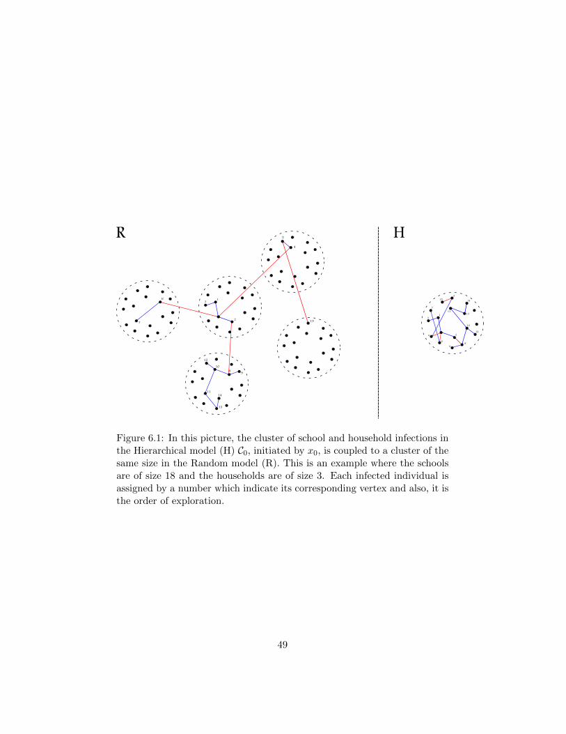
1

2

3

4

6

5

7

89

10

11

12

13

141513

2

8 910

12

11

13

14

6

7

4

5

15

HR

Figure 6.1: In this picture, the cluster of school and household infections inthe Hierarchical model (H) C0, initiated by x0, is coupled to a cluster of thesame size in the Random model (R). This is an example where the schoolsare of size 18 and the households are of size 3. Each infected individual isassigned by a number which indicate its corresponding vertex and also, it isthe order of exploration.

49

tained in C0, all open with probability pG independently of each other. Eachtime a green edge between a vertex in C0 and one of its neighbors is markedas open or closed in the Random model, we give the same mark to the cor-responding green edge in the Hierarchical model. Since we condition on Bn,all endpoints of these green edges are in the beginning of the epidemic, mem-bers of previously uninfected school. Start with considering one endpoint,say xi. We could explore the local epidemic Ci in the Hierarchical model,initiated by xi, and we couple this to a cluster in the Random model in thesame way as described above. We repeat this procedure for all endpointsxj . The newly infected individuals in the obtained clusters Cj could makeglobal connections on their turn, and so on. So we conclude that for allk < n1/2−ε, P[TH(n) ≤ k|Dn] ≥ P[TR(n) ≤ k|Dn].

Corollary 6.3.2. Let qH and qR be the extinction probabilities for corre-sponding branching processes and let E[TH(n)] and E[TR(n)] be the expectedfinal size within a population of size n, for the Hierarchical and the Randommodel respectively. For all transmission rates ( βG

n−1 , βS , βH), we have

qH ≥ qR

andlimn→∞

E[TH(n)] ≤ limn→∞

E[TR(n)].

Proof. By Lemma 5.2.2, we know that in a randomly mixing populationwith infection rate β, there exists a K such that the probability that theepidemic cluster will not be larger than Klog(n) tends to the extinctionprobability of the corresponding branching process, as n goes to infinity.We could apply this lemma directly to the Hierarchical model, since therewe have uniform mixing on school level. For Random model, Lemma 5.2.2have to be generalized to the multi-type uniform mixing case, but the proofis not included in this thesis.For the randomly mixing case, we fix a N and ε > 0, such that for alln > N , Klog(n) < n1/2−ε. So by Lemma 6.3.1, when we choose k ∈(Klog(n), n1/2−ε) and we let n grow to infinity, we get qH ≥ qR. Fur-thermore, we have seen in Theorem 5.2.1 that, given that a large out-break occurs, the proportional final size converges to the corresponding sur-vival probability. So, when we generalize the results of chapter 5 to themulti-type case, the inequality for the extinction probabilities implies thatlimn→∞ E[TH(n)] ≤ limn→∞ E[TR(n)].

The strong relation between both models is also explicitly shown in figure6.2 and 6.3 for a finite population of size 100, where we have calculated

50

the reproduction number and the extinction probability for some modelparameters. In these two examples we have held the relation between thetransmission parameters βH : βS : βG fixed. In figure 6.2 one can see thatfor all (βH , βS , βG) the red line is below the blue line and this is consistentwith Corollary 6.3.2. Remember that Rρ contains different information thanRS , so it is of little use to compare their exact values, hence the intersectionin graphic 6.3 has less meaning. However, Rρ and RS both serve as anepidemic threshold, and they exceed the critical value 1 for the same modelparameters as the extinction probabilities become below 1.

51

0

0.2

0.4

0.6

0.8

1

0 1 2 3 4 5

Exti

nct

ion p

robabili

ty

BetaH

BetaH:BetaS :: BetaG =4:2:1 Hierarchical

Random

Figure 6.2: The extinction probabilities

0

1

2

3

4

5

0 1 2 3 4 5

R

BetaH

BetaH:BetaS :BetaG =4:2:1 Base

HierarchicalRandom

Figure 6.3: The reproduction numbers

52

6.4 Comparison with equal number of neighbors

The strong relation we have proven in Theorem 6.3.1, gives rise to a com-parison of a Hierarchical model and a Random model where the number ofneighbors for each individual are the same in the start of the epidemic. Wecould for instance consider a Hierarchical model with schools of size nS andhouseholds of size 2 and a Random model where the schools are of size nS−1and household of size 2. It is difficult to compare these models exactly, butwe will explain their difference intuitively.Firstly, we remark that although each individual in both models is connectedto (nS − 1) + 1 individuals, in the Hierarchical model one of these neighborshas a higher probability to become infected. This is the sibling, which canbe infected here by school and household contact as well. It seems that thisobservation implies that the Hierarchical model will spread the epidemicmore easily. However, we still have not taken into account that there is alsoa probability that newly infected individuals were already infected before.Especially, in Hierarchical structure this will be more often the case. Re-member that in the Random model, sibling are with high probability mem-ber of previously uninfected schools, while in the Hierarchical model house-hold infection remains within the schools. In the Hierarchical model, infec-tion transmission from school to school is only possible via global contact.By this reasoning, we could expect that for large βH the Random model willspread the disease more quickly while for small βH the Hierarchical modelis more friendly for the epidemic spread. Note that a larger household sizewill only strengthen this effect.These observations are also confirmed in the graphics below, see figure 6.4.We have plotted the reproduction numbers for the Hierarchical and Randommodel for three different values of βH . In particular, look at the differentvalues of βS for which the red ‘Rand3’ lines intersect the base line. Theseintersections indicate the phase transitions in the models.

6.5 Further research

In Theorem 6.3.1 we have proved that in the start of an epidemic, whenthe number of new infected individuals can be approximated by a branchingprocess, the Hierarchical model is in the limit stochastically dominated bythe Random model. However, it is not clear whether this strong comparisonstill holds after the branching approximation breaks down. In this case,the coupling we described above will fail: it is possible that individuals

53

infected via household contact or global contact were already infected beforein the Random model while these ‘same’ individuals were still susceptible inHierarchical model. In order to prove a comparison (if it exists) between theeventually epidemic sizes in both models, a creative way of coupling betweenthe epidemic processes have to be constructed.

54

0.2

0.4

0.6

0.8

1

1.2

1.4

0 1 2 3 4 5

R

BetaS

BetaH =0.1, BetaG=0.3Rand4

Hierar4Rand3

Base

0.2

0.4

0.6

0.8

1

1.2

1.4

1.6

0 1 2 3 4 5

R

BetaS

BetaH =0.21 BetaG=0.3Rand4

Hierar4Rand3Base

0.4

0.6

0.8

1

1.2

1.4

1.6

1.8

R

0 1 2 3 4 5BetaS

BetaH =0.5, BetaG=0.3Rand4

Hierar4Rand3

Base

Figure 6.4: You see the reproduction numbers varying with βS for a Random(resp. Random, Household) model where schools are of size 3 (resp. 4 , 4)and households are of size 2, called ‘Rand3’ (resp. ‘Rand4’, ‘Hierar4 ’). Inthe second plot we have tuned βH = 0.22 such that ‘Rand3’ and ‘Hierar4’has a phase transition for the same βS . Here, βG = 0.3, which is ratherarbitrary. 55

Chapter 7

Discussion

In this chapter we will present some remarks on the assumptions we havemade in the previous chapters.

For ease of presentation we have assumed that the schools (resp. households)in the Random and Hierarchical model are all of the same size. To obtain amodel closer to reality we can easily generalize our results by incorporatingunequal subgroup sizes [3] [4]. We can then do similar computations as inChapter 6, but the set of different types will become much larger. Individu-als in the Random model will then not only be labeled according to whetherthey are infected by household, school or global contact, but the labels willalso have to indicate the size of the subgroup they belong to. In the Hierar-chical model, the spread from school to school should then be approximatedby a multi-type branching process, where the schools are labeled accordingto the number of households of different sizes which it contains.

Another assumption we have made, was that all individuals are infectious fora fixed period of time. Although in reality, the infectious period is differentfor each individual, it is proven [8] [10] that by assuming a fixed infectiousperiod, the actual final epidemic size will be overestimated. So the vacci-nating strategies we have proposed in chapter 6 will at least be sufficient tohalt the spread of an epidemic. This is because when we assume a fixed in-fectious period, our model corresponds to the bond percolation model wherethe infections made by the same individual are independent. Meester andTrapman have presented a proof (based on Kuulasmaa [8]) that the bondpercolation model corresponds to a worst case scenario, in the sense thatthe probability of an individual being part of an infinitely large cluster is

56

maximal, with respect to epidemics with other (random) infectious periods.See Theorem 1.1 of [10] where the susceptibility of all individuals W = 1.

Finally we remark that in [1], [12], [4], and other research, the underlyingsocial network for the spread of an epidemic via global contacts is describedby random graphs (e.g. Erdos Renyi graphs) instead of by a complete graphas we have used. Because in reality it is unlikely that an individual will meetall other individuals during his or her lifetime, the random graph is used toapproximate the actual social network stochastically. In the Erdos Renyigraph, the i-th and the j-th individual are neighbors of each other with acertain probability pc (i.e. they are connected by an edge in the network),and this probability is the same for each pairs of individuals. Secondly, tomodel the spread of global infections across the resulting network, there is anadditional probability pβ (independent of pc) that the infection will actuallytransmit from i to j when i becomes infective earlier than j, or visa versa.However, in the Hierarchical and Random model, we have combined thesetwo processes into one process. Here, the contact probability pG could beviewed as a product of these independent ‘neighbor’ and ‘infection’ (‘closecontact’ in literature) probabilities pc and pβ.

57

Bibliography

[1] Andersson, H. Epidemic models and social networks. MathematicalScientist, 24:128–147, April 1999.

[2] Andersson, H. and Britton, T. Stochastic epidemic models andtheir statistical Analysis. Spring Lecture Notes in Statistics, 2000.

[3] Ball, F.G., Mollison, D., and Scalia-Tomba, G. Epidemics withtwo levels of mixing. Annals of Applied probability, pages 46–89, 1997.

[4] Ball, F.G, Trapman, J.P., and Sirl, D. Threshold Behaviour andfinal outcome of an epidemic on a random network with householdstructure. Advances in Applied probability, 41:765 –796, 2009.

[5] Diekmann, O. and Heesterbeek, J.A.P. Mathematical epidemiologyof Infectious Diseases. Chichester: John Wiley & Son, 2000.

[6] Harris, T.E. The Theory of Branching Processes. Doven Publications,New York, 2nd Edition, 1989.

[7] Hofstad, R. van der. Random graphs and complex networks.http://www.win.tue.nl/ rhofstad/NotesRGCN2009.pdf, 2009.

[8] Kuulasmaa, K. The spatial general epidemic and locally dependentrandom graphs. Advances in Applied probability, 1982.

[9] Meester, R.W.J. and Franscetti, M. Random networks for com-munication, from statistical physics to information systems. CambridgeUniversity Press, 2007.

[10] Meester, R.W.J. and Trapman, J.P. Bounding basic characteristicsof spatial epidemics with a new percolation model. (Submitted), 2008.

[11] Mollison, D. Epidemic models: their structure and relation to data.Journal of applied mathematics, 1977.

58

[12] Trapman, J.P. On stochastic models for the spread of infections. PhDthesis, September 2006.

[13] Watts D.J., Muhamad, R., Medina, D.C., and Dodds, P.S. Mul-tiscale, resurgent epidemic in a hierarchical metapopulation model.PNAS, applied mathematics, 7, 2005.

59