TANF, Childcare and Child

Well-Being in Sole-Parent Families

Marianne Bruins∗

24 August 2017

Abstract

I estimate a structural model of sole-parent families to analyse the impact of TANF.

Its benefits fail to reach the poorest mothers, who typically prefer not to meet the 30

hr/wk work requirement. Using the model to measure the intra-household allocation

of resources, I find that poverty rates among children of sole mothers have risen by

four percentage points since 1996. I compare TANF to alternative policies, such as

free childcare, which promote labour supply by increasing the returns to work. Such

policies are more than twice as effective at targeting household resources to children,

per dollar spent.

∗Email: marianne.bruins@economics.ox.ac.uk. Nuffield College and Department of Economics, Uni-versity of Oxford. This research has greatly benefited from discussions with R. Blundell, S. Bond, M. Brewer,M. Browning, J. Duffy, J. Fenske, C. Meghir, S. Quinn, J. Ziliak and comments from seminar participantsat Oxford and ISER (Essex). The author thanks the British Academy for funding (Award no. SG152880).This work was supported by the HPC facilities operated by, and the staff of, the Yale Center for ResearchComputing.

i

Contents

1 Introduction 1

2 Background 42.1 Welfare programmes and reform . . . . . . . . . . . . . . . . . . . . . . . . . 42.2 Trends in household behaviour since 1996 . . . . . . . . . . . . . . . . . . . . 7

3 Structural model 93.1 Preferences . . . . . . . . . . . . . . . . . . . . . . . . . . . . . . . . . . . . 103.2 Constraints . . . . . . . . . . . . . . . . . . . . . . . . . . . . . . . . . . . . 133.3 Solution and two-stage budgeting . . . . . . . . . . . . . . . . . . . . . . . . 13

4 Estimation procedure 154.1 Data sources . . . . . . . . . . . . . . . . . . . . . . . . . . . . . . . . . . . . 164.2 Simulated method of moments . . . . . . . . . . . . . . . . . . . . . . . . . . 194.3 Imputation (via simulation) of missing variables . . . . . . . . . . . . . . . . 214.4 Sample moments: selection and construction . . . . . . . . . . . . . . . . . . 234.5 Identification of structural parameters . . . . . . . . . . . . . . . . . . . . . 264.6 Identifying the TANF enrolment disutilities . . . . . . . . . . . . . . . . . . 27

5 Estimates and model fit 285.1 Parameter estimates . . . . . . . . . . . . . . . . . . . . . . . . . . . . . . . 295.2 Model fit: in-sample performance . . . . . . . . . . . . . . . . . . . . . . . . 315.3 Model fit: external validation . . . . . . . . . . . . . . . . . . . . . . . . . . 355.4 Identification: a numerical analysis . . . . . . . . . . . . . . . . . . . . . . . 36

6 Child welfare, TANF and alternative policies 386.1 Child welfare in the welfare-to-work era . . . . . . . . . . . . . . . . . . . . . 406.2 PROWRA, child welfare and maternal labour supply . . . . . . . . . . . . . 436.3 Alternatives to welfare-to-work programmes . . . . . . . . . . . . . . . . . . 466.4 Implications for welfare policies . . . . . . . . . . . . . . . . . . . . . . . . . 50

7 Conclusion 51

8 References 52

Appendices (for online publication)

A Data sources and construction A1

B Estimation procedure: further details A3

C Parameter estimates A7

D Calculation of taxes and welfare payments A12

ii

E Policy counterfactuals: full listing of results A15

iii

1 Introduction

The introduction of welfare-to-work programmes, in many OECD countries, has been the

most significant change to cash welfare in the postwar era. These programmes are designed to

reduce welfare dependency by tying eligibility to work requirements. They were introduced

with a limited understanding of their direct impact on child welfare, in spite of the welfare and

economic opportunities of disadvantaged children being the focus of other policy initiatives.

In this paper I open the black box of household behaviour to examine how welfare-to-

work programmes influence the allocation of household resources to children. That this

remains poorly understood is perhaps not surprising, given the taxing data requirements and

sophisticated modelling of households’ preferences and the tax and welfare system necessary

to answer this question. But it is of pressing concern in view of the extensive evidence

suggesting that what goes on within the household is crucial for children’s immediate welfare

and outcomes later in life.

In the US, the major policy reform of this kind was effected with the introduction of

Temporary Assistance for Needy Families (TANF) in 1996, which replace the existing cash

welfare programme designed for sole mothers. This paper provides a detailed analysis of

how TANF affected the allocation of household resources to children over 1996–2008, and to

the best of my knowledge is the first paper to do so. My analysis is based on a structural

model of household decision-making – estimated on a sample of sole mothers (without a

college degree) – in which children benefit from consumption, time with their mother, and

a domestically produced public good. With the estimated model, I am able to perform a

comprehensive analysis of the impact of the introduction of TANF on child welfare. I also

consider how welfare policies might be designed so as to better target household resources to

children, while still meeting TANF’s original objective of promoting female labour supply.

Using the estimated model, I demonstrate that, at 30 hours per week (hr/wk), the work

requirements for TANF are set so high that many low-wage mothers would be better off

spending their time in activities other than market work, than meeting the work requirements

and receiving TANF payments -- even though their weekly earnings put them well below

the poverty line. For this group, the main consequence of welfare-to-work reforms has been

simply a withdrawal of the benefits to which they had previously been entitled. This loss

of income has been mostly offset by an increase in their labour supply of around 5 hr/wk,

primarily at the expense of time spent in housework.

Accordingly, poverty measures based on household-level income and consumption have

indicated no increase in child poverty rates since 1996 (Blank, 2002; Meyer and Sullivan,

2004). But such measures fail to account for the decline in mothers’ time available for

1

activities outside market work, and the subsequent decline in home production which has

negatively affected children. I therefore use the model to construct a measure of child

poverty which is based on the resources children actually receive from the household, and

thus appropriately values the time mothers spend with their children, and fully accounts for

home production. I find that, once the intra-household allocation of resources is accounted

for in this manner, child poverty has in fact increased by four percentage points since the

introduction of TANF.

I also use the model to perform a number of counterfactual experiments, so as to evaluate

the consequences of both actual and hypothetical welfare reforms. As discussed above,

few sole mothers enrol in TANF and meet the work requirements, so TANF only provides

meaningful work incentives for a very small group of mothers, less than five per cent of my

sample. In contrast, the Earned Income Tax Credit (EITC), an in-work subsidy, raises the

net returns to work for all households with sufficiently low incomes. Thus, it is not surprising

that I find the EITC to be more effective than TANF at promoting maternal labour supply.

I also find the EITC to be twice as efficient at targeting resources to children, measured

in terms of the (money-metric) improvement in children’s welfare per (net) dollar spent on

the policy. (This calculation of ‘net spending’ on the EITC – and on other programmes

– fully accounts for its secondary effects on government tax revenues, due to households’

behavioural responses.)

These results motivate me to consider a number of alternative policies that similarly

promote labour supply by increasing the returns from working. These alternative policies

take the form of childcare subsidies and wage subsidies. Their main point of difference from

the EITC lies in that they pay benefits that are proportional to hours worked, rather than

to total earnings. One drawback of a policy whose benefits are contingent on total earnings,

instead of hours worked, is that it fails to distinguish between e.g. two mothers, one of who

works part time and the other full time, but who have the same total earnings. Clearly, in

such a case, the mother working part time will be able to devote more time to housework

and children, both of which contribute to children’s welfare, and thus her children may be

considerably better off than those of the mother working full time.

My analysis of these alternative policies reveals that they are indeed more effective than

TANF and the EITC at increasing maternal labour supply, and twice as efficient as TANF

at targeting household resources to children. More specifically, among the policies I consider

are the provision of free childcare, and two wage subsidies: a flat-rate wage subsidy of $1/hr,

and a targeted wage subsidy which brings all wages up to $11.60/hr (both in 2000 dollars).1

1This is equivalent to $15/hr in 2016 dollars, which compares to the $15/hr minimum wage scheduledfor New York in 2018.

2

For both the free childcare and targeted wage subsidies, the extent to which expenditure

on these policies passes through to children is comparable to the EITC, at $0.41 and $0.50

of every (net) dollar spent, respectively. The $1/hr wage subsidy has a pass-through rate

almost twice that of the EITC, at $0.76 per dollar spent. To the best of my knowledge,

the favourable effects of such policies on children have not previously been identified, most

likely because their impact on the allocation of resources within the household has not been

properly understood accounted for.

In recent decades, many OECD countries have increased childcare subsidies, and in a

few cases have provided universal free childcare. Recent literature examining the effects of

these policies on the cognitive and non-cognitive development of young children has focused

largely on the relative quality of care available at home and at centres. My analysis identifies

a secondary channel through which such policies may improve child welfare: by making

additional household resources available to children. In quantitative terms, I find that for

each (net) dollar spent on such policies, $0.50 gets through to children. Depending on the

household’s income level, either channel – the relative quality of care, or the allocation

of household resources to children – may predominate: and my results suggest that the

household allocation channel is particularly relevant for children in low-income households.

To account for the benefits children derive from maternal time spent in activities aside

from paid work, the structural model developed here contains a detailed treatment of moth-

ers’ time use. This is facilitated by the use of time diary data, which allows me to construct a

measure of parents’ time with children that aggregates those activities that the literature has

identified as being important for child development. To keep the complexity of the modelling

and the estimation procedure within reasonable bounds, while allowing for such a detailed

treatment of the household’s allocation and budget constraint, I abstract as far as possible

from the intertemporal aspects of the household’s decision making. The structural model

is therefore static – but I am careful to ensure that the solution to the model is consistent

with that of the household’s intertemporal choice problem. This consistency permits the

parameters of the structural model to be identified from data on households’ actual choices,

even though those choices arise from intertemporally optimising behaviour.

Methodologically, this paper demonstrates how to combine separate time-use and con-

sumption datasets to estimate a model of household resource allocation, yielding much larger

sample sizes and more precise estimates.2 (Estimation by simulated method of moments is

necessary here due to the use of these multiple datasets.) Only a few datasets provide both

2The datasets drawn used are: American Time Use Survey (ATUS, 2003–08), the American HeritageTime Use Survey (AHTUS, 1995), the Consumer Expenditure Survey (CE, 1993–2008), the Current Pop-ulation Survey (CPS, 1993–2008) and the Survey of Income and Program Participation (SIPP, 1996, 2001,2004, and 2008).

3

types of data, and those that do have only a small number of observations, which is partic-

ularly problematic in this context due to the measurement error problems associated with

time diaries and consumption data. On the other hand, estimating the model with only con-

sumption data – as has been the practice in much of the previous empirical work involving

these models – means that the additional information on the household allocation provided

by time-use data is ignored. By examining how the (estimated) asymptotic variances of the

parameter estimates would be altered if certain groups of moments were ignored, I obtain

empirical evidence that the use of moments derived from time-use data significantly improves

the precision of the estimates.

Outline The remainder of this paper is organised as follows. Section 2 provides more de-

tailed background information on changes in welfare policy over the sample period (1993–2008),

and observed trends in the behaviour of sole-mother households over this period. The struc-

tural model, and the procedure used to estimate it, are elaborated in Sections 3 and 4.

Section 5 presents parameter estimates and analyses the model’s fit. Section 6 presents the

main findings of the paper: here I develop money-metric measures of child welfare, provide

estimates of the effect of TANF on child poverty rates, and use the model to perform a

series of counterfactual experiments, to evaluate a range of alternatives to TANF. Section 7

concludes.

2 Background

In this section I discuss the introduction of TANF, and other welfare programme reforms

that occurred over 1993–2008. I then describe some of the trends in sole mothers’ behaviour

during this period: the most striking of which is a reallocation of around 5hr/wk from

market work to home production. These trends suggest that standard measures of child

welfare, such as the official poverty measure, that fail to account for the value of mothers’

time spent in activities aside from market work, would give a misleading impression of the

impact of TANF on child welfare. (I later return to this issue in Section 6, where I use the

model to evaluate the totality of resources allocated to children, including time with parents

and the provision of a public good, and consider how this has changed since 1996.)

2.1 Welfare programmes and reform

TANF and AFDC The Personal Responsibility and Work Opportunity Reconciliation

Act of 1996 (PRWORA) effected the greatest change in the US welfare system since the

4

New Deal, by replacing Aid to Families with Dependent Children (AFDC) – the main cash

welfare programme available to sole mothers – with Temporary Assistance for Needy Families

(TANF). Unlike AFDC, TANF imposes: (a) lifetime limits on receipt, allowing individuals to

claim benefits for a maximum of five years; and (b) work requirements, which make eligibility

contingent on working a certain number of hours (usually 30) per week. (Although AFDC

did impose some work requirements, these were much more limited in extent.) In practice,

these work requirements have been unevenly enforced, with certain activities permitted to

substitute for paid employment, such as actively searching for work or participation in a job

training programme. Indeed only a third of TANF recipients worked in 2008, the final year

of the sample period.

PRWORA granted states greater discretion over the provision of TANF than they had

been allowed over AFDC: in the setting of eligibility rules, benefit levels, and the extent to

which non-compliance with work requirements are penalised. The result is considerable het-

erogeneity in the way TANF is administered across states, as illustrated for example by the

marked differences in the generosity of benefits provided in California and Texas, displayed

in panels (a) and (b) of Figure 1. Some states, such as Alabama, in addition to the five-

year lifetime limit, prohibit individuals from receiving TANF for more than two consecutive

years, whereas others, such as Michigan, draw upon their own funds to extend payments to

individuals who have exceeded the five-year limit. States have also exercised their autonomy

to redirect federal funding for TANF away from cash welfare, towards such services as mar-

riage counselling, family planning, training programmes, and childcare subsidies. Thus in

aggregate, only 28 per cent of the federal block grant is spent on by cash welfare payments; a

further 16 per cent is spent on childcare subsidies, and 17 per cent on administration (Schott,

Pavetti, and Finch, 2012).

Other programmes While this paper is principally concerned with the impact of TANF

on sole-parent households, the estimation of my structural model requires a comprehensive

modelling of the entire tax and welfare system. In addition to AFDC and TANF, the

model used in this paper accounts for all state and federal taxes on earned incomes, and

the most significant transfer expenditures and welfare programmes targeted at children,

excluding those related to healthcare. The four largest are the Child Tax Credit (CTC), the

Supplemental Nutrition Assistance Program (SNAP), the Dependent Exemption, and the

Earned Income Tax Credit (EITC) (see Isaacs, Toran, Hahn, Fortuny, and Steuerle, 2012);

to these I add the Child and Dependent Care Tax Credit (CDCTC). Any state-level variation

in these programmes (where applicable) is accounted for in the model; see Appendix D for

further details.

5

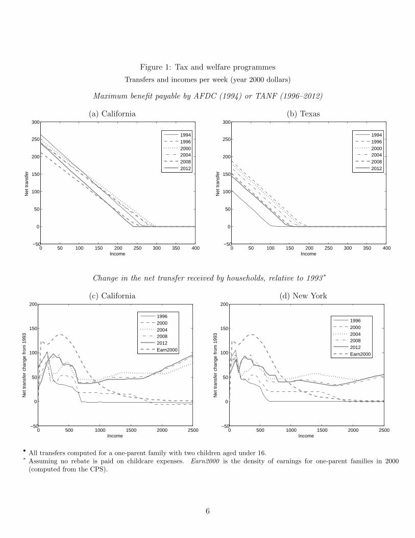
Figure 1: Tax and welfare programmes

Transfers and incomes per week (year 2000 dollars)

Maximum benefit payable by AFDC (1994) or TANF (1996–2012)

(a) California (b) Texas

0 50 100 150 200 250 300 350 400−50

0

50

100

150

200

250

300

Income

Net

tran

sfer

199419962000200420082012

0 50 100 150 200 250 300 350 400−50

0

50

100

150

200

250

300

Income

Net

tran

sfer

199419962000200420082012

Change in the net transfer received by households, relative to 1993 ∗

(c) California (d) New York

0 500 1000 1500 2000 2500−50

0

50

100

150

200

Income

Net

tran

sfer

cha

nge

from

199

3

19962000200420082012Earn2000

0 500 1000 1500 2000 2500−50

0

50

100

150

200

Income

Net

tran

sfer

cha

nge

from

199

3

19962000200420082012Earn2000

• All transfers computed for a one-parent family with two children aged under 16.∗ Assuming no rebate is paid on childcare expenses. Earn2000 is the density of earnings for one-parent families in 2000

(computed from the CPS).

6

Panels (c) and (d) of Figure 1 plot the change in the net transfer received, under the

foregoing taxes and welfare programmes, by a one-parent household with two children in

California and New York, relative to 1993 (adjusted for inflation). These illustrate that,

aside from the introduction of TANF in 1996, there have been substantial changes to the tax

and welfare system at both the state and federal level over the sample period (1993–2008),

something which aids the identification of the structural model’s parameters.

2.2 Trends in household behaviour since 1996

One of the major objectives of TANF was to reduce welfare dependency, and since 1996 there

has been a marked decline in caseloads: by 2008, the number of TANF enrollees had fallen

by two-thirds (see panel (a) of Figure 2). The other major aim of TANF was to promote

employment: panel (b) shows that hours worked by single mothers (without a college degree)

indeed increased over the same epoch.

This paper focuses on the impact of TANF on the allocation of resources within the

household, particularly on the resources allocated to children. Panels (d)–(f) display trends

in household income and food expenditures separately for single women with children (S1)

and without (S2), controlling for the number of children, age, education, race, and state (see

the notes to the figure for further details). This extends Meyer and Sullivan’s (2004) analysis

out to 2010: and as in their work, the comparison allows me to control for any shocks that

would have affected both groups similarly, such as a change in the relative price of food

away from home. Any remaining differences in these trends may therefore be ascribed to

something that has affected single women with children differently from those without, the

introduction of TANF being a plausible candidate.

Meyer and Sullivan (2008) find that sole mothers have increased their hours worked since

1996, and that this has come at the expense of non-market work. Consistent with Meyer

and Sullivan (2008), I find a decline in housework of around 5 hr/wk between 1993 and

2008 (see panel (c)). I also find that sole mothers have increased their expenditure on food

away from home, a trend not observed for single women without children (panel (e)). In

contrast, expenditure on food at home for sole mothers has declined, if anything (panel

(f)). Before-tax income also increased significantly for single women with children, but not

for those without, reflecting the increase in their labour supply (panel (d)). Overall, these

figures illustrate a decline in home production and an increase in market work following the

introduction of TANF.

Standard measures used to evaluate how children welfare has changed since the introduc-

tion of TANF are based on income or consumption at the household level, and do not take

7

Figure 2: Trends in sole mothers’ behaviour

(a) Participation in TANF (proportion) (d) Before-tax income ($/wk)∗

1993-95 1996-99 2000-04 2005-08 2009-12

0.05

0.1

0.15

0.2

0.25

0.3

0.35

0.4

0.45

0.5

estimate

1991-95 1996-99 2000-03 2004-07 2008-10

Parent income percentile

-1.5

-1

-0.5

0

0.5

1

1.5104

estimate (S1)CI upper (S1)CI lower (S1)estimate (S2)CI upper (S2)CI lower (S2)

(b) Housework (hr/wk) (e) Food away from home ($/wk)∗

1993−95 1996−99 2000−04 2005−08 2009−1210

11

12

13

14

15

16

17

18

19

20

1991-95 1996-99 2000-03 2004-07 2008-10

Parent income percentile

-1500

-1000

-500

0

500

estimate (S1)CI upper (S1)CI lower (S1)estimate (S2)CI upper (S2)CI lower (S2)

(c) Hours worked (hr/wk) (f) Food at home ($/wk)∗

1993−95 1996−99 2000−04 2005−08 2009−1220

22

24

26

28

30

32

34

36

1991-95 1996-99 2000-03 2004-07 2008-10

Parent income percentile

-1500

-1000

-500

0

500

estimate (S1)CI upper (S1)CI lower (S1)estimate (S2)CI upper (S2)CI lower (S2)

• Sole mothers without a college degree. Sources: CPS (panels (a)–(b)); A(H)TUS (panel (c)); CE (panels (d)–(f)). Dollarvalues are in year 2000 dollars.

∗ Panels (d)–(f) extends the work of Meyer and Sullivan (2004) to 2010. Figures report coefficients on time dummies (1993–95,1996–99, 2000–03, 2004–07 and 2008–10), interacted with whether or not the single woman has a child (S1: has a child; S2:does not); base case is a single woman with children in 1993–95. Coefficients are estimated by an OLS regression of thereported outcome on the the preceding dummies, and additionally controls for: the number of children, the woman’s age,education (high school, some college dummies), race (black, white dummies), and region (nine) fixed effects.

8

into account home production, the value of maternal time in activities other than market

work, and the distribution of resources within the household. The structural model estim-

ated in this paper will subsequently be shown to closely match the trends described above

(see Section 5.2), and will also allow me to uncover the underlying changes in child welfare

(see Section 6.2).

3 Structural model

The model elaborated in Section 3.1–3.2 (henceforth ‘the structural model’) provides a de-

tailed treatment of maternal time use: both to explain the trends described above, and

because the allocation of maternal time not spent in market work – i.e. between leisure,

time with children and housework – is likely to be important for child welfare. It differs

from other household models estimated in the literature along two dimensions (see e.g. Apps

and Rees, 1996; Cherchye, De Rock, and Vermeulen, 2012; Blundell and Shephard, 2011).

Firstly, child utility is modelled separately from mothers’ utility and the home production

of a public good. Secondly, children’s utility depends on this public good, which is produced

from mother’s time in housework and public consumption expenditures. As I only observe

data on the inputs into the children’s utility function, its shape is determined by the mother’s

choices regarding the allocation of household resources. (Thus a key assumption underlying

the welfare analysis of Section 6 below is that the mother is altruistic towards her children.)

To keep the complexity of the modelling and the estimation procedure within reasonable

bounds, I abstract as far as possible from the intertemporal aspects of the household’s

decision making. The structural model developed below is therefore static: it describes the

household’s resource allocation problem within a given period. I discuss in Section 3.3 how

the solution to the structural model may be rendered consistent with that of the household’s

intertemporal choice problem. This consistency permits the parameters of the structural

model to be identified from data on households’ actual choices, even though those choices

arise from the households’ intertemporal optimisations. My arguments here build upon the

two-stage budgeting approach of Blundell and Walker (1986), extended so as to take account

of the intertemporal aspects of TANF enrolment (due to lifetime limits). I also discuss how

the estimated model may be used to reliably evaluate counterfactual changes to the tax and

welfare system, subject to the qualifications discussed at the end of Section 3.3.

9

3.1 Preferences

The mother’s utility is a weighted sum of: her private utility, u; the children’s utility, K; a

disutility τ from participating in the labour force; and a disutility, ψ, from being enrolled in

AFDC/TANF,

U = u+ δkK − τ · 1hm > 0 − ψ · d, (3.1)

where hm denotes (weekly) hours in paid employment, and d = 1 if the mother enrols in

TANF (and is zero otherwise). Her private utility has the CES form

u(cm, lm, q) = log(γ1−ηmm,c cηmm + γ1−ηm

m,l lηmm + γ1−ηmq,l qηm)1/ηm (3.2)

where cm denotes mother’s consumption, lm leisure, and q the public good. (γm,c + γm,l +

γm,q = 1; and γm,c, γm,l, γm,q ∈ [0, 1], ηm ≤ 1.)

As noted above, I model children’s utility separately from their mother’s, to facilitate

the measurement of child welfare. Children’s utility takes as inputs: mother’s time with

children tm; children’s private consumption, ck; and the (home-produced) public good, q; it

is assumed to have the CES form

K(ck, tm, q) = log(γ1−ηkk,c cηkk + γ1−ηk

k,t tηkm + γ1−ηkk,q qηk)1/ηk (3.3)

(γk,c+γk,t+γk,q = 1; and γk,c, γk,t, γk,q ∈ [0, 1], ηk ≤ 1). I include mothers’ time with children

in the model, because it has been demonstrated to be important for children’s cognitive and

non-cognitive development (see e.g. Brooks-Gunn and Markman 2005; ?; Phillips 2011). The

constant elasticity of substitution (CES) functional form adopted here nests (at ηk = 0) the

Cobb-Douglas specification that has been used in some previous work (see e.g. Del Boca,

Flinn, and Wiswall, 2014).

The quantity of the public good produced by the household is given by the (constant-

returns-to-scale) CES production function

q(cq, qm) = (γ1−ηqq,c c

ηqq + γ

1−ηqq,m q

ηqm )1/ηq ,

where qm denotes the mother’s time devoted to housework, and cq the expenditure on con-

sumption goods which are used as inputs in the production of the public good, which I refer

to as ‘public consumption’. (γq,c + γq,m = 1; and γq,c, γq,m ∈ [0, 1], ηq ≤ 1.) This CES

specification has been used in prior literature to model home production (see e.g. Aguiar

and Hurst, 2007).

10

AFDC/TANF enrolment The AFDC/TANF enrolment disutility ψ decomposes as

ψ = ψst + ψit. (3.4)

ψst represents the ‘static’ non-pecuniary costs incurred when enrolling in AFDC/TANF.

For example, to be eligible for TANF payments without meeting the work requirements,

a mother would usually need to be engaged in certain other activities, such as actively

searching for work or participating in a job training programme. (The extent of federal

funding that states receive for TANF is related to the proportion of their caseload meeting

the work requirements, and thus states generally make it more difficult for individuals to

participate in TANF without meeting these requirements.) Those who do meet the work

requirement still face non-negligible administrative costs of applying for benefits. ψst is

accordingly allowed to vary, depending on whether or not work requirements are met (or in

the case of AFDC, whether or not the mother works).

ψit is intended to capture the ‘intertemporal’ cost of enrolling in TANF in the current

period, due to foregoing the option of enrolling in (a year’s worth of) TANF in the future.

(ψit is therefore set to zero for AFDC.) As discussed in Section 3.3 below, ψit is needed to

make the structural model consistent with the mother’s intertemporal optimisation problem.

(See Section 4.6 below for the moments used to separately identify ψst and ψit.)

Receipt of other transfers and benefits Participation in the other transfer programmes

considered in this paper – the EITC, SNAP, CTC and the CDCTC – is not modelled. Rather,

when calculating the household’s after-tax income (see Section 3.2 below) it is assumed that

eligible households always receive the payments (or tax credits) to which they are entitled.

Relative to TANF, which had a take-up rate of around 30.7 per cent in 2013 (Crouse and

Macartney, 2016), the take-up rates for these programmes are much higher, so this seems an

acceptable simplifying assumption. (According to Dahl and Lochner (2011), the take-up rate

for the EITC was over 80 per cent in every year of the sample period, while that for SNAP

always exceeded 50 per cent, reaching a maximum of 87 per cent in 2007). Moreover, TANF’s

job search and training requirements impose burdens on enrollees that have no counterpart

in these other programmes.

Preference heterogeneity and parametrisation To permit heterogeneity in prefer-

ences, a number of parameters are allowed to vary with both observables and unobservables.

In the following paragraphs, ε signifies an i.i.d. standard normal disturbance (all of which

are mutually uncorrelated), and x a vector of observed household characteristics.

11

Regarding the mother’s preferences, her weight on the child’s utility is parametrised as

δk = exp(x′δβδ + σδεδ), (3.5)

where xδ includes a constant, and dummies for: the presence of two or more children, and

a child aged five or under. To ensure that the mother’s utility weights γm,· satisfy the the

stipulated adding-up and range constraints, I first specify

γm,c = exp(x′m,cβm,c + σm,cεm,c) γm,l = exp(x′m,lβm,l + σm,lεm,l) γm,q = 1

where xm,l and xm,q both include a constant and an education dummy (indicating whether

the mother has some tertiary education), and xm,l additionally includes the residual from

the mother’s wage equation (see Section 4.3 below). The utility weights are then constructed

from the γm,· as per γm,i = γm,i/∑

j∈c,l,q γm,i for i ∈ c, l, q. The parameter governing the

elasticity of substitution is specified as

ηm = 1− exp(x′m,ηβm,η)

where xm,η = xδ above.

The children’s utility weights are specified as γk,i = γk,i/∑

j∈c,t,q γk,i, where

γk,c = exp(x′k,cβk,c + σk,cεk,c) γk,t = exp(x′k,tβk,t + σk,tεk,t) γk,q = 1

and xk,c and xk,t both include a constant and a dummy for the presence of a child aged five

or under. The elasticity is parametrised as ηk = 1 − exp(x′k,ηβk,η), where xk,η additionally

includes a dummy for the presence of two or more children. The public good production

weights γq,· are constructed analogously from

γq,c = exp(x′q,cβq,c + σq,cεq,c) γq,m = 1,

while ηq = 1 − exp(x′q,ηβq,η), where both xq,c and xq,η include a constant and a dummy for

the presence of a child aged five or under.

The enrolment disutilities ψst and ψit are parametrised as exp(x′β + σε), where ε is a

standard Gaussian disturbance. For ψst, x consists of dummies for the year groups 1993–95,

1996–99, 2000–04, and 2005–08; both β and σ are allowed to vary depending on whether the

mother meets the mandated work requirements (for TANF; for AFDC, it varies according to

whether or not she works). For ψit, x collects the same year group dummies, and additionally

dummies for the presence of: two or more children, and a child aged five or under.

12

3.2 Constraints

The mother’s utility in (3.1) will be maximised subject to her time and budget constraints.

I also discretise hours choices so that sole mothers choose their hours of work hm from

H = 0, 10, 20, 30, 40, 50, 60. This may be justified by the presence of frictions in the labour

market (see Hoynes, 1996; Blundell and Shephard, 2011) and simplifies the computation

of the household’s optimal choices, which would otherwise be greatly complicated by the

non-convexity of the budget set.

The mother’s (weekly) time constraint is

lm + hm + tm + qm ≤ 105, (3.6)

(nine hours per day are excluded for sleep and personal care). The budget constraint is

cm + ck + cq︸ ︷︷ ︸non-durablesconsumption

+ no5po5[hm − ao5 − 30]+︸ ︷︷ ︸cost of childcare

for children aged 6–13

+ nu5pu5[hm − au5]+︸ ︷︷ ︸cost of childcare

for children aged 0–5

≤ e(hm, wm; d) + y − s (3.7)

where: [x]+ = maxx, 0; and for children aged 6–13, po5, ao5, and no5 respectively denote the

price of childcare, the hours of informal free childcare available (such as would be provided by

a neighbour or relative), and number of children (and pu5, au5 and nu5 similarly for children

aged 5 and under). Note that the ‘30’ in equation (3.7) reflects the 30 hr/wk that children

aged 6–13 would spend in school. y denotes nonlabour income, s savings, wm the mother’s

wage, hm her hours worked, and e(hm, wm; d) her implied after-tax earnings. Recall that

d = 1 if the mother elects to receive TANF payments; and zero otherwise.

Calculation of after-tax income e(·) includes: taxes at the federal and state levels; tax

credits (EITC, CTC, CDCTC); SNAP (‘food stamps’); and AFDC/TANF (see Section 2.1

above and Appendix D for further details). As noted above, for all programmes except TANF

it is assumed that the household always receives the full transfer for which it is eligible. I

also assume that SNAP receipts are always less than the household’s desired expenditure on

food, and so can be treated as a pure cash transfer.

3.3 Solution and two-stage budgeting

Solving the static model Let C = (cm, ck, cq, lm, hm, tm, qm) denote the mother’s choices

over time and expenditure, and

U(C) = u[cm, lm, q(qm, cq)] + δkK[ck, tm, q(qm, cq)] (3.8)

13

her total utility, abstracting from TANF enrolment costs. Given y − s and her TANF

enrolment status d ∈ 0, 1, her feasible set of choices C(y − s, d) is determined by her

weekly time and budget constraints ((3.6) and (3.7)); recall that I also require hm ∈ H.

Thus according to the model above (‘the structural model’) her optimal choices for C and d

may be determined by solving

maxd∈0,1

maxC∈C(y−s,d)

U(C)− d · ψ = maxd∈0,1

max

C∈C(y−s,d)U(C)− d(ψst + ψit)

. (3.9)

I now turn the question of how the structural model may be reconciled with the mother’s

intertemporal decision problem.

Two-stage budgeting A sole mother may be regarded as solving an intertemporal de-

cision problem, the solution to which involves choices over: (i) savings (or equivalently,

asset holdings), (ii) enrolment in TANF, and (iii) the allocation of time and income within

each period. My structural model is concerned with the second and third of these choices.

The modelling of TANF enrolment is complicated by the presence of lifetime limits, which

give TANF enrolment an intertemporal aspect that is not shared by other welfare pro-

grammes. Together with the mother’s (unmodelled) savings decision, this raises two issues.

The first concerns whether the parameters of the structural model can be identified from

data on household’s choices, given that those observed choices arise from the solution to

those household’s intertemporal optimisation problems. This will be the case if the solutions

to the structural model and intertemporal choice problem are consistent with each other;

such consistency is established immediately below. The second issue, which is discussed

at the end of this section, concerns the extent to which the model can be reliably used to

conduct counterfactual experiments.

In view of (3.8) above, and recalling that ψst embodies the ‘static’ cost of enrolling in

TANF (see Section 3.1 above), assuming additive separability the mother’s intertemporal

problem may be put into recursive form as

V(A,D) = maxs∈R

maxd∈0,1

max

C∈C(y−s,d)U(C)− d · ψst + ρEV [A′(s), D + d]

, (3.10)

where A denotes her asset holdings, D ≤ 5 the number of times that she has enrolled in

TANF prior to the current period, V is the current value of the problem, ρ is the mother’s

discount rate, and E is computed conditional on the information available in the current

period. Asset holdings A′ in the next period evolve according to A′(s) = (1 + r′)(A + s),

where r′ is the (unknown) rate of return on the household’s portfolio between the current

14

period and the next; non-labour income in the next period is given by y′ = r′(A+ s).

A key implication of (3.10) is the following. Conditional on her (optimal) choices of

s and d, the mother’s optimal choice of C may be computed simply by maximising U(C)over C(y − s, d). This corresponds exactly to the maximisation problem (3.9) solved in the

structural model, with respect to the C variables. So far as TANF enrolment (d) is concerned,

it is also evident from (3.10) that the mother chooses to enrol (d = 1) if and only if

maxC∈C(y−s,1)

U(C)− maxC∈C(y−s,0)

U(C) ≥ ψst + ρEV [A′(s), D]− V [A′(s), D + 1]

= ψst + ψit.

I interpret the second term on the r.h.s. of the inequality as the ‘intertemporal cost’ of

enrolling in TANF, due to foregoing the option of (a year’s worth of) TANF in the future;

this term is subsumed in ψit in the structural model. Although ψit should depend on the

household’s current levels of A and D, I do not observe these variables, and thus any variation

in these across the sample is treated as a form of unobservable heterogeneity, i.e. it is absorbed

into the stochastic component of ψit. (Regarding the separate identification of ψst and ψit,

see Section 4.6 below.) Thus by including ψit in the structural model, the solution to that

model (for C and d) can be made consistent with that of the household’s intertemporal

optimisation, thereby permitting the identification (and thence estimation) of the structural

model’s parameters.

Regarding the counterfactual exercises conducted in Section 6 below, in most of these

TANF is eliminated and replaced by an alternative policy – the parameters of TANF itself

are not adjusted. In such cases, the question of how the (unmodelled) intertemporal trade-

offs related to TANF enrolment might be altered by the counterfactual policy simply does

not arise. On the other hand, I must assume that savings decisions – also omitted from

the structural model – are not materially different under the counterfactual. I justify this

on the grounds that sole mothers – particularly those with lower earnings, and who are

therefore more likely to be eligible for cash welfare – have low asset holdings (Del Boca,

Flinn, and Wiswall, 2014) and behave essentially as hand-to-mouth consumers. Moreover,

the hypothetical policy changes that I consider are intended to be permanent: and as such

would induce less substitution in consumption across time periods than a temporary policy

change.

4 Estimation procedure

I estimate the structural model using simulated method of moments (SMM), drawing upon

multiple datasets to build up an accurate picture of the allocation of household resources. To

15

estimate the model using only one dataset would require that dataset to contain both time

use and consumption data. Such datasets are particularly rare: the most notable instances

of previous work estimating household models using only one dataset have involved either

the Panel Study of Income Dynamics (Child Development Supplement) or the Longitudinal

Internet Studies for the Social Sciences (a Dutch panel), as used by Del Boca, Flinn, and

Wiswall (2014) and Cherchye, De Rock, and Vermeulen (2012) respectively. The small size

of these datasets, particularly for the subgroup of sole mothers considered here (considerably

less than 500 observations in either survey) is problematic due to the measurement errors

associated with time diaries and expenditure surveys.

Moreover, because I will subsequently consider counterfactual policy interventions that

differentially affect households according to their income level, the model needs to accur-

ately describe the full distribution of household behaviours. Accordingly, as discussed in

Section 3.1 above, the model’s parametrisation allows for much behavioural heterogeneity

across households. The estimation of such a richly parametrised model by SMM requires

a collection of sample moments that is highly informative as to the distribution of the al-

location of household resources. This makes accurate data on the full range of household

choices highly valuable, and for this reason I draw upon five datasets to estimate the model,

as explained in Section 4.1.

The mechanics the of the estimation procedure are described in Sections 4.2–4.3. The

choice of sample moments, and the identification of the model parameters, are discussed

in Sections 4.4–4.5, following which I address the problem of how the static and intertem-

poral costs of TANF enrolment (ψst and ψit) may be separately identified and estimated

(Section 4.6).

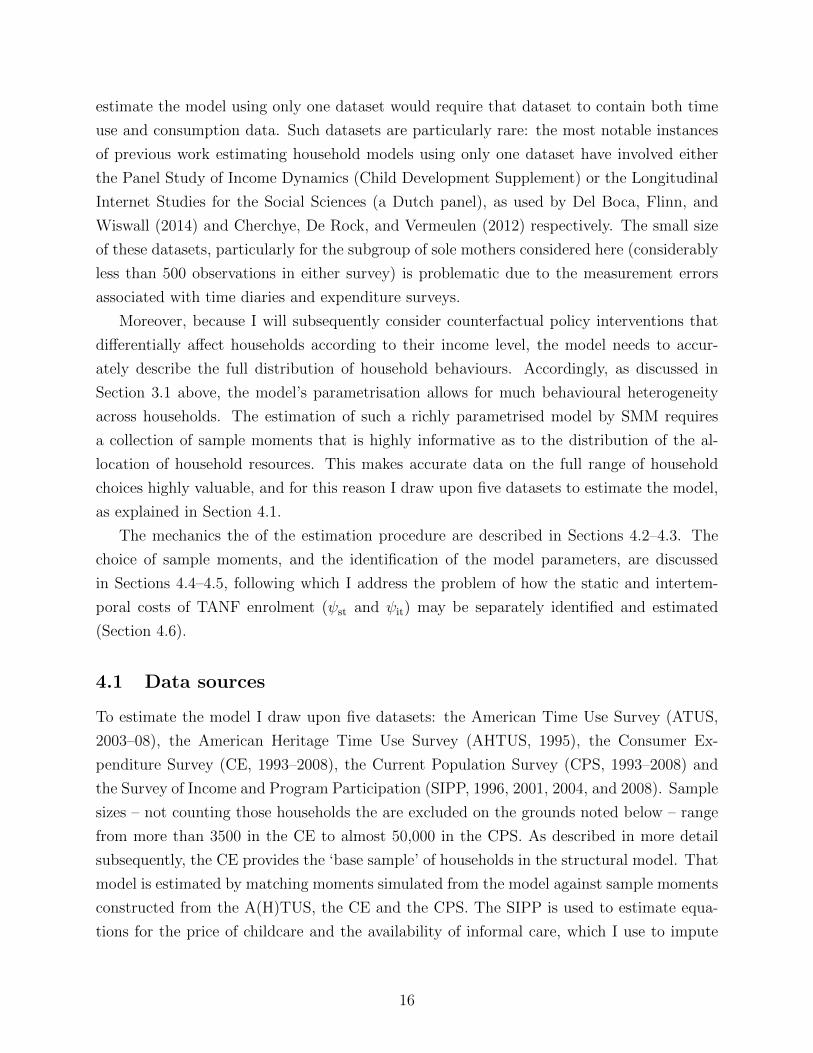
4.1 Data sources

To estimate the model I draw upon five datasets: the American Time Use Survey (ATUS,

2003–08), the American Heritage Time Use Survey (AHTUS, 1995), the Consumer Ex-

penditure Survey (CE, 1993–2008), the Current Population Survey (CPS, 1993–2008) and

the Survey of Income and Program Participation (SIPP, 1996, 2001, 2004, and 2008). Sample

sizes – not counting those households the are excluded on the grounds noted below – range

from more than 3500 in the CE to almost 50,000 in the CPS. As described in more detail

subsequently, the CE provides the ‘base sample’ of households in the structural model. That

model is estimated by matching moments simulated from the model against sample moments

constructed from the A(H)TUS, the CE and the CPS. The SIPP is used to estimate equa-

tions for the price of childcare and the availability of informal care, which I use to impute

16

Table 1: Descriptive statistics

ATUS CE CPS SIPP

(03-08) (93–08) (93–08) (96–08)∗

Household demographics

1 High school diploma (% of sample) 41 35 41 40Some tertiary education (%) 39 45 40 35

3 At least one child under 5 (%) 43 20 31 26More than one child (%) 42 44 41 29

Mother’s age (mean) 36 38 35 37

Labour supply

6 Paid work (hr/wk) 32 29 26Participation rate (%) 83 78 68

Wages (mean for participants; $/hr) 11.3

Weekly earnings ($/wk)

9 Mean 375

25th percentile 18050th percentile 32675th percentile 530

Intra-household allocation

13 Public consumption ($/wk) 251Private consumption ($/wk) 302

Non-labour income† ($/wk) 173

16 Time with children (hr/wk) 6.0Housework (hr/wk) 11.7

n 8484 3624 49676 2986

• Sample: as described in Section 4.1 (see also Appendix A). Sample period in parenthesis: 93–08 denotes1993–2008, etc. All dollar values are deflated to the year 2000. Statistics computed using inverse populationweights.

∗ SIPP only records data for the years 1996, 2001, 2004 and 2008.† Total non-durables consumption expenditure less after-tax earnings (constructed as per Section 4.4).

17

these missing childcare variables to households in the structural model (see the final part of

Section 4.2 below).

The A(H)TUS and the CE record time use and consumption expenditures at a much

finer level of detail than is needed for the broad categories (leisure, time with children,

etc.) to which the model refers. This has the considerable advantage of permitting me to

exercise discretion as to how different uses of time and expenditure, should be classified.

For example, I construct a measure of mother’s time with children that is focussed on those

activities that have been found to be be beneficial for child development, as discussed in

Section 4.4 below. Likewise, my measure of ‘public consumption’ includes expenditure on

goods that are not ‘public’ in the strict sense, such as food consumed at home, because it

is intended to capture all forms of expenditure that, together the mother’s housework, are

inputs to home production.

For all datasets, I restrict the sample by retaining only households in which: the mother

is aged 18–58 (or 25–58, for the CE); the mother is not self-employed or in the armed forces;

the household contains no more than one adult (i.e. one individual over the age of 18; this

restriction is not applied to the SIPP); the household’s residence is occupied by only one

family; the mother does not have a college degree (only 16 percent of sole mothers have a

college degree); and the mother’s hourly wage (if observed) lies in the range $2.50–$250 (in

2000 dollars). (See Appendix A for further details, including an explanation as to why a

different age range is used for the CE.)

Table 1 presents summary statistics for the ATUS, CE, CPS and SIPP samples. Here,

as is the case throughout this paper, all statistics are computed using the inverse population

weights provided by these surveys (normalised so that each year receives equal weight).

The results suggest that the samples are reasonably similar, particularly when allowance is

made for the different epochs to which they refer. The first two rows give the proportion

of the sample with only a high school diploma, and the proportion with a higher level of

educational attainment (i.e. a vocational qualification; recall that college-educated mothers

are excluded from the sample). Across all four datasets these figures differ by a maximum

of ten percentage points. Similarly, the mother’s average age does not vary much over the

three datasets, differing by only three years (see row 5). Female labour supply patterns are

also similar across the CE and CPS (see rows 6 and 7, cols 2 and 3, Table 1).

Table 1 also displays weekly (before-tax) earnings for sole mothers, drawn from the CE. In

this sample, 25 per cent of households earn under $180/wk, or $9,380/yr (in 2000 dollars),

while 50 per cent of households earn less than $16,900/yr. This compares to an official

poverty line of $11,250/yr for a one-child, sole-parent family, and $14,150/yr for a two-child,

sole-parent family.

18

4.2 Simulated method of moments

Marshallian demands Let Y = (y − s, wm, pu5, po5, au5, ao5) collect all the variables rel-

evant to the household’s budget constraint, and φ the household’s preference parameters.

(Though it would be tedious to enumerate φ in its entirety, it records the values of the

parameters δk, τ , ψst and ψit in (3.1), γm,c, γm,l, γq,l and ηm in (3.2), etc.) Recall that to

permit preference heterogeneity, some elements of φ are allowed to vary parametrically across

households. I accordingly write φ = φ(x, ξ; θ), where x denotes the household demographic

variables (age, education, race etc.), which I regard as exogenous, ξ the random disturbances

capturing the unobservable preference heterogeneity in the model, and θ the parameters in-

dexing φ(·). Thus, with δk = exp(x′δβδ + σδεδ) as per equation (3.5) above, εδ is an element

of ξ, and βδ a subvector of θ.

Since the feasible choice set C(y − s, d) depends on the whole of Y (not merely y − s),while each of u(·), K(·) and q(·) are parametrised by φ, the solution to (3.9) yields the

Marshallian demands

C = f(Y ;φ) = f [Y ;φ(x, ξ; θ)] = g(Y , x, ξ; θ) (4.1)

In principle, (4.1) should allow one to derive the density of C conditional on (Y , x), and

thence to estimate θ by maximum likelihood. In practice, there are two obstacles to this

route: (i) the evaluation of f requires solving the household’s problem numerically (no

analytical solution for the household’s problem is available), which makes calculation of the

likelihood challenging; and (ii) more significantly, as discussed in the introduction to this

section, the joint distribution of C is available in only a few small and – for our purposes –

unrepresentative datasets.

Construction of the moments For these reasons I estimate the model by simulated

method of moments. Since this does not require the recovery of the entire joint (conditional)

distribution of C, I am able to combine several datasets to build up an accurate picture

of the observed allocation of household resources, as described in more detail in Section 4.4

below. Regarding the selection of suitable moments, these could ordinarily be drawn from the

household’s first-order conditions: but with the present model, most of these would involve

non-separable functions of variables appearing in different datasets. I therefore instead

select the means, standard deviations and correlations of household choices, computed both

unconditionally and conditional on the household characteristics noted in Section 4.4 below.

More formally, the simulated moments are constructed by averaging across households

19

i ∈ 1, . . . , n and simulation draws s ∈ 1, . . . , S, as per

mn(θ) :=1

n

n∑i=1

πiS

S∑s=1

m[g(Y(i), x(i), ξ(is); θ);x(i)], (4.2)

where the πi’s are the inverse population weights from the CE, normalised so that∑n

i=1 πi =

n; m is a vector-valued transformation, chosen so as to deliver a vector of sample means of

the levels, squares and cross products of elements of Y ; and S is the number of simulation

draws. The final estimates are computed with S = 10. A further transformation puts the

moments into their required form (as means, standard deviations, and correlations); I write

this more compactly as µn(θ) = ϕ[mn(θ)].

An estimate of θ is then obtained by minimising the following criterion,

Qn(θ) =K∑k=1

(µnk(θ)− µnk)2

ω2k

= ‖µn(θ)− µn‖2W (4.3)

where µn = ϕ(mn) denotes the corresponding vector of sample moments, constructed from

data on household’s actual choices; W is a diagonal matrix with kth diagonal element ω−2k ;

and ‖x‖A := x′Ax. The inverse weights ω2k are computed from the estimated asymptotic

variance of the sample moment µnk; that is, as an estimate of ω2k in n1/2(µnk−µk)

d→ N [0, ω2k].

3

Although this does not correspond to the theoretically optimal weighting, it at least ensures

that sample moments from the same dataset are weighted proportionally to the precision

with which they are estimated, and renders Qn invariant to the units in which the households’

choices are measured.

The estimation procedure described by (4.2) and (4.3) has to be modified somewhat, to

take account of: (i) the imputation (via simulation) of those elements of Y that are missing

from the CE; and (ii) the introduction of additional moments, whose simulated counterparts

are computed on a slightly different basis from µn(θ), to ensure the identification of ψit. The

former is dealt with in Section 4.3; the latter is deferred to Section 4.6.

Computation of θ The minimisation of Qn is undertaken as follows. I first draw a large

number (20,000) of candidate values of θ, uniformly from a large, bounded subset of the

parameter space (chosen conservatively, so as to span all the economically plausible values

of the parameters). I evaluate Qn at each of these points, and retain θ(k)’s corresponding

3Note that ω2k does not depend on the size of the sample used to estimate µnk: were I to instead

weight the moments by their approximate finite-sample variances ω2k/n, I would grossly over-weight moments

constructed from the CPS, which has a much larger sample size than either the CE or the A(H)TUS (seeTable 1).

20

to the 1000 smallest values of Qn(θ(k)) thus obtained. From each of these points, I run 300

iterations of a Gauss-Newton optimisation routine, and then retain the 500 best-performing

optimisations, following which I run a further 600 iterations of Gauss-Newton. (I use the

implementation of the Gauss-Newton routine provided by version 10 of the Artelys Knitro

software package.) I then take the best 100 points remaining, and iterate Gauss-Newton from

these until convergence. The estimates reported in this paper correspond to the parameters

delivering the minimum value of Qn achieved by this algorithm. (Four optimisers converged

to this point of the parameter space; others terminated at higher values of Qn.) As a check

on my results, I also ran ten independent simulated annealing chains, each of 1 million draws

in length, starting from the ten best randomly-sampled values (as drawn at the first stage of

the preceding algorithm), followed by a Gauss-Newton optimisation, iterated to convergence:

but in no case did this beat the estimates obtained by the preceding algorithm.

Inference Under the assumption that the model is correctly specified (with paramet-

ers θ0), and the number of simulation draws S is fixed as n → ∞, standard results on

minimum-distance-type estimators (see e.g. Gourieroux, Monfort, and Renault, 1993) imply

that n1/2(θ − θ0)d→ N [0, V ], where

V = (D′WD)−1D′WΣWD(D′WD)−1 (4.4)

forD = ∂θµ(θ0) the Jacobian of µ(·) = plim µn(·) at θ0, Σ the limiting variance of n1/2[µn(θ0)−µn], and W = plim W . (Note that V depends on S through Σ.) The estimation of V requires

estimators for D and Σ. D can be estimated by numerically differentiating µn with respect

to θ at θ. The estimation of Σ is somewhat complicated by the use of multiple datasets, and

so a discussion of this is deferred to Appendix B.3. (Note that inferences based on V ignore

the additional variability introduced by the imputation procedure described in the following

section.)

4.3 Imputation (via simulation) of missing variables

Recall that I use the CE (1993–2008) as to construct the ‘base sample’ of households in the

model: this provides me with data on x, wm (for most households), and y − s; this last

being computed as the excess of total consumption expenditures (including childcare) over

after-tax earnings (see (3.7) above). However, wm is not observed for working mothers, while

childcare prices and the availability of informal care, (pu5, po5, au5, ao5), are not observed for

any household in the CE. I therefore estimate a collection of models that allow values of these

missing variables to be simulated, prior to estimating the structural model. To describe these,

21

let each of xm, xy, xp, and xa denote subvectors of the household demographic variables x;

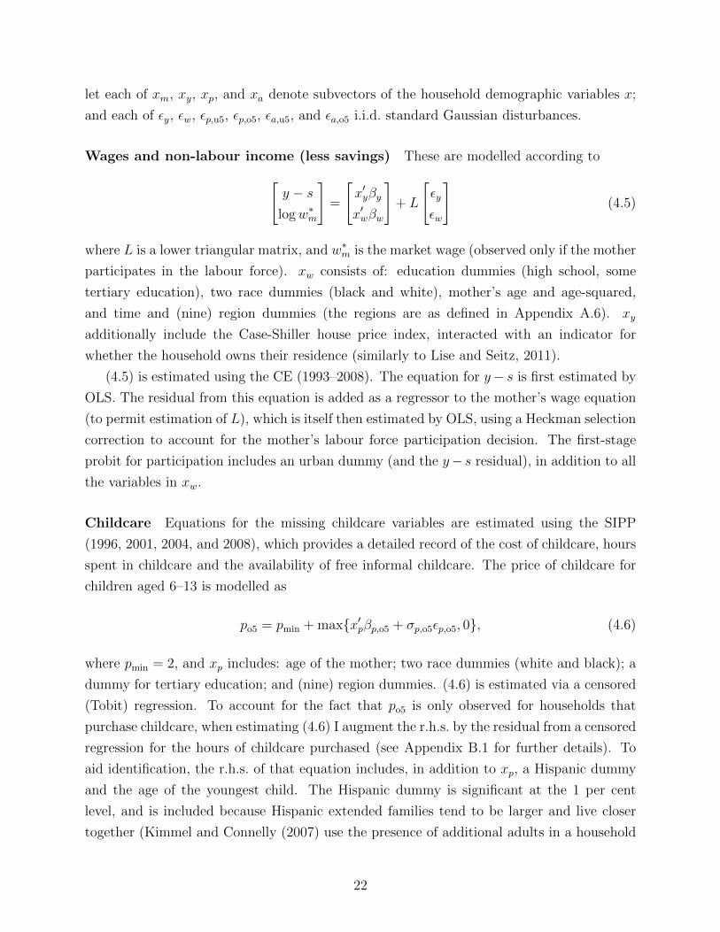
and each of εy, εw, εp,u5, εp,o5, εa,u5, and εa,o5 i.i.d. standard Gaussian disturbances.

Wages and non-labour income (less savings) These are modelled according to[y − s

logw∗m

]=

[x′yβy

x′wβw

]+ L

[εy

εw

](4.5)

where L is a lower triangular matrix, and w∗m is the market wage (observed only if the mother

participates in the labour force). xw consists of: education dummies (high school, some

tertiary education), two race dummies (black and white), mother’s age and age-squared,

and time and (nine) region dummies (the regions are as defined in Appendix A.6). xy

additionally include the Case-Shiller house price index, interacted with an indicator for

whether the household owns their residence (similarly to Lise and Seitz, 2011).

(4.5) is estimated using the CE (1993–2008). The equation for y− s is first estimated by

OLS. The residual from this equation is added as a regressor to the mother’s wage equation

(to permit estimation of L), which is itself then estimated by OLS, using a Heckman selection

correction to account for the mother’s labour force participation decision. The first-stage

probit for participation includes an urban dummy (and the y− s residual), in addition to all

the variables in xw.

Childcare Equations for the missing childcare variables are estimated using the SIPP

(1996, 2001, 2004, and 2008), which provides a detailed record of the cost of childcare, hours

spent in childcare and the availability of free informal childcare. The price of childcare for

children aged 6–13 is modelled as

po5 = pmin + maxx′pβp,o5 + σp,o5εp,o5, 0, (4.6)

where pmin = 2, and xp includes: age of the mother; two race dummies (white and black); a

dummy for tertiary education; and (nine) region dummies. (4.6) is estimated via a censored

(Tobit) regression. To account for the fact that po5 is only observed for households that

purchase childcare, when estimating (4.6) I augment the r.h.s. by the residual from a censored

regression for the hours of childcare purchased (see Appendix B.1 for further details). To

aid identification, the r.h.s. of that equation includes, in addition to xp, a Hispanic dummy

and the age of the youngest child. The Hispanic dummy is significant at the 1 per cent

level, and is included because Hispanic extended families tend to be larger and live closer

together (Kimmel and Connelly (2007) use the presence of additional adults in a household

22

for a similar purpose).

The hours of free informal childcare available to the household (i.e. care provided by

relatives) for children aged 6–13 are given by

ao5 = maxx′aβa,o5 + σa,o5εa,o5, 0, (4.7)

where xa includes the same variables as xp, and additionally an indicator for whether the

family owns their residence. ao5 is subjected to further censoring and sample selection, since

only minao5, hm is observed, and that only if hm > 0. Accordingly, I estimate (4.7) by a

doubly-censored regression regression, with 0 as the left and hm as the right censor point

(see Appendix B.1). To control for the right censoring and sample selection, I augment the

r.h.s. of (4.7) with the residual from an estimated censored regression for hours worked (the

r.h.s. of that equation includes xa, a Hispanic dummy and the age of the youngest child).

Analogous equations to (4.6) and (4.7) hold for children aged 0–5, and are estimated in the

same way (see Appendix B.1).

Imputation via simulation Estimates of the parameters of (4.5)–(4.7) are reported in

Appendix C.1. Given these estimates, and data on (y − s)(i) and x(i) for the ith household,

I can use these equations to simulate values for those elements of Y that are missing, by

drawing values for the disturbances (εw, εp,u5, εp,o5, εa,u5, εa,o5) from a multivariate standard

normal. (Since y − s is always observed, the residual εy from equation (4.5) is used to

construct a simulated value for wm.) Let Y(is) denote the simulated values obtained for

the sth simulation applied of the ith household, where Y(is) records the observed values of

(y − s)(i) and – when these are available – wm,(i). Then the simulated moments at θ can be

written as

mn(θ) :=1

n

n∑i=1

πiS

S∑s=1

m[g(Y(is), x(i), ξ(is); θ);x(i)], (4.8)

so that the only difference between the preceding and equation (4.2) is that the (partially

unobserved) Y(i) has been replaced by the (partially simulated) Y(is).

4.4 Sample moments: selection and construction

As noted above, the ‘base sample’ of households in the structural model is drawn from the

CE (1993–2008); this is used to construct simulated moments for a given value of θ. To

construct the sample moments against which these are to be matched, I draw upon four

datasets: the ATUS (2003–08) and the AHTUS (1995) for data on mother’s time use; the

CE (1993–2008) for household consumption expenditures, wages, and non-labour income;

23

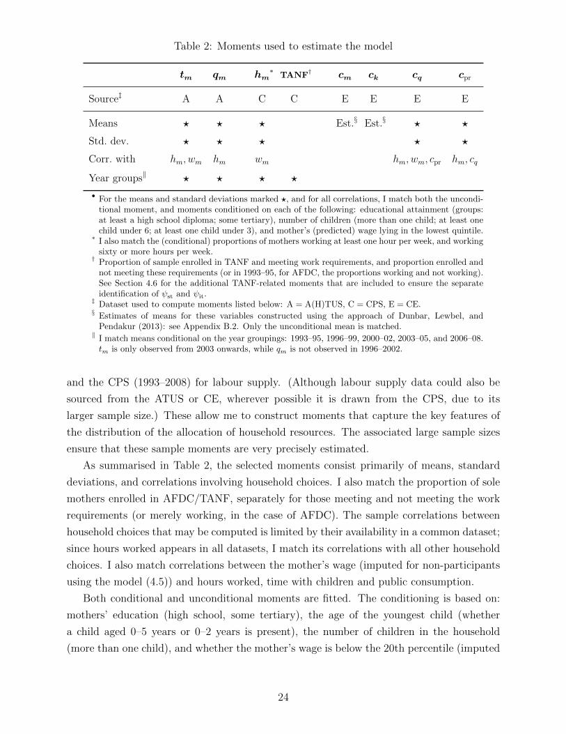
Table 2: Moments used to estimate the model

tm qm hm∗

TANF† cm ck cq cpr

Source‡ A A C C E E E E

Means ? ? ? Est.§ Est.§ ? ?

Std. dev. ? ? ? ? ?

Corr. with hm, wm hm wm hm, wm, cpr hm, cq

Year groups‖ ? ? ? ?

• For the means and standard deviations marked ?, and for all correlations, I match both the uncondi-tional moment, and moments conditioned on each of the following: educational attainment (groups:at least a high school diploma; some tertiary), number of children (more than one child; at least onechild under 6; at least one child under 3), and mother’s (predicted) wage lying in the lowest quintile.

∗ I also match the (conditional) proportions of mothers working at least one hour per week, and workingsixty or more hours per week.

† Proportion of sample enrolled in TANF and meeting work requirements, and proportion enrolled andnot meeting these requirements (or in 1993–95, for AFDC, the proportions working and not working).See Section 4.6 for the additional TANF-related moments that are included to ensure the separateidentification of ψst and ψit.

‡ Dataset used to compute moments listed below: A = A(H)TUS, C = CPS, E = CE.§ Estimates of means for these variables constructed using the approach of Dunbar, Lewbel, and

Pendakur (2013): see Appendix B.2. Only the unconditional mean is matched.‖ I match means conditional on the year groupings: 1993–95, 1996–99, 2000–02, 2003–05, and 2006–08.tm is only observed from 2003 onwards, while qm is not observed in 1996–2002.

and the CPS (1993–2008) for labour supply. (Although labour supply data could also be

sourced from the ATUS or CE, wherever possible it is drawn from the CPS, due to its

larger sample size.) These allow me to construct moments that capture the key features of

the distribution of the allocation of household resources. The associated large sample sizes

ensure that these sample moments are very precisely estimated.

As summarised in Table 2, the selected moments consist primarily of means, standard

deviations, and correlations involving household choices. I also match the proportion of sole

mothers enrolled in AFDC/TANF, separately for those meeting and not meeting the work

requirements (or merely working, in the case of AFDC). The sample correlations between

household choices that may be computed is limited by their availability in a common dataset;

since hours worked appears in all datasets, I match its correlations with all other household

choices. I also match correlations between the mother’s wage (imputed for non-participants

using the model (4.5)) and hours worked, time with children and public consumption.

Both conditional and unconditional moments are fitted. The conditioning is based on:

mothers’ education (high school, some tertiary), the age of the youngest child (whether

a child aged 0–5 years or 0–2 years is present), the number of children in the household

(more than one child), and whether the mother’s wage is below the 20th percentile (imputed

24

wage for non-participants). Conditioning on this final group is motivated by low-income

households being the most likely to receive government assistance, and as such being of

particular relevance to this paper. For those variables indicated in the table, I also condition

on the following year groups: 1993–95, 1996–99, 2000–02, 2003–05, and 2006–08.

Mothers’ time use Moments for mothers’ time use include the (conditional) means and

standard deviations of hours worked, housework, and time with children (leisure is excluded,

since all time uses must sum to 105 hr/wk).

The ATUS (2003–08) provides a single 24-hour time diary for each mother on a randomly

selected day of the week. These time diaries are used to construct measures of parents’ time

with children, and time spent in housework. (The ATUS separately records the number of

hours worked per week.) My measure of time with children is an aggregate of time spent in

activities that have been found beneficial for child development, including: reading to chil-

dren (Scarborough and Dobrich, 1994), talking with parents (Tamis-LeMonda, Bornstein,

and Baumwell, 2001), mealtime conversation (Snow and Beals, 2006), and novel experi-

ences and places (Phillips, 2011). The AHTUS (1995) provides similar time diary data, but

the significant differences in the classification of activities across the two surveys prevents

the construction of a comparable measure of parents’ time with children. I therefore only

draw data on time spent in housework from the AHTUS. (Further details are provided in

Appendix A.1.)

A shortcoming of this data is that the time diaries only record activities during a 24-

hour window, whereas I am interested in average behaviour over the course of a week.

First moments (and certain cross-correlations) involving time use may still be consistently

estimated from such time-diary data, but measures of variability will be upwardly biased.

I accordingly adjust the sample standard deviations computed for these variables, using

estimates of this bias computed from another dataset (from the Netherlands) which provides

time diaries for an entire week for each respondent (see Appendix A.1 for details).

Consumption expenditures I match the (conditional) means and standard deviations of

public and total private consumption expenditures, measures of which are constructed from

the CE. Public consumption includes such categories as food, utilities, mortgage interest, and

rent (see Appendix A.3). Private consumption is computed as total household expenditure

less public consumption and childcare costs.

Two additional moments help to calibrate the breakdown of private consumption between

household members. Since it is only possible to unambiguously assign expenditures on a few

commodities recorded in the CE (e.g. clothing) to either the mother or her children, I use

25

the procedure developed by Dunbar, Lewbel, and Pendakur (2013) to infer the average

breakdown of total private consumption expenditures, between mothers and children (see

Appendix B.2 for further details). This provides me with estimates of the unconditional

means of mother’s and children’s private consumption, which are matched by the estima-

tion procedure; note that no conditional means are matched, so this only contributes two

additional moments (out of a total of 173).

4.5 Identification of structural parameters

Two questions pertinent to the identification of the structural parameters are: (i) what exo-

genous variation is present in the sample that might help to identify those parameters; and,

since those parameters are to be estimated by SMM, (ii) do the moments provide a suffi-

ciently rich description of the data to capture the principal trade-offs faced by households?

I give a brief discussion of both these questions here, before providing a further numerical

analysis of parameter identification in Section 5.4 below.

The evolution of tax and welfare policies over the sample epoch provides the main source

of exogenous variation in households’ budgets. Changes to these policies have clearly affected

household behaviour: for instance, the reduced generosity of TANF relative to AFDC has

likely contributed to the marked increase in the time that sole mothers have spent in paid

work, instead of in housework, since 1996 (recall Section 2.2 above). The moments matched

by the estimation procedure include the means of certain household choices conditional on

each of five subperiods, thereby capturing these aggregate trends. As shown in Section 5.2

below, the model achieves a good fit to these trends, suggesting that it accurately predicts

households’ responses to (exogenous) variation in the tax and welfare system.

Even stronger evidence for this comes from the external validation exercise performed in

Section 5.3 below. TANF greatly widened regional disparities in the generosity of welfare

payments, by devolving much of the responsibility for welfare provision to the states (see

Section 2.2 above). Although none of the moments used to estimate the model condition

on location – and thus omit any region-specific trends in household resource allocation that

might have resulted from this policy variation – I show below that the estimated model is

able to match region-specific trends in household time use and consumption over 1993–2008

with a high degree of accuracy. I interpret the model’s success in capturing how households

respond to changes to welfare policies as implying that variation in these policies must be

highly influential in pinning down the values of the estimated parameters.

With respect to the second aspect to identification, it should first be noted that in

contrast to much of the prior empirical literature that estimates intra-household models

26

using only consumption data (Apps and Rees, 1996; Lise and Seitz, 2011; Dunbar, Lewbel,

and Pendakur, 2013), I have at my disposal both time use and consumption data, which

taken together provide a far richer description of the allocation of household resources.

The correlations among household choices, and between those choices and wages, ought

to be particularly informative as to the trade-offs households face when deciding between

alternative uses of those resources. Although it is not possible for me to include all such

correlations – because not all variables appear in a common dataset – I am able to include

correlations between all household choices and hours worked.

4.6 Identifying the TANF enrolment disutilities

While the total disutility ψ = ψst + ψit associated with TANF enrolment is identified from

the observed enrolment rates (conditional on the year groups indicated), this does permit the

separate recovery of its components, ψst and ψit. Recall that ψit captures the ‘intertemporal’

cost of enrolling in TANF, due to lifetime limits. Solving the model with ψit = 0 thus yields

the enrolment rate, implied by the model’s other parameters, that would counterfactually

obtain if lifetime limits were absent. I propose to match this to a sample estimate of the

proportion of households would enrol in TANF, in the absence of lifetime limits. ψit (and

thus also ψst = ψ − ψit) may then be identified from the estimated effect of lifetime limits

on TANF enrolment.

Several papers have previously estimated this effect: here I follow the approach of Grogger

and Michalopoulos (2003). They exploit the fact that when TANF was introduced, lifetime

limits were not binding on households in which all children were aged over 12 – whereas

all other households were to some extent constrained by these limits. More formally, their

approach involves estimating the following probit regression for TANF enrolment

d = 1x′dβd + β1z1 + β2z2 + ε > 0, (4.9)

where: d = 1 if the mother enrols in TANF; ε ∼ N [0, 1]; xd is a vector of controls; and z1

and z2 are dummy variables, with z1 = 1 for a mother who was never subject to time limits

(because her youngest child was over 12 when time limits were introduced to her state), and

z2 = 1 for a mother who was only partially exposed to time limits (because her youngest

child was born before time limits were introduced). I control for the age composition of the

children in the household, by including dummies for the presence of children aged 0–2, 3–5,

and 6–12 in xd. I also include dummies for the periods 1996–99, 2000–02, 2003–05, 2006–08,

to allow the disutility from enrolling in TANF to change over time. xd additionally includes:

the mother’s age and age-squared; race dummies (white and black); a dummy for whether

27

there is only one child in the household; a dummy for whether the mother has some tertiary

education; and nine region effects (for the regions given in Appendix A.6).

Across 1996 to 2008, an average of 18 per cent of sole mothers in the CPS were enrolled in

TANF. Using the procedure outlined above, this figure would rise to 22 per cent if time-limits

were eliminated.

The parameters of (4.9) are estimated using the CPS (see Table 10 in Appendix C.2).

Conditional on xd, the estimated probability that a household that would enrol in TANF

in the absence of time limits is given by Φ(x′dβd + β1). Averaging this over the entire CPS

sample (1996–2008) gives an implied TANF enrolment probability in the absence of lifetime

limits of 22 per cent, as compared with an observed enrolment rate of 18 per cent. To

construct the additional sample moments νn that are matched by the estimation procedure,

I compute sample averages of Φ(x′dβd + β1), both unconditionally and conditional on the

presence of: a child aged 0–5, and two or more children. Doing this for each of time periods

1996–99, 2000–02, 2003–05 and 2006–08 yields a total of 12 additional moments.

To construct the simulated moments that correspond to νn, I partition the parameters

of the structural model as θ = (ϑ, ψit), so that solving the model with ψit = 0 yields the

enrolment rates that would obtain under ϑ, in the absence of lifetime limits. Let νn(ϑ) denote

the vector of simulated moments thus computed. The overall criterion that I minimise to

estimate the structural parameters is (4.3) augmented by the squared weighted distance

between νn and νn(ϑ), i.e.

Q′n(ϑ, ψit) = ‖µn(ϑ, ψit)− µn‖2W + ‖νn(ϑ)− νn‖2

V

where V is a diagonal weight matrix whose elements are computed on the same basis as

those of W (see Section 4.2 above).

5 Estimates and model fit

In this section I demonstrate that the model performs well according to three different

criteria. Firstly, the mother’s labour supply elasticities are within the range of those obtained

in previous studies (Section 5.1). Secondly, the model achieves a good (in-sample) fit to the

moments used in estimation (Section 5.2). In particular, the model is able to replicate those

aggregate trends in household behaviour that were discussed in Section 2.2 above.

Thirdly, the model is able to match ‘out-of-sample’ variation in household choices: that

is, variation observed during the sample period, but which is not directly targeted by the

estimation procedure. To this end, I show that observed region-specific trends in household

28

choices over the sample period correlate closely with those predicted by the model. Such

geographical variation is of particular interest, as it has doubtless been influenced by the

manner in which TANF extended considerably greater freedom to states in setting the para-

meters of their welfare programmes (recall Section 2.1 above). The good performance of the

model in this respect lends greater credibility to the counterfactual exercises subsequently

conducted in Section 6, which involve changes to welfare policy different from those observed

historically.

Finally, I also investigate empirically how different subsets of the selected moments con-

tribute to the identification of the model’s parameters, to complement the heuristic discussion

of parameter identification in Section 4.4 above (see Section 5.4). I quantify this by comput-

ing how the precision of the parameter estimates, in terms of their estimated standard errors,

would be affected if certain moments were ignored by the estimation procedure. Consist-

ent with the heuristic discussion of identification (see Section 4.4 above), time-use moments

and correlations among household choices significantly strengthen the identification of the

structural parameters.

5.1 Parameter estimates

The average values of the behavioural parameters implied by the estimates, conditional on

certain household characteristics, are displayed in Table 3. For the estimated CES utility and

production functions, I report the (more readily interpretable) elasticities of substitution ςi

rather than the corresponding curvature parameters ηi; the two are related via ςi = 1/(1−ηi).As discussed in Section 3.1 above, the model allows for considerable heterogeneity (both

observable and unobservable) in household preferences. The number of underlying structural

parameters is accordingly rather large (48), and so a complete listing of their estimates is

deferred to Appendix C.3. (Estimates of the parameters for the models used to impute

missing variables are given in Appendix C.1.)

The estimates indicate that the children’s utility function places a relatively large weight

on the public good, with γk,q = 0.42 as compared with γm,q = 0.18 for mothers (see row 9).

Thus children significantly benefit from expenditure on housing (cq includes imputed rents),

home cooked meals, and having a clean and tidy house. In households with children aged

0–5, the children’s utility places a higher weight on the mother’s time with children, and the

degree of substitutability between inputs is lower than it is on average (see rows 8 and 12).

In home production, the elasticity of substitution between maternal time and consump-

tion is estimated to be 1.07 (row 13, col 1). This is slightly higher than the average elasticity

of substitution estimated for inputs into the child utility function, at 0.83 (row 11, col 2).

29

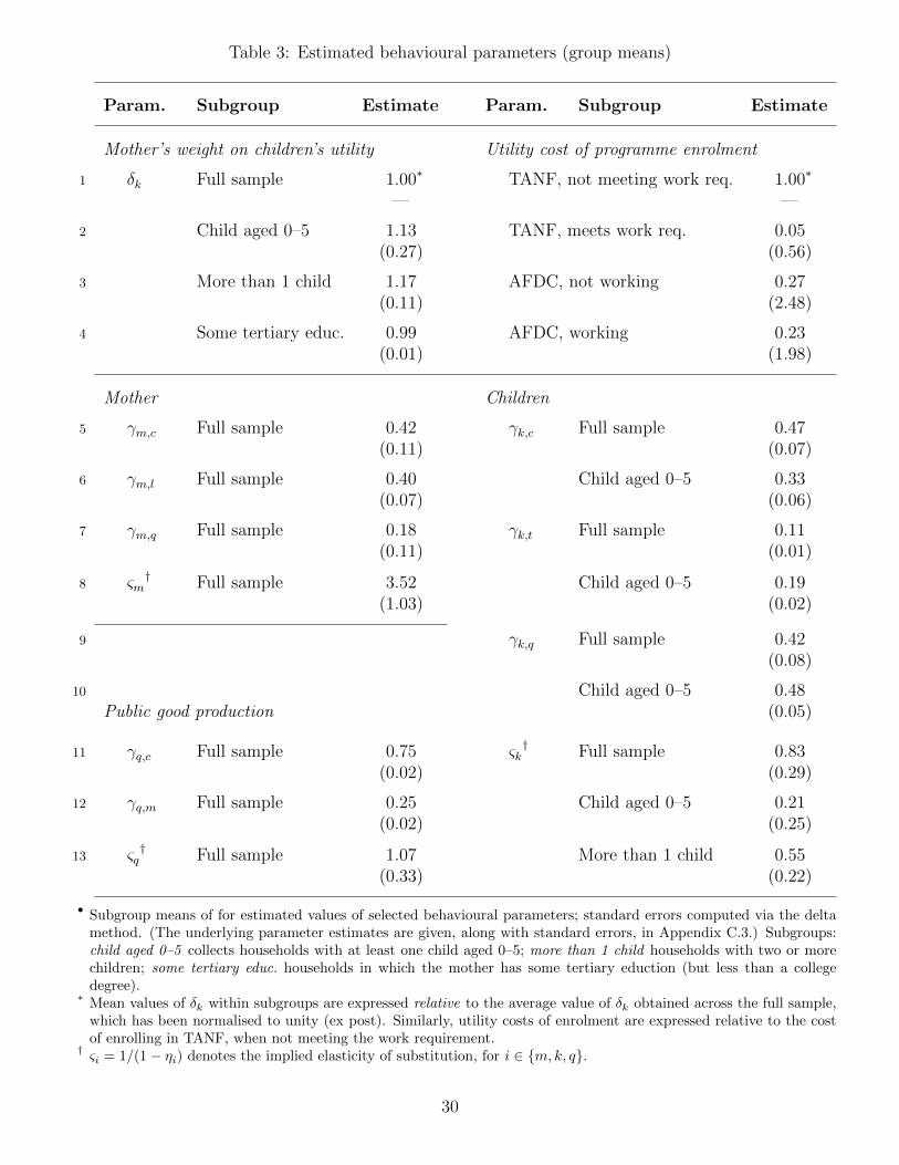
Table 3: Estimated behavioural parameters (group means)

Param. Subgroup Estimate Param. Subgroup Estimate

Mother’s weight on children’s utility Utility cost of programme enrolment

1 δk Full sample 1.00∗ TANF, not meeting work req. 1.00∗

— —

2 Child aged 0–5 1.13 TANF, meets work req. 0.05(0.27) (0.56)

3 More than 1 child 1.17 AFDC, not working 0.27(0.11) (2.48)

4 Some tertiary educ. 0.99 AFDC, working 0.23(0.01) (1.98)

Mother Children

5 γm,c Full sample 0.42 γk,c Full sample 0.47(0.11) (0.07)

6 γm,l Full sample 0.40 Child aged 0–5 0.33(0.07) (0.06)

7 γm,q Full sample 0.18 γk,t Full sample 0.11(0.11) (0.01)

8 ςm† Full sample 3.52 Child aged 0–5 0.19

(1.03) (0.02)

9 γk,q Full sample 0.42(0.08)

10 Child aged 0–5 0.48Public good production (0.05)

11 γq,c Full sample 0.75 ςk† Full sample 0.83

(0.02) (0.29)

12 γq,m Full sample 0.25 Child aged 0–5 0.21(0.02) (0.25)

13 ςq† Full sample 1.07 More than 1 child 0.55

(0.33) (0.22)

• Subgroup means of for estimated values of selected behavioural parameters; standard errors computed via the deltamethod. (The underlying parameter estimates are given, along with standard errors, in Appendix C.3.) Subgroups:child aged 0–5 collects households with at least one child aged 0–5; more than 1 child households with two or morechildren; some tertiary educ. households in which the mother has some tertiary eduction (but less than a collegedegree).

∗ Mean values of δk within subgroups are expressed relative to the average value of δk obtained across the full sample,which has been normalised to unity (ex post). Similarly, utility costs of enrolment are expressed relative to the costof enrolling in TANF, when not meeting the work requirement.

† ςi = 1/(1− ηi) denotes the implied elasticity of substitution, for i ∈ m, k, q.

30

It is somewhat lower than the estimates of 1.25, 2.44, and 1.80 obtained respectively by

McGrattan, Rogerson, and Wright (1997), Chang and Schorfheide (2003) and Aguiar and

Hurst (2007); however, it should be noted that those estimates are not exactly comparable

with my own, since they are based on a sample of households that includes both sole mothers

and married couples.

The disutility from TANF enrolment is estimated to be significantly higher when work

requirements are met, than when they are not (see rows 1–2, col 2). Indeed, the estimated

disutility from enrolment for those meeting the work requirements is so low as to have ap-

parently little effect on enrolment: the model predicts that if this disutility were eliminated,

the proportion of the sample enrolled in TANF and meeting work requirements, averaged

over 1996–2008, would rise by only 0.9 percentage points to 3.4 per cent. For AFDC, on the

other hand, the estimated disutility suffered by enrollees differs little between those working

(0.23) and those not (0.27; see rows 3–4, col 2). These differences between the estimates for

two programmes are entirely consistent with TANF more heavily sanctioning those who fail

to meet its work requirements.

Maternal labour supply elasticity I compute the aggregate wage elasticity implied by

these estimates by: (i) incrementing the wage of every household (including non-participants)

in the structural model by $1/hr (in 2000 dollars); (ii) solving each household’s optimisation

problem under this counterfactually higher wage, to obtain their hours worked hm,i(w∗m,i);

and then (iii) computing the ratio of the percentage changes in the model averages of hours

worked and the hourly wage, which can be rewritten as

∆h

h· w

∆w=

1n

∑ni=1 πi[hm,i(wm,i + 1)− hm,i(wm,i)]

1n

∑ni=1 πihm,i(wm,i)

·1n

∑ni=1 πiwm,i

1n

∑ni=1 πi · 1

(5.1)

This yields an estimated elasticity of 0.67; the elasticity at the intensive margin is 0.27.

(This is computed by restricting the averages on the r.h.s. of equation (5.1) to the subgroup

of mothers who work in the baseline.) These estimates are similar to those obtained for sole

mothers by (see Blundell, Costa Dias, Meghir, and Shaw, 2016).

5.2 Model fit: in-sample performance

Aggregate trends in household behaviour As discussed in Section 2.2 above, house-

hold behaviour changed systematically over 1993–2008 – possibly in response to the intro-

duction of TANF – with in particular a very discernible shift from housework into market

work (see also Meyer and Sullivan, 2008). Plots of observed and model-implied paths for

31

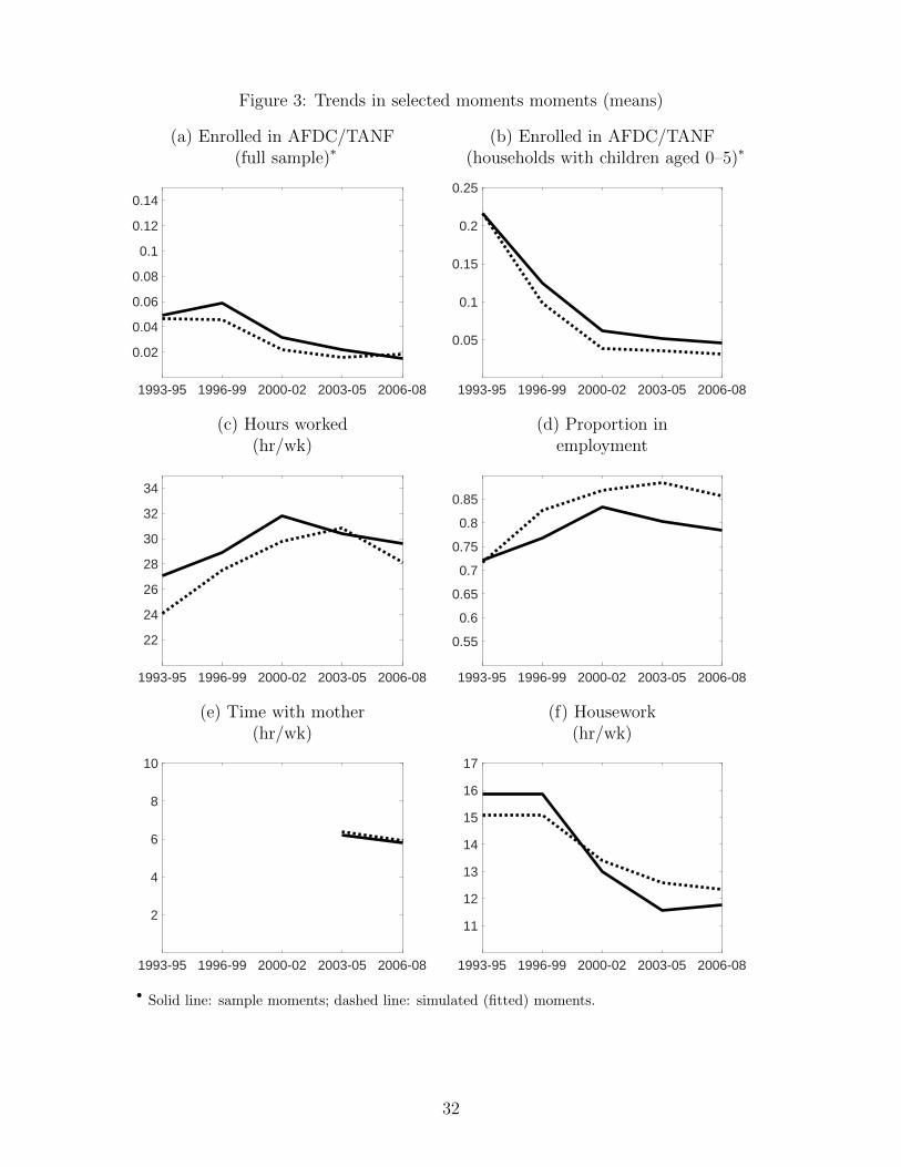
Figure 3: Trends in selected moments moments (means)

(a) Enrolled in AFDC/TANF (b) Enrolled in AFDC/TANF(full sample)∗ (households with children aged 0–5)∗

1993-95 1996-99 2000-02 2003-05 2006-08

0.02

0.04

0.06

0.08

0.1

0.12

0.14

1993-95 1996-99 2000-02 2003-05 2006-08

0.05

0.1

0.15

0.2

0.25

(c) Hours worked (d) Proportion in(hr/wk) employment

1993-95 1996-99 2000-02 2003-05 2006-08

22

24

26

28

30

32

34

1993-95 1996-99 2000-02 2003-05 2006-08

0.55

0.6

0.65

0.7

0.75

0.8

0.85

(e) Time with mother (f) Housework(hr/wk) (hr/wk)

1993-95 1996-99 2000-02 2003-05 2006-08

2

4

6

8

10

1993-95 1996-99 2000-02 2003-05 2006-08

11

12

13

14

15

16

17

• Solid line: sample moments; dashed line: simulated (fitted) moments.

32

these selected household choices are displayed in Figure 3. (Recall from Section 4.4 that

the means of these choices, conditional on each of the year groups displayed, are among the

moments used for SMM.)

The model fits the trend decline in the AFDC/TANF enrolment rate both overall, and

for households with children aged 0–5 (panels (a)–(b)). Regarding maternal time use, the

model is able to match most of the increase in hours worked over 1993–2002, although hours

worked is underestimated in the earlier part of the sample by about 3 hr/wk. Labour force

participation is systematically overestimated by around 5 percentage points. The model also

matches around three-quarters of the 4 hr/wk decline in housework over 1993–2008. Thus

the model is able to account for the main trends in household behaviour since the introduc-

tion of TANF, which lends greater credibility to the counterfactual exercises subsequently

performed.

First and second moments First and second moments for mothers’ choices appear in

Table 4: both simulated and sample moments are reported (standard errors of the sample

moments in parentheses). On the whole, these moments are fit reasonably well. As noted in

Section 4.4 above, I have included moments that condition on mothers’ wages being below the

20th percentile, because these households are of particular concern in this paper, being the

most likely to receive government assistance. The model fits these moments well, with each

simulated moment lying within (or very nearly within) the 95 per cent confidence interval

for the corresponding sample moment in all cases (see rows 2 and 9).

Time use First and second moments for mothers’ time use appear in columns 1–6 of

Table 4.

The model closely fits all moments describing mothers’ time with children (see cols 1–2).

The unconditional simulated mean is within one standard deviation of the sample mean,

and much of the variation across subgroups is reproduced by the model, with all the model-

implied conditional means lying within two standard deviations of their sample counterparts

(rows 2–7, cols 1–2). Housework moments (cols 3–4) are fit slightly less well. The uncon-

ditional mean of time spent in housework is over-estimated by one hour per week, and the

model predicts there to be greater variation in housework time across subgroups than is

actually present in the sample.

Although the unconditional mean of hours worked is fit well, the model does not fully

capture the observed covariation of labour supply with observables (cols 5–6). For subgroups

in which hours worked is less than the unconditional mean, the model somewhat exaggerates

the difference between the conditional and unconditional means. For example, for households

33

Table 4: Time-use and consumption moments

Time w/child. Housework Hours worked Public cons. Private cons.(hr/wk) (hr/wk) (hr/wk) ($/wk) ($/wk)

Siml. Smpl. Siml. Smpl. Siml. Smpl. Siml. Smpl. Siml. Smpl.

1 2 3 4 5 6 7 8 9 10

Mean

1 Full Sample 6.16 6.00 12.48 11.66 28.66 29.46 252.96 250.60 302.65 301.67(0.21) (0.30) (0.09) (3.50) (5.60)

2 Wage in lowest 7.45 7.83 11.72 12.27 22.60 24.71 219.99 211.22 237.46 218.18quintile (0.46) (0.61) (1.37) (5.76) (8.79)

Education

3 High school (at least) 6.09 6.14 13.68 12.06 29.27 30.07 260.42 241.83 297.08 297.92(0.34) (0.51) (0.15) (4.74) (9.34)

4 Some tertiary 5.94 6.05 11.71 10.80 28.91 33.09 260.30 272.02 334.38 340.77(0.31) (0.39) (0.13) (5.92) (8.67)

Family structure

5 Children under 5 10.35 9.60 8.42 12.00 22.13 26.28 235.55 236.27 268.73 279.71(0.41) (0.48) (0.18) (7.15) (13.6)

6 Children under 2 10.08 10.86 8.91 11.95 225.41 220.56 252.59 264.63(0.58) (0.62) (9.91) (20.4)

7 More than 1 child 7.43 6.97 12.87 11.88 25.70 28.34 244.84 256.40 316.85 302.90(0.34) (0.47) (0.15) (5.53) (9.12)

Standard deviation

8 Full Sample 4.53 4.49 7.75 7.66 18.52 17.55 112.81 103.90 167.49 171.66(0.09) (0.12) (0.05) (5.02) (5.35)

9 Wage in lowest 5.30 4.91 7.12 7.89 ??? ??? 96.09 86.00 130.90 123.66quintile (0.18) (0.27) ??? (6.35) (8.99)

Education

10 High school (at least) 3.86 4.41 7.48 7.63 18.79 17.06 111.26 90.71 166.25 169.27(0.14) (0.16) (0.09) (4.90) (9.46)

11 Some tertiary 4.49 4.51 7.72 7.33 17.97 15.57 118.02 113.57 172.51 177.25(0.14) (0.17) (0.11) (8.86) (7.79)

Family structure

12 Children under 5 5.11 5.08 7.53 7.65 17.41 18.09 114.88 96.39 127.80 169.52(0.13) (0.18) (0.08) (5.80) (11.8)

13 Children under 2 4.81 5.17 7.32 7.69 110.53 88.45 126.75 169.88(0.18) (0.23) (7.89) (24.4)

14 More than 1 child 5.30 4.99 8.67 7.65 17.72 17.77 110.11 107.89 167.11 178.94(0.15) (0.21) (0.08) (9.45) (8.65)

• Simulated moments (Siml.) corresponding to the model parameter estimates, and sample moments (Smpl.) computed from the data. Standarderrors of sample moments in parentheses. All dollar values are in year 2000 dollars.

34

with wages below the 20th percentile, average hours worked is under-predicted by two hours,

as compared with 0.8 hours overall.

The standard deviations are also fit well, with the standard deviation of hours worked

slightly over-predicted (rows 8–14, cols 5–6). There is little variation in the standard devi-

ation of the time-use moments across the subgroups.

Consumption The model’s fit to the means and standard deviations of public and private

consumption is reported in columns 7–10 of Table 4. Both unconditional means are fit closely

(see row 1). The model is successfully matches the observed variation in consumption ex-

penditures across subgroups. For example, the $39/wk difference between the unconditional

mean of public consumption, and that for the low-income subgroup, is exactly reproduced

in the model (compare rows 1 and 2, cols 7–8), which also matches three-quarters of the

corresponding $83/wk difference in private consumption (compare rows 1 and 2, cols 9–10).

5.3 Model fit: external validation

This subsection demonstrates the model’s success in matching variation in household be-

haviour not targeted by the estimation procedure, which is likely driven by variation in

tax and welfare policy. Firstly, recall from Section 2.1 that the introduction of TANF led

to increased heterogeneity in the provision of cash welfare across states. Here I use this

geographic variation, which is not matched in estimation, as a means of providing an ex-

ternal check on the validity of the estimates. Specifically, for a number of household choices –

hours worked, housework, and public and private consumption – I compute the mean change

between 1993–95 and 2004–08, for each of nine regions (as defined in Appendix A.6). The

observed changes, and those implied by the estimated model, are particularly close for public

consumption and housework (i.e. the two inputs used in the production of the public good):

the correlation between the two being 0.73 and 0.79 respectively. This correlation is also

positive, though not as pronounced, for private consumption (0.51) and hours worked (0.30).

These trends in household behaviour have been shaped by the large and widening regional

disparities in welfare policies since 1996, and thus the model’s close match to these trends

suggests that it is able to replicate households’ responses to variation in the tax and welfare

system. From this I draw two conclusions. Firstly, this enhances the credibility of the

counterfactual exercises performed using the model, which rely on it accurately predicting

households’ responses to policy variation that is ‘out of sample’ by construction. Secondly,

that the ‘in sample’ variation in the tax and welfare system – that is, that variation captured

by the moments used to estimate the model – is highly influential in pinning down the

estimated values of the model’s parameters.

35

Table 5: Percentage increase in asymptotic ‘standard error’when indicated moments are excluded

Public Mother’s Child. TANF disutility# good utility δk utility ψst ψit

1 2 3 4 5 6 7

Means and standard deviations

1 tm 16 1 5 14 28 11 -10hm 21 -1 0 8 -4 11 3qm 17 3 8 10 -9 -3 -21

4 cm, ck 2 1 15 30 2 -3 -4cpr 14 0 -1 0 -1 0 -1cq 14 0 1 1 4 1 0

Correlations

7 hm · (tm, qm) 14 21 8 10 29 0 -7hm · (cpr, cq) 14 9 79 49 25 7 17cpr · cq 7 4 109 10 -18 28 0

wm · (hm, tm, cq) 21 13 40 102 39 -1 5

TANF enrolment rates

11 observed 9 -3 31 0 -4 98 732‘counterfactual’ 12 6 5 46 -2 1420 1098

13 A(H)TUS moments 47 172 40 47 59 12 -18

• For the group of parameters indicated in each column, the table reports the percentage increase in the ‘standarderror’ (square root of the the largest eigenvalue of the asymptotic variance submatrix pertaining to thoseparameters) that would result if the moments indicated in each row were ignored (rather than fitted) by theestimation procedure. ‘#’ denotes the number of moments.

5.4 Identification: a numerical analysis

It is often difficult to theoretically establish the identification of complex structural models.

The usual approach to this problem is to discuss heuristically how the moments selected

identify individual parameters, as per Section 4.4 above. Here I complement this approach,

by determining numerically which moments convey the information that most substantially

reduces the uncertainty with which parameters are estimated. The results of this exercise

confirm that the correlations between household choices (and wages) are particularly import-

ant for pinning down the parameter estimates, as are the moments computed from time-use

data (drawn from A(H)TUS).

The approach taken here involves computing the asymptotic variance according to the

36

formula given in (4.4) above, but with the weight matrix W replaced by another in which

the entries corresponding to certain moments have been zeroed out. Comparing this with

the asymptotic variance as originally computed (using W ), indicates how the precision with

which the parameters are estimated is sensitive to the matching of those (now-excluded)

moments by SMM.4 For individual parameters, it is appropriate to compute how the associ-

ated ‘standard error’ – the square root of the appropriate diagonal entry of the asymptotic

variance matrix – would increase if a subset of moments were excluded. For groups of re-

lated parameters – such as those pertaining to public good production or children’s utility –I

define the ‘standard error’ to be the square root of the largest eigenvalue of the submatrix of

V pertaining to those parameters. (This can be interpreted as the standard error associated

with that linear combination of those parameters that would be least precisely estimated.)

Table 5 reports, for the group of parameters indicated in each column, the percentage

increase in this ‘standard error’ that would result if the group of moments given in the row

label were ignored by the estimation procedure. (Because the optimal weighting is not used

by the SMM estimator, these figures need not be positive, though they overwhelmingly are.)

The results reported for the TANF disutility parameters (cols 6–7) are included to verify

that this approach yields sensible results. These parameters must surely be pinned down

by the moments referring to TANF enrolment rates: if the results of this exercise suggested

otherwise, then the whole approach taken in this section might be drawn into question. So

it is reassuring that the results are overwhelmingly consistent with these priors: ignoring

these moments is found to increase the ‘standard error’ associated with these parameters by

an order of magnitude (see rows 11–12).

Consistent with the arguments given in Section 4.4, the results suggest that correlations

between household choices (and wages; rows 7–10) are particularly important for identific-

ation. This is likely because these moments most clearly convey the households’ trade-offs

between the alternative uses of their resources. More specifically, for the parameters of the

public good production function, the correlations of hours worked with the two inputs into

the public good (public consumption and housework), significantly influence the precision of

the estimates. If the correlations of hours worked with housework and time with children

were ignored, the ‘standard error’ of the estimates of these parameters would rise by 21 per

4An alternative measure of local identification is provided by the Jacobian matrix D: as is well known,a sufficient condition for θ0 to be (locally) identified is that D should have full column rank. The furtherthat D is from rank deficiency the better that θ0 will be identified; and so the singular values of D – and ofappropriately selected submatrices thereof – could also be used to measure identification. I have preferredto use V (re-computed for alternative groups of moments) rather than D because it is directly interpretablein terms of the precision with which the parameters are estimated. In any case, these two objects are closelyrelated: e.g. it is clearly evident from equation (4.4) that the further D is from rank deficiency, the moreprecisely that θ0 will be estimated.

37

cent (row 7, col 2); a deeper analysis reveals that most of this increase can be ascribed to the

correlation between hours worked and housework. For the children’s utility function, both

these correlations and those between hours worked and consumption are important (see rows

7–8, col 5).

Regarding the mother’s utility function, the correlations involving private consumption

are notably influential (see rows 8–9, col 3); especially its correlations with hours worked

and public consumption. The former may be indicative of the mother’s trade-offs between

leisure and consumption (since hours worked and leisure are inversely related); the latter of

those between private consumption and the public good. Finally, the mother’s weight on

the children’s utility is most sensitive to the correlations involving hours worked and (public

and private) consumption, and wages (see rows 8 and 10, col 4). A further disaggregation

of these results suggests that, of the latter group, it is the correlations of wages with hours

worked and public consumption that are most important.

For the parameters discussed above – i.e. the parameters of the public good production

function, children’s and mother’s utility functions, and the weight on children’s utility – the

correlations between wages and hours worked, time with children and the public consumption

good also contribute importantly to the precision of the estimates (see row 10). Variation

in wages alters the total resources available to the household, and thus these correlations

help to capture how households allocate additional income between the mother, children and

public consumption.

Recall that a major innovation in this paper, relative to much of the prior literature,

is the use of both disaggregated consumption and time-use data to estimate a model of

intra-household resource allocation. The final row of the table records how the precision

of parameter estimates would be affected if the moments derived from time-use data were

removed (47 from a total of 173). (Note that this measure does not decompose additively,

so the figures in row 13 cannot be deduced from those in rows 1–12.) The results clearly

indicate the importance of the information carried by the time-use moments for the para-

meter estimates. Excluding these moments would raise the standard errors of estimates of

the parameters of the home production function by 172 per cent, and those of the children’s

utility function by 59 per cent.

6 Child welfare, TANF and alternative policies

In this section, I use the model to open the black box of household behaviour, so as to quantify

the effects of TANF and alternative policies on the children of sole mothers, and to explain

the mechanisms underlying these results. To evaluate the actual evolution of child welfare

38

since the introduction of TANF in 1996, I first use the model to construct two measures

of the household resources actually received by children (Section 6.1). The distributions of

both measures exhibit a clear leftward shift over the sample period, and my calculations

of child poverty rates based on each suggest that these increased by four percentage points

between 1996 and 2008. These results stand in contrast to previous studies, which find

evidence for something of an improvement in child poverty rates since 1996 (Blank, 2002;

Meyer and Sullivan, 2004), but do so on the basis of household-level measures of income

or consumption, which fail to take account of the allocation of those resources within the

household.

Since it is unclear how much of this decline in children’s welfare can be ascribed to

PRWORA, I subsequently use the model to perform a number of counterfactual experiments

related to PROWRA and other welfare reforms – most notably, the expansion of the EITC

– that have been implemented since 1996 (Section 6.2).5 The results indicate that replacing

AFDC with TANF has indeed had a detrimental effect on child welfare, and goes some

way toward explaining the decline in child welfare estimated for 1996–2008. More strikingly,

while the PROWRA reforms taken as a whole had a positive effect on labour supply, this had

much more to with the withdrawal of AFDC than the introduction of TANF. If anything,

TANF itself has tended to reduce maternal labour supply: its 30 hr/wk work requirements

are set much too high for low wage mothers to elicit the desired response. In contrast, the

EITC is rather more effective both at promoting maternal labour supply and in targeting

resources to children.

The comparison of TANF with the EITC suggests that a policy that increases the net

returns to work, rather than sanctioning enrollees who fail to meet mandated work require-

ments, is likely to better fulfil the objectives of welfare-to-work policies. Two policies of this

kind are childcare subsidies and wage subsidies: for both of these I conduct counterfactual

exercises in which TANF is alternately replaced by either policy (Section 6.3). The results

clearly confirm the greater efficacy of these policies, relative to both TANF and the EITC.

With regards to the latter, as I explain below, a shortcoming of the EITC is that it provides

benefits on the basis of total household earnings, without taking into account the hours

worked to obtain those earnings. It is thus equally generous to high-wage and low-wage

5As discussed in Section 3.3 above, in most of these counterfactuals TANF is eliminated and replacedwith an alternative policy; the parameters of TANF itself are never adjusted. To this extent, the issue ofhow the (unmodelled) intertemporal trade-offs pertaining to TANF enrolment might be affected by thesecounterfactual interventions is irrelevant. However, I do always assume that savings behaviour is unaffectedby these policy changes, which could be justified on the grounds that sole mothers tend to have very low assetholdings (Del Boca, Flinn, and Wiswall, 2014). Moreover, the hypothetical policy changes that I consider areintended to be permanent: and as such would induce less substitution in consumption across time periodsthan would a temporary policy change.

39

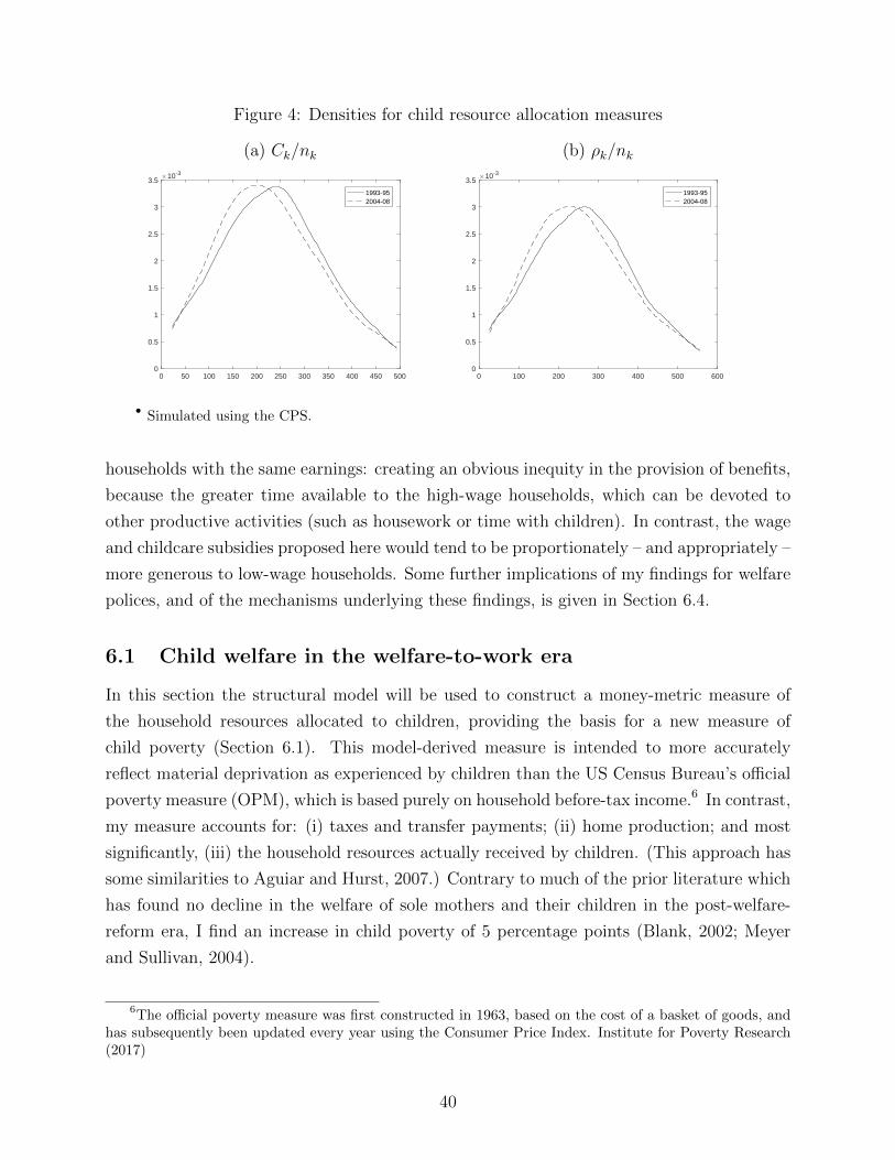
Figure 4: Densities for child resource allocation measures

(a) Ck/nk (b) ρk/nk

0 50 100 150 200 250 300 350 400 450 5000

0.5

1

1.5

2

2.5

3

3.5#10-3

1993-952004-08

0 100 200 300 400 500 6000

0.5

1

1.5

2

2.5

3

3.5#10-3

1993-952004-08

• Simulated using the CPS.

households with the same earnings: creating an obvious inequity in the provision of benefits,

because the greater time available to the high-wage households, which can be devoted to

other productive activities (such as housework or time with children). In contrast, the wage

and childcare subsidies proposed here would tend to be proportionately – and appropriately –

more generous to low-wage households. Some further implications of my findings for welfare

polices, and of the mechanisms underlying these findings, is given in Section 6.4.

6.1 Child welfare in the welfare-to-work era

In this section the structural model will be used to construct a money-metric measure of

the household resources allocated to children, providing the basis for a new measure of

child poverty (Section 6.1). This model-derived measure is intended to more accurately

reflect material deprivation as experienced by children than the US Census Bureau’s official

poverty measure (OPM), which is based purely on household before-tax income.6 In contrast,

my measure accounts for: (i) taxes and transfer payments; (ii) home production; and most

significantly, (iii) the household resources actually received by children. (This approach has

some similarities to Aguiar and Hurst, 2007.) Contrary to much of the prior literature which

has found no decline in the welfare of sole mothers and their children in the post-welfare-

reform era, I find an increase in child poverty of 5 percentage points (Blank, 2002; Meyer

and Sullivan, 2004).

6The official poverty measure was first constructed in 1963, based on the cost of a basket of goods, andhas subsequently been updated every year using the Consumer Price Index. Institute for Poverty Research(2017)

40

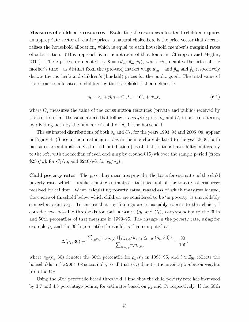
Measures of children’s resources Evaluating the resources allocated to children requires

an appropriate vector of relative prices: a natural choice here is the price vector that decent-

ralises the household allocation, which is equal to each household member’s marginal rates

of substitution. (This approach is an adaptation of that found in Chiappori and Meghir,

2014). These prices are denoted by p = (wm, pm, pk), where wm denotes the price of the

mother’s time – as distinct from the (pre-tax) market wage wm – and pm and pk respectively

denote the mother’s and children’s (Lindahl) prices for the public good. The total value of

the resources allocated to children by the household is then defined as

ρk = ck + pkq + wmtm = Ck + wmtm (6.1)

where Ck measures the value of the consumption resources (private and public) received by

the children. For the calculations that follow, I always express ρk and Ck in per child terms,

by dividing both by the number of children nk in the household.

The estimated distributions of both ρk and Ck, for the years 1993–95 and 2005–08, appear

in Figure 4. (Since all nominal magnitudes in the model are deflated to the year 2000, both

measures are automatically adjusted for inflation.) Both distributions have shifted noticeably

to the left, with the median of each declining by around $15/wk over the sample period (from

$236/wk for Ck/nk and $246/wk for ρk/nk).

Child poverty rates The preceding measures provides the basis for estimates of the child

poverty rate, which – unlike existing estimates – take account of the totality of resources

received by children. When calculating poverty rates, regardless of which measures is used,

the choice of threshold below which children are considered to be ‘in poverty’ is unavoidably

somewhat arbitrary. To ensure that my findings are reasonably robust to this choice, I

consider two possible thresholds for each measure (ρk and Ck), corresponding to the 30th

and 50th percentiles of that measure in 1993–95. The change in the poverty rate, using for

example ρk and the 30th percentile threshold, is then computed as:

∆(ρk, 30) =

∑i∈I08 πink,(i)1ρk,(i)/nk,(i) ≤ τ93(ρk, 30)∑

i∈I08 πink,(i)− 30

100.

where τ93(ρk, 30) denotes the 30th percentile for ρk/nk in 1993–95, and i ∈ I08 collects the

households in the 2004–08 subsample; recall that πi denotes the inverse population weights

from the CE.

Using the 30th percentile-based threshold, I find that the child poverty rate has increased

by 3.7 and 4.5 percentage points, for estimates based on ρk and Ck respectively. If the 50th

41

percentile is used, these figures rise slightly to 4.5 and 5.2. I thus conclude that for the

children of sole mothers (without a college degree), the child poverty rate rose by around

four percentage points in the decade following the introduction of TANF. My results stand

in contrast to calculations based on the OPM, which suggest that the child poverty rate has

decreased by 6.5 percentage points to 43.9 per cent, among the children of sole mothers,

over the same period (Child Trends Databank, 2017). They also differ from the findings of a

number of authors who have attempted to address some of these shortcomings of the OPM,

but have nevertheless found little evidence for an increase in child poverty rates since 1996

(Blank, 2002; Meyer and Sullivan, 2004).

The principal reason for these differences is that these authors still rely on household-level

income or consumption to measure material well-being, whereas I take account of the how

those resources are allocated within the household. Since 1996 the decline in the generosity of

cash welfare has been effectively compensated for by an increase in time spent in paid work,

and thus in before-tax incomes (recall Figure 2 above, and the accompanying discussion).

This has come largely at the expense of time spent in housework, which has fallen at the

median by just over 1 hr/wk between 1996 and 2008. Together with a decline in spending

public consumption – the median of which fell by $17/wk to $259/wk in 2005–08 – this has

resulted in a significant reduction in the output of the home-produced public good. It is this

reduction that is largely responsible for the increase in child poverty, as I have measured

it, something which measures based on household-level income or consumption will fail to

capture.

The preceding calculations – similarly to those of Blank (2002) and Meyer and Sullivan

(2004) – fail to account for any demographic shifts that might have occurred over the period,

such as changes to the average educational attainment or fertility of sole mothers. To remedy

this, I take the entire sample of sole-mother households from the CPS for 1993–2008, treating

them as though they were drawn from 1993 (so applying the 1993 tax-and-welfare system,

and imputing their wages using the 1993–95 estimates of the wage equation, etc.), and

computing the poverty thresholds on this basis. I then counterfactually apply the 2008

tax and welfare system to these households; re-solving the households’ problems yields an

estimate of ∆(ρk, 30) in which all demographic factors are held constant. The estimated

change in child poverty rates is 1.4 and 1.6 for ρk and Ck respectively using the 30th percentile

threshold, and 2.8 and 3.4 for the 50th percentile threshold. Demographic shifts would thus

seem to account for only about 2 percentage points of the change in the poverty rate over this

period, and so are insufficient to overturn the conclusion that TANF has had a deleterious

effect on child poverty.

42

Table 6: Effect of AFDC/TANF on household choices and welfare

Mean responses for the subgroup affected by the policy change

∆hm ∆tm ∆qm ∆qNetcost∗

CVkPassthru.∗

Grp.size∗

1 2 3 4 5 6 7 8

Policy counterfactuals

1 AFDC replaces TANF† -13.3 0.7 1.4 1.4 106.9 13.6 12.7 23.3

EITC expansion‡ 0.2 0.0 1.0 1.0 19.6 6.7 34.2 31.7

Introduction of policy, for years indicated §

3 TANF (1996–2008) -11.7 0.6 1.6 1.9 102.3 17.3 16.9 8.3

AFDC (1993–95) -19.7 1.2 2.8 4.3 183.3 35.4 19.3 25.9

EITC (1996–2008) 1.1 0.3 0.3 2.6 50.3 20.4 40.6 65.8

• Reports the results of counterfactual exercises conducted using the model, as described in Section 6.2. Units:net cost and CVk are in $/wk (2000 dollars); hm, qm and tm in hr/wk; pass thru. and grp. size in percentagepoints.

∗ Net cost is the cost of the policy intervention to the government, calculated as the increase in net transfers(benefits paid less taxes received) paid to households as a result of the policy. Pass thru. is CVk divided bythe net cost (in percentage points; see (6.3)). Grp. size is the percentage of households (sole mothers withouta college degree) affected by the policy change.

† Baseline is the tax and welfare system in place over 1996–2008; in the counterfactual, AFDC as it existed in1995 is introduced in each of these years (suitably adjusting programme benefits for inflation).

‡ Baseline is the tax and welfare system in place over 1996–2008; in the counterfactual, I introduce additionalbenefit payments for one-child families, as proposed by Hoynes (2014).

§ In each case, the baseline is the tax and welfare system in place over the specified period, sans the indicatedpolicy; this policy is (re-)introduced in the counterfactual.

6.2 PROWRA, child welfare and maternal labour supply

While it is clear that child welfare has declined since 1996 – even when changes in the

composition of the sample of sole mothers are controlled for – the extent to which this is a

direct result of the PROWRA reforms requires further analysis. I therefore use the model

to perform counterfactual experiments that allow me to identify the consequences of the

introduction of TANF, and also of the expansion of the EITC that occurred during the

same epoch. As well as determining how the allocation of household resources has altered

as a result of these policies, these exercises allow me to make a more reliable estimate of

their welfare effects. (Whereas the comparisons of ρk and Ck made above involve the use

of a different set of relative prices across the two comparison periods, below I am able to

43

construct a compensating variation-type measure that abstracts from such price changes.)

Results are displayed in Table 6. (This summarises the main results; a more complete

record is given by Table 13 in Appendix E.) The first counterfactual experiment (row 1)

reverses the PRWORA reforms: the baseline is the actual tax and welfare regime over

1996–2008, from which TANF is counterfactually replaced by AFDC (as it was in 1995,

adjusting for inflation). Columns 1–4 report the change in mother’s time use and in the

production of the public good, by subtracting the outcome in the baseline (TANF) from the

outcome under the counterfactual policy (AFDC), and averaging this over the subgroup of

households affected by the policy change (those which either receive TANF in the baseline, or

AFDC in the counterfactual). Columns 5–7 summarise the overall cost (to the government)

of the policy change, and quantify its effect on children’s welfare; column 8 reports the

proportion of households affected by the intervention. I shall now give a brief discussion of

the methodology used to compute the figures in columns 4–7, before discussing the results.

Measuring welfare effects and programme costs To quantify the welfare consequences

of PROWRA (and other counterfactual interventions) in money-metric terms, I use the fol-

lowing compensating variation-type measure. Let p0 denote the price vector that decent-

ralises the household’s allocation in the baseline; ρ0k the associated value of the children’s

allocation, computed as per (6.1) above; and K1

the children’s utility under the counterfac-

tual policy. I then compute

CVk = min∆ρ∈R

max

BC(p0,ρ

0k+∆ρ)

K(ck, tm, q) ≥ K1

, (6.2)

where BC(p, ρ) = (ck, tm, q) ∈ R+ | ck + wmtm + pkq ≤ ρ.7 CVk can thus be interpreted as

the amount the children would need to be paid in the baseline, to be as well-off as under the

counterfactual policy, if they were able to purchase consumption, time with their mother,

and the public good at the prices p0 with an ‘income’ of ρ0k + ∆ρ.8

7I also construct an analogous measure for the mother: but since my focus here is on children this isonly reported in the tables in Appendix E, where it is denoted as CVm. To compute this, I first determine

the utility U1

that the mother enjoys under the counterfactual policy (here, AFDC), and then calculate theadditional income (provided as a lump-sum transfer) that the household would need in the baseline (i.e.

under TANF) to achieve a utility of exactly U1. (Note that CVm will be negative for households that are

worse off under AFDC.)8Because the household’s objective is separable in children’s utility, a second interpretation of CVk is

also available (see Browning, Chiappori, and Weiss, 2011, Ch. 4). Suppose I were to provide the householdwith an additional lump-sum transfer ∆y, which it could allocate however it liked, but which was chosen

so as to be exactly sufficient to raise the children’s utility to K1. Then using p0 to evaluate the resultant

change in the child’s resources would yield ∆ck + w0m∆tm + p0k∆q = CVk .

44

The policy change considered in my first counterfactual exercise is far from being revenue

neutral, as AFDC is considerably more generous than TANF. The overall cost of the inter-

vention can be computed by subtracting net government tax revenues (counting transfers as

a diminution of those revenues) in the baseline from those in the counterfactual; I term this

the net cost, and report its average in column 5. This measure takes account of households’

behavioural responses to the policy change, and so in this case may differ markedly from a

simple comparison of the benefits paid out under AFDC with those paid out under TANF.

(Insofar as the introduction of AFDC tends to reduce labour supply, the ‘net cost’ as com-

puted here will tend to be higher than might be suggested by such a naive calculation.) To

facilitate the comparison of AFDC and TANF with other policies, in terms of their relative

efficacy at improving child welfare, I define the pass-through rate of a policy as

pass-through rate =CVk

net cost, (6.3)

(expressed as a percentage). This can be interpreted as the proportion of the welfare spending

that gets through to children.

Replacing TANF with AFDC; and some other counterfactuals The results suggest

that the 23 per cent of sole mothers (without a college degree) who are affected by the policy

change would work (on average) 13 fewer hours per week. Most of this newly freed time

would be enjoyed as additional leisure, but they also spend just over half an hour more with

children, and an hour and a half extra per week in housework (cols 1–3). Qualitatively, this

mirrors the increase in market work and reduced time spent in housework over 1996–2008,

but only explains a part of those changes.

Reintroducing AFDC is estimated to improve the welfare of the affected children by

almost $8/wk, in terms of CVk (col 6). Recall from the previous section that, in terms of

ρk/nk, the median child was $17/wk worse off in 2004–08 relative to 1993–95. Given that

the second figure controls for neither demographic shifts in the sample of sole mothers, nor

changes in the relative (decentralising) prices of household resources, whereas the former

does, the two figures seem broadly comparable. (Note that there are on average only 1.3

children per family in my sample, so that the fact that CVk is not expressed in per-child

terms matters relatively little here.)

In view of this, it might be argued that reintroducing AFDC would go a considerable way

to remedying the decline in children’s welfare that has occurred since 1996. However, such a

conclusion must be weighed against the cost of such a policy change, which is estimated to be

on the order of almost $100/wk (col 5). This implies a pass-through rate of 8 per cent (col 7).

45

To give some context for this figure, I conduct two further counterfactual exercises. In the

first, the the baseline is the existing tax and welfare policies without TANF (for 1996–2008),

which is then (re-)introduced in the counterfactual. This is reported in row 3 of the table;

row 4 reports the outcome of an analogous exercise, performed with respect to AFDC (and

for the years 1993–1995). The pass-through rates associated with both programmes are

between 15 and 20 per cent.

In fact, relative to the EITC, neither AFDC nor TANF is particularly effective at tar-

geting resources to children. Repeating the same exercise for the EITC yields an estimated

pass-through rate of almost 41 per cent, more than twice that of AFDC or TANF (row 5,

col 7). The results also indicate the EITC is in fact far more effective at increasing maternal

labour supply than TANF, despite the latter being regarded as the archetypal ‘welfare to

work’ programme. Because only a third of TANF enrollees meet the work requirements, for

most it has more the character of a lump-sum transfer – albeit one that may involve some

disutility to the recipient – and so has the expected income effect of reducing labour supply.

The EITC, on the other hand, by reducing the returns to work for households with a broad

range of incomes, has a positive (albeit small) effect on maternal labour supply.9

6.3 Alternatives to welfare-to-work programmes

In light of the preceding results, the EITC appears to be considerably more effective than

either AFDC to TANF in terms of promoting maternal labour supply and targeting house-

hold resources to children (per dollar spent). This finding motivates the search for altern-

atives to TANF, which might better fulfil these two objectives. Below I examine several

policies that encourage labour supply by increasing the net returns to working, rather than

by sanctioning enrollees who fail to meet mandated work requirements: these take the form

of childcare subsidies and wage subsidies.

Since eligibility for the EITC depends only on total earnings, the EITC does not dis-

criminate between households in which the mother: (a) earns a low wage and works full

time; and (b) earns twice that wage, and only works part time. From the perspective of

the model developed in this paper, there are other valuable activities to which a mother’s

time might be devoted – in particular, housework and time with her children. Once these

9Hoynes (2014) has recently suggested that the EITC benefits be increased for one-child families: thiswould be particularly beneficial for sole mothers, 66 per cent of whom only have one child. I evaluate thisproposal by counterfactually expanding the EITC from the baseline of the actual tax and welfare systemin place in 1996–2008, in the manner proposed by Hoynes (2014; see that paper for the exact details of herproposal). Her proposed changes would indeed be effective at targeting household resources to the childrenof sole mothers: the estimated pass-through rate is 32 per cent, and the policy reaches roughly 50 per centof one-child households (see row 2, col 7–8).

46

are accounted for, household (b) would seem to be much better off than household (a): thus

it must be counted a shortcoming of the EITC that it would pay exactly the same subsidy

to both. In effect, the EITC ignores the value of time spent in activities outside of market

work. One way of resolving this is to provide a subsidy that is proportionately more generous

to lower-wage – as distinct from lower-earnings – households. Hence I am led to consider

policies that increase the net return to an hour’s work: for example, the $1/hr wage subsidy

proposed below would pay twice as much to household (a) as to household (b).

Childcare subsidies For sole mothers with no access to sources of free informal childcare

(such as might be provided by relatives), the pre-tax net return to an hour’s work is the

wage, less the cost of an additional hour’s worth of childcare. On average, sole mothers

who work more than 20 hr/wk spend $32/wk on childcare for each child ages under 5, and

$15 per week for each child aged 6 to 13 (in the SIPP). Childcare subsidies thus provide an

effective means of raising the net returns to work for this group. At present, means-tested

subsidies are available in the form of a tax credit, the CDCTC, which delivers a maximum

30 per cent rebate to eligible households.

I conduct three counterfactual experiments related to childcare subsidies. In the first,

the baseline is the actual tax and welfare system in 1996–2008, without the CDCTC, which

is then (re-)introduced in the counterfactual. In the second and third, the baseline includes

the CDCTC, which is then alternately replaced by universal free childcare, or expanded

along the lines proposed by Ziliak (2014), who has suggested that CDCTC should provide

more generous rebates to low-income households (see that paper for the specific details of

his proposal). A summary of the main results appear in the first two rows of Table 7 (a

complete listing appears in Table 14 in Appendix E).

Most striking are the high pass-through rates for children: almost 100 per cent for CD-

CTC, 50 per cent for free childcare, and 40 per cent for the Ziliak (2014) expansion (see

rows 1-2, col 7). The last two are twice the pass-through rate for TANF, and comparable

to that of the EITC. Children benefit because the household’s income increases – not only

directly, because childcare is cheaper, but also indirectly, via an increase in maternal labour

supply (rows 1–2, col 1 in Table 7). This additional income is directed both to their private

consumption, and to public consumption. Although children do receive less maternal time

as a result of CDCTC, the magnitude of this decline is only 25 per cent of the increase in

maternal labour supply. All three policies are also considerably more effective than either

TANF or the EITC at promoting maternal labour supply.

Previous work on the effect of childcare on child development has focussed on the qual-

ity of care provided at home relative to childcare centres (Dustmann and Schonberg, 2012;

47

Table 7: Alternatives to welfare-to-work programmes

Mean responses for the subgroup affected by the policy change

Net Pass Grp.∆hm ∆qm ∆tm ∆q cost∗ CVk thru.∗ size∗

1 2 3 4 5 6 7 8

Childcare policies†

1 CDCTC 3.1 -0.5 -0.8 1.2 14.8 14.8 99.7 11.3

Free childcare 15.2 -1.0 0.2 5.7 101.4 50.2 49.5 38.0

Expansion 6.2 0.2 0.0 5.7 51.7 19.8 38.3 31.0

TANF eliminated; replaced by indicated policy†

4 Free childcare 10.3 -0.9 -0.9 3.7 86.5 35.3 40.8 46.2

Flat wage subsidy 1.2 0.0 0.0 0.9 10.6 8.1 76.5 93.5

Targeted wage subsidy 5.0 0.5 0.3 4.8 67.9 33.6 49.5 64.1

• Reports results of counterfactual exercises described in Section 6.3. Only households in years 1996–2008 of thesample are exposed to the policies. Units: net cost and CVk are in $/wk (2000 dollars); hm, qm and tm inhr/wk; pass thru. and grp. size in percentage points.

∗ For definitions of net cost, pass thru., and grp. size, see the corresponding note to Table 6.† In CDCTC, the baseline is the tax and welfare system in place over 1996–2008, sans CDCTC, which is (re-

)introduced in the counterfactual. Expansion additionally expands the CDCTC in the manner proposed byZiliak (2014). In free childcare, the baseline additionally includes CDCTC, which in the counterfactual isreplaced by universal free childcare.

‡ In each exercise, the baseline is the tax and welfare system in place over 1996–2008; in the counterfactual,TANF is eliminated and replaced by the policy indicated.

48

Fiorini and Keane, 2014). Quality of care is certainly one channel through which child-

care subsidies may affect child outcomes, but my results highlight another channel, which

works through the effect that these subsidies have on the allocation of household resources.

These two channels may help account for the apparently contradictory findings of two re-

cent studies examining the introduction of universal childcare: Baker, Gruber, and Milligan

(2008) find substantially negative effects on child outcomes among middle- and high-income

two-parent families (in Canada), while Havnes and Mogstad (2014) find positive effects for

lower-income households (in Norway). For less educated (and likely low-income) sole moth-

ers, the additional income that the household receives may be highly beneficial for children

– as my results forcefully contend – whereas for highly educated (and likely high-income)

households, childcare quality might be more important.

Wage subsidies Wage subsidies directly raise the net returns to work. Rows 4–6 in

Table 7 summarise the results of three counterfactual exercises that replace TANF with a

wage subsidy. In each case, the baseline is the actual tax and welfare regime over 1996–2008,

and the counterfactual consists of eliminating TANF and introducing one of the following

policies: universal free childcare (row 4); a flat-rate wage subsidy of $1/hr (row 5); or a wage

subsidy targeted at low-wage earners, which brings all wages up to a minimum of $11.60/hr

(row 6; in 2000 dollars). ($11.60 in 2000 corresponds to $15 in 2018 dollars; this is motivated

by the $15/hr minimum wage that is planned for New York in 2018.)

Each of these policies raise household income directly by increasing the returns to work,

and indirectly by also promoting maternal labour supply. Free childcare increases labour

supply by 10 hr/wk on average, the flat-rate wage subsidy by a little over 1 hr/wk and the

targeted wage subsidy by 5 hr/wk (rows 4–6, col 1; note that these averages are computed for

the sub-populations affected by the respective policy changes, and express changes relative

to a baseline in which TANF is in place). Since these labour supply responses raise taxable

earnings, the net cost of all these programmes (measured by the net change in government

taxes and transfers) is much lower than the gross benefits paid to households (compare cols

8 and 9, rows 4–15, in Table 14 in Appendix E).

Wage subsidies also achieve high pass-through rates. For example, the $1/hr wage subsidy

raises child welfare (in terms of CVk) by $8/wk with a pass-through rate of 77 per cent (row 5,

cols 7–8 in Table 7). The targeted wage subsidy costs $34/wk per recipient, and has a pass-

through rate of 50 per cent (row 6, cols 7–8).

49

6.4 Implications for welfare policies

Overall, my results suggest that policies that increase the net returns to working, are more

effective than TANF both at encouraging maternal labour supply, and in targeting household

resources to children. TANF provides sole mothers with the option of either: (a) working

30 hr/wk and claiming benefits, if their incomes are still sufficiently low; or (b) claiming

benefits without meeting that work requirement, at the cost of having to engage in some

other time-consuming activity, such as a job training programme. Most TANF enrollees (66

per cent in 2008) do not meet the work requirements, and so for them TANF has more the

character of a lump-sum transfer, and thus tends to reduce their labour supply.

As to why TANF fails to meet one its principal objectives, my results suggest that the

30 hr/wk work requirement is set too high to induce enough sole mothers to increase their

labour supply to this level: although 9 per cent of my sample (both in the CE and CPS)

have wages low enough that they would be eligible for TANF if they worked 30 hr/wk, only

22 per cent of these households do so. (They would be entitled an average of $58/wk from

TANF, relative to earnings of $180/wk at the 25th percentile.) For the remainder of these

women, their wages are so low that for the most part their time is better spent in alternative

activities, even with the additional work subsidy offered by TANF (at 30 hr/wk); average

hours worked by the entire group being only 23hr/wk. For many women, having to work

30 hr/wk week would be too much of distortion of the optimal allocation of their time.

In view of this, it is perhaps not surprising that policies which increases the net returns

to work, by a small amount for everyone, are more effective at promoting maternal labour

supply than is TANF. Such policies are also much more beneficial for children, in the sense

of achieving higher pass-through rates. A key reason for this lies in their effect on home

production. Recall from Section 6.1 that we observed an increase in child poverty rates

after 1996, and that this was associated with a simultaneous decline in the production of

the public good. The policies considered in Section 6.3 would be able to help reverse this

decline, by stimulating home production at a much lower cost than can either TANF (or

AFDC, for that matter). For example, when TANF is replaced with free childcare or the

targeted wage subsidy, it increases the output of the public good at an effective cost of under

$15/wk, whereas when TANF is replaced with AFDC, although public good production also

rises, the additional units of the public good cost almost $200/wk (these figures are arrived

at by dividing the increment in the output of the public good by the net cost of the policy

change).

50

7 Conclusion

The introduction of TANF was the most significant change to the US welfare system in the

postwar era. TANF was intended to reduce welfare dependency and promote labour supply,

through work requirements and lifetime limits. But while caseloads have indeed fallen, and

hours worked have increased, my results indicate that these apparent successes have come

at the expense of children’s welfare.

Using a structural model of household decision-making and resource allocation, I find that

the welfare of the children of sole mothers has been materially worsened by the introduction

of TANF. Because of the prohibitively high work requirements (30 hr/wk), low-wage women

typically do not find it worthwhile to work sufficiently many hours to be eligible for TANF,

even though their weekly earnings put them well below the poverty line. For this group, the

main consequence of PRWORA was simply a withdrawal of the benefits they had previously

been entitled to (under AFDC). This loss of income has been partly offset by an increase

in their labour supply, but the net result of this has been detrimental to children, because

it has left mothers with less time to devote to home production. Using the model to value

the household resources allocated to children, and thus account for the effects of the tax and

welfare system, the intra-household allocation of resources, and home production, I find that

child poverty rates have risen by four percentage points since the introduction of TANF,

among the children of sole mothers (without a college degree).

To the extent that work requirements are not rigidly enforced – currently, two-thirds of

TANF recipients fail to meet these requirements – TANF continues to provide something

like a traditional safety net for low-income households. However, states are now coming

under increasing pressure to ensure that a higher proportion of enrollees meet the work

requirements: if they were to do so, then even this already very diminished safety net would

disappear, with further negative consequences for low-income households.

I consider a number of alternatives to welfare-to-work programmes, which encourage

labour supply by instead increasing the return from working, rather than by sanctioning non-

compliers: these are free childcare, and two types of wage subsidy. Each of these alternatives

is more effective at promoting labour supply than is TANF, and raises household income by

increasing not only the returns from working, but also hours worked. These policies are also

far more successful at targeting household resources to children, with all having estimated

pass-though rates in excess of 40 per cent (as compared with 17 per cent for TANF).

New York City, California, Chicago, Seattle, and Washington D.C. all plan to raise

minimum wages to $15/hr during the next decade. (The targeted wage subsidy of $11.60 in

2000 dollars, considered above, is equivalent to a $15 wage subsidy in 2016.) If these higher

51

minimum wages do not significantly attenuate the demand for low-skilled labour, nor raise

prices so far as to absorb the real gains from the wage increase (for this group), my results

suggest that children in sole-parent households might be the unexpected beneficiaries of such

a policy, as much of the additional income will translate into tangible resources for these

children.

8 References

Aguiar, M., and E. Hurst (2007): “Life-cycle prices and production,” American EconomicReview, 97(5), 1533–1559.

Apps, P., and R. Rees (1996): “Labour Supply, Household Production and Intra-family WelfareDistribution,” Journal of Public Economics.

Baker, M., J. Gruber, and K. Milligan (2008): “Universal Child Care, Maternal LaborSupply, and Family Well-Being,” Journal of Political Economy, 116(4), 709–745.

Blank, R. M. (2002): “Evaluating welfare reform in the United States,” Journal of EconomicLiterature, 40(4), 1105–1166.

Blundell, R., M. Costa Dias, C. Meghir, and J. Shaw (2016): “Female labor supply, humancapital, and welfare reform,” Econometrica, 84(5), 1705–1753.

Blundell, R., and A. Shephard (2011): “Employment, Hours of Work and the Optimal Taxa-tion of Low-Income Families,” Review of Economic Studies.

Blundell, R., and I. Walker (1986): “A Life-cycle Consistent Empirical Model of FamilyLabour Supply Using Cross-Section Data,” Review of Economic Studies.

Brooks-Gunn, J., and L. Markman (2005): “The contribution of parenting to ethnic and racialgaps in school readiness,” The Future of Children, 15(1), 139–168.

Browning, M., P.-A. Chiappori, and Y. Weiss (2011): Familiy Economics. Online Book.

Chang, Y., and F. Schorfheide (2003): “Labor-supply shifts and economic fluctuations,”Journal of Monetary Economics, 50(8), 1751–1768.

Cherchye, L., B. De Rock, and F. Vermeulen (2012): “Married with children: A collect-ive labor supply model with detailed time use and intrahousehold expenditure information,”American Economic Review, 102(7), 3377–3405.

Chiappori, P.-A., and C. Meghir (2014): “Intra-household welfare,” Discussion paper, NationalBureau of Economic Research.

Child Trends Databank (2017): “Children in poverty,”https://www.childtrends.org/indicators=children-in-poverty, Accessed: 2017-08-10.

52

Crouse, G., and S. Macartney (2016): “Welfare Indicators and Risk Factors,” Discussionpaper, U.S. Department of Health and Human Services.

Dahl, G., and L. Lochner (2011): “The impact of family income on child achievement: evidencefrom changes in the Earned Income Tax Credit,” American Economic Review.

Del Boca, D., C. Flinn, and M. Wiswall (2014): “Household Choices and Child Develop-ment,” Review of Economic Studies.

Dunbar, G., A. Lewbel, and K. Pendakur (2013): “Children’s Resources in Collective House-holds: Identification, Estimation and an Application to Child Poverty in Malawi,” AmericanEconomic Review.

Dustmann, C., and U. Schonberg (2012): “Expansions in maternity leave coverage and chil-dren’s long-term outcomes,” American Economic Journal: Applied Economics, 4(3), 190–224.

Fiorini, M., and M. Keane (2014): “How the Aloocation of Children’s Time Affects Cognitiveand Non-cognitive Development,” Journal of Labor Economics.

Gourieroux, C., A. Monfort, and E. Renault (1993): “Indirect inference,” Journal of Ap-plied Econometrics, 8(S1), S85–S118.

Grogger, J., and C. Michalopoulos (2003): “Welfare Dynamics under Time Limits,” Journalof Political Economy, 111(3).

Havnes, T., and M. Mogstad (2014): “Is universal child care leveling the playing field?,” Journalof Public Economics.

Hoynes, H. (1996): “Welfare Transfers in Two Parent Families: Labor Supply and Welfare Par-ticipation under AFDC-UP,” Econometrica.

(2014): “Proposal 11: Building on the Success of the Earned Income Tax Credit,” inImproving Safety Net and Work Support. The Hamilton Project.

Institute for Poverty Research (2017): “How is poverty measured in the Unite States,”http://www.irp.wisc.edu/faqs/faq2.htm, Accessed: 2017-08-10.

Isaacs, J., K. Toran, H. Hahn, K. Fortuny, and C. Steuerle (2012): “Kids’ share 2012:report on federal expenditures on children through 2011,” Discussion paper, The Urban Institute.

Kimmel, J., and R. Connelly (2007): “Mothers’ Time Choices: Caregiving, Leisure, HomeProduction, and Paid Work,” The Journal of Human Resources.

Lise, J., and S. Seitz (2011): “Consumption inequality and intra-household allocations,” TheReview of Economic Studies, 78(1), 328–355.

McGrattan, E. R., R. Rogerson, and R. Wright (1997): “An equilibrium model of thebusiness cycle with household production and fiscal policy,” International Economic Review, pp.267–290.

Meyer, B. D., and J. X. Sullivan (2004): “The effects of welfare and tax reform: the materialwell-being of single mothers in the 1980s and 1990s,” Journal of Public Economics, 88(7), 1387–1420.

53

(2008): “Changes in the consumption, income, and well-being of single mother headedfamilies,” American Economic Review, 98(5), 2221–2241.

Phillips, M. (2011): Whither opportunity? Rising Inequality, Schools, and Children’s LifeChanceschap. Parenting, time use, and disparities in academic outcomes, pp. 207–228. RussellSage Foundation.

Scarborough, H. S., and W. Dobrich (1994): “On the efficacy of reading to preschoolers,”Developmental Review, 14(3), 245–302.

Schott, L., L. Pavetti, and I. Finch (2012): “How states have spent federal and state fundsunder the TANF block grant,” Discussion paper, Center of Budget and Policy Priorities.

Snow, C. E., and D. E. Beals (2006): “Mealtime talk that supports literacy development,”New Directions for Child and Adolescent Development, 2006(111), 51–66.

Tamis-LeMonda, C. S., M. H. Bornstein, and L. Baumwell (2001): “Maternal responsive-ness and children’s achievement of language milestones,” Child development, 72(3), 748–767.

Ziliak, J. (2014): “Proposal 10: Supporting Low-Income Workers through Refundable Child-CareCredits,” in Improving Safety Net and Work Support. The Hamilton Project.

54

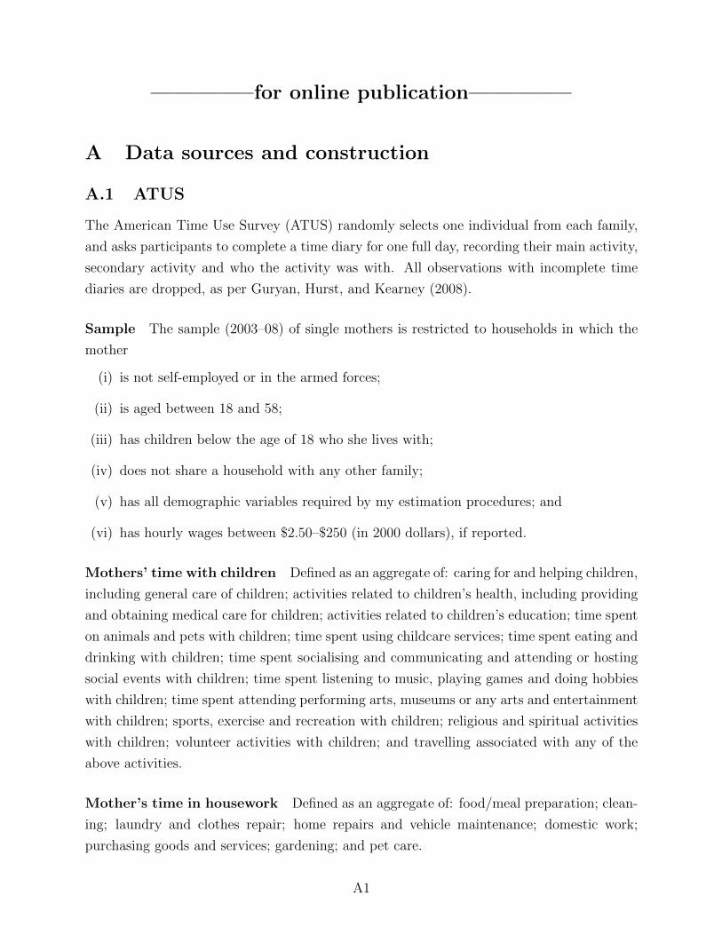
————–for online publication————–

A Data sources and construction

A.1 ATUS

The American Time Use Survey (ATUS) randomly selects one individual from each family,

and asks participants to complete a time diary for one full day, recording their main activity,

secondary activity and who the activity was with. All observations with incomplete time

diaries are dropped, as per Guryan, Hurst, and Kearney (2008).

Sample The sample (2003–08) of single mothers is restricted to households in which the

mother

(i) is not self-employed or in the armed forces;

(ii) is aged between 18 and 58;

(iii) has children below the age of 18 who she lives with;

(iv) does not share a household with any other family;

(v) has all demographic variables required by my estimation procedures; and

(vi) has hourly wages between $2.50–$250 (in 2000 dollars), if reported.

Mothers’ time with children Defined as an aggregate of: caring for and helping children,

including general care of children; activities related to children’s health, including providing

and obtaining medical care for children; activities related to children’s education; time spent

on animals and pets with children; time spent using childcare services; time spent eating and

drinking with children; time spent socialising and communicating and attending or hosting

social events with children; time spent listening to music, playing games and doing hobbies

with children; time spent attending performing arts, museums or any arts and entertainment

with children; sports, exercise and recreation with children; religious and spiritual activities

with children; volunteer activities with children; and travelling associated with any of the

above activities.

Mother’s time in housework Defined as an aggregate of: food/meal preparation; clean-

ing; laundry and clothes repair; home repairs and vehicle maintenance; domestic work;

purchasing goods and services; gardening; and pet care.

A1

Variance estimates for time-use measures For time with children and housework,

daily time diaries provide a consistent estimate of the average weekly time spent in these

activities, but yield an upwardly biased estimate of the weekly variance (Bruins and Duffy,

2015). Using a unique Dutch dataset (Tijdsbestedingsonderzoek, 2005), which provides a

complete set of daily time diaries for each respondent (i.e. one for every day of the week),

I estimate these variance measures to be upwardly biased by a factor of 1.5. The sample

variance moments for time with children and housework are therefore computed by multiply-

ing the (daily) sample variance computed from the ATUS time diaries by a factor of 0.67

(equivalently, the sample standard deviation is scaled down by a factor of 0.82).

A.2 AHTUS

Data on time spent in housework in 1995 is based on time diaries provided by the American

Heritage Time Use Study (AHTUS). Bad or incomplete diaries, as indicated in the AHTUS

documentation, were dropped; the sample is otherwise constructed exactly as for the ATUS.

Time spent in housework is aggregated from the same set of activities as for the ATUS.

A.3 CE

In constructing the Consumer Expenditure Survey (CE) sample I follow Blundell, Pistaferri,

and Preston (2008). The sample (1993–2008) is constructed identically to that of the ATUS

except that, owing to the problems discussed in Blundell, Pistaferri, and Preston (2008), the

age range in (ii) is modified to 25–58.

Public consumption expenditure This is defined to include food expenditures, property

taxes, mortgage interest, rent, household operations, utilities, fuel, and public services.

Non-labour income less savings Recall from the household budget constraint (3.7) that

‘non-labour income less savings’, y−s, is the difference between household non-durables con-

sumption and after-tax earnings. Non-durables expenditure is defined as total consumption

expenditure less expenditures on: house furnishings and equipment; outlays for other lodging;

mortgage principal outlays; maintenance, repairs and insurance; educational expenditures;

and personal insurance and pensions.

A.4 CPS

The CPS data is taken from the ‘CPS Merged Outgoing Rotation Groups’ provided by the

NBER website. The sample is restricted analogously to the ATUS.

A2

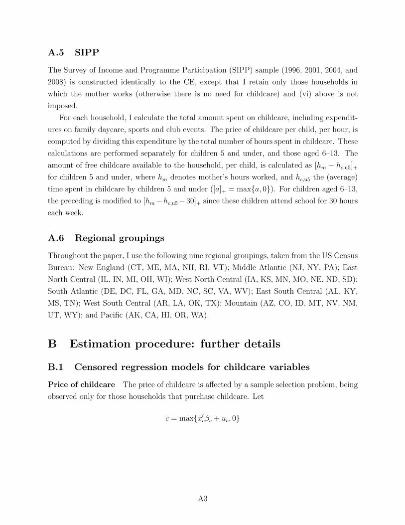
A.5 SIPP

The Survey of Income and Programme Participation (SIPP) sample (1996, 2001, 2004, and

2008) is constructed identically to the CE, except that I retain only those households in

which the mother works (otherwise there is no need for childcare) and (vi) above is not

imposed.

For each household, I calculate the total amount spent on childcare, including expendit-

ures on family daycare, sports and club events. The price of childcare per child, per hour, is

computed by dividing this expenditure by the total number of hours spent in childcare. These

calculations are performed separately for children 5 and under, and those aged 6–13. The

amount of free childcare available to the household, per child, is calculated as [hm − hc,u5]+

for children 5 and under, where hm denotes mother’s hours worked, and hc,u5 the (average)

time spent in childcare by children 5 and under ([a]+ = maxa, 0). For children aged 6–13,

the preceding is modified to [hm−hc,u5−30]+ since these children attend school for 30 hours

each week.

A.6 Regional groupings

Throughout the paper, I use the following nine regional groupings, taken from the US Census

Bureau: New England (CT, ME, MA, NH, RI, VT); Middle Atlantic (NJ, NY, PA); East

North Central (IL, IN, MI, OH, WI); West North Central (IA, KS, MN, MO, NE, ND, SD);

South Atlantic (DE, DC, FL, GA, MD, NC, SC, VA, WV); East South Central (AL, KY,

MS, TN); West South Central (AR, LA, OK, TX); Mountain (AZ, CO, ID, MT, NV, NM,

UT, WY); and Pacific (AK, CA, HI, OR, WA).

B Estimation procedure: further details

B.1 Censored regression models for childcare variables

Price of childcare The price of childcare is affected by a sample selection problem, being

observed only for those households that purchase childcare. Let

c = maxx′cβc + uc, 0

A3

denote the hours of childcare purchased for children aged 0–5. Assuming that (uc, up) are

jointly Gaussian, I may write

p− pmin = maxx′pβp + up, 0 = maxx′pβp + ρcuc + σpεp, 0

for the price of childcare for children aged 0–5, where εp ⊥⊥ uc and xc = (x′p, z′c)′. xp consists

of a constant, the age of the mother, two race dummies (white and black), a dummy for

tertiary education, and (nine) region dummies. zc consists of a Hispanic dummy and the age

of the youngest child.

I adopt the following control function approach to estimating βp:

(i) Tobit regression of c on xc: yields residuals uc.

(ii) Tobit regression of p− pmin on (xp, uc), using the subsample c > 0.

To produce separate estimates of βp for children aged 6–13, I run the above procedure a

second time, with (c, p) now recording the hours purchased and price of childcare for children

aged 6–13.

Hours of free childcare Estimation of the parameters in (4.7) is complicated by sample

selection and two-sided censoring. Suppose mother’s hours worked, hm, is generated accord-

ing to:

hm = maxx′hβh + uh, 0.

Assuming that (uh, ua) are jointly Gaussian, I may write

a = maxx′aβa + ua, 0 = maxx′aβa + ρhuh + σaεa, 0,

for the hours of free childcare available for children aged 0–5, where εa ⊥⊥ uh and xh =

(x′a, z′h)′. xa consists of the same variables as xp above, and additionally records whether the

family owns their residence. zh consists of a Hispanic dummy and the age of the youngest

child.

Now note that:

(i) a is observed only if hm > 0; and

(ii) even if hm > 0, the observed values of a are censored to lie in the interval [0, hm];

i.e. I observe a := mina, hm for these households. I therefore adopt the following control

function approach to estimating βa:

A4

(i) Tobit regression of hm on xh: yields residuals uh.

(ii) ‘Double tobit’ regression of a on (x, uh), with hm as the right censor point (and zero

as the left censor point), using the subsample hm > 0.

To estimate the parameters of (4.7) for children aged 6–13, exactly the same approach is

used, except that now a refers to the hours of free childcare available for children aged 6–13,

and is observed only if hm − 30 > 0 (since these children spend 30 hr/wk in school).

B.2 Household members’ private consumption

Although the CE records the total private consumption of the household, it does not provide

a breakdown of that consumption across family members. However, it does provide data on

some private assignable goods, in particular clothing, which has been used in prior literature

to estimate household members’ individual private consumption. Here I adapt the procedure

developed by Dunbar, Lewbel, and Pendakur (2013) to estimate the breakdown of private

consumption. This is in turn used to construct (unconditional) sample means for mother’s

and children’s consumption, which are matched in estimation (as discussed in Section 4.4).

Suppose that there are N consumption goods: let cij denote expenditure on the jth

consumption good for person i ∈ m, k, and ci =∑

j∈J cij his (or her) total private con-

sumption expenditure. Under certain conditions on individual preferences, given by Dunbar,

Lewbel, and Pendakur (2013, Sec. II), the optimal choice of cij will be related to ci via

cijci

= (β0i + β1i log ci) . (B.1)

Dunbar, Lewbel, and Pendakur (2013) further show that if preferences are ‘similar across

types’, in the sense that β1m = β1k, then

cijC

= ηicijci

(B.2)

for i ∈ m, k, where C = cm + ck total private consumption expenditure.

With the aid of (B.1) and (B.2), it is possible to recover ci from observations on C and

(cm1, ck1) alone, i.e. from data on total household private consumption expenditure and on

a single assignable good – in my case, clothing. This involves first estimating the slope

coefficients in the regression

ci1C

= αi + (βηi) logC = αi + γi logC,

A5

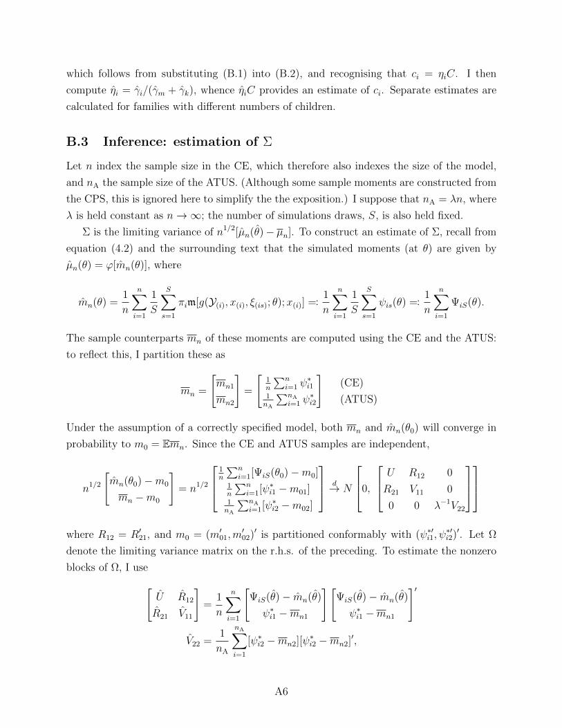
which follows from substituting (B.1) into (B.2), and recognising that ci = ηiC. I then

compute ηi = γi/(γm + γk), whence ηiC provides an estimate of ci. Separate estimates are

calculated for families with different numbers of children.

B.3 Inference: estimation of Σ

Let n index the sample size in the CE, which therefore also indexes the size of the model,

and nA the sample size of the ATUS. (Although some sample moments are constructed from

the CPS, this is ignored here to simplify the the exposition.) I suppose that nA = λn, where

λ is held constant as n→∞; the number of simulations draws, S, is also held fixed.

Σ is the limiting variance of n1/2[µn(θ)− µn]. To construct an estimate of Σ, recall from

equation (4.2) and the surrounding text that the simulated moments (at θ) are given by

µn(θ) = ϕ[mn(θ)], where

mn(θ) =1

n

n∑i=1

1

S

S∑s=1

πim[g(Y(i), x(i), ξ(is); θ);x(i)] =:1

n

n∑i=1

1

S

S∑s=1

ψis(θ) =:1

n

n∑i=1

ΨiS(θ).

The sample counterparts mn of these moments are computed using the CE and the ATUS:

to reflect this, I partition these as

mn =

[mn1

mn2

]=

[1n

∑ni=1 ψ

∗i1

1nA

∑nA

i=1 ψ∗i2

](CE)

(ATUS)

Under the assumption of a correctly specified model, both mn and mn(θ0) will converge in

probability to m0 = Emn. Since the CE and ATUS samples are independent,

n1/2

[mn(θ0)−m0

mn −m0

]= n1/2

1n

∑ni=1[ΨiS(θ0)−m0]

1n

∑ni=1[ψ∗i1 −m01]

1nA

∑nA

i=1[ψ∗i2 −m02]

d→ N

0,

U R12 0

R21 V11 0

0 0 λ−1V22

where R12 = R′21, and m0 = (m′01,m′02)′ is partitioned conformably with (ψ∗′i1, ψ

∗′i2)′. Let Ω

denote the limiting variance matrix on the r.h.s. of the preceding. To estimate the nonzero

blocks of Ω, I use[U R12

R21 V11

]=

1

n

n∑i=1

[ΨiS(θ)− mn(θ)

ψ∗i1 −mn1

][ΨiS(θ)− mn(θ)

ψ∗i1 −mn1

]′

V22 =1

nA

nA∑i=1

[ψ∗i2 −mn2][ψ∗i2 −mn2]′,

A6

which are assembled to construct Ω (note that λ is computed as nA/n). Finally, letting

Jϕ(m) = ∂mϕ(m) denote the Jacobian of ϕ with respect to m, I can estimate Σ using

Σ =[Jϕ(mn) −Jϕ(mn)

]Ω

[Jϕ(mn)′

−Jϕ(mn)′

].

C Parameter estimates

C.1 Models used for the imputation of missing variables

Table 8: Log wages, and non-labour income less saving

logwm (y − s)/100

1993–98 1999–03 2004–08 1993–98 1999–03 2004–08

Education

High school diploma 0.28 0.35 0.35 82.24 18.37 -17.64(0.09) (0.09) (0.11) (27.70) (31.95) (35.30)

Tertiary 0.46 0.58 0.58 75.33 -7.86 -0.43(0.10) (0.10) (0.12) (28.81) (31.08) (32.58)

Race

White 1.08 1.29 1.34 52.80 63.58 -21.29(0.15) (0.15) (0.18) (60.67) (68.50) (54.93)

Black -0.04 -0.11 0.05 22.30 41.16 -83.01(0.05) (0.05) (0.05) (61.92) (70.15) (56.82)

Mother’s age

Age 0.15 0.04 0.13 -5.08 5.85 -12.06(0.04) (0.02) (0.03) (13.00) (11.16) (10.69)

Age2/100 -0.18 -0.04 -0.15 2.83 -7.65 13.81(0.04) (0.03) (0.04) (16.67) (14.43) (13.94)

Case-Shiller house price index -20.21 -1265.90 287.96(6.26) (413.62) (137.32)

• Coefficient estimates for (4.5), obtained from the CE. Standard errors in parentheses. Units: wm in $/hr, y−s in $/wk(year 2000 dollars). All explanatory variables are interacted with dummy variables for the years 1993–98, 1999–2003,2004–08. Coefficients on region (nine) and year dummies are also estimated (suppressed from the table).

A7

Table 9: Price of childcare and availability of free childcare

Price Free care

pu5 po5 au5 ao5

Tertiary -0.80 2.29 -13.26 -11.66education (0.75) (1.03) (1.60) (1.37)

Mother’s age

Age 0.02 -0.4 6.75 5.76(0.23) (0.53) (0.45) (0.44)

Age2/100 -0.09 -0.07(0.01) (0.01)

Race

White 0.25 -0.40 49.29 35.64(0.56) (1.09) (2.51) (1.45)

Black 1.16 1.10 44.13 32.14(1.09) (1.67) (2.74) (1.75)

Regions∗

New England -0.20 0.16 -8.02 -5.70(0.87) (1.62) (1.69) (1.85)

Mid Atlantic -0.64 -0.67 0.78 1.00(1.00) (1.62) (1.46) (1.66)

East North Central -0.34 0.42 1.02 -6.65(0.78) (1.75) (2.16) (1.98)

West North Central -3.01 -0.71 7.37 5.16(1.29) (2.03) (1.47) (1.76)

South Atlantic -2.69 2.03 -7.17 -0.20(0.94) (1.92) (3.74) (2.17)

East South Central -1.44 1.79 2.08 4.52(1.09) (1.83) (2.03) (2.06)

West South Central -1.04 0.99 3.24 4.55(0.87) (1.80) (4.40) (1.67)

Mountain 0.11 0.07 -2.94 -7.14(0.03) (0.03) (1.54) (1.69)

• Coefficient estimates for (4.6) and (4.7), obtained from the SIPP. Standarderrors in parentheses. Units: pu5, po5 in $/hr; au5, ao5 in hr/wk.

∗ Regions taken from the US Census Bureau; omitted region is Pacific.

A8

C.2 TANF enrolment and lifetime limits

Table 10: Probit estimates for TANF receipt (sole mothers)

Demographic variables

Mother’s age 0.14 Has a child aged 0–2 0.23(0.00) (0.02)

Mother’s age2/100 -0.19 Has a child aged 0–5 0.32(0.00) (0.02)

White -0.18 Has a child aged 0–13 0.29(0.03) (0.02)

Black 0.28 Has more than one child -0.05(0.03) (0.01)

High school diploma -0.52(0.02)

Exposure to lifetime limits∗

z1 (‘never’) 0.28 z2 (‘partial’) 0.13(0.04) (0.02)

Years

1996–99 0.15 2003–05 0.21(0.03) (0.02)

2000–02 0.24(0.03)

Regions†

New England -0.38 South Atlantic -0.70(0.03) (0.04)

Mid Atlantic -0.55 East South Central -0.77(0.03) (0.03)

East North Central -0.35 West South Central -0.63(0.03) (0.03)

West North Central -0.72 Mountain -0.27(0.03) (0.03)

• Coefficient estimates for (4.9), obtained from the CPS (1996–2008, n = 25, 000). Standarderrors in parentheses.

∗ z1 = 1 if a mother’s youngest child was aged over 12 when time-limits were introducedin her state, so that she was never never subject to time limits. z2 = 1 if the mother’syoungest child was born before time limits were introduced, in which case she was onlypartially exposed to time limits.

† Regions taken from the US Census Bureau; omitted region is Pacific.

A9

C.3 Structural model

Table 11: Structural model parameter estimates

Mother’s utility

γm,c = exp(x′mβm,c + σm,cεm,c)

βm,c: constant -1.12 βm,c: some tertiary 0.73(0.95) education (0.50)

σm,c 0.10(0.95)

γm,l = exp(x′mβm,l + σm,lεm,l)

βm,l: constant -1.27 βm,l: some tertiary 1.78(0.89) education (0.61)

βm,l: wage equation 1.92 σm,l 0.27residual (0.95) (0.46)

ηm = 1 − exp(x′m,ηβm,η)

βm,η: constant -1.74 βm,η: some tertiary 0.69(0.38) education (0.24)

βm,η: youngest child 0.07aged 0–5 (0.38)

δk = exp(x′δkβδk + σδkεδk)

βδk : constant -0.84 βδk : youngest child 0.29(0.21) aged 0–5 (0.20)

βδk : more than one child 0.05 σδk 0.24(0.32) (0.16)

τ (utility cost of working) 0.14(0.02)

• Standard errors in parentheses, calculated as per Section 4.2. ε always denotes an i.i.d.standard Gaussian disturbance.

A10

Table 12: Structural model parameter estimates

Children’s utility

γk,c = exp(x′k,cβk,c + σk,cεk,c)

βk,c: youngest child 0.24 βk,c: youngest child -0.37aged 0–5 (0.45) aged 6–18 (0.29)

σk,c 0.44(0.17)

γk,t = exp(x′k,tβk,t + σk,tεk,t)

βk,t: youngest child -1.62 βk,t: youngest child -1.01aged 0–5 (0.36) aged 6–18 (0.15)

σk,t 0.45(0.10)

ηk = 1 − exp(x′k,ηβk,η)

ηk: constant -0.18 ηk: youngest child 1.43(0.41) aged 5 or under (1.54)

ηk: two or more 0.47children (0.26)

Home production

γq,c = exp(x′q,cβq,c + σq,cεq,c)

βq,c: youngest child 0.94 βq,c: youngest child 2.93aged 0–5 (0.16) aged 6–18 (1.00)

σq,c 0.55(0.14)

ηq = 1 − exp(x′q,ηβq,η)

βq,η: youngest child -0.50 βq,η: youngest child 0.62aged 0–5 (0.66) aged 6–18 (0.15)

• Standard errors in parentheses, calculated as per Section 4.2. ε always denotes an i.i.d.standard Gaussian disturbance.

A11

D Calculation of taxes and welfare payments

The calculation of household’s after-tax earnings is an important component of the model.

(Recall the discussion of the household’s budget constraint given in Section 3.2.) Details

of the relevant tax and benefit calculations, and the sources that are drawn upon to make

these calculations, are given below. In general, after-tax earnings will vary according to:

before-tax earnings; the number of children (aged 0–2, 0–5, 0–13, 0–16 and 0–18) in the

household; the age of youngest child; childcare expenditures; and the hours worked by the

mother.

D.1 Taxes

Federal taxes Federal tax parameters are taken from the Urban Institute’s Tax Policy

Centre (TPC) database. I first determine the tax-free threshold as the sum of the standard

deduction and the dependent exemption (multiplied by the number of dependants). Then

the usual bracketing formula is applied to income above this threshold.

State taxes State tax parameters, for those states that do have income taxes, are drawn

principally from the State Tax Handbook. These either take the form of a flat rate on before-

tax incomes (CT, IL, IN, NH, PA), or involve a similar bracketing calculation to that used

to compute federal taxes.

D.2 Tax credits

Parameters for the tax credits are drawn from the TPC. Each of these are means tested,

and are calculated on the following basis. As before-tax earnings y increases from zero, the

value of the credit increases linearly from zero, at rate rin. This is the phase-in region: once

a certain income level is reached, denoted yin, the credit stops increasing and remains at

b = rin · yin. Finally, beyond a certain threshold yout, the value of the credit declines linearly

with income to zero, at rate rout (the phase-out region). Mathematically, the value of the

credit for which a household is eligible can be expressed as:

credit(y) =

rin · y if y ≤ yin (phase-in)

b if y ∈ [yin, yout]

maxrout · [b− (y − yout)], 0 if y ≥ yout (phase-out)

(D.1)

A12

Figure 5: Federal tax credits

Weekly transfers and income (year 2000 dollars)

(a) EITC (b) CTC

0 100 200 300 400 500 600 700 800 900 10000

10

20

30

40

50

60

70

80

Income

Net

tran

sfer

1993

1996

2000

2004

2008

2012

0 500 1000 1500 2000 2500 30000

5

10

15

20

25

30

35

40

Income

Net

tran

sfer

1994

1996

2000

2004

2008

2012

• Calculated for a two-parent family with two children aged 0–16.

The household’s tax liabilities are then reduced by the magnitude of the credit. If the credit

is refundable, then the household receives any excess of the credit over its tax liabilities as

a payment.

Earned Income Tax Credit This credit is refundable. The formula for the federal EITC

is as in (D.1); the parameters (b, rin, rout, yin and yout) vary over time and with family size

(the number of children aged 0–16). The value of the credit for a [two-parent], two-child

family, is displayed in Figure 5. The state EITC is an additional credit that is calculated as

a proportion of the federal EITC benefit; this proportion varies across time and states (and

is zero in most states).

Child Tax Credit This credit is non-refundable. The formula for the credit is (D.1);

again its parameters vary over time and family size. The value of the credit is depicted in

Figure 5, which illustrates that the credit is not as strictly means tested as is the EITC.

Child and Dependent Care Tax Credit This credit is non-refundable. Its formula is

given by

A13

cdctc(y) =

minrin · c, cmax if y ≤ yin

min(rin − 0.01 · y−yin

2000/52

)· c, cmax

if y ∈ [yin, yout]

minrout · c, cmax if y ≥ yout

where c denotes the household’s childcare costs, and cmax the maximum value of the benefit.

D.3 Welfare payments

Supplemental Nutritional Assistance Program Parameters for SNAP are taken from

Eslami, Leftin, and Strayer (2012, Appendix G). Letting ynet = 0.8y−dstd, where dstd denotes

the standard deduction, the benefits (in the form of food stamps) for which a household is

eligible is given by:

snap =

b− 0.3 · ynet if y ≤ 0.3 · ypov and ynet ≤ ypov

0 otherwise

where b denotes the maximum benefit payable, and ypov the official poverty threshold.

Temporary Assistance for Needy Families Parameters for TANF are taken from the

Urban Institute’s Welfare Rules Database. The benefits for which are household is eligible

under TANF is calculated, for most states (excepting CT, HI, MO, NV, NJ, ND and WI),

from the positive part of

tanf = minb, r · [b− (y − d)] (D.2)

where b denotes the maximum benefit claimable, r is the rateable percentage, b the benefit

standard, y before-tax earnings, and d the disregard. Both the benefit standard and the

maximum benefit vary with the number of individuals in the family. In most states, TANF

can only be claimed for a maximum of five years, and the value of the disregard depends on

the number of years for which TANF has already been claimed. To simplify the calculations

– and because I do not observe the number of times that an individual has claimed TANF

– I set d to the average of these values. The disregard also depends on the amount that the

household spends on childcare, which I take account of in my calculations.

Aid to Families with Dependent Children AFDC is calculated using an identical

formula to (D.2); its parameters are drawn from the Urban Institute’s Trim3 database.

A14

E Policy counterfactuals: full listing of results

Table 13: Effect of AFDC/TANF on household choices and welfare

∆cm ∆ck ∆cq ∆hm ∆tm ∆qm ∆qNetcost∗

CVm CVkPassthru.∗

Grp.size∗

1 2 3 4 5 6 7 8 9 10 11 12

AFDC (from 1995) replaces TANF†

Mean responses for subgroup which received benefits under:

1 AFDC -8.2 6.1 -2.0 -13.3 0.7 1.4 1.4 106.9 49.3 13.6 12.7 23.3

AFDC only -12.5 6.2 -6.3 -16.7 0.9 1.7 1.4 128.5 57.2 14.8 11.5 21.2

TANF 18.8 13.2 32.0 4.5 0.2 4.5 3.0 16.0 36.4 21.3 132.9 8.4

AFDC (from 1995) replaces TANF; EITC set to 1995 parameters†

Mean responses for subgroup which received benefits under:

4 AFDC -6.7 7.2 0.5 -12.8 0.7 1.4 1.6 110.0 53.3 15.1 13.7 24.5

AFDC only -10.7 7.5 -3.2 -16.3 0.9 1.7 1.7 132.6 61.8 16.4 12.4 22.3

TANF 18.1 12.6 30.6 4.1 0.2 0.2 2.9 16.1 38.6 21.5 133.3 8.4

Hypothetical policy interventions‡

Mean responses for subgroup affected by the hypothetical policy

7 EITC expansion 4.0 3.4 7.4 0.2 0.0 1.0 19.6 0.0 6.7 34.2 31.7 31.7

Introduction of policy, for years indicated§

Mean responses for subgroup affected by the policy introduced

8 TANF (1996–2008) -2.4 9.4 7.0 -11.7 0.6 1.6 1.9 102.3 63.8 17.3 16.9 8.3

AFDC (1993–95) -1.0 17.9 16.9 -19.7 1.2 2.8 4.3 183.3 100.3 35.4 19.3 25.9

EITC (1996–2008) 10.0 11.2 21.3 1.1 0.3 0.3 2.6 50.3 16.1 20.4 40.6 65.8

• Reports the results of counterfactual exercises conducted using the model, as described in Section 6.2. Units: cm, ck and cq, net cost,CVm, CVk are in $/wk (2000 dollars); hm and tm in hr/wk; pass thru. and grp. size in percentage points.

∗ Net cost is the cost of the policy intervention to the government, calculated as the increase in net transfers (benefits paid less taxesreceived) paid to households as a result of the policy. Pass thru. is CVk divided by the net cost (in percentage points). Grp. size is thepercentage of households (sole mothers without a college degree) in the specified subgroup: for all rows except row 10, the relevantuniverse is all households in years 1996–2008 of the sample; for row 10, the universe is households in years 1993–95.

† In both these ‘AFDC’ counterfactuals, the baseline is the tax and welfare system in place over 1996–2008; in the counterfactual,AFDC as it existed in 1995 is introduced in each of these years (suitably adjusting programme benefits for inflation). In the secondof these counterfactuals, the parameters of the EITC are simultaneously set to those in place in 1995 (again, adjusting for inflation).

‡ In both cases, the baseline is the tax and welfare system in place over 1996–2008. EITC expansion introduces additional benefitpayments for 1-child families, as proposed by Hoynes (2014). TANF: no work requirements keeps the existing benefit schedule forTANF in place, but relaxes work requirements (following Bitler and Hoynes, 2016) by eliminating the (additional) disutility incurredby TANF enrollees who fail to meet these requirements.

§ In each case, the baseline is the tax and welfare system in place over the specified period, sans the indicated policy; this policy is(re-)introduced in the counterfactual.

A15

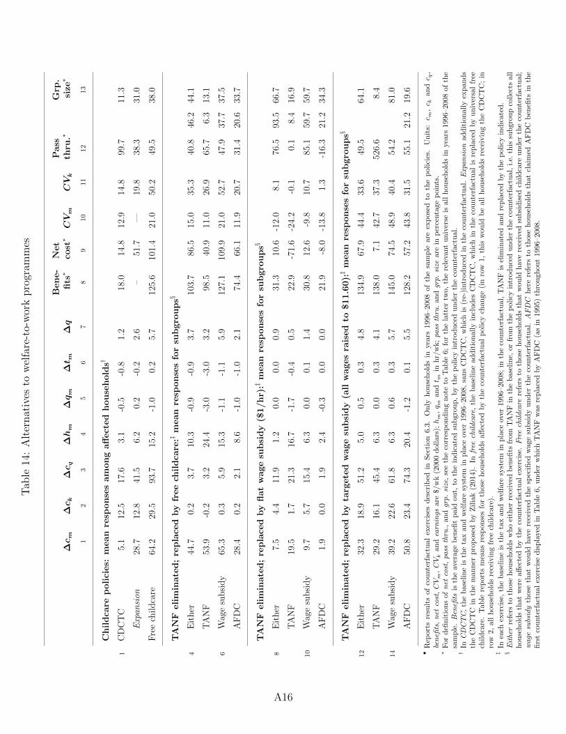
Tab

le14

:A

lter

nat

ives

tow

elfa

re-t

o-w

ork

pro

gram

mes

Ben

e-

Net

Pass

Grp

.∆cm

∆ck

∆cq

∆hm

∆qm

∆t m

∆q

fits∗

cost∗CVm

CVk

thru

.∗si

ze∗

12

34

56

78

910

11

12

13

Ch

ild

care

poli

cies:

mean

resp

on

ses

am

on

gaff

ect

ed

hou

seh

old

s†

1C

DC

TC

5.1

12.5

17.6

3.1

-0.5

-0.8

1.2

18.0

14.8

12.9

14.8

99.7

11.3

Exp

ansi

on28

.712

.841

.56.

20.

2-0

.22.

6–

51.7

—19

.838

.331

.0

Fre

ech

ildca

re64

.229

.593

.715

.2-1

.00.

25.

712

5.6

101.

421

.050

.249

.538

.0

TA

NF

eli

min

ate

d;

rep

lace

dby

free

chil

dca

re:‡

mean

resp

on

ses

for

sub

gro

up

s§

4E

ither

44.7

0.2

3.7

10.3

-0.9

-0.9

3.7

103.

786

.515

.035

.340

.846

.244

.1

TA

NF

53.9

-0.2

3.2

24.4

-3.0

-3.0

3.2

98.5

40.9

11.0

26.9

65.7

6.3

13.1

6W

age

subsi

dy

65.3

0.3

5.9

15.3

-1.1

-1.1

5.9

127.

110

9.9

21.0

52.7

47.9

37.7

37.5

AF

DC

28.4

0.2

2.1

8.6

-1.0

-1.0

2.1

74.4

66.1

11.9

20.7

31.4

20.6

33.7

TA

NF

eli

min

ate

d;

rep

lace

dby

flat

wage

sub

sid

y($

1/h

r):‡

mean

resp

on

ses

for

sub

gro

up

s§

8E

ither

7.5

4.4

11.9

1.2

0.0

0.0

0.9

31.3

10.6

-12.

08.

176

.593

.566

.7

TA

NF

19.5

1.7

21.3

16.7

-1.7

-0.4

0.5

22.9

-71.

6-2

4.2

-0.1

0.1

8.4

16.9

10

Wag

esu

bsi

dy

9.7

5.7

15.4

6.3

0.0

0.1

1.4

30.8

12.6

-9.8

10.7

85.1

59.7

59.7

AF

DC

1.9

0.0

1.9

2.4

-0.3

0.0

0.0

21.9

-8.0

-13.

81.

3-1

6.3

21.2

34.3

TA

NF

eli

min

ate

d;

rep

lace

dby

targ

ete

dw

age

sub

sid

y(a

llw

ages

rais

ed

to$11.6

0):‡

mean

resp

onse

sfo

rsu

bgro

up

s§

12

Eit

her

32.3

18.9

51.2

5.0

0.5

0.3

4.8

134.

967

.944

.433

.649

.564

.1

TA

NF

29.2

16.1

45.4

6.3

0.0

0.3

4.1

138.

07.

142

.737

.352

6.6

8.4

14

Wag

esu

bsi

dy

39.2

22.6

61.8

6.3

0.6

0.3

5.7

145.

074

.548

.940

.454

.281

.0

AF

DC

50.8

23.4

74.3

20.4

-1.2

0.1

5.5

128.

257

.243

.831

.555

.121

.219

.6

•R

eport

sre

sult

sof

counte

rfac

tual

exer

cise

sdes

crib

edin

Sec

tion

6.3

.O

nly

hou

sehold

sin

year

s19

96–2

008

ofth

esa

mple

are

exp

osed

toth

ep

olici

es.

Unit

s:c m

,c k

andc q

,be

nefi

ts,

net

cost

,CVm

,CVk

and

earn

ings

are

$/w

k(2

000

dollars

);hm

,q m

andt m

inhr/

wk;

pass

thru

.and

grp.

size

are

inp

erce

nta

ge

poin

ts.

∗F

or

defi

nit

ions

of

net

cost

,pa

ssth

ru.,

and

grp.

size

,se

eth

eco

rres

pondin

gnot

eto

Table

6;

for

the

latt

ertw

o,th

ere

leva

nt

univ

erse

isall

house

hol

ds

inye

ars

1996

–200

8of

the

sam

ple

.B

enefi

tsis

the

aver

age

ben

efit

paid

out,

toth

ein

dic

ate

dsu

bgro

up,

by

the

policy

intr

oduce

dunder

the

counte

rfact

ual.

†In

CD

CT

C,

the

bas

elin

eis

the

tax

and

wel

fare

syst

emin

pla

ceov

er19

96–2

008,

sans

CD

CT

C,

whic

his

(re-

)intr

oduce

din

the

counte

rfact

ual.

Exp

an

sion

addit

ionally

expan

ds

the

CD

CT

Cin

the

man

ner

pro

pose

dby

Zilia

k(2

014

).In

free

chil

dca

re,

the

base

line

addit

ional

lyin

cludes

CD

CT

C,

whic

hin

the

counte

rfact

ual

isre

pla

ced

by

univ

ersa

lfr

eech

ildca

re.

Tab

lere

por

tsm

eans

resp

onse

sfo

rth

ose

house

hold

saff

ecte

dby

the

counte

rfact

ual

policy

change

(in

row

1,th

isw

ould

be

all

house

hold

sre

ceiv

ing

the

CD

CT

C;

inro

w2,

all

house

hol

ds

rece

ivin

gfr

eech

ildca

re).

‡In

each

exer

cise

,th

ebase

line

isth

eta

xan

dw

elfa

resy

stem

inpla

ceov

er199

6–20

08;

inth

eco

unte

rfact

ual

,T

AN

Fis

elim

inate

dan

dre

pla

ced

by

the

policy

indic

ate

d.

§E

ither

refe

rsto

those

hou

sehol

ds

who

eith

erre

ceiv

edb

enefi

tsfr

om

TA

NF

inth

ebas

elin

e,or

from

the

pol

icy

intr

oduce

dunder

the

counte

rfac

tual

,i.e.

this

subgro

up

collec

tsal

lhouse

hol

ds

that

wer

eaff

ecte

dby

the

counte

rfact

ual

exer

cise

.F

ree

chil

dca

rere

fers

toth

ose

hou

sehol

ds

that

wou

ldhav

ere

ceiv

edsu

bsi

dis

edch

ildca

reunder

the

counte

rfact

ual;

wage

subs

idy

thos

eth

atw

ould

hav

ere

ceiv

edth

esp

ecifi

edw

age

subsi

dy

under

the

counte

rfac

tual

.A

FD

Cher

ere

fers

toth

ose

house

hold

sth

at

claim

edA

FD

Cb

enefi

tsin

the

firs

tco

unte

rfac

tual

exer

cise

dis

pla

yed

inT

able

6,under

whic

hT

AN

Fw

asre

pla

ced

by

AF

DC

(as

in19

95)

thro

ughou

t1996–

2008

.

A16

References for appendices

Bitler, M., and H. Hoynes (2016): “Strengthening Temporary Assistance for Needy Families,”

in Improving Safety Net and Work Support. The Hamilton Project.

Blundell, R., L. Pistaferri, and I. Preston (2008): “Consumption inequality and partial

insurance,” American Economic Review, 98(5), 1887–1921.

Bruins, M., and J. Duffy (2015): “The econometrics of time-use data,” Working paper.

Dunbar, G., A. Lewbel, and K. Pendakur (2013): “Children’s Resources in Collective House-

holds: Identification, Estimation and an Application to Child Poverty in Malawi,” American

Economic Review.

Eslami, E., J. Leftin, and M. Strayer (2012): “Supplemental Nutrition Assistance Program

Participation Rates: Fiscal Year 2010,” Discussion paper, United States Department of Agricul-

ture, Appendix G.

Guryan, J., E. Hurst, and M. Kearney (2008): “Parental Education and Parental Time with

Children,” Journal of Economic Perspectives.

Hoynes, H. (2014): “Proposal 11: Building on the Success of the Earned Income Tax Credit,” in

Improving Safety Net and Work Support. The Hamilton Project.

Ziliak, J. (2014): “Proposal 10: Supporting Low-Income Workers through Refundable Child-Care

Credits,” in Improving Safety Net and Work Support. The Hamilton Project.

A17