tahsin tezdogan*, atilla incecik and osman turan · tahsin tezdogan*, atilla incecik and osman...
TRANSCRIPT

Page | 1
Operability assessment of high speed passenger ships based on human comfort criteria
Tahsin Tezdogan*, Atilla Incecik and Osman Turan
Department of Naval Architecture, Ocean and Marine Engineering, University of Strathclyde, 100 Montrose
Street, Glasgow, G4 0LZ, UK
*corresponding author; e-mail: [email protected], phone: +44(0)1415484912
ABSTRACT
The growing popularity of passenger cruise lines means continual challenges are faced
concerning both a vessel’s design and its operational ability. Vessel dimensions, service
speeds and performance rates are rapidly increasing to keep pace with this expanding interest.
It is essential that vessels demonstrate high performances, even in adverse sea and weather
conditions, and ensure the comfort of passengers and the safety of cargo.
A vessel’s operability can be defined as the percentage of time in which the vessel is capable
of performing her tasks securely. In order to calculate a vessel’s operability index, many key
parameters are required. These include the dynamic responses of the ship to regular waves,
the wave climate of the sea around the ship’s route, and the assigned missions of the vessel.
This paper presents a procedure to calculate the operability index of a ship using seakeeping
analyses. A discussion of the sensitivity of the results relative to three different employed
seakeeping methods is then given. The effect of seasonality on a ship’s estimated operability
is also investigated using wave scatter diagrams. Finally, a high speed catamaran ferry is
explored as a case study and its operability is assessed with regards to human comfort
criteria.
Keywords: Operability, Seakeeping, Passenger Vessels, Human Comfort, Strip Theory,
Potential Theory
1. INTRODUCTION
Recently, a rapid increase has been seen in the number of passengers travelling worldwide by
passenger vessels. Annually, throughout the world, it is estimated that roughly 10 million
people travel on over 230 cruise vessels (Riola and Arboleya, 2006). A key responsibility of
naval architects is to ensure the comfort and well-being of such passengers.
Due to the dynamic nature of a seaway, a vessel’s performance and safety are often disrupted
by enormous dynamic loads, motions and accelerations. Such factors may seriously affect
both the well-being and safety of the passengers and crew, leading to motion sickness and
similar motion-induced forms of discomfort.
For this reason, an operability analysis, considering human comfort criteria, plays a vital role
in ship design, especially for the design of passenger ships -from leisure crafts, to extremely
large cruisers. Considerable investment is made when building a passenger vessel. The
comfort level of the passengers is of paramount importance, and must be maintained above a
specific threshold. This threshold must therefore be continually considered during the design
of a passenger vessel. This should be quantified by applying an operability assessment
procedure invoking seakeeping analyses in accordance with reliable seakeeping criteria.
The major parameters which are required to perform such an operability analysis can be
divided into the following three main categories:
i) vessel geometry and loading condition
ii) definition of the seaway and wave data
Page | 2
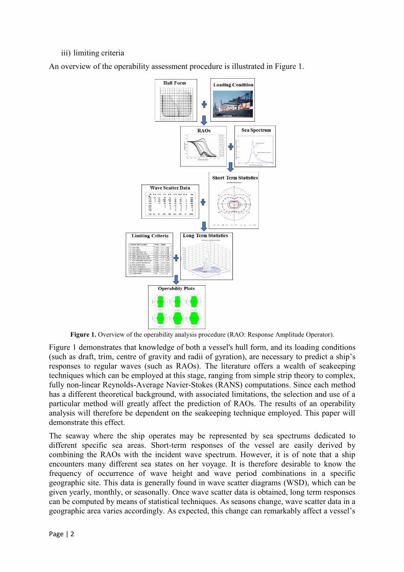
iii) limiting criteria
An overview of the operability assessment procedure is illustrated in Figure 1.
Figure 1. Overview of the operability analysis procedure (RAO: Response Amplitude Operator).
Figure 1 demonstrates that knowledge of both a vessel's hull form, and its loading conditions
(such as draft, trim, centre of gravity and radii of gyration), are necessary to predict a ship’s
responses to regular waves (such as RAOs). The literature offers a wealth of seakeeping
techniques which can be employed at this stage, ranging from simple strip theory to complex,
fully non-linear Reynolds-Average Navier-Stokes (RANS) computations. Since each method
has a different theoretical background, with associated limitations, the selection and use of a
particular method will greatly affect the prediction of RAOs. The results of an operability
analysis will therefore be dependent on the seakeeping technique employed. This paper will
demonstrate this effect.
The seaway where the ship operates may be represented by sea spectrums dedicated to
different specific sea areas. Short-term responses of the vessel are easily derived by
combining the RAOs with the incident wave spectrum. However, it is of note that a ship
encounters many different sea states on her voyage. It is therefore desirable to know the
frequency of occurrence of wave height and wave period combinations in a specific
geographic site. This data is generally found in wave scatter diagrams (WSD), which can be
given yearly, monthly, or seasonally. Once wave scatter data is obtained, long term responses
can be computed by means of statistical techniques. As seasons change, wave scatter data in a
geographic area varies accordingly. As expected, this change can remarkably affect a vessel’s

Page | 3
operability. The paper also argues the effect of seasonality on the expected ship operability in
a comparative manner.
The paper begins with a brief review of the literature on a ship’s operability and seakeeping
methods. Afterwards, an overview of the procedure for operability assessment is presented.
Each stage of the methodology is introduced in detail in the subsequent sub-sections. A high
speed car/passenger ferry operating in the west coast of Scotland is then explored as a case
study, and the operability indices of the vessel are calculated. The results explicitly reveal the
influence of seasonality on the predicted ship operability. The paper also investigates the
sensitivity of the operability index to the adopted seakeeping technique to generate an RAO
database. Finally, all of the results drawn from this work are briefly assessed in the last
section.
2. BACKGROUND
The history of prediction of ship motions starts with Froude’s novel study on rolling (Froude,
1861). Sources such as Newman (1978) and Beck and Reed (2001) can be referred to for a
detailed historical approach to seakeeping.
Two developments in the 1950’s pioneered modern seakeeping computations. The first
development was the proposal of the random process theory to obtain short term responses to
an irregular sea, and the second one was associated with the development of linear ship
motion theories to obtain ship responses to regular waves (Beck and Reed, 2001).
St. Denis and Pierson (1953) pioneered a new method to estimate the statistics of ship
motions in a seaway, which involved the application of spectral methods. This original theory
was based on two fundamental assumptions:
The sea surface has an ergodic Gaussian distribution,
There is a linear relationship between wave elevation, wave loads and ship motions.
The transfer functions can be computed either experimentally or numerically. Experimental
methods are generally used for the validation of numerical results since conducting
experiments for each ship speed and heading would be very expensive and time consuming.
There is therefore a wide range of commercial software available, which can calculate the
RAOs of a desired vessel within a few minutes.
Viscosity is neglected in most seakeeping analyses, meaning that potential theory is still a
very popular technique. However, some empirical viscous corrections are employed in the
potential theory-based methods in an attempt to incorporate viscous effects into the
formulation.
Beck and Reed (2001) estimate that 80% of all seakeeping computations at forward speeds
are still performed using strip theory, because its fast, reliable solutions have sufficient
accuracy for engineering purposes. Another advantage of strip theory is that it is also
applicable to most conventional hull forms. However, discrepancies between strip theory and
experiments for higher speed vessels, or highly non-wall sided hull forms, have motivated
research to develop more advanced theories, such as the 3-D Rankine panel method, unsteady
RANS methods and Large Eddy Simulation (LES) methods (Beck and Reed, 2001).
As discussed by Newman (1978), the conventional strip theory shows deficiencies both for
low encounter frequencies and high speeds, due to assumptions used in the theory. When the
theory is applied to low encounter frequencies, some fundamental problems occur, stemming
from the evolution of forward speed effects and the complex nature of the diffraction problem
in short incoming waves. The conventional strip theory is therefore questionable at low
encounter frequencies and this is visible in the trend of a two-dimensional heave added mass

Page | 4
curve plotted against the frequency of oscillation, as shown in Figure 2. As the frequency of
encounter goes to zero (ωe→0), the added mass coefficients for vertical motions
exponentially become infinite (a→∞). For this reason, strip theory is named a short-
wavelength (high frequency) theory (Beck and Reed, 2001). The other problem strip theory
undergoes is related to forward speed effects. In strip theory, the forward speed has a direct
bearing on the hydrodynamic force due to the simple introduction of terms which are
proportional to (U/ωe) and (U/ωe)2 (where U denotes forward speed). Faltinsen and Zhao
(1991b) also point out that strip theory is the most robust theory when applied at a moderate
forward speed of a vessel, though it is dubious for high speed applications because it models
the interaction with the forward speed in a simplistic way. Furthermore, the effect of the local
steady flow around the vessel is omitted.
Figure 2. Added mass coefficients for a family of 2-D rectangular cylinders, based on the computations of
Vugts (1968), taken from Newman (1978)
(a33: heave added mass, ρ: fluid density, ωe: frequency of encounter, T: draft of the cylinder and B: beam of the
cylinder).
As computers become more powerful, the use of 3-D techniques to investigate seakeeping
problems is more common. Principally, there are two methods to solve three-dimensional
features of seakeeping problems at a forward speed, namely, the Neumann-Kelvin theory
(Brard, 1972 and Guevel et al., 1974) and the Dawson (double-body) method (Dawson,
1977). In the Neumann-Kelvin theory, the body boundary condition is satisfied about the
mean position of the body, and the problem is solved using the free surface Green function
with panels distributed over the mean hull surface. In the Dawson approach, the free surface
linearisation is about the double-body flow, and Rankine source methods are treated with
source distribution over the free surface and the body surface (Wang, 2000, Beck and Reed,
2001).
Yasukawa (2003) claims that 3-D Rankine panel methods have been developed to overcome
the deficiencies in the strip theory methods. He suggests that for a detailed review of Rankine
singularity methods, Bertram and Yasukawa (1996) and Bertram (1998) may be consulted. In
the theory developed by Bertram and Yasukawa (1996), fully 3-D effects of the flow and
forward speed are taken into account, in contrast to strip theory where these effects are not
properly accounted for. Yasukawa (2003) applied the theory of Bertram and Yasukawa
(1996) in the time domain to several container ships with strong flare. As a result of his

Page | 5
validation study, it was found that hydrodynamic forces, ship motions and local pressures are
much better predicted than those obtained by strip theory when compared with experiments.
However, the calculated lateral hydrodynamic forces are not satisfactory, owing to the
viscous flow effect. The author suggests that this problem can be reduced by applying
empirical corrections, similar to those employed in strip theory.
Unfortunately, due to the fact that running a three-dimensional code is a demanding process,
3-D techniques require large amounts of computational power (Hermundstad et al., 1999).
Therefore, a compromise between 2-D and 3-D methods has been made and a new approach
to treat the nonlinear problem in the down-stream direction has been developed. This theory
is the so-called high-speed slender body theory, or 2.5-D theory.
The majority of ship geometries are elongated, with their breadth and draft of the same order
of magnitude relative to the length. This geometric feature is the basis of the slender-body
assumptions, first used in the steady-state wave resistance problem by Cummins (1956).
Another noteworthy restriction from the theory is that the ship is slender compared to the
characteristic incident wavelength. As a consequence of this, the beam and draft are thought
small relative to both the wavelength scale U2/g and the ship length L. Similarly, the Froude
number (Fn=U/(gL)0.5) is assumed to be of order one (g denotes gravitational acceleration).
The slender body theories are therefore termed long-wavelength theories (Newman, 1978).
As explained by Wang (2000), in the slender-body theories, the inner fluid is treated as two-
dimensional, whereas the outer solution for the far-field is treated as three-dimensional. Many
different slender body theories have been developed regarding the different treatments of the
inner two-dimensional problem, such as the original slender body theory (Newman, 1964),
the unified slender body theory (Newman, 1978), the high speed slender body theory
(Chapman, 1975), and the new slender body theory (Yueng and Kim, 1985).
Faltinsen and Zhao (1991a, b), on the other hand, treated the two-dimensional problem by
using a hybrid boundary element method in their high-speed slender body theory. The simple
source-dipole distribution is applied in the inner region, whereas the outer region benefits
from analytical wave-free expressions. By using this method, the important diverging wave
system around a high speed hull is accurately incorporated, whereas the transverse waves,
which are very significant at lower speeds, cannot be included in the theory. Consequently,
this method is only convenient to high speed ships. Numerically, only a side of the vessel is
discretised to decrease computational effort. However, it is still possible to incorporate
hydrodynamic interactions between demi-hulls within the theory. If the hull interaction is not
accounted for, this means the effect of the other demi hull is neglected while calculating the
velocity potential of one hull (Hermundstad et al., 1999).
As discussed by Wang (2000), despite the slender body theory being more rational than the
conventional strip theory from a physical point of view, it is not extensively used due to its
arduous and difficult numerical evaluation of the coefficients. According to real case studies
performed by Sclavounos (1984, 1985) at Fn=0.2 and 0.35, as the exciting force is calculated
more accurately in the slender-body theories, the ship motion predictions are not significantly
better than those from the linear strip theory. Also, it is revealed by ITTC (1987) that the
slender body theory gives no advantage over the strip theory for predicting a ship's vertical
motions at forward speed, though it does demonstrate advantages for the prediction of sway
and yaw motions.
As mentioned above, there are several methods to determine the response operators. Each
technique features different assumptions and limitations, and therefore the output from a
given technique will have a significant impact on the operability calculations. In order to

Page | 6
highlight this problem, three particular methods will be employed to estimate the RAOs of
the ferry. These are:
Theory 1: Conventional strip theory formulation (2-D)
Theory 2: High-speed formulation in which hull interaction is not included (2½-D)
Theory 3: High-speed formulation in which hull interaction is included (2½-D)
In order to apply these theories in the operability calculations, VERES, which is based on a
linear, potential, strip theory software package, is used in this study (Fathi, 2004). The fluid is
assumed to be homogeneous, non-viscous, irrotational and incompressible. However, viscous
roll damping is taken into account in this seakeeping package, employing some empirical
formulae. For more information, the theory manual of the software can be consulted (Fathi
and Hoff, 2013).
Theory 1 is based on the strip theory formulation by Salvesen, Tuck and Faltinsen (1970),
which is particular to low ship speeds. The restrictions of this theory were explained above.
Theory 2 is based on a strip theory approach of Faltinsen and Zhao (1991a) and Faltinsen et
al. (1991, 1992), and is briefly explained by Fathi and Hoff (2013): “The high-speed
formulation is based on a strip theory approach, where the free-surface condition is used to
step the solution in the downstream direction. The solution is started assuming that both the
velocity potential and its x-derivative are zero at the first strip, counted from the bow”. Hoff
(2014) describes the principal difference between the traditional strip theory and the high
speed formulation as that both formulations solve a two dimensional problem for each strip,
but only the high speed formulation accounts for the interaction between the solutions of each
strip by stepping the solution in the downstream direction.
In Theory 3, the forces exerted on the ship are directly calculated from the velocity potentials,
employing integral theorems, similar to Theory 1. In the high speed formulation without hull
interaction (Theory 2), the forces are calculated by integration of the pressure over the hull
surface. Hermundstad et al. (1999) has found that these two methods (Theory 2 and 3) result
in differences in the calculated heave and pitch motions; particularly around resonance.
There is wave interference between the waves generated by each single hull of a catamaran.
Faltinsen (2005) defines this wave interference as follows “the waves generated from each
hull are superimposed without accounting for the fact that the waves generated by one hull
will be modified because of the presence of another hull”. The waves generated by one hull
may become incident to another demihull, causing wave diffraction to occur. In the theory, a
first assessment to determine whether any wave interaction is expected between the two side
hulls of a catamaran can be performed by assuming there is no hydrodynamic hull
interaction. The wave angle (αc), given by Eq. 1, can then be calculated, to determine whether
the waves inside the wave angle become incident to the other hull. It should also be
highlighted that Theory 3 is capable to account for this diffraction effect occurring between
the demihulls of a catamaran (Faltinsen, 2005).
tan2
c
e
g
U
(1)
1 1 20.51 2 eUL b b
L L g
(2)
where b2 is the beam of a single hull and b1 is the distance between hull sides, as shown in
Figure 3. L is the ship length and L1 is the length of the aft part of the side which is affected
by the other hull. Throughout this paper, ωe denotes the frequency of encounter and
gravitational acceleration g is taken as 9.81 m/sec2.

Page | 7
Figure 3. Hull interaction in a catamaran due to the wave effect, taken from Faltinsen (2005).
Each of the methods explained above will be used to independently calculate the motion
responses of the ferry to regular waves, for a range of wave headings, to predict its
operability. It should be stated that a 0° wave headings (β=0°) corresponds to a head sea
condition in this paper.
Operability and habitability assessments have been conducted for a variety of ship types by
many researchers. Some of their conclusions have had an impact on operability analyses of
passenger ships, specifically with regards to human comfort. O’Hanlon and McCauley (1974)
and McCauley et al. (1976) conducted simulation trials to investigate motion sickness caused
by a ship’s vertical sinusoidal motions. Their work was then combined with seakeeping
analysis techniques (Salvesen et al. 1970, McTaggart 1997), leading to the development of
several suitable methods for the operability analysis of passenger ferries.
Ikeda et al. (1991) proposed a method to estimate the ratio of motion sick people on-board a
ferry, by combining strip theory with O’Hanlon and McCauley’s (1974) research. The
operational performance of passenger ferries was evaluated by Dallinga et al. (2002)
considering the influence of the motion sickness on passengers and crew. In addition, Sarioz,
K. and Sarioz, E. (2005) investigated the effect of limiting criteria on the seakeeping
performance assessment for passenger vessels and concluded that the expected seakeeping
performance of a passenger vessel is entirely related to the magnitude of the defined limiting
criteria. They evaluated habitability of the passenger vessel based solely on vertical
accelerations defined by the ISO 2631/3 standard (ISO, 1985). Tezdogan et al. (2013) also
presented operability analyses of two high speed car/passenger ferries. RAO databases of the
crafts were generated using 2.5-D high speed theory. Their study explored the optimal vessel
configuration and loading condition, with regards to operability.
Several researchers have carried out operability analyses on other ship types. Soares et al.
(1995) offered a simple procedure for the seakeeping performance assessment of a fishing
vessel. Then, Fonseca and Soares (2002) proposed a methodology to assess the seakeeping
performance of vessels and argued the sensitivity of the results in relation to the use of
various limiting criteria. They also revealed the influence of seasonality on the ship
operability by comparing winter statistics to the annual statistics. The calculation of
operability indices and the sensitivity analyses were performed for both a container ship and a
fishing vessel in their study. Mortola et. al (2012) proposed an operability evaluation
methodology and developed a decision-making support tool to rapidly assess and compare
the operability of the two candidate vessels, to provide an operational and maintenance
support service to offshore wind farms.

Page | 8
3. METHODOLOGY
The methodology towards the prediction of the operability of ships is briefly presented in this
section.
The operability assessment technique typically begins with the calculation of motion
characteristics of the given ship for all headings at the sea area which is particular to the
vessel’s course. Then, these responses (RAOs) are combined with the wave spectrum to
predict the short-term responses to irregular seas. Next, limiting significant wave heights are
calculated for each seakeeping criterion by utilising the short term responses. Finally, the
calculation of the operability index, which is the percentage of the number of wave height
and wave period combinations not violating the predetermined criteria, can be computed
taking into account long term statistics of the wave data.
A high speed catamaran car/passenger ferry is used in this paper as a case study to argue the
effect of the various methods to predict RAOs. The main characteristics and geometry of the
ferry are given in Table 1 and Figure 4, respectively.
Table 1. Main characteristics of the catamaran ferry (Tezdogan et al., 2013).
Length between perpendiculars (LBP) 151.12 m
Overall beam of twin-hull (BOA) 36.72 m
Beam of demi-hull (BDH) 10.68 m
Design draught (T) 9.4 m
Displacement (Δ) 16,448 m3
Hull centre line spacing 26.04 m
Longitudinal centre of gravity (LCG) aft of amidships 11.84 m
Vertical centre of gravity (VCG) from the base line 13.28 m
Pitch radius of gyration (r55) 39.24 m
Roll radius of gyration (r44) 13.36 m
Yaw radius of gyration (r66) 40.88 m
Design speed (U) 20 knots
The Marintek Catamaran is taken as a ship model and has been scaled to real ship
dimensions. All details related to the catamaran model can be found in Hermundstad et al.
(1999).
Figure 4. Sections of a demihull
(left and right hand sides of the graph show aft and forward stations, respectively).
Although the demi-hulls of the catamaran geometry are connected to each other above the
water line, only the sections under the free surface have been shown in Figure 4.
All of the necessary stages to predict the operability of the vessel are briefly explained in the
following sub-sections.

Page | 9
3.1. Ship responses to regular waves
Typically, the first stage in the assessment of a ship’s operability is to predict the ship
response characteristics in regular waves for a range of headings and ship speeds in the
frequency domain. The transfer functions (RAOs) are usually calculated due to either a unit
wave amplitude elevation for translational motions, or a unit wave slope amplitude for
angular motions.
The numerical RAOs of the ferry, obtained by using each theory, are compared to the
experimental data published by Hermundstad et al. (1999). Four different combinations of
ship speed and wave heading are presented below, being identified by their case numbers.
Case 1: Froude number 0.47 (corresponds to a forward speed of 35.18 knots). Head
seas.
Case 2: Froude number 0.63 (corresponds to a forward speed of 47.16 knots). Head
seas.
Case 3: Froude number 0.63. Bow seas (β=30°).
Case 4: Froude number 0.47. Beam seas (β=90°).
The comparisons are shown in Figures 5-8, representing the experimental results using
triangles. Heave responses are non-dimensionalised by wave amplitude (A), whereas pitch
and roll responses are non-dimensionalised by wave amplitude over ship length (A/LBP). It is
worth noting that the angular responses are given in radians. The graphs, demonstrated in
Figures 5-8, are all plotted against non-dimensional wave frequency, ω'=ω(LBP/g)1/2.
Figure 5. Experimental and numerical RAOs for Case 1. Left and right hand sides of the graph show heave and
pitch RAOs, respectively.
Figure 6. Experimental and numerical RAOs for Case 2. Left and right hand sides of the graph show heave and
pitch RAOs, respectively.

Page | 10
Figure 7. Experimental and numerical RAOs for Case 3. Upper left and right hand sides of the graph show
heave and pitch RAOs, respectively. Lower part shows roll RAOs.
Figure 8. Experimental and numerical RAOs for Case 4. Left and right hand sides of the graph show heave and
roll RAOs, respectively.
Figures 5-8 appear to demonstrate the discrepancies between each numerical technique and
the experimental results. If Theory 2 is compared to Theory 3, it is evident from Figures 6
and 7 that the numerical calculation of the resonant heave motion is improved when hull
interactions are taken into account. In most cases, Theory 3 shows better agreement with the
experimental data relative to Theory 2. This applies to both head and bow seas. It is worth
noting that hull interactions are more dominant in heave motion compared to pitch motion at
two high speeds. Conversely, for the roll motions, the discrepancies are much larger when
hull interactions are taken into consideration. In most cases, of the three theories,
conventional strip theory (Theory 1) is still the most compatible with the experiments, as this
shows consistency with the ITTC (1987)’s conclusion, explained in the previous section.
Given that wave frequency equals the encounter frequency in beam seas, it is more
convenient to compare the natural roll frequency of the vessel with the peak frequencies
obtained by each numerical result in Figure 8. The natural roll frequency of the vessel
(ωroll=0.96 rad/sec), which coincides with ω'roll=3.77, is very close to the peak frequency
estimated by both Theory 1 and 2 (ω'p=3.79), followed by Theory 3 (ω'p=3.34) in beam seas.

Page | 11
Furthermore, the effects of three-dimensional flow, viscosity and nonlinearities are neglected
in all three methods. This therefore causes an increase in the discrepancies between the
numerical analyses and experiments (Hermundstad et al., 1999).
The sensitivity of the expected operability by using different theories to generate RAOs will
be explored in the next section.
Additionally, a comparison of the vertical accelerations at the centre of gravity (CG) by
means of the different theories in head seas at 20 knots ship speed (Fn= 0.267) is given in
Figure 9. The abscissa of the figure is encounter frequency, whereas the ordinate is vertical
acceleration, non-dimensionalised by gA/LBP, conforming with the ITTC guideline (ITTC,
2011).
Figure 9 clearly demonstrates discrepancies between the vertical accelerations using different
theories, particularly when applied to the resonance heave frequency (natural heave
frequency of the vessel ωheave=1.184 rad/sec). The RAO vertical acceleration calculated using
Theory 3 is 4.18 and 2.18 times higher than that obtained by Theory 1 and 2 in the resonance
frequency, respectively. Vertical acceleration by means of Theory 3 gives higher results
because of the effect of wave interactions between each demihull. This will be discussed in
detail in the following paragraphs. If Theory 1 is compared to Theory 2, the differences in the
vertical acceleration around the resonance frequency arise from the evaluation of forward
speed in the free surface condition.
Figure 9. Vertical acceleration RAOs at the centre of gravity against encounter frequency in head seas at 20
knots speed.
Typical vertical acceleration RAOs in head seas as a function of wave frequency and ship
service speed, calculated using Theory 1, 2 and 3, are shown in Figures 10-12, respectively.

Page | 12
Figure 10. Vertical acceleration RAOs at the centre of gravity in head seas, calculated using Theory 1 at a
range of forward speeds.
Figure 11. Vertical acceleration RAOs at the centre of gravity in head seas, calculated using Theory 2 at a
range of forward speeds.

Page | 13
Figure 12. Vertical acceleration RAOs at the centre of gravity in head seas, calculated using Theory 3 at a
range of forward speeds.
Figures 10-12 demonstrate that vertical acceleration RAOs obtained using Theory 1 and 2 are
very similar to each other, showing a gradual increase with increasing speed. Conversely,
vertical accelerations generated using Theory 3 (Figure 12) show a different trend. They
decrease with increasing speed between a speed range of 18-21 knots, and after this particular
range they gradually increase with increasing speed, showing an expected trend. This is due
to the fact that hydrodynamic hull interactions are most significant within a speed range of
18-21 knots for the ferry in question, and the waves generated by each demihull affect the
vertical accelerations. According to Eq. 2, for a given frequency of encounter, the wave
interaction between demihulls decreases as ship speed increases. This clearly explains why
the vertical accelerations obtained using Theory 3 show a reversed trend between this
particular speed range.
Table 2 presents L1/L ratios (based on Eq. 2) against a range of wave frequencies, for varying
forward speeds of the ferry.
Table 2. L1/L ratios of the ferry, calculated based on Eq. 2, for a range of ω at different speeds.
ω
(rad/s)
Ship forward speed, U (knots)
18 19 20 21 22 23 24 25 26 27 28 29 30
0.1 0.97 0.97 0.97 0.97 0.97 0.96 0.96 0.96 0.96 0.96 0.95 0.95 0.95
0.2 0.94 0.93 0.93 0.93 0.92 0.92 0.91 0.91 0.91 0.90 0.90 0.89 0.89
0.4 0.86 0.85 0.84 0.83 0.82 0.80 0.79 0.78 0.77 0.76 0.75 0.73 0.72
0.6 0.76 0.74 0.72 0.70 0.68 0.66 0.64 0.62 0.59 0.57 0.55 0.52 0.50
0.8 0.64 0.61 0.58 0.55 0.51 0.48 0.45 0.41 0.38 0.34 0.30 0.26 0.22
1.0 0.50 0.46 0.41 0.37 0.32 0.27 0.22 0.17 0.12 0.06 0.01 [ ] [ ]
1.2 0.34 0.28 0.22 0.16 0.10 0.03 [ ] [ ] [ ] [ ] [ ] [ ] [ ]
1.4 0.16 0.08 0.01 [ ] [ ] [ ] [ ] [ ] [ ] [ ] [ ] [ ] [ ]
Empty brackets [ ] indicate that there is no applicable hull interaction. Table 2 shows that the
length L1 decreases as the wave frequency increases, in other words the L1/L ratio decreases

Page | 14
with decreasing wavelength. It is evident that the hull interaction is most significant in low
encounter frequencies at relatively lower ship speeds.
3.2. Ship responses to irregular waves
The real seaways can only be modelled by virtue of a statistical model. Ship responses to
natural irregular seas (Sz) are calculated by the linear superposition principle, using the
seaway spectrum (Sζ) and the transfer functions in the frequency domain as given below.
2( ) ( ) ( )zS S RAO (3)
Several spectral formulations are available in the literature. One of the most frequently used
spectrums is the JONSWAP spectrum, which was developed in 1973 by the Joint North Sea
Wave Project and described by Hasselmann et al. (1973). The JONSWAP formulation has
been adopted for the fetch limited North Sea and can be expressed as follows:
2
2 24 exp2
2
5
5( ) .exp .
4
p
ppgS
(4)
where ω and ωp are the incident wave and modal wave periods, respectively. σ represents the
spectral width parameter and is calculated according to the following expression:
0.07
0.09
p
p
γ refers to the peak-enhancement factor and is generally taken to be 3.30. α is the
normalisation factor, given by
4 2 45.061(2 ) 1 0.287ln( )s pH (5)
The JONSWAP parametric spectrum is chosen for this study. The spectral density
distribution of the spectrum for Hs=3.5m is illustrated in Figure 13.
Figure 13. Spectral density distribution of the JONSWAP spectrum for Hs=3.5m.

Page | 15
The response spectrum Sz(ω) is the product of the defined sea spectrum Sζ(ω) and square of
the transfer function RAO2(ω) as given in Eq. 3. Once the response spectrum is obtained, all
statistical values of the response are derived by using the spectral technique.
The variance of the response spectrum is the area under the spectrum curve with respect to
natural wave frequency and can be shown by:
00
( )zm S d
(6)
The square root of Eq. 6 gives the root mean square (RMS) of the response, which describes
the most frequently observed amplitude of the waves or responses.
0RMSx m (7)
in which m0 is the zeroth spectral moment. Principally, the nth order spectral moment can be
presented by
0
( )n
n zm S d
(8)
The square roots of the m2 and m4 spectral moments correspond to RMS velocity and
acceleration responses, respectively.
3.3. Determination of the limiting significant wave heights
Soares et al. (1995) suggest that the wave spectrum can be represented as the product of the
normalised wave spectrum in terms of the significant wave height Sζ1(ω) and square of the
significant wave height Hs due to the linearity assumption.
2 2
1( , , ) ( ,1, ) ( , )s s s s s sS H T H S T H S T (9)
By analogy to equation (9), the response spectrum may also be formulated as:
2 2 2
1 1( ) ( ) ( , ) ( )z s z s sS H S H S T RAO (10)
and the variance of the response can be given by:
2 2
0 1
0 0
( ) ( , ) ( )z s sm S d H S T RAO d
(11)
which can briefly be symbolised as follows:
2
0 01sm H m (12)
For cases in which a seakeeping criterion is defined as a root mean square of a response xRMS,
the limiting significant wave height for a specific modal wave period Ts, and ship heading β
is determined by using the following equation:
limlim
,1
( , ) RMSs s
RMS
xH T
x (13)
3.4. Calculation of the operability index
Fonseca and Soares (2002) define the operability index as “the percentage of time during
which the ship is operational”. The operability index is calculated according to the following
common expression, which was also used in Khalid et al. (2009):
(14)
lim
,
,
( )
Op.(%)= 100s s
ss s s
H T
n H H
xN

Page | 16
With regards to Eq. 14 the operability index is the ratio of the number of waves (for all
available zero crossing periods) with significant wave heights not exceeding the maximum
significant wave height (nss,β) relative to the total number of waves (N) in the wave scatter
diagram of interest.
4. OPERABILITY ANALYSIS
The procedure presented in the previous sections can be used to evaluate ship motions and
motion-related responses to both regular waves and irregular seaways. Short term and long
term statistics are obtained in irregular seas to predict the most probable maximum values of
the ship responses. On the other hand, if these results are evaluated alone, they cannot
properly express the performance of a ship from a seakeeping point of view. An operability
index which is capable of measuring the degradation of the ship’s performance to accomplish
her tasks should be computed to quantify the seakeeping ability of the vessel (Fonseca and
Soares, 2002).
4.1. Selection of the limiting criteria
In order to calculate the operability index of the ferry, the limiting criteria should be defined
concerning passenger comfort and safety. A passenger ship’s seakeeping performance
depends partly on lateral accelerations, but mostly on vertical accelerations (Riola and
Arboleya, 2006).
The influence of the vertical acceleration on human metabolism is the major reason for sea-
sickness. Discomfort regions are determined by the International Standard as a function of
acceleration levels, frequencies, and exposure times. There are some parameters to quantify
the effects of accelerations on human performance on-board. They may be regarded as a good
reference to compare the human performance between ship designs (Giron et al., 2001).
The International Standard ISO 2631/1 (ISO, 1997) presents an approach to measure whole-
body vibration in connection with human health and comfort, relating this to the probability
of vibration and motion sickness incidence.
Motion Sickness Incidence (MSI) and Motion Induced Interruptions (MII) are the two most
highly referenced parameters to quantify the ship motion effects on human performance and
comfort. MSI indicates the percentage of people experiencing vomiting when exposed to
motion for a certain of time. It was proposed as a function of the wave frequency and vertical
acceleration by O’Hanlon and McCauley (1974), following which a mathematical expression
was developed by McCauley et al. (1976).
Graham (1990) developed the motion induced interruption concept, which is defined as the
number of loss-of-balance events that occur during an arbitrary operation on-board. The
theory, which is explained in detail in his study, is based on the calculation of the lateral force
estimator (LFE) which causes objects to topple or slide, and people to lose their balance, in
the frequency domain. Graham concluded that a limit on the number of MIIs can be applied
as the most appropriate criterion for deck operations. Table 3 presents the proposed values in
terms of different risk levels.

Page | 17
Table 3. MII risk levels (Graham, 1990).
Risk level MIIs per minute
1. Possible 0.1
2. Probable 0.5
3. Serious 1.5
4. Severe 3.0
5. Extreme 5.0
The derived transfer functions are normally calculated with respect to specific positions on
the ship which are closely associated with the limiting criteria to be used. Table 4 lists these
locations on the ship and the seakeeping criteria that are selected for the operability
assessment of the ferry. The locations in Table 4 are given according to x, y, and z
coordinates, where x denotes the point forward after aft peak, y denotes the position off
centre (positive starboard), and z denotes the location above the base line.
Table 4. Seakeeping criteria for the high speed passenger ferry.
Description Criterion Location Coordinates (m) Reference
Vertical
acceleration
2 hours exposure
0.05g
Passenger deck 80, 0, 10 ISO 2631/3,
1985
MII 0.5 MII per minute Car deck 150, 0, 11 Graham,
1990
MSI 35% MSI in 2 hours Crew
accommodation
25, -4, 9.5 ISO 2631/1,
1997
Lateral
acceleration
0.025g (RMS) Centre of
gravity
63.72, 0, 13.28 ISO 2631/1,
1997
4.2. Definition of the sea spectrum and wave scatter data
It is assumed that the car/passenger ferry provides a fast transportation service across the west
coast of Scotland (Figure 14, Global Wave Area 10).
As outlined earlier on, the JONSWAP spectrum has been selected to represent the area of
operation. In order to determine the long term responses of the vessel, the probability of
occurrence of the sea states at the operation area is necessary. WSD provides such
information as it gives a joint probability table of significant wave heights, characteristic
wave periods, and the number of occurrences for a specific sea site. The statistics of ocean
wave climates for the entire globe is available in Global Wave Statistics for a specific area
based on instrumental, hindcasting, and visual observation methods (Hogben et al., 1986).
The operability calculations are performed using annual and seasonal WSD. Figure 15
depicts the wave scatter data of Area 10 using annual and seasonal statistics for the wave
climate. The bars in the graphs demonstrate the number of waves observed in that
combination of significant wave height and wave period.
According to Lloyd (1989), for ship design purposes the most common practice is to use
short crested sea with a 90° spreading angle, hence the problem is treated in this fashion.
Figure 16 shows the percentage of time variances of significant wave heights observed in
Area 10 with regards to annual and seasonal wave statistics.

Page | 18
Figure 14. Global wave statistics coastal areas (Luis et al., 2009).
Figure 15. Wave scatter data of Area 10 regarding seasonal and annual statistics (Hogben et al., 1986).

Page | 19
Figure 16. Percentage of time variances of significant wave heights observed in Area 10 over various
durations.
5. RESULTS
5.1 Motion sickness incidence
The operability indices will be calculated in this work based on human comfort-oriented
criteria. Beyond any doubt, motion sickness incidence is one of the most important criteria
used to quantify human comfort due to motion in any vessel (car, train, ship). Special
attention will therefore be paid to investigate MSI features of the vessel.
In this sub-section, MSI values of the ferry at the crew accommodation location will be
calculated using the three different theories. MSI values are determined according to ISO
2631/1 (1997) using the following formulae:
0.5
2 1.5
0
( ) /
T
z wfMSDV a t dt m s
(15)
. %m zMSI K MSDV (16)
where MSDVz stands for Motion Sickness Dose Value in the vertical direction. awf is the
frequency-weighted acceleration. The integration time T varies between 20 min and 6 hours
and is taken as 2 hours in this work. Km is a constant in the formula and is taken as 1/3, which
indicates a mixed population of unadapted male and female adults. For more information
about how to predict MSI values, reference can be made to ISO 2631/1 (1997).
In order to be able to predict the MSI values of the vessel in any sea state, the statistical
parameters based on the annual sea state occurrences in the open ocean Northern
Hemisphere, given in Table 5, will be used.

Page | 20
Table 5. Annual sea state occurrences in the open ocean Northern Hemisphere (Bales, 1982)
Sea State
No
Significant
wave
heights
[metres]
Sustained
wind speed
[knots]
Modal wave
period
[seconds]
Percentage
probability
of sea state
2 0.30 8.5 7 5.7
3 0.88 13.5 8 19.7
4 1.88 19.0 9 28.3
5 3.25 24.5 10 19.5
6 5.00 37.5 12 17.5
7 7.50 51.5 14 7.6
According to the data presented in Table 5, sea state 4 is the most frequently seen sea state,
with a probability of 28.3%. On the other hand, sea states 2 and 7 are the least frequently
observed sea states in this geographic area of interest, with probabilities of 5.7% and 7.6%,
respectively.
The MSI values of the ferry are predicted for various sea states at a ship speed of 20 knots.
The significant wave height and modal wave period data, used in the JONSWAP spectrum,
are shown in Table 5. The calculated MSI values using each theory are compared in Figure
17.
Figure 17 demonstrates the differences in MSI values using each theory. Higher sea states
cause higher MSI values, as clearly seen in the figure. Also, it is evident that in the low sea
states (sea states 2-4), the MSI results from each theory appear similar to each other, however
in the high sea states, the discrepancies become significant. Theory 3 gives the highest
results, whereas Theory 1 gives the lowest result in the high sea states. This is as expected
since the vertical accelerations at 20 knots ship speed demonstrate the same trend, as shown
in Figure 9.
Figure 17. Motion sickness incidences calculated using each theory for varying sea states.

Page | 21
5.2 Limiting significant wave heights
The methodology presented in the third section is applied to the ferry to measure the
seakeeping performance of the vessel in terms of its operability index. All calculations have
been carried out at a forward speed of 20 knots.
The limiting significant wave heights are calculated based on each criterion as a function of
peak wave periods for a range of wave headings using Theory 1, 2, and 3 independently. The
results are displayed in Figures 18-20, respectively.
Figure 18. Limiting significant wave heights calculated using Theory 1 for various wave headings.

Page | 22
Figure 19. Limiting significant wave heights calculated using Theory 2 for various wave headings.

Page | 23
Figure 20. Limiting significant wave heights calculated using Theory 3 for various wave headings.
A comparison of the limiting significant wave heights in head seas for each criterion is
displayed in Figure 21. This clearly illustrates the influence of the employed theories on the
maximum allowed significant wave heights. It is seen from the figure that the differences in
the limiting significant wave heights obtained using each theory are most pronounced in the
vertical acceleration criterion. This will lead to noticeable discrepancies in the resultant
operability indices due to vertical acceleration.

Page | 24
Figure 21. Effect of the employed theories on the limiting significant wave heights.
5.3 Operability indices
Operability calculations have been performed, individually, using each theory. The indices
for the car/passenger ferry, resulting from these calculations, are summarised in Table 6,
which includes both annual and seasonal wave statistics for Area 10, across several headings.
In the main columns of the table, the operability indices satisfying each limiting criterion are
shown, independently. The overall indices, which decide whether a vessel satisfies all the
limiting criteria of interest, are calculated by taking the minimum values of each operability
index, and are given on the right-hand block of columns. The average values, which are
presented in the bottom row of each table, are calculated by taking the average of the
operability indices in each wave heading. It is based on the assumption that each wave
heading has an equal probability of occurrence. Using this set of average outputs, the
operability results can be compared with each other more efficiently, regardless of the wave
heading.
The average annual, spring, summer, autumn and winter operability indices for the ferry are
86.15%, 88.67%, 91.61%, 85.80% and 83.43%, respectively, when calculated using Theory
3. The results show that the ship is operational, satisfying all necessary criteria, during
86.15% of a year, on average. A more detailed breakdown for each season is also provided,
for example the ship is, on average, operational 83.43% of the time during winter. When
Theory 1 is used to generate RAOs, these indices increase to 95.21%, 96.46%, 98.60%,
94.73%, and 93.39%. Using Theory 2, the results alter to 93.80%, 95.28%, 97.92%, 93.31%,
and 91.42%, respectively.
As Table 6 shows, the operability is generally small in head and bow seas due to the vertical
acceleration at the fore perpendicular. The vessel’s operability is highest in following or
quarter seas.
It is interesting to note that the overall performance of the vessel is mainly determined by the
vertical acceleration. Also, the operability indices calculated solely with regards to the

Page | 25
vertical acceleration criterion show a remarkably strong dependence on the chosen theory. It
should be kept in mind that operability, as a function of limiting criteria, is dependent of
predetermined criteria. If the selected threshold values given in Table 4 were lowered, it is
obvious that the resultant operability indices would undergo far greater changes when using
the employed theories.
Table 6. Operability indices for the car/passenger ferry operating in Area 10.
Year SpringSummerAutumn Winter Year SpringSummerAutumn Winter Year SpringSummerAutumn Winter Year Spring SummerAutumn Winter Year Spring Summer Autumn Winter
0 90.42 92.62 97.15 89.45 84.40 97.30 98.12 99.52 96.83 95.73 98.22 98.92 99.78 97.97 97.28 99.72 99.92 100 99.72 99.66 90.42 92.62 97.15 89.45 84.40
30 90.81 92.98 97.23 89.88 86.06 95.67 96.88 99.03 95.06 94.04 98.37 99.07 99.84 98.20 97.89 98.68 99.32 99.92 98.62 98.57 90.81 92.98 97.23 89.88 86.06
60 93.19 94.98 98.05 92.46 91.61 94.14 95.76 98.39 93.50 93.23 98.86 99.37 99.93 98.80 98.96 95.34 96.68 98.79 94.76 94.29 93.19 94.98 98.05 92.46 91.61
90 97.22 98.20 99.37 97.09 98.20 95.91 97.25 98.90 95.60 96.59 99.70 99.91 100 99.70 99.91 94.39 96.02 98.25 93.76 93.64 94.39 96.02 98.25 93.76 93.64
120 99.91 100 100 99.91 100 99.08 99.49 99.91 99.07 99.71 100 100 100 100 100 97.65 98.61 99.52 97.54 98.03 97.65 98.61 99.52 97.54 98.03
150 100 100 100 100 100 100 100 100 100 100 100 100 100 100 100 100 100 100 100 100 100 100 100 100 100
180 100 100 100 100 100 100 100 100 100 100 100 100 100 100 100 100 100 100 100 100 100 100 100 100 100
Average 95.94 96.97 98.83 95.54 94.32 97.44 98.21 99.39 97.15 97.04 99.31 99.61 99.94 99.24 99.15 97.97 98.65 99.50 97.77 97.74 95.21 96.46 98.60 94.73 93.39
Year SpringSummerAutumn Winter Year SpringSummerAutumn Winter Year SpringSummerAutumn Winter Year Spring SummerAutumn Winter Year Spring Summer Autumn Winter
0 86.01 88.90 94.86 85.07 78.28 96.00 97.08 99.20 95.34 93.46 98.06 98.66 99.70 97.69 96.36 99.67 99.87 100 99.67 99.60 86.01 88.90 94.86 85.07 78.28
30 87.32 90.04 95.48 86.38 81.15 93.52 95.19 98.26 92.78 91.17 98.37 98.98 99.80 98.13 97.28 98.51 99.21 99.88 98.44 98.45 87.32 90.04 95.48 86.38 81.15
60 91.57 93.69 97.40 90.76 89.27 92.51 94.49 97.77 91.75 90.89 99.04 99.53 99.96 99.00 98.95 95.03 96.46 98.64 94.44 94.07 91.57 93.69 97.40 90.76 89.27
90 96.68 97.82 99.19 96.53 97.84 95.30 96.74 98.64 94.88 95.78 99.83 99.96 100 99.82 99.92 94.20 95.85 98.19 93.55 93.41 94.20 95.85 98.19 93.55 93.41
120 99.88 99.98 100 99.88 100 99.07 99.48 99.91 99.07 99.69 100 100 100 100 100 97.52 98.49 99.49 97.38 97.83 97.52 98.49 99.49 97.38 97.83
150 100 100 100 100 100 100 100 100 100 100 100 100 100 100 100 100 100 100 100 100 100 100 100 100 100
180 100 100 100 100 100 100 100 100 100 100 100 100 100 100 100 100 100 100 100 100 100 100 100 100 100
Average 94.49 95.78 98.13 94.09 92.36 96.63 97.57 99.11 96.26 95.86 99.33 99.59 99.92 99.23 98.93 97.85 98.55 99.46 97.64 97.62 93.80 95.28 97.92 93.31 91.42
Year SpringSummerAutumn Winter Year SpringSummerAutumn Winter Year SpringSummerAutumn Winter Year Spring SummerAutumn Winter Year Spring Summer Autumn Winter
0 66.39 71.36 80.26 65.93 56.92 93.87 95.45 98.39 93.12 91.23 97.39 98.15 99.56 96.84 95.05 99.60 99.82 100 99.60 99.55 66.39 71.36 80.26 65.93 56.92
30 68.86 73.84 81.62 68.40 61.58 92.32 94.23 97.81 91.50 89.34 97.79 98.51 99.65 97.38 96.18 98.29 99.03 99.84 98.20 98.29 68.86 73.84 81.62 68.40 61.58
60 78.88 83.21 88.72 78.21 76.26 90.42 92.82 96.73 89.57 87.96 98.83 99.41 99.93 98.76 98.69 93.80 95.55 97.95 93.15 93.08 78.88 83.21 88.72 78.21 76.26
90 93.34 95.28 97.62 92.80 94.39 92.79 94.79 91.62 92.12 92.38 99.83 99.97 100 99.83 99.93 92.27 94.42 96.82 91.61 92.05 92.27 94.42 91.62 91.61 92.05
120 99.60 99.75 99.95 99.60 99.95 97.58 98.47 99.52 97.52 98.68 100 100 100 100 100 96.69 97.88 99.05 96.48 97.21 96.69 97.88 99.05 96.48 97.21
150 100 100 100 100 100 100 100 100 100 100 100 100 100 100 100 100 100 100 100 100 100 100 100 100 100
180 100 100 100 100 100 100 100 100 100 100 100 100 100 100 100 100 100 100 100 100 100 100 100 100 100
Average 86.72 89.06 92.59 86.42 84.16 95.28 96.54 97.72 94.83 94.23 99.12 99.43 99.88 98.97 98.55 97.24 98.10 99.10 97.01 97.17 86.15 88.67 91.61 85.80 83.43
All criteria
Heading
(deg)
Heading
(deg)
Vertical Acceleration MII MSI
Vertical Acceleration MII MSI Lateral Acceleration All criteria
Heading
(deg)
Vertical Acceleration MII MSI Lateral Acceleration
THEORY 1
THEORY 2
THEORY 3
Lateral Acceleration All criteria
Also, it can be concluded from Table 6 that the vessel's operability is highest in the summer,
closely followed by spring and autumn. Conversely, the vessel has the worst seakeeping
performance during winter, as expected.
The data generated using Theory 3, listed in Table 6, is illustrated graphically in Figure 22.
This gives a clearer depiction of the overall operability indices of the vessel, enabling a more
facile comparison between seasons.
It should be mentioned that in Figures 22-24, the polar axis shows wave headings, whereas
the vertical axis shows operability indices.

Page | 26
Figure 22. Influence of seasonality on the ship operability
(generated using Theory 3, considering all criteria).
Figure 23 displays the operability polar diagrams of the ferry using the “all criteria” data
from Table 6. The figure includes the operability results from all three theories and includes
both annual and seasonal results. Shaded areas indicate the area where the ship is operational.
The data contained in Table 6 and Figure 23 both express how much the vessel’s operability
appears to change when using the different theories and the seasonal statistical wave data in
the area of interest.

Page | 27
Figure 23. Operability polar diagrams of the ferry operating in Area 10.
Figure 24 examines how a chosen seakeeping method affects subsequent operability analyses,
specifically for head seas, and taking into account all selected criteria. According to Figure
24, changing the method from 2-D classic strip theory to 2.5-D theory which includes hull
interactions results in a decrease from 84.40% to 56.92% in the operability index, taking into
account the winter statistics of Area 10.

Page | 28
Figure 24. Influence of the different seakeeping techniques on the ship operability.
5.4 Sensitivity analysis
Sensitivity analyses show how the operability index of the car/passenger ferry varies with
seasonality and the employed theories, in accordance with the results given in Section 5.3.
The sensitivity analyses in this sub-section have been conducted in terms of satisfying all
limiting criteria.
Figure 25 depicts the sensitivity of the operability index to the selected seakeeping theories.
The results obtained using Theory 1 are kept as original values. The vertical axis represents
the percentage difference between two theories to the original data, whereas the horizontal
axis corresponds to the wave headings. The graph shows the results using annual statistics for
the wave climate. It can be concluded from Figure 25 that there is a significant difference in
the indices obtained by Theories 2 and 3, compared to those of Theory 1.
Figure 25. Sensitivity of the operability index to the employed seakeeping theories.

Page | 29
Figure 26 illustrates how seasonality affects the indices, with the indices obtained using
annual wave statistics used as reference data. The sensitivity results are given as a percentage
difference relative to the reference values, as a function of heading. The calculations are
performed by employing Theory 3. Figure 26 clearly shows that the indices calculated using
the autumn wave scatter data are the closest to those calculated using the annual wave climate
data.
Figure 26. Sensitivity of the operability index to the seasonality.
6. CONCLUDING REMARKS
A methodology to calculate the seakeeping performance of ships in a specified sea area
where a vessel operates has been presented in this paper. The methodology depends on the
response of the vessel to regular waves, the mission features and the wave climate of the sea
site.
Three different methods to generate RAOs of the vessel, to be used in the operability
analyses, have been chosen and discussed. The limitations and features of each theory have
been explained in detail in the literature review. Following this, operability assessments
performed to date in the literature have been briefly introduced.
The numerical transfer functions of the ferry, calculated using each theory, have been
compared to the experimental data at four different combinations of forward speed and wave
heading. The outputs from the comparison show the discrepancies between each applied
theory and the experiments. When Theory 2 is compared with Theory 3, some differences are
seen in the calculated heave and pitch motions at the resonance frequency. Numerical
prediction of the resonant heave motion is improved when hull interactions are accounted for.
Theory 3 therefore shows better agreement with the experimental data compared to Theory 2.
It can also be drawn from the comparison of RAOs that hull interactions are more dominant
in heave motion than pitch motion. On the other hand, the discrepancies are larger when hull
interactions are taken into account for the roll motions. More interestingly, in most cases,
Theory 1 (conventional strip theory) still gives the best numerical results when compared to
the experimental results.

Page | 30
In addition to this, vertical acceleration RAOs in head seas at a range of forward speeds have
been calculated, using Theory 1, 2 and 3, individually. Vertical acceleration RAOs obtained
using Theory 1 and 2 appear similar to each other, showing a gradual increase with increasing
speed. Conversely, vertical accelerations generated using Theory 3 show a different trend.
They decrease with increasing speed between a relatively lower speed range, and after this
particular range they gradually increase with increasing speed. This is because of the fact that
hydrodynamic hull interactions are most significant within this speed range for the ferry, and
the waves generated by each demihull affect the vertical accelerations. It has been also shown
that for a given frequency of encounter, the wave interaction between demihulls decreases as
ship speed increases.
Afterwards, in the results section, the motion sickness incidence values of the vessel have
been calculated using each theory. It has been demonstrated that in the low sea states, the
MSI results from the different theories appear similar to each other, however in the high sea
states, the discrepancies become significant. Theory 3 gives the highest results, whereas
Theory 1 gives the lowest result in the high sea states, similar to the vertical accelerations at
20 knots ship speed.
Following this, the limiting significant wave heights due to each criterion have been
investigated. It has been seen that the differences in the limiting Hs using each theory are
most pronounced in the vertical acceleration criterion, which also leads to noticeable
discrepancies in the resultant operability indices due to vertical acceleration.
Then, operability results, based on human comfort-oriented criteria, have been extensively
demonstrated and discussed, using appropriate table and figures in the paper. The results of
the operability assessment are given as an operability index which indicates the percentage of
time when the vessel is operational. The procedure has been applied to a car/passenger ferry
operating near the west coast of Scotland. This work has shown that the overall performance
of the vessel in terms of its operability is mainly dominated by the vertical acceleration
criterion. The vessel apparently has no crucial problems to meet the other criteria. Given that
a vessel’s operability is a function of selected limiting values, defining a lower limiting value
means obtaining a different operability in return. It should therefore be kept in mind that the
findings presented in this work are only valid for the predetermined criteria given in Table 4.
Also, the operability analyses have been performed at a forward speed of 20 knots, which
coincides with the ship service speed. It should be highlighted that, for instance, if the vessel
provides a service at a reduced speed in a higher sea state, then related vertical accelerations
may reduce, and hence, in this situation, the vessel may completely satisfy the MSI limiting
values in accordance with the ISO criterion.
Finally, in the sensitivity analysis section, the effect of using annual and seasonal wave
statistics for the operation site has been demonstrated numerically. Additionally, the
sensitivity of the adopted seakeeping theories to the expected vessel’s operability has been
shown graphically in a comparative manner.
As a future piece of work, a vessel’s operability could be predicted by employing more
sophisticated methods, such as the 3-D Rankine panel method or the CFD (Computational
Fluid Dynamics) based unsteady RANS approach to generate RAOs. The same analyses
performed in this work could then be extended by comparing the operability indices by using
this more advanced theory, to those from other theories. It would also be interesting to use
experimental RAOs to assess ship operability and observe how the results change.

Page | 31
ACKNOWLEDGEMENTS
The corresponding author gratefully acknowledges the sponsorship of Izmir Katip Celebi
University in Turkey, where he has been working as a research assistant, for giving the
Council of Higher Education PhD Scholarship to fully support his PhD research at the
University of Strathclyde, Glasgow. Additionally, he would like to thank Miss Holly Yu for
her help with the final proofreading.
REFERENCES
Bales, S.L. (1982). Designing Ships to the Natural Environment. David W. Taylor Naval
Ship Research and Development Center.
Beck, R.F., Reed, A. (2001). Modern Computational Methods for Ships in a Seaway.
Transactions of the Society of Naval Architects and Marine Engineers, Vol. 109, pp. 1-
51.
Bertram, V. (1998). Numerical Investigation of Steady Flow Effects in 3-D Seakeeping
Computations. In: Proceedings of 22nd Symposium on Naval Hydrodynamics, pp. 417-
431, Washington D.C., USA.
Bertram, V., Yasukawa, H. (1996). Rankine Source Methods for Seakeeping Problems. In:
Jahrbuch der Schiffbautechnischen Gesellschaft. Springer, pp. 411-425.
Brard, R. (1972). The Representation of a Given Ship Form by Singularity Distributions
When the Boundary Condition on the Free Surface is Linearized. Journal of Ship
Research, Vol. 16, pp. 79-92.
Chapman, R.B. (1975). Numerical Solution for Hydrodynamic Forces on a Surface-Piercing
Plate Oscillating in Yaw and Sway. In: Proceedings of First International Symposium on
Numerical Hydrodynamics, pp. 333-350. Gaithersburg, Maryland.
Cummins, W.E. (1956). The Wave Resistance of a Floating Slender Body. Ph.D. Thesis,
American University, Washington, D.C.
Dallinga, R.P., Pinkster, D.J., Bos., J.E. (2002). Human Factors in the Operational
Performance of Ferries. In: Proceedings of Human Factors in Ship Design and Operation
Conference, pp. 89-97, London, England.
Dawson, C.W. (1977). A Practical Computer Method for Solving Ship-Wave Problems. In:
Proceedings of 2nd International Conference on Numerical Ship Hydrodynamics, pp. 30-
38, Berkley, CA, USA.
Faltinsen, O. (2005). Hydrodynamics of High-Speed Marine Vehicles. Cambridge University
Press.
Faltinsen, O., Helmers, J.B., Minsaas, K.J., Zhao, R. (1991). Speed Loss and Operability of
Catamarans and SES in a Seaway. In: Proceedings of First International Conference on
Fast Sea Transportation (FAST’91). Tapir Publisher, pp. 709-725, Trondheim, Norway.

Page | 32
Faltinsen, O., Hoff, J.R., Kvalsvold, J., Zhao, R. (1992). Global Loads on High Speed
Catamarans. In: Proceedings of 5th International Symposium on the Practical Design of
Ships and Mobile Units (PRADS’92). Elsevier Science Pubs Ltd, pp. 1.360-1.373,
Newcastle upon Tyne, England.
Faltinsen, O., Zhao, R. (1991a). Flow Predictions Around High-Speed Ships in Waves. In:
Mathematical Approaches in Hydrodynamics (Ed: Touvia Miloh). Society for Industrial
and Applied Mathematics: pp. 265-288. Philadelphia, PA, USA.
Faltinsen, O., Zhao, R. (1991b). Numerical Prediction of Ship Motions at High Forward
Speed. Philosophical Transactions: Physical Sciences and Engineering, Vol. 334, pp.
241-257.
Fathi, D. (2004). ShipX Vessel Responses (VERES) Ship Motions and Global Loads Users’
Manual. Marintek Report, Norway.
Fathi, D., Hoff, J.R. (2013). ShipX Vessel Responses (VERES) Theory Manual. Marintek
Report, Norway.
Fonseca, N., Soares, C.G. (2002). Sensitivity of the Expected Ships Availability to Different
Seakeeping Criteria. In: Proceedings of 21st International Conference on Offshore
Mechanics and Artie Engineering (OMAE), ASME, Oslo, Norway.
Froude, W. (1861). On the Rolling of Ships. Transactions of Institution of Naval Architects,
Vol. 2, pp. 180-229.
Giron, J.M., Esteban, S., Riola, J.M. (2001). Experimental Study of Controlled Flaps and T-
Foil for Comfort Improvement of a Fast Ferry. In: Proceedings of International
Federation of Automatic Control Conference on Control Applications in Marine
Systems CAMS01, Glasgow, United Kingdom.
Guevel, P., Vaussy, P., Kobus, J.M. (1974). The Distribution of Singularities Kinematically
Equivalent to a Moving Hull in the Presence of a Free surface. International
Shipbuilding Progress, Vol. 21(243), pp. 311–324.
Graham, R. (1990). Motion-Induced Interruptions as Ship Operability Criteria. Naval
Engineers Journal, Vol. 102(2), pp. 65-71.
Hasselmann, K., Barnett T.P., Bouws, E., Carlson, H., Cart-wright, D.E., Enke, K., Ewing,
J.A., Gienapp, H., Hassel-mann, D.E., Kruseman, P., Meerburg, A., Muller, P., Olbers,
D.J., Richter, K., Sell, W., Walden, H. (1973). Measurements of Wind-Wave Growth
and Swell Decay During the Joint North Sea Wave Project (JONSWAP). Ergnzungsheft
zur Deutschen Hydrographischen Zeitschrift Reihe, A(8) (Nr. 12): 95.
Hermundstad, O.A., Aarsnes, J.V., Moan, T. (1999). Linear Hydroelastic Analysis of High-
Speed Catamarans and Monohulls. Journal of Ship Research, Vol. 43(1), pp. 48-63.
Hoff, J. (2014). Personal communication.

Page | 33
Hogben, N., da Cunha, L.F., Olliver, H.N. (1986). Global Wave Statistics. Brown Union,
London.
Ikeda, Y., Takata, H., Ishihara, S. (1991). A Study on Evaluation of Seakeeping Performance
for Passenger Ships. Journal of Kansai Society of Naval Architects, Vol. 214, pp. 105-
112 (in Japanese).
International Organization for Standardization 2631/1 (1997). Mechanical Vibration and
Shock-Evaluation of Human Exposure to Whole-Body Vibration.
International Organization for Standardization 2631/3 (1985). Evaluation of Human Exposure
to Whole-Body Vibration-Part 3: Evaluation of Exposure to Whole-Body z-axis Vertical
Vibration in the Frequency Range 0.1 to 0.63 Hz.
International Towing Tank Conference (ITTC) (1987). Report of the Seakeeping Committee.
In: Proceedings of 18th ITTC, Vol. 1, pp. 401-468, Japan.
International Towing Tank Conference (2011). ITTC-Recommended Procedures and
Guidelines, Seakeeping Experiment. Revision 04.
Khalid, H., Turan, O., Kurt, R. E. (2009). A Simple Technique for the Operability Analysis
of an Offshore Support Vessel Before Deployment at New Sites. In: Proceedings of 13th
Congress of the International Maritime Association of the Mediterranean, pp. 961-969,
Istanbul, Turkey.
Lloyd, A.R.J.M. (1989). Seakeeping: Ship Behavior in Rough Weather. Ellis Horwood
Limited, Chichester, United Kingdom.
Luís, R.M., Teixeira, A.P., Soares, C.G. (2009). Longitudinal Strength Reliability of a Tanker
Hull Accidentally Grounded. Structural Safety, Vol. 31, pp. 224–233, doi:
10.1016/j.strusafe.2008.06.005.
McCauley, M.E., Royal, J.W., Wylie, C.D., O’Hanlon, J.F., Mackie, R.R. (1976). Motion
Sickness Incidence: Exploratory Studies of Habituation, Pitch and Roll, and the
Refinement of a Mathematical Model. Technical Report 1733-2, Human Factors
Research Inc., Goleta, California.
McTaggart, K. (1997). Shipmo7: An Updated Strip Theory Program for Predicting Ship
Motions and Sea Loads in Waves. DREA Technical Memorandum 96/243, Defence
Research Establishment Atlantic Dartmouth.
Mortola, G., Khalid, H., Judah, S., Incecik, A., Turan, O. (2012). A Methodology for Rapid
Selection of a Seaworthy Vessel for Offshore Wind Turbine Construction, Operation
and Maintenance. In: Proceedings of Second Marine Operations Specialty Symposium
(MOSS 2012), Singapore, doi: 10.3850/978-981-07-1896-1_MOSS-30.
Newman, J.N. (1964). A Slender-Body Theory for Ship Oscillations in Waves. Journal of
Fluid Mechanics, Vol. 18(4), pp. 602-618.

Page | 34
Newman, J.N. (1978). The Theory of Ship Motions. Advances in Applied Mechanics, Vol.
18, pp. 221-283.
O'Hanlon, J. F., McCauley, M. E. (1974). Motion Sickness Incidence as a Function of the
Frequency and Acceleration of Vertical Sinusoidal Motion. Aerospace Medicine, Vol.
45(4), pp. 366-369.
Riola, J.M., Arboleya, M.G. (2006). Habitability and Personal Space in Seakeeping
Behaviour. Journal of Maritime Research, Vol. 36(1), pp. 41-54.
Salvesen, N., Tuck, E.O., Faltinsen, O. (1970). Ship Motions and Sea Loads. Transactions of
the Society of Naval Architects and Marine Engineers, Vol. 78, pp. 250–287.
Sarioz, K., Sarioz, E. (2005). Habitability Assessment of Passenger Vessels Based on ISO
Criteria. Marine Technology, Vol. 42(1), pp. 43-51.
Sclavounos, P.D. (1984). The Diffraction of Free-Surface Waves by a Slender Ship. Journal
of Ship Research, Vol. 28(1), pp. 29-47.
Sclavounos, P.D. (1985). The Unified Slender-Body Theory: Ship Motions in Waves. In:
Proceedings of 15th Symposium on Naval Hydrodynamics, pp. 177-192, Hamburg,
Germany.
Soares, C.G., Fonseca, N., Centeno, R. (1995). Seakeeping Performance of Fishing Vessels in
the Portuguese Economic Zone. In: Proceedings of International Conference on
Seakeeping and Weather, paper 12, pp. 1-10, London, England.
St Denis, M., Pierson, W. (1953). On the Motions of Ships in Confused Seas. Transactions of
the Society of Naval Architects and Marine Engineers, Vol. 61, pp. 280-354.
Tezdogan, T., Demirel, Y.K., Mortola, G., Incecik, A., Turan, O., Khalid, H. (2013). Chapter
31. Operability Analysis of a High Speed Car/Passenger Ferry. In: Developments in
Maritime Transportation and Exploitation of Sea Resources (Ed: Soares, C.G. and Peña,
F.L.). pp. 273 -281, doi: 10.1201/b15813-36.
Vugts, J.H. (1968). The Hydrodynamic Coefficients for Swaying, Heaving and Rolling
Cylinders in a Free Surface. Report No. 194. Shipbuilding Laboratory, Delft University
of Technology, Delft.
Wang, Z.H. (2000). Hydroelastic Analysis of High-Speed Ships. Ph.D. Thesis, Technical
University of Denmark, Lyngby, Denmark.
Yasukawa, H. (2003). Application of a 3-D Time Domain Panel Method to Ship Seakeeping
Problems. In: Proceedings of 24th Symposium on Naval Hydrodynamics, pp. 376-392,
Fukuoka, Japan.
Yeung, R.W., Kim, S.H. (1985). A New Development in the Theory of Oscillating and
Translating Slender Ships. In: Proceedings of 15th Symposium on Naval
Hydrodynamics, pp. 195-218, Hamburg, Germany.