tadf oled krutyn summer school 2017 - excilight · c. m. marian (hhu du¨sseldorf) lecture iii –...

C. M. Marian (HHU Dusseldorf) Lecture III – 1

TADF OLED Krutyn Summer School 2017

Prof. Dr. Christel M. Marian

Institute of Theoretical and Computational ChemistryHeinrich-Heine-University Dusseldorf

Krutyn, May 2017

Calculation of Intersystem Crossing andReverse Intersystem Crossing Rate Constants

⊲

Calculation ofIntersystemCrossing andReverseIntersystemCrossing RateConstants

Qualitative Rules

Static Approach:Fermi’s Golden Rule


Qualitative Rules

Calculation ofIntersystem Crossingand ReverseIntersystem CrossingRate Constants

⊲ Qualitative Rules

El-Sayed Rule

Energy gap law

Summary

Static Approach:Fermi’s Golden Rule


Qualitative Rules


Electronic coupling strength

El-Sayed Rule:The rate of ISC is relatively large if the radiationless transition involves achange of orbital type.

Application to locally excited (LE) states of organic chromophores with singletground state (GS)

ISC is expected to be fast for

– 1,3(ππ∗) ;3,1 (nπ∗)

– 1,3(nπ∗) ;3,1 (ππ∗)

– 3(nπ∗) ; GS– 1,3(πσ∗) ;

3,1 (ππ∗)

ISC is expected to be slow for

– 1,3(ππ∗) ;3,1 (ππ∗)

– 3(ππ∗) ; GS– 1,3(nπ∗) ;

3,1 (nπ∗)– 1,3(πσ∗) ;

3,1 (πσ∗)

Can these rules be understood?

What can we say about charge transfer (CT) states?

Qualitative Rules


To derive qualitative rules, it is sufficient to consider two-particlewavefunctions and the one-electron terms of HSO.

HSO ∝∑

I

ZI

r31I

~ℓ(1)~s(1) +

∑

I

ZI

r32I

~ℓ(2)~s(2) (77)

where, e.g.,

~ℓ(1)~s(1) = ℓx(1)sx(1) + ℓy(1)sy(1) + ℓz(1)sz(1) (78)

Note that

1. The inherent angular momentum operators are purely imaginary and thusdo not have diagonal matrix elements (MEs) in a basis of real functions.

2. Due to its r−3 dependence, the SOC operator is fairly local, i.e., thelargest contributions stem from single excitations on the same center.

For both reasons, 〈1CT|HSO|3CT〉 ≈ 0, if the two CT states originate from

the same orbital transition.

Qualitative Rules


Consider an organic molecule (here phenalenone) lying in the yz plane.

Absorption of light takes the molecule to the 1(ππ∗) state from which itrapidly decays via internal conversion (IC) to the 1(nπ∗) state.

Energetically close-by is the 3(nπ∗) state. The lowest excited triplet state isthe 3(ππ∗) state.

There is no change of orbital type upon the 1(nπ∗) ;3 (nπ∗) transition.

El-Sayed rules predict this ISC to be slow.

The spatial wavefunctions of 1(nπ∗) and 3(nπ∗) are (nearly) identical and

real-valued. Because~ℓ does not have diagonal MEs, their SOME is close to

zero. X

Qualitative Rules


Now look at 1(nπ∗) ;3 (ππ∗).

There is a change of orbital type upon this transition. El-Sayed rules predictISC to proceed fast in this case.

The 1(nπ∗) and 3(ππ∗) states are singly excited with respect to each other.

To evaluate the spatial part of the SOME, consider

〈π(1)π∗(2)|~ℓ(1)|n(1)π∗(2)〉 = 〈π(1)|

~ℓ(1)|n(1)〉.

Qualitative Rules


The π and n orbitals both exhibit electron density at the oxygen center.

π n

The ℓz operator couples the out-of-plane px orbital at oxygen with the in-planepy (n) orbital at the same center, i.e., 〈π(1)|ℓz(1)|n(1)〉 6= 0.

The ℓz component of~ℓ has to be combined with sz.

sz changes the sign of a β spin function, thus transforming the Ms = 0component of a triplet into a singlet and vice versa, i.e.,〈α(1)β(2)− β(1)α(2)|sz(1)|α(1)β(2) + β(1)α(2)〉 6= 0

The SOME is sizeable. X

Qualitative Rules


Vibrational contributions

Two limiting cases

– In the weak coupling limit, the coordinate displacement for each normalmode is assumed to be relatively small (nested states).

R

E

x

The probability for a radiationlesstransition decreases exponentiallywith increasing adiabatic energydifference ∆E, i.e., the smaller theenergy gap the larger the transitionprobability.

This exponential dependence of thetransition probability on ∆E is usuallydubbed the Energy Gap Law.

Qualitative Rules


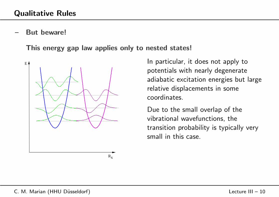
– But beware!

This energy gap law applies only to nested states!

R

E

x

In particular, it does not apply topotentials with nearly degenerateadiabatic excitation energies but largerelative displacements in somecoordinates.

Due to the small overlap of thevibrational wavefunctions, thetransition probability is typically verysmall in this case.

Qualitative Rules


– The strong coupling limit is characterized by large relative displacements insome coordinates so that an intersection of the potential energy surfaces canbe expected.

R

E

x

The probability of the radiationlesstransition exhibits a Gaussiandependence on the energy parameter∆E −EM , where EM is the molecularrearrangement energy for the twoelectronic states under consideration.

Occasionally an inverse relationshipbetween the transition probability and∆E is observed, i.e., there exist caseswhere the probability increases withincreasing energy gap.

General Considerations and Size of ISC Rate Constants


The ISC rate constant depends onthe size of the

– electronic SOC and

– vibrational overlap and on the– density of accepting states

Excited-state ISC rate constants inheteronuclear organic molecules

– Fast 1011 − 1012 s−1

– Typical 108 − 109 s−1

– Slow 105 − 106 s−1

R

E

x R

E

x R

E

x

Ultrafast transitions: ⇒ Nonadiabatic wavepacket dynamics Fast - slow transitions: ⇒ Static approach, Fermi’s Golden Rule

Static Approach: Fermi’s Golden Rule

Calculation ofIntersystem Crossingand ReverseIntersystem CrossingRate Constants

Qualitative Rules

⊲

Static Approach:Fermi’s GoldenRule

Golden Rule

Example

CondonApproximation

Energy Domain

Time Domain

Temperature

Example

Vibronic Effects

Example

Summary

Literature


The Fermi Golden Rule Approximation


Within the Fermi golden rule approximation, the rate k for the irreversibledecay of an initial state |i〉, coupled by a perturbation H(1) to a set of finalstates 〈f |, is given by

k =2π

~

∑

f

|H(1)if |2δ(Ei − Ef ) (79)

The δ distribution ensures the conservation of the molecular energy for thenonradiative transition.

Preconditions for the applicability of the golden rule approximation:

– The interaction of the two states is small compared to their adiabaticenergy difference.

– The density of final vibrational states (VDOS) at the energy of the initialstate is high.

Partitioning of the Molecular Hamiltonian


There are several ways of partitioning the molecular Hamiltonian into azeroth-order Hamiltonian H(0) and a perturbation H(1).

1. HSO is included in the electronic Hamiltonian⇒ Basis states are spin–orbit coupled Born-Oppenheimer states:H(1) is given by the nuclear kinetic energy operator TN.

2. HSO is not included in the electronic Hamiltonian⇒ Basis states are pure-spin Born-Oppenheimer states:H(1) is given by the sum of TN and HSO.The action of TN on the wavefunction may lead to vibronic interactionterms that modulate the ISC process.

Here, we concentrate on the latter approach.

ISC Rate Constants Pure-Spin BO states


In a two-state process, nonadiabatic coupling matrix elements (NACMEs)between the initial and final electronic states of an ISC vanish because of theirdifferent multiplicities.

Up to second order in Rayleigh-Schrodinger perturbation theory, the couplingbetween vibrational state vaj of a singlet state ΨSa and the fine-structurecomponent α of a vibrational level vbk of a triplet state ΨTb

is given by

H(1)aj,bk

α ≈ 〈ΨSa , vaj | HSO |ΨαTb, vbk〉 (80)

+∑

d 6=b

∑

m

〈ΨSa , vaj | HSO |ΨαTd, vdm〉〈Ψα

Td, vdm | TN |Ψα

Tb, vbj〉

Edm − Ebk(81)

+∑

c6=a

∑

l

〈ΨSa , vaj | TN |ΨSc , vcl〉〈ΨSc , vcl | HSO |ΨαTb, vbk〉

Ecl − Ebk(82)

The spin-vibronic interaction terms (81) and (82) are often neglected. Theycan become decisive in TADF emitters with close-lying CT and LE states!

Example: Spin-vibronic interaction in a TADF emitter


1CT and 3CT are nested states, 0.06 eV apart ⇒ weak coupling limit

Direct SOC is tiny, |〈1CT|HSO|3CT〉|2 < 10−3 cm−2 .

O

O

N

ACRXTN

1CT

3ππ∗3nπ∗

3CT

3CT

1CT3ππ∗3nπ∗

C O

(C. M. Marian, J. Phys. Chem. C 120 (2016) 3715.)

Strong nonadiabatic coupling of

– 1nπ∗ and 1CT– 3nπ∗ and 3CT

Decent SOC between

– 1nπ∗ and 3ππ∗

– 3nπ∗ and 3ππ∗

ISC Rates of Pure-Spin Born-Oppenheimer States


If we neglect the spin-vibronic interaction terms (81) and (82), the decay rateof an initially populated ΨSa , vaj vibronic state via ISC to a quasicontinuum offinal vibronic states Ψα

Tb, vbk is given by

kISC =2π

~

∑

α

∑

k

|〈ΨSa , vaj | HSO |ΨαTb, vbk〉|

2 δ(Eaj − Ebk) (83)

Taylor expansion in the vibrational coordinates Q series about an appropriatelychosen reference point q0 yields

〈ΨSa , vaj | HSO |ΨαTb, vbk〉 ≈ 〈ΨSa , | HSO |Ψα

Tb〉∣

∣

∣

q0〈vaj | vbk〉 (84)

+∑

K

∂〈ΨSa | HSO |ΨαTb〉

∂QK

∣

∣

∣

∣

∣

q0

〈vaj |QK | vbk〉 (85)

+ . . .

Condon Approximation


The expansion is usually truncatedat the constant term (84) (“direct spin–orbit coupling”) orat the term (85) linear in QK (“vibronic spin–orbit interaction”).

In the Condon approximation, i.e., assuming only direct SOC, the electronicand vibrational contributions to the ISC rate can be separated.

kFCISC ≈2π

~

∑

α

|〈ΨSa | HSO |ΨαTb〉∣

∣

∣

2

q0

∑

k

|〈vaj | vbk〉|2 δ(Eaj − Ebk) (86)

=2π

~

∑

α


∣

∣

2

q0ρ(Eaj) (87)

where ρ(Eaj) is the VDOS at the energy of the initial state.

Instead of determining the VDOS at the energy of the initial state explicitly, itis more convenient to replace the delta distribution in Eq. (86) by anappropriate expression in the energy or time regimes.

Determining Vibrational Contributions in the Energy Domain


In this approach, the delta function in Eq. (86) is replaced by a step functionof finite width.

In Condon approximation, thevibrational part of the rate isobtained by explicitly summingover the Franck-Condon factors ofall states in the interval η.

kISC =2π

~η

∑

α


∣

∣

2

q0

∑

k | η>|(Eaj−Ebk)|

|〈vaj | vbk〉|2 (88)

The sensitivity of the calculated rate with respect to the interval width η hasto be tested carefully in each case.

The approach is straight forward, but too time-consuming for large moleculesand large energy gaps.

It is not easily extended to include temperature effects (RISC).

Determining Vibrational Contributions in the Time Domain


The time-dependent approach employs a Fourier transform representation ofdelta function in Eq. (86).

δ(Eaj − Ebk) =

∫ +∞

−∞eit(Eaj−Ebk)dt (89)

In the harmonic oscillator model and making use of the Condon approximation,the ISC rate can be determined by numerical integration of

kcorrISC = |〈ΨS |HSO|ΨT 〉|2

∫ ∞

−∞dtG (t) eit(∆E0

ST+ 1

2TrΩS) (90)

where ΩS is a diagonal matrix containing the harmonic frequencies of theinitial state and the correlation function G (t) depends on the normalcoordinates and harmonic frequencies of the initial and final states.

Determining Vibrational Contributions in the Time Domain


To ensure convergence of the time integration, a Gaussian (or Lorentzian)damping function is introduced.

From a physical point of view, thisdamping is consistent with adephasing of the correlationfunction due to the interactionwith a bath (solution) or theredistribution of vibrational energy(gas phase).

The sensitivity of the calculated rate with respect to the width of the dampingfunction has to be tested carefully in each case.

Adding Temperature in the Time Domain


So far, all rates were calculated for vibrationally cold molecules.

For RISC, thermal population of higher vibrational levels is needed.

Assume a Boltzmann population ofvibrational states.

Z =∑

k

e−βEk (91)

is the canonical partition function for vibrational motion in the initial state andβ the inverse temperature.

The rate constant for RISC from a manifold of thermally populated initialvibronic states k then is

kRISC(T ) =2π

Z

∑

j,k

e−βEk |〈ΨSa , vaj | HSO |ΨTb, vbk〉|

2 δ(Eaj − Ebk) (92)

Example: Thermal ISC and RISC in NHC-Copper(I)-Phen Complex


First excited states have mixedMLCT and L′LCT character.

At 298K, ISC is about 100× fasterthan RISC.

2626 2828

Cu 11

N1111

1414

1515 1212

1616

1313

44

77

2020 2222

N2255

66

33

2424

3535

3232

3636 3333

3131

3434IPr

IPr

N2525

N3030

IPr

IPr4242

40404343 4444

4141

4545

Radiative decay via thermally activated delayed fluorescence andphosphorescence can compete.(J. Foller et al., Inorg. Chem. 55 (2016) 7508.)

Beyond the Condon Approximation


When direct SOC is very small, it is often meaningful to include vibronicspin–orbit effects.

In addition to the Condon term (86), two contributions to the ISC rate areobtained from the derivative coupling terms.

1. A cross term that contains Franck-Condon- and Herzberg-Teller-like expressions

kFC/HTISC =

4π

~ℜ

(

〈ΨSa | HSO |ΨTb〉∣

∣

∣

q0

∑

k

〈vaj | vbk〉 δ(Eaj − Ebk)

∑

K

∂〈ΨSa | HSO |ΨTb〉

∂QK

∣

∣

∣

∣

∣

q0

∑

l

〈vaj |QK | vbl〉 δ(Eaj − Ebl)

(93)

Beyond the Condon Approximation


2. A term that stems exclusively from the derivative couplings.

kHTISC =

2π

~ℜ

∑

K


∂QK

∣

∣

∣

∣

∣

q0

∑

k

〈vaj |QK | vbk〉 δ(Eaj − Ebk)

∑

L


∂QL

∣

∣

∣

∣

∣

q0

∑

l

〈vaj |QL | vbl〉 δ(Eaj − Ebl)

(94)Herein ℜ denotes the real part of the expression.

Vibronic interactions can substantially increase the ISC rates, making1(ππ∗) ;

3 (ππ∗) transitions nearly as allowed as 1(ππ∗) ;3 (nπ∗) or

1(nπ∗) ;3 (ππ∗) transitions.

Important mechanism if (nπ∗) states are not accessible for mediating anEl-Sayed-forbidden ISC between a singlet and a triplet (ππ∗) state.

Example: Effect of Aqueous Solution on ISC in Flavin


Apolar solution

– ISC channelS1(ππ

∗) ;T2(nπ∗)

– Direct ISC kISC ≈ 109 s−1

E

3

3

3

1

(ππ∗)

(ππ∗)

(ππ∗)( π∗)

( π∗)

n

n1

ISC

Aqueous solution

– ISC channelS1(ππ

∗) ;T2(ππ∗)

– Vibronic SOC kISC ≈ 108 s−1

3

n

(ππ∗)1

(ππ∗)

E

(ππ∗)3

( π∗)n1

3( π∗)

ISC

Environment changes size and mechanism of ISC!(S. Salzmann et al., J. Photochem. Photobio. A: Chemistry 198 (2008) 221.)

Example: Vibronic SOC and ISC in Porphyrin


All low-lying states are of (ππ∗) type; first (nπ∗) ca. 3 eV above T1

Direct SOC

– S1/T1 SOME≈0.05 cm−1

– S1/T1 kISC ≈ 105 s−1

Vibronic SOC

– Out-of-plane modes mix in(nπ∗) character

– S1/T1 kISC ≈ 107 s−1

(S. Perun et al., ChemPhysChem 9 (2008) 282.)

Summary


Qualitative rules may be used to estimate the size of electronic spin–orbitcoupling between two states.

The energy gap law is applicable only for nested states!

Electronic SOME between 1CT and 3CT is usually very small.

Nonadiabatic interactions with close-by LE states can markedly increase theSOC.

This is also true for symmetry-breaking vibrational discplacements.

Static approaches can be used to compute rate constants for ISC and RISCbetween two states.

If more than two electronic states are involved, dynamic approaches arerequired (but also much more expensive).

Summary


In my view, the most critical ingredients for the computation of ISC and RISCrate constants are the potential energy surfaces.

DFT/MRCI and DFT/MRSOCI appear to do a good job in this respect.

So far, I did not come across a single density functional which yields abalanced description of CT and LE states in organic TADF emitters of thedonor–acceptor type.

Interstate SOMEs can be obtained from TDDFT amplitudes via approximatemany-electron wavefunctions.

SOMEs are much less sensitive to the quality of the wavefunctions thanenergies.

It is in general not suffcient to calculate ISC rate constants for isolatedmolecules. A solvent environment can change probability and mechanism ofISC.

Related Literature


For further details, such as the derivation of equations, and for supplementaryliterature see:

1. Christel M. Marian, Spin–orbit coupling in molecules, Reviews InComputational Chemistry, K. Lipkowitz and D. Boyd, Eds., Wiley VCH,Weinheim, 17 (2001) 99-204

2. Christel M. Marian, Spin–orbit coupling and intersystem crossing in

molecules, Wiley Interdisciplinary Reviews: Computational MolecularScience (2011) 1880-1888; DOI 10.1002/wcms.83

3. Mihajlo Etinski, Vidisha Rai-Constapel, Christel M. Marian,Time-dependent approach to spin-vibronic: Implementation and

assessment, 140 (2014) 114104; DOI 10.1063/1.48684844. Christel M. Marian, Jelena Foller, Martin Kleinschmidt, Mihajlo Etinski,

Intersystem Crossing Processes in TADF Emitters, in: Yersin (Ed.), HighlyEfficient OLEDs, Materials Based on Thermally Activated DelayedFluorescence. Wiley VCH (2018); ISBN: 978-3-527-33900-6

tadf oled krutyn summer school 2017 - excilight · c. m. marian (hhu du¨sseldorf) lecture iii –...

Documents