This article was downloaded by: [University of Oklahoma Libraries]On: 24 August 2014, At: 19:54Publisher: Taylor & FrancisInforma Ltd Registered in England and Wales Registered Number: 1072954 Registered office: Mortimer House,37-41 Mortimer Street, London W1T 3JH, UK

International Journal of Production ResearchPublication details, including instructions for authors and subscription information:http://www.tandfonline.com/loi/tprs20

Tactical production planning in a hybrid Make-to-Stock–Make-to-Order environment under supply,process and demand uncertainties: a robustoptimisation modelMasoud Khakdamana, Kuan Yew Wonga, Bahareh Zohooria, Manoj Kumar Tiwarib & RicoMerkertc

a Department of Manufacturing and Industrial Engineering, Faculty of MechanicalEngineering, Universiti Teknologi Malaysia, Skudai, Malaysiab Department of Industrial Engineering and Management, Indian Institute of Technology,Kharagpur, Indiac Institute of Transport and Logistics Studies, The University of Sydney, Sydney, AustraliaPublished online: 16 Jul 2014.

To cite this article: Masoud Khakdaman, Kuan Yew Wong, Bahareh Zohoori, Manoj Kumar Tiwari & Rico Merkert(2014): Tactical production planning in a hybrid Make-to-Stock–Make-to-Order environment under supply, processand demand uncertainties: a robust optimisation model, International Journal of Production Research, DOI:10.1080/00207543.2014.935828

To link to this article: http://dx.doi.org/10.1080/00207543.2014.935828

PLEASE SCROLL DOWN FOR ARTICLE

Taylor & Francis makes every effort to ensure the accuracy of all the information (the “Content”) containedin the publications on our platform. However, Taylor & Francis, our agents, and our licensors make norepresentations or warranties whatsoever as to the accuracy, completeness, or suitability for any purpose of theContent. Any opinions and views expressed in this publication are the opinions and views of the authors, andare not the views of or endorsed by Taylor & Francis. The accuracy of the Content should not be relied upon andshould be independently verified with primary sources of information. Taylor and Francis shall not be liable forany losses, actions, claims, proceedings, demands, costs, expenses, damages, and other liabilities whatsoeveror howsoever caused arising directly or indirectly in connection with, in relation to or arising out of the use ofthe Content.

This article may be used for research, teaching, and private study purposes. Any substantial or systematicreproduction, redistribution, reselling, loan, sub-licensing, systematic supply, or distribution in anyform to anyone is expressly forbidden. Terms & Conditions of access and use can be found at http://www.tandfonline.com/page/terms-and-conditions

Tactical production planning in a hybrid Make-to-Stock–Make-to-Order environment undersupply, process and demand uncertainties: a robust optimisation model

Masoud Khakdamana, Kuan Yew Wonga*, Bahareh Zohooria, Manoj Kumar Tiwarib and Rico Merkertc

aDepartment of Manufacturing and Industrial Engineering, Faculty of Mechanical Engineering, Universiti Teknologi Malaysia,Skudai, Malaysia; bDepartment of Industrial Engineering and Management, Indian Institute of Technology, Kharagpur, India;

cInstitute of Transport and Logistics Studies, The University of Sydney, Sydney, Australia

(Received 23 July 2013; accepted 11 June 2014)

In this paper, we consider a hybrid ‘Make-to-Stock–Make-to-Order’ environment to develop a novel optimisation modelfor medium-term production planning of a typical multi-product firm based on the competencies of the robust optimisationmethodology. Three types of uncertainties: suppliers, processes and customers, are incorporated into the model to constructa robust practical model in an uncertain business environment. The modelling procedure is started with applying determin-istic linear programming to develop a new multi-objective approach for the combination of multi-product multi-periodproduction planning and aggregate production planning problems. Then, the proposed deterministic model is transformedinto a robust optimisation framework and the solution procedure is designed according to the Lp-Metric methodology.Next, using the IBM ILOG CPLEX optimisation software, the proposed model is evaluated by applying the data collectedfrom an industrial case study. Final results illustrate the applicability of the proposed model.

Keywords: Make-to-Stock; Make-to-Order; multi-product multi-period production planning; aggregate productionplanning; robust optimisation; uncertainty

1. Introduction

Creating shareholder value is commonly considered as the principal business goal. To achieve a global and integratedsystem, strategic decisions should be taken in close relation to the more tactical issues (Goetschalckx, Vidal, and Dogan2002). Traditionally, pure Make-to-Stock (MTS) or pure Make-to-Order (MTO) production strategies are applied inmanufacturing firms; however, nowadays, many companies benefit from the combination of both MTS and MTO strate-gies to have better resource utilisation, customer satisfaction and market share.

To date, many studies in the area of production planning have been performed using a variety of approaches which canbe categorised into analytical (Wang and Fang 2001; Sodhi and Tang 2009), artificial intelligence (Tavakkoli-Moghaddamet al. 2007; Zhu and Zhang 2009), simulation (Genin, Thomas, and Lamouri 2007) and hybrid (Kallrath 2005; Jamalniaand Soukhakian 2009) approaches. In addition, demand, process and supply can be considered as the three main types ofuncertainties (Dai, Fan, and Sun 2003; Kazemi Zanjani, Nourelfath, and Ait-Kadi 2010) which will make any medium-term plan obsolete, thus forcing a re-planning cycle. Here, the main question is how to construct a robust plan whichremains valid for a longer time and insensitive to the effects of uncertainties. Reviewing the current literature illustratesthat many studies have been conducted on controlling and reducing the impact of uncertainties on medium-term productionplanning; however, research in the area of tactical production planning for firms applying the hybrid MTS–MTO strategyis still in the infant stages. Here, combined MTS–MTO environments require the development of robust tactical plansunder uncertain situations. Thus, this research takes a multi-product, multi-period and multi-objective environment intoaccount to develop a robust tactical plan for the hybrid MTS–MTO manufacturing system under demand, process and sup-ply uncertainties. This is achieved through the development of a novel multi-objective mathematical model that integratesboth push and pull systems simultaneously, and the application of the robust optimisation methodology.

In the remainder of the paper, the following sections are discussed. Sections 2 and 3 provide a comprehensive litera-ture review and the research methodology, respectively. Section 4 shows the proposed approach which is evaluatedusing an industrial case study in Section 5. Results and discussion are demonstrated in Section 6. Final conclusions andfuture research directions are provided in Section 7.

*Corresponding author. Email: wongky@mail.fkm.utm.my

© 2014 Taylor & Francis

International Journal of Production Research, 2014http://dx.doi.org/10.1080/00207543.2014.935828

Dow

nloa

ded

by [

Uni

vers

ity o

f O

klah

oma

Lib

rari

es]

at 1

9:54

24

Aug

ust 2

014

2. Literature review

2.1 Multi-product multi-period and aggregate production planning problems under uncertainty

Two types of tactical production planning problems are the multi-product multi-period (MPMP) production planningand the aggregate production planning (APP) problems. The former attempts to determine the production quantities ofdifferent products to be matched with the market demand over a planning horizon. The latter aims at satisfyingcustomers’ demands over a medium-term planning horizon by determining the optimal levels of inventory, workforce,backorder, subcontracting and overtime production.

As explained by Hax and Candea (1984) and Billington, McClain, and Thomas (1983), the standard form of theMPMP model considers the minimisation of the total production-related costs (variable production, inventory and short-age costs) as the objective function. Akif Bakir and Byrne (1998) presented a stochastic linear programming model inwhich the feasibility of the solution is affected by uncertain demands. Since then different stochastic programmingapproaches have been adopted (e.g. Kazaz, Dada, and Moskowitz 2005; Kazemi Zanjani, Nourelfath, and Ait-Kadi2010). Then, Byrne and Bakir (1999) demonstrated a hybrid analytical-simulation approach in an industrial manufactur-ing firm for coping with complex behaviours of resource consumption. Application of hybrid approaches can also befound in Thompson and Davis (1990) (analytical-simulation), Dai, Fan, and Sun (2003) (fuzzy linear programming-freezing parameter simulation), Garcia-Sabater, Maheut, and Garcia-Sabater (2009) (decision support system-mixed inte-ger linear programming), etc. Wang and Fang (2001) proposed a multi-objective fuzzy linear programming approach tocope with several uncertainties in an APP problem which covers overtime, backlogging and subcontracting and aims tomaximise profit and minimise workforce change simultaneously. In this regard, artificial intelligence methodologies havebeen vastly applied (see for instance Wang and Liang 2005 (fuzzy linear programming), Jamalnia and Soukhakian 2009(fuzzy non-linear programming and genetic algorithm), and Liang et al. 2011 (fuzzy linear programming)).

One of the first applications of robust optimisation in production planning is presented by Leung and Wu (2004).They applied a robust non-linear optimisation model to minimise the total costs of a typical APP problem with over-time, shortage cost and subcontracting variables, while backorder is not allowed. They also incorporated uncertaintieslike market demand, sales price, shortage cost, inventory cost, human resource costs (hiring and layoff), production costand subcontracting cost into their problem. Leung et al. (2007) presented a robust linear optimisation approach toaddress a multi-site APP problem in the presence of uncertainties such as demand, shortage cost, inventory cost, produc-tion cost and human resource cost. Sitompul and Aghezzaf (2008) evaluated the performance of two robust planningmodels for a multi-period APP problem in the presence of demand fluctuations and concluded that the alternative modelhas more stability and less computation time while the scenario-based model has more flexibility. Kazemi Zanjani,Ait-Kadi, and Nourelfath (2010) applied the robust optimisation approach to maximise the customer service level oftheir proposed model, while Aghezzaf, Sitompul, and Najid (2010) presented three mixed approaches. Considering amulti-product, multi-period and multi-site environment, Al-e-Hashem, Malekly, and Aryanezhad (2011) solved an APPproblem under several uncertainties by using a novel robust mixed integer non-linear programming approach aimed tosatisfy both objectives of minimising total costs and maximising customers’ satisfaction. Moreover, Al-e-Hashem,Aryanezhad, and Sadjadi (2012) extended their study using a hybrid approach (robust optimisation and geneticalgorithm) and adding the maximisation of the workers’ productivity as a new objective function.

2.2 MTS–MTO hybrid environment

In contrast to the MPMP and APP problems, there are only a handful of studies on production planning and control ofthe MTS–MTO environment demonstrating that research in this area is still in infant stages. Williams (1984) conductedone of the first studies on the MTS–MTO hybrid production environment in which some issues like the selectionmethod of MTS or MTO strategy, batch size for MTS, amount of inventory for products selected as MTS and availabil-ity ratio for products chosen as MTO, are discussed. Bemelmans (1986) explained the concept of capacity-orientedinventory-uncertainty for the demand of a typical product and discussed that it can be covered through the stock ofanother product with more or less uncertain demand. Carr et al. (1993) used a M/D/1 queue for modelling theMTS–MTO system and indicated that their proposed model needs less cost than the pure MTS strategy. Likewise,Nguyen (1998) depicted the combined MTS–MTO system as a mixed queuing network. Mu (2001) presented a mathe-matical model to design a combined MTS–MTO environment aimed to find the appropriate economical base stock leveland location for satisfying the specified service constraint. Unlike Williams (1984), Rajagopalan (2002) allowed lowdemand items to follow the MTS strategy and provided a heuristic procedure to solve a non-linear integer programmingformulation that determines the MTS–MTO partition. Soman, van Donk, and Gaalman (2004) demonstrated a holistichierarchical production planning framework for production management decisions. Zaerpour et al. (2008) developed a

2 M. Khakdaman et al.

Dow

nloa

ded

by [

Uni

vers

ity o

f O

klah

oma

Lib

rari

es]

at 1

9:54

24

Aug

ust 2

014

hybrid fuzzy Analytic Hierarchy Process – Strengths, Weaknesses, Opportunities and Threats methodology for theMTS–MTO system to depict a strategic decision-making approach for partitioning products. Finally, Rafiei and Rabbani(2011) presented a model for determining which products should be produced based on the MTS, MTO and combinedMTS–MTO strategies.

Having analysed the above papers, key weaknesses of the previous literature can be summarised as follows:

� Lack of consideration of multi-objective approaches which does not portray today’s business environment asrealistic as possible because organisations have multiple objectives or goals, rather than just a single one.

� Lack of consideration of multi-product environments which is not fully applicable in practice as organisationsproduce multiple products for various customers.

� Building a model in a single-uncertainty environment is not realistic as only demand is often considered as anuncertain parameter, while other sources of uncertainty such as process and supply are ignored.

� Previously developed models have not covered all components of a standard APP problem (Chopra and Meindl2010) and as a result, they do not yield a complete and comprehensive production plan.

� As highlighted by Gupta and Maranas (2003), developing a model in the pure MTS or pure MTO environmentmasks the challenges of today’s competitive business environment (for example, most of the studies inSection 2.1). What is required is a combination of MTS and MTO strategies rather than one of them per se.

As illustrated above, most of the previous models are over-simplified, not realistic and less applicable to deal withthe true nature of current business situations. To the best of the authors’ knowledge, no research exists in the currentliterature to construct a robust tactical production planning model for combined MTS–MTO strategies.

2.3 The need for robust optimisation

Since the applicability of the model in real-world circumstances is very important, a suitable method capable of han-dling uncertainties should be selected. In addition, the method should be able to cope with the simultaneous integratedplanning of MTS and MTO products to achieve the maximum resource utilisation which is one of the principal aims ofcompanies applying the MTS–MTO business strategy. In order to address these two issues, the robust optimisationapproach is used in this research as opposed to other techniques such as fuzzy logic and stochastic programming.

Fuzzy logic has certain disadvantages despite it being beneficial for considering uncertainties. When the complexityof a system increases, the determination of a correct and accurate set of rules becomes more difficult and challenging,and a substantial amount of time is needed to adjust the rules in order to obtain good solutions. Another issue isdefuzzifying a suitable and feasible solution that can operate in all prospective conditions may be impossible. Stochasticprogramming requires a deep knowledge of the probability distribution of the uncertainty. Furthermore, its solutions aredifficult to understand (Powell and Topaloglu 2003). The main distinction between stochastic programming and robustoptimisation is that the former optimises only the first moment of the distribution of the objective function. In fact, itignores higher moments of the distribution which are especially important for asymmetric distributions, and neglects thepreferences of decision-makers towards risk which are critical for risk-averse decision-makers. Moreover, focusing onexpected value optimisation in stochastic programming requires an active management style (high interventions fromdecision-makers) since the expected value can still remain optimal even though when large changes in the objectivefunction are observed.

Conversely, in robust optimisation, the control variables are easily adjusted as scenarios unfold. However, since thevalue of the objective function will not differ significantly among different scenarios, little or no adjustment of the con-trol variables is needed. Thus, robust optimisation enables (compared to all other methods) a more passive managementstyle by minimising higher moments of the objective function (for example, the variance of the objective function’s dis-tribution). Another advantage is the handling of the constraints. Stochastic models intend to find a design variable’svalue so that for each scenario, a possible control variable’s setting satisfies the constraints. Here, when no feasible pairof design and control variables is possible for every scenario, a stochastic programming model is declared as infeasible.Robust optimisation explicitly allows this possibility which is a common observation in engineering applications(Mulvey, Vanderbei, and Zenios 1995).

2.4 Robust optimisation methodology

Mulvey, Vanderbei, and Zenios (1995) introduced the robust optimisation methodology as a proactive approach to math-ematical programming in which the goal programming approach is combined with a set of scenarios as input data toproduce less sensitive solutions to noisy data from scenarios. Decision variables in robust optimisation are design andcontrol variables. The optimal values of design variables are not impacted by uncertain parameters; however, control

International Journal of Production Research 3

Dow

nloa

ded

by [

Uni

vers

ity o

f O

klah

oma

Lib

rari

es]

at 1

9:54

24

Aug

ust 2

014

variables are adjusted once an uncertain parameter is observed. In addition, two types of constraints which are structuralconstraints without noisy coefficients, and control constraints with noisy coefficients are applied. Assume that x 2 Rn1 isthe design variables vector and y 2 Rn2 is the control variables vector. Then the basic linear programming model isformed as follows:

Min cTxþ dTy x 2 Rn1; y 2 Rn2 (1)

Subject to: Ax ¼ b (2)

Bxþ Cy ¼ e (3)

x; y > 0 (4)

Equation (2) is the structural constraint with fixed coefficients, whilst Equation (3) shows the control constraintaffected by noisy coefficients. Equation (4) guarantees non-negative vectors. In the robust formulation, a set of scenariosX ¼ f1; 2; 3. . .Sg is defined where under each scenario s 2 X , the control constraints’ coefficients (d, B, C and e) willbecome fds;Bs;Cs; esg with a predetermined probability qs, the occurrence probability of scenario s, thus,

PSs¼1qs ¼ 1.

In terms of optimality, the optimal solution of the robust model is called ‘robust solution’ when it remains ‘close’ tooptimality for any realisation of scenario s. However, in terms of feasibility, the model is called ‘robust model’ if itremains ‘almost’ feasible for any realisation of scenario s. It is not possible to find solutions which remain both feasibleand optimal for all of the scenarios. For this reason, robust optimisation measures the trade-off between model robust-ness and solution robustness by applying the concept of multi-criteria decision-making (MCDM) as follows.

For each scenario, firstly, the vector of control variables ys is introduced and then the error vector ds is defined tomeasure the allowed infeasibility of control constraints. Secondly, the basic linear programming model (Equations(1)–(4)) is transformed into the following robust model.

Min r x; y1; . . .; ysð Þ þ xqðd1; . . .; dsÞ (5)

Subject to: Ax ¼ b (6)

Bsxþ Csyþ ds ¼ es 8s 2 X (7)

x� 0; ys � 0 8s 2 X (8)

It is considerable that by realisation of each scenario, the single choice for an aggregate objective in Equation (1),n ¼ cTxþ dTy, becomes a random variable which takes the value ns ¼ cTxþ dTs ys with the occurrence probability ofqs. Here, robust optimisation applies the expected value of all ns by utilising the stochastic function rð�Þ ¼Ps2Xqsns.In this regard, robust optimisation could be considered as a stochastic non-linear programming model, since it allowshigher moments of the distribution of ns in the optimisation model. However, Mulvey, Vanderbei, and Zenios (1995)discussed that using just the stochastic function

Ps2Xqsns is not capable of coping with moderate to high risk decisions

under uncertainty. Therefore, they suggested that a suitable choice for rð�Þ would be the mean plus a constant k timesthe variance (Equation (9)). By considering the variance as a representative for risk, it is obvious that a high variancefor ns means that the outcome is much in doubt. Thus, the expected outcome should be minimised for a given risk level(Equation (9)). In this respect, k is a weighting factor to trade-off between risk and expected outcome for the solutionrobustness. Hence, as k increases in Equation (9), the problem is led to the solutions which are less sensitive to changesin the data defined by the scenarios.

r x; y1; . . .; ysð Þ ¼Xs2X

qsns þ kXs2X

qs ns �Xs02X

qs0ns0

!2

(9)

Investigating Equation (9), it is obvious that it contains a quadratic termP

s2Xqsðns �P

s02Xqs0ns0 Þ2 which makesthe formulation non-linear and complex. In addition, Yu and Li (2000) demonstrated that the minimisation of thisobjective (Equation (9)) consumes a great deal of computation. Therefore, they suggested the following formulation(Equation (10)) which is simpler; however, Wagner (1975) introduced two non-negative deviational variables totransform the problem into a linear programming model. In this procedure, instead of minimising the sum of absolutedeviations in Equation (10), two deviational variables will be minimised, subjected to the original constraints andadditional soft constraints which give positive values of the difference inside the absolute functions.

4 M. Khakdaman et al.

Dow

nloa

ded

by [

Uni

vers

ity o

f O

klah

oma

Lib

rari

es]

at 1

9:54

24

Aug

ust 2

014

r x; y1; . . .; ysð Þ ¼Xs2X

qsns þ kXs2X

qs ns �Xs02X

qs0ns0

���������� (10)

However, Yu and Li (2000) discussed that performing this direct linearisation requires many non-negative deviationalconstraints and variables and is therefore largely restricted. Finally, Yu and Li (2000) proposed an efficient methodologywhich is depicted in Equations (11)–(13) where hs shows the deviation for violation of the mean.

Min Z ¼Xs2X

qsns þ kXs2X

qs ns �Xs02X

qs0ns0

!þ 2hs

" #(11)

ns �Xs02X

qs0ns0

!þ hs � 0 (12)

hs > 0 (13)

In Equation (11), it is notable that if ns �P

s02Xqs0ns0 � 0, then hs ¼ 0 and Z ¼Ps2X qsnsþkP

s2X qs½ns �P

s02X qs0ns0 �. In contrast, if ns �P

s02X qs0ns0 � 0, then hs ¼P

s02X qs0ns0 � ns andZ ¼Ps2X qsns þ k

Ps2X qs½

Ps02X qs0ns0 � ns�. As can be seen, the solution procedure of Equations (11)–(13) is the

same with Equation (10).The second term in the objective function (Equation (5)), q d1; . . .; dsð Þ, is named as a infeasibility penalty function

which is applied for some of the scenarios to penalise violations of the control constraints. In other words, this penaltyfunction is used to punish infeasible solutions created by some of the scenarios. Finally, the formulation of the robustobjective function which includes both solution robustness and feasibility robustness is as follows.

Min Z ¼Xs2X

qsns þ kXs2X

qs ns �Xs02X

qs0ns0

!þ 2hs

" #þ x

Xs2X

qsds (14)

Here, by employing the goal programming weight x, a MCDM process could be applied to trade-off solutionrobustness versus model robustness. For example, when x ¼ 0, the objective would be minimising the term r �ð Þ whichmay lead the problem to an infeasible solution; while if an adequately large value is allocated to x, the term q �ð Þ willdominate the objective function, resulting in higher costs.

3. Research methodology

In this research, we applied a stepwise approach and each step is discussed as follows:

(1) The notions of the standard MPMP problem are combined with constraints and objectives of the APP problemto develop a novel deterministic multi-objective linear programming model in a typical MTS–MTO environ-ment. Here, developing a new mathematical model for tactical production planning in a MTS–MTO environ-ment signifies the main contribution of this research.

(2) In order to examine the efficiency of the proposed deterministic model, it is solved using case study datathrough the IBM ILOG CPLEX optimisation software and the optimal solution is obtained.

(3) Since we aim to develop the model for real-world situations where different types of uncertainties and risksexist, the next step is to identify and incorporate demand, supply and process uncertainties into the proposeddeterministic model by transforming it into a robust optimisation framework.

(4) The proposed robust model is solved twice (using IBM ILOG CPLEX), each time with one of the objectivefunctions (cost and efficiency).

(5) Both optimal objective functions are applied to solve the proposed final robust model (multi-objective) byutilising the Lp-Metric methodology (using one set of weighting factors (ui)) to obtain the optimum solution.

(6) Finally, different levels of weighting factors (ui) are considered to indicate the impact of a decision-maker’sopinion on the importance of each objective function for the proposed final robust model.

Since the Lp-Metric methodology is applied in this study, a more comprehensive explanation of this weighted metricmethod is provided here. Basically, it belongs to the category of multi-objective decision-making (MODM) methods thataggregate multiple objective functions into one dimension and where a decision-maker provides the required information

International Journal of Production Research 5

Dow

nloa

ded

by [

Uni

vers

ity o

f O

klah

oma

Lib

rari

es]

at 1

9:54

24

Aug

ust 2

014

before solving the problem (Aryanezhad et al. 2009). We use this approach as it requires only little information fromdecision-makers, it is easy to implement in practical situations, and it provides a flexible tool for decision-makers toincorporate their desires into the decision-making process.

To explain the Lp-Metric method, if Z�i shows the optimum solution value when the model is solved with only one

objective function, then ZLp�Metric (Equation (15)) shows the integrated objective function, where ui is a weightingfactor indicating the importance of the ith objective function determined by decision-makers.

Min ZLp�Metric ¼Xi

uiððZi � Z�i Þ=Z�

i Þ (15)

Xi

ui ¼ 1 (16)

0�ui � 1 (17)

As an illustration, assume that a MODM problem has three objectives of minimising total cost (Z�1 ), maximising

customer satisfaction (Z�2 ) and maximising production utilisation (Z�

3 ). Assume that the importance of each of the aboveobjective functions for the decision-maker (i.e. manager) are u1 (e.g. 0.5), u2 (e.g. 0.3) and u3 (e.g. 0.2), respectively.Thus, we would have the following equation for finding the optimal solution:

Min ZLp�Metric ¼ 0:5Z1 � Z�

1

Z�1

þ 0:3Z2 � Z�

2

Z�2

þ 0:2Z3 � Z�

3

Z�3

(15 Continued)

4. Model formulation

4.1 Proposed model

This section details our model which is constructed based on the combination of MPMP production planning problemswith APP problems. The proposed model is developed for companies which benefit from both strategies of MTS andMTO simultaneously. The products are categorised into two groups. The first category belongs to ‘MTS products’ whichare produced based on the MTS business strategy that forecasts the demand as well as the required materials and com-ponents based on historical data and experience, and plans a routine production to provide products to the market. Thesecond category of products is derived from the MTO business strategy and named here ‘MTO products’. For MTOproducts, companies have a forecasting scheme to predict the required raw materials and components, while theypostpone certain production processes until they receive the customers’ order. To be more efficient and responsive, theyperform some general processes of some products for better utilisation of their resources.

In fact, the main difference between MTS and MTO strategies is their production postponement point. MTS is apure speculation mode without postponing any of the production processes (e.g. fabrication, assembly and packaging) tothe time of receiving an actual order. In contrast, there is a unique postponement point for MTO products. For example,some companies postpone their fabrication and assembly processes, while some organisations start their fabrication pro-cess beforehand and postpone their assembly activity. In certain industries, only the packaging process is postponedwhere both fabrication and assembly are completed beforehand. Production planning can be performed based on themanufacturing of both MTS and MTO products at the same time. The only difference is that the production of MTOproducts is stopped at one of the processes (postponement point) until the actual order is received, and then theremaining processes will be executed. The proposed model is capable of considering both MTS and MTO strategiessimultaneously in a single formulation by taking into account the postponement point.

4.1.1 Proposed deterministic model

4.1.1.1 Model assumptions.

(1) Overtime and subcontracting are allowed for all products. No shortage is allowed for MTS products whilethey could be backordered; for MTO products, neither backorder nor shortage is allowed.

(2) Assuming that suppliers forward raw materials to the manufacturing plant, transportation cost of rawmaterials is endured by suppliers and hence, is not incorporated into the model.

(3) No inventory of raw materials is assumed at the beginning of the planning horizon.

6 M. Khakdaman et al.

Dow

nloa

ded

by [

Uni

vers

ity o

f O

klah

oma

Lib

rari

es]

at 1

9:54

24

Aug

ust 2

014

(4) The lead time for fulfilling the customers’ demand of products is not greater than one planning time period.(5) Inventories of MTO-finished products are not considered in the model since they are sent to the customers

as soon as their production is finished. In addition, work in progress (WIP) inventory is allowed only for thegeneral processes of MTO products.

(6) To develop a more practical production plan, the impacts of poor quality materials, methods, workers,machines and decisions are incorporated into the model by considering quality targets of the company in theproduction plan. In this regard, a parameter bit is defined to indicate the desired quality level of productionwhich is determined by the company’s top managers to achieve the corporate quality goals. It is obvious thatif the company has zero defect processes producing no scrap, the parameter bit ¼ 1:

(7) It is assumed that all of the hired workers need some training to start work. Training cost of hired workers istherefore added to the hiring cost.

(8) Cost-related uncertainties and risks are considered as the most important risks which are capable of affectingthe outcome of planning activities remarkably. Based on this, model uncertainties of this research are catego-rised into the three sides of a typical supply chain including supplier (raw material cost and exchange rate),manufacturer (production cost, backorder cost, inventory holding cost, workforce-related cost, subcontractingcost and transportation cost) and customer (demand). Hence, the rest of the model parameters are assumed tobe fixed.

(9) Constraints related to machine set-up belong to the operational production planning level, and thus they arenot considered in the model which is developed for the tactical production planning level. By definition, tac-tical (aggregate) production planning is mainly concerned with medium-term (3–18 months) decisions on thenumber of required products to fulfil customer demands rather than short-term issues on operational produc-tion planning such as machine set-up (Chopra and Meindl 2010). In reality, machine set-up is normally notconsidered in a company’s medium-term planning because its impact is negligible.

(10) Likewise, the failures of machines and their reliability parameters are not incorporated into the modelbecause they are assumed to be addressed in the operational production planning level. In essence, issuessuch as set-up, failure and other disruptions should be taken care in the operational level, which will thenbecome the inputs for the tactical level.

4.1.1.2 Mathematical formulation.� Index sets

i Products, i = 1,2,…,ib,…,izj Processes, j = 1,2,…,jb,…,jzm Machine centres, m = 1,2,…,Mk Workers’ skill levels, k = 1,2,…,Kr Raw material types, r = 1,2,…,Ra Inventory types, a ¼ 1 (Raw material), 2 (WIP), 3 (Finished product)g Production time, g ¼ 1 (Regular time), 2 (Overtime)n Customers, n ¼ 1 (Local), 2; . . .;N (International countries)u Suppliers, u ¼ 1 (Local), 2; . . .;U (International countries)c Transportation modes, c ¼ 1 (Road), 2 (Rail), 3 (Air), 4 (Water)t Planning periods, t = 1,2,…,Tib The last MTS product. Products from ib þ 1 to iz are considered as MTO productsjb The process in which the production procedure is stopped waiting for customers’ order and will continue

after confirming the order (this is the postponement point for MTO products only)

� Decision variables

Pijgkt Production quantity of jth process of product i during production time g by worker k in period t (unit)Iijt Inventory quantity of jth process of product i at the end of period t (unit)IRrt Inventory quantity of raw material r at the end of period t (unit)RSrut Quantity of raw material r supplied by supplier u in period t (unit)SQijt Subcontracting quantity of jth process of product i in period t for use in the same period (unit)

International Journal of Production Research 7

Dow

nloa

ded

by [

Uni

vers

ity o

f O

klah

oma

Lib

rari

es]

at 1

9:54

24

Aug

ust 2

014

Bint Quantity of finished product i ordered in period t by customer n which will be backordered for fulfilmentin future periods (unit)

Qinct Quantity of finished product i allocated for customer n by transportation mode c in period t (unit)Hkt Amount of k-type workers hired in period t (man-hour)Fkt Amount of k-type workers laid off in period t (man-hour)

� Parameters

Dint Demand of product i in customer zone n in period t (unit)EXut Exchange rate between suppliers (u) and the manufacturer (local country) which shows the value of one

unit of the supplier country currency against local currency in period tPCijt Production cost (set-up, maintenance, overhead, etc.) of jth process of product i in period t ($/unit)SCijt Subcontracting cost of jth process of product i in period t ($/unit)RCrut Cost of raw material r (in terms of the currency of supplier country) procured from supplier u in period t

($/unit)ICijt Inventory holding cost of product i that completed its jth process in period t ($/unit)IRCrt Inventory holding cost of raw material r in period t ($/unit)BCint Backorder cost of product i for customer n in period t ($/unit)LCkgt Labour cost of k-type workers in production time g in period t ($/man-hour)HtCkt Hiring (and training) cost of k-type workers in period t ($/man-hour)FCkt Firing cost of k-type workers in period t ($/man-hour)TCnct Average transportation cost of sending finished products to customer n by transportation mode c in

period t ($/unit)McMaxmgt Maximum capacity of machine centre m in production time g in period t (machine-hour)IMaxat Maximum available space for inventory type a in period t (m2)PcMaxkgt Maximum available man-hour for production by k-type workers in production time g in period t (man-hour)SMaxijt Maximum available subcontracting volume of jth process of product i in period t (unit)RMaxrut Maximum available quantity of raw material r that could be supplied by supplier u in period t (unit)BMaxint Maximum allowed backorder quantity for product i for customer n in period t (unit)ct Fraction of workforce variation allowed in period t (0\ct\1)bit Desired quality level (target) for production of quality product i in period t (0\bit\1) ((1� bitÞ is

considered as the level of poor quality production)akt Productivity of k-type workers in period t (0\akt\1)MTijkm Processing time of jth process of product i on machine m by worker k (machine-hour/unit)LTijk Labour usage for performing jth process of product i by worker k (man-hour/unit)RUijr Amount of raw material r required for jth process of product i (unit)WRr Warehouse space needed for raw material r (m2/unit)Wij Warehouse space needed for semi-finished and finished product i that completed its jth process (m2/unit)

� Objective function

A multi-objective function is developed to minimise the total costs and maximise the total machines efficiency. The firstobjective function (Equation (18)) is to minimise a firm’s total costs (Z1) by summation of all cost drivers including rawmaterial cost, production cost, workforce cost, inventory holding cost, subcontracting cost, transportation cost and backor-der cost. The second objective function (Equation (19)) aims to maximise the total efficiency of machines (Z2) by consider-ing the fraction of time in which available machines have produced qualified products among all production outcomes.

Min total costs ¼ Min Z1¼Xr;u;t

EXutRCrutRSrut

!þ

Xi;j;g;k;t

PijgktPCijt

!þ

Xi;j;t

SQijtSCijt

!

þXi;j;g;k;t

PijgktLTijkLCkgt þXk;t

ðHktHtCkt þ FktFCktÞ !

þXi;j;t

IijtICijt þXr;t

IRrtIRCrt

!

þXi;n;c;t

QinctTCnct

!þ

Xibi;n;t

BintBCint

!(18)

8 M. Khakdaman et al.

Dow

nloa

ded

by [

Uni

vers

ity o

f O

klah

oma

Lib

rari

es]

at 1

9:54

24

Aug

ust 2

014

Max machines efficiency ¼ Max Z2 ¼X

i;j;k;g;m;t

bitPijgktMTijkm=Xm;g;t

McMaxmgt

!(19)

� Constraints

Equation (20) ensures that inventory of raw materials in each period is equal to those from the previous period plusthe amount supplied in the current period excluding the amount applied for production in the current period. Equation(21) maintains the material balance between periods for MTS products. It shows that the amount of qualified products,subcontracting parts and previous period inventory of each process excluding the quantity stored for future periodsshould be equal to the inventory, subcontracting and production quantities of the next process. In the same manner,Equation (22) is applied for the material balance of processes of MTO products which can be completed before receiv-ing the customers’ order. For the remaining processes of MTO products, however, no inventory is considered fromprevious periods or for future periods (Equation (23)).

In order to satisfy customers’ demand for MTS products in each period, the amount of finished products allocatedfor different customers plus backorders for the next period should be equal to the current demand and previous backor-ders (Equation (24)); while no backorder is allowed for MTO products (Equation (25)). Equation (26) is defined tomake sure that all of the produced, stored and subcontracted finished products of MTS products will be sent to the cus-tomers and surplus of finished products should be stored for future periods; however, inventory of finished MTO prod-ucts is not allowed (Equation (27)). Equation (28) is developed to make sure that the total machine-hour utilisation doesnot exceed the maximum available capacity of the machines. To prevent the amount of subcontracting parts to be morethan the available outsourcing capacity in each period, Equation (29) is applied. Equation (30) is made to consider themaximum amount of raw materials which could be supplied by each supplier in each period. Equation (31) satisfies theconstraint of the maximum capacity of backorder planning for MTS products in each period. Equation (32) is used toensure that the total production time in regular time and overtime would not exceed the maximum productive availableman-hour in each period. Equation (33) maintains the balance between the total available man-hour in each period withthose from previous periods plus the amount of hired workers minus fired labours. In addition, the total workforcechange in each period should not go above the permitted fraction (ct) allowed by firms’ managers or labour unions(Equation (34)). The maximum inventory space for raw materials is shown in Equation (35). Likewise, the maximumWIP inventory space constraint (Equation (36)) is developed by adding inventory space of semi-finished MTS productsto those from MTO ones. Equation (37) indicates the constraint of available space for finished MTS products. Equation(38) ensures that all of the decision variables are non-negative.

IRrt ¼ IRr;t�1 þXu

RSrut �Xi;j;g;k

PijgktRUijr 8r; 8t (20)

bitXg;k

Pijgkt þ SQijt þ Iij;t�1 � Iijt ¼ bitXg;k

Pi;jþ1;gkt þ SQi;jþ1;t þ Ii;jþ1;t�1 8i� ib; 8j� jz � 1; 8t (21)

bitXg;k

Pijgkt þ SQijt þ Iij;t�1 � Iijt ¼ bitXg;k

Pi;jþ1;gkt þ SQi;jþ1;t þ Ii;jþ1;t�1 8ib þ 1� i� iz; 8j\jb; 8t (22)

bitXg;k

Pijgkt þ SQijt ¼ bitXg;k

Pi;jþ1;gkt þ SQi;jþ1;t 8ib þ 1� i� iz; 8jb � j� jz � 1; 8t (23)

Dint þ Bin;t�1 ¼Xc

Qinct þ Bint 8i� ib; 8n; 8t (24)

Dint ¼Xc

Qinct 8ib þ 1� i� iz; 8n; 8t (25)

International Journal of Production Research 9

Dow

nloa

ded

by [

Uni

vers

ity o

f O

klah

oma

Lib

rari

es]

at 1

9:54

24

Aug

ust 2

014

bitXg;k

Pijzgkt þ SQijzt þ Iijz;t�1 � Iijzt ¼Xn;c

Qinct 8i� ib; 8t (26)

bitXg;k

Pijzgkt þ SQijzt ¼Xn;c

Qinct 8ib þ 1� i� iz; 8t (27)

Xi;j;k

PijgktMTijkm �McMaxmgt 8m; 8g; 8t (28)

SQijt � SMaxijt 8i; 8j; 8t (29)

RSrut �RMaxrut 8r; 8u; 8t (30)

Bint �BMaxint 8i� ib; 8n; 8t (31)

Xi;j

PijgktLTijk � aktPcMaxkgt 8k; 8g; 8t (32)

Xi;j;g

PijgktLTijk ¼Xi;j;g

Pijgk;t�1LTijk þ Hkt � Fktð Þ 8k; 8t (33)

ðHkt þ FktÞ� ctXi;j;g

Pijgk;t�1LTijk 8k; 8t� 2 (34)

Xr

IRrtWRr � IMax1t 8t (35)

Xib;jz�1

i;j

IijtWij þXiz;jbibþ1;j

IijtWij � IMax2t 8t (36)

Xibi

IijztWijz � IMax3t 8t (37)

Pijgkt; Iijt; IRrt; RSrut; SQijt; Bint;Qinct;Hkt;Fkt � 0 8i; 8j; 8g; 8k; 8t; 8r; 8u; 8n; 8c (38)

Since the deterministic model is unable to cope with uncertainties of real-world circumstances, it is improved byapplying the following robust model.

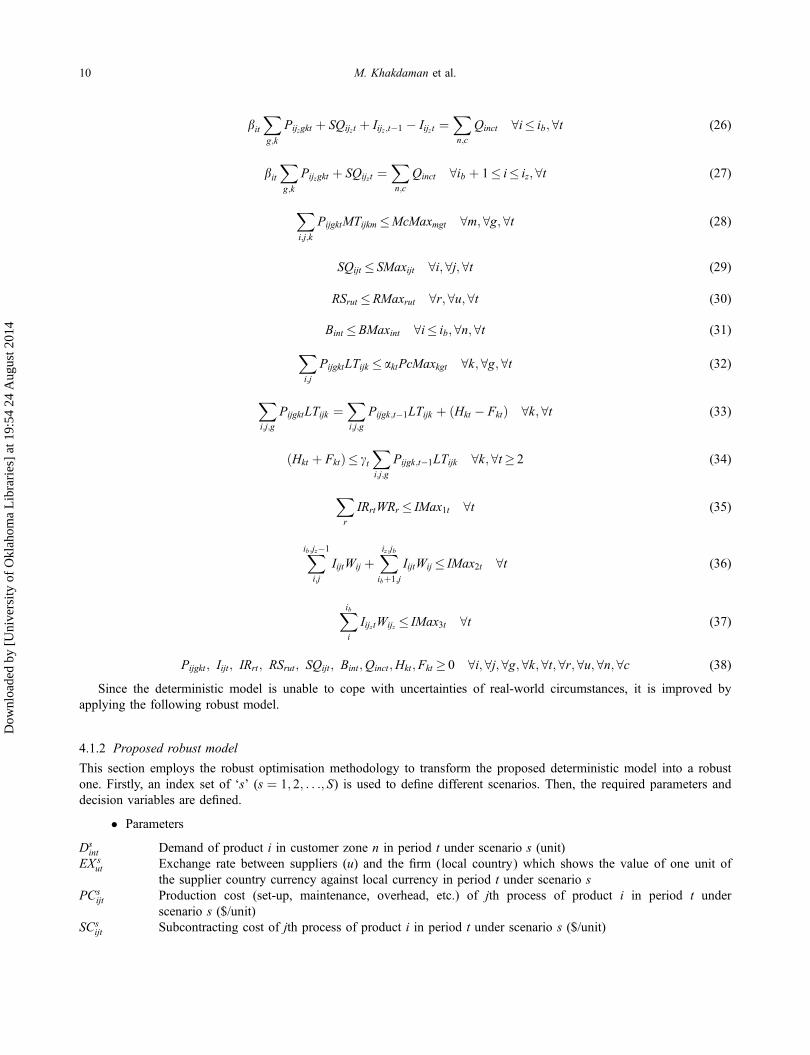
4.1.2 Proposed robust model

This section employs the robust optimisation methodology to transform the proposed deterministic model into a robustone. Firstly, an index set of ‘s’ (s ¼ 1; 2; . . .; S) is used to define different scenarios. Then, the required parameters anddecision variables are defined.

� Parameters

Dsint Demand of product i in customer zone n in period t under scenario s (unit)

EX sut Exchange rate between suppliers (u) and the firm (local country) which shows the value of one unit of

the supplier country currency against local currency in period t under scenario sPCs

ijt Production cost (set-up, maintenance, overhead, etc.) of jth process of product i in period t underscenario s ($/unit)

SCsijt Subcontracting cost of jth process of product i in period t under scenario s ($/unit)

10 M. Khakdaman et al.

Dow

nloa

ded

by [

Uni

vers

ity o

f O

klah

oma

Lib

rari

es]

at 1

9:54

24

Aug

ust 2

014

RCsrut Cost of raw material r (in terms of the currency of supplier country) procured from supplier u in period t

under scenario s ($/unit)ICs

ijt Inventory holding cost of product i that completed its jth process in period t under scenario s ($/unit)IRCs

rt Inventory holding cost of raw material r in period t under scenario s ($/unit)BCs

int Backorder cost of product i for customer n in period t under scenario s ($/unit)LCs

kgt Labour cost of k-type workers in production time g in period t under scenario s ($/man-hour)HtCs

kt Hiring (and training) cost of k-type workers in period t under scenario s ($/man-hour)FCs

kt Firing cost of k-type workers in period t under scenario s ($/man-hour)TCs

nct Average transportation cost of sending finished products to customer n by transportation mode c inperiod t under scenario s ($/unit)

qs Occurrence probability of scenario sk Weighting scale to measure the trade-off between risk and expected outcomex1;x2 Weighting penalty to trade-off solution for model robustness

� Decision variables

Bsint Quantity of finished product i ordered in period t by customer n which will be backordered for fulfilment

in future periods under scenario s (unit)Qs

inct Quantity of finished product i allocated to customer n by transportation mode c in period t under scenarios (unit)

ds�1int Underfulfilment (shortage) of MTS product i for customer n in period t under scenario s (unit)ds�2int Underfulfilment (shortage) of MTO product i for customer n in period t under scenario s (unit)dsþ1int Overfulfilment (storage) of MTS product i for customer n in period t under scenario s (unit)dsþ2int Overfulfilment (storage) of MTO product i for customer n in period t under scenario s (unit)hs Deviation for violation of the mean

In this model, Qsinct and Bs

int are control variables because they determine the optimal values of design variables. Inthe manufacturing environment, the quantities that are allocated to and backordered for each customer (Qs

inct and Bsint),

normally determine or control the production and subcontracting-related variables such as Pijgkt, SQijt , etc. Consideringthe defined scenarios, robust optimisation will find the best feasible values of the control variables and based on these,it will optimise the values of the design variables. As an example, consider two customers. If the solution recommendsthe fulfilment quantity (control variable) of the first customer to be more than the second one (less backorder for thefirst customer), more production quantity (design variable) will be needed for the first customer. It should be noted thatidentifying the correct control variables is important since they construct and adjust control constraints. In this regard,any violation of the control constraints leads the model to an infeasibility derived from the vector of error variablesds�1int, d

sþ1int, d

s�2int and dsþ2int. Here, we need hs as a variable to consider deviation from the mean in the objective function.

� Objective function

To be more convenient, we take the following abbreviations into account.

PCs Production costð Þ ¼Xi;j;g;k;t

PijgktPCsijt (39)

LCs Labour costð Þ ¼Xi;j;g;k;t

PijgktLTijkLCskgt þ

Xk;t

HktHtCskt þ FktFC

skt

� �(40)

ICs Inventory holding costð Þ ¼Xi;j;t

IijtICsijt þ

Xr;t

IRrtIRCsrt (41)

SCs Subcontracting costð Þ ¼Xi;j;t

SQijtSCsijt (42)

RCs Raw material costð Þ ¼Xr;u;t

EX sutRC

srutRSrut (43)

International Journal of Production Research 11

Dow

nloa

ded

by [

Uni

vers

ity o

f O

klah

oma

Lib

rari

es]

at 1

9:54

24

Aug

ust 2

014

TCs Transportation costð Þ ¼Xi;n;c;t

QsinctTC

snct (44)

BCs Backorder costð Þ ¼Xibi;n;t

BsintBC

sint (45)

The robust objective function for minimising the total costs is presented in Equation (46). The first part is theexpected value of the total costs which is used in the stochastic linear programming formulation. The second partmeasures the variance of the different scenario objectives from the expected mean of the total costs. The third term isthe infeasibility penalty function to penalise violations of the control constraints caused by some of the scenarios. In thispart, two separate x are defined to provide appropriate flexibility for penalising infeasibilities of MTS and MTO prod-ucts separately according to the decision-makers’ policies. Based on the model assumptions, since the shortage of MTSproducts is not allowed, any shortage of MTS products would lead the problem to an infeasible solution. Thus, the errorvector ds�1int is penalised in the third term of the objective function to punish the infeasibilities raised from underfulfil-ments of MTS products. As shortage and surplus of finished MTO products are not allowed in the model assumptions,the related infeasibilities measured by error vectors ds�2int and dsþ2int are punished using the weighting penalty x2.

Min total costs ¼ Min Z1 ¼Xs

qsðPCs þ ICs þ RCs þ LCs þ BCs þ SCs þ TCsÞ

þ kXs

qs

"PCs þ ICs þ RCs þ LCs þ BCs þ SCs þ TCsÞð

�Xs0

qs0 ðPCs0 þ ICs0 þ RCs0 þ LCs0 þ BCs0 þ SCs0 þ TCs0 Þ þ 2hs#

þXs

qsXibi

x1ds�1int þ

Xizibþ1

x2 ds�2int þ dsþ2int� � !

(46)

The second objective function (Equation (47)) is free of noise since it is constructed using fixed parameters anddesign variables rather than uncertain parameters and control variables. Thus, robust transformation is not required.However, to make the second objective function consistent with the first one, the objective function of minimisation ofthe machines inefficiency is used instead of maximisation of the machines efficiency.

Max machines efficiency ¼ Min machines inefficiency ¼ Min Z2

¼Xm;g;t

McMaxmgt �X

i;j;k;g;m;t

bitPijgktMTijkm

!=Xm;g;t

McMaxmgt

!(47)

� Constraints

Equation (48) is developed based on Equation (12) to maintain the different objective functions generated bydifferent scenarios as non-negative. For each scenario, Equation (48) illustrates that the difference between the total costand expected mean cost plus its deviation for violation of the mean should be non-negative. Equations (49) and (50) arethe most significant control constraints that are used to determine the quantity of MTS and MTO products allocated toeach customer, respectively. This allocation will determine the inventory level and the underfulfilments of marketdemand.

PCs þ ICs þ RCs þ LCs þ BCs þ SCs þ TCsð Þ �Xs0

qs0 ðPCs0 þ ICs0 þ RCs0 þ LCs0 þ BCs0 þ SCs0 þ TCs0 Þ þ hs � 0 8s

(48)

Dsint þ Bs

in;t�1 ¼Xc

Qsinct þ Bs

int þ ds�1int � dsþ1int 8i� ib; 8n; 8t; 8s (49)

12 M. Khakdaman et al.

Dow

nloa

ded

by [

Uni

vers

ity o

f O

klah

oma

Lib

rari

es]

at 1

9:54

24

Aug

ust 2

014

Dsint ¼

Xc

Qsinct þ ds�2int � dsþ2int 8ib þ 1� i� iz; 8n; 8t; 8s (50)

For MTS products (Equation (49)), it is noted that if the backordered quantity and total quantity of products trans-ferred to customers in period t (

Pc Q

sinct þ Bs

int) is greater than the market demand and backorders from the previousperiod (Ds

int þ Bsin;t�1Þ; then the stock of product i for customer n in period t will be equal to dsþ1int and under minimisa-

tion, the deviation ds�1int ¼ 0; whereas if Dsint þ Bs

in;t�1 is greater thanP

c Qsinct þ Bs

int, then dsþ1int ¼ 0 andds�1int ¼ Ds

int þ Bsin;t�1 � ðPc Q

sinct þ Bs

intÞ illustrating the underfulfilment of market demand which is an infeasible solu-tion. For MTO products (Equation (50)), if the total quantity of products transferred to customers in period t (

Pc Q

sinct)

is greater than the market demand (Dsint) then, under minimisation, the deviation ds�2int ¼ 0; and the stock of product i for

customer n in period t will be equal to dsþ2int ¼P

c Qsinct � Ds

int, which is an infeasible solution based on MTO productsassumptions; whereas if Ds

int is greater thanP

c Qsinct , then dsþ2int ¼ 0 and ds�2int ¼ Ds

int �P

c Qsinct indicating the underfulf-

ilment of market demand which is also an infeasible solution.The rest of the control constraints are shown in Equations (51)–(53) which are the modified versions of Equations

(26), (27) and (31), respectively. Equations (51) and (52) determine the total number of products which should be allo-cated for all of the customers in each scenario for MTS and MTO products, respectively. Since the backorder quantityof products is a control variable for each scenario, Equation (53) is applied to ensure that the number of backorderedproducts in each scenario would not exceed the maximum allowed quantity by decision-makers. Equation (54) is usedto make sure that all of the variables are non-negative.

bitXg;k

Pijzgkt þ SQijzt þ Iijz;t�1 � Iijzt ¼Xn;c

Qsinct 8i� ib; 8t; 8s (51)

bitXg;k

Pijzgkt þ SQijzt ¼Xn;c

Qsinct 8ib þ 1� i� iz; 8t; 8s (52)

Bsint �BMaxint 8i� ib; 8n; 8t; 8s (53)

Bsint; Qs

inct; ds�1int; ds�2int; dsþ1int; dsþ2int; hs � 0 8i; 8t; 8n; 8c; 8s (54)

To sum up, it should be stated that the final proposed robust model consists of Equations (46) and (47) as the multi-objective functions and Equations (20)–(23), (28)–(30), (32)–(38) and (48)–(54) as the constraints.

4.2 Solution procedure

Conventional deterministic optimisation approaches for tactical production planning problems are not capable of captur-ing their true dynamic behaviours. The ‘state-of-the-art’ of our solution procedure is using robust optimisation whichenables firms to handle the inevitable uncertainty of their business environment in a more practical manner. It is morebeneficial than standard probabilistic methods which are mostly hard to implement. Another advantage of our solutionprocedure is the applicability and effectiveness of the final solution. In deterministic approaches, one optimal solution isprovided for each variable, while our solution method creates a robust and near optimal plan, which remains valid overa practical range of variable values at a favourable and predictable cost. This robust property enables us to model andcapture the inherent uncertainty of complicated optimisation problems.

To solve the proposed multi-objective robust model, we used the following steps:

(1) As a result of conflicting objectives, our proposed robust model separates the problem into two models so thateach one includes one objective function and all of the related constraints.

(2) The first model aims to minimise the total costs consisting of Equation (46) as the objective function andEquations (20)–(23), (28)–(30), (32)–(38) and (48)–(54) as the constraints. To achieve the optimal solution forthe first model, appropriate values of penalties x1 and x2 should be determined through the trade-off betweenthe expected total costs and expected shortages. Using the case study data presented in the following section,we discuss this trade-off along with the solutions for the first model.

International Journal of Production Research 13

Dow

nloa

ded

by [

Uni

vers

ity o

f O

klah

oma

Lib

rari

es]

at 1

9:54

24

Aug

ust 2

014

(3) The second model which is constructed to maximise the total machines efficiency, includes Equation (47) asthe objective function and Equations (20)–(23), (28)–(30), (32)–(38) and (49)–(54) as the constraints. Weapply again the case study data to illustrate the usefulness of this model.

(4) In the last step, the Lp-Metric methodology is applied. Assume that Z�1 and Z�

2 are the optimum solution val-ues of the first and second models, then ZLp�Metric (Equation (55)) shows the final integrated objective func-tion.

Min ZLp�Metric ¼ uððZ1 � Z�1Þ=Z�

1Þ þ 1� uð ÞððZ2 � Z�2Þ=Z�

2Þ (55)

0�u� 1 (56)

It is worth noting that a key strength of the Lp-Metric methodology is that it provides a flexible tool to test differentweights for each objective function. This advantage is very useful for managers and decision-makers as it allows themto fine tune their optimisation models.

5. An illustrative case

We applied the proposed model in BALAN SANAAT Company which is one of the manufacturing leaders in producingdifferent types and sizes of load lifters. The company was established in 1984 in Iran aiming at producing some kindsof automatic and semi-automatic machines to increase the quality and speed of work activities. The core competency ofthe company is in the design and development of vehicle lifters, using electro-hydraulic and electro-mechanical systems.It is also capable of designing and producing stacking machines, antenna lifters and home facility lifters. Product charac-teristics like desirable quality, remarkable safety, fast installation, elegance and fineness have enabled the company toexport its products to some foreign countries like Turkey and India.

The main reason for selecting this company is that its production strategy is a mixture of MTS and MTO simulta-neously, which is consistent with our model. Some of the products are produced based on the predicted demand in adaily routine production (MTS strategy) while others are produced based on the confirmed customers’ order (MTO strat-egy). Among various product types, we selected two MTS and two MTO products for testing our novel model. Rawmaterials and components of these products are supplied from foreign countries like China and Germany as well as localmarkets. The raw materials are classified into seven categories which are iron sheets and shafts, aluminium sheets andshafts, tyres, hydraulic pumps, paint, standard parts like screws and nuts, and power control boxes.

In terms of production process, each product has five processes. Firstly, iron and aluminium sheets and shafts arecut and sent to the machining process. Then, machined parts are welded based on each product’s design drawings andsent to the painting process. Finally, all parts are assembled to form a completed product. In addition, there are threemachine centres for performing all processes. All of the activities related to cutting and machining processes are per-formed in the first machine centre. The second machine centre is dedicated for welding only. The last machine centre isdesigned to perform painting and assembling activities. With respect to human resources, there are around 45 skilledand 35 semi-skilled workers for producing all products in regular time and overtime. The finished products are trans-ported by trains, flights or trucks to satisfy local and international customers.

It should be noted that although most of the decision variables of the case study take integer values, some of themwhich are Hkt and Fkt take real values. Thus, in this case study, the proposed deterministic and robust models would bea mixed integer linear programming model. This case study contains four products (Table 1). Since products 3 and 4are MTO products, they are allowed to be produced up to the second process (machining) and after receiving thecustomers’ orders, the remaining processes will be performed. Thus, jb for both MTO products would be equal to 2.The index sets are as follows.

� Index sets

i Products, i ¼ 1&2 (MTS), 3&4 (MTO)j Processes, j ¼ 1 (Cutting), 2 (Machining), 3 (Welding), 4 (Painting), 5 (Assembling)m Machine centres, m ¼ 1 (Cut & Machine), 2 (Weld), 3 (Paint & Assemble)k Workers’ skill levels, k ¼ 1 (Skilled), 2 (Semi-skilled)r Raw material types, r ¼ 1 (Iron sheet & shaft), 2 (Aluminium sheet & shaft), 3 (Tyre), 4 (Hydraulic

pump), 5 (Paint), 6 (Standard parts (nut, screw, etc.)), 7 (Power control box)a Inventory types, a ¼ 1 (Raw material), 2 (WIP), 3 (Finished product)

14 M. Khakdaman et al.

Dow

nloa

ded

by [

Uni

vers

ity o

f O

klah

oma

Lib

rari

es]

at 1

9:54

24

Aug

ust 2

014

g Production time, g ¼ 1 (Regular time), 2 (Overtime)n Customers, n ¼ 1 (Local), 2 (India), 3 (Turkey)u Suppliers, u ¼ 1 (Local), 2 (China), 3 (Germany)c Transportation modes, c ¼ 1 (Road), 2 (Rail), 3 (Air)t Planning periods, t = 1,2,…,12

For the proposed robust model, four scenarios (Booming, Good, Fair and Poor) are applied for considering differentrange of uncertainties in the input data as well as different future economic situations in the local country. The Poor sce-nario signifies the most pessimistic future outcome and in contrast, the Booming scenario represents the extremely opti-mistic case. The Fair scenario is, in fact, the most expected scenario. According to the principles of robust optimisation,at least the most optimistic and most pessimistic situations should be considered in addition to the fair situation. In thisstudy, our four scenarios (index set: s = 1–4) include extremely optimistic (Booming), optimistic (Good), most expected(Fair) and extremely pessimistic (Poor) with an occurrence probability, qs of 0.15, 0.20, 0.40 and 0.25, respectively,such that the sum of all four probabilities is equal to 1. Numerous meetings were held with the senior managers of thecase company and based on their consensual estimation and prediction of the future economy outlook of the country,these four scenarios and their occurrence probabilities were established. More scenarios would provide more comprehen-sive results, but given the limitations in accessing the data of the case company, four scenarios would be accurateenough for robust optimisation. These scenarios are independent since each of them comprises a different set of dataand they are representatives of quite different future outcomes. All the required data were obtained from historicalrecords and forecasts of the case company.

Table 1. Product types and processes.

Products (i) Processes ( j)

Number 1 2 3 4 5

1 (MTS) Cutting Machining Welding Painting Assembling2 (MTS) Cutting Machining Welding Painting Assembling3 (MTO) Cutting Machining (jb ¼ 2Þ Welding Painting Assembling4 (MTO) Cutting Machining (jb ¼ 2Þ Welding Painting Assembling

Table 3. Optimal supply plan of raw material for the proposed deterministic model.

Raw material Supplier

Planning time period

1 2 3 4 5 6 7 8 9 10 11 12

1 2 1461 1463 1387 1428 1380 1467 1405 1472 1408 1474 1431 14042 1 38 12 71

2 1275 1275 1208 1264 1153 1229 1225 1275 1168 1272 1170 11513 2 132 132 144 128 156 120 112 124 148 116 144 1444 2 46 48 51 47 53 47 46 46 51 47 53 525 2 986 923 814 910 855 905 780 985 854 892 816 7836 2 1674 1743 1905 1733 2009 1857 1788 1699 1976 1827 2130 20677 2 38 39 41 36 46 34 30 33 43 34 42 42

Table 2. Model size and computation time.

Model type Objective function

No. of variables

No. of constraints Execution time (s)aInteger Continuous Total

Deterministic Min total costs 2016 385 2401 1235 11Robust Min total costs & Max machines efficiency 4896 391 5287 2033 69

aA computer with a Core (TM) i5 2.50 GHz CPU and 4.0 GB RAM was used.

International Journal of Production Research 15

Dow

nloa

ded

by [

Uni

vers

ity o

f O

klah

oma

Lib

rari

es]

at 1

9:54

24

Aug

ust 2

014

6. Results and discussion

Generally, using an effective linearised formulation (rather than a quadratic one) to represent the proposed robust modelhas helped to deal with its computational complexity. This approach has been proposed by Yu and Li (2000) andrecently demonstrated by Lalmazloumian et al. (2013). In addition, a powerful tool which is IBM ILOG CPLEX optimi-sation studio (version 12.3) was applied to handle its computation. CPLEX is capable of solving very complex mathe-matical programming problems such as the proposed robust model. As can be seen in Table 2, the proposed modelcontains a large number of decision variables and constraints. Using CPLEX, the model was successfully solved withina reasonable amount of computation time (see Table 2).

6.1 Results of the proposed deterministic model

As the first evaluation of the proposed deterministic model, we solved it using CPLEX to obtain the minimum total costof the proposed model based on our case study data. Here, only the objective function of minimising total costs(Equation (18)) is used with all of the related constraints (Equations (20)–(38)) to achieve the objective function valueof $1,367,696.84. The optimum production plans are depicted in Tables 3–9. It should be noted that throughout thisstudy, for the purpose of making tables clearer, the decision variables with an optimal value of zero (for example,inventories of raw material, WIP and finished product) are not shown.

6.2 Results of the proposed robust model

Subsequently, the proposed robust model is solved based on the solution procedure presented in Section 4.2.

6.2.1 Results for minimising total costs

Before running the model in the CPLEX software to obtain the optimal solution of the robust cost model, we allocatedthe best value for the infeasibility penalty weights x1 and x2 for MTS and MTO products respectively. The role ofweights x1 and x2 in the objective function is to find an optimal trade-off between solution robustness and modelrobustness. Here, since fulfilling customers’ demands of MTO products is more important than MTS ones in the pro-posed MTS–MTO strategy, we assume the value of x2 as one time more than x1 to penalise the underfulfilment ofMTO products more heavily. Thus, based on the above decision, we solve the proposed robust cost model several times,each time using different values of x1 and x2 so that at the end, we can consider the best values of x1 and x2 for theproposed final robust model. We applied the data in Table 10 to draw the trade-off graph in Figure 1. To demonstratethe procedure of drawing Figure 1, for instance, when we solve the proposed robust cost model by setting x1 = 1200and x2 = 2400, we obtain the optimal solution with an objective function of $1,075,030 and expected underfulfilmentsof 214 and 292 units of MTS and MTO products, respectively. Thus, with the expected total cost of $1,075,030 wewould expect to have 506 units of products as shortage. As a reminder, the expected value of underfulfilments for eachset of x1 and x2 is calculated by

P2i¼1 qsd

s�1int þ

P4i¼3 qsd

s�2int.

Table 4. Optimal product allocation plan for the proposed deterministic model.

Product Customer Transportation Mode

Planning time period

1 2 3 4 5 6 7 8 9 10 11 12

1 1 2 2 5 2 2 6 1 2 3 4 5 32 1 2 1 2 1 2 2 1 33 2 1 1 2 1 3 2 1 1

2 1 2 7 6 7 7 4 4 6 8 3 3 42 1 2 1 2 2 2 3 33 2 5 5 5 4 3 1 2 4 3 6 1 1

3 1 2 11 10 11 9 8 13 11 12 7 11 12 102 1 5 5 4 5 6 3 5 7 6 4 5 43 2 1 2 2 1 2 1 1 3 2

4 1 2 7 5 3 6 7 8 5 7 9 4 6 72 1 2 2 2 1 1 1 3 3 1 23 2 3 2 2 3 3 4 1 3 2 3

16 M. Khakdaman et al.

Dow

nloa

ded

by [

Uni

vers

ity o

f O

klah

oma

Lib

rari

es]

at 1

9:54

24

Aug

ust 2

014

To illustrate the concept of trade-off between solution robustness and model robustness in our case study, we recallthe robust optimisation methodology as explained earlier. Robust optimisation allows infeasibilities in the control con-straints by penalising them. In this regard, when x1 =x2 = 0, due to the minimisation of objectives, ds�1int and ds�2int inconstraints 49 and 50 would be equal to Ds

int, respectively. Therefore, no production is advised in the optimal plan

Table 5. Optimal production plan in regular time for the proposed deterministic model.

Product Process Labour

Planning time period

1 2 3 4 5 6 7 8 9 10 11 12

1 1 1 5 3 4 6 2 4 3 52 4 5 1 6

2 1 1 2 33 1 5 6 3 2 2 54 1 4 4 4

2 5 2 5 8 4 4 6 6 65 1 3 6 8 4 4 6 2

2 1 62 1 1 14 11 12 9 6 8

2 1 1 1 12 5 4 42 1 1 3 5 6 3 4 7 4 4 5

2 23 1 6 12 8 7 7 7 9 4

2 6 9 1 3 4 14 1 6 12 3 7 8 1 3 3 5

2 3 6 1 11 15 1 3 5 13 5 7 8 9 5

2 7 3 93 1 1 17 1 14 4 6 20 4 7 16

2 17 15 12 1 17 17 15 16 14 17 18 18 11 18 15 123 1 15 15 11 16 13 17 11 20 10 9 16 16

2 1 3 4 54 1 17 15 17 18 4 17 1

2 17 16 175 1 13 15 15 12 14 17 16 15 14 13 15 14

4 1 1 8 6 1 3 1 102 12 10 1 1 10 12 9

2 1 1 1 7 1 2 1 8 1 23 1 1 11 5 12

2 7 6 6 10 94 1 11 9 7 1 11 13 9 12 9 10 6

2 35 2 1 4 8 2 9 9

Table 6. Optimal subcontracting plan for the proposed deterministic model.

Product Process

Planning time period

1 2 3 4 5 6 7 8 9 10 11 12

1 2 5 5 5 4 5 4 4 5 5 4 33 1 25 3

2 2 11 7 3 7 4 3 3 12 2 43 5 4 2 1 54 2 4 4 4 4 4 4 4 4 4 4 4 4

3 11 9 4 1 10 74 1 15 11 9 3 10 3 11 6 10 4 9 1

International Journal of Production Research 17

Dow

nloa

ded

by [

Uni

vers

ity o

f O

klah

oma

Lib

rari

es]

at 1

9:54

24

Aug

ust 2

014

Table 7. Optimal production plan in overtime for the proposed deterministic model.

Product Process Labour

Planning time period

1 2 3 4 5 6 7 8 9 10 11 12

1 1 1 2 2 32 6

2 1 1 3 23 1 4 7 4 6 6 6

2 24 1 1

2 25 1 2 5 4 1 4

2 1 12 1 1 9

2 12 4 12 1 2 2 4 2 3 13 1 8 6 5 9 24 1 3

2 11 13 5 6 65 1 7 9 7 4 1 4

2 7 13 1 1 15 12 12 10 18 10

2 1 2 3 2 43 1 1 2 4 1 4 4 14 1 14 10 15

2 20 15 1 3 2 5 2 2

4 1 1 1 9 102 1 2 3 8

2 1 7 5 3 5 8 5 5 5 33 1 2

2 74 1 9 65 1 8

Table 8. Optimal hiring plan for the proposed deterministic model.

Hired labour

Planning time period

1 2 3 4 5 6 7 8 9 10 11 12

1 1468 10.7 1.2 0.42 209 2.5 25 44.5 6.9 6.9

Table 9. Optimal backordering plan for the proposed deterministic model.

Product Customer

Planning time period

1 2 3 4 5 6 7 8 9 10 11 12

1 1 1 1 1 1 12 1 1

2 1 1 1 12 1 1

18 M. Khakdaman et al.

Dow

nloa

ded

by [

Uni

vers

ity o

f O

klah

oma

Lib

rari

es]

at 1

9:54

24

Aug

ust 2

014

Table 10. Data associated with trade-off between cost and shortage.

x1 0 300 600 900 1200 1500 1800 2100 2400 2700x2 0 600 1200 1800 2400 3000 3600 4200 4800 5400ds�1int 221 219 219 218 214 210 195 155 123 112ds�2int 405 405 338 307 292 280 205 151 145 143Sum 626 624 557 525 506 490 400 306 268 255Objective

function0 291,105 577,258 830,718 1,075,030 1,312,212 1,539,771 1,704,294 1,838,778 1,964,321

x1 3000 3300 3600 3900 4200 4500 4800 5100 5400x2 6000 6600 7200 7800 8400 9000 9600 10,200 10,800ds�1int 97 93 84 82 78 74 69 65 62ds�2int 142 141 137 136 133 132 130 125 120Sum 239 234 221 218 211 206 199 190 182Objective

function2,082,798 2,198,803 2,311,403 2,425,996 2,542,714 2,649,587 2,762,959 2,865,411 2,968,411

Table 11. Optimal raw material supply plan for the proposed final robust model.

Raw material Supplier

Planning time period

1 2 3 4 5 6 7 8 9 10 11 12

1 2 1208 1775 1237 1309 1331 1390 1229 1123 1441 1219 1101 12812 1 1514 337

2 935 338 1061 1094 1123 1149 1275 740 1220 883 751 9503 2 140 160 176 160 168 144 160 172 168 140 156 1364 1 1

2 47 52 53 50 54 52 52 52 54 48 51 505 2 799 855 791 795 711 766 761 528 808 818 596 6576 2 1835 1916 1844 1822 2118 2156 1919 1708 2241 1844 1875 20587 1 3 1 37 1

2 42 47 51 41 51 6 49 47 50 44 51 40

Figure 1. Trade-off between solution robustness and model robustness.

International Journal of Production Research 19

Dow

nloa

ded

by [

Uni

vers

ity o

f O

klah

oma

Lib

rari

es]

at 1

9:54

24

Aug

ust 2

014

which results in reaching the total underfulfilment at the highest value. It is safe to argue that this plan cannot beadopted. Thus, testing the proposed robust cost model with various x1 and x2 becomes inevitable. Hence, as illustratedin Figure 1, we can trade-off cost and shortage as follows: As the weights x1 and x2 increase, the expected total costrepresenting solution robustness increases significantly, and the expected underfulfilment representing model robustness

Table 12. Optimal hiring plan for the proposed final robust model.

Hired labour

Planning time period

1 2 3 4 5 6 7 8 9 10 11 12

1 972.1 22.1 80.6 193.8 97.12 772.1 61.3 147.3 67.3 81.2 182.0 228.1

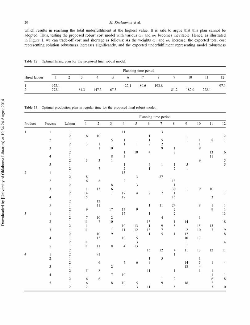
Table 13. Optimal production plan in regular time for the proposed final robust model.

Product Process Labour

Planning time period

1 2 3 4 5 6 7 8 9 10 11 12

1 1 1 11 32 6 10 1 1 2

2 1 5 1 1 5 1 1 8 12 3 1 1 1 2 2 1

3 1 1 10 9 1 92 1 10 4 3 13 6

4 1 8 3 112 3 3 1 9 5

5 1 1 6 1 1 5 52 7 2 1 2 1

2 1 1 132 8 3 27

2 1 6 8 2 132 8 3 1

3 1 1 13 6 30 1 9 102 14 1 17 4 2 7 1 1

4 1 15 17 15 32 12

5 1 11 1 11 24 8 1 12 9 17 17 9 2 9 1

3 1 1 17 1 2 132 7 10 2 4 1

2 1 11 7 10 13 1 14 182 1 10 13 1 9 8 15 13

3 1 11 1 11 12 13 7 2 10 7 92 10 9 1 1 5 1 12 8

4 1 15 10 5 10 172 11 3 1 14

5 1 11 11 8 4 13 12 15 12 4 11 13 12 11

4 1 2 91 12 1 1 5 1

2 6 7 6 9 14 5 1 43 1 2 18 4

2 5 8 11 1 1 14 1 7 10 1 1

2 6 6 1 2 6 85 1 6 8 10 5 9 18 2

2 2 3 11 5 3 10

20 M. Khakdaman et al.

Dow

nloa

ded

by [

Uni

vers

ity o

f O

klah

oma

Lib

rari

es]

at 1

9:54

24

Aug

ust 2

014

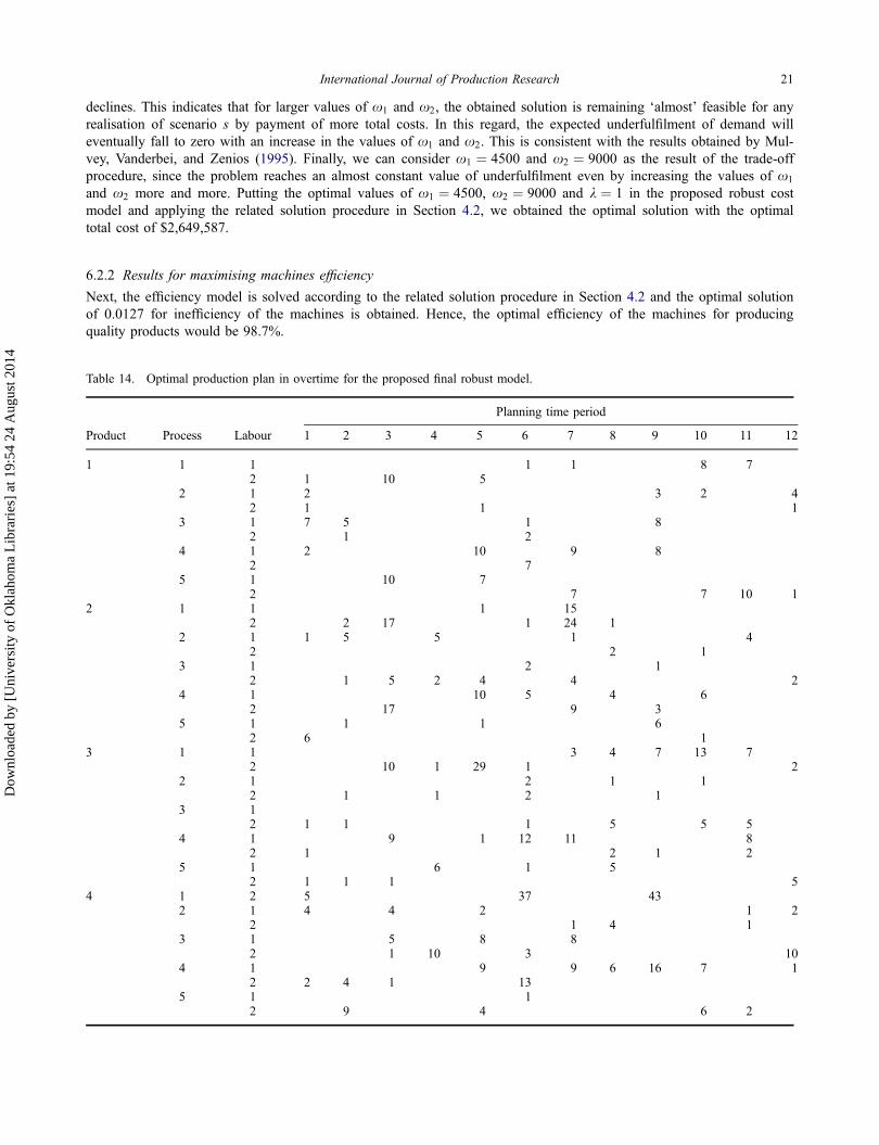
declines. This indicates that for larger values of x1 and x2, the obtained solution is remaining ‘almost’ feasible for anyrealisation of scenario s by payment of more total costs. In this regard, the expected underfulfilment of demand willeventually fall to zero with an increase in the values of x1 and x2. This is consistent with the results obtained by Mul-vey, Vanderbei, and Zenios (1995). Finally, we can consider x1 ¼ 4500 and x2 ¼ 9000 as the result of the trade-offprocedure, since the problem reaches an almost constant value of underfulfilment even by increasing the values of x1

and x2 more and more. Putting the optimal values of x1 ¼ 4500, x2 ¼ 9000 and k ¼ 1 in the proposed robust costmodel and applying the related solution procedure in Section 4.2, we obtained the optimal solution with the optimaltotal cost of $2,649,587.

6.2.2 Results for maximising machines efficiency

Next, the efficiency model is solved according to the related solution procedure in Section 4.2 and the optimal solutionof 0.0127 for inefficiency of the machines is obtained. Hence, the optimal efficiency of the machines for producingquality products would be 98.7%.

Table 14. Optimal production plan in overtime for the proposed final robust model.

Product Process Labour

Planning time period

1 2 3 4 5 6 7 8 9 10 11 12

1 1 1 1 1 8 72 1 10 5

2 1 2 3 2 42 1 1 1

3 1 7 5 1 82 1 2

4 1 2 10 9 82 7

5 1 10 72 7 7 10 1

2 1 1 1 152 2 17 1 24 1

2 1 1 5 5 1 42 2 1

3 1 2 12 1 5 2 4 4 2

4 1 10 5 4 62 17 9 3

5 1 1 1 62 6 1

3 1 1 3 4 7 13 72 10 1 29 1 2

2 1 2 1 12 1 1 2 1

3 12 1 1 1 5 5 5

4 1 9 1 12 11 82 1 2 1 2

5 1 6 1 52 1 1 1 5

4 1 2 5 37 432 1 4 4 2 1 2

2 1 4 13 1 5 8 8

2 1 10 3 104 1 9 9 6 16 7 1

2 2 4 1 135 1 1

2 9 4 6 2

International Journal of Production Research 21

Dow

nloa

ded

by [

Uni

vers

ity o

f O

klah

oma

Lib

rari

es]

at 1

9:54

24

Aug

ust 2

014

6.2.3 Results for integrated objective functions

This part of the analysis uses the obtained optimal values of both objective functions (see Sections 6.2.1 and 6.2.2) andputs them into the Lp-Metric objective function (our final integrated objective function of the proposed robust model).In this regard, we apply Zi to show the optimal value of both objective functions after solving the integrated model. Inaddition, the parameter u is considered as 0.7 since the cost objective is more important than the efficiency objectivewhen we asked the top managers of the case study company. To sum up, the following settings are utilised.

x1 ¼ 4500; x2 ¼ 9000; k ¼ 1; Z�1 ¼ 2,649,587; Z�

2 ¼ 0:0127; u ¼ 0:7

Using the above settings, the proposed final robust model is solved using the CPLEX software yielding a final objectivefunction value of 0.07. Since the objective function is minimising the total costs and machines inefficiency, a value for theLp-Metric objective function nearer to zero would be desirable. Based on the optimal solution, the optimum values of the

Table 16. Optimal backordering plan for the proposed final robust model.

Product Customer Scenario

Planning time period

1 2 3 4 5 6 7 8 9 10 11 12

1 1 Booming 1 1 1 1Good 1 1 1 1 1 1 1Fair 1 1

2 Booming 1 1Good 1 1 1 1 1Fair 1 1 1Poor 1

2 1 Booming 1 1Good 1 1 1 1Fair 1 1 1 1 1 1

2 Booming 1 1Good 1 1Fair 1 1 1 1Poor 1 1 1

Table 15. Optimal subcontracting plan for the proposed final robust model.

Product Process

Planning time period

1 2 3 4 5 6 7 8 9 10 11 12

1 1 4 3 1 6 6 6 6 2 1 6 42 5 5 5 4 4 3 1 4 4 5 53 24 2 1 3 15 3 3 2

2 1 11 12 2 11 11 2 12 3 32 8 5 10 14 6 4 14 14 10 4 7 23 3 1 44 2 12 3 3 7 35 4 5

3 1 5 5 1 6 6 3 6 32 7 3 13 4 3 4 1 2 1 14 1 1 4 6 1 8 3 3 45 3 1 1 2 1 3 4 1 2

4 1 3 7 5 7 7 72 4 4 4 3 4 4 4 4 4 1 4 43 3 2 4 2 7 2 64 3 1 25 1 2 1 3 1

22 M. Khakdaman et al.

Dow

nloa

ded

by [

Uni

vers

ity o

f O

klah

oma

Lib

rari

es]

at 1

9:54

24

Aug

ust 2

014

total costs and machines inefficiency would be $3,654,430.71 and 0.0041 respectively. Besides this, the optimal expectedunderfulfilments for MTS and MTO products would be 63 and 121 units of products, respectively.

Tables 11–23 show the optimal plans of the proposed final robust model. As an illustrative example, Table 13 showsthat skilled workers should produce 8, 3 and 11 semi-finished products of the painting process (4th process) of the firstproduct in periods 3, 4 and 11 respectively. Notably, in both the regular time and overtime production plans (Tables 13and 14), the first process of the fourth product should be performed only by semi-skilled workers. The underfulfilmentsof market demand for MTS products in all scenarios are shown in Table 22. For instance, we expect to have one unit ofshortage in each of the Good, Fair and Poor scenarios for the third customer of the first product in period one.

Comparing the quantity of underfulfilments of market demand for MTS and MTO products in the Poor scenariohighlights the fact that the company’s managers could expect to handle almost all the orders of MTO products; however,they will certainly have some shortages for MTS products. This issue is expected because we define the penalty weightx for MTO products as one time more than MTS ones, since responsiveness for MTO products is assumed to be moreimportant than MTS ones.

Another issue that the company’s managers should take into account is that although the quantity of underfulfilmentsof both products is reduced to less than one-third by applying the robust optimisation technique (consider Table 10where the total expected underfulfilment reduces from 626 to 206 by increasing the penalty factor x), increasing the

Table 17. Optimal allocation plan of product 1 for the proposed final robust model.

Customer Transportation Mode Scenario

Planning time period

1 2 3 4 5 6 7 8 9 10 11 12

1 2 Booming 3 7 5 3 10 7 4 5 13Good 3 7 5 3 10 4 6 1 6 9Fair 1 7 6 3 8 3 7 5 4 12 3Poor 2 6 7 3 8 5 7 2 6 12

2 1 Booming 2Good 1 1Fair 2 3 1 2 1 3Poor 1 1 2 1 1 1 6

3 Good 4 33 1 Booming 5 3 6

Good 1 62 Booming 4

Good 1 3 3 1Fair 1 1 4 4 1Poor 1 1 2 2 1 4

3 Booming 5Good 4

Table 18. Optimal allocation plan of product 2 for the proposed final robust model.

Customer Transportation Mode Scenario

Planning time period

1 2 3 4 5 6 7 8 9 10 11 12

1 2 Booming 15 12 17 17 5 5 8 31 6 9 9Good 9 9 11 12 6 5 11 31 2 9 3Fair 8 7 11 12 4 5 9 27 6 1 3 2Poor 12 7 13 12 6 4 8 27 1 8

2 1 Fair 2 1 3 2Poor 1 1 2 2 1 1 1 3

2 Fair 13 1 Good 3

Fair 42 Booming 5 3 3

Good 6 6 5 4 4 9Fair 5 5 5 4 3 2 6 6 1Poor 2 4 4 3 2 2 3 5 6 1 3

International Journal of Production Research 23

Dow

nloa

ded

by [

Uni

vers

ity o

f O

klah

oma

Lib

rari

es]

at 1

9:54

24

Aug

ust 2

014

Table 19. Optimal allocation plan of product 3 for the proposed final robust model.

Customer Transportation Mode Scenario

Planning time period

1 2 3 4 5 6 7 8 9 10 11 12

1 1 Poor 122 Booming 12 15 10 11 13 18 12 10 15 17 13 18

Good 12 15 10 11 12 18 12 10 11 17 13 15Fair 11 10 10 9 8 14 11 10 7 11 12 12Poor 7 9 7 5 8 15 7 4 9 6

3 Poor 132 1 Good 3

Fair 3 5 3 6 1 4Poor 4 4 3 4 5 2 3 5 5 3 7 3

2 Fair 33 1 Good 3

Fair 12 Good 1 1

Fair 1 2 2 1 2 3 2Poor 1 2 2 1 2 1 1 2 2

Table 20. Optimal allocation plan of product 4 for the proposed final robust model.

Customer Transportation Mode Scenario

Planning time period

1 2 3 4 5 6 7 8 9 10 11 12

1 2 Booming 8 10 8 10 12 14 10 8 18 7 7 10Good 8 8 5 9 11 12 8 8 14 6 7 10Fair 5 6 4 6 8 9 9 7 9 4 4 8Poor 4 6 4 8 9 10 10 6 16 3 4 8

2 1 Good 4Fair 2 2 1 1 1 3 1 2Poor 2 2 2 1 1 2 2 1 2

3 2 Good 2 3 1 1 2 2 1Fair 3 2 2 3 3 4 1 1 6 2 3Poor 2 2 2 2 2 3 2 2 2

Table 21. Optimal inventory plan of WIP and finished product for the proposed final robust model.

Product Process

Planning time period

1 2 3 4 5 6 7 8 9 10 11 12

1 1 3 2 2 3 52 4 3 3 6 2 14 4 1 25 1 3

2 1 4 1 3 62 31 21 12 1 12 1 2 4 2 1 5 4 13 5 2 1 45 1

3 1 1 8 23 7 1 22 2 1 1 1

4 1 4 32 29 22 52 25 17 12 41 49 1

24 M. Khakdaman et al.

Dow

nloa

ded

by [

Uni

vers

ity o

f O

klah

oma

Lib

rari

es]

at 1

9:54

24

Aug

ust 2

014

production resources would be the only way to reduce the almost constant rate of the total expected underfulfilments(see Figure 1) to zero if they are very risk-averse.

Essentially, the impact of choosing different amounts of weighting factor u by decision-makers should be discussed.By considering various amounts of u, a trade-off between the two objective functions, total costs and machinesefficiency, is conducted to depict a spectrum of different possible future situations for decision-makers. In this regard,

Table 22. Underfulfilments of market demand for MTS products for the proposed final robust model.

Product Customer Scenario

Planning time period

1 2 3 4 5 6 7 8 9 10 11 12

1 1 Booming 3 1 3 4 9 5Good 2 1 5 5Fair 1Poor 2 2

2 Booming 4 2 4 3 1 2 2 6 2 3 2 7Good 3 1 2 1 2 5 1 5Fair 2Poor 1 2

3 Booming 2 2 3 3 1 3 2Good 1 1 3 1 1 1Fair 1 2 1Poor 1 2

2 1 Booming 4 2 29 1Good 2 4Fair 2Poor 3

2 Booming 6 2 4 4 4 4 3 2 5 6 3 2Good 4 2 2 3 3 3 1 2 3 4 2 1Fair 2 1 1 2Poor 1

3 Booming 8 7 9 6 3 6 6 9 2Good 3 2 3 5 1 1Fair 1 3Poor 1

Table 23. Underfulfilments of market demand for MTO products for the proposed final robust model.

Product Customer Scenario

Planning time period

1 2 3 4 5 6 7 8 9 10 11 12

3 1 Booming 10 5 13 7 3 8 13 11 5 11 2Good 5 7 3 2 5 8 5Fair 1 2Poor 2

2 Booming 11 12 8 10 12 7 10 14 11 8 10 8Good 8 8 6 8 9 5 8 11 6 6 8 6Fair 5 2 4 5 1 5 7 1 4

3 Booming 4 5 2 4 3 2 3 2 3 5 2 3Good 2 3 2 3 1 1 3 1 4 1Fair 1 1

4 1 Booming 6 2 2 2 6 1 5 4Good 3 5 2 1Fair 2 2

2 Booming 5 4 6 3 2 2 3 3 6 6 2 4Good 3 3 3 2 2 2 2 1 1 5 2 3Fair 2 2 1

3 Booming 5 4 5 5 5 6 3 5 2 6 5 2Good 4 1 3 3 3 4 1 2 4 1Fair 2

International Journal of Production Research 25

Dow

nloa

ded

by [

Uni

vers

ity o

f O

klah

oma

Lib

rari

es]

at 1

9:54

24

Aug

ust 2

014

Table

24.

Dataof

trade-offbetweentotalcostsandmachinesefficiency.

u1

0.95

0.9

0.8

0.7

0.6

0.5

0.4

0.3

0.2

0.1

01�u

00.05

0.1

0.2

0.3

0.4

0.5

0.6

0.7

0.8

0.9

1Inefficiency

0.29

0.01

50.00

30.00

20.00

40.00

30.00

50.00

40.00

60.00

70.00

80.00

9Efficiency

71.0

98.5

99.7

99.8

99.6

99.7

99.5

99.6

99.4

99.3

99.2

99.1

Total

Costs

2,83

4,78

02,89

7,26

13,07

8,33

93,40

9,61

83,65

4,43

04,31

3,42

94,43

5,49

95,30

7,50

15,70

0,86

75,92

7,39

97,91

0,96

18,78

7,47

3

26 M. Khakdaman et al.

Dow

nloa

ded

by [

Uni

vers

ity o

f O

klah

oma

Lib

rari

es]

at 1

9:54

24

Aug

ust 2

014

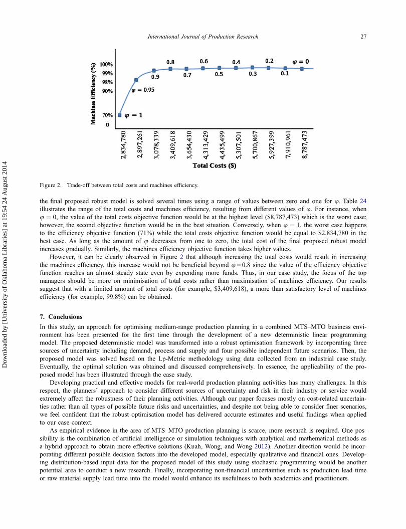
the final proposed robust model is solved several times using a range of values between zero and one for u. Table 24illustrates the range of the total costs and machines efficiency, resulting from different values of u. For instance, whenu ¼ 0, the value of the total costs objective function would be at the highest level ($8,787,473) which is the worst case;however, the second objective function would be in the best situation. Conversely, when u ¼ 1, the worst case happensto the efficiency objective function (71%) while the total costs objective function would be equal to $2,834,780 in thebest case. As long as the amount of u decreases from one to zero, the total cost of the final proposed robust modelincreases gradually. Similarly, the machines efficiency objective function takes higher values.

However, it can be clearly observed in Figure 2 that although increasing the total costs would result in increasingthe machines efficiency, this increase would not be beneficial beyond u = 0.8 since the value of the efficiency objectivefunction reaches an almost steady state even by expending more funds. Thus, in our case study, the focus of the topmanagers should be more on minimisation of total costs rather than maximisation of machines efficiency. Our resultssuggest that with a limited amount of total costs (for example, $3,409,618), a more than satisfactory level of machinesefficiency (for example, 99.8%) can be obtained.

7. Conclusions

In this study, an approach for optimising medium-range production planning in a combined MTS–MTO business envi-ronment has been presented for the first time through the development of a new deterministic linear programmingmodel. The proposed deterministic model was transformed into a robust optimisation framework by incorporating threesources of uncertainty including demand, process and supply and four possible independent future scenarios. Then, theproposed model was solved based on the Lp-Metric methodology using data collected from an industrial case study.Eventually, the optimal solution was obtained and discussed comprehensively. In essence, the applicability of the pro-posed model has been illustrated through the case study.

Developing practical and effective models for real-world production planning activities has many challenges. In thisrespect, the planners’ approach to consider different sources of uncertainty and risk in their industry or service wouldextremely affect the robustness of their planning activities. Although our paper focuses mostly on cost-related uncertain-ties rather than all types of possible future risks and uncertainties, and despite not being able to consider finer scenarios,we feel confident that the robust optimisation model has delivered accurate estimates and useful findings when appliedto our case context.

As empirical evidence in the area of MTS–MTO production planning is scarce, more research is required. One pos-sibility is the combination of artificial intelligence or simulation techniques with analytical and mathematical methods asa hybrid approach to obtain more effective solutions (Kuah, Wong, and Wong 2012). Another direction would be incor-porating different possible decision factors into the developed model, especially qualitative and financial ones. Develop-ing distribution-based input data for the proposed model of this study using stochastic programming would be anotherpotential area to conduct a new research. Finally, incorporating non-financial uncertainties such as production lead timeor raw material supply lead time into the model would enhance its usefulness to both academics and practitioners.

Figure 2. Trade-off between total costs and machines efficiency.

International Journal of Production Research 27

Dow

nloa

ded

by [

Uni

vers

ity o

f O

klah

oma

Lib

rari

es]

at 1

9:54

24

Aug

ust 2

014

References

Aghezzaf, E.-H., C. Sitompul, and N. M. Najid. 2010. “Models for Robust Tactical Planning in Multi-stage Production Systems withUncertain Demands.” Computers & Operations Research 37 (5): 880–889.

Akif Bakir, M., and M. D. Byrne. 1998. “Stochastic Linear Optimisation of an MPMP Production Planning Model.” InternationalJournal of Production Economics 55 (1): 87–96.

Al-e-Hashem, S. M. J. M., M. B. Aryanezhad, and S. J. Sadjadi. 2012. “An Efficient Algorithm to Solve a Multi-objective RobustAggregate Production Planning in an Uncertain Environment.” The International Journal of Advanced Manufacturing Technol-ogy 58 (5–8): 765–782.

Al-e-Hashem, S. M. J. M., H. Malekly, and M. B. Aryanezhad. 2011. “A Multi-objective Robust Optimization Model for Multi-product Multi-site Aggregate Production Planning in a Supply Chain under Uncertainty.” International Journal of ProductionEconomics 134 (1): 28–42.

Aryanezhad, M. B., A. S. Kheirkhah, V. Deljoo, and S. M. J. Mirzapour Al-e-hashem. 2009. “Designing Safe Job Rotation SchedulesBased upon Workers’ Skills.” The International Journal of Advanced Manufacturing Technology 41 (1–2): 193–199.

Bemelmans, R. 1986. The Capacity Aspect of Inventories. Berlin: Springer.Billington, P. J., J. O. McClain, and L. J. Thomas. 1983. “Mathematical Programming Approaches to Capacity-constrained MRP Sys-

tems: Review, Formulation and Problem Reduction.” Management Science 29 (10): 1126–1141.Byrne, M. D., and M. A. Bakir. 1999. “Production Planning Using a Hybrid Simulation – Analytical Approach.” International Jour-

nal of Production Economics 59 (1–3): 305–311.Carr, S. A., A. R. Güllü, P. L. Jackson, and J. A. Muckstadt. 1993. An Exact Analysis of a Production-inventory Strategy for Indus-

trial Suppliers. Working Paper. Cornell University.Chopra, S., and P. Meindl. 2010. Supply Chain Management: Strategy, Planning and Operation. Upper Saddle River, NJ: Pearson-

Prentice Hall.Dai, L., L. Fan, and L. Sun. 2003. “Aggregate Production Planning Utilizing a Fuzzy Linear Programming.” Transactions of the Soci-

ety for Design and Process Science 7 (4): 81–95.Garcia-Sabater, J. P., J. Maheut, and J. J. Garcia-Sabater. 2009. “A Decision Support System for Aggregate Production Planning

Based on MILP: A Case Study from the Automotive Industry.” In Proceedings of the International Conference on Computersand Industrial Engineering, France, 366–371.

Genin, P., A. Thomas, and S. Lamouri. 2007. “How to Manage Robust Tactical Planning with an APS (Advanced Planning Sys-tems).” Journal of Intelligent Manufacturing 18 (2): 209–221.

Goetschalckx, M., C. J. Vidal, and K. Dogan. 2002. “Modeling and Design of Global Logistics Systems: A Review of IntegratedStrategic and Tactical Models and Design Algorithms.” European Journal of Operational Research 143 (1): 1–18.

Gupta, A., and C. D. Maranas. 2003. “Managing Demand Uncertainty in Supply Chain Planning.” Computers & Chemical Engineer-ing 27 (8–9): 1219–1227.

Hax, A. C., and D. Candea. 1984. Production and Inventory Management. Englewood Cliffs, NJ: Pearson-Prentice Hall.Jamalnia, A., and M. A. Soukhakian. 2009. “A Hybrid Fuzzy Goal Programming Approach with Different Goal Priorities to Aggre-

gate Production Planning.” Computers & Industrial Engineering 56 (4): 1474–1486.Kallrath, J. 2005. “Solving Planning and Design Problems in the Process Industry Using Mixed Integer and Global Optimization.”

Annals of Operations Research 140 (1): 339–373.Kazaz, B., M. Dada, and H. Moskowitz. 2005. “Global Production Planning under Exchange-rate Uncertainty.” Management Science

51 (7): 1101–1119.Kazemi Zanjani, M., D. Ait-Kadi, and M. Nourelfath. 2010. “Robust Production Planning in a Manufacturing Environment with Ran-

dom Yield: A Case in Sawmill Production Planning.” European Journal of Operational Research 201 (3): 882–891.Kazemi Zanjani, M., M. Nourelfath, and D. Ait-Kadi. 2010. “A Multi-stage Stochastic Programming Approach for Production Plan-

ning with Uncertainty in the Quality of Raw Materials and Demand.” International Journal of Production Research 48 (16):4701–4723.

Kuah, C. T., K. Y. Wong, and W. P. Wong. 2012. “Monte Carlo Data Envelopment Analysis with Genetic Algorithm for KnowledgeManagement Performance Measurement.” Expert Systems with Applications 39 (10): 9348–9358.

Lalmazloumian, M., K. Y. Wong, K. Govindan, and D. Kannan. 2013. “A Robust Optimization Model for Agile and Build-to-orderSupply Chain Planning under Uncertainties.” Annals of Operations Research. doi:10.1007/s10479-013-1421-5.

Leung, S. C. H., S. O. S. Tsang, W. L. Ng, and Y. Wu. 2007. “A Robust Optimization Model for Multi-site Production PlanningProblem in an Uncertain Environment.” European Journal of Operational Research 181 (1): 224–238.

Leung, S. C. H., and Y. Wu. 2004. “A Robust Optimization Model for Stochastic Aggregate Production Planning.” Production Plan-ning & Control 15 (5): 502–514.

Liang, T. F., H. W. Cheng, P. Y. Chen, and K. H. Shen. 2011. “Application of Fuzzy Sets to Aggregate Production Planning WithMultiproducts and Multitime Periods.” IEEE Transactions on Fuzzy Systems 19 (3): 465–477.

Mu, Y. 2001. “Design of Hybrid Make-to-stock (MTS)–Make-to-order (MTO) Manufacturing System.” MSc Thesis, The Universityof Minnesota.

Mulvey, J. M., R. J. Vanderbei, and S. A. Zenios. 1995. “Robust Optimization of Large-scale Systems.” Operations Research 43 (2):264–281.

28 M. Khakdaman et al.

Dow

nloa

ded

by [

Uni

vers

ity o

f O

klah

oma

Lib

rari

es]

at 1

9:54

24

Aug

ust 2

014

Nguyen, V. 1998. “A Multiclass Hybrid Production Center in Heavy Traffic.” Operations Research 46 (3-supplement-3): S13–S25.Powell, W. B., and H. Topaloglu. 2003. Stochastic Programming in Transportation and Logistics. Princeton, NJ: Princeton University

Press.Rafiei, H., and M. Rabbani. 2011. “Order Partitioning and Order Penetration Point Location in Hybrid Make-to-stock/Make-to-order

Production Contexts.” Computers & Industrial Engineering 61 (3): 550–560.Rajagopalan, S. 2002. “Make to Order or Make to Stock: Model and Application.” Management Science 48 (2): 241–256.Sitompul, C., and E.-H. Aghezzaf. 2008. “Robust Production Planning: An Alternative to Scenario-based Optimization Models.”

Communications in Computer and Information Science 14 (1): 328–337.Sodhi, M. S., and C. S. Tang. 2009. “Modeling Supply-chain Planning under Demand Uncertainty using Stochastic Programming: A

Survey Motivated by Asset–liability Management.” International Journal of Production Economics 121 (2): 728–738.Soman, C. A., D. P. van Donk, and G. Gaalman. 2004. “Combined Make-to-order and Make-to-stock in a Food Production System.”

International Journal of Production Economics 90 (2): 223–235.Tavakkoli-Moghaddam, R., M. Rabbani, A. H. Gharehgozli, and N. Zaerpour. 2007. “A Fuzzy Aggregate Production Planning Model

for Make-to-stock Environments.” In Proceedings of the IEEE International Conference on Industrial Engineering and Engi-neering Management, Singapore, 1609–1613.

Thompson, S. D., and W. J. Davis. 1990. “An Integrated Approach for Modeling Uncertainty in Aggregate Production Planning.”IEEE Transactions on Systems, Man, and Cybernetics 20 (5): 1000–1012.

Wagner, H. M. 1975. Principles of Operations Research. 2nd ed. Englewood Cliffs, NJ: Pearson-Prentice Hall.Wang, R. C., and H. H. Fang. 2001. “Aggregate Production Planning with Multiple Objectives in a Fuzzy Environment.” European

Journal of Operational Research 133 (3): 521–536.Wang, R. C., and T. F. Liang. 2005. “Aggregate Production Planning with Multiple Fuzzy Goals.” The International Journal of

Advanced Manufacturing Technology 25 (5–6): 589–597.Williams, T. M. 1984. “Special Products and Uncertainty in Production/Inventory Systems.” European Journal of Operational

Research 15 (1): 46–54.Yu, C. S., and H. L. Li. 2000. “A Robust Optimization Model for Stochastic Logistic Problems.” International Journal of Production

Economics 64 (1–3): 385–397.Zaerpour, N., M. Rabbani, A. H. Gharehgozli, and R. Tavakkoli-Moghaddam. 2008. “Make-to-order or Make-to-stock Decision by a

Novel Hybrid Approach.” Advanced Engineering Informatics 22 (2): 186–201.Zhu, H., and J. Zhang. 2009. “A Credibility-based Fuzzy Programming Model for APP Problem.” In Proceedings of the International

Conference on Artificial Intelligence and Computational Intelligence, China, 455–459.

International Journal of Production Research 29

Dow

nloa

ded

by [

Uni

vers

ity o

f O

klah

oma

Lib

rari

es]

at 1

9:54

24

Aug

ust 2

014