08_01T

Quantity(pianos moved Total Fixed Variable Average Average Average Marginal

per day) Costs Costs Costs Total Cost Fixed Cost Variable Cost(Q ) (TC ) (FC ) (VC ) (ATC ) (AFC ) Cost (AVC ) (MC )

0 300 300 01 450 300 150 450 300 150 1502 570 300 270 285 150 135 1203 670 300 370 223 100 123 1004 780 300 480 195 75 120 1105 900 300 600 180 60 120 1206 1,040 300 740 173 50 123 1407 1,200 300 900 171 43 128 1608 1,390 300 1,090 174 38 136 1909 1,640 300 1,340 182 33 149 250

10 1,960 300 1,660 196 30 166 32011 2,460 300 2,160 223 27 196 500

-- -- -- --

TC = FC + VC ATC = TCQ AFC =

FCQ

AVC = VCQ

Change in TC

Change in Q

Table 8.1 pg. 202 Review

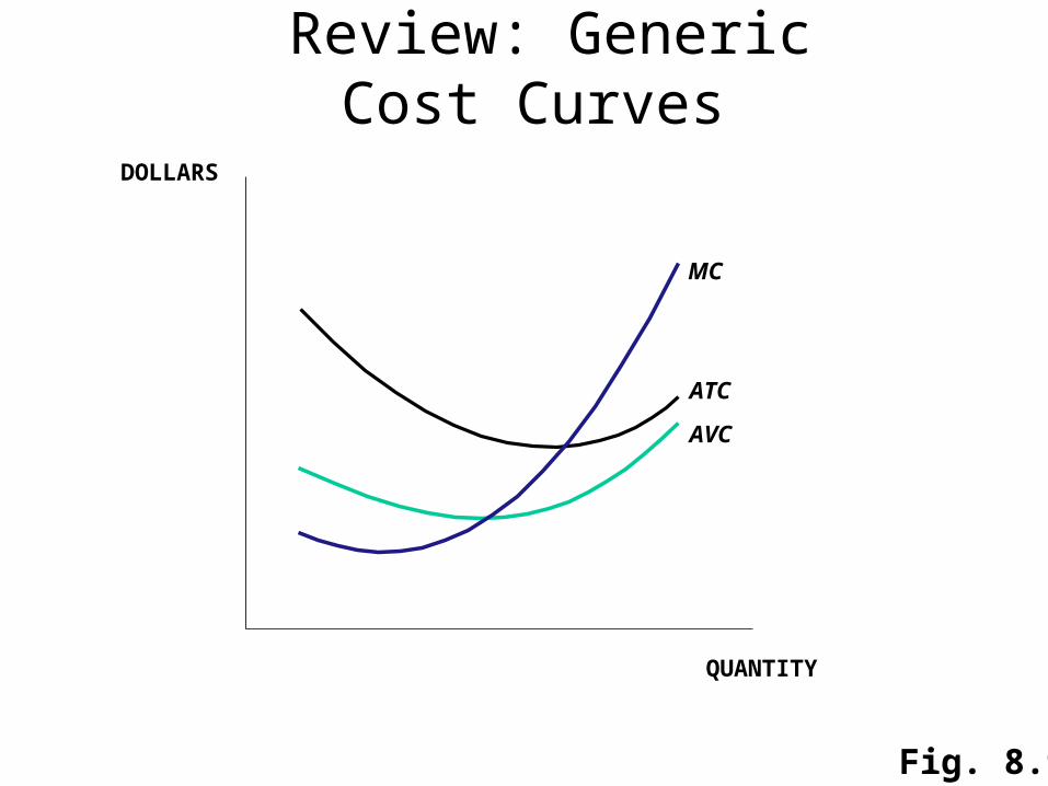
08_05

DOLLARS

QUANTITY

MC

ATC

AVC

Fig. 8.9

Review: Generic Cost Curves

Review: Profit Maximization06_08

Total costs

100

100

200

100

300

400

1 2 3 4 50

1 2 3 4 50

QUANTITY PRODUCED

QUANTITY PRODUCED

DOLLARS

Total revenue

Profits

DOLLARS

Fig 6.8

Profit Max Rule: MR=MC

08_05

DOLLARS

QUANTITY

MC

ATC

AVC

Fig. 8.9

Zero Economic Profit(P = MC = ATC)

P2

Break Even Point

Fig. 8.9

Negative Economic Profits (AVC<P<ATC)

P3

08_05

DOLLARS

QUANTITY

MC

ATC

AVC

Negative Profits

Q2

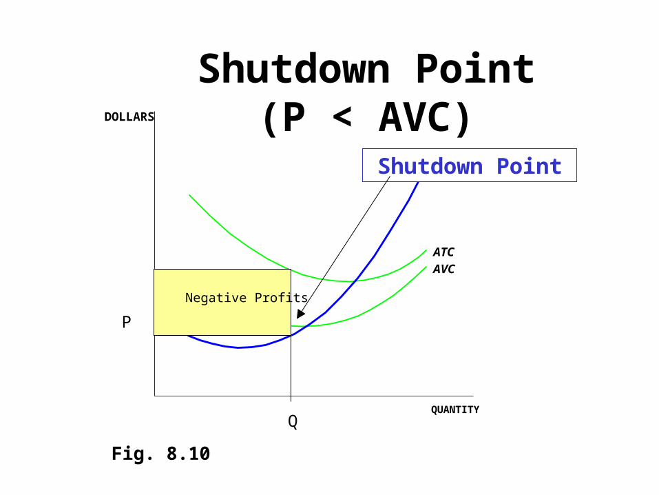
08_05

DOLLARS

QUANTITY

MC

ATC

AVC

Fig. 8.10

Shutdown Point(P < AVC)

P

Negative Profits

Q

Shutdown Point

Measuring Efficiency

• Consumer Surplus + Producer Surplus= Total Social Profit

• Deadweight Loss: The loss in total social profit due to an inefficient level of production.

• Examples: Taxes and Price Controls

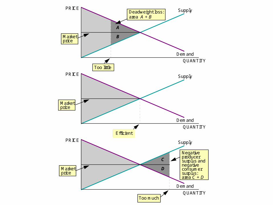
07_07

Too little

Efficient

QUANTITY

PRICE

Too much

Demand

Supply

C

D

Negative producer surplus and negative consumer surplus: area C + D

QUANTITY

PRICE

Demand

Supply

A

B

QUANTITY

PRICE

Demand

Supply

Deadweight loss: area A + B

Market price

Market price

Market price

Taxation and Deadweight Loss

07_08A

Old supply curve

Demand curve

QUANTITY

PRICE

Deadweight Loss from a Sales Tax

New supply curve

S shifts up by amount of tax

P* Tax RevDWL

CS

PSPp

Pc

Qt Q*

Quantity

MC = S

ATC

Pri

ce o

r C

ost (

$)

q0

S0

D0

Q0P

rice

($)

Quantity

P0 P0

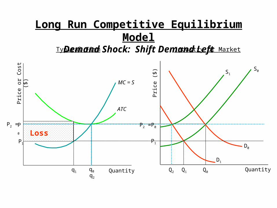
Typical Firm Industry or Market

Short Run Equilbrium

Firm: P0 = MR = MC

Industry: Qd = Qs @ P0

Long Run Equilbrium

Firm: Econ = 0

Industry: Firms @ Min LRATC

Long Run EquilibriumCondtions

(1) Many small firms Homogenous product.

(2) Identical product

(3) Perfect Information. Total Knowledge

(4) Free entry and exit.

Results Price taker with no market power. Firm believes it can sell it all

if it takes market price.

Always P=MR=MC @ min ATC

Perfectly Competitive MarketAssumptions

Quantity

MC = S

ATC

Pri

ce o

r C

ost (

$)

q0

S0

D0

Q0

Pri

ce (

$)

Quantity

Typical Firm Industry or Market

D1

Q1

P1P1

q1

S1

Long Run Competitive Equilibrium ModelDemand Shock: Shift Demand Left

Loss

Q2q2

P0P2 = P2 = P0

Quantity

MC = S

ATC

Pri

ce o

r C

ost (

$)

q0

S0

D0

Q0

Pri

ce (

$)

Quantity

Typical Firm Industry or Market

D1

Q1

P1P1

q1

S1

Q2q2

P0 P0P2 = P2 =

Long Run Competitive Equilibrium ModelDemand Shock: Shift Demand Right

Profits

Lesson 15 Monopoly: Part 1

What is a Monopoly?

• Many small firms

• Homogeneous Good

• Perfect Information• No Barriers to Entry or

Exit

• Small Output Compared to Industry

• Price taker

• No market power

• Is effiecient

• 1 firm • Unique product• Perfect knowledge that

firm has you• Barriers to Entry or

Exit--Blocked• Price Setter• Extreme market power• Is inefficient

Competitive Firm Monopoly

What is the Profit Maximizing Rule

10_05

Total costs

Total costs

Total revenue

Total revenue

Maximum

Maximum

QUANTITY

DOLLARS

Slope equals price.

Slope equals marginal cost.

QUANTITY

DOLLARS

Competitive Firm

Monopoly

Slope equals marginal revenue.

Slope equals marginal cost.

MR=MC

TR = P * Q

= TR - TC

TC = ATC * QQuantity

MC

ATC

Pri

ce o

r C

ost (

$)

Monopoly

DMR

QM

PM

Model of a MonopolyPositive Economic Profits

TC = ATC * Q

TR = P * QQuantity

MC

ATCPri

ce o

r C

ost (

$)

Monopoly

QM

PM

= TR - TC

DMR

Model of a MonopolyNegative Economic Profits

Model of a Monopoly Board Problem

Market: Cadet Comforters Scenario: QD = 40 - P where Q: comforters / week

TC = Q2 + 4Q + 58 P: $ / comforter

Question: (a) Calulate the MR and MC functions.

(b) Depict the following curves on a graph: D, MR, MC.

(c) Determine the equilibrium price and quantity if the firm acts like a perfectly competitive firm. Depict PPC and QPC on the graph. Calculate the firm’s profits.

(d) Determine the equilibrium price and quantity if the firm acts like a monopoly. Depict PM and QM on the graph. Calculate the firm’s profits.

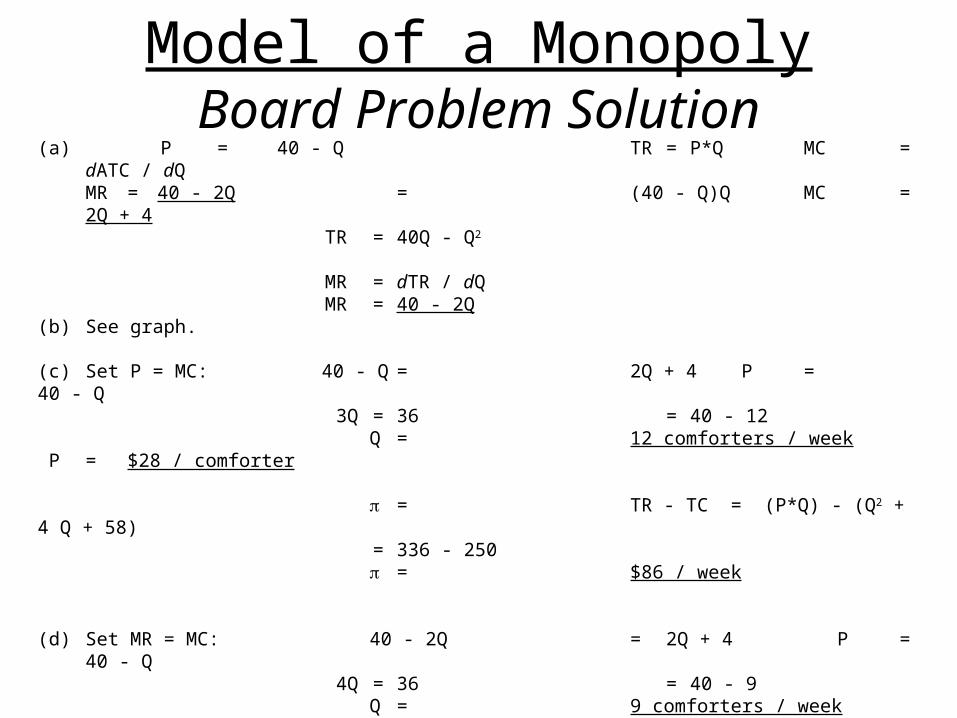
Model of a MonopolyBoard Problem Solution

(a) P = 40 - Q TR = P*Q MC = dATC / dQMR = 40 - 2Q = (40 - Q)Q MC = 2Q + 4

TR = 40Q - Q2

MR = dTR / dQMR = 40 - 2Q

(b) See graph.

(c) Set P = MC: 40 - Q = 2Q + 4 P = 40 - Q 3Q = 36 = 40 - 12 Q = 12 comforters / week P = $28 / comforter

= TR - TC = (P*Q) - (Q2 + 4 Q + 58)= 336 - 250

= $86 / week

(d) Set MR = MC: 40 - 2Q = 2Q + 4 P = 40 - Q 4Q = 36 = 40 - 9 Q = 9 comforters / week P = $31 / comforter

= TR - TC = (P*Q) - (Q2 + 4 Q + 58)= 279 - 175

= $104 / week

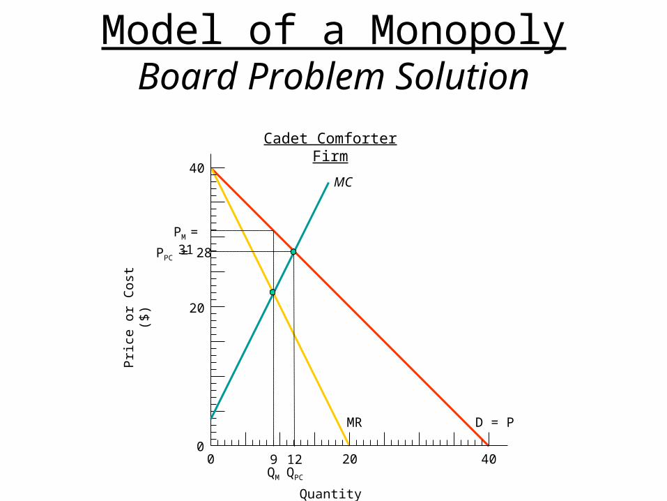
Model of a MonopolyBoard Problem Solution

Quantity

Pri

ce o

r C

ost (

$)Cadet Comforter Firm

D = PMR

MC

PPC = 28

PM = 31

20 4000

20

40

QM

9QPC

12

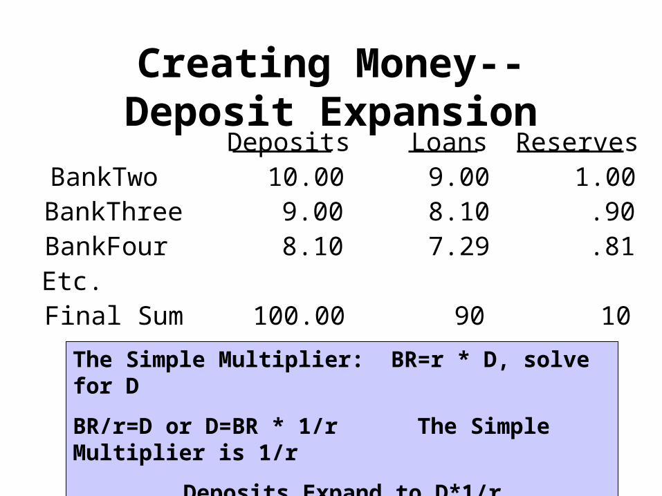
Creating Money--Deposit ExpansionDeposits Loans Reserves

BankTwo 10.00 9.00 1.00BankThree 9.00 8.10 .90BankFour 8.10 7.29 .81Etc.Final Sum 100.00 90 10

The Simple Multiplier: BR=r * D, solve for D

BR/r=D or D=BR * 1/r The Simple Multiplier is 1/r

Deposits Expand to D*1/r

Deriving The Money Multiplier

• MB=CU+BR which the Fed controls

• We know that M=CU + D

• Substitute in CU=kD and we get

• M=kD+D or M= (k+1)D

• We also know that BR=r*D and that MB=CU+BR

• Substitute in and MB=kD+rD or MB=(k+r)D

• To find the link divide M by MB: (k+1)D/(k+r)D The Money Multiplier = (k+1)/(k+r)

The multiple by which the money supply changes due to a change in the monetary base.

Lesson 27: Investment in New Capital

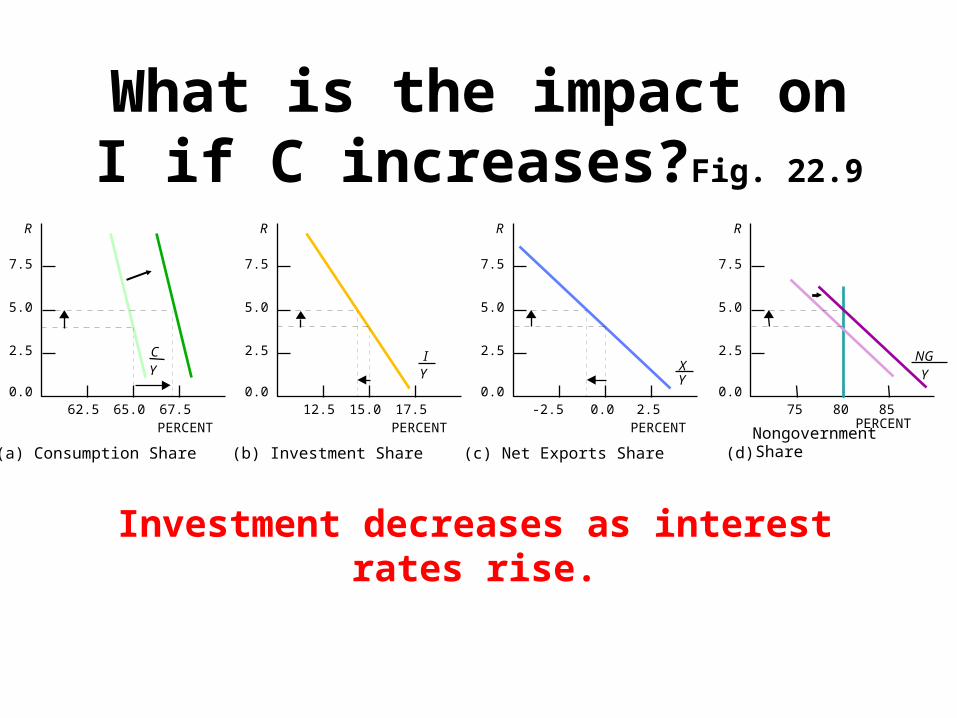
What is the impact on I if C increases?Fig. 22.9

22_09R

2.5

5.0

7.5

0.065.062.5 67.5

C Y

(a) Consumption Share

R

2.5

5.0

7.5

0.015.012.5 17.5

I Y

(b) Investment Share

R

2.5

5.0

7.5

0.08075 85

R

2.5

5.0

7.5

0.00.0 2.5

XY

(c) Net Exports Share

-2.5PERCENT PERCENT PERCENT PERCENT

NG Y

(d)NongovernmentShare

Investment decreases as interest rates rise.

“We figure it was HERE when the recession officially began.”

Taylor p. 677

Lesson 31 Aggregate Expenditure

The Rounds of the Multiplier Process fig 26.2

26_02

BILLIONS OF

DOLLARS

111 102 93 6 854 7

300

250

200

150

100

50

0

$250 billion

ROUNDMPC = .6

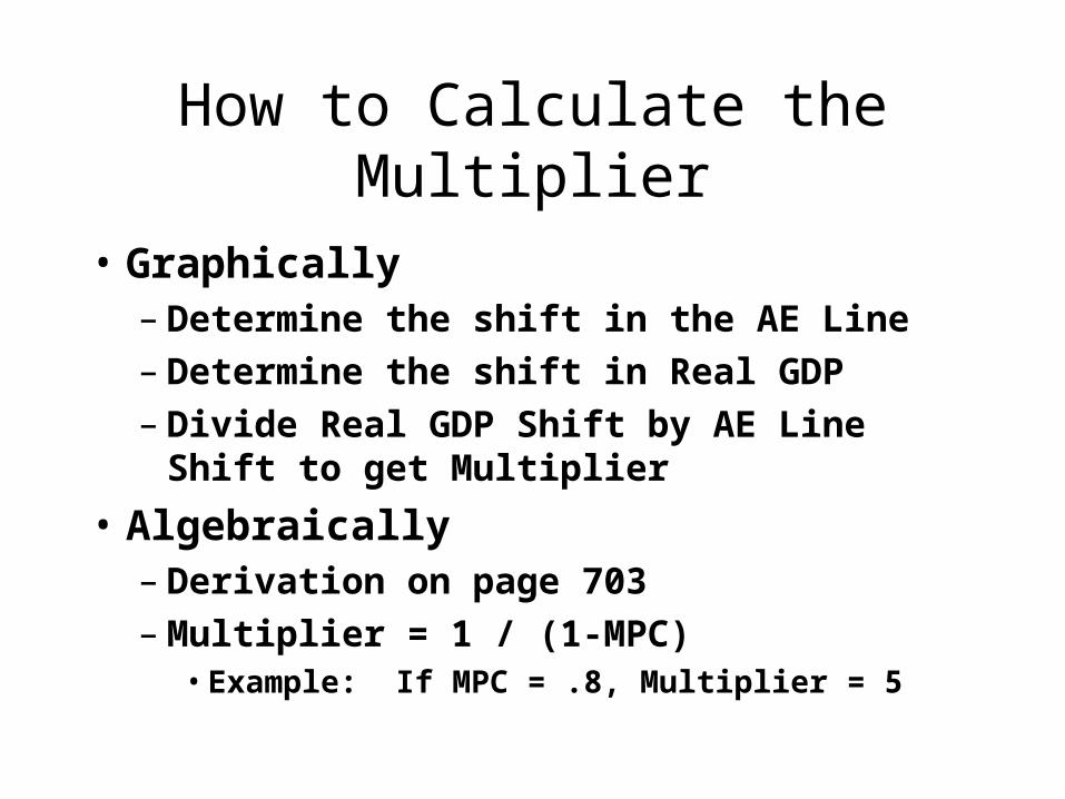
• Graphically– Determine the shift in the AE Line– Determine the shift in Real GDP– Divide Real GDP Shift by AE Line Shift to get

Multiplier

• Algebraically– Derivation on page 703– Multiplier = 1 / (1-MPC)

• Example: If MPC = .8, Multiplier = 5

How to Calculate the Multiplier

45 line

BoomAE line

e

c

d

NormalAE line

RecessionAE line

INCOME OR REAL GDP

(TRILLIONS OF 1992 DOLLARS)

5.75 6.506.256.00

6.50

SPENDING(TRILLIONS OF 1992 DOLLARS)

6.25

6.00

5.75

25_11B

SPENDING

(TRILLIONS

OF 1992 DOLLARS

d

6.25

6.50

6.00

5.75

Year 1 Year 3Year 2

c

e

b

a

(Boom)

(Real GDP=potential GDP)

(Recession)

Spending BalanceRecessions and Booms fig. 25.11