T

T

2

2

22

2 1ty

vxy

maF

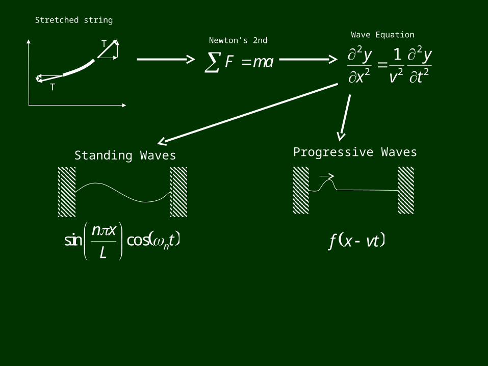
Standing Waves Progressive Waves

tL

xnn

cossin

vtxf

Stretched string

Newton’s 2ndWave Equation

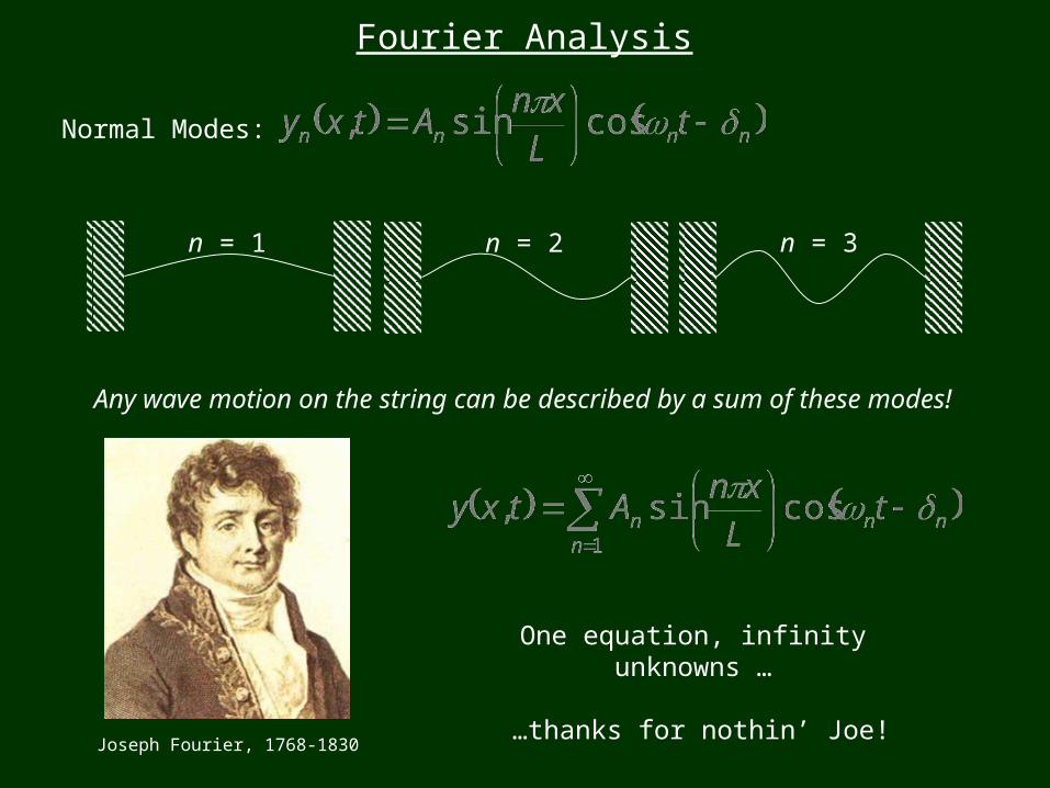
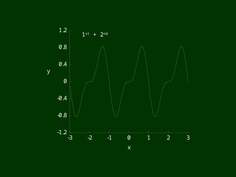
Any wave motion on the string can be described by a sum of these modes!

Fourier Analysis

Normal Modes:

n = 1 n = 2 n = 3

Joseph Fourier, 1768-1830

One equation, infinity unknowns …

…thanks for nothin’ Joe!

1

sinn

n Lxn

Bxy

Focus on the shape first! y(x)

How to find a specific Bn?

L

nn

L

dxL

xnL

xnBdx

Lxn

xy0 1

*

0

*

sinsinsin

coscossinsin 21

dx

Lxnn

LxnnB

n

Ln

1 0

**

coscos2

This reduces series to 1 term!

Mathematically…

Multiply by nth harmonic and integrate.

L

n

n

Lxnn

nnL

Lxnn

nnLB

01

*

*

*

* sinsin2

1

**

** 00sinsin

2n

n nnnnL

nnnnLB

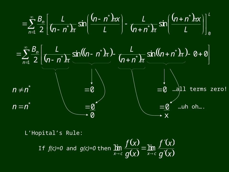
*nn

*nn

0 0 …all terms zero!

…uh oh….0 00

xgxf

xgxf

cxcx

limlim

L’Hopital’s Rule:

If f(c)=0 and g(c)=0 then

x

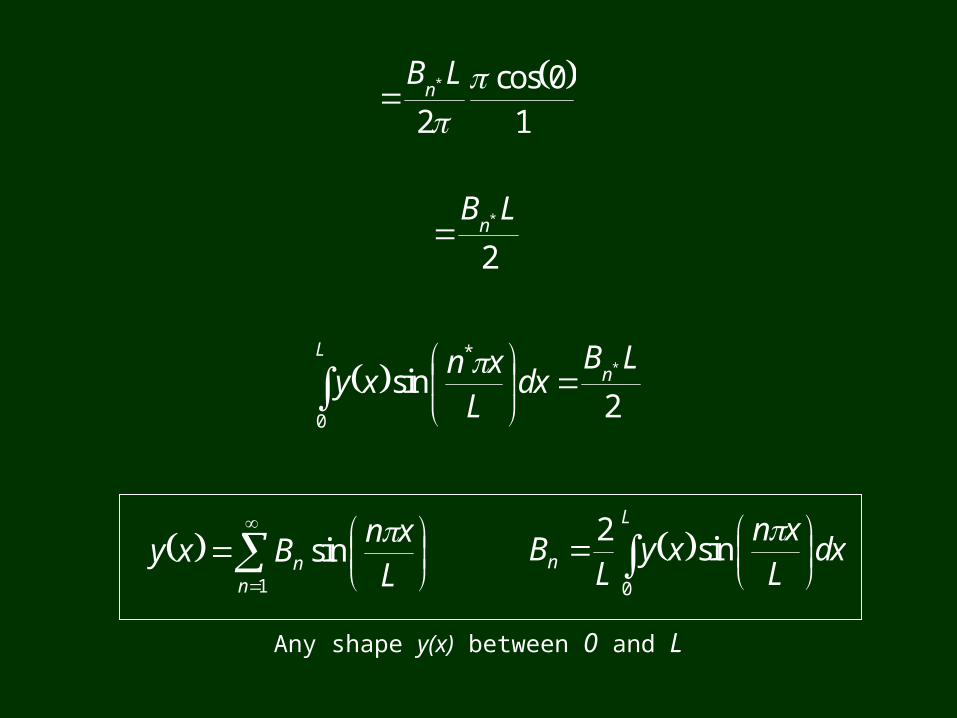
10cos

2

* LB

n

2

*LBn

2

sin*

0

* LBdx

Lxn

xy nL

dxL

xnxy

LB

L

n

0

sin2

1

sinn

n Lxn

Bxy

Any shape y(x) between 0 and L

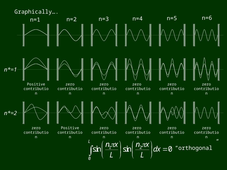
n=1 n=2 n=3 n=4 n=5 n=6

Positive contribution

zero contribution

zero contribution

zero contribution

zero contribution

zero contribution

zero contribution

Positive contribution

zero contribution

zero contribution

zero contribution

zero contribution

Graphically….

0sinsin0

21

L

dxL

xnL

xn “orthogonal”

n*=1

n*=2

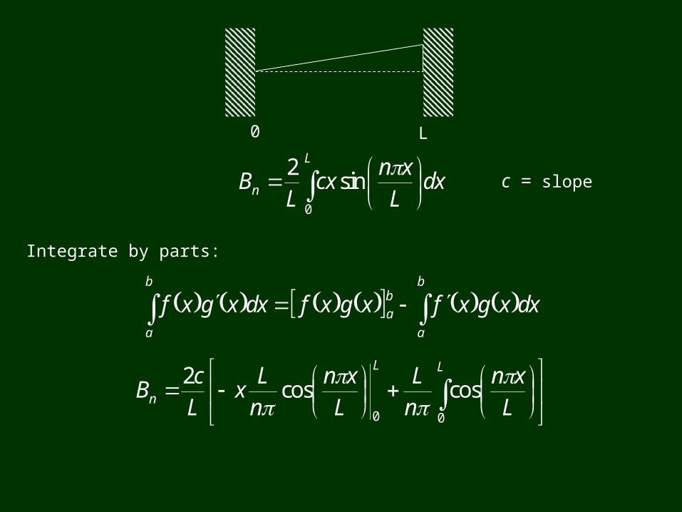
0 L

dxL

xncx

LB

L

n

0

sin2

Integrate by parts:

b

a

ba

b

a

dxxgxfxgxfdxxgxf

LL

n Lxn

nL

Lxn

nL

xLc

B00

coscos2

c = slope

LL

n Lxn

nL

Lxn

nL

xLc

B00

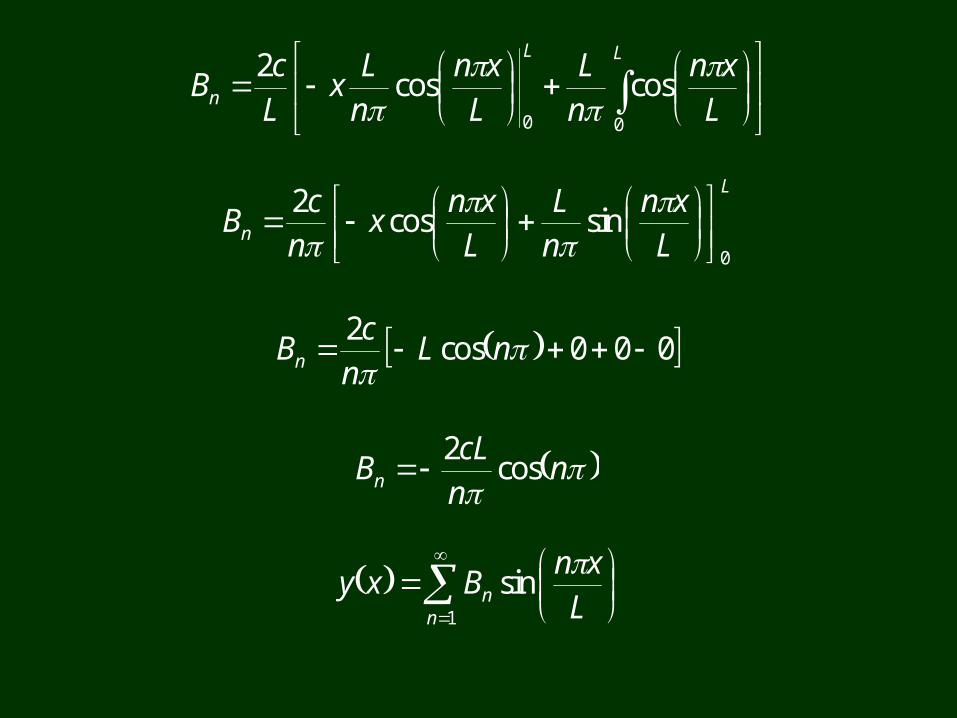
coscos2

L

n Lxn

nL

Lxn

xn

cB

0

sincos2

000cos2

nLn

cBn

nncL

Bn cos2

1

sinn

n Lxn

Bxy

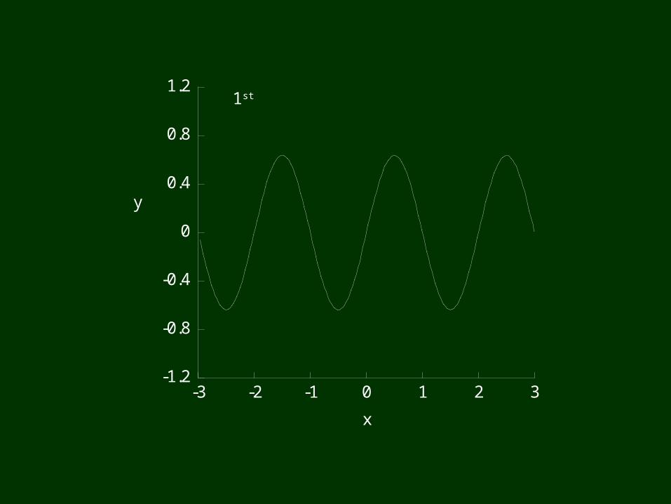
-1.2

-0.8

-0.4

0

0.4

0.8

1.2

-3 -2 -1 0 1 2 3

x

y

1st

-1.2

-0.8

-0.4

0

0.4

0.8

1.2

-3 -2 -1 0 1 2 3

x

y

1st + 2nd

-1.2

-0.8

-0.4

0

0.4

0.8

1.2

-3 -2 -1 0 1 2 3

x

y

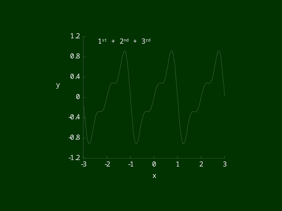
1st + 2nd + 3rd

-1.2

-0.8

-0.4

0

0.4

0.8

1.2

-3 -2 -1 0 1 2 3

x

y

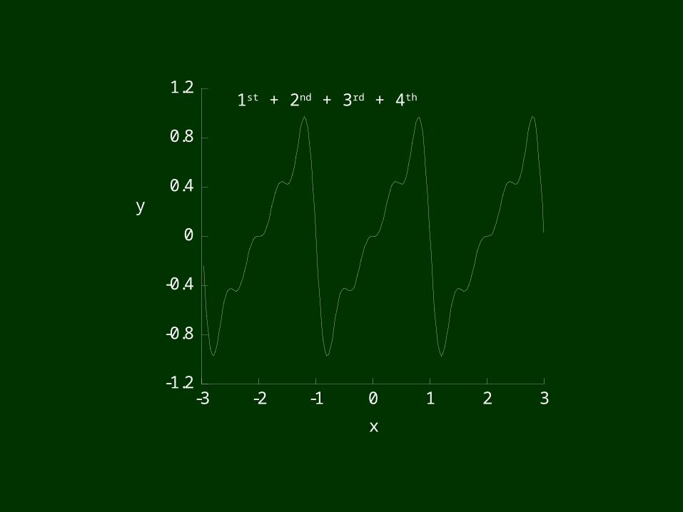
1st + 2nd + 3rd + 4th

-1.2

-0.8

-0.4

0

0.4

0.8

1.2

-3 -2 -1 0 1 2 3

x

y

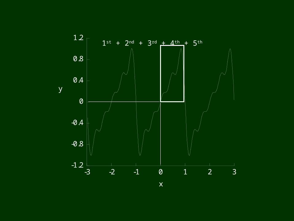
1st + 2nd + 3rd + 4th + 5th

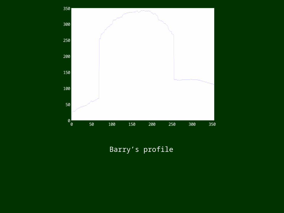
Barry’s profile

0 50 100 150 200 250 300 3500

50

100

150

200

250

300

350

Barry’s profile

0 50 100 150 200 250 300 350 4000

20

40

60

80

100

120

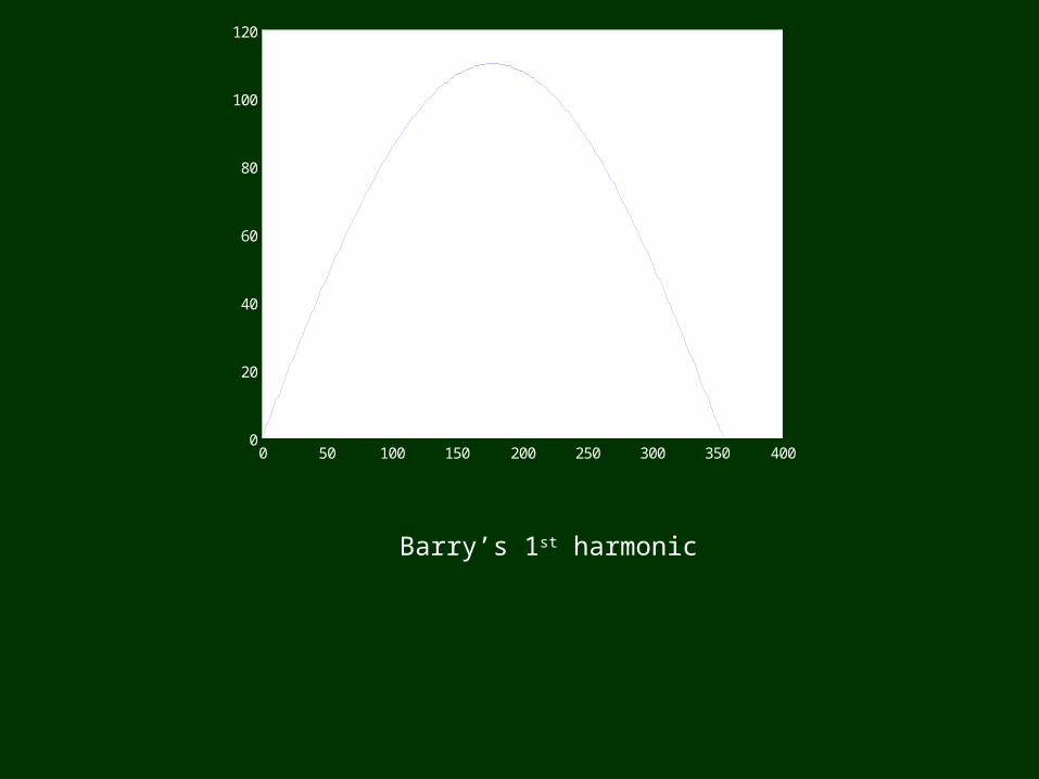
Barry’s 1st harmonic

0 50 100 150 200 250 300 350 4000

20

40

60

80

100

120

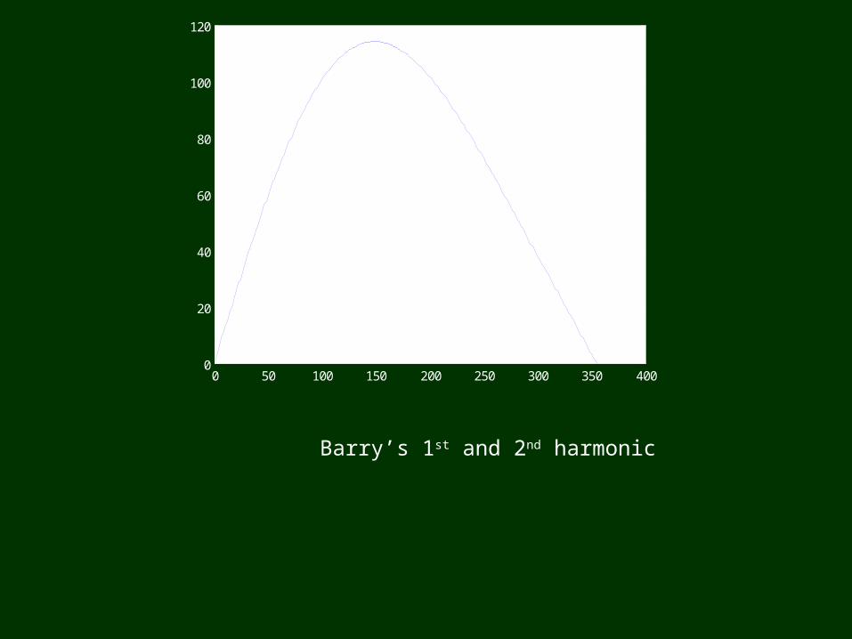
Barry’s 1st and 2nd harmonic

0 50 100 150 200 250 300 350 400-100

-50

0

50

100

150

200

250

Barry’s 1st, 2nd, and 3rd harmonic

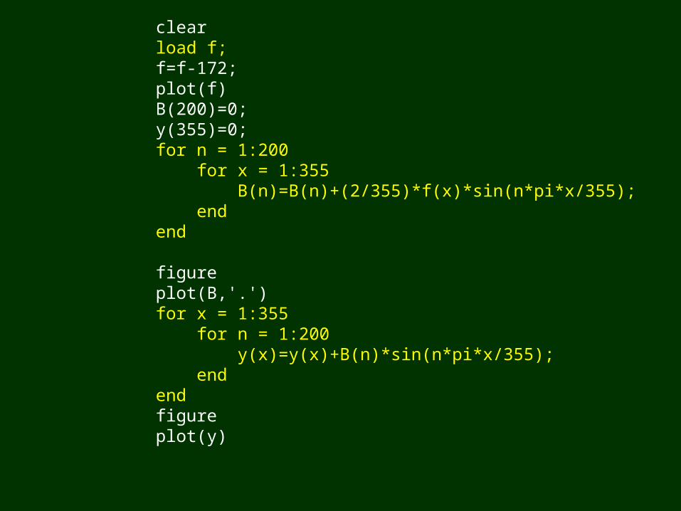
clearload f;f=f-172;plot(f)B(200)=0;y(355)=0;for n = 1:200 for x = 1:355 B(n)=B(n)+(2/355)*f(x)*sin(n*pi*x/355); endend

figureplot(B,'.')for x = 1:355 for n = 1:200 y(x)=y(x)+B(n)*sin(n*pi*x/355); endendfigureplot(y)

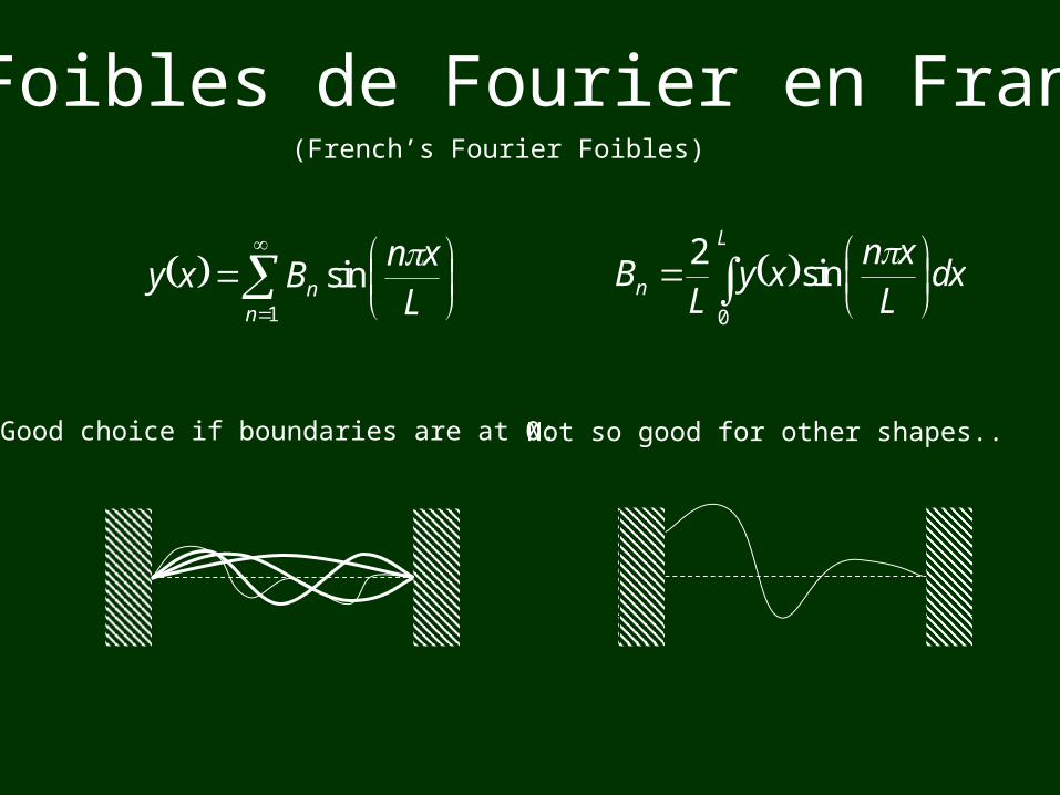
(French’s Fourier Foibles)

1

sinn

n Lxn

Bxy dx

Lxn

xyL

BL

n

0

sin2

Good choice if boundaries are at 0: Not so good for other shapes..

Les Foibles de Fourier en Frances

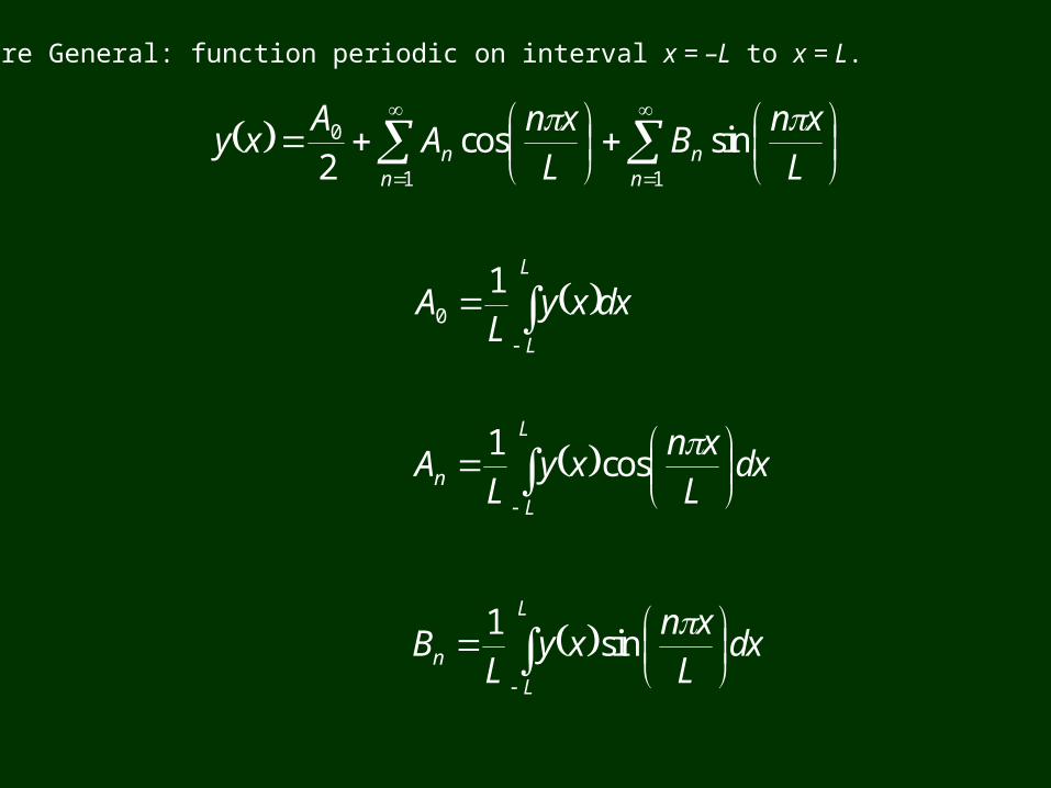
More General: function periodic on interval x = –L to x = L.

11

0 sincos2 n

nn

n Lxn

BL

xnA

Axy

dxL

xnxy

LB

L

L

n

sin1

dxL

xnxy

LA

L

L

n

cos1

dxxyL

AL

L

10

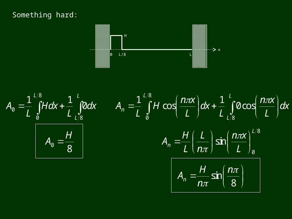
Something hard:

0 L/8 L

H

x

L

L

L

dxL

HdxL

A8

8

0

0 011

80

HA

L

L

L

n dxL

xnL

dxL

xnH

LA

8

8

0

cos01

cos1

8

0

sinL

n Lxn

nL

LH

A

8

sin

n

nH

An

0sin1

8

0

L

n dxL

xnH

LB

8

0

cosL

n Lxn

nL

LH

B

8

cos1

n

nH

Bn

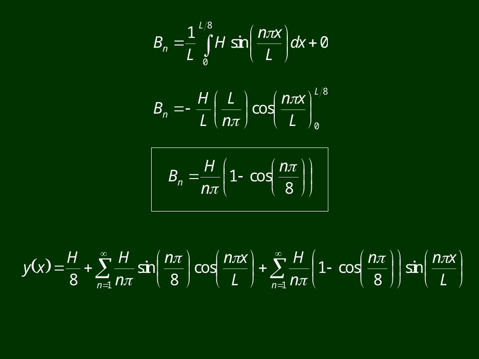
11

sin8

cos1cos8

sin8 nn L

xnnnH

Lxnn

nHH

xy

0 L

0

H

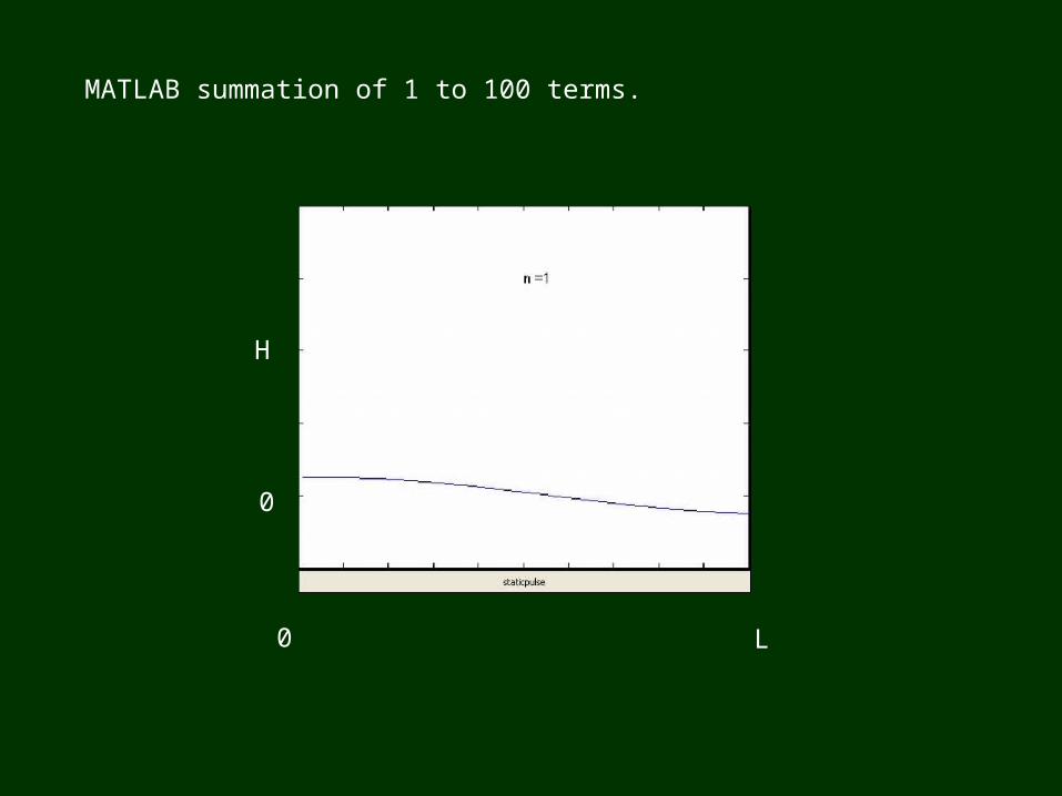
MATLAB summation of 1 to 100 terms.

Any well behaved repetitive function can be described as an infinite sum of sinusoids with variable amplitudes (a Fourier Series). On a stretched string these correspond to the normal modes. Fourier analysis can describe arbitrary string shapes as well as progressive waves and pulses.