t rivello readings ch. 13 - mit opencourseware · materials and structures. le t ’s first...
TRANSCRIPT

MIT - 16.20 Fall, 2002
Unit 9 Effects of the Environment
Readings: Rivello 3.6, 3.7 T & G Ch. 13 (as background), sec. 154
specifically
Paul A. Lagace, Ph.D.Professor of Aeronautics & Astronautics
and Engineering Systems
Paul A. Lagace © 2001

MIT - 16.20 Fall, 2002
Thus far we have discussed mechanical loading and the stresses and strains caused by that. We noted, however, that the environment can have an effect on the behavior of materials and structures. Let’s first consider:
Temperature and Its Effects
2 basic effects:
• expansion / contraction
• change of material properties
Look, first, at the former:
Concept of Thermal Stresses and Strains
Materials and structures expand and contract as the temperature changes. Thus:
εT = α (∆ T)
thermal temperature change
strain coefficient of thermal expansion (C.T.E.) units: 1
degrees
Paul A. Lagace © 2001 Unit 9 - p. 2

MIT - 16.20 Fall, 2002
If these thermal expansions / contractions are resisted by some means, then “thermal stresses” can arise. However, “thermal stresses” is a misnomer, they are really…
“stresses due to thermal effects” -- stresses are always “mechanical”
(we’ll see this via an example)
--> Consider a 3-D generic material. Then we can write:
T −εij = α ij ∆T (9 1)
i, j = 1, 2, 3 (as before)
αij = 2nd order tensor
The total strain of a material is the sum of the mechanical strain and the thermal strain.
mechanical thermal
M T −εij = εij + εij (9 2)
total Paul A. Lagace © 2001 Unit 9 - p. 3

MIT - 16.20 Fall, 2002
• (“actual”) total strain (εij): that which you actually measure; the physical deformation of the part
T • thermal strain ( εij ): directly caused by temperature differences M
• mechanical strain (εij ): that part of the strain which is directly
related to the stress
Relation of mechanical strain to stress is: Mεij = Sijkl σkl
compliance
Substituting this in the expression for total strain (equation 9-2) and using the expression for thermal strain (equation 9-1), we get:
εij = Sijkl σkl + α ij ∆ T
⇒ Sijkl σkl = εij − α ij ∆ T
We can multiply both sides by the inverse of the compliance…that is merely the elasticities:
−1 S
ijkl = Eijkl
Paul A. Lagace © 2001 Unit 9 - p. 4

MIT - 16.20 Fall, 2002
⇒ σkl = Eijkl εij − Eijkl αij ∆T
This is the same equation as we had before except we have the thermal terms:
Eijkl αij ∆ T
--> so how does a “thermal stress” arise?
Consider this example:
If you have a steel bar lying on a table and heat it, it will expand. Since it is unconstrained it expands freely and no stresses occur. That is, the thermal strain is equal to the total strain. Thus, the mechanical strain is zero and thus the “thermal stress” is zero.
Figure 9.1 Free thermal expansion of a steel bar
Paul A. Lagace © 2001 Unit 9 - p. 5

MIT - 16.20 Fall, 2002
--> However, if the bar is constrained, say at both ends:
Figure 9.2 Representation of constrained steel bar
Then, as it is heated, the rod cannot lengthen. The thermal strain is the same as in the previous case but now the total strain is zero (i.e., no physical deformation).
Starting with (in one direction):
ε = εM + εT
with: ε = 0
Thus, the mechanical strain is the negative of the thermal strain.
Paul A. Lagace © 2001 Unit 9 - p. 6

εεε
MIT - 16.20 Fall, 2002
Stresses will arise due to the mechanical strain and these are the so-called “thermal stresses”.
Due to equilibrium there must be a reaction at the boundaries.
(must always have ∫ σdA = Force for equilibrium)
Think of this as a two-step process…
Figure 9.3 Representation of stresses due to thermal expansion as two-step process
expands due to ∆∆∆∆T, εεεεT
Reaction force of boundaries related to mechanical strain, εM
εM = -εT
⇒ εtotal = 0 (no physical deformation)
Paul A. Lagace © 2001 Unit 9 - p. 7

MIT - 16.20 Fall, 2002
Values of C.T.E.’s
Note: αij = αji
• Anisotropic Materials
6 possibilities: α11, α22, α33, α12, α13, α23
⇒ ∆T can cause shear strains
not true in “engineering” materials • Orthotropic Materials
3 possibilities: α11, α22, α33
⇒ ∆T only causes extensional strains
Notes: 1. Generally we deal with planar structures and are interested only in α11 and α22
2. If we deal with the material in other than the principal material axes, we can “have” an α12
Transformation obeys same law as strain (it’s a tensor).
Paul A. Lagace © 2001 Unit 9 - p. 8

MIT - 16.20 Fall, 2002
2-D form:
α αβ = l lβγασγασ ˜˜
∗ ∗ α11, α22 (in - plane values) ∗ α12 = 0 (in material axes)
3-D form:
αij = l lj lαkli k
So, in describing deformation in some axis system at an angle θ to the principal material axes…..
Figure 9.4 Representation of 2-D axis transformation ~ y2
y1 ~θ
y2
θ + CCW
y1 Paul A. Lagace © 2001 Unit 9 - p. 9

MIT - 16.20 Fall, 2002
∗ α 11 = cos2 θ α11 + sin2 θ α∗ 22
∗ α 22 = sin2θ α11 + cos2θ α∗ 22
∗ ∗ α 12 = cos θ sinθ (α22 − α11) ∗ ∗only exists if α11 ≠ α22
[isotropic ⇒ no shear]
• Isotropic Materials
1 value: α is the same in all directions
Typical Values for Materials:
Units: x 10-6/°F
µin/in/°F
strain/°F
⇒ µstrain/°F
Paul A. Lagace © 2001 Unit 9 - p. 10
Material C.T.E.
Uni Gr/Ep (perpendicular to fibers)
Uni Gr/Ep (along fibers)
Titanium
Aluminum
Steel
16
-0.2
5
12.5
6

MIT - 16.20 Fall, 2002
Notes:
• Graphite/epoxy has a negative C.T.E. in the fiber direction so it contracts when heated
Implication: by laying up plies with various orientation can achieve a structure with a C.T.E. equal to zero in a desired direction
• C.T.E. of a structure depends on C.T.E. and elastic constants of the parts
E = E
E = 0 (perfectly compliant)
1
C.T.E. = 5
2 examples
1) total α of
C.T.E. = 2 structure = 5
E = E1
C.T.E. = 5 2) total α of
C.T.E. = 2 structure
E = ∞ (perfectly rigid) = 2
Paul A. Lagace © 2001 Unit 9 - p. 11

MIT - 16.20 Fall, 2002
• α = α(T) ⇒ C.T.E. is a function of temperature (see MIL HDBK 5 for metals). Can be large difference.
Implication: a zero C.T.E. structure may not truly be attainable since it may be C.T.E. at T1 but not at T2 !
--> Sources of temperature differential (heating)
• ambient environment (engine, polar environment, earth shadow, tropics, etc.)
• aerodynamic heating • radiation (black-body)
--> Constant ∆T (with respect to spatial locations)
In many cases, we are interested in a case where ∆T (from some reference temperature) is constant through-the-thickness, etc.
• thin structures • structures in ambient environment for long periods of time
Relatively easy problem to solve. Use: • equations of elasticity • equilibrium • stress-strain
Paul A. Lagace © 2001 Unit 9 - p. 12
MIT - 16.20 Fall, 2002
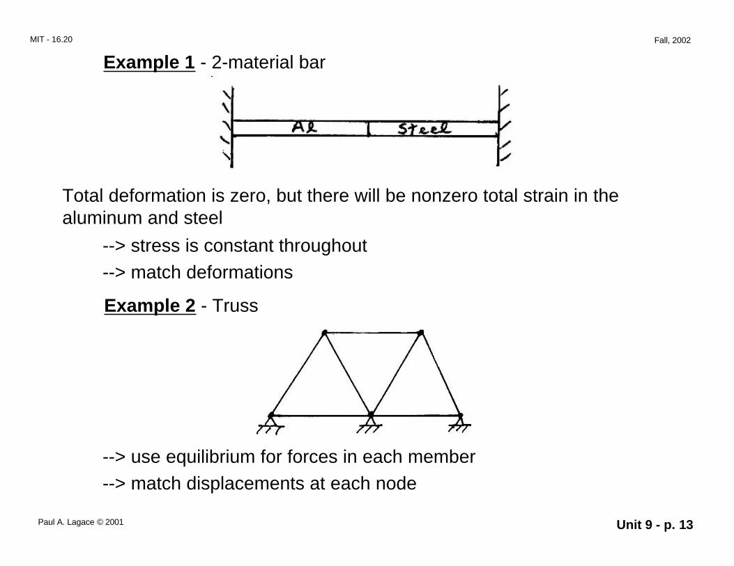
Example 1 - 2-material bar
Total deformation is zero, but there will be nonzero total strain in the aluminum and steel
--> stress is constant throughout
--> match deformations
Example 2 - Truss
--> use equilibrium for forces in each member
--> match displacements at each node
Paul A. Lagace © 2001 Unit 9 - p. 13

MIT - 16.20 Fall, 2002
Example 3 - bimetallic strip
Each metal has different α’s. What will happen?
Bending!
--> Concept of self-equilibrating stresses
Must always be in equilibrium. General equation is:
∫ σdA = F where: F = externally applied force
If F = 0, can we still have stresses?
Yes, but they must be “self-equilibrating” (satisfy equilibrium in and of themselves):
∫ σdA = 0 This is the case of free expansion (thermal) of structures with varying properties or spatially-varying ∆T (we’ll address this in a bit)
Paul A. Lagace © 2001 Unit 9 - p. 14

MIT - 16.20 Fall, 2002
If α1 > α2 and ∆T > 0
T Tεij > εij1 2
(we’ll see more about this bending later)
Bimetallic strip used as temperature sensors!
--> ∆T varies spatially (and possibly with time as well, we analyze at any constant in time)
Must determine ∆T by looking at heat flux into structure. Three basic methods:
• induction
• convection
• radiation
Paul A. Lagace © 2001 Unit 9 - p. 15

MIT - 16.20 Fall, 2002
Convection most important in aircraft:
Aerodynamic Heating
look at adiabatic wall temperature
2 TAW = 1 + γ − 1
r M∞ T∞2 where:
γ = specific heat ratio (1.4 for air) r = "recovery factor" (0.8 - 0.9) M∞ = Mach number T∞ = ambient temperature (°K)
TAW is maximum temperature obtained on surface (for zero heat flux)
Note: @40,000 ft. M = 2 ⇒ TAW = 230°F
M = 3 ⇒ TAW = 600°F
⇒ (much above M = 2, cannot use aluminum since properties are too degraded)
worse in reentry
Paul A. Lagace © 2001 Unit 9 - p. 16

MIT - 16.20 Fall, 2002
Source of heat here is from air boundary layer: q = h (TAW - Ts)
surface temperature of bodyheat flux
heat transfer [watts/M2] coefficient
(convective constant)
(h is determined from boundary layer theory)
Radiation
Always important but especially in space (or at high temperature in atmosphere).
--> 2 considerations
1. Emissivity
--> surface emits heat
Paul A. Lagace © 2001 Unit 9 - p. 17

MIT - 16.20 Fall, 2002
q = - ε σ Ts4
surface temperature heat flux Stefan-Boltzmann constant
emissivity (a material property)
2. Absorptivity
heat q = α Is λ
angle factor
flux intensity of source absorptivity (a material property)
Figure 9.5 Representation of heat flux impinging on structure
angle of structure
like the sun
Is (intensity of source) Paul A. Lagace © 2001 Unit 9 - p. 18

MIT - 16.20 Fall, 2002
Heat conduction
The general equation for heat conduction is:
∂T qi
T = − kijT
∂xj
where:
T = temperature [°K] T wattsqi = heat flux per unit area in i direction m2
T wattskij = thermal conductivity m K °
(material properties) TThe kij are second order tensors
Paul A. Lagace © 2001 Unit 9 - p. 19
MIT - 16.20 Fall, 2002
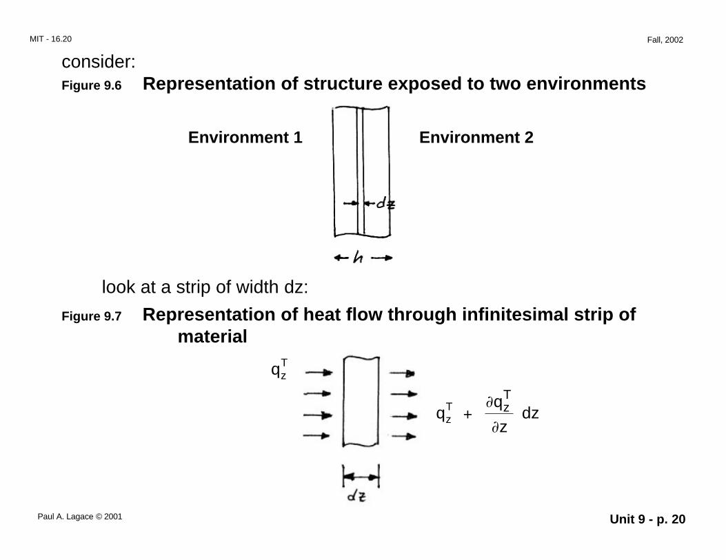
consider:Figure 9.6 Representation of structure exposed to two environments
Environment 1 Environment 2
look at a strip of width dz:
Figure 9.7 Representation of heat flow through infinitesimal strip of material
T qz
T T qz +
∂qz dz ∂z
Paul A. Lagace © 2001 Unit 9 - p. 20

MIT - 16.20 Fall, 2002
Do a balance of energy: T
qzT −
qz
T + ∂qz
dz = ρC ∂T dz
∂z ∂t
heat flux heat flux change in stored- = on side 1 on side 2 heat in strip
where: ρ = density C = specific heat capacity t = time
this becomes: T
−∂qz = ρC
∂T ∂z ∂t
Recalling that:
Tqz = − kT ∂T z ∂z
Paul A. Lagace © 2001 Unit 9 - p. 21

MIT - 16.20 Fall, 2002
we have:
∂ kz
T ∂T = ρC
∂T ∂z ∂z ∂t
If kzT and ρc are constant with respect to z (for one material they are),
then we get:
kT ∂2T ∂Tz = ρC ∂z2 ∂t
Fourier’s equation We call:
kT z = thermal diffusivity
ρC
More generally, for 3-D variation: ∂
kT ∂T
+ ∂ T ∂T ∂ T ∂T
= Cρ
∂T ∂x x ∂x ∂y
ky ∂y +
∂z kz ∂z ∂t
thermal conductivities in x, y, and z directions Paul A. Lagace © 2001 Unit 9 - p. 22
MIT - 16.20 Fall, 2002
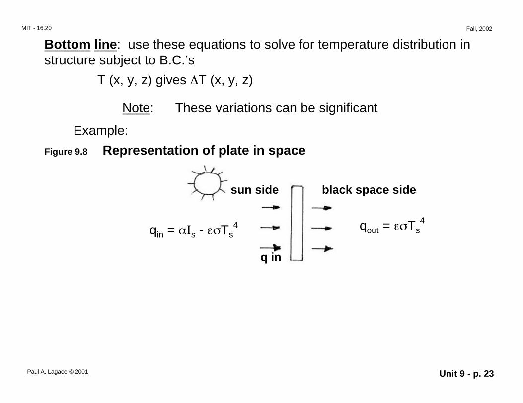
Bottom line: use these equations to solve for temperature distribution in structure subject to B.C.’s
T (x, y, z) gives ∆T (x, y, z)
Note: These variations can be significant
Example:
Figure 9.8 Representation of plate in space
4 qin
sun side black space side
q in
= αIs - εσTs 4 qout = εσTs
Paul A. Lagace © 2001 Unit 9 - p. 23

MIT - 16.20 Fall, 2002
could get other cases where T peaks in the center, etc.
Result:
⇒ Internal stresses (generally) arise if T varies spatially. (unless it is a linear variation which is unlikely given the governing equations).
Why?
consider an isotropic plate with ∆T varying only in the y-direction
Paul A. Lagace © 2001 Unit 9 - p. 24

∆∆∆
∆∆∆
MIT - 16.20 Fall, 2002
Figure 9.9 Representation of isotropic plate with symmetric y-variation of ∆T about x-axis
(for the time being, limit ∆T to be symmetric with respect to any of the axes)
Paul A. Lagace © 2001 Unit 9 - p. 25

MIT - 16.20 Fall, 2002
At first it would seem we get a deformation of a typical cross-section A-B as:
x
y
This basic shape would not vary in x. Note, however, that this deformation in the x-direction (u) varies in y.
∂u ⇒ ≠ 0
∂y
⇒ shear strain exists!
But, ∆T only causes extensional strains. Thus, this deformation cannot occur.
(in some sense, we have “plane sections must remain plane”)
Thus, the deformation must be:
Paul A. Lagace © 2001 Unit 9 - p. 26
MIT - 16.20 Fall, 2002
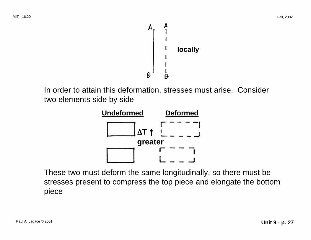
locally
In order to attain this deformation, stresses must arise. Consider two elements side by side
Undeformed Deformed
∆∆∆∆T ↑↑↑↑ greater
These two must deform the same longitudinally, so there must be stresses present to compress the top piece and elongate the bottom piece
Paul A. Lagace © 2001 Unit 9 - p. 27

MIT - 16.20 Fall, 2002
Thus:
εx = εx (x) εy = εy (y)
This physical argument shows we have thermal strains, mechanical strains and stresses.
self-equilibrating
a ∫−a
σydx = 0
b ∫−b
σxdy = 0
Causes
Paul A. Lagace © 2001 Unit 9 - p. 28

MIT - 16.20 Fall, 2002
Solution Technique
No different than any other elasticity problem. Use equations of elasticity subject to B. C.’s.
• exact solutions • stress functions
recall:
∇4φ = − Eα∇2 (∆T) − (1 − ν)∇2 V
• etc. (see Timoshenko)
--> Does this change for orthotropic materials?
NO (stress-strain equations change)
We’ve considered Thermal Strains and Stresses, now let’s look at the other effect:
Paul A. Lagace © 2001 Unit 9 - p. 29

MIT - 16.20 Fall, 2002
Degradation of Material Properties (due to thermal effects)
Here there are two major categories
1. “Static” Properties
• Modulus, yield stress, ultimate stress, etc. change with temperature (generally, T↑ ⇒ property ↓)
• Fracture behavior (fracture toughness) goes through a transition at “glass transition temperature”
ductile → brittle Tg
(see Rivello)
Paul A. Lagace © 2001 Unit 9 - p. 30

MIT - 16.20 Fall, 2002
Figure 9.10 Representation of variation of ultimate stress with temperature
Figure 9.11 Representation of change in stress-strain behavior with temperature
ductile as T increases) (generally, behavior is more
--> Thus, must use properties at appropriate temperature in analysis
MIL-HDBK-5 has much data Paul A. Lagace © 2001 Unit 9 - p. 31

MIT - 16.20 Fall, 2002
2. “Time-Dependent” Properties
There is a phenomenon (time-dependent) in materials known as creep. This becomes especially important at elevated temperature.
Figure 9.12 Representation of creep behavior
Hang a load P and monitor strain with time
resulting strain-time behavior
This keeps aluminum from being used in supersonic aircraft in critical areas for aerodynamic heating.
Paul A. Lagace © 2001 Unit 9 - p. 32

MIT - 16.20 Fall, 2002
“Other” Environmental Effects
• Temperature tends to be the dominating concern, but others may be important in both areas – atomic oxygen degrades properties – UV degrades properties – etc.
• Same effects may cause environmental strains like thermal strains:
Example - moisture Materials can absorb moisture. Characterized by a “swelling coefficient” = βij
Same “operator” as αij (C. T. E.) except it operates on moisture concentration, c:
sεij = βij c
“swelling” moisture concentration
strain swelling coefficient
Paul A. Lagace © 2001 Unit 9 - p. 33

MIT - 16.20 Fall, 2002
and then we have:
εij = εijM
+ εijT
+ εijS
total
This can be generalized such that the strain due to an environmental effect is:
environmental strain Eεij = χij X
environmentalenvironmental operator scalar
and the total strain is the sum of the mechanical strain(s) and the environmental strains
A strain of this “type” has become important in recent work. This deals with the field of
Paul A. Lagace © 2001 Unit 9 - p. 34
MIT - 16.20 Fall, 2002
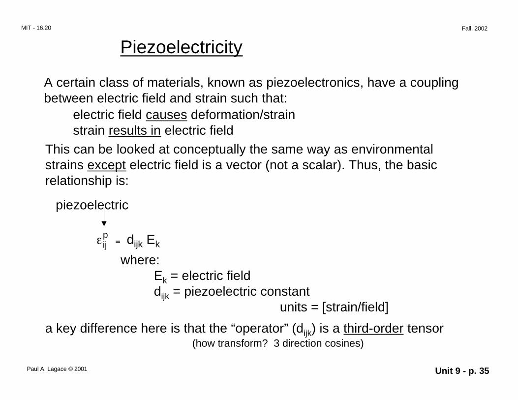
Piezoelectricity
A certain class of materials, known as piezoelectronics, have a coupling between electric field and strain such that:
electric field causes deformation/strain strain results in electric field
This can be looked at conceptually the same way as environmental strains except electric field is a vector (not a scalar). Thus, the basic relationship is:
piezoelectric
εijp
= d Ekijk
where: Ek = electric field dijk = piezoelectric constant
units = [strain/field]
a key difference here is that the “operator” (dijk) is a third-order tensor (how transform? 3 direction cosines)
Paul A. Lagace © 2001 Unit 9 - p. 35

MIT - 16.20 Fall, 2002
And we add this strain to the others to get the total strain
(consider the case with only mechanical and piezoelectric strain)
εij = εijM
+ εijp
Again, only the mechanical strain is related directly to the stress: εij = Sijmn σmn + dijk Ek
inverting gives:
σij = Eijmn εmn − Eijmn dmnk Ek
(watch the switching of indices!) thus we have “piezoelectric-induced” stresses of:
Eijmn dmnk Ek
if the piezoelectric expansion is physically resisted. Again, equilibrium (∫ σ = F) must be satisfied.
But, unlike environmental cases, the electric field is not just an external parameter from some uncoupled equation of state but there is a coupled equation:
Paul A. Lagace © 2001 Unit 9 - p. 36

MIT - 16.20 Fall, 2002
Di = eik Ek + dinm σmn note switch in indices since this is transpose of dielectric constant from previous equation
where:
eik = dielectric constant Di = electrical charge
--> “Normally”, when piezoelectric materials are utilized, “E-field control” is assumed. That is, E k is the independent variable and the electrical charge is allowed to “float” and take on whatever value results. But, when charge constraints are imposed the simultaneous set of equations:
σmn = Emnij εij − Emnij dijk Ek
Di = eik Ek + dinm σmn
must be solved. This is coupled with any other sources of strain (mechanical, etc.)
Paul A. Lagace © 2001 Unit 9 - p. 37
MIT - 16.20 Fall, 2002
Piezoelectrics useful for
• sensors • control of structures (particularly dynamic effects)
Note: electrical folk use a very different notation (e.g., S = strain)
Now that we’ve looked at the general “causes” of stress and strain and how to manipulate, etc., consider general structures and stress and strain in that context.
Paul A. Lagace © 2001 Unit 9 - p. 38