t -compilation for inference in probabilistic logic...
TRANSCRIPT
TP-Compilation for Inference in
Probabilistic Logic Programs
Jonas Vlasselaera, Guy Van den Broeckb, Angelika Kimmiga, WannesMeerta, Luc De Raedta
aKU Leuven, [email protected]
bUniversity of California, Los [email protected]
Abstract
We propose TP-compilation, a new inference technique for probabilistic logicprograms that is based on forward reasoning. TP-compilation proceeds incre-mentally in that it interleaves the knowledge compilation step for weightedmodel counting with forward reasoning on the logic program. This leads to anovel anytime algorithm that provides hard bounds on the inferred probabil-ities. The main difference with existing inference techniques for probabilisticlogic programs is that these are a sequence of isolated transformations. Typi-cally, these transformations include conversion of the ground program into anequivalent propositional formula and compilation of this formula into a moretractable target representation for weighted model counting. An empiricalevaluation shows that TP-compilation effectively handles larger instances ofcomplex or cyclic real-world problems than current sequential approaches,both for exact and anytime approximate inference. Furthermore, we showthat TP-compilation is conducive to inference in dynamic domains as it sup-ports efficient updates to the compiled model.
Keywords: Probabilistic Inference, Knowledge Compilation, ProbabilisticLogic Programs, Dynamic Relational Models
1. Introduction
During the last few years there has been a significant interest in com-bining relational structure with uncertainty. This has resulted in the fieldsof statistical relational learning (Getoor and Taskar, 2007; De Raedt et al.,
Preprint submitted to Elsevier June 7, 2016
2008), probabilistic programming (Pfeffer, 2014) and probabilistic databases(Suciu et al., 2011), which all address this combination. Probabilistic logicprogramming (PLP) languages such as PRISM (Sato, 1995), ICL (Poole,1993), ProbLog (De Raedt et al., 2007), LPADs (Vennekens et al., 2004) andCP-logic (Vennekens et al., 2009) form one stream of work in these fields.These formalisms extend the logic programming language Prolog with prob-abilistic choices on which facts are true or false. We refer to De Raedt andKimmig (2015) for a detailed overview.
A common task in PLP is to compute the probability of a set of queries,possibly given some observations. A recent insight is that probabilistic infer-ence for PLP corresponds to weighted model counting (WMC) on weightedlogical formulas (Fierens et al., 2015; Chavira and Darwiche, 2008; Darwiche,2009). As a result, state-of-the-art inference techniques rely on a three stepprocedure (Fierens et al., 2015): (1) transform the dependency structure ofthe logic program and the queries into a propositional formula, (2) com-pile this formula into a tractable target representation, and (3) compute theweighted model count (WMC). A recurring problem is that the first two stepsare computationally expensive, and infeasible for some real-world domains,especially if the domain is highly cyclic.
The key contribution of this paper is TP-compilation, a novel inferencetechnique for probabilistic logic programs that interleaves construction andcompilation of the propositional formula. TP-compilation uses the TcP op-erator that generalizes the TP operator (Van Emden and Kowalski, 1976)from logic programming to probabilistic logic programming. Whereas theTP operator finds one interpretation that satisfies the program, the TcP op-erator finds all possible interpretations and associated probabilities. At anypoint, after each application of the TcP operator, the WMC provides a lowerbound on the true probability of the queries and we thus realize an anytimealgorithm. We obtain an efficient realization of the TcP operator by repre-senting formulas as Sentential Decision Diagrams, which efficiently supportincremental formula construction and WMC (Darwiche, 2011).
The main advantage of TP-compilation is that forward reasoning allowsfor a natural way to handle cyclic dependencies. Because our approach doesnot require to convert the complete logic program into a propositional formulabefore compilation, no additional variables are introduced to break cycles.This considerably simplifies the compilation step and pushes the boundariesfor exact as well as approximate inference.
A second advantage is that constructing the formula incrementally results
2
in a set of formulas, rather than one big formula, which enables programupdates and inference in dynamic models, i.e., applications where time isinvolved. In case of program updates, clauses are added to or deleted from theprogram and TP-compilation can update the already compiled formulas. Thiscan cause significant savings compared to restarting inference from scratch.Dynamic models contain time explicitly, introducing a repeated structure inthe model. TP-compilation allows us to exploit this structure, as well as thegiven observations, to efficiently perform inference.
An empirical evaluation on real-world applications of biological and socialnetworks, web-page classification tasks and games demonstrates how ourapproach efficiently copes with cyclic and dynamic domains. We show thatTP-compilation outperforms state-of-the-art approaches on these problemswith respect to time, space and quality of results.
This paper extends the work of Vlasselaer et al. (2015) to stratified prob-abilistic logic programs with negation. Earlier work of Bogaerts and Van denBroeck (2015) extends the TcP operator towards general logic programs bymeans of approximation fixpoint theory, which is very general and powerful.When one is only interested in stratified logic programs, however, a muchsimpler result suffices, which we present here. Furthermore, we show howTP-compilation allows us to efficiently cope with dynamic models. This dy-namic approach is inspired by the work presented in Vlasselaer et al. (2016)but differs in two aspects. Firstly, we consider dynamic relational mod-els while Vlasselaer et al. (2016) consider dynamic Bayesian Networks, i.e.,models without cycles. Secondly, TP-compilation allows for a more flexi-ble approach that additionally exploits the observations to further scale upinference.
The paper is organized as follows. We start by reviewing the necessarybackground in Section 2. Sections 3 and 4 formally introduce the TcP opera-tor and corresponding algorithm. We deal with dynamic domains in Section 5and discuss experimental results in Section 6. Before concluding, we discussrelated work in Section 7.
2. Background
We review the basics of (probabilistic) logic programming. First, weintroduce definite clause programs and show how to include negation. Next,we discuss probabilistic logic inference and knowledge compilation.
3

2.1. Logical Inference for Definite Clause Programs
A term is a variable, a constant, or a functor applied on terms. Anatom is of the form p(t1, . . . , tm) where p is a predicate of arity m and theti are terms. A definite clause is a universally quantified expression of theform h :− b1, ..., bn where h and the bi are atoms and the comma denotesconjunction. The atom h is called the head of the clause and b1, ..., bn thebody. The meaning of such a clause is that whenever the body is true, thehead has to be true as well. A fact is a clause that has true as its body andis written more compactly as h. A definite clause program is a finite set ofdefinite clauses, also called rules. If an expression does not contain variablesit is ground.
Let A be the set of all ground atoms that can be constructed from theconstants, functors and predicates in a definite clause program P . A Her-brand interpretation of P is a truth value assignment to all a ∈ A, and isoften written as the subset of true atoms (with all others being false), or asa conjunction of atoms. A Herbrand interpretation satisfying all rules in theprogram P is a Herbrand model. The model-theoretic semantics of a definiteclause program is given by its unique least Herbrand model, that is, the setof all ground atoms a ∈ A that are entailed by the logic program, writtenP |= a.
Example 1. Consider the following definite clause program:
edge(b, a). edge(b, c).
edge(a, c). edge(c, a).
path(X, Y ) : - edge(X, Y ).
path(X, Y ) : - edge(X,Z), path(Z, Y ).
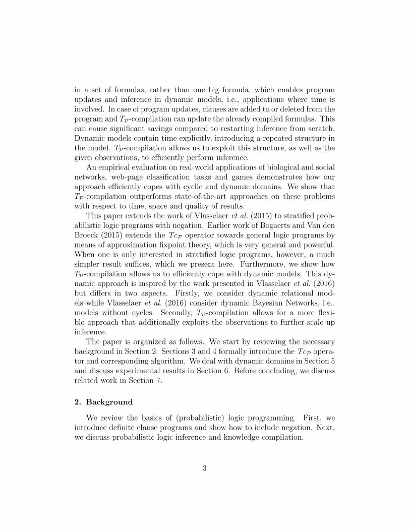
The facts represent the edges between two nodes in a graph (see Figure 1)and the rules define whether there is a path between two nodes. Abbreviatingpredicate names by initials, the least Herbrand model is given by {e(b, a),e(b, c), e(a, c), e(c, a), p(b, a), p(b, c), p(a, c), p(c, a), p(a, a), p(c, c)}.
The task of logical inference is to determine whether a program P entailsa given atom, called query. The two most common approaches to inferenceare backward reasoning or SLD-resolution, and forward reasoning. The for-mer starts from the query and reasons back towards the facts (Nilsson andMaluszynski, 1995). For the program depicted in Example 1 and the query
4
a b
c
a b
c0.8
0.9
0.4
0.3
Figure 1: A graph on the left and probabilistic graph on the right.
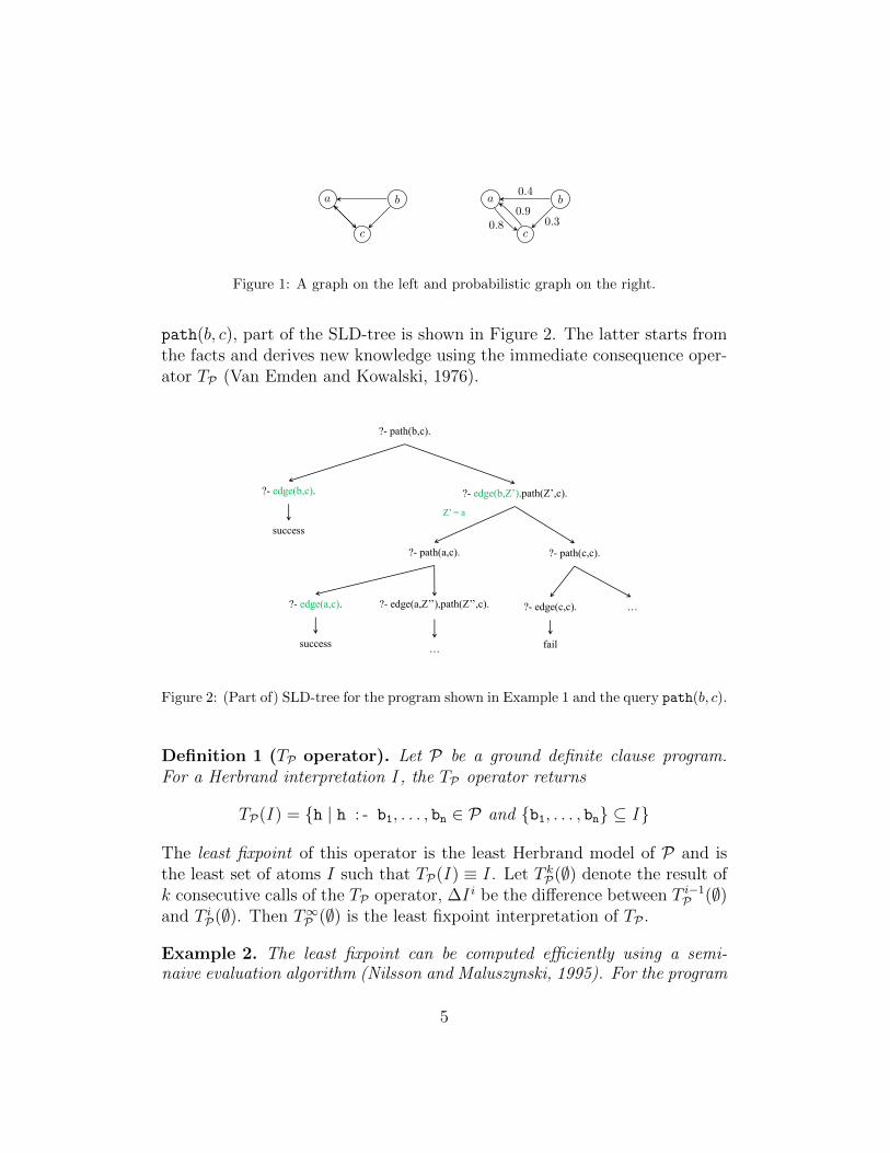
path(b, c), part of the SLD-tree is shown in Figure 2. The latter starts fromthe facts and derives new knowledge using the immediate consequence oper-ator TP (Van Emden and Kowalski, 1976).
?- path(b,c).
?- edge(b,c). ?- edge(b,Z’),path(Z’,c).
?- path(a,c). ?- path(c,c).
?- edge(a,c).
success
?- edge(c,c).
fail
?- edge(a,Z’’),path(Z’’,c). …
success Z’ = a
…
Figure 2: (Part of) SLD-tree for the program shown in Example 1 and the query path(b, c).
Definition 1 (TP operator). Let P be a ground definite clause program.For a Herbrand interpretation I , the TP operator returns
TP(I ) = {h | h : - b1, . . . , bn ∈ P and {b1, . . . , bn} ⊆ I }
The least fixpoint of this operator is the least Herbrand model of P and isthe least set of atoms I such that TP(I ) ≡ I . Let T kP(∅) denote the result ofk consecutive calls of the TP operator, ∆I i be the difference between T i−1
P (∅)and T iP(∅). Then T∞P (∅) is the least fixpoint interpretation of TP .
Example 2. The least fixpoint can be computed efficiently using a semi-naive evaluation algorithm (Nilsson and Maluszynski, 1995). For the program
5
given in Example 1, this results in:
I 0 = ∅∆I 1 = {e(b, a), e(b, c), e(a, c), e(c, a)}∆I 2 = {p(b, a), p(b, c), p(a, c), p(c, a)}∆I 3 = {p(a, a), p(c, c)}∆I 4 = ∅
and T∞P (∅) =⋃i ∆I i is the least Herbrand model as given above.
Property 1. Employing the TP operator on a subset of the least fixpointleads again to the same least fixpoint:
∀I ⊆ T∞P (∅) : T∞P (I ) = T∞P (∅)
Property 2. Adding a set of definite clauses P ′ to program P leads to asuperset of the least fixpoint for P:
T∞P (∅) ⊆ T∞P∪P ′(∅)
2.2. Beyond Definite Clause Programs
A normal logic program extends a definite clause program and allows fornegation, i.e., it is a finite set of normal clauses of the form h :− b1, ..., bnwhere h are atoms and the bi are literals. A literal is an atom (positiveliteral) or its negation (negative literal). The TP operator for definite clauseprograms can be generalized towards stratified normal logic programs, wherethe rules in the program are partitioned according to their strata (Nilssonand Maluszynski, 1995). Let Ph be the subset of clauses in P where h is thehead, then a stratified program is defined as follows:
Definition 2 (Stratified Program). A normal logic program P is said tobe stratified if there exists a partitioning P1 ∪ · · · ∪ Pm of P such that:
if h : - . . . , b, . . . ∈ Pi then Pb ⊆ P1 ∪ · · · ∪ Piif h : - . . . ,¬b, . . . ∈ Pi then Pb ⊆ P1 ∪ · · · ∪ Pi−1
The TP operator for normal logic programs is defined as:
TP(I ) = {h | h : - b1, . . . , bn ∈ P and I |= b1, . . . , bn}
6

where I |= bi if bi ∈ I and I |= ¬bi if bi /∈ I . Then, the canonical model1
can be obtained by iteratively computing the fixpoint for each stratum. LetIi be the Herbrand interpretation for stratum i, the canonical model for astratified program with m strata is computed as:
I1 = T∞P1(∅)
I2 = T∞P2(I1) ∪ I1
...
Im = T∞Pm(Im−1) ∪ Im−1
and T∞P (∅) = Im .
Example 3. Consider the following normal logic program with two strata:
P1
sprinklerOn.rain : - cloudy.wetGrass : - rain.
P2
{sprinkler : - ¬cloudy, sprinklerOn.wetGrass : - sprinkler.
for which computing the canconical model results in:
I1 = {sprinklerOn}I2 = {sprinkler, wetGrass} ∪ I1
and T∞P (∅) = {sprinklerOn, sprinkler, wetGrass}.
2.3. Probabilistic Logic Inference
Most probabilistic logic programming languages (e.g., ProbLog, PRISM,ICL) are based on Sato’s distribution semantics (Sato, 1995). In this paper,we use ProbLog as it is the simplest of these languages.
A ProbLog program P consists of a set R of rules and a set F of proba-bilistic facts. Without sacrificing generality, we assume that no probabilisticfact unifies with a rule head. A ProbLog program specifies a probability dis-tribution over its Herbrand interpretations, also called possible worlds. Every
1For a full discussion of the semantics of general logic programs, we refer to Van Gelderet al. (1991).
7
grounding fθ of a probabilistic fact p : : f independently takes the value true(with probability p) or false (with probability 1− p). For ease of notation,we assume that F is ground.
Example 4. Our program given in Example 1 can be extended with proba-bilities (see also Figure 1) in the following way:
0.4 : : edge(b, a). 0.3 : : edge(b, c).
0.8 : : edge(a, c). 0.9 : : edge(c, a).
path(X, Y ) : - edge(X, Y ).
path(X, Y ) : - edge(X,Z), path(Z, Y ).
The probabilistic facts represent that edges between two nodes are only truewith a certain probability. As a consequence, the rules now express a proba-bilistic path.
A total choice C ⊆ F assigns a truth value to every ground probabilis-tic fact, and the corresponding logic program C ∪ R has a canonical model(Fierens et al., 2015); the probability of this model is that of C. Interpreta-tions that do not correspond to any total choice have probability zero. Theprobability of a query q is then the sum over all total choices whose programentails q:
Pr(q) :=∑
C⊆F :C∪R|=q
∏fi∈C
pi ·∏
fi∈F\C
(1− pi) . (1)
As enumerating all total choices entailing the query is infeasible, state-of-the-art ProbLog inference reduces the problem to that of weighted modelcounting (Fierens et al., 2015). For a formula λ over propositional variablesV and a weight function w(·) assigning a real number to every literal for anatom in V , the weighted model count is defined as
WMC(λ) :=∑
I⊆V :I|=λ
∏a∈I
w(a) ·∏a∈V \I
w(¬a) . (2)
The reduction assigns w(fi) = pi and w(¬fi) = 1− pi for probabilistic factspi : : fi, and w(a) = w(¬a) = 1 else. For a query q, it constructs a formula λsuch that for every total choice C ⊆ F , C ∪ {λ} |= q ⇔ C ∪R |= q. While λmay use variables besides the probabilistic facts, e.g., variables correspondingto the atoms in the program, their values have to be uniquely defined for eachtotal choice.
8
Example 5. Consider the sprinkler program introduced in Example 3 butnow, sprinklerOn and cloudy are probabilistic facts:
0.7 : : sprinklerOn. 0.2 : : cloudy.
converting the program results in the following propositional formula:
rain↔ cloudy.
∧ sprinkler↔ ¬cloudy ∧ sprinklerOn.∧ wetGrass↔ rain ∨ sprinkler.
with w(sprinklerOn) = 0.7, w(¬sprinklerOn) = 0.3, w(cloudy) = 0.2 andw(¬cloudy) = 0.8.
We briefly discuss the key steps of the sequential WMC-based approach,and refer to Fierens et al. (2015) for full details. First, the relevant groundprogram, i.e., all and only those ground clauses that contribute to somederivation of a query (and evidence), is obtained using backward reason-ing. Next, the ground program is converted to a propositional formula inConjunctive Normal Form (CNF), which is finally passed to an off-the-shelfsolver for weighted model counting.
Example 6. For the logic program given in Example 1 and a query p(a, c),we would obtain the following ground program:
path(a, c) : - edge(a, c).
path(a, c) : - edge(a, c), path(c, c).
path(c, c) : - edge(c, a), path(a, c).
For acyclic rules, the conversion step is straightforward and only requiresto take Clark’s completion (Clark, 1978). For programs with cyclic rules,however, the conversion step is more complicated and requires additionalvariables and clauses to correctly capture the semantics of every cycle. Thiscan be done by rewriting the ground program.
Example 7. We can correctly break the cycles by rewriting the ground pro-gram from Example 6 in the following way:
path(a, c) : - edge(a, c).
path(a, c) : - edge(a, c), path(c, c).
path(c, c) : - edge(c, a), aux path(a, c).
aux path(a, c) : - edge(a, c).
9

The resources needed for the conversion step, as well as the size of theresulting CNF, greatly increase with the number of cycles in the groundprogram. For example, for a fully connected graph with only 10 nodes theconversion algorithm implemented in ProbLog returns a CNF with 26995variables and 109899 clauses.
Once the ground program is completely converted into a CNF formula, itcan be fed to any state-of-the art weighted model counter that supports thisstandard input format. One of the popular approaches for weighted modelcounting is supported by knowledge compilation.
2.4. Knowledge Compilation
For probabilistic inference it is common to compile the obtained propo-sitional formula into a target language for which WMC is polynomial in thesize of the representation (Darwiche and Marquis, 2002; Chavira and Dar-wiche, 2008). The most general language that efficiently supports WMC isdeterministic decomposable negation normal form (d-DNNF). The proper-ties of d-DNNF state that disjunctions are required to be deterministic, i.e.children of disjunctions cannot be true at the same time, and conjunctionsneed to be decomposable, i.e. children of conjunctions are not allowed toshare variables. Most of the d-DNNF compilers, such as c2d or DSHARP,require a CNF formula as input.
Sentential decision diagram (SDD) (Darwiche, 2011) is a recently intro-duced target representation that is a strict subset of d-DNNF. An SDD isof the form (p1 ∧ s1) ∨ · · · ∨ (pn ∧ sn) where each pair (pi ∧ si) is called anelement, the pi are called primes and the si are subs. Primes and subs arethemselves SDDs and the primes are consistent, mutually exclusive and ex-haustive. These properties are stronger than the ones for d-DNNF, allowingSDDs to efficiently support Boolean operations on formulas by means of anapply operator. More concretely, two SDDs (p1 ∧ s1) ∨ · · · ∨ (pn ∧ sn) and(p′1 ∧ s′1)∨ . . . (p′n ∧ s′n) can be combined with a boolean operator ◦ ∈ {∨,∧}as follows (p1 ∧ p′1 ∧ s1 ◦ s′1) ∨ · · · ∨ (pn ∧ p′n ∧ sn ◦ s′n), only requiring lin-ear time and space. Moreover, compressed SDDs are canonical leading to apractical efficient incremental compilation when performing a large numberof recursive apply operations (Van den Broeck and Darwiche, 2015; Choi etal., 2013). Hence, SDDs allow to be efficiently compiled in an incremental(bottom-up) way and do not strictly require to first construct a formula inCNF.
10

To conclude, we note that ordered binary decision diagram (OBDD) is asubset of SDD and also efficiently supports an apply operator. The advantageof SDD is that it comes with size upper bounds based on treewidth whichare tighter than the size upper bounds based on pathwidth for OBDDs.
3. The TcP Operator
We now develop the formal basis of our approach. For ease of notation, wefirst only consider definite clause programs and treat normal logic programstowards the end of this section.
3.1. Definite Clause Programs
The incentive of our inference algorithm is to interleave formula construc-tion and compilation by means of forward reasoning. The two advantages arethat (a) the conversion to propositional logic happens during rather than af-ter reasoning within the logic programming semantics, avoiding the expensiveintroduction of additional variables and propositions, and (b) at any time inthe process, the current formulas provide hard bounds on the probabilities.
Although forward reasoning naturally considers all consequences of a pro-gram, using the relevant ground program allows us to restrict the approachto the queries of interest. As common in probabilistic logic programming,we assume the finite support condition, i.e., the queries depend on a finitenumber of ground probabilistic facts.
We use forward reasoning to build a formula λa for every atom a ∈ A suchthat λa exactly describes the total choices C ⊆ F for which C∪R |= a. Suchλa can be used to compute the probability of a via WMC (cf. Section 2.3).
Definition 3 (Parameterized interpretation). A parameterized interpre-tation I of a ground probabilistic logic program P with probabilistic facts Fand atoms A is a set of tuples (a, λa) with a ∈ A and λa a propositionalformula over F expressing in which interpretations a is true.
Example 8. For the program shown in Example 4, the parameterized inter-pretation is:
{(e(b, a), λe(b,a)
),(e(b, c), λe(b,c)
), (e(a, c), λe(a,c)
), (e(c, a), λe(c,a)
),
(p(b, a), λp(b,a)
),(p(b, c), λp(b,c)
), (p(a, c), λp(a,c)
), (p(c, a), λp(c,a)
),
(p(a, a), λp(a,a)
),(p(c, c), λp(c,c)
)}.
11
and, for instance, λe(b,a) = e(b, a) since e(b, a) is true in exactly those worldswhere the total choice includes this edge, and λp(b,c) = e(b, c)∨[e(b, a)∧e(a, c)]since p(b, c) is true in exactly those worlds where the total choice includesthe direct edge or the two-edge path over a.
A naive approach to construct the λa would be to compute Ii = T∞R∪Ci(∅)
for every total choice Ci ⊆ F and to set λa =∨i:a∈Ii
∧f∈Ci
f , that is, thedisjunction explicitly listing all total choices contributing to the probabilityof a. Clearly, this requires a number of fixpoint computations exponentialin |F|, and furthermore, doing these computations independently does notexploit the potentially large structural overlap between them.
Therefore, we introduce the TcP operator. It generalizes the TP operatorto work on the parameterized interpretation and builds, for all atoms in par-allel on demand, formulas that are logically equivalent to the λa introducedabove. For ease of notation, we assume that every parameterized interpre-tation implicitly contains a tuple (true,>), and, just as in regular interpre-tations, we do not list atoms with λa ≡ ⊥. Thus, the empty set implicitlyrepresents the parameterized interpretation {(true,>)}∪{(a,⊥)|a ∈ A} fora set of atoms A.
Definition 4 (TcP operator). Let P be a ground probabilistic logic pro-gram with probabilistic facts F and atoms A. Let I be a parameterized inter-pretation with pairs (a, λa). Then, the TcP operator is TcP(I) = {(a, λ′a) |a ∈ A} where
λ′a =
{a if a ∈ F∨
(a :- b1,...,bn)∈P(λb1 ∧ · · · ∧ λbn) if a ∈ A \ F .
Intuitively, where the TP operator (repeatedly) adds an atom a to the inter-pretation whenever the body of a rule defining a is true, the TcP operatoradds to the formula for a the description of the total choices for which the rulebody is true. In contrast to the TP operator, where a syntactic check sufficesto detect that the fixpoint is reached, the TcP operator requires a semanticfixpoint check for each formula λa, which we write as I i ≡ TcP(I i−1).
Definition 5 (Fixpoint of TcP). A parameterized interpretation I is a fix-point of the TcP operator if and only if for all a ∈ A, λa ≡ λ′a, where λa andλ′a are the formulas for a in I and TcP(I), respectively.
12

It is easy to verify that for F = ∅, i.e., a ground logic program P , the iter-ative execution of the TcP operator directly mirrors that of the TP operator,representing atoms as (a,>). We use λia to denote the formula associatedwith atom a after i iterations of TcP starting from ∅. We use SDDs toefficiently represent the formulas λa as will be discussed in Section 4.
Example 9. Applying TcP to the program given in Example 4 results in thefollowing sequence:
The first application of TcP sets:
λ1e(b,a) = e(b, a), λ1
e(a,c) = e(a, c), λ1e(b,c) = e(b, c), λ1
e(c,a) = e(c, a)
These remain the same in all subsequent iterations.The second application of TcP starts adding formulas for path atoms,
which we illustrate for just two atoms:
λ2p(b,c) = λ1
e(b,c) ∨ (λ1e(b,a) ∧ λ1
p(a,c)) ∨ (λ1e(b,c) ∧ λ1
p(c,c))
= e(b, c) ∨ (e(b, a) ∧ ⊥) ∨ (e(a, c) ∧ ⊥) ≡ e(b, c)
λ2p(c,c) = (λ1
e(c,a) ∧ λ1p(a,c)) = (e(c, a) ∧ ⊥) ≡ ⊥
That is, the second step considers paths of length at most 1 and adds (p(b, c), e(b, c))to the parameterized interpretation, but does not add a formula for p(c, c), asno total choices making this atom true have been found yet.
The third iteration, adds information on paths of length at most 2:
λ3p(b,c) = λ2
e(b,c) ∨ (λ2e(b,a) ∧ λ2
p(a,c)) ∨ (λ2e(b,c) ∧ λ2
p(c,c))
≡ e(b, c) ∨ (e(b, a) ∧ e(a, c))λ3p(c,c) = (λ2
e(c,a) ∧ λ2p(a,c)) ≡ (e(c, a) ∧ e(a, c))
Intuitively, TcP keeps adding longer sequences of edges connecting the cor-responding nodes to the path formulas, reaching a fixpoint once all acyclicsequences have been added.
Correctness. We show that for increasing i, TciP(∅) reaches a least fix-point Tc∞P (∅) where the λa are exactly the formulas needed to compute theprobability for each atom by WMC.
Theorem 1. For a ground probabilistic definite clause program P with prob-abilistic facts F , rules R and atoms A, let λia be the formula associated with
13

atom a in TciP(∅). For every atom a, total choice C ⊆ F and iteration i, wehave:
C |= λia → C ∪R |= a
Proof by induction: i = 1: easily verified. i→ i+1: easily verified for a ∈ F ;for a ∈ A \ F , let C |= λi+1
a , that is, C |=∨
(a :- b1,...,bn)∈P(λib1 ∧ · · · ∧ λibn
).
Thus, there is a a : - b1, . . . , bn ∈ P with C |= λibj for all 1 ≤ j ≤ n. By
assumption, C ∪R |= bj for all such j and thus C ∪R |= a. �
Corollary 1. After each iteration i, we have WMC(λia) ≤ Pr(a).
Theorem 2. For a ground probabilistic definite clause program P with prob-abilistic facts F , rules R and atoms A, let λia be the formula associated withatom a in TciP(∅). For every atom a and total choice C ⊆ F , there is an i0such that for every iteration i ≥ i0, we have
C ∪R |= a ↔ C |= λia
Proof: ←: Theorem 1. →: C ∪ R |= a implies ∃i0∀i ≥ i0 : a ∈ T iC∪R(∅).We further show ∀j : a ∈ T jC∪R(∅) → C |= λja by induction. j = 1: easilyverified. j → j + 1: easily verified for a ∈ F ; for other atoms, a ∈ T j+1
C∪R(∅)implies there is a rule a : - b1, . . . , bn ∈ R such that ∀k : bk ∈ T jC∪R(∅). Byassumption, ∀k : C |= λjbk , and by definition, C |= λj+1
a . �Thus, for every atom a, the λia reach a fixpoint λ∞a exactly describing the
possible worlds entailing a, and the TcP operator therefore reaches a fixpointwhere for all atoms Pr(a) = WMC(λ∞a ).2
Conditional Probabilities. Once a fixpoint is reached, conditional prob-abilities can be computed using Bayes’ rule. The probability of a query q,given a set E of observed atoms (evidence atoms) and a vector e of observedtruth values, is computed as:
Pr(q|E = e) =WMC(λ∞q ∧ λ∞e )
WMC(λ∞e )with λ∞e =
∧e∈e
λ∞e
Hence, computing conditional probabilities additionally requires the con-struction of a formula λ∞e that represents the evidence e.
2The finite support condition ensures this happens in finite time.
14
3.2. Normal Logic Programs
The correspondence with the TP operator allows us to extend the TcPoperator towards stratified normal logic programs (Sec. 2.2). To do so, weapply the TcP operator stratum by stratum, that is, we first have to reach afixpoint for Pi before considering the rules in Pi+1. Let Ii be the parametrizedinterpretation for stratum i, the set of formulas for a stratified program withm strata is obtained by:
I1 = Tc∞P1(∅)
I2 = Tc∞P2(I1)
...
Im = Tc∞Pm(Im−1)
Following the definition of stratified programs, the formula for a negativeliteral ¬a is only required once a fixpoint for the positive literal a has beenreached. Hence, λ¬a can be obtained as ¬λa.
4. Anytime Inference
Probabilistic inference iteratively calls the TcP operator until the fixpointis reached. This involves incremental formula construction (cf. Definition 4)and equivalence checking (cf. Definition 5).
An efficient realization of our evaluation algorithm is obtained by repre-senting the formulas in the interpretation I by means of a Sentential DecisionDiagram (SDD), which can handle the required operations efficiently (Dar-wiche, 2011). Hence, we can replace each λa in Definition 4 by its equivalentSDD representation Λa and each of the Boolean operations by the Apply-operator for SDDs which, given ◦ ∈ {∨,∧} and two SDDs Λa and Λb, returnsan SDD equivalent with (Λa ◦ Λb).
4.1. TP-Compilation
The TcP operator is, by definition, called on I. To allow for differentevaluation strategies, however, we propose a more fine-grained algorithmwhere, in each iteration, the operator is only called on one specific atoma, i.e., only the rules for which a is the head are evaluated, denoted byTcP(a, I i−1). Note that, in case of normal logic programs, we only considerthe rules within one stratum. Each iteration i of TP-compilation consists oftwo steps;
15
1. Select an atom a ∈ A.
2. Compute I i = TcP(a, I i−1)
The result of Step 2 is that only the formula for atom a is updated and, foreach of the other atoms, the formula in I i is the same as in I i−1. It is easy toverify that TP-compilation reaches the fixpoint Tc∞P (∅) in case the selectionprocedure frequently returns each of the atoms in P .
4.2. Lower Bound
Following Theorem 1, we know that, after each iteration i, WMC(λia)is a lower bound on the probability of atom a, i.e., WMC(λia) ≤ Pr(a) =WMC(λ∞a ), which holds for definite clause programs as well as for stratifiednormal logic programs. To quickly increase WMC(λia) and, at the same time,avoid a blow-up of the formulas in I, the selection procedure we employ picksthe atom which maximizes the following heuristic value:
WMC(Λia)−WMC(Λi−1
a )
φa · (Size(Λia)− Size(Λi−1
a ))/Size(Λi−1a )
where Size(Λ) denotes the number of edges in SDD Λ and φa adjusts for theimportance of a in proving queries.
Concretely, Step 1 of TP-compilation calls TcP(a, I i−1) for each a ∈ A,computes the heuristic value and returns the atom a′ for which this valueis the highest. Then, Step 2 performs I i = TcP(a′, I i−1). Although thereis overhead involved in computing the heuristic value, as many formulas arecompiled without storing them, this strategy works well in practice.
We take as value for φa the minimal depth of the atom a in the SLD-treefor each of the queries of interest. This value is a measure for the influence ofthe atom on the probability of the queries. For our example, and the queryp(b, c), the use of φa would give priority to compile p(b, c) as it is on top ofthe SLD-tree (see Figure 2). Without φa, the heuristic would give priorityto compile p(a, c) as it has the highest probability.
4.3. Upper bound
To compute an upper bound for definite clause programs, we select F ′ ⊂F and treat each f ∈ F ′ as a logical fact rather than a probabilistic fact, thatis, we conjoin each λa with
∧f∈F ′ λf . In doing so, we simplify the compilation
step of our algorithm, because the number of possible total choices decreases.Furthermore, at a fixpoint, we have an upper bound on the probability of the
16
atoms, i.e., WMC(λ∞a |λF ′) ≥ Pr(a), because we overestimate the probabilityof each fact in F ′.
Randomly selecting F ′ ⊂ F does not yield informative upper bounds(they are close to 1). As a heuristic, we compute for each of the facts theminimal depth in the SLD-trees of the queries of interest and select for F ′all facts whose depth is smaller than some constant d. Hence, we avoid thequery to be deterministically true as for each of the proofs, i.e., traces inthe SLD-tree, we consider at least one probabilistic fact. This yields tighterupper bounds. For our example, and the query p(b, c), both of the edgesstarting in node b are at a depth of 1 in the SLD-tree (see Figure 2). Hence,it suffices to compile only them, and treat both other edges as logical facts,to obtain an upper bound smaller than 1.
Discussion. Computation of the lower bounds is also valid for programswith negation but rules need to be compiled according to their stratification.Computation of our upper bounds only holds for definite clause programs,i.e., programs without negation, and is similar in spirit to the upper boundsof Poole (1993) and De Raedt et al. (2007). As computation of the lower andupper bound operates on different formulas, an anytime algorithm shouldalternate between compiling these formulas.
5. Extensions of Tp-Compilation
Modeling real-world applications might require the inclusion of time inan implicit way, e.g. with program updates, or explicit way, e.g. dynamicmodels. We now show how TP-compilation allows us to deal efficiently withthese models.
5.1. Inference with Program Updates
A probabilistic logic program typically represents a stationary model,that is, the set of rules R as well as the set of facts F is fixed. For manyapplications, however, the program only expresses all available information atone specific moment in time while the underlying process constantly evolves.As an example one can think of a probabilistic graph, as shown in Figure 1,where new edges and nodes are discovered over time, while others disappear.
To cope with new information, the set of facts F is updated while theset of (non-ground) rules R remains unchanged. Adding facts leads to newclauses in the ground program and removing facts removes clauses from the
17

grounded program. One way to deal with program changes is to recompilethe complete program from scratch after each update of F . In case F changesonly marginally, however, a more efficient approach is to reuse past compila-tion results. This can be achieved using the TcP operator, which allows foradding clauses to and removing clauses from the program. We only considerprogram updates for definite clause programs as for normal logic programswe will have to restart compilation from the lowest strata affected by theupdate.
Adding Clauses. For definite clause programs, we know that employing theTP operator on a subset of the fixpoint reaches the fixpoint (see Property 1).Moreover, adding definite clauses leads to a superset of the fixpoint (seeProperty 2). Hence, it is safe to restart the TP operator from a previousfixpoint after adding clauses. Assume the set of facts F is extended toF ′, then we have T∞R∪F ′(∅) = T∞R∪F ′(T
∞R∪F(∅)). Due to the correspondence
established in Theorem 2, this also applies to TcP . For our example, wecould add 0.1 : : e(a, b) and the corresponding ground rules. This leads tonew paths, such as p(b, b), and increases the probability of existing paths,such as p(a, c).
Removing Clauses. When removing clauses from a definite clause pro-gram, atoms in the fixpoint may become invalid. We therefore reset the com-puted fixpoints for all total choices where the removed clause could have beenapplied. This is done by conjoining each of the formulas in the parametrizedinterpretation with the negation of the formula for the head of the removedclause. Let I denote the parametrized interpretation and H the set of atomsin the head of a removed clause, the new parameterized interpretation I ′ isobtained as:
I ′ = {(a, λ′a) | (a, λa) ∈ I with λ′a = λa ∧∧h∈H
¬λh}
Then, we restart the TcP operator from the adjusted parametrized interpre-tation I ′, to recompute the fixpoint for the total choices that were removed.For our example, if we remove 0.5 : : e(b, c) and the rules containing this edge,we are removing a possible path from b to c and thus decreasing the proba-bility of p(b, c).
18
5.2. Inference in Dynamic Models
Probabilistic logic programs allow us to represent stochastic processes bymeans of a dynamic model (Nitti et al., 2013; Thon et al., 2011). To do so, oneexplicitly inserts time such that each rule is of the form ht :− b1,t1, ..., bn,tn,where t, t1, . . . , tn denotes the time step to which the corresponding atombelongs. In this paper, we assume that the first-order Markov property holds,allowing us to rewrite the rules as ht :− b1,t, . . . , bm,t, bm+1,t−1, . . . bn,t−1, i.e.,each atom can only depend on atoms from the same or previous time step.Note that this also implies that cycles cannot range over different time steps.
Example 10. Consider the following probabilistic logic program3 represent-ing a dynamic social network:
0.2 : : coldOutsidet.
0.4 : : staySick(X)t.
sick(X)t : - coldOutsidet.
sick(X)t : - friends(X, Y ), sick(Y )t.
sick(X)t : - sick(X)t−1, staySick(X)t.
We assume the friends relation remains constant over time, and thereforedrop the time index for these atoms.
In practice, one distinguishes an initial model from the transition model.The former expresses the prior distribution, i.e., the distribution for the firsttime step, while the latter latter serves as a template for all subsequent time-steps. As the transition model is the one that repeats over time, we focus onthe latter.
Inference. One way to perform inference in a dynamic model is by meansof unrolling, i.e. one grounds the program for a set of queries and runs astandard inference algorithm. It is well-known, however, that this approachscales poorly when inference is required for a large number of time steps.A more efficient alternative is obtained by exploiting the repeated structurethat is inherently present in dynamic models (Murphy, 2002). We shortlyreview the key ideas of inference in dynamic models and refer to Murphy(2002) and Vlasselaer et al. (2016) for more details.
3The model can be represented as a PLP by including for each atom a time argument T.
19

The most common inference task in dynamic models is that of filtering.Here, the goal is to compute the probability of a query q at time step tgiven evidence (observations) up to time step τ , i.e., one aims to computePr(qt|e1:τ ) with τ ≤ t. This task can be performed efficiently by repeatedlycomputing the forward message for each time step t. The forward messageis the joint probability distribution over all atoms that d-separate the pastfrom the future, i.e., knowing the joint distribution over all these atomsmakes the future independent of the past. The set of atoms over which thejoint distribution has to be computed is referred to as the interface, which wedenote as It. The forward message can be computed recursively as follows:
Pr(It|e1:t) =∑
it−1∈It−1
Pr(It|it−1, et) Pr(it−1|e1:t−1) (3)
with et the truth values of the observed atoms at time t and it−1 onetruth-value assignment to atoms in It−1. Once we have Pr(It|e1:t), we cancompute Pr(qt+1|e1:t+1).
Example 11. For the dynamic model presented in Example 10 and a domainof three persons, ann, bob and cin, the interface is the following set of threeatoms:
It = {sick(ann)t, sick(bob)t, sick(cin)t}.
The forward message involves computing the probability of each possible valueassignment of the interface given the previous interface and evidence:
Pr(sick(ann)t ∧ sick(bob)t ∧ sick(cin)t | It−1, et
),
Pr(sick(ann)t ∧ sick(bob)t ∧ ¬sick(cin)t | It−1, et
),
. . .
Pr(¬sick(ann)t ∧ ¬sick(bob)t ∧ ¬sick(cin)t | It−1, et
)Dynamic TP-compilation. We now extend our TP-compilation approachto efficiently perform inference in dynamic domains. In doing so, we candistinguish the following two phases:
• Offline phase: Use TP-compilation to compile the transition model.The resulting parametrized interpretation I contains a tuple (a, λa) foreach atom a in the transition model. The formulas λa will then serveas a template for each time-step that inference is required. The offlinephase only has to be performed once.
20

• Online phase: Iterate over time-steps t and compute the forward mes-sage. This includes extending the template formulas Λa to adjust forthe situation, i.e. the evidence, at time t.
Computation of the forward message at time t requires extending thetemplate formulas Λa to take into account the evidence for time-step t, de-noted with et, as well as the distribution from t − 1. We use Λt
a to denotethe adjusted formula of atom a for time step t. Let it be one truth-valueassignment to atoms in It, its conditional probability is computed as:
Pr(it|e1:t) =WMC
(∧i∈it Λt
i
)WMC(Λt
et)(4)
withΛti =
∨ij∈I
((Λi ∧ Λet)|ij
)∧ state j
t−1 ∧ ij (5)
where Λet is the formula representing the evidence, as defined before, and Λ|idenotes that the formula Λ is conditioned on the values in i. Conditioningtransforms the formula by replacing all variables V in Λ with their assign-ment in v and propagates these values while preserving the properties ofthe formula (Darwiche and Marquis, 2002). The auxiliary variable statejt−1
is required to correctly include the distribution from t − 1 (cf. Equation3) and the weight function sets w(statejt−1) = Pr(ijt−1|e1:t−1). The forwardmessage (the complete distribution) is obtained by repeating Equation 4 foreach it ∈ It.
To push more of the computational effort towards the offline phase, wecould rewrite Equation 5 as:
Λti =
∨ij∈I
((Λi|ij
)∧(Λet |ij
)∧ state j
t−1 ∧ ij (6)
such that Λi|ij has to be computed only once.
Dealing with Evidence. The key difference of dynamic TP-compilationcompared to the structural interface algorithm (SIA) introduced by Vlasse-laer et al. (2016) is how evidence is treated. The incentive of SIA is to pushas much of the computational overhead, i.e., all compilation steps, into theoffline phase. This requires the compilation of one large formula that con-tains a variable for each of the atoms in the transition model, including the
21
ones that are (potentially) observed. Then, the forward message is computedby accordingly setting weights and requires an exponential number of WMCcalls.
With our TP-compilation approach, on the other hand, we do not includeevidence by setting weights but adjust the template formulas Λa to explicitlycontain the evidence. This requires, for each time step t, to conjoin thetemplate formulas with Λet , that is, the formula representing the evidence(see Equation 5). Although this approach requires an additional compilationstep within the online phase, which might be computationally expensive,representing the evidence explicitly allows us to exploit local structure, inthe form of determinism, in the forward message. Indeed, if w(statejt−1) = 0or if (Λi ∧ Λet) ≡ ⊥, Equation 5 simplifies significantly. Hence, we avoid anexponential representation of the forward message in case evidence introducesdeterminism in Pr(It|e1:t).
Pushing Λi|ij towards the offline phase, as done by Equation 6, still re-quires an exponential representation and does not maximally exploit poten-tial determinism in the forward message. Hence, Equation 6 is only beneficialin case there is not enough determinism to compensate for the computationaloverhead in Equation 5. We refer to Equation 5 as flexible and to Equation6 as fixed dynamic TP compilation.
Discussion. The above introduced approach only considers exact inferencefor dynamic domains and is, in worst-case, exponential in the number ofatoms in the interface. A topic of future work is to investigate how we canextend this approach towards bounded approximate inference as presentedby Boyen and Koller (1998).
6. Experimental Results
Our experiments address the following questions:
Q1 How does TP-compilation compare to exact sequential WMC approaches?
Q2 How does TP-compilation compare to anytime sequential approaches?
Q3 What is the impact of approximating the model?
Q4 Can we efficiently deal with program updates?
Q5 Can we efficiently exploit evidence in dynamic domains?
22

We compute relevant ground programs as well as CNFs (where applicable)following Fierens et al. (2015) and use the SDD package developed at UCLA4.Experiments are run on a 3.4 GHz machine with 16 GB of memory. Ourimplementation is available as part of the ProbLog package5.
6.1. Exact Inference
We use datasets of increasing size from two domains:Smokers. Following Fierens et al. (2015), we generate random power
law graphs for the standard ‘Smokers’ social network domain. Cycles in theprogram are introduced by the following rule:
smokes(X) : - friends(X, Y ), smokes(Y ).
Alzheimer. We use series of connected subgraphs of the Alzheimer networkof De Raedt et al. (2007), starting from a subsample connecting the twogenes of interest ‘HGNC 582’ and ‘HGNC 983’, and adding nodes that areconnected with at least two other nodes in the graph. The logic program(i.e., the set of rules) is similar to the one we used in our example (see Figure1) and cycles are introduced by the second rule for path.
The relevant ground program is computed for one specific query as wellas for multiple queries. For the Smokers domain, this is cancer(p) for aspecific person p versus for each person. For the Alzheimer domain, this isthe connection between the two genes of interest versus all genes.
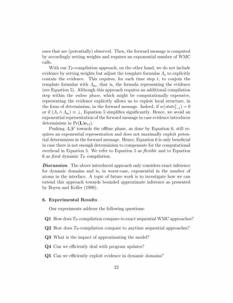
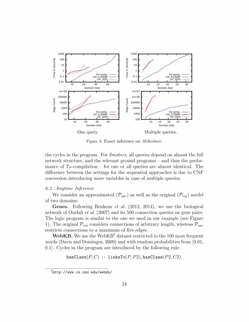
For the sequential approach, we perform WMC using either SDDs, or d-DNNFs compiled with c2d6 (Darwiche, 2004). For each domain size (#per-sons or #nodes) we consider nine instances with a timeout of one hour persetting. We report median running times and target representation sizes,using the standard measure of #edges for the d-DNNFs and 3 · #edges forthe SDDs. The results are depicted in Figure 3 and 4 and provide an answerfor Q1.
In all cases, the TP-compilation (Tp-comp) scales to larger domains thanthe sequential approach with both SDD (cnf SDD) and d-DNNF (cnf d-DNNF)and produces smaller compiled structures, which makes subsequent WMCcomputations more efficient. The smaller structures are mainly obtained be-cause our approach does not require auxiliary variables to correctly handle
4http://reasoning.cs.ucla.edu/sdd/5https://dtai.cs.kuleuven.be/problog/6http://reasoning.cs.ucla.edu/c2d/
23
0.01
0.1
1
10
100
1000
10 20 30 40
Tim
e in S
econds
Domain Size
Tp-comp.cnf_d-DNNF
cnf_SDD 0.01
0.1
1
10
100
1000
10 15 20 25 30
Tim
e in S
econds
Domain Size
Tp-comp.cnf_d-DNNF
cnf_SDD
10
100
1000
10000
100000
1e+06
10 20 30 40
Edge C
ount
Domain Size
Tp-comp.cnf_d-DNNF
cnf_SDD
One query.
100
1000
10000
100000
1e+06
1e+07
10 15 20 25 30
Edge C
ount
Domain Size
Tp-comp.cnf_d-DNNF
cnf_SDD
Multiple queries.
Figure 3: Exact inference on Alzheimer.
the cycles in the program. For Smokers, all queries depend on almost the fullnetwork structure, and the relevant ground programs – and thus the perfor-mance of TP-compilation – for one or all queries are almost identical. Thedifference between the settings for the sequential approaches is due to CNFconversion introducing more variables in case of multiple queries.
6.2. Anytime Inference
We consider an approximated (Papr) as well as the original (Porg) modelof two domains:
Genes. Following Renkens et al. (2012, 2014), we use the biologicalnetwork of Ourfali et al. (2007) and its 500 connection queries on gene pairs.The logic program is similar to the one we used in our example (see Figure1). The original Porg considers connections of arbitrary length, whereas Papr
restricts connections to a maximum of five edges.WebKB. We use the WebKB7 dataset restricted to the 100 most frequent
words (Davis and Domingos, 2009) and with random probabilities from[0.01,
0.1]. Cycles in the program are introduced by the following rule:
hasClass(P,C) : - linksTo(P, P2), hasClass(P2, C2).
7http://www.cs.cmu.edu/webkb/
24
0.01
0.1
1
10
100
1000
5 10 15 20 25
Tim
e in S
econds
Domain Size
Tp-comp.cnf_d-DNNF
cnf_SDD
0.01
0.1
1
10
100
1000
5 10 15 20 25
Tim
e in S
econds
Domain Size
Tp-comp.cnf_d-DNNF
cnf_SDD
10
100
1000
10000
100000
1e+06
1e+07
5 10 15 20 25
Edge C
ount
Domain Size
Tp-comp.cnf_d-DNNF
cnf_SDD
One query.
10
100
1000
10000
100000
1e+06
5 10 15 20 25
Edge C
ount
Domain Size
Tp-comp.cnf_d-DNNF
cnf_SDD
Multiple queries.
Figure 4: Exact inference on Smokers.
0.01
0.1
1
10
100
1000
10000
10 15 20 25 30
Tim
e in S
econds
Domain Size
Tp-comp.Tcp-inc.
Tcp-inc.-total
0.01
0.1
1
10
100
20 50 80 110 140
Tim
e in S
econds
Domain Size
Tp-comp.Tcp-inc.
Tcp-inc.-total
Figure 5: Program updates for Alzheimer (left) and Smokers (right).
Following Renkens et al. (2014), Papr is a random subsample of 150 pages.Porg uses all pages from the Cornell database. This results in a dataset with63 queries for the class of a page.
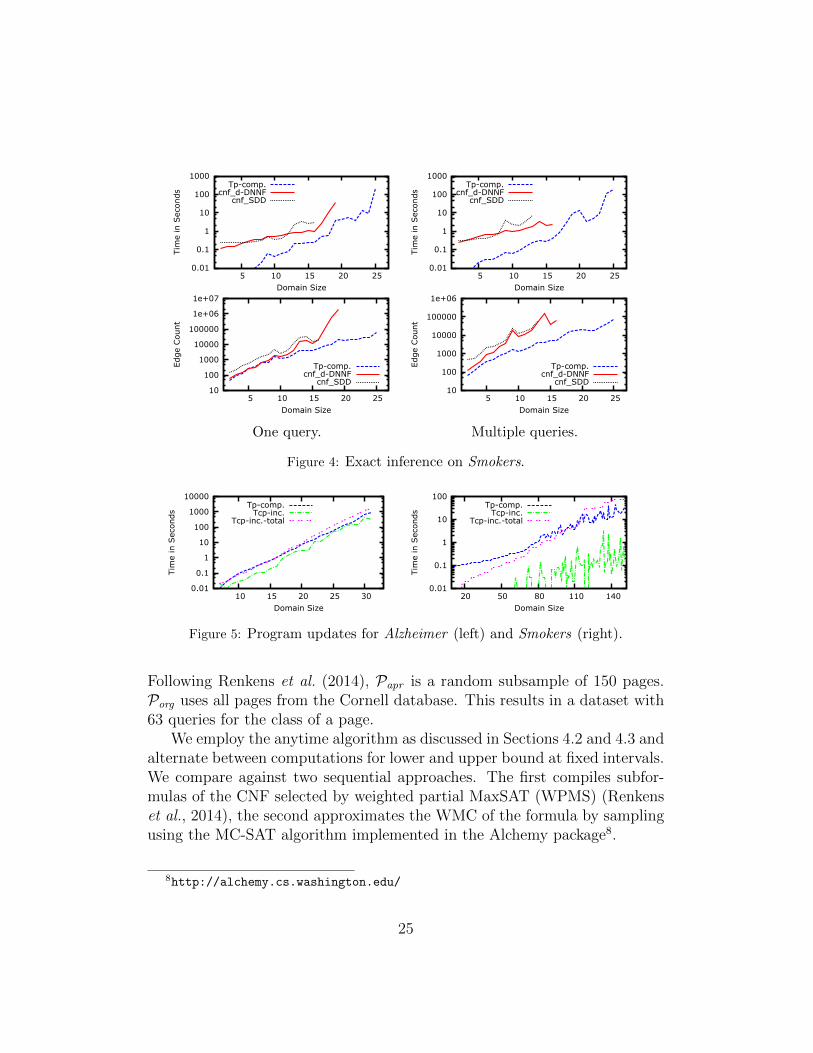
We employ the anytime algorithm as discussed in Sections 4.2 and 4.3 andalternate between computations for lower and upper bound at fixed intervals.We compare against two sequential approaches. The first compiles subfor-mulas of the CNF selected by weighted partial MaxSAT (WPMS) (Renkenset al., 2014), the second approximates the WMC of the formula by samplingusing the MC-SAT algorithm implemented in the Alchemy package8.
8http://alchemy.cs.washington.edu/
25
Papr Porg
WPMS TP -comp WPMS TP -comp
Gen
es
Almost Exact 308 419 0 30Tight Bound 135 81 0 207Loose Bound 54 0 0 263
No Answer 3 0 500 0
Web
KB Almost Exact 1 7 0 0
Tight Bound 2 34 0 19Loose Bound 2 22 0 44
No Answer 58 0 63 0
Table 1: Anytime inference: Number of queries with difference between bounds <0.01 (Almost Exact), in [0.01, 0.25) (Tight Bound), in [0.25, 1.0) (Loose Bound),and 1.0 (No Answer).
Papr Porg
MCsat5000 MCsat10000 MCsat
Gen
es In Bounds 150 151 0Out Bounds 350 349 0
N/A 0 0 500
Table 2: Anytime inference with MC-SAT: numbers of results within and outsidethe bounds obtained by TP -compilation on Papr , using 5000 or 10000 samples perCNF variable.
0
100
200
300
400
500
0 50 100 150 200 250 300
Num
ber
of Q
ueries
Time in Seconds
WPMS-0.001-errorWPMS-0.01-errorWPMS-0.05-error
Tp-comp.-0.001-errorTp-comp.-0.01-errorTp-comp.-0.05-error
Figure 6: Anytime inference on Genes with Papr : number of queries with bounddifference below threshold at any time.
Following Renkens et al. (2014), we run inference for each query sepa-rately. The time budget is 5 minutes for Papr and 15 minutes for Porg (ex-cluding the time to construct the relevant ground program). For MC-SAT,we sample either 5,000 or 10,000 times per variable in the CNF, which yieldsapproximately the same runtime as our approach. Results are depicted inTables 1, 2 and Figure 6 and allow us to answer Q2 and Q3.
26

Table 1 shows that TP-compilation returns bounds for all queries in allsettings, whereas WPMS did not produce any answer for Porg . The latteris due to reaching the time limit before conversion to CNF was completed.For the approximate model Papr on the Genes domain, both approachessolve a majority of queries (almost) exactly. Figure 6 plots the numberof queries that reached a bound difference below different thresholds againstthe running time, showing that TP-compilation converges faster than WPMS.Finally, for the Genes domain, Table 2 shows the number of queries wherethe result of MC-SAT (using different numbers of samples per variable in theCNF) lies within or outside the bounds computed by TP-compilation. Forthe original model, no complete CNF is available within the time budget; forthe approximate model, more than two thirds of the results are outside theguaranteed bounds obtained by our approach.
We further observed that for 53 queries on the Genes domain, the lowerbound returned by our approach using the original model is higher thanthe upper bound returned by WPMS with the approximated model. Thisillustrates that computing upper bounds on an approximate model does notprovide any guarantees with respect to the full model. On the other hand,for 423 queries in the Genes domain, TP-compilation obtained higher lowerbounds with Papr than with Porg , and lower bounds are guaranteed in bothcases.
In summary, we conclude that approximating the model can result inmisleading upper bounds, but reaches better lower bounds (Q3), and thatTP-compilation outperforms the sequential approaches for time, space andquality of result in all experiments (Q2).
6.3. Program Updates
We perform experiments on the Alzheimer domain discussed above, anda variant on the smokers domain. The smokers network has 150 persons andis the union of ten different random power law graphs with 15 nodes each.We consider the multiple queries setting only, and again report results fornine runs.
We compare our standard TP-compilation algorithm, which compiles thenetworks for each of the domain sizes from scratch, with the online algorithmdiscussed in Section 5.1. The results are depicted in Figure 5 and provide ananswer to Q4.
For the Alzheimer domain, which is highly connected, incrementally addingthe nodes (Tcp-inc) has no real benefit compared to recompiling the net-
27
work from scratch (Tp-comp) and, consequently, the cumulative time of theincremental approach (Tcp-inc-total) is higher. For the smokers domain,on the other hand, the incremental approach is more efficient compared torecompiling the network, as it only updates the subnetwork to which themost recent person has been added.
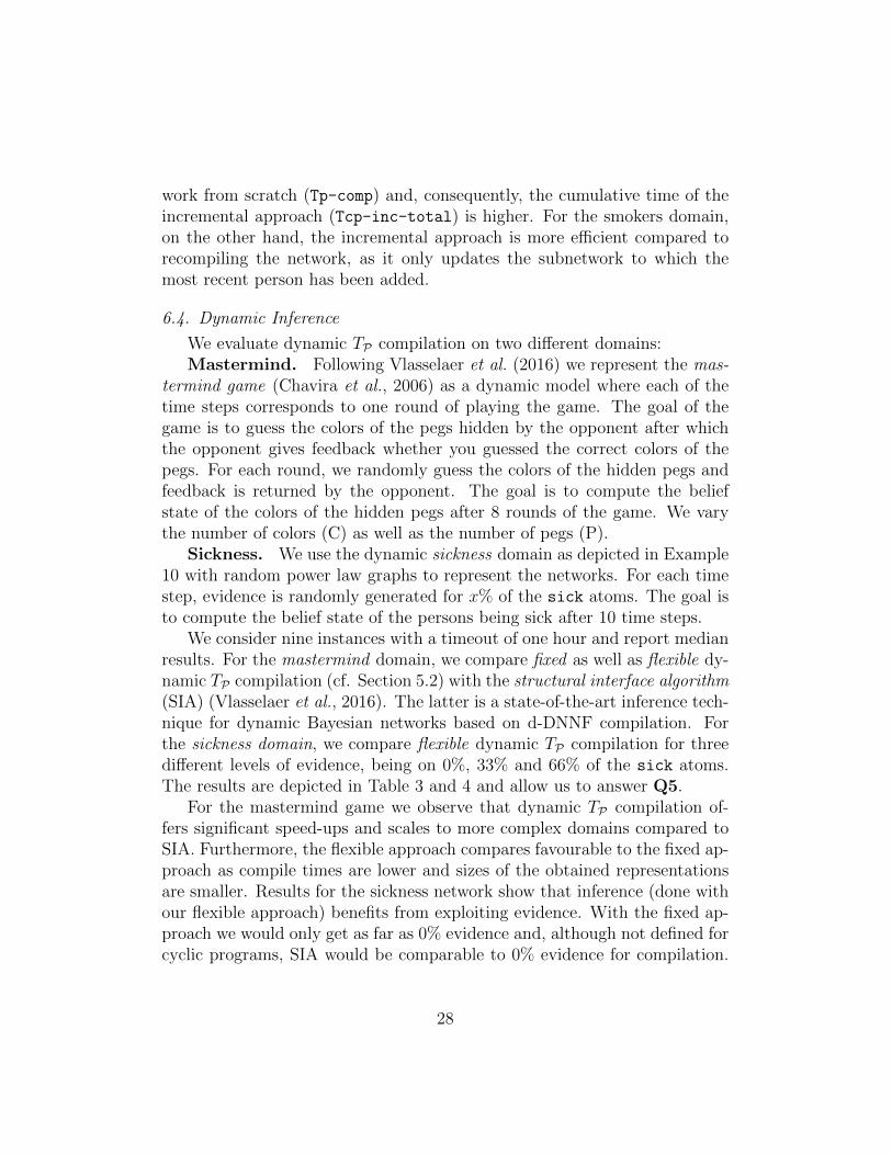
6.4. Dynamic Inference
We evaluate dynamic TP compilation on two different domains:Mastermind. Following Vlasselaer et al. (2016) we represent the mas-
termind game (Chavira et al., 2006) as a dynamic model where each of thetime steps corresponds to one round of playing the game. The goal of thegame is to guess the colors of the pegs hidden by the opponent after whichthe opponent gives feedback whether you guessed the correct colors of thepegs. For each round, we randomly guess the colors of the hidden pegs andfeedback is returned by the opponent. The goal is to compute the beliefstate of the colors of the hidden pegs after 8 rounds of the game. We varythe number of colors (C) as well as the number of pegs (P).
Sickness. We use the dynamic sickness domain as depicted in Example10 with random power law graphs to represent the networks. For each timestep, evidence is randomly generated for x% of the sick atoms. The goal isto compute the belief state of the persons being sick after 10 time steps.
We consider nine instances with a timeout of one hour and report medianresults. For the mastermind domain, we compare fixed as well as flexible dy-namic TP compilation (cf. Section 5.2) with the structural interface algorithm(SIA) (Vlasselaer et al., 2016). The latter is a state-of-the-art inference tech-nique for dynamic Bayesian networks based on d-DNNF compilation. Forthe sickness domain, we compare flexible dynamic TP compilation for threedifferent levels of evidence, being on 0%, 33% and 66% of the sick atoms.The results are depicted in Table 3 and 4 and allow us to answer Q5.
For the mastermind game we observe that dynamic TP compilation of-fers significant speed-ups and scales to more complex domains compared toSIA. Furthermore, the flexible approach compares favourable to the fixed ap-proach as compile times are lower and sizes of the obtained representationsare smaller. Results for the sickness network show that inference (done withour flexible approach) benefits from exploiting evidence. With the fixed ap-proach we would only get as far as 0% evidence and, although not defined forcyclic programs, SIA would be comparable to 0% evidence for compilation.
28
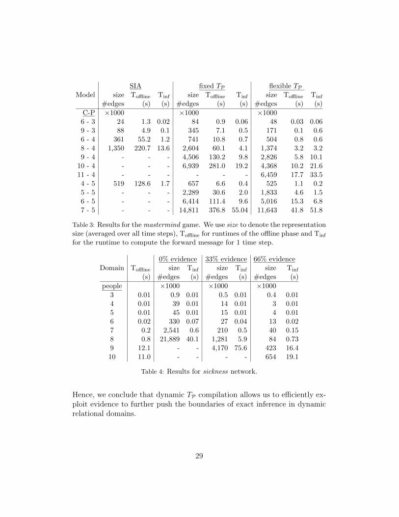
SIA fixed TP flexible TPModel size Toffline Tinf size Toffline Tinf size Toffline Tinf
#edges (s) (s) #edges (s) (s) #edges (s) (s)
C-P ×1000 ×1000 ×10006 - 3 24 1.3 0.02 84 0.9 0.06 48 0.03 0.069 - 3 88 4.9 0.1 345 7.1 0.5 171 0.1 0.66 - 4 361 55.2 1.2 741 10.8 0.7 504 0.8 0.68 - 4 1,350 220.7 13.6 2,604 60.1 4.1 1,374 3.2 3.29 - 4 - - - 4,506 130.2 9.8 2,826 5.8 10.1
10 - 4 - - - 6,939 281.0 19.2 4,368 10.2 21.611 - 4 - - - - - - 6,459 17.7 33.54 - 5 519 128.6 1.7 657 6.6 0.4 525 1.1 0.25 - 5 - - - 2,289 30.6 2.0 1,833 4.6 1.56 - 5 - - - 6,414 111.4 9.6 5,016 15.3 6.87 - 5 - - - 14,811 376.8 55.04 11,643 41.8 51.8
Table 3: Results for the mastermind game. We use size to denote the representationsize (averaged over all time steps), Toffline for runtimes of the offline phase and Tinf
for the runtime to compute the forward message for 1 time step.
0% evidence 33% evidence 66% evidenceDomain Toffline size Tinf size Tinf size Tinf
(s) #edges (s) #edges (s) #edges (s)
people ×1000 ×1000 ×1000
3 0.01 0.9 0.01 0.5 0.01 0.4 0.014 0.01 39 0.01 14 0.01 3 0.015 0.01 45 0.01 15 0.01 4 0.016 0.02 330 0.07 27 0.04 13 0.027 0.2 2,541 0.6 210 0.5 40 0.158 0.8 21,889 40.1 1,281 5.9 84 0.739 12.1 - - 4,170 75.6 423 16.410 11.0 - - - - 654 19.1
Table 4: Results for sickness network.
Hence, we conclude that dynamic TP compilation allows us to efficiently ex-ploit evidence to further push the boundaries of exact inference in dynamicrelational domains.
29
7. Related Work
Knowledge compilation and weighted model counting has shown to bevery effective for inference in probabilistic logic programs (De Raedt et al.,2007; Riguzzi, 2007; Riguzzi and Swift, 2011; Fierens et al., 2015) as wellas graphical models (Chavira and Darwiche, 2005; Darwiche, 2009; Choi etal., 2013). Exact compilation of a propositional formula is computationalexpensive, however, and one often has to resort to approximate techniques.One way to do so is to first convert the program into a propositional formula,as done for exact compilation, but then only compile selected subformulas(Renkens et al., 2014) or feed the formula to a sampling algorithm, e.g. MC-SAT (Poon and Domingos, 2006).
In case also construction of the complete propositional formula becomesinfeasible, one can transform the original program to an approximate, sim-plified program that represents, ideally, a similar probability distribution(Renkens et al., 2012). Other approaches employ forward reasoning to di-rectly sample on the logic program, e.g., (Milch et al., 2005; Goodman etal., 2008; Gutmann et al., 2011; Nitti et al., 2014), but these do not provideguaranteed lower or upper bounds on the probability of the queries. AnytimePLP algorithms based on backward reasoning have been proposed in the pastbut they do not allow to answer multiple queries in parallel (Poole, 1993; DeRaedt et al., 2007). The problem of highly cyclic domains has recently alsobeen addressed using lazy clause generation (Aziz et al., 2015), but only forexact inference.
Probabilistic logic programs under the distribution semantics define adistribution over possible worlds, which randomly fixes the truth values ofprobabilistic facts and then permits any type of logical reasoning within apossible world. While our approach focusses on stratified programs with finitesupport, the fixpoint operator is more recently also extended towards generalnormal programs with function symbols (Bogaerts and Van den Broeck, 2015;Riguzzi, 2016). A second class of probabilistic Prologs, including StochasticLogic Programs (SLPs) (Muggleton, 1996), uses a different approach, where adistribution over the groundings of a query is defined based on a distributionover the derivations in the query’s SLD tree, making an independent decisionon which branch to take at every node. The semantics is thus closely tiedto backward reasoning, and our forward reasoning based approach does noteasily apply in this setting.
Dynamic programs in PLP, one of the use cases considered in this paper,
30
are typically handled by dedicated methods that are extensions of existinginference techniques. Currently, inference in dynamic relational domainsrelies on approximate techniques (de Salvo Braz et al., 2008; Nitti et al., 2013)or requires that each rule in the program considers a transition over time steps(Thon et al., 2011). Other approaches focus on models that are acyclic orpropositional (Murphy, 2002; Sato, 1995; Vlasselaer et al., 2016). Online ordynamic inference has also been considered in the context of Markov logicnetworks, but this only with approximate inference, e.g. (Kersting et al.,2009; Geier and Biundo, 2011).
8. Conclusions
We have introduced TP-compilation, a novel anytime inference approachfor probabilistic logic programs that combines the advantages of forward rea-soning with state-of-the-art techniques for weighted model counting. Our ex-tensive experimental evaluation demonstrates that the new technique outper-forms existing exact and approximate techniques on real-world applicationssuch as biological and social networks and web-page classification. Further-more, we have extended TP-compilation towards dynamic domains and haveshown that it efficiently exploits given observations to scale-up inference.
Acknowledgments
We wish to thank Bart Bogaerts for useful discussions and Adnan Dar-wiche and Arthur Choi for support with the SDD package. Jonas Vlasselaeris supported by IWT (agency for Innovation by Science and Technology).Angelika Kimmig is supported by FWO (Research Foundation-Flanders).
References
Rehan Abdul Aziz, Geoffrey Chu, Christian Muise, and Peter J. Stuckey. StableModel Counting and Its Application in Probabilistic Logic Programming. InProceedings of the 29th AAAI Conference on Artificial Intelligence (AAAI),2015.
Bart Bogaerts and Guy Van den Broeck. Knowledge compilation of logic programsusing approximation fixpoint theory. Theory and Practice of Logic Programming,15(4-5):464–480, 2015.
31
X. Boyen and D. Koller. Tractable Inference for Complex Stochastic Processes. InIn Proceedings of the 14th Conference on Uncertainty in Artificial Intelligence(UAI), 1998.
Mark Chavira and Adnan Darwiche. Compiling Bayesian Networks with LocalStructure. In In Proceedings of the 19th International Joint Conference onArtificial Intelligence (IJCAI), 2005.
Mark Chavira and Adnan Darwiche. On probabilistic inference by weighted modelcounting. Artif. Intell., 172(6-7):772–799, 2008.
Mark Chavira, Adnan Darwiche, and Manfred Jaeger. Compiling relationalBayesian networks for exact inference. International Journal of ApproximateReasoning, 42(1):4–20, 2006.
Arthur Choi, Doga Kisa, and Adnan Darwiche. Compiling Probabilistic GraphicalModels using Sentential Decision Diagrams. In Proceedings of the 12th Euro-pean Conference on Symbolic and Quantitative Approaches to Reasoning withUncertainty (ECSQARU), 2013.
Keith L Clark. Negation as failure. Logic and databases, pages 293–322, 1978.
Adnan Darwiche and Pierre Marquis. A knowledge compilation map. Journal ofAI Research, 17:229–264, 2002.
Adnan Darwiche. New Advances in Compiling CNF into Decomposable NegationNormal Form. In Proceedings of the 16th European Conference on ArtificialIntelligence (ECAI), 2004.
Adnan Darwiche. Modeling and Reasoning with Bayesian Networks. CambridgeUniversity Press, 2009.
Adnan Darwiche. SDD: A New Canonical Representation of Propositional Knowl-edge Bases. In Proceedings of the 22nd International Joint Conference on Arti-ficial Intelligence (IJCAI), 2011.
Jesse Davis and Pedro Domingos. Deep Transfer via Second-Order MarkovLogic. In Proceedings of the 26th International Conference on Machine Learning(ICML), 2009.
Luc De Raedt and Angelika Kimmig. Probabilistic (logic) programming concepts.Machine Learning, 100(1):5–47, 2015.
32
Luc De Raedt, Angelika Kimmig, and Hannu Toivonen. ProbLog: A Probabilis-tic Prolog and Its Application in Link Discovery. In Proceedings of the 20thInternational Joint Conference on Artificial Intelligence (IJCAI), 2007.
L. De Raedt, P. Frasconi, K. Kersting, and S. Muggleton, editors. Probabilistic In-ductive Logic Programming — Theory and Applications, volume 4911 of LectureNotes in Artificial Intelligence. Springer, 2008.
Rodrigo de Salvo Braz, Nimar Arora, Erik Sudderth, and Stuart Russell. Open-universe state estimation with dblog. In NIPS 2008 Workshop, 2008.
Daan Fierens, Guy Van den Broeck, Joris Renkens, Dimitar Shterionov, BerndGutmann, Ingo Thon, Gerda Janssens, and Luc De Raedt. Inference and learn-ing in probabilistic logic programs using weighted Boolean formulas. Theoryand Practice of Logic Programming, 15(03):358–401, May 2015.
Thomas Geier and Susanne Biundo. Approximate Online Inference for DynamicMarkov Logic Networks. In Proceedings of the 23rd International Conferenceon Tools with Artificial Intelligence (ICTAI), 2011.
L. Getoor and B. Taskar, editors. An Introduction to Statistical Relational Learn-ing. MIT Press, 2007.
Noah D. Goodman, Vikash K. Mansinghka, Daniel M. Roy, Keith Bonawitz, andJoshua B. Tenenbaum. Church: a language for generative models. In Proceedingsof the 24th Conference in Uncertainty in Artificial Intelligence (UAI), 2008.
Bernd Gutmann, Ingo Thon, Angelika Kimmig, Maurice Bruynooghe, and Luc DeRaedt. The magic of logical inference in probabilistic programming. Theory andPractice of Logic Programming, 11:663–680, 2011.
Kristian Kersting, Babak Ahmadi, and Sriraam Natarajan. Counting Belief Prop-agation. In Proceedings of the 25th Conference on Uncertainty in ArtificialIntelligence (UAI), 2009.
Brian Milch, Bhaskara Marthi, Stuart J. Russell, David Sontag, Daniel L. Ong,and Andrey Kolobov. BLOG: Probabilistic Models with Unknown Objects. InProceedings of the 19th International Joint Conference on Artificial Intelligence(IJCAI), 2005.
S. H Muggleton. Stochastic logic programs. In L. De Raedt, editor, Advances inInductive Logic Programming, pages 254–264. IOS Press, 1996.
33
Kevin Murphy. Dynamic Bayesian Networks: Representation, Inference andLearning. PhD thesis, UC Berkeley, Computer Science Division, July 2002.
Ulf Nilsson and Jan Maluszynski. Logic, Programming, and PROLOG. John Wiley& Sons, Inc., New York, NY, USA, 2nd edition, 1995.
Davide Nitti, Tinne De Laet, and Luc De Raedt. A particle filter for hybridrelational domains. In IEEE/RSJ International Conference on Intelligent Robotsand Systems (IROS), 2013.
Davide Nitti, Tinne De Laet, and Luc De Raedt. Relational object trackingand learning. In IEEE International Conference on Robotics and Automation(ICRA), 2014.
Oved Ourfali, Tomer Shlomi, Trey Ideker, Eytan Ruppin, and Roded Sharan.SPINE: a framework for signaling-regulatory pathway inference from cause-effect experiments. Bioinformatics, 23(13):359–366, 2007.
Avi Pfeffer. Practical Probabilistic Programming. Manning Publications, 2014.
David Poole. Logic programming, abduction and probability. New GenerationComputing, 11:377–400, 1993.
Hoifung Poon and Pedro Domingos. Sound and Efficient Inference with Proba-bilistic and Deterministic Dependencies. In Proceedings of the 21st NationalConference on Artificial Intelligence (AAAI), 2006.
Joris Renkens, Guy Van den Broeck, and Siegfried Nijssen. k-optimal: A novelapproximate inference algorithm for ProbLog. Machine Learning, 89(3):215–231, 2012.
Joris Renkens, Angelika Kimmig, Guy Van den Broeck, and Luc De Raedt.Explanation-based approximate weighted model counting for probabilistic log-ics. In Proceedings of the 28th AAAI Conference on Artificial Intelligence(AAAI), 2014.
Fabrizio Riguzzi and Terrance Swift. The PITA System: Tabling and AnswerSubsumption for Reasoning under Uncertainty. Theory and Practice of LogicProgramming, 11(4–5):433–449, 2011.
Fabrizio Riguzzi. A Top Down Interpreter for LPAD and CP-Logic. In Proceed-ings of the 10th Congress of the Italian Association for Artificial Intelligence(AI*IA), 2007.
34
Fabrizio Riguzzi. The Distribution Semantics for Normal Programs with FunctionSymbols. International Journal of Approximate Reasoning (Special Issue onProbabilistic Logic Programming), (Accepted), 2016.
Taisuke Sato. A statistical learning method for logic programs with distributionsemantics. In Proceedings of the 12th International Conference on Logic Pro-gramming (ICLP), 1995.
Dan Suciu, Dan Olteanu, R. Christopher, and Christoph Koch. ProbabilisticDatabases. Morgan & Claypool Publishers, 1st edition, 2011.
Ingo Thon, Landwehr Niels, and Luc De Raedt. Stochastic relational processes:Efficient inference and applications. Machine Learning, 82(2):239–272, February2011.
Guy Van den Broeck and Adnan Darwiche. On the Role of Canonicity in Knowl-edge Compilation. In Proceedings of the 29th Conference on Artificial Intelli-gence (AAAI), 2015.
Maarten. H. Van Emden and Robert. A. Kowalski. The Semantics of PredicateLogic as a Programming Language. Journal of the ACM, 23:569–574, 1976.
Allen Van Gelder, Kenneth A. Ross, and John S. Schlipf. The Well-founded Se-mantics for General Logic Programs. J. ACM, 38(3):619–649, July 1991.
Joost Vennekens, Sofie Verbaeten, and Maurice Bruynooghe. Logic programs withannotated disjunctions. In Proceedings of the 20th International Conference onLogic Programming (ICLP), 2004.
Joost Vennekens, Marc Denecker, and Maurice Bruynooghe. CP-logic: A languageof causal probabilistic events and its relation to logic programming. Theory andPractice of Logic Programming, 9(3), 2009.
Jonas Vlasselaer, Guy Van den Broeck, Angelika Kimmig, Wannes Meert, andLuc De Raedt. Anytime inference in probabilistic logic programs with Tp-compilation. In Proceedings of 24th International Joint Conference on ArtificialIntelligence (IJCAI), July 2015.
Jonas Vlasselaer, Wannes Meert, Guy Van den Broeck, and Luc De Raedt. Ex-ploiting local and repeated structure in dynamic Bayesian networks. ArtificialIntelligence, 232:43–53, March 2016.
35