T C N

Help

Notes

• Bullets Math  text

Although any given solution to an NP-complete problem can be verified quickly (in polynomial time), there is no known efficient way to locate a solution in the first place; indeed, the most notable characteristic of NP-complete problems is that no fast solution to them is known. That is, the time required to solve the problem using any currently known algorithm increases very quickly as the size of the problem grows. This means that the time required to solve even moderately sized versions of many of these problems can easily reach into the billions or trillions of years, using any amount of computing power available today. As a consequence, determining whether or not it is possible to solve these problems quickly, called the P versus NP problem, is one of the principal unsolved problems in computer science today. http://en.wikipedia.org/wiki/NP-complete

An algorithm is said to take superpolynomial time if T(n) is not bounded above by any polynomial. It is ω(nc) time for all constants c, where n is the input parameter, typically the number of bits in the input.

For example, an algorithm that runs for 2n steps on an input of size n requires superpolynomial time (more specifically, exponential time).

An algorithm that uses exponential resources is clearly superpolynomial, but some algorithms are only very weakly superpolynomial. For example, the Adleman–Pomerance–Rumely primality test runs for nO(log log n) time on n-bit inputs; this grows faster than any polynomial for large enough n, but the input size must become impractically large before it cannot be dominated by a polynomial with small degree.

An algorithm that requires superpolynomial time lies outside the complexity class P. Cobham's thesis posits that these algorithms are impractical, and in many cases they are. Since the P versus NP problem is unresolved, no algorithm for an NP-complete problem is currently known to run in polynomial time .http://en.wikipedia.org/wiki/Superpolynomial#Superpolynomial_time

2016Reinstate traveling salesman problem

• Based on Chap. 6 of Aleksander and Morton• Hopfield and Tank (1985)• Hopfield and Tank (1986) // minor• Bits from Haykin. // minor

20152016: Reinstate traveling salesman problem

Review: Dark Age of neural computation

• Key I-O functions require multilayer perceptrons• Absence of appropriate learning rules

Linear threshold neurons

(McCullough-Pitts, 1943)

Synaptic learning rules,

unsupervised (Hebb, 1949)

Perceptron convergence

proof (Novikoff, 1962)

Perceptrons defined

(Roseblatt, 1962)

Synaptic learning rules,

supervised (Widrow, 1962)

Autoassociative networks

(Hopfield, 1982)

Limitations on perceptron

learning (Minksy & Papert, 1969)

Boltzmann machine learning (Hinton,

Sejnowski, Ackeley, 1984)

Backpropagation, perceptron

limitation overcome (Rumelhart,

Hinton, Williams, 1986)

NetTalk

(Sejnowski &

Rosenburg, 1987)

Image compression

(Cottrell, Munro,

Zipser, 1987)

Backprop. net predicts cortical

receptive fields

(Zipser & Andersen, 1988)

Two main events ended the Dark Age of neural computation

o Hopfield networks (1982) // Showed the interesting problems could be computed and learned; got physicists interested

o Backpropagation (1986)* // Generalized the perceptron learning rule to multiple layers

* Werbos (1974)

Comparison of Hopfield networks and perceptrons

Same

o McCullough-Pitt neurons (Net input, threshold, 0/1 output)o Trainable

Different

o No layerso Every neuron is both an input and an output neurono Full connectivity*, hence feedbacko Constraints on weights (symmetry)o Asynchronous updating (due to feedback connections)o Compute by relaxation to stable states

Stable states can be established by training or engineering (from first principles)

* Except self connections

Perceptron

Hopfield network

Wij  =  Wji

NotationVi  :  Current  state  of  neuron  i  

       Vi’  :  Next  state  of  neuron  i     Ui  :  Threshold  of  neuron  i     Wij  or  Tij  :  Connection  strength  from  i  to  j     Ni  :  Net  input  to  i,  Ni  =  Sum_j[Wji]  *  Vj     F(N,U)  =  Perceptron  nonlinearity  

Randomly pick one neuron to update P  =  1/3

If  Unit  1:  N1  =  W21  V2  +  W31  V3  =  0  +  0  V1’  =  F(N1,  U1)  =  F(0,  0.7)  =>  OFF  

If  Unit  2:  N1  =  W12  V1  +  W32  V3  =  0.5  +  0  V2’  =  F(N2,  U2)  =  F(0.5,  -­‐0.2)  =>  ON  

If  Unit  3:  N3  =  W13  V1  +  W23  V2  =  0.4  V2’  =  F(N3,  U3)  =  F(0.4,  0.4)  =>  OFF  

Repeat…  

How a Hopfield network is simulated

Unit  2  picked      (1/3)

Unit  3  picked    (1/3)

Unit  1  picked    (1/3)

Network

State transition diagram

1

2 3

1

2 3

1

2 3

U1 = 0.7

How a Hopfield network is analyzed

Case  1    (1/3)

Case  2    (1/3)

Case  3    (1/3)

State transition diagram

P  =  0.5 P  =  0.5

Fate diagramWhen it leaves, where does it go?

How a Hopfield network is analyzed

Example:  P(A|c),  P(B|c)

State transition diagram Conversion rules

Homework problem…A is a stable state

1/3 1/3 1/3

1/3

1/3 1/3 1/2 1/2

2/3

1/3 1

3/3

0

1/3 1/3 1/3

⇒

⇒

⇒

⇒

Transitionprobs

Fateprobs

How a Hopfield network is analyzedState transition diagram

A is a stable state

⇒ State transition diagramFate diagram

1/3

1/3

1/3

1/2

1/2

1/21/2

1/2

1/2

1/2

1/2

1 0

0

Fate probabilities

State transition diagramFate diagram

1/3

1/3

1/3

1/2

1/2

1/21/2

1/2

1/2

1/2

1/2

1 0

0

Hopfield networks compute by relaxation to stable states

Example  Input  (0,0,1)  =  State  c

P(c-e-A) = 1/2 · 1 = 1/2

P(c-d-A) = 1/2 · 1/2 = 1/4

P(c-d-B) = 1/2 · 1/2 = 1/4

Input P(A)c

P(B)3/4 1/4

Tabulation

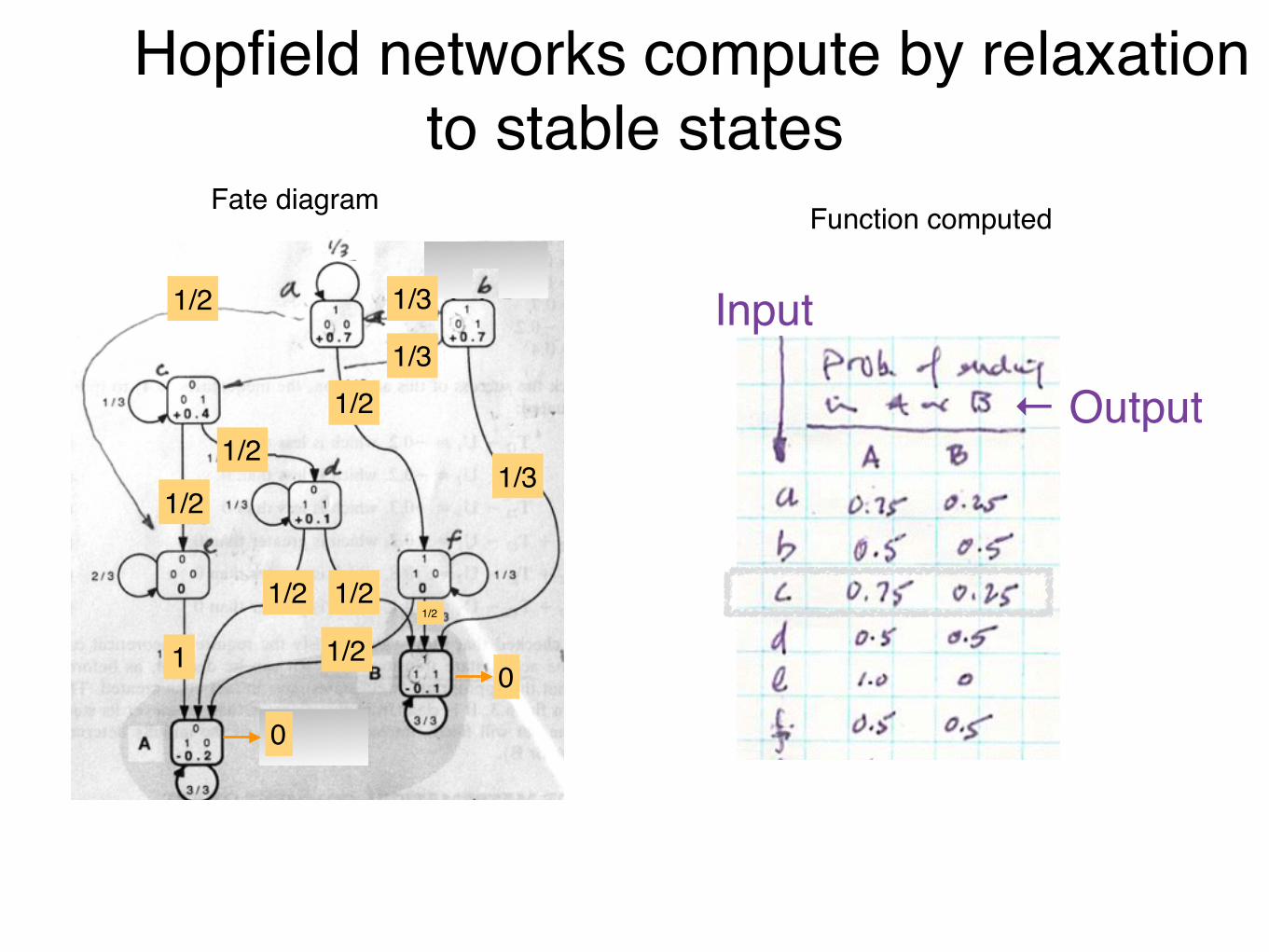
Hopfield networks compute by relaxation to stable states

Function computed

Input

← Output

State transition diagramFate diagram

1/3

1/3

1/3

1/2

1/2

1/21/2

1/2

1/2

1/2

1/2

1 0

0

Stable states can be trained or engineered

Either method is best understood in terms of the network’s Hopfield energy E.

Hopfield energy EE = U1 V1 + U2 V2 + U3 V3 - (T12 V1 V2 + T13 V1 V3 + T23 V2 V3)

Why this definition of E?

When a unit changes state:

∆E = En+1 - En

Plug E into this equation, get

∆E = - ∆Vi (Ni - Ui)

2 3

1

1

2 3

En+1

En

Logic:

Units in the “wrong” state have high E

Case I: Unit i is off but should be on

(Ni - Ui) > 0 // Unit above threshold∆Vi > 0

Case II: Unit is on but should be off

(Ni - Ui) < 0 // Unit below threshold∆Vi < 0

So energy ∆E is negative: energy is released when units (correctly) change state

Instructor notes (replace)Notation (suppressing subscript i)

V  :  State  of  neuron  i     U  :  Threshold  of  neuron  i     N  :  Net  input  to  i

Definition       ∆E  =  -­‐V  *  (N  -­‐  U)  

Comments

E can be positive or negative

E = 0 for neurons that are off (V  =  0)

E  changes iff V  changes (because N  -­‐  U is constant)

Neurons in the wrong state* are at higher E** than they should be (“tense”)

Neurons in the correct state* are at lower E than if they changed state (“relaxed”)

* Based on N  vs  U     ** Even if their energy is zero

WRONG(SEE NEXT SLIDE)

Stable states can be established by trainingApply the “delta rule”Example: (0,1,0) as target stable stateStart with arbitrary W and U

DoCompute V1,  V2,  V3  

  For each neuron iCompare Vi to the target value (0,1,0)If Vi = target, to nothingIf Vi is too high, decrease active Ws and increase active Us if Vi is too low, do the opposite

end forWhile(the pattern is not = A)

The delta rule works because it minimizes Hopfield energy by driving W and U to maximally relaxed configurations

Content addressable memoryHopfield network

Fundamental memories Recall

Stable states can be established by engineering from first principles

Example: the Traveling Salesman Problem (TSP)

Find the shortest path connecting n cities, visiting each on only once

Computational time grows exponentially with n

Drawbacks of Hopfield networks

False energy minima

Low storage capacity: number of patterns = n

Does not solve the problem of hard learninge.g. parity

FIX: Probabilistic neurons (Boltzmann machines)

Hopfield network

Hopfield network solution to the TSP

Example: the Traveling Salesman Problem

Find the shortest path connecting n cities, visiting each on only once

Computational time grows exponentially with n

Network-level representation

HopMield  and  Tank  1985

How the network was engineered

Notation : V is state, X is row (city), Y is column (visit rank)

Term 1 : Zero IFF one city per rowTerm 2 : Zero IFF one city per columnTerm 3 : Zero IFF n neurons are ONTerm 4 : Bias toward short tours

Method: randomize the starting state as seewhere the network stabilizes. Each stable point is a potential solution.

+

HopMield  and  Tank  1985

with

X

Y

Add picture of route

2010

• Bullets Math  text

Instantaneous neurons in feedback networks

1. Hopfield networks and content addressable memory

2. Analysis methods for Hopfield networks

• Bullets Math  text

Early history of nervous system models

Linear threshold neurons

(McCullough-Pitts, 1943)

Synaptic learning rules,

unsupervised (Hebb, 1949)

Perceptron convergence

proof (Novikoff, 1962)

Perceptrons defined

(Roseblatt, 1962)

Synaptic learning rules,

supervised (Widrow, 1962)

Autoassociative networks

(Hopfield, 1982)

Limitations on perceptron

learning (Minksy & Papert, 1969)

Boltzmann machine learning (Hinton,

Sejnowski, Ackeley, 1984)

Backpropagation, perceptron

limitation overcome (Rumelhart,

Hinton, Williams, 1986)

NetTalk

(Sejnowski &

Rosenburg, 1987)

Image compression

(Cottrell, Munro,

Zipser, 1987)

Backprop. net predicts cortical

receptive fields

(Zipser & Andersen, 1988)

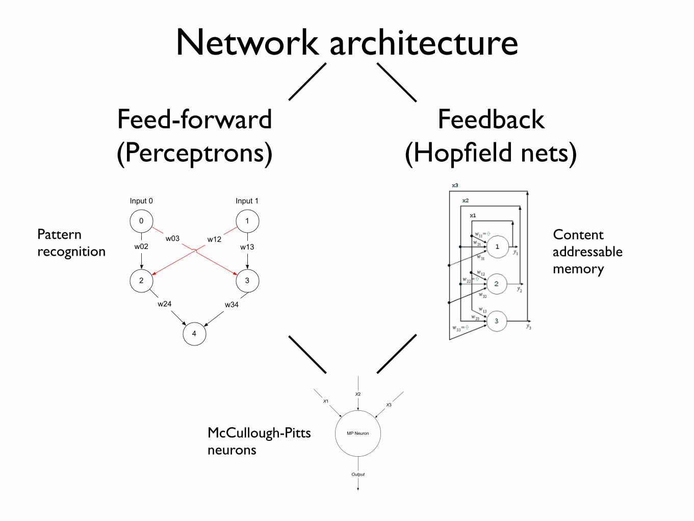
Network architecture

Feed-forward(Perceptrons)

Feedback(Hopfield nets)

0 1

2 3

4

Input 1Input 0

w02 w13w12w03

w24 w34

Patternrecognition

Content addressablememory

MP Neuron

X1

X2

X3

Output

McCullough-Pittsneurons

Content addressable memoryHopfield network

Mistakes

Wrong fundamental memories Spurious stable states

Lab exercise: toy Hopfield network

b

B

d

A

Stimulus

Recall

Feedback networks + instantaneous neurons = update problem

“Updating a neuron’s state updates its input, hence it’s state, hence its input...”

Solution: asynchronous updating

Neuron 0

Neuron 2Neuron 1

State transition map(1) Determine which neurons, when chosen to update do, and do not, change their activation

(2) Find neighboring states

Example: state e

NeuronCurrent state

W * state of neuron #1W * state of neuron #2

Sum of inputs (N)Threshold (U)

Updated state

NeuronActivity (A)

InputInput

Sum of inputs (N)Threshold (U)

Activity (A’)Next state

NeuronActivity (A)

InputInput

Sum of inputs (N)Threshold (U)

Activity (A’)Next state

End-state probabilities

Example: state c

Path 1: Prob(c-a-A) = (0.5)(1.0) = 0.5

Path 2: Prob(c-e-A) = ( )( ) =

Path 3: Prob(c-e-B) = ( )( ) =

Homework

Homework

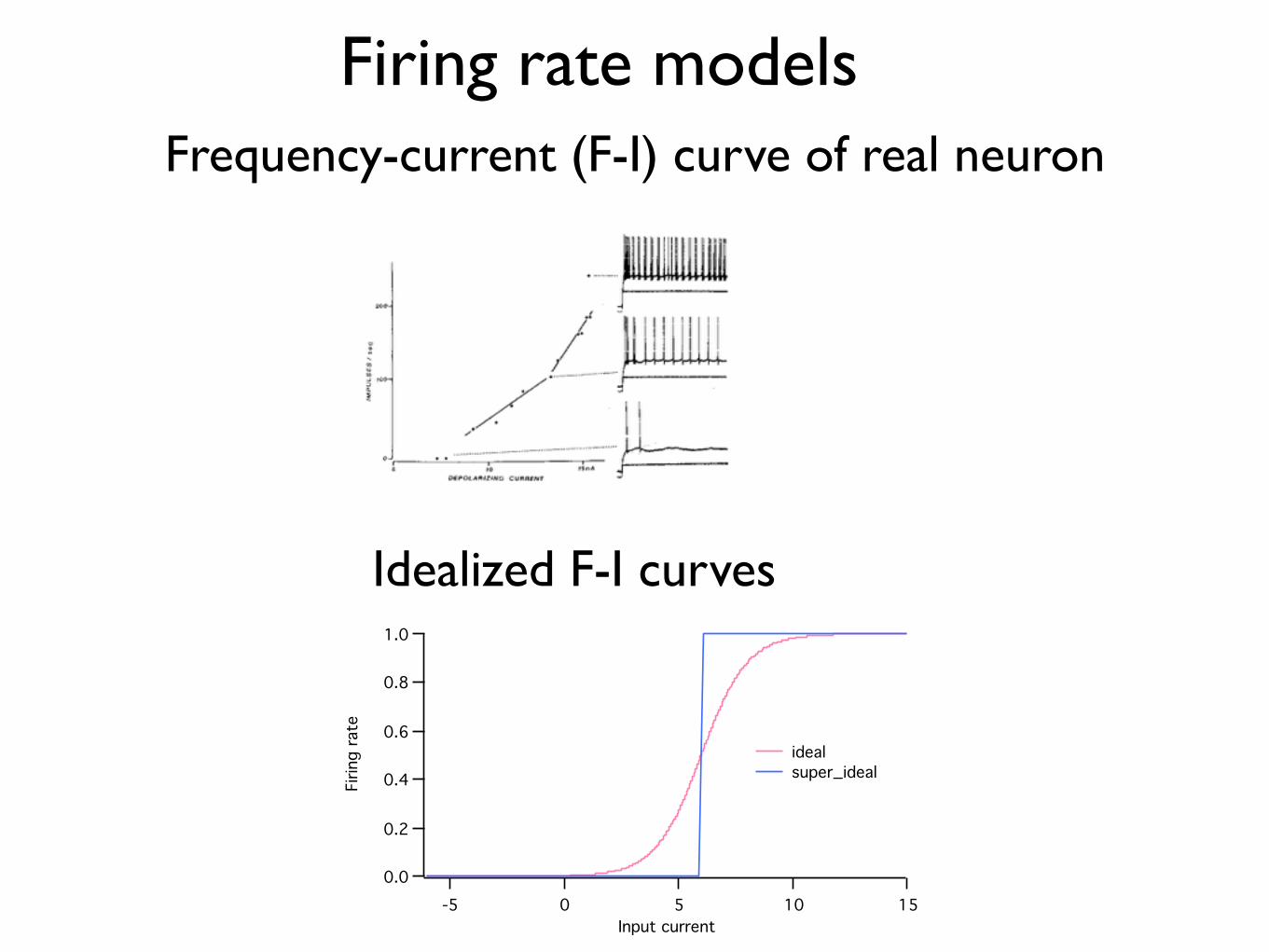
Firing rate modelsFrequency-current (F-I) curve of real neuron

Idealized F-I curves1.0

0.8

0.6

0.4

0.2

0.0

Firin

g r

ate

151050-5

Input current

ideal

super_ideal