systems with more than one unpaired electron

CHAPTER 6

SYSTEMS WITH MORE THAN ONEUNPAIRED ELECTRON

6.1 INTRODUCTION

Nearly all the species considered in previous chapters had only one unpaired

electron (viz., S ¼ 12). In principle, an EPR spectrum is obtainable for any system

with an odd number of electrons (S ¼ 12, 3

2, 5

2, . . .). For systems with an even

number of electrons (S ¼ 1, 2, 3, . . . ), there is no such guarantee; however, as we

shall see, many systems of the latter type are accessible to EPR spectroscopy.

We begin by considering the theory of systems with two unpaired electrons,

initially ignoring all nuclear spins.1 Such systems include (1) atoms or ions in the

gas phase (e.g., oxygen atoms), (2) small molecules in the gas phase (e.g., O2),

(3) organic molecules containing two or more unpaired electrons (e.g., naphthalene

excited to its metastable triplet state) in solid-state solutions and crystals, (4) inor-

ganic molecules (e.g., CCO in rare-gas matrices), (5) ‘point’ defects in crystals con-

taining more than one unpaired electron (e.g., the Ft center in MgO), (6) biradicals in

fluid solution and the solid state and (7) certain transition-group (e.g., V3þ and Ni2þ)

and rare-earth ions. Systems 1 and 2 are dealt with in Chapter 7.

In all chemical species, if the highest occupied electronic level is orbitally non-

degenerate and is doubly occupied by electrons, the ground state must be a spin

singlet (Fig. 6.1a). If one of these electrons is excited to an unoccupied orbital by

absorption of a quantum of the appropriate energy (Fig. 6.1b), the system is still

in a singlet state, since allowed transitions occur without change of multiplicity.

However, the molecule may then undergo intersystem crossing to a metastable

triplet state, with a change of spin (Fig. 6.1c). This process is attributed to the

158

Electron Paramagnetic Resonance, Second Edition, by John A. Weil and James R. BoltonCopyright # 2007 John Wiley & Sons, Inc.

presence of spin-orbit coupling, molecular rotation and/or hyperfine interaction in

the presence of an external field B. It is highly selective in populating the three sub-

levels; that is, the process leads to spin polarization.

A triplet ground state (Fig. 6.1d ) requires, in view of the Pauli exclusion principle

[1], that this state have at least a two-fold orbital degeneracy (or near degeneracy).

Low-lying orbitals filled with electrons have been shown in Fig. 6.1 to emphasize

that it is the set of highest occupied orbitals that is important in determining the

multiplicity of the state.

6.2 SPIN HAMILTONIAN FOR TWO INTERACTING ELECTRONS

For the case of two electrons there are four spin states. One way of representing these

states is to construct simple product spin states (the uncoupled representation;

Section B.6)

a(1)a(2) a(1)b(2) b(1)a(2) b(1)b(2) Set (6:1)

In a paramagnetic center of moderate size, such that the two electrons interact

appreciably, it is more advantageous to combine these configurations into combi-

nation states (the coupled representation) because the system separates in energy

FIGURE 6.1 Energy levels and spin configuration of a six-electron system in: (a) its

singlet ground state; (b) after electronic excitation (the spins remain paired and hence

the state is a singlet); (c) after the molecule goes to a metastable triplet state via a

radiationless process (the triplet state is usually lower in energy than the singlet state

[in (b)] because of decreased interelectronic repulsion); and (d ) configuration of a

four-electron system with a triplet ground state. The lowest level is symbolic of filled

orbitals below the degenerate pair; it is irrelevant whether the filled orbitals are

degenerate or non-degenerate.

6.2 SPIN HAMILTONIAN FOR TWO INTERACTING ELECTRONS 159

into a triplet state and a singlet state.2 These coupled functions are either symmetric

or antisymmetric with respect to exchange of the electrons. The combination func-

tions are (Section B.6)

Symmetric Antisymmetric

a(1)a(2)1ffiffiffi

2p a(1)b(2)þ b(1)a(2)½ �

1ffiffiffi

2p a(1)b(2)� b(1)a(2)½ �

b(1)b(2)

Triplet state, S ¼ 1 Singlet state, S ¼ 0

Set (6:2)

The multiplicity of the state with total spin S ¼ 1 is 2Sþ 1 ¼ 3; hence it is called a

triplet state. The state with S ¼ 0 analogously is called a singlet state. If the two

electrons occupy the same spatial orbital, then only the antisymmetric or singlet

state is possible because of the restrictions imposed by the Pauli exclusion principle

[1]. However, if each electron occupies a different orbital, then both the singlet and

triplet states exist.3

6.2.1 Electron-Exchange Interaction

The singlet and triplet states are split apart in energy by the electron-exchange inter-

action, represented by the spin hamiltonian

Hexch ¼X

ij

JijS1iS2j (i, j ¼ 1, 2, 3) (6:3a)

¼ 12

(S1T� J � S2 þ S2

T� JT� S1) (6:3b)

where S1 and S2 are the electron-spin operators for electrons 1 and 2 (Section B.10

and Problem B.11). Indices i and j label spatial coordinates.

Here J is a 3 � 3 matrix that takes into account the electric (coulombic) inter-

action between the two unpaired electrons, but not the important magnetic inter-

action that is introduced in Section 6.2.2. Details concerning the theory of

exchange-coupled systems are available in the literature [2–4].

For our purposes, we consider only the most important part of the exchange-

energy operator (Eq. 6.3), that is, the isotropic part4

Hexch

� �

iso¼ J0 S1

T� S2 (6:4)

where J0 ¼ tr(J)/3 is the isotropic electron-exchange coupling constant, which to a

first approximation is given [5] by the exchange integral

J0 ¼ �2�

fa(1)fb(2)je2

4p10rjfa(2)fb(1)

�

(6:5)

Here fa and fb are different normalized spatial molecular-orbital wavefunctions,

evaluated while considering the electrons to be non-interacting, 10 is the permittivity

160 SYSTEMS WITH MORE THAN ONE UNPAIRED ELECTRON

of the vacuum, and r is the inter-electron distance.5 Whether the singlet or the triplet

state lies lower depends on the sign of J0. The interaction between two hydrogen

atoms is a textbook example; here J0 . 0 and the singlet (bonding) state lies

lowest. In the molecular-orbital description of H2, J0 is a major contribution to

the total binding energy. If J0 , 0, as is the case in some species, the triplet state

has the lower energy (Fig. 6.2).

In analogy with the isotropic electron-nuclear hyperfine interaction (Eq. C.2b),

Eq. 6.3 can be written as

Hexch

� �

iso¼ J0 ½S1zS2z þ

12

(S1þS2� þ S1�S2þ)� (6:6)

Application of this operator to the spin wavefunctions shows that the singlet and

triplet states are separated by the energy jJ0j (Fig. 6.2), with eigenfunctions as

listed in set 6.2. Experimentally, one can observe which state (the singlet or

triplet) is lower in energy by studying the EPR signal intensity (i.e., the spin-level

populations) as the temperature approaches 0 K.

Note that J0 is the analog of the isotropic hyperfine coupling parameter intro-

duced in Eq. 2.39b. As pointed out, the four energy levels of the hydrogen atom

are similarly split at zero field into a triplet and a singlet (Appendix C). There is

also considerable analogy to the NMR isotropic spin-spin coupling constant J.

The magnitude of J0 decreases with increasing r (Eq. 6.5), so that jJ0j is very

small if the two electrons are on the average sufficiently far apart. In this case, if

the exchange energy is not large compared to the magnetic dipolar interaction

energy, then the two-electron system is called a biradical.

FIGURE 6.2 The state energies of a system of two electrons exhibiting an exchange

interaction, for J0 , 0. When J0 is positive, the singlet state lies lower in energy.


6.2.2 Electron-Electron Dipole Interaction

In addition to electron exchange, which splits the states into a singlet and a triplet,

there exists another important interaction, also quadratic in the electron spin,

namely, the anisotropic magnetic dipole-dipole interaction.6 This interaction

causes the three-fold degeneracy of the triplet state to be removed even in zero mag-

netic field; the latter effect often is called zero-field splitting.7

The dipole-dipole interaction for the coupling of two unpaired electrons is

analogous to the corresponding interaction (Eq. 5.3) between electronic and

nuclear magnetic dipoles, which gives rise to the anisotropic hyperfine interaction

(Fig. 2.2); that is, the electron-spin electron-spin dipolar interaction is given by

the hamiltonian

Hss(r) ¼m0

4p

m1T� m2

r3�

3(m1T� r)(m2

T� r)

r5

� �

(6:7)

Here the inter-electron vector r is defined as in Fig. 2.2 with mn replaced by me. The

magnetic-moment operators may be replaced by the corresponding spin operators, to

yield

Hss(r) ¼m0

4pg1 g2be

2 S1T� S2

r3�

3(S1T� r)(S2

T� r)

r5

" #

(6:8)

where g1 and g2 are the g factors for electrons 1 and 2, taken here to be isotropic.

Henceforth, for simplicity, we assume that g1 ¼ g2 ¼ g. Expansion of the scalar

products in Eq. 6.8 yields

Hss(r) ¼m0

4p

(gbe)2

r5(r2 � 3x2)S1xS2x þ (r2 � 3y2)S1yS2yþ

h

(r2 � 3z2)S1zS2z � 3xy(S1xS2y þ S1yS2x)�

3xz(S1xS2z þ S1zS2x)� 3yz(S1yS2z þ S1zS2y)i

(6:9)

Because the two electrons are coupled, it is more convenient to express Hss in terms

of the total spin operator S, defined by

S ¼ S1 þ S2 (6:10)

This is accomplished by expanding the appropriate operators, for example

Sx2 ¼ (S1x þ S2x)2 ¼ S1x

2 þ S2x2 þ S1xS2x þ S2xS1x (6:11)

Note that S1 and S2 commute since they are operators for different particles. Hence

S1xS2x ¼12Sx

2 � 1413 (6:12)

since the eigenvalues of S1x2 and S2x

2 are both 14

(Section B.6). Similar expressions

are obtained for the y and z terms. An expression for S1T � S2 then follows (note


Eq. B.49). The circumflex about the unit matrix symbol signals that we are dealing

with a three-dimensional quantum-mechanical space (i.e., the spin triplet state),

rather than with ordinary 3-space.

Using the angular-momentum commutation relations (Eqs. B.12), the following

transformation can be derived

S1xS2y þ S2xS1y ¼12

(SxSy þ SySx) (6:13)

with similar expressions for the xz and yz components.

Substitution of these expressions into Eq. 6.9, together with the identity

r2 ¼ x2þ y2þ z2, yields

Hss(r) ¼m0

4p

(gbe)2

r5

1

2(r2 � 3x2)Sx

2 þ (r2 � 3y2)Sy2 þ (r2 � 3z2)Sz

2h

�

3xy(SxSy þ SySx)� 3xz(SxSz þ SzSx)� 3yz(SySz þ SzSy)i

(6:14)

The factor of 12

arises from the conversion from the S1, S2 basis to the S basis.

Because all matrix elements connecting the triplet and singlet manifolds are zero

in Hss(r) as well as in S, one can switch from consideration of the full manifold

to working separately with the triplet and singlet parts. The corresponding dipolar

energy for the latter (S ¼ 0) is, of course, zero.

Equation 6.14 can be converted into a spin-hamiltonian form by suitable

integration; it can then be written more conveniently in matrix form as

Hss¼m0

8p(gbe)2 Sx Sy Sz

h i

�

r2�3x2

r5

�3xy

r5

�3xz

r5

r2�3y2

r5

�3yz

r5

r2�3z2

r5

2

6

6

6

6

6

6

6

6

6

4

3

7

7

7

7

7

7

7

7

7

5

�

Sx

Sy

Sz

2

6

6

6

6

6

6

6

6

6

4

3

7

7

7

7

7

7

7

7

7

5

(6:15a)

¼ ST�D� S for S¼0, 1 (6:15b)

¼ S1T�D� S2þ S2

T�D� S1 (¼ 2S1T�D� S2) (6:15c)

Note that S1T�D� S1 ¼ S2

T�D� S2 ¼ 0. The last form results from the interchange-

ability of the individual spins S1, S2. Operator Hss is sometimes called the ‘electronic

quadrupole spin hamiltonian’. As before, the angular brackets indicate that the

elements of the parameter matrix D are averages over the electronic spatial wavefunc-

tion. As with the matrices encountered in Chapters 4 and 5, D can be diagonalized, to


dD. The diagonal elements of dD are DX, DY and DZ. By convention, DZ is taken to be

the principal value with the largest absolute magnitude and DY has the smallest absol-

ute magnitude when DX = DY, producing a set ordered in energy.

We see from the sum of the diagonal elements of Eq. 6.15a that D is a matrix with

a trace of zero:

tr(D) ¼ DX þ DY þ DZ ¼ 0 (6:16)

In the principal-axis system of D, Eq. 6.15b becomes

Hss ¼ DXSX2 þ DY SY

2 þ DZSZ2 (6:17)

As always, the principal-axis system is defined by the details of the interaction

giving rise to the 3 � 3 matrix. The axes lie on symmetry elements, for example,

along molecular symmetry axes when such are present.

The dipole-dipole coupling between the two unpaired electrons is not the only

interaction that can lead to a spin-hamiltonian term of the form of Eq. 6.15b. Coupling

between the electron spin and the electronic orbital angular momentum (Section 4.8)

gives rise to a term of the same form (Eq. 6.15b), as does the generalized anisotropic

exchange interaction [8].

The effective spin hamiltonian for two interacting electrons, obtained by adding

Eqs. 6.4 and 6.15b to the electron Zeeman term, is

H ¼ gbeBT� Sþ ST�D � Sþ 12

J0 S2 � 32

13

h i

(6:18)

where the form of the last term arises from the vector cosine sum rule (Eq. B.49).

If J0 , 0 and jJ0j .. kbT, only the lower (S ¼ 1) state is populated. Conversely,

if J0 .. kbT, only the diamagnetic (S ¼ 0) state is thermally populated. Furthermore,

since the exchange term of Eq. 6.18 contributes only a common constant to the energy

of each of the three triplet states, it is neglected in the next section.

6.3 SYSTEMS WITH S 5 1 (TRIPLET STATES)

From our previous discussion we see that the spin hamiltonian for an S ¼ 1 state is

H ¼ gbeBT� Sþ ST�D � S (6:19a)

If D is expressed in its principal-axis system, Eq. 6.19a may be written as

H ¼ gbeBT� Sþ DXSX2 þ DY SY

2 þ DZSZ2 (6:19b)


Note that, although there are actually two unpaired electrons (each S ¼ 12) in the

triplet molecule, we use an effective spin S 0 ¼ 1 to describe its magnetic properties,

with the singlet ignored. Thus, while there really are four spin states, only three are

active. The use of an effective spin, one that generates the multiplicity needed for the

states considered, is common and convenient in magnetic resonance. For one, it

allows a simple formulation of the spin hamiltonian describing the system.

6.3.1 Spin Energies and Eigenfunctions

It is often convenient to use the eigenfunctions jMSl ¼ jþ1l, j0l and j–1l of SZ as

a basis set (Fig. 6.2); these are the eigenfunctions of H (Eq. 6.19b) in the limit as

B! 0. However, they are not eigenfunctions of H ss (Eqs. 6.15b and 6.17).

Hence it is necessary to set up the spin-hamiltonian matrix for H and find its

energy eigenvalues and eigenstates. For present purposes, it is not necessary to

know how the principal-axis system is oriented but only that it exists. Equation

6.19b can be written as

H ¼ gbe(BXSX þ BY SY þ BZSZ)þ DXSX2 þ DY SY

2 þ DZSZ2 (6:19c)

If we take the quantization axis for S along principal axis Z, then the required spin

matrices are those given in Eq. B.77. Substitution of these into Eq. 6.19c with sub-

sequent matrix addition and multiplication yields spin-hamiltonian matrix

jþ1i j0i j�1i

H ¼

hþ1j

h0j

h�1j

gbeBZ þ1

3D

1ffiffiffi

2p gbe(BX � iBY )

1

2(DX � DY )

1ffiffiffi

2p gbe(BX þ iBY ) DX þ DY

1ffiffiffi

2p gbe(BX � iBY )

1

2(DX � DY )

1ffiffiffi

2p gbe(BX þ iBY ) �gbeBZ þ

1

3D

2

6

6

6

6

6

6

4

3

7

7

7

7

7

7

5

(6:20)

where D/3 ¼ (DXþDY)/2þDZ. The secular determinant (Eq. A.69a) is obtained

fromH by subtracting energy U from all diagonal elements. Setting the correspond-

ing determinant equal to zero, one obtains

gbeBZ þ1

2DZ � U

1ffiffiffi

2p gbe(BX � iBY )

1

2(DX � DY )

1ffiffiffi

2p gbe(BX þ iBY ) �DZ � U

1ffiffiffi

2p gbe(BX � iBY )

1

2(DX � DY )

1ffiffiffi

2p gbe(BX þ iBY ) �gbeBZ þ

1

2DZ � U

�

�

�

�

�

�

�

�

�

�

�

�

�

�

�

�

�

�

�

�

�

�

�

�

¼ 0 (6:21)

6.3 SYSTEMS WITH S ¼ 1 165

Here Eq. 6.16 has been used to simplify terms. The situation is especially simple

when B k Z. Then BX ¼ BY ¼ 0, and Eq. 6.21 becomes

gbeBZ þ1

2DZ � U 0

1

2(DX � DY )

0 �DZ � U 0

1

2(DX � DY ) 0 �gbeBZ þ

1

2DZ � U

�

�

�

�

�

�

�

�

�

�

�

�

�

�

�

�

�

�

�

�

¼ 0 (6:22)

The solution U ¼ –DZ is obtained by inspection. Expansion of the remaining 2 � 2

determinant gives the other two energies as

UX,Y ¼12

{DZ + ½4g2be2BZ

2 þ (DX � DY )2�1=2} (6:23)

In zero magnetic field, the energies are

UX ¼12½DZ � (DX � DY )� ¼ �DX (6:24a)

UY ¼12½DZ þ (DX � DY )� ¼ �DY (6:24b)

UZ ¼ �DZ (6:24c)

Thus jUZj . jUXj � jUYj at B ¼ 0, in accordance with our convention (Section

6.2.2). We note that the zero in energy lies between the smallest and the largest

principal D values, and that all the degeneracy is removed except in the uniaxial

case. In the literature, the notation x ¼ 2DX, Y ¼ 2DY and Z ¼ 2DZ has some-

times been used.

Since the trace of D is zero, only two independent energy parameters are required.

It is common to designate these as

D ¼ 32

DZ (6:25a)

E ¼ 12

(DX � DY ) (6:25b)

Useful expressions for D and E are obtainable from the matrix D in Eq. 6.15a

taken in its principal-axis system and will be given later, by Eqs. 6.41 and

9.18a, b. Note that D and E are analogous to the hyperfine parameters b0 and c0

of Eqs. 5.9b, c. Equations 6.24 can now be written as

UX ¼13

D� E (6:26a)

UY ¼13

Dþ E (6:26b)

UZ ¼ �23

D (6:26c)


Thus, by our convention, if D . 0, then E , 0. In terms of D and E, the spin-

hamiltonian operator (Eq. 6.19b) becomes

Hn ¼ gbeBT� Sþ D(SZ2 � 1

3S2)þ E(SX

2 � SY2) (6:27)

It is important to note that the values of D and E are not unique. They depend

on which axis is chosen as Z. The convention [9] already stated (see text after

Eq. 6.15) ensures that jDj/3j � jEj. One often is ignorant of the absolute signs

of D and E since the EPR line positions depend only on their relative signs.

Thus the values quoted for D and E often are absolute magnitudes. The sign of

D can be determined from relative intensity measurements of EPR lines at low

temperatures [10], by optically detected EPR [11], from static magnetic suscep-

tibility data [12], or possibly by comparison with other spin-hamiltonian

parameters (e.g., hyperfine and quadrupolar). The sign of E depends on the

specific assignment of the axes X and Y and thus has no physical meaning

except in terms of the convention that we have chosen. It is sometimes convenient

to express D and E in magnetic-field units, that is, D0 ¼ D/gebe and E0 ¼ E/gebe.

It is not uncommon to express these parameters in cm21, that is, by defining

D ; D=hc and E ; E=hc.

The energies of the three states as a function of magnetic field are plotted

in Fig. 6.3 for B parallel to Z. Here it is assumed that D . 0. When D , 0, the

states at zero field are reversed in their energy order. For systems with uniaxial

FIGURE 6.3 The state energies and corresponding eigenfunctions (high-field labels) as a

function of applied magnetic field B for a system of spin S ¼ 1 and B k Z, shown for

D . 0 and E ¼ 0. The two primary transitions, of type DMS ¼+1, are indicated for a

constant-frequency spectrum. When E = 0, then the degeneracy at B ¼ 0 is lifted, and the

corresponding energies vary non-linearly with B (Eqs. 6.30).


symmetry one has DX ¼ DY and hence E ¼ 0 (Fig. 6.3). When E = 0, for systems

with rhombic symmetry, all three states are non-degenerate at zero field. For

naphthalene in its lowest triplet state (Section 6.3.4), the energies and transitions

are shown in Figs. 6.4a–c for B parallel to X, Y and Z. The lowest-field transition

in each figure is of the ‘DMS ¼+2’ type, as explained in Section 6.3.2. Note that

this nomenclature is tainted, since MS is not a strictly valid quantum number at

low magnetic fields.

The eigenfunctions (kets) of H (Eq. 6.19b) are linear combinations of the kets

jMSl ¼ j þ1l, j0l and j–1l. The coefficients are obtained by substitution of the

eigenvalues of Eq. 6.24 into the determinant 6.21 and solving the corresponding

secular equations (e.g., as in Section A.5.5). The coefficients depend on the

magnitude of B. It is convenient to define an auxiliary ‘mixing’ angle

g ¼ 12

tan�1(E=gbeB).

Consider the situation B parallel to the principal axis Z with D . 0. The

upper state [2sin g j–1l – cos g j þ1l] becomes TX (e.g., Eq. 6.28a) at

FIGURE 6.4 Spin system energies (Uþ 2D/3)/hc as a function of applied magnetic field

B for naphthalene in its lowest triplet state (which lies � 21,000 cm21 above the singlet

ground state), measured at T ¼ 77 K. Clearly, D . 0. The transition at lowest field in each

case is allowed only for the microwave magnetic field B1 parallel to B. We note that it

is relatively isotropic as compared to the usual EPR transitions. The latter yielded

D ¼ 0:1003ð6Þ and E ¼ �0:0137ð2Þ cm21. (a) B k X; (b) Bk Y; (c) B k Z. The resonance

magnetic fields at n ¼ 9.272 GHz are indicated vertically, in gauss. The proton hyperfine

energies are ignored. [After C. A. Hutchison Jr., B. W. Mangum, J. Chem. Phys., 34, 908

(1961).]


B ¼ 0 (g ¼ –p/4, if E , 0), whereas the other mixed state i[cos g j–1l – sin gj þ1l] is TY (e.g., Eq. 6.28b) at B ¼ 0. Note that the upper two levels merge at

B ¼ 0 for uniaxial symmetry (E ¼ 0), and that the high-field states (g ¼ 0) are

usually renormalized to be j þ1l and j–1l (highest and lowest energies).

In the limit as B! 0 with B parallel to the principal axis Z, the zero-field triplet

eigenfunctions [13] are8

jTXi ¼1ffiffiffi

2p j�1i � jþ1ið Þ (6:28a)

jTYi ¼iffiffiffi

2p j�1i þ jþ1ið Þ (6:28b)

jTZi ¼ j 0i (6:28c)

Note that the zero-field functions jTXi, jTYi and jTZi are the same linear combi-

nations of angular-momentum eigenfunctions as for the orbital functions for

‘ ¼ 1 (Fig. 4.9); that is, they transform like p orbitals. Here each of the three eigen-

states corresponds to a situation in which the spin angular momentum vector lies in

one of the three principal planes (e.g., XY) of D.

It is sometimes convenient to choose the functions in Eqs. 6.28 as the basis set,

since they are the eigenfunctions of Hss at zero field. In the presence of a magnetic

field, the spin-hamiltonian matrix then becomes (note Problem 6.2)

jTXi jTYi jTZi

H ¼hTXj

hTY j

hTZ j

�DX �igbeBZ þigbeBY

þigbeBZ �DY �igbeBX

�igbeBY þigbeBX �DZ

2

6

4

3

7

5

(6:29)

From this it is clear that when B is parallel to X, or Y, or Z, the energy of the corres-

ponding state has its zero-field value, and is independent of B.

For B along Z, one has UZ ¼ 22D/3 and, using Eqs. 6.16 and 6.25, one again

finds Eq. 6.23, now written in the form

UX,Y ¼13

D + ½E2 þ (gbeB)2�1=2 (6:30)

Clearly, when B k Z, the eigenfunctions of the spin hamiltonian are of the form

b1jTXlþ ib2jTYl, ib2jTXlþ b1jTYl and jTZl. The coefficients b1 and b2 are real,

depend on B [10] and are not difficult to obtain (e.g., Problem 6.4). Alternatively,

the eigenfunctions can, of course, be written in terms of the jMSl set.

When B is sufficiently large in magnitude compared to D0 and is parallel to Z, the

off-diagonal elements in the spin-hamiltonian matrix 6.20 can be neglected. Then


the eigenstates jMSl of SZ are eigenstates of the spin hamiltonian of Eq. 6.19b. Hence

the spin energies can be labeled by the value of MS.

As stated above, in the special case in which B lies along any one of the three

principal axes, there exists an exact analytic solution, valid for all field positions

of the primary (DMS ¼ þ1) EPR lines. For example, if B k Z, Eqs. 6.26c and

6.30 give the energy separations corresponding to the two allowed DMS ¼ þ1

lines as

UX � UZ ¼ hn ¼ þDþ ½E2 þ (gbeBaZ)2�1=2 (6:31a)

UZ � UY ¼ hn ¼ �Dþ ½E2 þ (gbeBbZ)2�1=2 (6:31b)

where BaZ corresponds to the transition at lower field and BbZ to that at higher field

when D . 0 (and vice versa for D , 0). These are valid above the level-crossing

region visible in Fig. 6.3; that is, the square-root term dominates over jDj. One

can then derive from Eqs. 6.31 the exact and general expression

jDj ¼(gbe)2

4hn(BhZ

2 � B‘Z2) (6:32a)

valid for either sign of D. Here the subindices h and ‘ denote the higher and lower

resonant fields. Similarly, for B k X

jD� 3Ej ¼(gbe)2

2 hn(BhX

2 � B‘X2) (6:32b)

and for B k Y

jDþ 3Ej ¼(gbe)2

2 hn(BhY

2 � B‘Y2) (6:32c)

Equations 6.32 are very useful for obtaining the zero-field parameters jDj and jEj,

especially for statistically randomly oriented samples (Section 6.3.3). Note the sim-

plification when E ¼ 0.

One possible problem with the previous considerations is that the D

principal-axis directions in the single crystal may not yet be known. Another is

that the assumption that g is isotropic, made above, is not appropriate.

From the secular equation for the S ¼ 1 spin-hamiltonian matrix (Eq. 6.29) gen-

eralized for anisotropic g, one can obtain in general a cubic equation in energy eigen-

values U, valid for any direction of B. It is possible to derive an exact equation from

this giving the magnetic fields of the magnetic-resonance transitions, all observed at

each crystal orientation always at the same constant frequency [14,15] to yield the


useful anisotropic parameter g2d1 (see Eq. 6.55b) as

nT� g �D � gT� n ¼det(D)

(beB)2þ

+1

33=2

(hn)2 � tr(D2)� (gbeB)2

(beB)2

� �

�

½(2gbeB)2 � (hn)2 þ 2tr(D2)�1=2 (6:33)

where n is the unit vector along B, and g ¼ (nT. g . gT . n)1/2 (Eq. 4.12). Here field

B is the resonant field for both jDMSj ¼ 1 transitions as well as the jDMSj ¼ 2 tran-

sition. Only the left-hand side of Eq. (6.33) depends on the field orientation. Having

measured frequency n and the sets of magnetic fields B (i.e., at each of various orien-

tations), it is then possible to arrive at the unknown matrices D and g, using numeri-

cal fitting techniques.

An easier to visualize but approximate technique for arriving at D from exper-

imental data is available from perturbation theory, valid when the electron

Zeeman energy gbeB is sufficiently large compared to jDj. We can utilize such an

expression (Eq. 6.54) for the spin-hamiltonian energies, to obtain the transition ener-

gies in the approximate forms

U(0)� U(�1) ¼ gbeBh �32

d1þ

1

4gbeBh

d2 �32

d12 þ 1

2½tr(D2)� 2d�1det(D)�

�

þ � � � (6:34a)

U(þ1)� U(0) ¼ gbeB‘ þ32

d1þ

1

4gbeBh

d2 �32

d12 þ 1

2½tr(D2)� 2d�1det(D)�

�

þ � � � (6:34b)

where dn ¼ nT � g � Dn � gT � n/g2 and Bh and B‘ are the magnetic fields of the

higher- and lower-field transitions.9 By simple manipulation, one may obtain the

expression

DB ¼ Bh � B‘ (6:35a)

¼3d1

gbe

�1

4g2be2

1

Bh

�1

B‘

� �

�

d2 �32

d12 þ 1

2½tr(D2)� 2d�1 det(D)�

�

þ � � � (6:35b)

for the field separation between the DMS ¼+1 transitions, valid at any field

orientation.10 We see that in the first approximation, for isotropic g, one has


Bh 2 B‘ � 3nT � D � n/gbe; that is, one obtains the magnitude of D projected along

n. It is thus possible, by measuring the field separations at various directions n, to

arrive directly at a first approximation to D. This matrix may then be refined by

using Eq. 6.33 or Eq. 6.35. In practice, matrix D (and simultaneously all other

spin-hamiltonian parameters: g, sets of A i and P i, etc.) is obtained numerically by

computer fitting of the observed line positions.

Note that, while Eqs. 6.33–6.35 in this section assume that B . 0, it is quite feas-

ible to do EPR studies at B ¼ 0. This is possible whenever zero-field spin energy-

level splittings exist and can be connected by matching photon energies hn of an

applied excitation field B1 (Appendix E).

In certain systems, the literature routinely contains citations of effective g values,

as defined in Chapter 1. A prominent example is the high-spin Fe3þ 3d5 EPR peak

found in many circumstances in various glasses, which occurs at ‘g ¼ 4.3’ (e.g., see

Refs. 16–20), when measured at X band. Its presence is a useful indicator of the

presence of this ion, and indicates some aspects of its surroundings. However,

the reality here is that this ‘g’ takes on this value because of the presence of

sizable zero-field electronic quadrupole energy (parameters D and E: see

Eqs. 6.25) in addition to the electron-spin Zeeman term, and is frequency-dependent.

The actual g value is very close to being isotropic, nearly at ge. This situation is in

sharp contrast with the occurrence of a true g value of 4.13 (�30/7 in theory) for

low-spin (effective S0 ¼ 12) Fe1þ 3d7 in octahedral sites (see Fig. 1.11).

6.3.2 ‘DMS 5 +++++2’ Transitions

At high fields, where the quantum numbers MS ¼ þ1, 0 and 21 are meaningful in

that they correspond to the eigenfunctions of the spin hamiltonian, a ‘DMS ¼+2’

transition is not allowed. However, at low fields, the eigenfunctions become

linear combinations of the high-field states (Eqs. 6.28) and quantum numbers MS

are no longer strictly applicable. Thus the usual DMS ¼+1 selection rule does

not apply. The ‘DMS ¼+2’ transition is permitted for the microwave field B1

parallel to the static field B. This can be shown by taking the Sz matrix element

for the states

c2j�1i þ c1jþ1i and �i½c1�j�1i � c2

�jþ1i�

between which the ‘DMS ¼+2’ transition occurs (Fig. 6.4 and Problem 6.4). As we

saw, the coefficients are functions of angle g. One also finds that, when B is at an

arbitrary orientation relative to the principal axes of D, the jþ1l, j0l and

j21l states are all mixed by the spin-spin interaction. Hence ‘DMS ¼+2’ transitions

can be seen in a normal EPR cavity [21] (i.e., with the microwave field perpendicular

to the static field). These are single-photon transitions. Since the non-zero parts of

the intensity arise from the same states (e.g., kþ1j and jþ1l) on both sides of the

transition matrix element, it follows that no net angular momentum change in the


spin system is involved (p transition: see Appendix D). Note that the state j0l does

not enter into the mechanism.

The position of the low-field side of the ‘DMS ¼+2’ transition in randomly

oriented solids does not correspond to that of the low-field X, Y or Z components

from Fig. 6.4 but rather occurs at a turning point Bmin [21,22].

As we have seen, the angular dependence of all the (single-photon) lines in the

triplet spectrum for any fixed frequency n is given [14, 23] by all the non-negative

real solutions for B of Eq. 6.33. This holds for the DMS ¼+2 transition. Then, for

isotropic g, the minimum possible value

Bmin ¼1

2gbe

½(hn)2 � 2(DX2 þ DY

2 þ DZ2�

1=2 (6:36a)

¼1

gbe

(hn)2

4�

D2 þ 3E2

3

� �1=2

(6:36b)

of the resonant field occurs when the square-root factor in Eq. 6.33 becomes zero.

The orientation of the direction B at which Bmin is achieved is not generally a prin-

cipal axis of D. Note that the low-field edge of the derivative line for a randomly

oriented triplet system can be used to estimate D� ; (D2þ 3E2)1/2, which is a

measure of the root-mean-square zero-field splitting. In some cases, D and E can

be approximately determined if the shape of the ‘DMS ¼+2’ line is analyzed

[24]. However, if the zero-field splitting parameters are sufficiently large compared

with the microwave photon energy hn, no ‘DMS ¼ 2’ transition can occur. In any

case, the preceding equations make no prediction about the intensity of such a

transition.

Finally, it should be mentioned that for significantly high power levels (large B1),

double-quantum (two-photon) transitions are observable [25,26]. These are between

states j+1l, and occur near g ¼ 2.

6.3.3 Randomly Oriented Triplet Systems

Triplet molecules in liquid solution are difficult to detect. While the rotational

motions do tend to remove the zero-field splittings (D), very rapid tumbling is

required to do so, and the associated spin-lattice relaxation (t1 much shorter than

for S ¼ 12

radicals) broadens the lines [27].

Few triplet systems have been investigated in the oriented solid state. This arises

largely from the difficulties of preparing single crystals of adequate size with well-

defined orientation of guest molecules at an appropriate concentration. The obser-

vation of a ‘DMS ¼+2’ line in the region of g � 4 was the stimulus for the detection

of triplet states in numerous non-oriented systems [24]. The relatively large amplitude

of the ‘DMS ¼+2’ lines is associated with their small anisotropy. Subsequently, it

was recognized [23] that even for non-oriented systems one can detect the ordinary

DMS ¼+1 transitions at ‘turning points’.11 General conditions for the occurrence


of off-axis extra lines in the EPR powder (and glass phase) patterns have been derived,

using third-order perturbation theory applied to S . 12

systems [30].

It is instructive to mention that high-quality triplet-state EPR lines can be obtained

from aromatic molecules (e.g., anthracene-d10) dissolved in low-density stretched

polyethylene films [31]. These molecules then occur oriented within the film. The

photo-excited spectra are strongly anisotropic, as becomes evident by placing Balong various different directions relative to the stretch axis. The parameters obtained

are consistent with those derived from single-crystal measurements.

For simplicity, we now consider an ensemble of triplet-state molecules randomly

oriented in a solid matrix. From an evaluation of d1 in Eqs. 6.35, the field separation

DB of the two allowed DMS ¼+1 transitions to a first approximation (with

isotropic g) is seen to be given by

DB ¼ Bh � B‘ ¼3

gbe

DX sin2 u cos2 fþ DY sin2 u sin2 fþ DZ cos2 u� 1=2

(6:37a)

¼1

gbe

½D(3 cos2 u� 1)þ 3E sin2 u cos 2f�1=2 (6:37b)

where u is the polar angle (between B and axis Z of a given molecule) and f is the

azimuthal angle. If B is the average field (Bhþ B‘)/2, then the orientation depen-

dence of each line is given by

Bh � B ¼ B� B‘ ¼1

2gbe

½D(3 cos2 u� 1)þ 3E sin2 u cos2 f�1=2 (6:38)

as can be derived from Eqs. 6.34.

For the uniaxial case, as the field changes its orientation from u ¼ 08 to u ¼ 908,the line positions relative to B change from jDj/gbe to – jDj/2gbe. By applying an

analysis similar to that given in Sections 4.7 and 5.7, we can express the probability

distribution for a given upper-field transition as follows:

P(Bh)/gbe

6jD cos u j(6:39)

The calculated shapes for the DMS ¼+1 lines are given in Fig. 6.5. The

separation between the outer vertical lines in Fig. 6.5a (which represents the

theoretical lineshape) is approximately 2jDj/gbe, while that between the two

inner lines is jDj/gbe. The high-field portion of the triphenylbenzene di-anion

(I) spectrum in Fig. 6.6 shows a satisfying correspondence with the derivative

spectrum in Fig. 6.5b. Note that the triplet powder pattern (for DMS ¼+1)

tends to consist of equal, but oppositely signed, contributions, just as was the


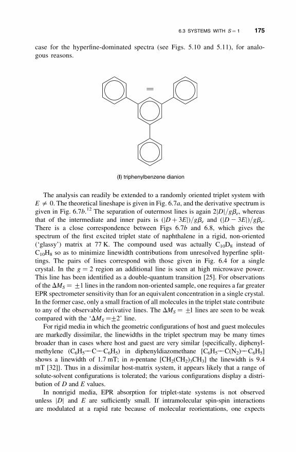
case for the hyperfine-dominated spectra (see Figs. 5.10 and 5.11), for analo-

gous reasons.

The analysis can readily be extended to a randomly oriented triplet system with

E = 0. The theoretical lineshape is given in Fig. 6.7a, and the derivative spectrum is

given in Fig. 6.7b.12 The separation of outermost lines is again 2jDj/gbe, whereas

that of the intermediate and inner pairs is (jDþ 3Ej)/gbe and (jD 2 3Ej)/gbe.

There is a close correspondence between Figs 6.7b and 6.8, which gives the

spectrum of the first excited triplet state of naphthalene in a rigid, non-oriented

(‘glassy’) matrix at 77 K. The compound used was actually C10D8 instead of

C10H8 so as to minimize linewidth contributions from unresolved hyperfine split-

tings. The pairs of lines correspond with those given in Fig. 6.4 for a single

crystal. In the g ¼ 2 region an additional line is seen at high microwave power.

This line has been identified as a double-quantum transition [25]. For observations

of the DMS ¼+1 lines in the random non-oriented sample, one requires a far greater

EPR spectrometer sensitivity than for an equivalent concentration in a single crystal.

In the former case, only a small fraction of all molecules in the triplet state contribute

to any of the observable derivative lines. The DMS ¼+1 lines are seen to be weak

compared with the ‘DMS ¼+2’ line.

For rigid media in which the geometric configurations of host and guest molecules

are markedly dissimilar, the linewidths in the triplet spectrum may be many times

broader than in cases where host and guest are very similar fspecifically, diphenyl-

methylene (C6H522C22C6H5) in diphenyldiazomethane [C6H522C(N2)22C6H5]

shows a linewidth of 1.7 mT; in n-pentane [CH2(CH2)3CH3] the linewidth is 9.4

mT [32]g. Thus in a dissimilar host-matrix system, it appears likely that a range of

solute-solvent configurations is tolerated; the various configurations display a distri-

bution of D and E values.

In nonrigid media, EPR absorption for triplet-state systems is not observed

unless jDj and E are sufficiently small. If intramolecular spin-spin interactions

are modulated at a rapid rate because of molecular reorientations, one expects


a spread in the components of D. Since the trace of D is zero, the contribution of the

term ST � D � S may become negligible. Two limiting cases may be considered:

1. When jDj and jEj are large, the modulations of the spin-spin interaction lead to so

short a spin lifetime that the averaged spectrum has undetectably broad lines.

2. When jDj and jEj are very small, the line-broadening effects in non-rigid

media are also small. In the absence of hyperfine splitting, one sees a single

line, as if the spectrum were due to a system with S ¼ 12.

FIGURE 6.5 (a) Theoretical EPR absorption spectrum for a randomly oriented triplet

system (with E ¼ 0) for a given value of D and n (taking g ¼ ge). A zero linewidth is

assumed. The solid curve B corresponds to the curve of Fig. 4.7a; the solid curve A

represents a reflection of B about the central field B0. The central (small dash) trough is the

sum of A and B. Compare with Fig. 5.10 (j ¼ 10). (b) First-derivative curve computed

from (a) after assuming a non-zero linewidth. Only the field region corresponding to

DMS ¼+1 is shown. The points marked x correspond to the resonant field values when

the magnetic field is oriented along Z (cusp-shaped lines) or perpendicular to Z. [After

E. Wasserman, L. C. Snyder, W. A. Yager, J. Chem. Phys., 41, 1763 (1964).]. Note and

tentatively explain the difference between the idealized first-derivative spectrum shown

here, and the one depicted in Fig. 5.11.


A system that may be an example of case 2 is the set of four ions shown below [struc-

ture II; R could be C(CH3)3]. Here two ketyl radical anions (formed by reaction of

carbonyl compounds and an alkali metal) are bound by two alkali ions to form a

quartet cluster [33].

Such systems have very small D values (0.007–0.015 cm21), in solid CH3DMF at

77 K. At room temperature, in liquid DMF, they show a seven-component compo-

site spectrum (intensity ratios: 1 : 2 : 3 : 4 : 3 : 2 : 1) arising from two equivalent

alkali (23Na, I ¼ 32) nuclei, with each proton-split component looking just as if the

second ketyl unit were not present [34].

6.3.4 Photo-excited Triplet-State Entities

We have now developed the theory necessary to interpret the EPR spectra of triplet

(S ¼ 1) systems and are thus in a position to examine specific examples of the appli-

cation of EPR to these systems.

FIGURE 6.6 Triplet-state EPR spectrum of a rigid solution of the di-anion of

1,3,5-triphenylbenzene in methyltetrahydrofuran at 77 K; n ¼ 9.150 GHz. The line R2

arises from the mono-negative ion (see discussion in Section 6.3.6.2). [After R. E. Jesse,

P. Biloen, R. Prins, J. D. W. van Voorst, G. J. Hoijtink, Mol. Phys., 6, 633 (1963).]


There is a very wide range of possibilities for triplet systems. We begin in this

section with the most important category, namely, the large number of systems

that are diamagnetic (S ¼ 0) in the ground state but have relatively long-lived

FIGURE 6.7 (a) Theoretical EPR absorption spectrum (centered at a field B0) of a

randomly oriented triplet system for given values of D0, E0 and n (and g ¼ ge). A zero

linewidth is assumed. (b) First-derivative curve computed from (a) after assuming a non-

zero linewidth. Only the transitions corresponding to DMS ¼+1 are shown. The points

marked x correspond to resonant-field values at which the magnetic field is oriented along

one of the principal axes of D of the system. [After E. Wasserman, L. C. Snyder, W. A.

Yager, J. Chem. Phys., 41, 1763 (1964).]


excited triplet states generated by steady-state or flash irradiation. Thereafter we

consider thermally excited triplet entities and, finally, ground-state triplet species.

After irradiation with visible or ultraviolet light, many aromatic hydrocarbons in

rigid solutions at low temperature exhibit excited states of unusually long lifetime—

some of the order of minutes, as manifested by the long-lived glow (phosphor-

escence) remaining after turning off the incident light. This behavior is the result

of the existence of a metastable state, which is populated via other excited states.

G. N. Lewis et al. [35] postulated in 1941 that this long-lived state is a spin

triplet state and that direct excitation to, or emission from, this state is spin-forbidden

(to first approximation). Following Lewis’ prediction, magnetic-susceptibility

experiments on excited aromatic molecules in rigid media yielded results in quali-

tative accord with the triplet nature of the state. That is, on irradiation there is an

increase in paramagnetism; this decays on cessation of irradiation, with the same

decay rate constant as that of phosphorescence.

Aromatic hydrocarbons have been the focus of much of the early EPR triplet

work, partly because of their availability and stability, their well-defined p-electron

systems, and their long triplet lifetimes (no heavy atoms). It is relatively easy to

prepare magnetically dilute systems containing small amounts of the molecules of

interest in a diamagnetic optically inert medium. Thus specific photo-excitation of

the molecules from their diamagnetic (singlet) ground states to populate their

(lowest) triplets should allow study by EPR. However, a number of early exper-

iments failed to detect such triplets. One reason for the initial failures is the

marked anisotropy of the EPR line positions, arising from the dipolar interaction

between the two electrons coupled to give S ¼ 1. A second reason is the low sensi-

tivity of the spectrometers at the time (1950–1955) when these first attempts were

made.

FIGURE 6.8 EPR spectrum at 9.08 GHz of photo-excited triplet perdeuteronaphthalene

(C10D8) in a glassy mixture (‘EPA’) of hydrocarbon solvents at 77 K. Lines in the region

of g ¼ 2 arise from free radicals (S ¼ 12) and from double-quantum transitions. [After

W. A. Yager, E. Wasserman, R. M. R. Cramer, J. Chem. Phys., 37, 1148 (1962).]


Once the cause of the earlier failures was recognized, a successful observation of

the lowest excited triplet state of naphthalene was achieved by irradiating single

crystals of durene (1,2,4,5-tetramethylbenzene) containing a small fraction of

naphthalene.13 Since the two molecules are similar in shape, the naphthalene

directly replaces durene in the lattice.

Optical studies indicate that the singlet-triplet splitting in naphthalene is

�20,000 cm21, and hence that J0 is large enough to ensure that the singlet

excited state does not affect the magnetic properties of the system. Note that the

EPR spectrum of a triplet system yields no explicit information about the exchange

parameter(s). An electronic energy diagram, patterned after the one originated by

A. Jablonski in 1933, is shown in Fig. 6.9.

The EPR spectra observed for naphthalene are precisely in accord with the

expectations for a system with S ¼ 1. The positions of EPR lines for the three

principal-axis orientations of the field are given in Figs. 6.4a–c. It was found

[10,37] that D ¼ 0.1003 cm21, E ¼ 20.0137 cm21 (D0 ¼ 107.3 mT and

E0 ¼ 214.7 mT), and g (isotropic) ¼ 2.0030. The principal-axis system for D, as

related to the molecular frame, is shown in Figs. 6.4 and 6.9. The lines in the vicinity

of hn/2gbe were considered in Section 6.3.2. The zero-field splitting parameters

shown above are relatively small. This is consistent with the Pauli exclusion

FIGURE 6.9 The lowest electronic singlet and triplet energy levels of naphthalene,

showing photon absorption, fluorescence and phosphorescence transitions and their mean

lifetimes, as well as radiation-less transitions (wavy lines). The zero-field splittings of the

lowest triplet are indicated at the right.


principle and the coulombic repulsion between the two mobile unpaired electrons,

which causes them to stay apart, decreasing the dipolar interaction energy and

hence jDj.

The line positions as a function of orientation for triplet naphthalene in a

single crystal of durene, for the magnetic field oriented in the xy, xz and yz

planes of the crystal, are shown in Fig. 6.10. The spectra include contributions

from the two types of sites in the unit cell, one of which (site 1) is scanned in

its D principal planes. The reader is urged to interpret the angular-dependence

FIGURE 6.10 Angular dependence of the resonant field (at 9.7 GHz) for triplet

naphthalene in durene, as a function of rotation with B in several planes for the two

symmetry-related molecules (the planes are defined in Fig. 6.4). Hyperfine effects are

ignored. [After C. A. Hutchison Jr., B. W. Mangum, J. Chem. Phys., 34, 908 (1961).]


curves and to extract the zero-field splitting parameters D and E (Problems 6.5

and 6.6).

For the naphthalene triplet state in a durene single crystal, with B along the X or Y

principal axes, a 1 : 4 : 6 : 4 : 1 quintet can be resolved at 77 K [38]. By employing

variously deuterated samples, it was determined that the hyperfine splitting

a ¼ 0.561 mT arises from the 1,4,5,8 protons and a ¼ 0.229 mT from the 2,3,6,7

protons (these values refer to B k Z). These hyperfine splittings are very similar

to those of the naphthalene anion considered in Chapter 3 (Fig. 3.8) (see Section

9.2.2 for further discussion).

Benzene itself has been studied by EPR [39, 40]. The data indicate that the mol-

ecule in its lowest triplet state no longer has D6h symmetry; that is, it is distorted.

There is interconversion among the (three) energy-equivalent configurations, as is

evident from the linewidth behavior. Such transfer of the triplet excitation, here

intramolecular, is a general phenomenon. Thus diffusion of such triplet excitons

[41] can populate triplet states in molecules that were not originally excited by

the ultraviolet irradiation. For example, the EPR signal of phenanthrene can

decrease while that of naphthalene increases after irradiation in biphenyl crystals

doped with both [42].

There exist inorganic systems that display photo-excited metastable triplet states

with optical and magnetic properties closely analogous to those of the aromatic p

systems. We consider the d0 transition ions (e.g., V5þ, Cr6þ, Mn7þ, Mo6þ) in

oxides [43]; for example, the VO432 ion in YVO4 or in Ba3(VO4)2, which, while

diamagnetic in its singlet ground state, exhibits an EPR spectrum when illuminated.

Presumably the optical excitation shifts electrons into the previously empty d shell

with accompanying distortion of the already elongated oxygen tetrahedron

(Fig. 6.11). Studies of EPR at various frequencies (4–23 GHz) and magnetic

fields (including B ¼ 0) have yielded electronic quadrupole (D) splittings (and

mean lifetimes) of the lowest triplet levels (Fig. 6.12) for the vanadate ion dilute

(4%) in YPO4 at 1.2 K [44]. Note the magnitude of the zero-field splittings as

compared to those found for the delocalized p electrons in aromatic systems.

These sensitive measurements, yielding the spin-hamiltonian parameters g, D and

an estimate of A(51V) (Fig. 6.11), were carried out by means of optical detection

of the EPR signals. Here square-wave modulation at 300 Hz of excitation field B1

results in modulation of the phosphorescence detected synchronously at the same

frequency (Chapter 12).

6.3.5 Thermally Accessible Triplet Entities

Sections 6.3.4 and 6.3.6 of this chapter deal with systems in which the triplet state of

interest is a photo-excited state or the ground state. In either case we tacitly assume

that the separation of the triplet state from a nearby singlet state is large enough so

that one need not consider mixing of the two states. An additional interesting case

is that in which the singlet-triplet separation is small enough to make the triplet

state thermally accessible but still not so small as to cause serious mixing of

states. The singlet-triplet separation is approximately jJ0j, where the exchange


FIGURE 6.11 The structure of the YPO4 unit cell, showing a V5þ having replaced a P5þ

ion at the center. For the ground-state singlet, the local symmetry is D2d (as in pure YPO4),

featuring two reflection planes (ac and bc) intersecting at two-fold axis c. It is believed

that distortion removes one such plane in the lowest triplet state. Axes X, Y, Z indicate the

principal axes of D, with axis Z normal to the remaining reflection plane and axis Y

along a V–O direction. Axes Xg, Yg, Zg denote the principal axes of g. [After

W. Barendswaard, R. T. Weber, J. H. van der Waals, J. Chem. Phys., 87, 3731 (1987).]

FIGURE 6.12 The zero-field splitting of the lowest S ¼ 1 state of V5þ in YPO4 at 1.2 K,

also giving the mean lifetime of each level. The sign of D here was taken to be positive; if

it were negative, then the order of the levels would be reversed. The X, Y, Z labeling

follows this book’s convention [W. Barenwaard, R. T. Weber, J. H. van der Waals, J.

Chem. Phys., 87, 3731 (1987)].


interaction between two electrons is given by J0 S1T� S2 (Eqs. 6.3–6.5). When the

triplet lies higher than the singlet (J0 . 0), the relative population of the triplet

state is governed by the Boltzmann factor 3 exp[2J0/kbT ]. In general, for a given

population of a paramagnetic state, the intensity I of EPR absorption is given by

a Curie-law (Eq. 1.16 and Section 10.3.4) dependence, that is, I / 1/T. The inte-

grated intensity I of EPR absorption arising from a thermally excited triplet state

should depend on temperature as

I/ T�1½3þ exp (J0=kbT)��1 (6:40)

Thus a study of the temperature dependence of the EPR intensity (i.e., areaA; see

Section E.1) permits a determination of the value of J0.

A clear-cut example of a thermally accessible triplet state is provided by the Ft

‘point’ defect in MgO [45]. This center is thought to be a neutral trivacancy, that

is, a missing linear (O22Mg22O)22 fragment replaced by two electrons. It gives

no EPR spectrum at very low temperatures, unless ultraviolet (uv)-irradiated. Alter-

natively, a spectrum is generated by warming above 4 K. This indicates that the

triplet state for the two electrons lies above the singlet so that J0 . 0. An analysis

of the temperature dependence yields J0 ¼ 56(7) cm21.14 At arbitrary orientations

of the magnetic field, the EPR spectrum consists of six lines (pairs of DMS ¼+1

transitions, one for each of the three distinct orientations of the

O2222Mg2þ22O22 axes in the cubic crystal). The 300 K line positions as a function

of rotation in the (001) and (110) planes are shown in Fig. 6.13. An analysis of these

data reveals that D0 ¼ 30.7 mT and E ¼ 0, with g ¼ 2.0030(5). From Eqs. 6.41 or

9.18a, the average interelectronic distance is found to be 4.5 A; this compares

well with the relevant oxygen-oxygen distance of 4.2 A in MgO [45].

FIGURE 6.13 Orientation dependence of the X-band EPR lines arising from the Ft center

in MgO at 300 K. [After B. Henderson, Br. J. Appl. Phys., 17, 851 (1966).]


Another interesting example is the observation of a triplet EPR spectrum in

powdered samples of Fremy’s salt, represented here by K4[(SO3)2NO]2 to

emphasize its spin-paired dimeric structure [46]. Here D ¼ þ0.076 cm21 and

E ¼ þ0.0044 cm21. The area of the half-field peak was found to increase expo-

nentially (Eq. 6.40) with temperature (250–350 K), yielding the singlet-triplet

gap energy J0 ¼ 2180 cm21. Since no hyperfine (14N) splitting is observed,

this spectrum has been assigned to a triplet exciton, which is an excited state

that migrates rapidly through the crystal lattice.

6.3.6 Ground-State Triplet Entities

A triplet species need be no larger than an atom if it has an appropriate set of degen-

erate orbitals. The list of ground-state triplet atoms includes C, O, Si, S, Ti and Ni.

The two most prominent ground-state triplet diatomic molecules are O2 and S2

(Chapter 7).

6.3.6.1 Carbenes and Nitrenes The H22C22H fragment (methylene or

‘carbene’) is one of the simplest molecular systems, and the triplet nature of its

ground state has been established spectroscopically. The EPR spectrum of

methylene has been reported (Table 6.1) for both CH2 and CD2. For the former,

D ¼ 0.69 cm21 and E ¼ 0.003 cm21; for the latter, D ¼ 0.75 cm21 and

E ¼ 0.011 cm21. The difference presumably arises from the effect of zero-point

vibration. Many substituted methylenes have also been studied (Table 6.1). The

non-zero value of E for some of these molecules indicates that for them there is

TABLE 6.1 Zero-Field Splitting Parameters for Triplet Ground-State Molecules

Molecule jDj (cm21) jEj (cm21) Reference

H22C22H 0.69 0.003 a

D22C22D 0.75 0.011 a

H22C22C;;N 0.8629 0 b

H22C22CF3 0.712 0.021 c

H22C22C6H5 0.5150 0.0251 d

H22C22C;;C22H 0.6256 0 b

H22C22C;;C22CH3 0.6263 0 b

H22C22C;;C22C6H5 0.5413 0.0035 b

C6H522C22C6H5 0.4055 0.0194 d

N;;C22C22C;;N 1.002 ,0.002 e

N22C;;N 1.52 ,0.002 e

a R. A. Bernheim, H. W. Bernard, P. S. Wang, L. S. Wood, P. S. Skell, J. Chem. Phys., 53, 1280 (1970);

54, 3223 (1971); R. A. Bernheim, R. J. Kempf, E. F. Reichenbecher, J. Magn. Reson., 3, 5 (1970);

E. Wasserman, V. J. Kuck, R. S. Hutton, E. D. Anderson, W. A. Yager, J. Chem. Phys., 54, 4120 (1971).b R. A. Bernheim, R. J. Kempf, J. V. Gramas, P. S. Skell, J. Chem.Phys., 43, 196 (1965).c E. Wasserman, L. Barash, W. A. Yager, J. Am. Chem. Soc., 87, 4974 (1965).d E. Wasserman, A. M. Trozzolo, W. A. Yager, R. W. Murray, J. Chem. Phys., 40, 2408 (1964).e E. Wasserman, L. Barash, W. A. Yager, J. Am. Chem. Soc., 87, 2075 (1965).


no axis of symmetry of order 3 or greater; this indicates that the molecules are non-

linear. For such systems, the maximum number of peaks (six DMS ¼+1 transitions)

is expected in the glass-phase EPR spectrum, just as for naphthalene in the excited

triplet state (Figs. 6.7 and 6.8). When the system is nearly uniaxial, the parameter E

may be so small that one may only be able to set an upper limit for its value. An

increase in the extent of the conjugated system attached to the methylene carbon

atom may lead to a decrease in the parameter D as is evident from Table 6.1.

Figure 6.14 shows the energy-level diagrams for the fluorenylidene molecule

(III) [47]. The molecule is generated in its ground triplet state by irradiation of

diazofluorene at 77 K. It is thus to be regarded as a derivative of methylene. If

the zero-field splitting D is large compared with hn for a microwave quantum,

only certain of the lines allowed by the selection rules are observed. When B is par-

allel to axis X or Y, only one transition is observed for n � 9.7 GHz. Since the ordi-

nate in Fig. 6.14 is expressed in gigahertz, the frequency required to cause a

transition between adjacent levels is immediately apparent from it. For B k Z,

three transitions are expected and are observed. Two of these are between the

levels designated by j0l and j–1l. Note (Fig. 6.14c) that the ‘DMS ¼+2’ transition

occurs at an intermediate value of the magnetic field. The parameters measured,

jDj ¼ 0.4078 and jEj ¼ 0.0283 cm21, are appreciably larger than those of naphtha-

lene, as expected (Section 6.3.4). The reader should compare the resulting tran-

sitions allowed at X band (Figs. 6.4 and 6.14).

FIGURE 6.14 Energy levels of the fluorenylidene molecule (III) in its triplet ground state

as a function of applied magnetic field (measured in proton NMR fluxmeter frequency units).

The EPR transitions indicated are at �9.7 GHz. (a) B k X; (b) B k Y; (c) B k Z. Here

jDj ¼ 0.4078 and jEj ¼ 0.0283 cm21. [After C. A. Hutchison Jr., G. A. Pearson, J. Chem.

Phys., 47, 520 (1967).]


Another organic triplet species of considerable experimental and theoretical

interest is trimethylenemethane (IV), which can be represented as

This free radical, TMM,15 can be prepared by g irradiation of methylenecyclopropane.

EPR studies [49] reveal that it is a triplet ground-state species, rather than a biradical;

that is, jJ0j is relatively large compared to jDj, and parameter J0 is negative (see

Fig. 6.2). The radical has four p electrons, and is close to uniaxial (planar with sym-

metry D3h) as inferred from the parameters D ¼ 0.0248 cm21 and E , 0.003 cm21, at

77 K. The temperature dependence of these parameters, and of the proton hyperfine

matrix (six equivalent protons, principal values Ai/h of 214, 238 and 226 MHz)

suggests that anisotropic rotational effects occur. Because the proton nuclear

Zeeman term is not small compared to the hyperfine values in this anisotropic

system, all four hyperfine transitions per proton are observed (Section 5.3.2.1). The

relative sign of D and A, obtainable from the EPR data, discloses that D is positive.

From Eq. 6.15a (D diagonal) and Eq. 6.25a, it is easily shown that

D ¼3m0

16pg2be

2hr�3ih1� 3 cos2 u i (6:41)

Here angle u is the angle between the inter-electron (spin) vector r and the principal

axis Z of D. It is evident that the sign of D is determined solely by k1 2 3 cos2 ul. If

the dipoles were fixed at two points (in which case r/r ¼ Z and 12

DZ ¼ 2DY ¼ –DX),

Eq. 6.41 would yield D ¼ 2(3 m0/8p)g2be2kr –3l, that is, D would be negative. For a

triplet-state atom not in an electric field, the spherical symmetry dictates that D ¼ 0. In

non-spherical systems, D can be negative or positive. The latter sign occurs in binuc-

lear triplet species when the internuclear axis is perpendicular to Z, as dictated by the

unpaired-electron distribution. In trimethylenemethane (IV), the two unpaired elec-

trons can be considered as being equally distributed at three points (carbons) in a

plane normal to the symmetry axis, so that D . 0.

6.3.6.2 Dianions of Symmetric Aromatic Hydrocarbons A molecule

may have a ground triplet state in its neutral, cationic or anionic form. Here there

is one unpaired electron in each of a pair of degenerate orbitals. Thus, as is

shown in Fig. 6.1d, the lowest-energy state (ground state) is that corresponding to

single occupation with parallel spins of the highest two occupied levels.

Degenerate orbital energy levels are found in molecules with an n-fold (n � 3)

axis of symmetry. Molecules of this type do not necessarily have a triplet ground


state. The situation depends on the sign of the electron-exchange integral (Eq. 6.5).

If J0 is positive, then the singlet state lies lower. This is the case, for instance, in the

coronene di-anion with alkali counterions (V) [49,50].

Occurrence of one electron in each of two degenerate orbitals of symmetrically

substituted benzenes may be achieved if the di-anion can be formed. Triplet

ground states have been demonstrated for symmetric molecules such as the

1,3,5-triphenylbenzene (I) and triphenylene di-anions (VI).

These ions possess degenerate antibonding orbitals, analogous to those shown in

Fig. 6.15 for the hypothetical benzene di-anion (note Table 9A.2). For the triphenyl-

benzene di-anion (ground triplet state, Fig. 6.6) D is less (D ¼ 0.042 cm21) than that

of the neutral excited triplet-state molecule (D ¼ 0.111 cm21) [51]. The orbital

occupation is very different for these two cases; calculations show that in the

excited triplet molecule, there is a greater interaction (leading to a larger D value)

between two electrons in the ‘paired’ bonding and antibonding orbitals than

between two electrons in the antibonding orbitals of the ground-state di-anion.

6.3.6.3 Inorganic Triplet Species Other than O2 and S2 (considered in

Chapter 7) and some transition-ion complexes, there are not many stable inorganic

molecules that exist in a triplet ground state. Some unstable species can be trapped in

low-temperature matrices. Excellent examples are the isoelectronic molecules CCO


and CNN, prepared by reaction of C atoms with CO or N2 with subsequent trapping

in a frozen rare-gas matrix at 4 K [52]. Both of these molecules have large values of

D (D ¼ 0.7392 cm21 for CCO and D ¼ 1.1590 cm21 for CNN in solid neon) such

that D . hn at X band. Thus only one transition is seen in each case. The 13C and14N hyperfine parameters are also reported. The fact that E ¼ 0 indicates that these

molecules are linear.

Another quite different example of a ground-state triplet is the quasi-tetrahedral

[AlO4]þ ‘point’ defect in a quartz single crystal [53]. This center is believed to

contain two electron holes forming a triplet spin system in which the two unpaired

electrons are �0.265 nm apart on adjacent (and symmetry-related) oxygens in the

AlO4 entity. For this center at �35 K, D0 ¼ 269.8 mT and E0 ¼ 6.3 mT. These

values are in very good agreement with those calculated on the basis of a model

placing an unpaired-electron population of 0.76 in two oxygen 2p orbitals perpen-

dicular to the Al22O22Si plane. As expected [3], the hyperfine matrix from the

central 27Al ion is accurately approximated by A ¼ (A1þA2)/2, where matrices

A i (i ¼ 1, 2) stem from the corresponding radicals (S ¼ 12) centered on the two

oxygens. Similarly, g ¼ (g1þ g2)/2. The hyperfine splittings arising from the low-

abundance isotope 29Si, that is, from outer silicon atoms bonded to the oxygens, are

half as large as the corresponding ones from the S ¼ 12

species.

Various transition ions provide examples of S ¼ 1 systems, for example, V3þ and

Ni2þ in the 3d series (Chapter 8). The latter ion, dilute in K2MgF4 where it is in a

Mg2þ site surrounded by a slightly distorted octahedron of F2 ions, yielded

D ¼ 20.425 cm21 and E ¼ –0.065 cm21 (with isotropic g ¼ 2.275) at 1.6 K [54].

6.4 INTERACTING RADICAL PAIRS

The earliest EPR work in this specialty area is that done by Bleaney and Bowers [55]

and also by Kumagai et al. [56], on cupric acetate monohydrate, in which Cu2þ 3d1

ions, each influenced by the local electric field, also interact pairwise and reveal an

FIGURE 6.15 Triplet p-electron configuration of the hypothetical benzene di-anion.

6.4 INTERACTING RADICAL PAIRS 189

effective electron spin of S ¼ 1 (g? ¼ 2.08 and gjj ¼ 2.42) at 90 K. The electronic

quadrupolar parameters are D/hc ¼ 0.34 cm21 and E/hc ¼ 0.01 cm21. There are

5 � 5 orbital states, with a singlet lowest, each such state with spin degeneracy of

2 � 2 (neglecting nuclear Cu spins; these do, however, give rise to observed hyper-

fine structure). The resulting ground state is a singlet (diamagnetic), while the lowest

excited state is a triplet. The latter becomes appreciably populated even at quite low

temperatures (.50 K) and gives rise to the observed EPR spectrum. The splitting

J0/hc (aboutþ300 cm21; see Eq. 6.4) between the singlet and triplet states, as deter-

mined from the temperature dependence of the EPR intensity, is caused primarily by

the electronic exchange interaction. Thus, here, jJ0j gbeB. The anisotropy of the g

value indicates presence of appreciable spin-orbit interaction.

In the case of strongly coupled spin ¼ 12

identical pairs with nuclear spins, such as

described above, the hyperfine coupling parameters have magnitudes half as large as

the corresponding values for the single entities.

The case of weakly coupled radical pairs (jJ0j gbeB) has been successfully

treated by Itoh et al. [57]. Here the singlet and triplet are mixed by the Zeeman

and hyperfine interactions, and J0 can be evaluated from the EPR line positions.

This has been done for pairs of RR0C55NO free radicals created by irradiation of

single crystals of glyoximes [57]; for R ¼ R0 ¼ CH3, J0/hc ¼ þ0.200 cm21.

Obviously, far more detail on the spin-pair systems will be sought. Thus, the

exact distances between the pair units, in both the singlet and triplet states, will

be welcomed, as will the orientations of these axes within the crystals. Advanced

techniques, such as ELDOR in ESE studies (see Chapters 11 and 12), are expected

to be helpful in such efforts [58].

6.5 BIRADICALS

As indicated above, a biradical is a molecule containing two unpaired electrons

that, on the average, are so far apart that interactions between them are sufficiently

weak and energy classification into a singlet and a triplet manifold is not useful.2

More generally, this category includes radical pairs, in which the spins are

located on close but separate species.

The border region between triplet-state species and biradicals is, of course,

nebulous, as it is set by the magnitudes of D and E compared to that of the

singlet-triplet energy separation. We note that as D and E! 0, the half-field

transition remains pretty well in place (see Eq. 6.36b), but declines rapidly in

intensity. For triplet states, jD/hcj typically is in the range 0.1–2.5 cm21

(Section 6.3), but it is this magnitude compared to that of exchange energy par-

ameter J0 which is the crucial factor. Thus TMM previously discussed has a

triplet ground state with D/hc � þ0.025 cm21, while J0/hc is estimated to

be 25000 cm21 [59].

Consider a biradical composed of two identical molecular fragments, each

containing one unpaired electron as well as one magnetic nucleus giving rise to

hyperfine splitting. We consider the isotropic case. The spin hamiltonian appropriate


to this system is [60,61]16

H ¼ gbeB(S1z þ S2z)þ A0(S1T� I1 þ S2

T� I2)þ J0S1T� S2 (6:42)

Here we consider the biradical to exist in liquid solution so that the anisotropies

arising from g, D and T are averaged to zero. We neglect the effect of the nuclear

Zeeman terms, the cross-hyperfine interactions, and the nucleus-nucleus spin coup-

lings. If jA0j gbeB, then the hyperfine terms may be taken to first order only, and

Eq. 6.42 can be approximated as

H ¼ gbeB(S1z þ S2z)þ A0(S1zI1z þ S2zI2z)þ J0S1T� S2 (6:43)

where B k z.

First, consider the limiting case where jJ0j jA0j. The zero-order spin

hamiltonian is then

H0 ¼ gbeB(S1z þ S2z)þ J0S1T� S2 (6:44a)

which can be expanded (Section C.1) to yield

H0 ¼ gbeB(S1z þ S2z)þ J0 S1zS2z þ12

(S1þS2� þ S1�S2þ)h i

(6:44b)

The appropriate eigenfunctions are

j1,þ1i ; jþ 12

,þ 12i (6:45a)

j1, 0i ;1ffiffiffi

2p jþ 1

2, �1

2i þ j�1

2, þ 1

2i

� �

(6:45b)

j1,�1i ; j�12

,�12i (6:45c)

j0, 0i ;1ffiffiffi

2p jþ1

2, �1

2i � j� 1

2, þ1

2i

� �

(6:45d)

The quantum numbers in the right-hand set of kets (uncoupled representation)

refer to the eigenvalues of S1z and S2z, whereas those on the left (coupled represen-

tation) refer to the quantum numbers S and MS arising from S2

and Sz, where

Sz ¼ S1z þ S2z.

6.5 BIRADICALS 191

The energies to first order (in A0 and J0; note and compare Figs. 6.2 and 6.15, in

which A0 is neglected) are

U1, þ1(1) ¼ þgbeBþ J0=4þ A0

tMI=2 (6:46a)

U1,0(1) ¼ þJ0=4 (6:46b)

U 1, �1(1) ¼ �gbeBþ J0=4� A0

tMI=2 (6:46c)

U0,0(1) ¼ �3J0=4 (6:46d)

Here tMI ¼ MI1þMI2

. The only allowed EPR transitions are j1, +1l$ j1,0l,which are degenerate at a transition energy of gbeBþ A0MI/2 and are independent

of J0. In the case of I1 ¼ I2 ¼ 1, the first-order spectrum would consist of five lines

separated by ja0j/2 (where a0 ¼ A0/gebe) with intensity ratios 1–2–3–2–1, sincetMI ¼ �2, �1, 0, þ1, þ2. An example of this case is the EPR spectrum of the bir-

adical tetramethyl-2,2,5,5-pyrrolidoneazine-3 dioxyl1,10 (VII), shown in Fig. 6.16a,

where the line separation is only 0.740 mT so that a0(14N) ¼ 1.480 mT [62].

FIGURE 6.16 (a) X-band EPR spectrum of biradical VII showing interaction of both

unpaired electrons with nitroxide 14N nuclei. The spacing is ja0j/2, where ja0j ¼ 1.480 mT

is the spacing for the corresponding monoradical (one NO group replaced by NH). [After

R. M. Dupeyre, H. Lemaire, A. Rassat, J. Am. Chem. Soc., 87, 3771 (1965).] (b) X-band

EPR spectrum of the biradical VIII, in which the nitroxide groups are isolated from each

other. The hyperfine splitting (1.56 mT) is just the same as that of the corresponding

monoradical. This is an illustration of the case jJ0j jA0j. [After R. Briere, R. M. Dupeyre,

H. Lemaire, C. Morat, A. Rassat, P. Rey, Bull. Soc. Chim. France, No. 11, 3290 (1965).]


Now consider the second limiting case, of jJ0j jA0j. The zero-order spin

hamiltonian is

H0 ¼ gbeB(S1z þ S2z)þ A0½S1zI1z þ S2zI2z) (6:47)

This operator is separable into two parts

H0(1) ¼ gbeBS1z þ A0S1zI1z (6:48a)

H0(2) ¼ gbeBS2z þ A0S2zI2z (6:48b)

The eigenfunctions of H0(1) are

jþ12

, MI(1)i and j� 12

, MI(1)i

with eigenvalues

Uþ1=2(0) ¼ þgbeB=2þ A0MI(1)=2 (6:49a)

U�1=2(0) ¼ �gbeB=2� A0MI(1)=2 (6:49b)

One obtains analogous results for H0(2). Thus this case may be considered as

two non-interacting systems with S ¼ 12. When I ¼ 1, the first-order EPR spectrum

consists of three lines separated by ja0j. An example of this case is shown

in Fig. 6.16b, where the biradical is di(tetramethyl-2,2,6,6-piperidinyl-4

6.5 BIRADICALS 193

oxyl-1)terephthalate (VIII).

The intermediate case of jJ0j � jA0j gives rise to a complex group of lines.

The intensity and position of these lines are a strong function of jJ0/A0j [63–65].

Thus J0 can be extracted from the solution EPR spectrum.

The general case, when one encounters anisotropic parameters and where field B

is of arbitrary magnitude, can be dealt with using the spin hamiltonian

H ¼ beBT� g1� S1 þ beBT� g2� S2 þ12

(S1T� J� S2 þ S2

T� JT� S1)

þ nuclear terms as needed(6:50)

The EPR line positions and relative intensities are obtainable from Eq. 6.50 by

numerical (computer) solution. An example of the energy levels for such a case is

depicted in Fig. 6.17.

FIGURE 6.17 The energy levels U(MS1, MS2

) as a function of applied magnetic field B for

a biradical system not containing any nuclear spin. The primary EPR transitions

(DMSi¼+1), involving the two MSi

¼ 0 levels, are shown. No nuclear spins occur here.

The spin-hamiltonian parameters (Eq. 6.50) used to generate the figure are taken from

J. Isoya, W. C. Tennant, Y. Uchida, J. A. Weil, J. Magn. Reson., 49, 489 (1982).


Note that the three matrices in Eq. 6.50 are attainable by computer analysis of

single-crystal EPR rotational data, where J includes the isotropic exchange par-

ameter J0 as well as the spin-spin dipolar interaction and anisotropic exchange.

6.6 SYSTEMS WITH S > 1

A few organic high-spin radicals are known. For instance, the assembly of the three

diphenylhydrazyl groups (Section E.1.2) mounted meta to each other on a central

1,3,5-tricyanobenzene yields a stable triradical (S ¼ 32), exhibiting DMS ¼+1, +2

and +3 transitions [66]. Perhaps the highest spin multiplicity known for organic mol-

ecules at this time is an undecet ground state, arising from the five sets of unpaired

electrons formally located at five methylene carbons held between phenyl groups,

in the meta-linked molecule C6H522C22(C6H422C22C6H422C22)2C6H5 (having

S ¼ 5) prepared and studied by EPR [67]. More accurately, five of the unpaired

electrons are delocalized in a p orbital; the other five occur in s non-bonding orbitals.

Monatomic high-spin species can be created (e.g., by irradiation procedures), and

have been studied since the mid-1950s or 50. A good example is the nitrogen atom,

whose electronic ground state (S ¼ 32) is 4S3/2 (see Section B.7). Such atoms can be

trapped and stabilized in solid matrices (e.g., in molecular nitrogen at low tempera-

tures [68], in azides [69], and in fullerene cages [70]), in liquids (e.g., superfluid

helium [71]), and in gas phase (see Section 7.2). For N0, typical parameters are

g ¼ 2.002, D ¼ 0.010 cm21, E ¼ 20.002 cm21 (the latter two measured, of

course, in solids) and a0(14N) ¼ 0.5 mT. Because of the high mobility of the

atom, D and E are quite temperature-sensitive.

Numerous other inorganic systems offer high-spin (S . 1) species. These include

clusters of adjacent unpaired electrons (i.e., of F centers) in alkali halides. For

instance, three F centers forming an equilateral triangle in the (1,1,1) plane of a

KCl crystal constitute an S ¼ 32

center, which has been studied by both EPR and

ENDOR [72].

Clusters of transition atoms also lead to high-spin systems. Thus Mn2 and Mn5,

in rare-gas matrices, are amenable to study by EPR [73]. For Mn2, since the

exchange parameter J0 is negative (J00 ¼ 211.0 T, i.e., antiferromagnetic coup-

ling), this molecule features a diamagnetic ground state. However, higher spin

states (S ¼ 1,2,3) can be thermally populated and yield EPR spectra with charac-

teristic 55Mn (I ¼ 52

) hyperfine structure. The pentamer cluster Mn5 has a total spin

S ¼ 252

.

More recently, single-molecule magnets (SMMs) have been studied at very high

frequencies (40–200 GHz). EPR spectroscopy has yielded information about the

energy levels and power saturation behavior of molecular nanomagnet crystals,

including ferric complexes (abbreviated ‘Fe8’) and manganese complexes (abbre-

viated ‘Mn12’ [74,75]). Both have effective spin: S0 ¼ 10.

Clearly, the primary domain of high-spin species is that of transition ions

(Chapter 8), which have been a fruitful source of EPR progress since the beginnings

of this field.

6.6 SYSTEMS WITH S .1 195

6.7 HIGH-SPIN AND HIGH-FIELD ENERGY TERMS

For magnetic species with S . 1, additional terms (e.g., Eqs. 8.17) should be

added to the spin hamiltonian (Eq. 6.18), at least in principle. These usually

make only relatively small contributions to the total energy of the system but

show up as corrections to the EPR line positions and intensities. They are not as

simple as the terms in Eq. 6.18, since tensorial entities greater than rank 2 (not

expressible as matrices) enter, and each term brings in a multitude of parameters

to be obtained from the EPR data. Table 6.2 indicates what types of terms are in

principle allowed. This table is a listing of what terms can be present for each

value of S, ignoring nuclear-spin terms. The symbol S implies the possible

presence of all three operators Sx, Sy and Sz. Operator S2 indicates the term

ST � D � S discussed in this chapter. Similarly, the symbol B here implies the

possible presence of Bx, By and Bz. Integers n, n0 and n00 are positive odd

integers; thus n ¼ 1 indicates the usual electron Zeeman term, and all other inte-

gers n (and all n0, n00) are usually safely ignored (except in highly accurate

measurements).

Column 2 in Table 6.2 includes the high-field situation (for any S ) in which one

considers that all spin-hamiltonian parameters are field-dependent. For instance, the

Zeeman splitting factor can be written as the series

g ¼ g(0) þ g(2)B2 þ g(4)B4 þ � � � (6:51)

Here g(0) is the usual g factor, and the g(2) term describes an energy term having the

form of components of B3S (e.g., Bx3Sy), which may become appreciable in the

analysis of ultrahigh-field EPR spectra.

TABLE 6.2 Possible Electron-Spin Magnetic-Field Terms

in the Spin Hamiltoniana

S H Terms

12

SBn

1 SBn S2

32

SBn S2 S3Bn0

2 SBn S2 S3Bn0 S4

52

SBn S2 S3Bn0 S4 S5Bn00

.

.

.

a The meaning of the symbols S and B in this table are defined in the text

(Sections 6.6 and 8.3). Exponents n, n0 and n00 generally are positive

integers.


In accordance with Table 6.2, a term of the form BS3 can occur for S . 1

[76–78]. With smaller S, for example, S ¼ 12, S3 can always be written as a linear

combination of terms at most linear in S. Terms of this type can arise

from the product in perturbation theory of the normal Zeeman term gebeBT � S

and the square (lLT� S)2 of the spin-orbit term [79]. For octahedral or tetrahedral

symmetries, the additional terms have the form

g0be½BXSX3 þ BY SY

3 þ BZSZ3 � BT� S(3 S

T� S� 1)=5�

Here the operator form of the last term is a notational formality: ST� S ¼ S(Sþ 1)

and 1 ¼ 1. With lower symmetry, the number of BS3-type terms increases, and

there is proliferation of the parameters describing the effect [78]. Conversely, if

description of an experimental spectrum requires such a term, this confirms the

identification of an S . 32

state. If there is a nucleus contributing splitting, an

additional term of the form S3 I may also be required.

The derivation and treatment of the terms in Table 6.2 are outside the scope of

this book. The reader is referred to a variety of sources for this type of treatment

[78, 80–86]. Note the special diagrammatic methods in Ref. 83.

6.8 THE SPIN HAMILTONIAN: A SUMMING UP

In the previous chapters, we focused on quantitative description of the Zeeman split-

tings (g), nuclear hyperfine and quadrupolar effects (A, P), and the electronic quad-

rupolar and high-spin interactions (D, . . .). In general, these parameters can all occur

simultaneously for any given paramagnetic species. Thus, to describe the EPR

spectra (as well as other spectra, e.g., ENDOR), it is necessary to add together all

possible terms17 into a single spin hamiltonian

H¼ gbeBT� Sþ ST�D� SþX

N

i¼1

(ST�Ai� Ii�bnBT�gni� Iiþ IiT�Pi � Iiþ�� )

(6:52)

encountered for any electron spin (composite or not) and N nuclear spins, all

contributing to the spectrum. Which terms must be included to analyze any

given spectrum is a matter of judgment and experience, added to an understand-

ing of the chemical system being investigated. The correct spin hamiltonian

yields the observed positions and relative intensities of the lines, in the

absence of dynamic effects (Chapter 10). However, exact energies and transition

probabilities obtained by parameter fitting (i.e., repeated diagonalization of H

by computer) are always possible, generally with some loss of intuitive under-

standing. One important mental exercise regarding Eq. 6.52 is to note which

terms depend on B and which do not (zero-field terms), since the choice of

6.8 THE SPIN HAMILTONIAN: A SUMMING UP 197

spectral region (B region) selected to work in is significantly affected by this

aspect.

Let us now discuss the signs associated with any parameter matrix Y. The relative

signs of the matrix elements Yij are all obtainable from the positions of the EPR lines.

However, determination of the absolute sign (i.e., which of +Y is correct) may not

always be possible. If several matrices (e.g., g, D, A, P) are important in the spin

hamiltonian, the relative signs of some pairs may be available from the data, even

though the absolute sign of the set is not. In some cases the relative signs of A

and P for a particular nucleus may be fixed by the data, but not necessarily with

respect to A and P of some other nucleus also exhibiting line splittings. Special

auxiliary measurements may be needed (see Note 4 in Chapter 4 regarding matrix

g and Section 6.3.1 for matrix D) to arrive at the most complete sign information.

In summary, determination of the signs of spin-hamiltonian parameters is a non-

trivial task.

An approach to visualization of the energy terms arising from a given H is to

resort to a perturbation treatment. We now undertake a brief discussion of the

results of this approximation technique.

Consider a simplified version of Eq. 6.52, namely

H ¼ gbeBT� Sþ ST�D � Sþ ST�A� I (6:53)

of Eq. 6.52, incorporating the now familiar terms from Chapters 4 and 5. For suffi-

ciently large field B, the first term dominates (if MS = 0) and the other two can be

treated as perturbations [87, 88]. The resulting single-nucleus second-order energy

expressions, valid for any S and I, and for any coordinate system are

U(MS;MI) ¼ gbeBMS þ12

d1 3MS2 � S(Sþ 1)

�

þ

1

2 gbeB(d2 � d1

2) 8MS2 þ 1� 4S(Sþ 1)

�

MSþ

1

8 gbeBtr(D)2 � 2d2 þ d1

2 � 2d�1 det(D)�

2S(Sþ 1)� 2MS2 � 1

�

MSþ

KMSMI þ1

2 gbeB

n

12

tr(A�AT)� k12

�

MS I(I þ 1)�M 2I

�

� :

det(A)

KS(Sþ 1)�MS

2�

MI þ (k12 � K2)MS M 2

I þ

2(e� d1)K 3MS2 � S(Sþ 1)

�

MI

o

(6:54)


Here

g2 ¼ nT� g � gT�n (6:55a)

dn ¼ nT� g �Dn� gT� n=g2 (6:55b)

K2 ¼ nT� g �A�AT� gT�n=g2 (6:55c)

k1 ¼ nT� g �A�AT�A �AT� gT� n=g2K2 (6:55d)

e ¼ nT� g � 12

(D �A �AT þ AT�A �D) � gT� n=g2K2 (6:55e)

and, as before, n ¼ B/B. Equation 6.55a is the same as Eq. 4.12. We note the pre-

sence in Eq. 6.54 of terms in B21; higher-order perturbation treatment would give

further terms, in B – 2, and so on. The terms in d– 1, d1, d2, K, k1 and e demonstrate

the intermingling of the three spin-hamiltonian terms in Eq. 6.53 in arriving at the

energy expression.

Obviously, from the energy expression 6.54, it is now possible to derive anisotro-

pic spectroscopic frequencies [U(MS0,MI

0) – U(MS,MI)]/h to be compared with

experiment (e.g., see Eqs. 6.34). Similar perturbation techniques are available to

derive transition moments, that is, relative intensities [89].

When more than one spin-bearing nucleus is present, there are naturally hyperfine

terms in Eq. 6.53, for each nucleus, with resulting energy terms in Eq. 6.54 [90].

Even though no terms coupling the nuclear spins directly have been added to the

spin hamiltonian (since such interaction energies are negligibly small), pair-wise

cross-terms that depend on MIiand MIj

will nevertheless occur in Eq. 6.54; these

arise from electron-mediated dipolar interactions. As usual, for each nucleus with

I . 12, quadrupole terms (Eq. 5.50) should be added to Eq. 6.53.

As more and more terms are included (e.g., nuclear-quadrupole energies [90]),

the perturbation energy expressions become increasingly complicated and unwieldy.

Clearly, also, the limited applicability of perturbation theory must be kept in mind.

Nevertheless, Eq. 6.54 (or its variants) have proved very useful and yield important

insights.

Finally, it should be pointed out that the general spin hamiltonian (Eq. 6.52),

including all high-spin terms, can be formulated in a far more compact and math-

ematically elegant form, involving spherical-tensor operators [76,80–85,90]. Thus

all the matrices (g, D, A i, P i) can readily be expressed in terms of the relevant expan-

sion coefficients. The higher-order terms (not formulatable in terms of 3 � 3

matrices) are also easily presented. However, all too many different versions and

notations regarding this operator structure appear in the literature.

6.9 MODELING THE SPIN-HAMILTONIAN PARAMETERS

Since the mid-1990s with advent of ever more capable rapid computing systems, the

accurate modeling of all the magnetic resonance parameters (e.g., g, A, P, D, . . .) has

become feasible, and thus there is now quite a burgeoning literature on this topic.

6.9 MODELING THE SPIN-HAMILTONIAN PARAMETERS 199

We can cite the text Calculation of NMR and EPR Parameters [91], which presents a

nice overview. As specific examples, we can indicate the density functional theor-

etical (DFT) calculation of g matrices, from first principles, say, for paramagnetic

diatomic molecules and defect centers in crystalline quartz [92]. For the latter

medium, the detailed structural configuration and the 17O, 27Al and 29Si hyperfine

parameter matrices for the famed center [AlO4]0 have been very successfully calcu-

lated [93,94]. Years of such work by Ziegler and his group [95–97], and others, has

borne much fruit; for instance, their inclusion of spin orbit coupling has indicated the

general occurrence not only of spin singlet-triplet mixing but also the resulting

appearance of non-zero spin density on the atoms even of diamagnetic molecules.

Simultaneous inclusion of higher-order spin-orbit and spin-polarization effects in

a relativistic calculation of electronic g matrics were reported in 2005 [98].

REFERENCES

1. P. W. Atkins, R. S. Friedman, Molecular Quantum Mechanics, 4th ed., Oxford Univer-

sity Press, Oxford, U.K., 2005, pp. 225–227.

2. A. Bencini, D. Gatteschi, EPR of Exchange Coupled Systems, Springer, Berlin,

Germany, 1990.

3. J. Owen, E. A. Harris, “Pair Spectra, Exchange Interactions”, in Electron Paramagnetic

Resonance of Transition Ions, S. Geschwind, Ed., Plenum Press, New York, NY,

U.S.A.,1972, Chapter 6.

4. A. Abragam, B. Bleaney, Electron Paramagnetic Resonance of Transition Ions, Claren-

don, Oxford, U.K., 1970, Section 9.3.

5. G. E. Pake, T. L. Estle, The Principles of Electron Paramagnetic Resonance, 2nd ed.,

Benjamin, Reading, MA, U.S.A., 1973, pp. 157–161.

6. N. W. Ashcroft, N. D. Mermin, Solid State Physics, Saunders, Philadelphia, PA, U.S.A.,

1976, p. 680.

7. J. E. Harriman, Theoretical Foundations of Electron Spin Resonance, Academic Press,

New York, NY, U.S.A., 1978, p. 191.

8. R. E. Coffman, A. Pezeshk, J. Magn. Reson., 70, 21 (1986).

9. P. L. Hall, B. R. Angel, J. P. E. Jones, J. Magn. Reson., 15, 64 (1974).

10. A. W. Hornig, J. S. Hyde, Mol. Phys., 6, 33 (1963).

11. H. Schuch, F. Seiff, R. Furrer, K. Mobius, K. P. Dinse, Z. Naturforsch., 29a, 1543

(1974).

12. Y. Yamaguchi, N. Sakamoto, J. Phys. Soc. Jpn., 27, 1444 (1969).

13. H. F. Hameka, L. J. Oosterhoff, Mol. Phys., 1, 358 (1958).

14. P. Kottis, R. Lefebvre, J. Chem. Phys., 39, 393 (1963), Eq. 6.

15. O. Claesson, A. Lund, J. Magn. Reson., 41, 106 (1980), Eq. 2.

16. T. Castner Jr., G. S. Newell, W. C. Holton, C. P. Slichter, J. Chem. Phys., 32(3), 668

(1960).

17. J. S. Griffith, Mol. Phys., 8, 213 (1964).

18. R. Aasa, T. Vanngard, Ark. Kemi, 24(18), 331 (1965).


19. D. G. McGavin, W. C. Tennant, J. Magn. Reson., 62, 357 (1985).

20. R. Berger, J. Kliava, E. Yahiaoui, J.-C. Bissey, P. K. Zinsou, P. Beziade, J. Non-Cryst.

Solids, 189, 151 (1995).

21. M. S. de Groot, J. H. van der Waals, Mol. Phys., 3, 190 (1960).

22. J. H. van der Waals, M. S. de Groot, Mol. Phys., 2, 333 (1959).

23. P. Kottis, R. Lefebvre, J. Chem. Phys., 41, 379 (1964).

24. I. M. Brown, P. J. Phillips, D. Parikh, Chem. Phys. Lett., 132(3), 273 (1986).

25. W. A. Yager, E. Wasserman, R. M. R. Cramer, J. Chem. Phys., 37, 1148 (1962).

26. S. I. Weissman, J. Chem. Phys., 29, 1189 (1958).

27. M. S. de Groot, J. H. van der Waals, Physica, 29, 1128 (1963).

28. J.-Ph. Grivet, J. Mispelter, Mol. Phys., 27, 15 (1974).

29. W. V. Sweeney, D. Coucouvanis, R. E. Coffman, J. Chem. Phys., 59, 369 (1973).

30. I. V. Ovchinnikov, V. N. Konstantinov, J. Magn. Reson., 32, 179 (1978).

31. Y. Teki, T. Takui, K. Itoh, J. Chem. Phys., 88, 6134 (1988).

32. A. M. Trozzolo, E. Wasserman, W. A. Yager, J. Chim. Phys., 61, 1663 (1964).

33. N. Hirota, S. I. Weissman, J. Am. Chem. Soc., 86, 2538 (1964).

34. N. Hirota, S. I. Weissman, J. Am. Chem. Soc., 82, 4424 (1960).

35. G. N. Lewis, D. Lipkin, T. T. Magel, J. Am. Chem. Soc., 63, 3005 (1941).

36. D. S. McClure, J. Chem. Phys., 22, 1668 (1954); 24, 1 (1956).

37. C. A. Hutchison Jr., B. W. Mangum, J. Chem. Phys., 34, 908 (1961).

38. N. Hirota, C. A. Hutchison Jr., P. Palmer, J. Chem. Phys., 40, 3717 (1964).

39. M. S. de Groot, J. H. van der Waals, Mol. Phys., 6, 545 (1963).

40. M. S. de Groot, I. A. M. Hesselmann, J. H. van der Waals, Mol. Phys., 16, 45

(1969).

41. F. Gutmann, H. Keyzer, L. E. Lyons, Organic Semiconductors, Part B, Krieger,

Malabar, FL, U.S.A., 1983, Chapters 4, 5 and 13.

42. N. Hirota, C. A. Hutchison Jr., J. Chem. Phys., 42, 2869 (1965).

43. J. H. van der Waals, Int. Rev. Phys. Chem., 5, 219 (1986).

44. W. Barendswaard, R. T. Weber, J. H. van der Waals, J. Chem. Phys., 87, 3731 (1987).

45. B. Henderson, Br. J. Appl. Phys., 17, 851 (1966).

46. B. D. Perlson, D. B. Russell, J. Chem. Soc. Chem. Commun., 69 (1972); Inorg. Chem.,

14, 2907 (1975).

47. C. A. Hutchison Jr., G. A. Pearson, J. Chem. Phys., 47, 520 (1967).

48. K. Komaguchi, M. Shiotani, A. Lund, Chem. Phys. Lett., 265, 217 (1997).

49. O. Claesson, A. Lund, T. Gillbro, T. Ichikawa, O. Edlund, H. Yoshida, J. Chem. Phys.,

72, 1463 (1980).

50. M. Glasbeek, A. J. W. Visser, G. A. Maas, J. D. W. van Voorst, G. J. Hoytink, Chem.

Phys. Lett., 2, 312 (1968).

51. R. E. Jesse, P. Biloen, R. Prins, J. D. W. van Voorst, G. J. Hoijtink, Mol. Phys., 6, 633

(1963).

52. G. R. Smith, W. Weltner Jr., J. Chem. Phys., 62, 4592 (1975).

53. R. H. D. Nuttall, J. A. Weil, Can. J. Phys., 59, 1886 (1981).

REFERENCES 201

54. Y. Yamaguchi, J. Phys. Soc. Jpn., 29, 1163 (1970).

55. B. Bleaney, K. Bowers, Proc. R. Soc. (London), 214, 451–465 (1952).

56. H. Kumagai, H. Abe, J. Shimada, Phys. Rev. 87, 385–387 (1952).

57. K. Itoh, H. Hayashi, S. Nagakura, Mol. Phys. 17(6), 561–577 (1969).

58. A. G. Maryasov, Y. D. Tvsetkov, J. Raap, Appl. Magn. Reson. 14, 101–113 (1998).

59. W. T. Borden, E. R. Davidson, Ann. Rev. Phys. Chem., 30, 125 (1979).

60. D. C. Reitz, S. I. Weissman, J. Chem. Phys., 33, 700 (1960).

61. G. R. Luckhurst, Mol. Phys., 10, 543 (1966).

62. R. M. Dupeyre, H. Lemaire, A. Rassat, J. Am. Chem. Soc., 87, 3771 (1965).

63. S. H. Glarum, J. H. Marshall, J. Chem. Phys., 47, 1374 (1967).

64. R. Briere, R. M. Dupeyre, H. Lemaire, C. Morat, A. Rassat, P. Rey, Bull. Soc. Chim.

France, No. 11, 3290 (1965).

65. A. Nakajima, H. Ohya-Nishigushi, Y. Deguchi, Bull. Chem. Soc. Jpn., 45, 713 (1972).

66. G. Kothe, K.-H. Wassmer, A. Naujok, E. Ohmes, J. Rieser, K. Wallenfels, J. Magn.

Reson., 36, 425 (1979).

67. I. Fujita, Y. Teki, T. Takui, T. Kinoshita, K. Itoh, J. Am. Chem. Soc., 112, 4074 (1990).

68. D. M. Lindsay, J. Chem. Phys., 81(7), 3356 (1984).

69. F. F. Carlson, J. Chem. Phys., 39(5), 1206 (1963).

70. N. Weiden, H. Kass, K.-P. Dinse, J. Phys. Chem. B, 103, 9826 (1999).

71. E. B. Gordon, A. A. Pel’menev, O. F. Pugachev, V. V. Khmelenko, Sov. J. Low Temp.

Phys., 8, 299 (1982).

72. H. Seidel, M. Schwoerer, D. Schmid, Z. Phys., 182, 398 (1965).

73. C. A. Baumann, R. J. Van Zee, S. V. Bhat, W. Weltner Jr., J. Chem. Phys., 78, 190

(1983).

74. B. Cage, S. E. Russek, S. Zipse, J. M. North, N. S. Dalal, Appl. Phys. Lett., 87, 82501

(2005).

75. S. Hill, S. Maccagnano, K. Park, E. M. Achey, J. M. North, N. S. Dalal, Phys. Rev. B, 65,

224410 (2002).

76. B. Bleaney, Proc. Phys. Soc. (London), A73, 939 (1959).

77. G. F. Koster, H. Statz, Phys. Rev., 113, 445 (1959).

78. D. G. McGavin, W. C. Tennant, J. A. Weil, J. Magn. Reson., 87, 92 (1990).

79. M. Sato, A. S. Rispin, H. Kon, Chem. Phys., 18, 211 (1976).

80. A. Abragam, M. H. L. Pryce, Proc. Roy. Soc. (London), A205, 135 (1951).

81. H. A. Buckmaster, R. Chatterjee, Y. H. Shing, Phys. Stat. Solidi, A13, 9 (1972).

82. H. A. Buckmaster, R. Chatterjee, V. M. Malhotra, J. Magn. Reson., 43, 417 (1981).

83. R. Skinner, J. A. Weil, J. Magn. Reson., 21, 271 (1976); 29, 223 (1978).

84. R. Calvo, J. Magn. Reson., 26, 445 (1977).

85. A. B. Roitsin, Phys. Stat. Sol., B104, 11 (1981).

86. V. G. Grachev, Sov. Phys. JETP, 65, 1029 (1987).

87. J. A. Weil, J. Magn. Reson., 18, 113 (1975).

88. M. Iwasaki, J. Magn. Reson., 16, 417 (1974).


89. D. B. Fulton, R. Skinner, J. A. Weil, J. Magn. Reson., 69, 41 (1986); 82, 12 (1989).

90. M. J. Mombourquette, W. C. Tennant, J. A. Weil, J. Chem. Phys., 85, 68 (1986).

91. M. Kaupp, M. Buhl, V. G. Malkin, Eds., Calculation of NMR, EPR Parameters,

Wiley-VCH, Darmstadt, Germany, 2004. Also see: I. Malkin, O. L. Malkina, V. G.

Malkin, M. Kaupp, J. Chem. Phys., 123, 244103 (2005).

92. C. J. Pickard, F. Mauri, Phys. Rev. Lett., 88(8), 086403 (2002).

93. G. Pacchioni, F. Frigoli, D. Ricci, J. A. Weil, Phys. Rev. B, 63, 054102 (2001).

94. J. To, A., A. Sokol, S. A. French, N. Kaltsoyannis, C. R. A. Catlow, J. Chem. Phys., 122,

144704 (2005).

95. S. Patchkovskii, T. Ziegler, J. Chem. Phys., 111(13), 5730 (1999).

96. S. Patchkovskii, T. Ziegler, J. Phys. Chem., 105, 5490 (2001).

97. S. K. Wolff, T. Ziegler, J. Chem. Phys., 109(3), 895 (1998).

98. I. Malkin, O. L. Malkina, V. G. Malkin, M. Kaupp, J. Chem. Phys., 123, 244103 (2005).

99. M. M. Abraham, J. L. Boldu, O., Y. Chen, “EPR and ENDOR of Trapped-Hole Centers

in Alkaline-Earth Oxides”, in Electronic Magnetic Resonance of the Solid State, J. A.

Weil, Ed., Canadian Society for Chemistry, Ottawa, ON, Canada, 1987, pp. 427ff.

100. V. C. Sinclair, J. M. Robertson, A. McL. Mathieson, Acta Crystallogr., 3, 251 (1950).

101. D. Haarer, D. Schmid, H. C. Wolf, Phys. Stat. Sol., 23, 633 (1967).

102. D. Feller, W. T. Borden, E. R. Davidson, J. Chem. Phys., 74, 2256 (1981).

103. D. W. Wylie, A. J. Shuskus, C. G. Young, O. R. Gilliam, P. W. Levy, Phys. Rev., 125,

451 (1962).

104. J. Ullrich, A. Angerhofer, J. V. von Schutz, H. C. Wolf, Chem. Phys. Lett., 140, 416 (1987).

NOTES

1. Most species containing two unpaired electrons have many other electrons. It is assumed

that the spin states of the two electrons are not affected by the other electrons that occupy

molecular orbitals, two paired electrons in each.

2. Note the analogous behavior of the S ¼ I ¼ 12

system (Section C.1).

3. The very words ‘singlet’ and ‘triplet’ imply approximate (but most useful) labels, since

all two-electron states in reality are mixtures of both.

4. Some authors [5] use the notation 22JS1T � S2, and others [6] use 2JS1

T � S2. Thus care

must be taken to maintain self-consistency, correct numerical values.

5. We note that exchange is just one manifestation of the coulomb interaction between the

electrons and is related to their capability to form a chemical bond.

6. There also exists an electron-spin electron-spin contact interaction, analogous to the

Fermi contact interaction that is the mechanism of isotropic hyperfine interaction

(Section 2.3.3). However, the magnitude of this term is very small [7]. To the extent

that it is present, it contributes to J0.

7. Of course, there is a zero-field splitting arising from the exchange interaction, which splits

the singlet and triplet states. Also in the presence of hyperfine interaction there is a

zero-field splitting (Section C.1.3), but this is far smaller than that of the dipolar

zero-field splittings found in most systems with S � 1.

REFERENCES 203

8. For arbitrary orientations of B, these equations do not apply, since then none of the

principal axes of D correspond to the axis of quantization.

9. We consider d1 . 0. When it is negative, Bh and Bl must be interchanged in Eqs. 6.34a,b.

10. Here we have assumed that D . 0; for D , 0, the field expression must be reversed.

11. We saw earlier that, in simple cases (Figs. 4.7, 4.8, 5.11, and 5.12), the first-derivative

peaks in powder patterns occur at field locations for which the line positions are at

extrema, which occur with the field B along principal directions of matrix g or A. In

more complex cases, the peaks in powder spectra show up at field orientations where

the line positions B(u, f) are nearly constant with respect to field orientation [29–31].

These zero-slope positions of B, called ‘turning points’, are not necessarily linked to

principal-axis locations of individual spin hamiltonian parameter matrices.

12. When matrices g and D are not coaxial, for example, for low-symmetry triplet species, the

powder spectra can be considerably more complicated with not easily recognized patterns.

13. Use of dilute single crystals instead of pure naphthalene greatly lengthens the lifetime of

the excited triplet state in a particular molecule. In the pure crystal, rapid migration of the

triplet excitation usually leads to effective quenching. This technique has been used in

some fundamental studies of the excitation of oriented molecules by polarized light [36].

14. The number in parentheses indicates the error in the last place(s).

15. The closely related cation free radical TMMþ also has been studied in detail by EPR [48].

16. Note that, in analogy with the hyperfine interaction term (Eq. C.1), the dot product must

be retained for the exchange term.

17. What types and forms of terms are actually allowed to occur in a general H is dictated by

various physical principles. For a discussion of this, see Refs. 2, 78, and 80–86.

FURTHER READING

1. C. A. Hutchison Jr., “Magnetic Resonance Spectra of Organic Molecules in Triplet States

in Single Crystals”, in The Triplet State, A. B. Zahlan, Ed., Cambridge University Press,

Cambridge, U.K., 1967, pp. 63–100.

2. S. P. McGlynn, T. Azumi, M. Kinoshita, Molecular Spectroscopy of the Triplet State,

Prentice-Hall, Englewood Cliffs, NJ, U.S.A., 1969.

3. Yu. N. Molin, K. M. Salikhov, K. I. Zamaraev, Spin Exchange–Principles and

Applications in Chemistry and Biology, Springer, Berlin, Germany, 1980.

4. J. Owen, E. A. Harris, “Pair Spectra, Exchange Interactions”, in Electron Paramagnetic

Resonance, S. Geschwind, Ed., Plenum Press, New York, NY, U.S.A., 1972, Chapter 6.

5. D. W. Pratt, “Magnetic Properties of Triplet States”, in Excited States, Vol. 4, E. C. Lim,

Ed., Academic Press, New York, NY, U.S.A., 1979, pp. 137–236.

6. M. Weissbluth, “Electron Spin Resonance in Molecular Triplet States”, in Molecular Bio-

physics, B. Pullman, M. Weissbluth, Eds., Academic Press, New York, NY, U.S.A., 1965,

pp. 205–238.

7. W. Weltner Jr., Magnetic Atoms and Molecules, Van Nostrand Reinhold, New York, NY,

U.S.A., 1983, Chapters 3 and 5.

8. M. Baumgarten, in EPR of Free Radicals in Solids, A. Lund, M. Shiotane, Eds., Kluwer,

Dordrecht, Netherlands, 2003, Chapter 12.


PROBLEMS

6.1 By substitution of the appropriate spin matrices, derive the spin hamiltonian

matrix of Eq. 6.20. Express this in terms of D and E.

6.2 (a) Obtain the spin matrices Sx, Sy, S z, Sx2, Sy

2 and S z2 using the triplet-state

eigenfunctions given in Eqs. 6.28 as a basis set. (b) Use these 3 � 3 spin

matrices to obtain the spin-hamiltonian matrix 6.29.

6.3 Show that the isotropic part of an electronic quadrupole matrix D affects all

spin levels (states jMSl) equally, so that it generally can be ignored, since it

cannot be measured spectroscopically.

6.4 Show that the Sz operator causes a transition between the spin states

c2j21l 2 c1j þ 1l and –i[c1�j21lþ c2

�jþ1l]. Compare the intensity (at

any field B) of this transition with that obtained using the Sx operator in the

basis in which the spin hamiltonian matrix is diagonal (Hint: See Section

C.1.4.). Thus justify the statements made in Section 6.3.2 concerning the rela-

tive orientation of the static and excitation magnetic fields required for obser-

vation of the ‘DMS ¼+2’ transition.

6.5 Use the procedure outlined in Section 6.3.1 to extract the matrix D for

the naphthalene triplet in a single crystal of durene from the angular-

dependence curves given in Fig. 6.10. Diagonalize D and obtain the values

of D and E.

6.6 (a) Derive Eqs. 6.32 from Eqs. 6.31, and their analogs for B kX and for B kY.

(b) Use the magnetic-field positions and microwave frequency from Fig. 6.4

to obtain D and E for the lowest triplet state of naphthalene, using

Eqs. 6.32.

6.7 Show that on crystal rotation, in the case of uniaxial symmetry and at

sufficiently high frequency n, the maximum field spacing between

the DMS ¼+1 transitions (for S ¼ 1, g ¼ ge) is given by

DB ¼ 2jDj/gebe ¼ (3 m0/4p)gebe kr23l ¼ 5570.85 kr23l with B in mT and

r in A.

6.8 Derive the matrix D for the Ft center in MgO, using the information given in

the text and in Fig. 6.13.

6.9 The V0 center produced by x irradiation of MgO is an example of an S ¼ 1

system in a local electric field of tetragonal symmetry. This defect consists

of two positive holes (missing electrons) on opposite sides of a positive-ion

vacancy, that is, the array O2A O2 instead of O22A O22. The spin

hamiltonian for this system is Eq. 6.19b. For the case of B k Z, where Z is

the tetragonal axis k001l of the defect, the energy-level scheme and the

allowed transitions for a system of this type are depicted in Fig. 6.3. The

NMR proton resonance frequencies at the magnetic fields corresponding to

PROBLEMS 205

the two transitions shown occur at 13.3345 and 15.2680 MHz;

n ¼ 9.4174 GHz.

(a) Calculate the energies of the states in zero field and from these obtain the

zero-field splitting.

(b) Write expressions for the energies of the two transitions.

(c) From these, find the value of D.

(d ) Obtain the value of g (here gk).

(e) What feature of the spectrum could prove that in zero field the MS ¼ þ1

states lie below the MS ¼ 0 state, rather than above it?

(f ) The separation of the pair of lines is given approximately by

DB ¼ (m0=4p)(3m2=2gebe)hr�3ij3 cos2 u� 1j

as one expects for interacting dipoles aligned by field B. From this, cal-

culate kr – 3 l and hence estimate the separation of the two dipoles of spin 12

[99]. (The magnetic moment of a hole has the same absolute magnitude

as that of the electron.)

6.10 The zero-field splitting parameters for the triplet exciton in anthracene are

given as D ¼ �0:0058 and E ¼ 0:0327cm�1. The low value of D is decep-

tive, since (for this crystal-axis system) E . jDj. After ascertaining the direc-

tion cosines of the axes of the anthracene molecules relative to the crystal

axes [100], show that the parameters ascribable to the individual molecules

are D ¼ 0:0688 and E ¼ �0:0081cm�1 [101].

6.11 Consider equations 6.36. In that context, can you justify the statement ‘There

will be exactly four B-field orientations at which the lowest possible half-field

line position Bmin of a given triplet-state species occurs, if it occurs at all’? If

so, do so and provide a critique citing at least five conditions that must be met

for the statement to be valid.

6.12 Consider the proton hyperfine structure in the X-band EPR spectrum of triplet

trimethylenemethane.

(a) Justify that 4096 hyperfine lines are to be expected for each of the two

primary (DMS ¼+1) transitions.

(b) The isotropic proton splitting (in mT) is given (Chapter 9) by

aH � �2:46rpa � 0:19rp

c (6:56)

at least approximately. Here the superindices a and c denote the adjacent

and central carbon atoms. Using the relation

3rpa þ rp

c � 1 (6:57)

estimate the unpaired-electron populations rp in the molecule [102].


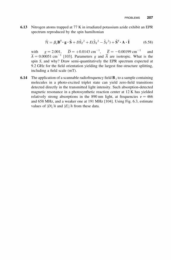
6.13 Nitrogen atoms trapped at 77 K in irradiated potassium azide exhibit an EPR

spectrum reproduced by the spin hamiltonian

H ¼ beBT� g � Sþ DSZ2 þ E(SX

2 � SY2)þ ST�A � I (6:58)

with g ¼ 2.001, D ¼ þ0.0143 cm21, E ¼ 20.00199 cm21 and

A ¼ 0.00051 cm21 [103]. Parameters g and A are isotropic. What is the

spin S, and why? Draw semi-quantitatively the EPR spectrum expected at

9.2 GHz for the field orientation yielding the largest fine-structure splitting,

including a field scale (mT).

6.14 The application of a scannable radiofrequency field B1 to a sample containing

molecules in a photo-excited triplet state can yield zero-field transitions

detected directly in the transmitted light intensity. Such absorption-detected

magnetic resonance in a photosynthetic reaction center at 12 K has yielded

relatively strong absorptions in the 890 nm light, at frequencies n ¼ 466

and 658 MHz, and a weaker one at 191 MHz [104]. Using Fig. 6.3, estimate

values of jDj/h and jEj/h from these data.

PROBLEMS 207

systems with more than one unpaired electron

Documents