systems of difference equations with general homogeneous boundary conditionsc) · 2018-11-16 ·...
TRANSCRIPT

SYSTEMS OF DIFFERENCE EQUATIONS WITH
GENERAL HOMOGENEOUS BOUNDARY CONDITIONSC)
BY
STANLEY OSHER
1. Introduction. As Strang [2], [3] has pointed out, a natural tool for studying
l2 stability of difference equations which approximate hyperbolic or parabolic
equations in one space variable is the Wiener-Hopf technique of factorization of
Toeplitz matrices discussed in [4] by Gohberg and Krein.
Strang has discussed stability of difference equations whose solutions satisfy the
special boundary condition u = 0 on and outside of the boundaries. We shall use
Toeplitz matrices to generalize this theory to systems of equations in one space
variable with arbitrary homogeneous boundary conditions. The discussion will be
confined to problems in the quarter plane with constant coefficients. The results
can be easily generalized to variable coefficient and two point boundary value
problems, using Kreiss' method [1] and/or Strang's in [2] and [3].
We shall derive Kreiss' sufficient conditions for stability of dissipative hyperbolic
systems with constant coefficients as a corollary to a more general result. In
particular, the condition of dissipativity is replaced by a weaker condition.
We treat the explicit case in the main part of this work and add the implicit case
as an appendix in part 7. The main results are stated in XIX and XXVIII. Kreiss'
Theorem is derived in XXII. We give nondissipative examples in XXIII and
XXIX.
We hope to extend this technique to include problems in several space variables
in the near future.
2. Basic problem. Consider a first order hyperbolic system of partial differential
equations
(2.1) ut = Aux, where A is a diagonal matrix with constant entries:
I, dx <0,d2 <0--dno <0,
J c/no+1 > 0, dno + 2 > 0- • -dp > 0.dj
Take the initial-boundary value problem in the quarter plane
(2.2) u(x, 0) =f(x);OSx<oo,
Received by the editors January 21, 1968.
0) This work performed under the auspices of the U.S. Atomic Energy Commission.
(dx
177
License or copyright restrictions may apply to redistribution; see https://www.ams.org/journal-terms-of-use

178 STANLEY OSHER [March
(2.3) u'(0, t) = S„u"(0, t), S„ is a rectangular constant (n0xp — n0) matrix.
U' = (M(1>(x,i),...,M<V(*,f)),
u" = (M("o + D(x, t ),..., u(p)(x,t)).
We approximate this system of partial differential equations by the system of
difference equations
(2.4) (a) v? + 1 = 2 Ckvï+k; j = s,s+l,...,n = 0,l,2,...(2)
with boundary conditions
(2.4) (b) vy1 = -'j? ai+x,k+xvnk + 1; y = 0, I,...,5-l,« = 0, 1,2,....k = s
r, 1, and s are nonnegative integers, vn is a p component vector:
dj = ^"(2)
-f?(p)j
The Ck are constant diagonal (p xp) matrices. The a,k are constant (p xp) matrices.
(We shall sometimes write a,_k for a,k.) vy = <£>, is a given arbitrary initial vector.
For simplicity, we define aJk = 8(j-k)I if 1 Sj, kSs, and thus equation (b) may be
rewritten
(2.4) (b') J «y+lifc+i»S+1 - 0, « = 0, l,...,j = 0, l,...,j-l.k = 0
Let u(x, t) be the solution to (2.1) with initial conditions (2.2) and boundary
conditions (2.3). We introduce a time step k>0 and a mesh-width «>0 and divide
the interval 0ax<co into subintervals of length «. Assume k/h = p = constant. Let
u(jh, nk) = ûf,
fi(jh) = ûf,
/ = 0,1,...,
« = 0,1,....
We say the difference scheme is a consistent approximation to the differential
equation if ûf satisfies 2.4(a) and 2.4(b) with a remainder which is of order 0(k2)
and <S>,=fi(jh) + 0(h2) for sufficiently smooth u(x, t) and/(x). Let us assume that
the difference scheme is indeed consistent with the basic system of differential
equations and boundary conditions.
(2) Notice that if s=0, the difference scheme is independent of the boundary conditions,
and Strang's necessary and sufficient conditions [2] are valid. Thus, we shall take s>0 and
C-s^[0]pXp.
License or copyright restrictions may apply to redistribution; see https://www.ams.org/journal-terms-of-use
1969] SYSTEMS OF DIFFERENCE EQUATIONS 179
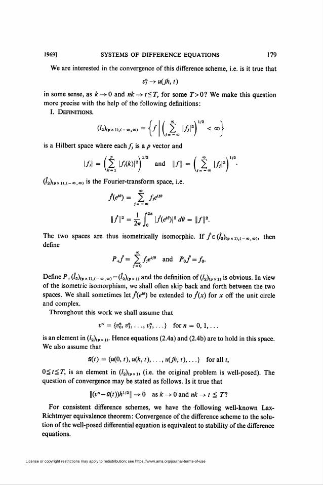
We are interested in the convergence of this difference scheme, i.e. is it true that
pjf -> u(jh, t)
in some sense, as k-+0 and nk-> tST for some F>0? We make this question
more precise with the help of the following definitions:
I. Definitions.
» ,1/2 -\
2œ \f\2) < œj
is a Hubert space where each/ is ap vector and
(P \ 1/2 / » \ 1/2
2j/A*)lj and ¡/I = ^ 2j/y|j ■
(4)(pxi),(-"c.,«o) is the Fourier-transform space, i.e.
f(eiB) = 2 #*i= -co
1 />2ji
ll/l|2=¿jo l/(0|8^= Il/Il'-
The two spaces are thus isometrically isomorphic. If /e(4)(pxi>,(-cx..a», then
define
V- 2fem and F0/ = /0.i = o
Define F+(/2)(pXl)>(_0O,a>) = (/2)(j>xi> and the definition of (/2)(pxl) is obvious. In view
of the isometric isomorphism, we shall often skip back and forth between the two
spaces. We shall sometimes let f(ew) be extended to f(x) for x off the unit circle
and complex.
Throughout this work we shall assume that
V = {vn0,vî,...,v],...} for« = 0,1,...
is an element in (/2)(p x u. Hence equations (2.4a) and (2.4b) are to hold in this space.
We also assume that
ü(t) = {u(0, t), u(h, /),..., u(jh, t),...} for all t,
OStST, is an element in (/2)(Pxi) (i.e. the original problem is well-posed). The
question of convergence may be stated as follows. Is it true that
||(7jn-i7(0)«1/2| -> 0 as k -> 0 and nk -> t S F?
For consistent difference schemes, we have the following well-known Lax-
Richtmyer equivalence theorem : Convergence of the difference scheme to the solu-
tion of the well-posed differential equation is equivalent to stability of the difference
equations.
(4)(pX l).(-OO.CO) '(
License or copyright restrictions may apply to redistribution; see https://www.ams.org/journal-terms-of-use

180 STANLEY OSHER [March
II. Definition. The difference equations (2.4a) and (2.4b) are said to be stable
if there exists a constant M>0 such that for any initial conditions v° = (f>¡ with
0 = {OO, $!,...}e(/2)(pxl) it follows that ||/jB||^iW||0|| for all n^O.
The basic problem of this work is in obtaining conditions on (2.4) which assure
its stability.
We may obtain consistent boundary conditions many different ways. For
example
vl + 1 = 2vV1-vn2f1
is consistent with any differential equation or boundary condition as may be
verified by merely examining the Taylor series
2û(sh, nk) = 2[w(0, nk) + ûx(0, nk)sh + ûxx(6x, nk)(sh/2)2],
û(2sh, nk) = û(0, nk) + ûx(0, nk)2sh + ûxx(62, nk)(2sh/2)2.
Consistency follows because k/h = constant. Clearly, we do not expect such trivial
boundary conditions to be appropriate regardless of the underlying partial differ-
ential equation. We shall discuss in another paper the question of appropriate
boundary conditions
III. Remark. The mapping of vn to vn +1 defined by the equations (2.4) is clearly
linear. That is, there exists a linear operator F such that vn+1=Lvn. This operator F
may be written as a finite-dimensional perturbation of a convolution operator
premultiplied by an orthogonal projection.
More precisely, we define
C(x)= 2 Ckx~kfc= -s
and recall
p+ 2/**'= 2¿*'' Po2fx'=f0,y =-<x> j = o j = o
««* Z(j-k)l if 1 Sj,kS s.
Then we may write L = T+S, where Tu(x)=P+C(x)u(x) defines the Toeplitz
operator, and
Su(x) = -2 ^o(2 x-kanx,k+xC(x)u(x));=0 \k=0 I
defines the finite-dimensional operator. Thus we may restate the basic problem.
Obtain conditions on the Ck and the ajk such that 3 a constant M > 0 with ||(F+ S)n||
S M for all «^0.
In what follows, we shall treat the question of stability independently of con-
sistency, unless otherwise stated. Thus, we shall concern ourselves with power-
boundedness of F+S and forget about the differential equations until we explicitly
mention them.
License or copyright restrictions may apply to redistribution; see https://www.ams.org/journal-terms-of-use

1969] SYSTEMS OF DIFFERENCE EQUATIONS 181
3. Preliminary stability theorem (Kreiss). We need an important stability
theorem which is a generalization of a result of H.-O. Kreiss [1].
IV. Lemma. Let L be a bounded linear operator on a Hilbert space H and P be an
orthogonal projection on H such that ||(7—P)L\\S 1.
Then for any <t> e H:
n
||FnO||2 S \m2+ 2 IIFF^H2.k = l
Proof.
||F<D||2= ||PF<D||2-|-||(/-P)FO||2
S ||FF<D|2+||0)||2 because \\(I-P)L\\ S 1-
Suppose the result is valid for LkQ>, k= 1, 2,..., n.
||Ln + 10||2 = || PLn + x <512+ || (I-P)LLn<S> ||2
S ||FFn + 1<D||2+||FnO||2
n
S ||PLn+^||2+ 2 ||FF'1«!)||2+1101|2. Q.E.D.k = l
V. Lemma. Let L be a bounded linear operator on H and P be an orthogonal
projection on H such that \\L(I—P)\\ S 1.
Then, for any 3> e H:
2 ||P(L(/-F))><D||2 S m2.1=0
Proof. We shall show that
"2 ||F(F(/-F)y<D||2+||(F(/-F))"<I)||2 S M21 = 0
by induction on n. For «= 1
||P<I>||2+||(/-F)<D||2 = ||(D||2
and ||L(/-F)01| = ||F(/-F)(/-F)0|| S ||(/-F)<D|| because (I-P) is idempotent and
||F(/-F)||^l.Thus
||FO||2+||F(/-F)0||2 S \M2.
The induction step is similar with (L(I—F))"0 used in place of O.
VI. Theorem. Let L be a bounded linear operator on a Hilbert space H. Let P
be an orthogonal projection on H. Assume
(1) ||(/-F)F||gl,
(2) \\L(I-P)\\Sl-
License or copyright restrictions may apply to redistribution; see https://www.ams.org/journal-terms-of-use
182 STANLEY OSHER [March
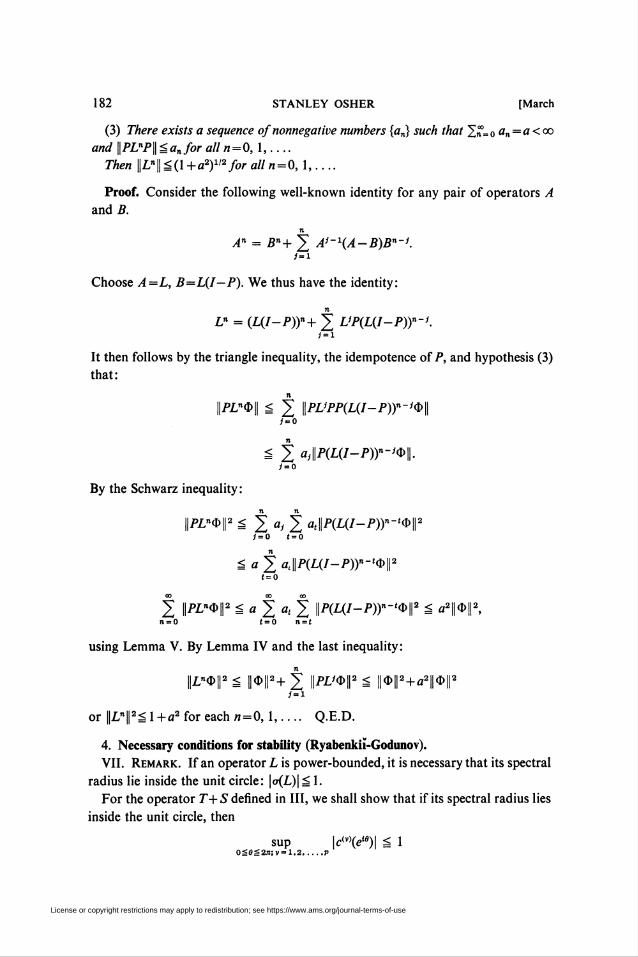
(3) There exists a sequence of nonnegative numbers {an} such that 2"= Oan = a<oo
and \\PLnP\\Sanfor all n = 0, 1,....
Then \\Ln\\S(l +a2)ll2for alln = 0, 1,....
Proof. Consider the following well-known identity for any pair of operators A
and F
An = Bn+ 2 Ai~1(A-B)Bn-i.
i=x
Choose A=L, B=L(I-P). We thus have the identity:
n
Fn = (L(I-P)f+ 2 LiP(L(I-P))n~i.i = i
It then follows by the triangle inequality, the idempotence of F, and hypothesis (3)
that:
n
||FFnO]| S 2 ||FFíFF(F(/-F))n-í0)||;' = o
n
S 2 ai\\P(L(I-P))n-1^\\.1 = 0
By the Schwarz inequality:
|FF"<D||2 S 2 a, 2 ^(FiF-F))"-^!!2Í = 0 Í = 0
S a 2 ai||F(L(/-P))»-«*||a(=0
CO CO CO
2 ||FFn<I>||2 S a 2 at 2 ||F(F(/-F))"-,*|a á a2||0||2,n=0 t=0 n=i
using Lemma V. By Lemma IV and the last inequality:
||F"4>||2 S ||«||a+2 ll^^ll2 = II$II2 + «2IIoII21=1
or ||Fn|[2^l+a2 for each « = 0, 1,.... Q.E.D.
4. Necessary conditions for stability (Ryabenkii-Godunov).
VII. Remark. If an operator F is power-bounded, it is necessary that its spectral
radius lie inside the unit circle: |<t(L)| S I.
For the operator F+ S defined in III, we shall show that if its spectral radius lies
inside the unit circle, then
sup \cM(eiB)\ S 1OS0S2ji;v = 1,2.p
License or copyright restrictions may apply to redistribution; see https://www.ams.org/journal-terms-of-use

1969]
where
SYSTEMS OF DIFFERENCE EQUATIONS
cm(x)
183
C(x) = 0 cM(x) 0
0 0 P"\x)-
Suppose we assume c(vo'(cl>o)=A0 and |A0| > 1. Let vN(j)=0 ifj^v0,
vN(vo) = -{0,0,...,0,e-t(r + s + l + »e0
,0,..
(The first nonvanishing term above is in the r+s+l+l place.) Then
|M = 1, yet ||(F+S-A0K||^0as/V-^co.
.'. A0 is in the spectrum of T+ S.
A0ea(F+5)and |A0| > 1.
Moreover, it follows easily that
||F|| S lo sup |c(vV)l S Fv = 1.2.P¡0á9g2JI
Consider F- A + 5" where A is a complex number and || F || S I < | A |. It is clear that
F—A is invertible. It is a well-known theorem e.g. [11] that if R is invertible and
S is finite dimensional, then R+S is invertible iff R+S annihilates no nonzero
vector.
We now have the following results : (a) => (b) o (c).
(a) T+S is power-bounded.
(b) \oiT+S)\Sl.(c) ||F||S1 and, if |A|>l,then(F+5,-A)M=0oM=0
7*11 S 1 o sup \cMiew)\ S 1).v = l,2.p;0á8S2ll )
It is not true in general that (c) => (a). For example consider the scalar difference
equation :
d}+1 = vf-lt /= 1,2,...,« = 0,1,...
with boundary conditions
vn0 + 1 = 2vnx + 1-vl + 1, « = 0,1,....
This is consistent with ut= -ux (OSt, x) for /c/« = l. C(eie) = ée; hence \T\Sl.
If (T+S-\0) 2f=o ̂ ,^=0, then \JV, = W,_X, j=l, 2,.... Thus Yy=<//AS for
some constant d and
J[l-2/A0+l/A2] = 0od = 0 and/or A0 = 1.
License or copyright restrictions may apply to redistribution; see https://www.ams.org/journal-terms-of-use

184 STANLEY OSHER [March
Thus condition (c) is verified. However, if we let v° = 0 if/>0 and v%=l, then
7j" = max (n—j+l, 0) and we, of course, have instability. We thus need additional
conditions to assure power-boundedness of T+S.
The condition that ||F|| S 1 is just the well-known von Neumann criterion which
is necessary for stability of pure initial value problems. The condition that
T+S should have no eigenvalues outside the unit circle is merely the additional
Ryabenkiï-Godunov condition which is needed for the mixed initial-boundary
problem, (see [12]).
In general, if |<r(L)|^l, then Ve>0 3k(e)>0 such that \\Ln\\Sk(e)(l +e)n.
We can show a stronger result for our difference operator F+ S:
If |o(T+ S)\Sl, then 3kx>0 and k2>0 such that
\\(T+S)n\\ S kxnk2.
We shall omit the proof of this result.
5. Resolvent of T+S.
VIII. Lemma. Let
(1) A be an invertibie operator,
(2) F be finite dimensional,
(3) (A + B)u = 0ou = 0.
Then (A + B)'1 exists and
(A + B)-1 = A-1 - A-^I+BA-^-^A-1.
Proof. We may show A + B is invertible by using the same well-known theorem
that we used in VII for R + S. We have the general identities for A and F in a non-
commutative algebra, A and A + B both invertible.
(A + B)-\A + B) = I
(A + BY^I+BA-1) = A-1
(A + B)-1 = A~1-(A + B)-1BA-1
= A-'-A-^I+BA-^-'BA-1.
IX. Corollary. If
(1) sup0S8aa»!ï=1.a.p|cnei0)|álo|lF]|^l,
(2) (T+S-\)xb = 0for |A| > 1 => xb = 0.
Then (T+ S-X)'1 exists and
(5.1) (T+S-X)-1 = (F-A)-1-(F-A)-1(/+5'(F-A)-1)-15'(F-A)-1.
Proof. In the last lemma, replace A by T- A and F by S.
X. Lemma and Definition. Suppose A is invertible and B is finite dimensional.
Then A + B fails to be invertible iff there exists a vector v in the range of B such that
v=-BA~1v.
Let || F || S I < |A|. Then, if we let D(X) be the finite-dimensional operator mapping
License or copyright restrictions may apply to redistribution; see https://www.ams.org/journal-terms-of-use

1969] SYSTEMS OF DIFFERENCE EQUATIONS 185
the range of S into itself:
(5.2) D(X)PS = PS + S(T-X)-1PS,
where Ps is the orthogonal projection onto the range of S, it follows that
(T+S-X)u = 0=>u = 0o \D(X)\ ï 0.
(We write \F\ for the determinant of the matrix F.)
Proof. A + B fails to be invertible iff there exists u^O such that (A + B)u = 0.
Let Au = v^0. Hence (I+BA~1)v = 0 or v=-BA~lv.
The second result follows if we substitute S for B and T— A for A.
XI. Remark. We now notice that the expression (5.1) for the resolvent of
r+ S may be rewritten
(5.3) (F+S-A)-1 = (F-A)-1-(F-A)"1[F)(A)]-1S(F-A)-1.
We shall obtain (F—A)-1 using the theory of Toeplitz matrices. We then shall
use this resolvent with (5.2) to obtain a matrix representation for the finite di-
mensional operator D(\). This gives us a simple expression for (T+S— A)-1. We
shall use the resolvent of F+ 5 as a generating function for the powers of T+ S, and
thus, with the help of Theorem VI, we shall obtain the stability conditions.
The following discussion of Toeplitz matrices contains only those elements of the
theory necessary for our work here.
XII. Lemma and Definition. Let
b(x) = b.sxs+ ■ • • +blx~\ î>0â -/, b.s # 0 # b,.
Then the Toeplitz operator on (l2)a x u defined by
Tbf=P+b(e^)f(e^)
is a bounded linear operator with norm
||rj S sup \b(eis)\.0S9S2JI
Moreover, suppose
(1) b(ew)^0, 0SBS27T and
(2) mdexoiBS2nb(eie) = 0.
It then follows that
(V) b(x) has the unique factorization b(x) = b^(x)b+(x), where
m*)- n(i -j), i Vii < i,/ = i,2,...,/,
s
b+(x) = b_s n (x-Xi), \.\i\ > 1, / = 1, 2,..., s;i = l
(flk, = 1 ifib < a\>
and hence 6_(x) is analytic and nomanishing for |.v|äl; b+(x) is analytic and
nonvanishing for \x\ S 1 ■
License or copyright restrictions may apply to redistribution; see https://www.ams.org/journal-terms-of-use
186 STANLEY OSHER [March
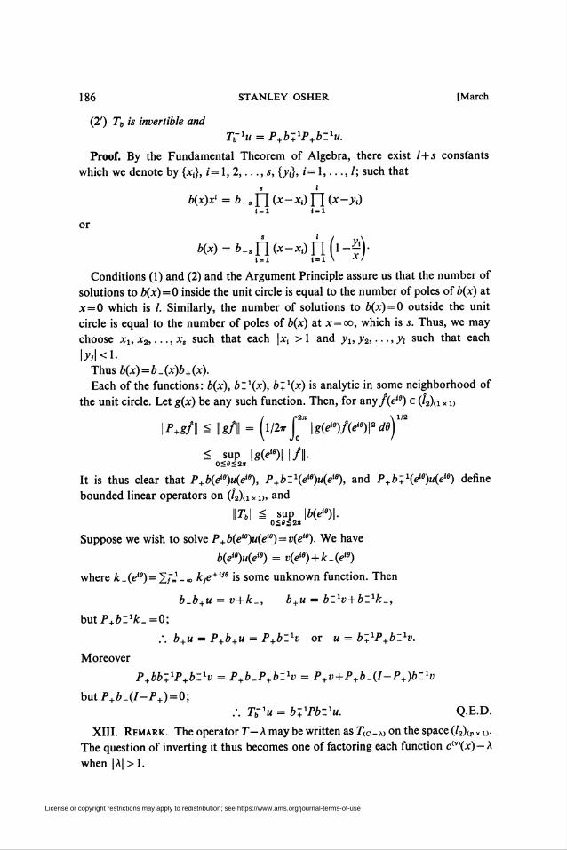
(2') Tb is invertible and
F,,"1« = P+bl1P+bZ1u.
Proof. By the Fundamental Theorem of Algebra, there exist l+s constants
which we denote by {x¡}, i=l, 2,..., s, {yt}, i=l,..., I; such that
b(x)xl = b.sfl(x-Xi)Yl(x-yi)1=1 i=i
or
b(x) = b„sYi(x-Xi)Yi(i-*\1=1 1=1 \ -*•/
Conditions (1) and (2) and the Argument Principle assure us that the number of
solutions to b(x) = 0 inside the unit circle is equal to the number of poles of b(x) at
x = 0 which is /. Similarly, the number of solutions to b(x) = 0 outside the unit
circle is equal to the number of poles of b(x) at x = oo, which is s. Thus, we may
choose Xi,x2,...,xs such that each |*¡|>1 and yx, y2, ■ ■ -, yt such that each
Thus b(x) = b _ (x)b+(x).
Each of the functions: b(x), bz1(x), b+1(x) is analytic in some neighborhood of
the unit circle. Let g(x) be any such function. Then, for any f(eie) e (/2)(1 x u
/ r2" \ 1'a
\\P+gf\\ = Ik/ll = (l/2»Jo \g(eie)f(eiT de)
S sup \g(e«)\ |/||.oses2)t
It is thus clear that P+b(ew)u(eie), P+èrVXe'9), and P+b-+\ëe)u(eiB) define
bounded linear operators on (/2)(1 M x), and
||rb|| S sup |/3(ei9)|.0S8S2JI
Suppose we wish to solve P+b(et0)u(eie) = v(ew). We have
b(ée)u(eiB) = v(eie) + k-(eie)
where A:_(ei9) = 2f=-» kje + m is some unknown function. Then
b-b+u = v + k_, b+u = bz1v + bz1k-,
butF+/3:1Â:_=0;
/. b+u = P+b+u = P+bZxv or u = bZ1P+bZ1v.
Moreover
P+bb+1P+bZlv = P+b_P+bzH = F+/;+F+/3.(/-P+)è:1t>
butP+è_(/-P+)=0;
.-. TÇ'u = bZ'Pbz'u. Q.E.D.
XIII. Remark. The operator F- A may be written as F(C-a> on the space (/2)(p » u.
The question of inverting it thus becomes one of factoring each function cw(x) - A
when |A| > 1.
License or copyright restrictions may apply to redistribution; see https://www.ams.org/journal-terms-of-use

1969] SYSTEMS OF DIFFERENCE EQUATIONS
XIV. Lemma. Let
187
P(x) = 2 Pix S = F-S*s+ • • • +Pi/x'i= -s
for sa — / have the property that
sup \p(ew)\ S 1.OS0S2JI
Fef X be a complex number such that \X\ > 1. Let p-s^0=^p¡. Then
(1) p(ew)-X¿0, OseS2tt and
(2) indexoSeS2Ap(ei0)-*]=0.
It then follows that
p(x)-x = q(X) n fv-^(a)) n (i -^V¡ = 1 i = l \ x I
Each |.Yj(A)| > 1, eac« |f¡(A)| < 1, and q(X) is a nonzero number which may depend
on A.
Proof. Since |/?(ei9)| < |A|, conditions (1) and (2) are immediate. We then apply
Lemma XII to b(x)=p(x) — X; the result then follows.
XV. Definition and Corollary. Let
sup |c(v)(eie)| S 1.0<9S2íi;v = 1.2.P
Let Xbe a complex number with \ X\ > 1. Then, by the last lemma, we may factor
p»(x)-x = dv(x) n (x-x\»(x)) n (i -^)-i=i i=i V x i
Each \x\v)(X)\ > 1, /= 1, 2,..., sv; each \y\v)(X)\ < 1, /= 1, 2,..., /v,
C<V)(X) = C(-V)SvA-s"+ • • ■ +C¡VV7.X\ ív = -/v,
c(-vi ̂ o ^ <#>.
F«e number dv(X) is a nonzero constant which may depend on X. Let
A-(x,X) =
ftfi-ffi) 00
0
0
0
A+(x, A) -ni = l
0
0
• ^(A)fK-v-Af'(A))
License or copyright restrictions may apply to redistribution; see https://www.ams.org/journal-terms-of-use

STANLEY OSHER [March
Then
C(eie)-X = A_(eie, X)A+(eie, X).
Thus, we may state as our main conclusion of this section:
(T-Xy^x) = Al\x, X)P+AZ\x, X)u(x).
Proof. This result follows in a straightforward way from the results of the last
three sections.
We have thus obtained the resolvent of F. We shall now obtain the matrix
F(A)FS defined in (5.2) and then use (5.3) to get the resolvent of T+S.
XVI. Definition and Lemma. Let sup |c<v)(c?i9)| S 1. Let X be a complex number
with |A| >1.
A + x(x, A) and A Z \x, X) have expansions
A + X(x, X) = 2 A(+{1))(X)xi convergent for \x\ < 1.J = 0
oo
AZ\x, X) = 2 A{I"^X)x~i convergent for \x\ > 1.
Let H(X) be the upper triangular matrix
«H(X) =
[0] [AI-&]
L [0]
Let & be the matrix of boundary conditions
"[ail][«l2] ■■■ [«i,r + s+i]
[a21][a22] • • •
.K.ilk-,2] ••• K.r + s + l]
[A-(s-iA
[A-(S-2)i
[A(-<U] j((sp)x(sp))
(sp)x((r + s+l)p)
Finally consider ¿é( A), which is a matrix consisting of the first (r + s+l)p compon-
ents of the sp linearly independent solutions to the problem
2 Ckvk+j = Xvj, j = s, s+l,..
This matrix is
sF(X) =
-[*;&] [0]
[^ + (1)] M + (0)]
-M + Cr + s)] U* + (r + s + l)]
[0] '
[0]
M+(0>]
MV-^i,].(((r + s+l)p)x(sp))
License or copyright restrictions may apply to redistribution; see https://www.ams.org/journal-terms-of-use

1969] SYSTEMS OF DIFFERENCE EQUATIONS
Now we may state our main results of this section :
F>(A)FS= -XF(X)H(X)PS,
189
where
F(A) = &s/(X).
Moreover \H(X)\ = 1, and |F>(Ao)|=0 iff |F(A0)| =0.
Proof. The first result is just a straightforward calculation. D(X) is the matrix
defined on the range of S by the operator
Fs + SFF-A)-^ = D(X)PS.s-l
Psf = 2 8}X} for some vectors g,(f).i = 0
Su= -2 ^o(2 x-ka,+ i¡k+i(C(x)-X))u(x);=0 \k=0 I
s-1 /r + s \
-A 2 x'Pol 2 x-kcc,+ i,k+iu(x)\-i=o \fc=0 /
Let u=(T-X)~1Psfi. The first term above becomes
-2 ^0(2 ^_s+1.fc+i) 2 g^ = -2 x'p0 2 2 xv-k8(j-k)gvi = 0 \k = 0 1 v = 0 J' = 0 v = 0fc = 0
= -2^= -psf-¡ = 0
Thus, the total is merely
-A 2 x'p/f x-ka,+ Xik+x)(T-X)-i 2^v3=0 \/c = 0 / v=0
= -A 2 ^Fo(2 x-ka,+x,k+x)A^P+Azi 2g,x\
where we have used the expression for (F—A)-1 which we derived in the last lemma.
It is clear that P+AZ1 is an analytic projection times an anti-analytic map and
hence is represented by an upper triangular matrix. In fact
P+A:»(2 gx) = 2 *" 2 Ai-»-^\v = 0 / u = 0 v = «
and thus the matrix of the transformation is
'[Al-(%] [A<S&] ••• [Al-dlvY
[0] [A^U]
L [0] [0] [AL-&] \(sp)x(sp)
H(X) =
which is upper triangular. Also AL^^Al^^I so \H(X)\ = l.
License or copyright restrictions may apply to redistribution; see https://www.ams.org/journal-terms-of-use

190 STANLEY OSHER [March
For arbitrary vectors of the form 25=o hjX1 we have:
s-l /r + s \ s-1
-A 2 X'P0[ 2 «"S+l.fc+lMï1 2 "^j = 0 \)c = 0 / i=0
s-l /r + s min(fc.s-l) \
--A^I^wt. 2 ̂ -TdV-iAJy = 0 \rC=0 i = 0 /
s-l s- 1 /r+s \
= -A 2 -^ 2 2 s+i.fc+i^-"("-())«(>1 = 0 t = 0 \k=t I
and the matrix of this transformation is thus —Xâstf(X)= —F(X)X. The total matrix
is -X&s?(X)H(X). We have thus shown that D(X)PS=-XF(X)H(X)PS. We have in
fact shown that
ß[/+S(F-A)-1]Ö= -AF(A)Fi(A)ß
where Q 2f=0 fix1=2)11 fxK Now
|ß(/+5(F-A0)-1)ß| =0
iff 3ßw^0 such that Qu= -S(T-X0)-1Qu. Hence Qu is in the range of S, or
Qu=Psu since QiPs- It is now clear that
|ß(/+5(F-A0)-1)ß| = 0o |F(A0)| = 0
and hence |F(A0)|=0 o |F(Ao)|=0. Q.E.D.
6. Sufficient conditions for stability (main theorems). We have thus obtained the
resolvent (T+S—A)-1 if |A|>1. We shall now state and prove two important
technical lemmas which are concerned with the analyticity in A of each of the
factors A + (x, X) and A^(x, A). Notice that each element in A + (x, X) and A_(x, X) is
essentially a symmetric function of the roots of a polynomial. Moreover, A appears
as a coefficient in this polynomial. We thus expect each factor to be an analytic
function of A.
The important condition in the next lemma is hypothesis (1). This condition will
be called "separation of the zeros". For |A| > 1, each of the solutions top(x) — X = 0
lies either well inside the unit circle (|,V((A)|<1) or well outside the unit circle
(l-x^A)! > 1). As A -> A0 with |A0| = 1, some of the zeros may approach the unit
circle, e.g. limA^Ao/7(x;(A)) = A0 for |A0| = |x;(A0)| = 1. Hypothesis (1) guarantees
that 3 no A0 on the unit circle such that, for some two zeros x,(X) and j¡(A), x;(A)
-> ji(A) as A -> A0, with |A| > 1.
XVII. Definition and Lemma. Fei p(x)=p-sxs+ ■ ■ ■ +p¡/xl be as in XIV.
Let |A|>l.Fei
m+(x,X)=q(X)fl(x-xl(X)\i=i
-(*,A) = n(i-^)i = l \ A '
License or copyright restrictions may apply to redistribution; see https://www.ams.org/journal-terms-of-use

1969] SYSTEMS OF DIFFERENCE EQUATIONS 191
be the factorization obtained in XIV. We say p(x) — X separates its zeros if there exists
a positive quantity 8 such that
l^(A)-v/A)| > S
for all | A | > 1 and all i,j.
We now assume
(1) p(x) — X separates its zeros.
(2) p(x) is not identically equal to a constant of absolute value one.
P(x) & Po where \p0\ = 1.
Then the following is true concerning the factors m+ and w_ :
(F) m + (x, A)/A is an analytic function of x and Xfior all x^co and l-d<\X\Soo,
d>0, and
Umm±ix1X)^_LA—w A
«i_(x-, A) is an analytic junction of x and X for x^O and 1— d<\X\S&>, and
limA^co «j_(x, A)=l.
(2') XmZ\x, A) is analytic if 1 -d< \X\ Sec and \x\ < 1 -d', d'>0.
mZ1(x, X) is analytic if 1 — d< |A| Soo and \x\ >l+d'.
Proof. The terms 1 —y{(X)/x and x,(X)—x are analytic in A for 1S |A| <oo except
perhaps for isolated algebraic branch points. Hence, if the functions
0(1-^) and fl(x-*,(A))
are single valued in A for co > | A| ̂ 1, then they are both analytic in A for oo > | A| = 1.
Consider a point A0 with co> |A0|_ 1. By hypothesis (1) we may take a circle F
in the A plane with center A0 and a sufficiently small radius so that
(6.1) |*.(A)-vy(A)| > 8/2
if A lies in this circle. The factor «i_ (x, A), for fixed x, is a symmetric function of the
roots Vi(A). • • v¡(A). Consider any smooth closed path in the A plane which lies
entirely within T. We choose any point À in this path and follow the value of j¡(A)
for each / around the path and back to À. Because of (6.1), it is clear that the values
of the v¡(A), /'= 1,2,...,/, will be at worst permuted among themselves. Thus, by
the symmetry of «i_(x, A), it follows that m_(x, A) is single valued in this neighbor-
hood of A0. The same reasoning works for I"I*-i (x-x,{X)). Of course d(X) is
analytic in A, and hence m+(x, X) is also analytic in this neighborhood of A0.
Now we examine the behavior of the factors near A = co. If/áO, then m_(x, X) = l.
If/>0, then Ve>0, consider the circle \x\ =e. We may choose X(e) so that
|A(£)| > sup \p(ee">)\.
License or copyright restrictions may apply to redistribution; see https://www.ams.org/journal-terms-of-use

192 STANLEY OSHER [March
Then p(x) — X(c) has index zero on the circle |x|«=«. Thus
\yi(X(e))\ < e, /'= 1,2,...,/.
Hence limA_„o «7_(.v, A)= 1 and we may show that /t7_(.y, A) is analytic and single
valued in A near A = co, using the same reasoning as we used in the last paragraph
about permuting thej¡(A). If s = 0, then «7 + (.v, A) = —X+pQ. If s<0, then /?7 + (a', A)
= — A. If j>0, then VoOwe may take
|~(1/*)| > SUp \p((lle)-F%-n<0Sit
Thenp(x)— ^(l/e) has index zero on the circle \x\ = l/e and hence
\Xj(t(l/e))\ > l/e, j=l,2,...,S.
Thus m + (x, X) is single valued near A = oo and has a pole at A = oo. Hence we now
have:
m+(x, X) = dj(x)k'+dJ.i(x)X'-1+- • -,
m-(*,A)- i+^M+....
If we match coefficients of A in the equation «7_»7+ =p(x) — X we obtain j=l and
d](x)= — 1. We thus have proven conclusion (V). Conclusion (2') would follow
immediately from the analyticity of m+(x, A)/A and m_(x, X) if we knew that each
factor was nonsingular in the regions described in (2'). It is clear that
n(l™r) and fl(x-x,(A))¡=i\ x¡ i=1
are both nonsingular in the respective regions. The constant q(X) is independent of A
unless sSO. If s<0, q(X)=-X. If s = 0, then q(X)= -X+p0. By hypothesis (2), if
l=0=s, then \p0\ <1. If/>0, then
p(x)-X = (-X+pQ)Ù(l-^y \yi(X)\Sl,i=l,2,...,l \X\i\.
and if \p0\ i 1, then p(x)=p0, which is a contradiction. Thus q(X) is nonsingular in
the proper region. The result (2') is now immediate.
We may now use these results in an obvious way in order to obtain analyticity in
A of A + (x, A), A _(x, A), F(A), and their inverses.
XVIII. Lemma. Suppose
sup |c(v)(c?i9)| S 1v = 1.2,...,p;OS0S2Jl
We make the following two assumptions:
(I) For each v, the zeros ofciv)(x) — X are "separated" in the sense defined in the
License or copyright restrictions may apply to redistribution; see https://www.ams.org/journal-terms-of-use

1969] SYSTEMS OF DIFFERENCE EQUATIONS 193
last definition and lemma. That is, there exists a positive quantity 8 such that
|.ySv'(A)-j<v)(A)| > 8 forall\X\ > 1 and alii, j, v.
(2) For each v, cM(x) is not identically equal to a constant of absolute value one,
c(v,(x)Mv) for |4V,| = 1.
Then the quantities A + (x, A), A_(x, A), A + 1(x, A), Az1(x, X) and F(X) (which were
defined in XV and XVI) have the following properties:
(V) A + (x, A)//A is an analytic matrix function of x and X for all x#co and 1 — d
< \X\ Sco for some d>0 and
lim A + (x,X)I/X = -I.A-*oo
A_(x, X) is an analytic matrix function of x and Xfior all x^O and 1 — d< \ X\ S oo
í7«í/limAJ0O A-(x, X) = I.
(2') XIA + !(x, X) is analytic in both variables if 1—í/<|A|^oo and \x\<l—d',
d'>0.
Az1(x, X) is analytic in both variables if 1 — d< \X\ ¿oo and \x\ >l+d'.
(3') XIF(X) is analytic //coa |A| > 1 -dandlim^ A/F(A)= -/.
Proof. This is an immediate corollary of the last lemma and of the definitions of
these quantities. Q.E.D.
We may now proceed to prove our main theorem. We do this without requiring
that 2.4 be consistent with the P.D.E. (2.1). The strategy we shall use is as follows:
(1) We apply Theorem VI to L = T+S, with F being the projection onto the first
r + l+s components of a vector in (l2\pxi).
(2) Assumptions (1) and (2) of that theorem are immediately verified since
(I-P)S=S(I-P) = 0 and ||r||gl.
(3) We use the resolvent (5.1) in Lemma IX in order to verify condition (3). This
operator will be used as a generating function:
(F+S-A)-i=-2 (I¿^ for |A| > 1.n = 0 n
XIX. Main Theorem. Suppose
(1) SUPv=1>2.p;-,<aS3I|c(Ve)l=l.
(2) For each v the zeros of cM(x) — X are separated as defined in XVII. That is,
there exists a positive quantity 8 such that \x^\X)—yy"\\)\ >8for all \X\ > 1, and all
i,j, »■
(3) For each v, c{v)(x) is not identically equal to a constant of absolute value one,
C(v)(.v)^C(oV)H77/í |CÍ)V)| = 1.
(4) |F(A)|^0 for oo>|A| = l. (Recall |F(A)|= determinant of F(X) and F(X)
= a¿/(X).) Then 2.4 is stable.
Proof. We apply Theorem VI to L = T+S. Let
r + l + s/co \ r + l+s
p[2fn= 2 »*\; = 0 / 1 = 0
License or copyright restrictions may apply to redistribution; see https://www.ams.org/journal-terms-of-use
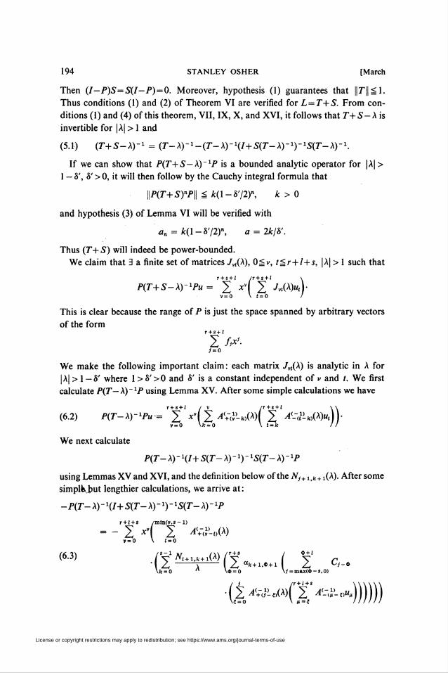
194 STANLEY OSHER [March
Then (I-P)S=S(I-P) = 0. Moreover, hypothesis (1) guarantees that ||F||^1.
Thus conditions (1) and (2) of Theorem VI are verified for L = T+S. From con-
ditions (1) and (4) of this theorem, VII, IX, X, and XVI, it follows that T+S- X is
invertible for |A| > 1 and
(5.1) (T+S-Xy1 = (T-X)-1-(T-X)-1(I+S(T-X)-1y1S(T-X)-1.
If we can show that P(T+S— A)_1F is a bounded analytic operator for |A| >
1 — 5", 8' >0, it will then follow by the Cauchy integral formula that
■ || P(T+S)nP || S k(l-8'/2)\ k>0
and hypothesis (3) of Lemma VI will be verified with
,an = k(l-h'/2)n, a = 2k/8'.
Thus (T+ S) will indeed be power-bounded.
We claim that 3 a finite set of matrices Jvt(X), O^y, tSr + l+s, \X\ > 1 such that
r + s + l /r + $ + l \
P(T+S-X)~1Pu = 2 *v 2 ^(A)«, •v=0 \ (=0 /
This is clear because the range of F is just the space spanned by arbitrary vectors
of the formr + s+i
2 />*'•1 = 0
We make the following important claim: each matrix Jn(X) is analytic in A for
|A| > 1 — 5' where 1 > S' >0 and 8' is a constant independent of v and /. We first
calculate P(T—X)~1P using Lemma XV. After some simple calculations we have
(6.2) PCT-Xy^u = r2+'W2 A^lk)(X)(+f AL-JLk)(X)u\\v=0 \k=0 \ t=k II
We next calculate
P(T- X) - l(I+ S(T- X) - !) - XS(T- X) - lP
using Lemmas XV and XVI, and the definition below of the Nj+ x¡k+ X(X). After some
simplKbut lengthier calculations, we arrive at:
-P(T- A) - X/+ S(T- X) - !) - 'SÇT- X) - !P
r + l + s /mln(v.s-l)
= - 2 W 2 ^(+-<?-o(A)v=0 \ i=0
\lc = 0 " \» = 0 \y = max(«-s,0)
'(2/*«"»(A)(l'^"-»"-))))))
License or copyright restrictions may apply to redistribution; see https://www.ams.org/journal-terms-of-use

1969] SYSTEMS OF DIFFERENCE EQUATIONS 195
where we have defined the matrices Nt+XJ+x(X) for OSl, jSs—l and |A|>1 as
follows:
-ia^ =F-\X)
[Nxx(X)]pxp ■■• [Nlt],
LU»sl]pxp [/*ss]p (sp X sp)
Conditions (1), (2), (3) and Lemma XVIII assure us that each XA^uftX) and
^(_~("(A) is analytic in A for 1-</< |A|2oo. Condition (4) and the same lemma
assure us that each Af(+lifc+1(A)/A is analytic in A for 1 — d" < |A|s¡oo, d" >0. Hence,
using (5.1), (6.2) and (6.3), each /vt(A) is a finite linear combination of products of
matrices which are analytic for 1 —8'<|A|áoo, 1 > S' > 0. Thus the analyticity of
each ./„¡(A) follows.
Stability is now immediate. Q.E.D.
We shall now compare our results with those of H.-O. Kreiss [1]. In fact we shall
obtain his main result for the constant coefficient case as a corollary to our main
theorem. We first make his assumptions. In particular, we notice that he assumes
consistency with the partial differential equation and boundary conditions (2.1),
(2.2) and (2.3). Moreover, he needs the restriction of dissipativity. We have
essentially replaced these conditions by requiring that c(v)(x) not be a constant of
absolute value one and by our condition of "separation of zeros", or "positive
distance between zeros". We shall show that our conditions are more general. We
shall also give a nondissipative example for which stability may be verified by using
our main theorem.
Assumptions. (1) The difference equations (2.4a) and (2.4b) are consistent with
the hyperbolic system of partial differential equations (2.1), (2.2) and (2.3).
(2) 3 no nontrivial solution to (2.4) of the form
CO
vn = AS«/., for |A0| > 1 and 2 W < °°-1 = 0
(3) The difference approximation is dissipative, i.e. 38 >0 and a natural number
t > 0 so that
\cM(eie)\ S l-8\d\2t forv= l,2,...,p.
XX. Lemma (Kreiss). If assumptions (I), (2) and (3) are valid, it then follows that
3e with 0<e< 1 3 for any As |A| > 1 :
(a) For 1 SjSn0, 3 no vP(A) with 1 -eS | vP(A)| S 1,
(b) For «o + l SjSp, 3 no x\n(X), with 1S |*r°(A)| £ 1+«.
(c) If |A| = 1 and A^l then 3 no xl'XX) or y\i}(X) of absolute value one. For
j= 1, 2,..., «0, there exists exactly one i(j) such that |x{fj)(I)| = 1, in fact x[(),)(l)= 1.
For j=«0+l, ...,p, there exists exactly one i(j) such that | v!u>(l)| = l, in fact
(d) c(v)(x) is not a constant for each v.
License or copyright restrictions may apply to redistribution; see https://www.ams.org/journal-terms-of-use

196 STANLEY OSHER [March
These properties clearly imply that the zeros are separated.
Proof. See Kreiss [1, Lemmas 6 and 7].
XXI. Lemma. Suppose assumptions (1), (2) and (3) are valid. In addition, equation
(2.4) has no nontrivial solution of the form v] = AnXFy with \X\ = 1 and
(a) ir=o|lF;|2<oo//A/l.
(b) WlSk, \Y'/\Skp\ifX=l;j=0,l,...with 0Sp<l and k>0. It then follows that \F(X)\ /0 for any X with |A| = 1.
Proof. If |F(Ao)|=0, then 3 a nontrivial eigenvector g with F(A)g=0. Let h¡,
j=0, 1,..., s—l, be defined by
g = [[«o](P x l)["l](P x 1)' • • l"(s-l)](pxl)](sp xl).
LetmlnO'.s- 1)
% = 2 A^ik)(x)hk.k-0
It then follows by using the definition of F(A0) that
r+s
2 oti+l.» + lT» = 0, j = 0,1,..., S-l.u = o
We claim
2 Yyx* = A-y(x, A0)'2 hkxk1=0 k=0
is a nontrivial solution to (T+SyY(x) = X0Y(x) but T(x) may not be an element of
(/2)(pXi). This is true because the general solution to the problem
¡2 Ckuj+k = Xuj, j = s,s+l,...
fc= -s
for |A| > 1, in (/2)(pxi) is a linear combination of the solutions to
P+x-s[C(x)-X]Y(x) = 0.
Let y¥(x) = 2îZh x'A+Kx, \)h„ then
P+x-s[C(x)-X]xiA~+1(x, X) = P+x'-'AzHpc, A) = 0 if; < s.
We now let A ->- A0. We already know that
r + s
2 «y+i.c + iY# = °» j=* 0,1,...,s-l« = o
for A = A0. Because of the continuity of each /^""(A) for |A| > 1 -d, it is clear that
2 CkyVj+k -> AqT, as A -> A0, j = s,s+l,....It»-a
The claim is thus proven.
License or copyright restrictions may apply to redistribution; see https://www.ams.org/journal-terms-of-use

1969] SYSTEMS OF DIFFERENCE EQUATIONS 197
We shall now estimate the coefficients
A?>(A0), y = 0,1,....
If A0#l, then by conclusion (c) of the last lemma, 3^'(A0) with 0<|u'(A0)< 1 such
that
|l/xP(A0)| ¿M'(A0) for all/,/
This implies that Y(x) is in (/j),,,,,. If A0 = l, then 3p' with 0<p'<l such
that ¡l/x^Xl^Sr1' for all i if j=n0+ 1, «0 + 2,.. .,p; and for all / but one excep-
tional i(j) for each /= 1, 2,..., «0, and x$,(l)=l for this /(/). It then follows
that
\vlj\sk, \vy\*W, 7 = 0,1,...
for A:>0 and 0<p< 1.
Thus vn = XlYj has the properties forbidden in the hypothesis and hence |F(A)|
=«=0 if |A| = 1. Q.E.D.
XXII. Theorem (Kreiss). Suppose assumptions (I), (2), and (3) are valid.
Assume equation (2.4) has no nontrivial solution of the form vn, = An<I>; with \X\ = l and
(a) 2r=o 10,|2<oo (FA^l.
(b) |<DJ| <k, \<&'/\Skp'ifX=l andj=0, 1,... with 0Sp< 1 and k>0.Then (2.4) is stable.
Proof. We must merely verify the conditions of Theorem XIX. This verification
is immediate from the assumptions, the last two lemmas, Lemma X, and Lemma
XVI.
XXIII. Example. Consider the hyperbolic P.D.E. in the quarter-plane
ut = ux, x, fäO u(x, 0) = Q>(x). Take the difference approximation
u? + 1 = l+£un+i + l^£un_it y= 1,2,...,« = 0,1,...
M = -r—> 0 < p < 1
mS+1 =2mî + 1-«3 + 1, « = 0,1,2,...,
»r1-»? = n. nr»?+i-«?i. /i_ nr«?-«?-iiAi \2p 2J[ ¿sx J \2 2/x/L Ax J
= Mx(yAx,«A?) + 0(Ar), MS + 1-2wï + 1 + mS + 1 = 0((Af)2).
Thus we have consistency.
C(ew) = cos 0-/*/sin 6
\C(ew)\ = [l+Oi2-l)sin20]1/2 S 1 ifO < p< 1.
ia^)i = 1.
License or copyright restrictions may apply to redistribution; see https://www.ams.org/journal-terms-of-use

198 STANLEY OSHER [March
Thus the approximation is not dissipative, so we cannot use Theorem XXII.
However
C(x)-X = ?(x-Xlix))(i-yf)
-(^i/x-x+^y
Hence
|*i(A)*(A)| = ({$*) > 1 or l*i(A)| > l/bi(A)|
for |A|2:1. Thus the zeros are separated. Moreover,
Al1(x,X)= -2/1-/* J
hence
ih (*i(A)y+i*
F(A) = -2/(l-p)xx(X)[l-2/xx(X)+l/x2x(X)].
If F(Ao) = 0 for oo > |A0| i 1, then X!(A0)= 1. This is a contradiction.
We thus have stability. Q.E.D.
7. Appendix—Implicit difference equations. The apparatus we have set up in
the previous sections in order to handle the stability theory of explicit difference
schemes may be modified to include implicit difference approximations to (2.1).
See [13] for a thorough description of the implicit case. In this appendix we shall
discuss some of the highlights of the stability theory of implicit difference equations.
The difference approximation is of the form
i i(7.1)(a) 2 B*VW= 2 CkVl+i, j=s,s+l,...,n = 0, 1,...,
k= -s k= —s
with boundary conditions-
r+s r+s
(7.1)(b) 2 «/+i.fc+i°S+l - 2 »+1.-+!* 7 = 0,1,...,1-1,11-0,1,.:.,fc=0 fc=o
where i>0 and [C_s]^[0].
The Bk and Ck are again diagonal (p xp) matrices, ajk and yik are again (pxp)
matrices,
\ba\x) 0
and
B(x)= 2 Bkx~k =
C(x) = 2 Ckx-k =
0
-ca)(x)
0
bw(x).
0 -
àp\x).
License or copyright restrictions may apply to redistribution; see https://www.ams.org/journal-terms-of-use

1969] SYSTEMS OF DIFFERENCE EQUATIONS 199
Moreover, we assume that each bu\x) has as many zeros inside the unit circle
counting multiplicity as it has poles at ,r=0. (See [13] for an explanation of this
last assumption.)
We notice that if (1) t=s, (2) yjk = 0, (3) Bk = 8(k)I, (4) ajk = 8(,_k)I for OSj,
kSs— 1 ; then this problem reduces to the explicit case.
XXIV. Remark. Equation (7.1) may be rewritten on (/2)<Pxd as
(T0 + S0)v« + 1(x) = (Tx + Sx)v»(x).
F0 and Tx are again Toeplitz matrices; SQ and Sx are again finite-dimensional
operators :
T0vn + 1 = P+xt-sB(x)vn + 1(x),
Txvn = P+xl-sC(x)vn(x),
t-l r r + s
S0vn+1 = 2 x'Po -x-'"-°B(x)+2 «,+1>k+;*1=0 L k = 0
SiV* = J X'P0 -X-' + t~*C(x)+ 2 Yi+x.k+xXkn+x.k+x^1=0 L k=o
vn + 1(x),
vn(x).
We thus wish to obtain
(a) necessary and sufficient conditions for (Tq + So)'1 to exist, and
(b) sufficient conditions so that || [(F0 + S0) ' \TX + Sx)]n \\ S M for all n= 0, 1,....
XXV. Theorem. The following conditions are necessary and sufficient for the
operator T0 + S0 to be invertible on (/2)(p x 1} :
(1) bw(eiB)¿0for v=l, 2, ...,p; Oá 6S2rr,
(2) t = s,
(3) (T0 + S0)v=0ov=0.
We now assume throughout that (Fo + S'o)"1 exists.
XXVI. Remark. Condition (a) => (b) o (c); but (c), in general, does not imply
(a).
(a) (To + Sr^-^Ti + Sj) is power bounded.
(b) \o((T0+SQ)-HTi+Si))\£l.
(c) supv = lt2.p:0SeS2, \qw(e,e)\Sl where qw(x) = F»(x)/b™(x)
and(Ti + Sx-X(T0 + S0))v = Ofor |A|>1 <>v = 0.
Moreover, condition (b) implies that 3kx, k2>0 such that
||[(F0 + 5o)-1(Fl + 51)r|| S kxnk2
XXVII. Definition. We may use the results of XII in much the same way as in
XV to factor
C(x)-XB(x) = A.(x, X)A + (x, A) for |A| > 1
License or copyright restrictions may apply to redistribution; see https://www.ams.org/journal-terms-of-use

200
such that
STANLEY OSHER [March
(Fi-AFo)-1!/ = Az\x, X)P+AZ\x, X)u.
We may then define the matrix s/(X) as in XVI. Let
= [y-AâK(A);— A
where
y-Xstf =
[yxx-Xaxx][yX2-XaX2]
[y21-Aa21][y22-Ao:22]
[ysi-^asi][ys2-^as2]
Lyi.r + s+l — Aai,r+s+lJ
[V2.r + s+l — A«2,r + s+l]
lys,r + s+l ^as,r + s + l]
XXVIII. Main Theorem (Implicit Case). The following conditions are sufficient
for stability :
(1) SUPv=1,2.P;0S9S2JI|?(V)(^)|=1.
(2) For each v, c(v)(x) — Xblv)(x) separates its zeros in the same way as p(x) — X did
in XVII.
(3) For each v, cw(x)/bw(x)^pl0n, where |/?0V)| = 1.
(4) |F(A)|^0/oroo>|A|=l.
XXIX. Example. Approximate the scalar hyperbolic P.D.E. in the quarter
plane x, f=-0:
Ui = ux with u(x, 0) = O(x)
by the implicit difference scheme
ur'-pßu^l+pßu^l = "?+i+ "?-!, j = l, 2,..., « = 0, 1,...,
(m=ä7o<4
and boundary conditions
"0 = 2unx + 1-uV\ « = 0,1,..
Consistency, invertibility, and stability may be easily verified for this non-
dissipative implicit example.
The author would like to thank Dr. A. Chorin for suggesting the idea upon which
this work is based and for participating in many interesting discussions relating to
it; Professor H.-O. Kreiss for asking incisive questions; Professor G. Strang for
valuable discussions on the implicit case and related topics; and Professor P. D.
Lax for graciously giving much time and patience in directing the research and for
contributing many ideas to the final result.
License or copyright restrictions may apply to redistribution; see https://www.ams.org/journal-terms-of-use

1969] SYSTEMS OF DIFFERENCE EQUATIONS 201
Bibliography
1. Heinz-Otto Kreiss, "Difference approximations for the initial-boundary value problem
for hyperbolic differential equations," in Numerical solutions of nonlinear partial differential
equations, Edited by D. Greenspan, Wiley, New York, 1966, pp. 141-166.
2. G. Strang, Wiener-Hopf difference equations, J. Math. Mech. 13 (1964), 85-96.
3. -, Implicit difference methods for initial-boundary value problems, J. Math. Anal.
Appl. 16 (1966), 188-198.
4. I. C. Gohberg and M. G. Krein, Systems of integral equations on a half line with kernels
depending on the difference of arguments, Amer. Math. Soc. Transi. 14 (1960), 217-288.
5. R. D. Richtmyer, The stability criterion of Godunov and Ryabenkii for difference schemes,
A.E.C. Research and Development Report NYO-1480-4, 1964.
6. Peter D. Lax and Burton Wendroff, On the stability of difference schemes, Comm. Pure
Appl. Math. 15 (1962), 363-371.
7. R. D. Richtmyer, Difference methods for initial value problems, Interscience, New York,
1957.
8. S. K. Godunov and V. S. Ryabenkii, Spectral criteria for the stability of boundary-value
problems for non-selfadjoint difference equations, Uspehi Mat. Nauk 18 (1963), no. 3(111), 3-15.
9. -, Canonical forms of systems of linear ordinary difference equations with constant
coefficients, Z. Vycisl. Mat. i Mat. Fiz. 3 (1963), 211-222.
10. -, Theory of difference schemes, an introduction, North-Holland, Amsterdam,
1964.
11. N. Dunford and J. T. Schwartz, Linear operators, Part 1, Interscience, New York,
1958.
12. S. J. Osher, Systems of difference equations with general homogeneous boundary conditions,
Brookhaven National Laboratory Report, BNL 11246, 1967.
13. -, Stability of mixed implicit difference schemes, Brookhaven National Laboratory
Report, BNL 11784, 1967.
Brookhaven National Laboratory,
Upton, L. I., New York
License or copyright restrictions may apply to redistribution; see https://www.ams.org/journal-terms-of-use