systemic risk estimation under dynamic volatility matrix

1

Systemic Risk Estimation under Dynamic Volatility Matrix Models

1Chuan Hsiang Han

This version: 11/15/2017

.

1. Department of Quantitative Finance, National Tsing-Hua University, Hsinchu, Taiwan 30013, R.O.C., E-mail:

[email protected]. Work supported by MOST 105-2115-M-007-012-MY2, Taiwan. We are grateful for Kaiyu Yang on

empirical analysis and Yenan Chen for importance sampling implementation.

2

Title: Systemic Risk Estimation under Dynamic Volatility Matrix Models

Abstract: This paper proposes a two-step procedure for systemic risk estimation under the stochastic

volatility/correlation models. The first step utilizes Fourier transform method for dynamic volatility matrix

estimation, and the second step develops efficient importance sampling estimators for extreme event

probability. For the empirical analysis, we find that the systemic risk can be useful to measure the stability of

financial system because it seems be able to provide early signs for institutions in U.S. during the 2008-2010

financial crisis. Moreover, it can serve as a predictor of the capital injections during the crisis. SRISK in China

and Taiwan are also compared.

Keywords: dynamic volatility matrix model, Fourier transform method, importance sampling, systemic risk.

3

Section 1: Introduction

After the 2008 financial crisis, systemic risk has become a theme of studies for the financial stability.

According to the definition from IMF, FSB, and BIS1 in 2011, systemic risk is “a risk of disruption to

financial services that is caused by an impairment of all or parts of the financial system, and can have serious

negative consequences for the real economy.” The European Central Bank (ECB) in 2010 defines the

systemic risk as “a risk of financial instability so widespread that it impairs the functioning of a financial

system to the point where economic growth and welfare suffer materially.” Fouque and Langsam (2013)

provide a working definition for systemic risk as “the risk of a disruption of the market’s ability to facilitate

the flows of capital that results in the reduction in the growth of the global GDP.”

Bisias et al. (2012) provide a survey on the systemic risk measures and conceptual frameworks that have

been developed over the past few years. There appear 31 quantitative measures of systemic risk in the

economics and finance literature. These research methods are categorized by five systemic risk measures

including probability distribution measures, contingent-claim and default measures, illiquidity measures,

network analysis measures, and macroeconomic measures. These five categories and their related systemic

risk measures are briefly described below.

CategoryⅠ Probability Distribution Measures: Perhaps one simple and direct measure of systemic

risk is the total sum of negative outcomes of a collection of important financial institutions. Acharya et al.

(2017) propose systemic expected shortfall (SES) to measure each financial institution’s contribution to

systemic risk. Furthermore, Acharya et al. (2012) introduces SRISK to measure the contribution of individual

1 IMF: International Monetary Fund

FSB: Financial Stability Board

BIS: Bank of International Settlement

4

financial institution to the whole systemic risk. Several factors are considered into SRISK such as firm’s size,

leverage and conditional expected shortfall. All these factors are used to differentiate contribution level of

financial institutions. Adrian and Brunnermeier’s (2016) propose conditional value at risk (CoVaR) which

measures the VaR of the system conditional on one institution being at its VaR with the same quantile. The

CoVaR systemic risk measure can identify the risk contribution of an individual institution on the system.

CategoryⅡ Contingent-Claim and Default Measures: Based on Merton’s structure model (1973), it

is possible to construct measures of default likelihood for each institution and connect them either directly or

indirectly through their joint distribution. This approach of contingent-claims analysis (i.e., derivatives pricing

models) is taken by Capuano (2008), Gray and Jobst (2010), and Huang et al. (2009a).

CategoryⅢ Illiquidity Measures: Illiquidity is an example of a highly specific measure of systemic

risk that often requires considerable structure. Khandani and Lo (2011) propose two distinct measures of

equity market liquidity, one of which is the profitability of an equity mean-reversion strategy, and the other is

a more direct measure of price impact based on Kyle (1985). Getmansky, Lo, and Makarov (2004) propose

using serial correlation as a proxy for illiquidity. Aikman (2010) has developed its risk assessment model for

systemic institutions to simulate the possibilities and point out that funding troubles can apply to both

traditional intermediaries as well as shadow banks.

Category Ⅳ Network Analysis Measures: Kritzman et al. (2010) use principal components analysis

to gauge the degree of commonality among a vector of asset returns, which is a way of network analysis

measures. Using Granger-causality test statistics for asset returns to define the edges of a network of financial

institutions are becoming popular. Billio et al. (2010) show that Granger-causality networks are highly

5

dynamic and become densely interconnected prior to systemic shocks.

CategoryⅤMacroeconomic Measures: The opposite of the theoretical probability-distribution

measures are the macroeconomic models of systemic risk. Reinhart and Rogoff (2009) provides comparisons

of broad macroeconomic aggregates such as asset price indices (equities, housing, etc.), GDP growth rates,

and public debt over many financial crises, and find a number of common patterns. Alessi and Detken (2009)

construct simple yet early-warning indicators from a broad range of real and financial indicators including

GDP and its components, inflation, interest rates, and monetary aggregates for 18 OECD2 countries between

1970 and 2007. Borio and Drehmann (2011) propose a related approach, but with signals defined by

simultaneous extreme values for pairs of property prices, equity prices, and credit spreads.

In this paper, our research is based on the systemic risk measure proposed by Acharya et al. (2012) in

CategoryⅠ Probability Distribution Measures. One innovation is applying the continuous-time dynamic

volatility matrix models to estimate the capital shortfall and provide a systemic risk indicator for financial

firms. The dynamic volatility matrix model (Malliavin and Mancino (2009), Mancino et al.(2017)) can

represent the behavior of financial returns from the perspective from the non-parametric estimation. This

facilitates the estimation of stochastic volatility/correlation models, which are known for capturing some

stylized features of financial data (Fouque et al. (2011)). Those models have been intensively applied to

derivative’s pricing and hedging issues based on option price approximation. While these approximations are

instrumental in reducing computational cost, there is still room of improvement for estimation accuracy.

Distinct from previous studies, we choose to value exact computation and incorporate the help of refined

2 the Organisation for Economic Co-operation and Development

6

efficient simulation method for more accurate estimation to avoid approximation errors. We propose an

improved procedure for systemic risk estimation with dynamic volatility matrix models under the historical

(or physical) probability measure by the following two steps: (1) dynamic volatility matrix model estimation

scheme by the Fourier transform method (Malliavin and Mancino (2009), Mancino et al.(2017)), and (2)

enhanced importance sampling for estimating extreme capital shortfalls.

For the first step, the non-parametric Fourier transform method to estimate dynamic volatility matrix

under continuous semi-martingale models is introduced. This method makes the estimation feasible and robust

by relying on the integration of the time series based on the computation of Fourier coefficients of the variance

process (Mancino (2017)). Some case studies for estimating instantaneous or spot volatility can be seen in

Han (2013).

For the second step, importance sampling is developed for the estimation issues of the tail areas (McNeil

et al. (2005)) when its problem is impossible to admit a close-form solution under complex dynamic volatility

matrix models. Importance sampling can effectively improve convergence of sample means particularly in

rare event simulation while direct Monte Carlo simulation suffers pitfalls like variance augmentation and slow

convergence (Glasserman (2003), Lemieux (2009)). We further propose an enhanced version of importance

sampling for estimating extreme event probability. The theoretical background of our proposed importance

sampling combines the large deviation theory (Bucklew (2004)) which has the averaging effect on the

homogenized system (Han (2012)) and provides a sharp estimate for the decay rate of small probabilities. This

methodology is useful in handling the heavy (or fatter) tail distributions induced by stochastic

volatility/correlation models.

7

We use this methodology to analyze the systemic risk of top financial firms in US, Taiwan and China

between 2005 and 2016. The SRISK analysis shows that pre-crisis SRISK is a predictor of the capital

injections performed by the Fed during the crisis and that an increase in aggregate SRISK provides an early

warning signal of a decline in industrial production.

The organization of this paper is as follows. Section 2 introduces the parameter estimation for dynamic

volatility matrix estimation. Section 3 reviews the Fourier transform method, one of the nonparametric

approaches to estimate volatilities and correlations in time series. Section 4 discusses the construction of the

efficient importance sampling estimators for extreme capital shortfall. Section 5 investigates backtesting

results of systemic risk estimation of China, Taiwan, and U.S., then we conclude in Section 6.

Section 2: Systemic Risk Estimation under Dynamic Volatility Matrix Models

Acharya et al. (2012) introduce SRISK as the expected capital shortfall of a financial institution

conditional on a prolonged market decline. The conditional capital shortfall(CS) is measured by the size of

the firm, its degree of leverage, and its expected equity loss conditional on the market decline. This measure

can be computed using the balance sheet information and an appropriate Long Run Marginal Expected

Shortfall(LRMES) estimator. SRISK is used to construct rankings of systemically risky institutions: Firms

with the highest SRISK are the largest contributors to the undercapitalization of the financial system in times

of distress. The sum of SRISK across all firms is used as a measure of overall systemic risk in the entire

financial system. It can be thought of as the total amount of capital that the government would have to provide

to bail out the financial system in case of a crisis.

8

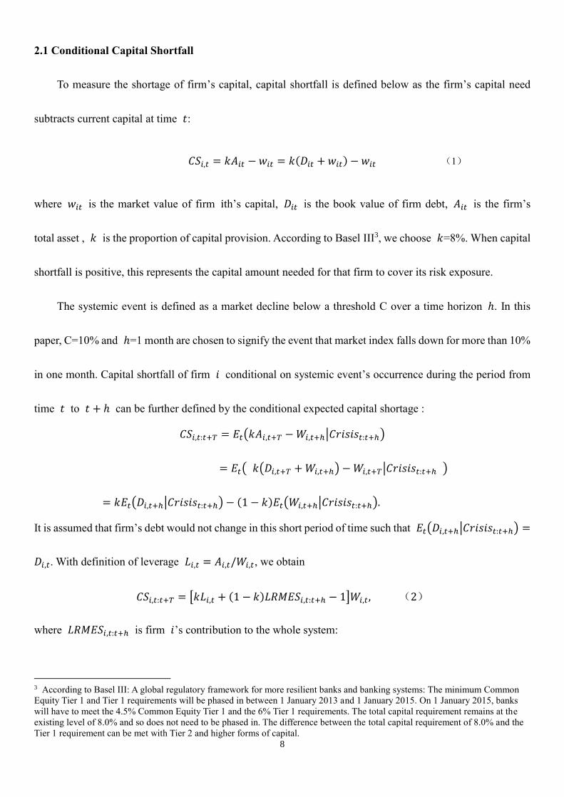
2.1 Conditional Capital Shortfall

To measure the shortage of firm’s capital, capital shortfall is defined below as the firm’s capital need

subtracts current capital at time 𝑡:

𝐶𝑆𝑖,𝑡 = 𝑘𝐴𝑖𝑡 − 𝑤𝑖𝑡 = 𝑘(𝐷𝑖𝑡 + 𝑤𝑖𝑡) − 𝑤𝑖𝑡 （1）

where 𝑤𝑖𝑡 is the market value of firm ith’s capital, 𝐷𝑖𝑡 is the book value of firm debt, 𝐴𝑖𝑡 is the firm’s

total asset , 𝑘 is the proportion of capital provision. According to Basel III3, we choose 𝑘=8%. When capital

shortfall is positive, this represents the capital amount needed for that firm to cover its risk exposure.

The systemic event is defined as a market decline below a threshold C over a time horizon ℎ. In this

paper, C=10% and ℎ=1 month are chosen to signify the event that market index falls down for more than 10%

in one month. Capital shortfall of firm 𝑖 conditional on systemic event’s occurrence during the period from

time 𝑡 to 𝑡 + ℎ can be further defined by the conditional expected capital shortage :

𝐶𝑆𝑖,𝑡:𝑡+𝑇 = 𝐸𝑡(𝑘𝐴𝑖,𝑡+𝑇 −𝑊𝑖,𝑡+ℎ|𝐶𝑟𝑖𝑠𝑖𝑠𝑡:𝑡+ℎ)

= 𝐸𝑡( 𝑘(𝐷𝑖,𝑡+𝑇 +𝑊𝑖,𝑡+ℎ) −𝑊𝑖,𝑡+𝑇|𝐶𝑟𝑖𝑠𝑖𝑠𝑡:𝑡+ℎ )

= 𝑘𝐸𝑡(𝐷𝑖,𝑡+ℎ|𝐶𝑟𝑖𝑠𝑖𝑠𝑡:𝑡+ℎ) − (1 − 𝑘)𝐸𝑡(𝑊𝑖,𝑡+ℎ|𝐶𝑟𝑖𝑠𝑖𝑠𝑡:𝑡+ℎ).

It is assumed that firm’s debt would not change in this short period of time such that 𝐸𝑡(𝐷𝑖,𝑡+ℎ|𝐶𝑟𝑖𝑠𝑖𝑠𝑡:𝑡+ℎ) =

𝐷𝑖,𝑡. With definition of leverage 𝐿𝑖,𝑡 = 𝐴𝑖,𝑡/𝑊𝑖,𝑡, we obtain

𝐶𝑆𝑖,𝑡:𝑡+𝑇 = [𝑘𝐿𝑖,𝑡 + (1 − 𝑘)𝐿𝑅𝑀𝐸𝑆𝑖,𝑡:𝑡+ℎ − 1]𝑊𝑖,𝑡, （2）

where 𝐿𝑅𝑀𝐸𝑆𝑖,𝑡:𝑡+ℎ is firm 𝑖’s contribution to the whole system:

3 According to Basel III: A global regulatory framework for more resilient banks and banking systems: The minimum Common

Equity Tier 1 and Tier 1 requirements will be phased in between 1 January 2013 and 1 January 2015. On 1 January 2015, banks

will have to meet the 4.5% Common Equity Tier 1 and the 6% Tier 1 requirements. The total capital requirement remains at the

existing level of 8.0% and so does not need to be phased in. The difference between the total capital requirement of 8.0% and the

Tier 1 requirement can be met with Tier 2 and higher forms of capital.

9

𝐿𝑅𝑀𝐸𝑆𝑖,𝑡:𝑡+ℎ = -𝐸𝑡 {𝑊𝑖,𝑡+ℎ

𝑊𝑖,𝑡− 1|𝐶𝑟𝑖𝑠𝑖𝑠𝑡:𝑡+ℎ} （3）

≈1

𝑁∑ [

−∑ 𝑟𝑖,𝑡,𝑡+ℎ 𝐼(𝑟𝑀,𝑡:𝑡+ℎ<𝐶)#

∑ 𝐼(𝑟𝑀,𝑡:𝑡+ℎ≤𝐶)#

]𝑁𝑠=1

where 𝐼(𝑥) = 1 when 𝑥 is true and 0 otherwise, 𝑟𝑀,𝑡:𝑡+ℎ and 𝑟𝑖,𝑡,𝑡+ℎ are returns of the market index and

firm 𝑖 during the period from 𝑡 to 𝑡 + ℎ, respectively. 𝐿𝑅𝑀𝐸𝑆𝑖,𝑡:𝑡+ℎ is often estimated by Monte Carlo

method.

Lastly, firm 𝑖’s systemic risk is defined as a positive capital shortfall:

𝑆𝑅𝐼𝑆𝐾𝑖,𝑡:𝑡+𝑇 = (0, 𝐶𝑆𝑖,𝑡:𝑡+𝑇)+ .

The aggregated systemic risk 𝑆𝑅𝐼𝑆𝐾𝑀,𝑡:𝑡+𝑇=∑ (0, 𝐶𝑆𝑖,𝑡:𝑡+𝑇)+

𝑖 can be used as a measure of the injection from

the government. Individual financial firm’s contribution to the system is defined as the ratio below:

𝑆𝑅𝐼𝑆𝐾%𝑖,𝑡:𝑡+𝑇=𝑆𝑅𝐼𝑆𝐾𝑖,𝑡:𝑡+𝑇

𝑆𝑅𝐼𝑆𝐾𝑀,𝑡:𝑡+𝑇⁄ （4）

2.2 Parameter estimation for volatility models

In order to estimate LRMES, an appropriate model is in need to compute the expected market return and

each firm’s return. There are a number of methods that can be used to estimate. GARCH-DCC model use by

Acharya et al. (2012) is a discrete-time parametric method to estimate correlation matrix of multi-asset returns.

Similar dynamic models can be found in continuous time. For example, one can use Heston model to simulate

stochastic volatility and assume that stochastic correlation follows Jacobi process.

2.2.1 Discrete-time model: GARCH-DCC

Dynamic conditional correlation model is a kind of multivariate model proposed by Engle (2002). It is

defined as:

10

1/2

2 ' 2

1 1 1

1

' '

1 1 1

1 1

,

z ,

,

{ } { } { } ,

~ (0, ),

,

{ } { }

t t t

t t t

t t t t

t i i t t i t

t t t t

t t t t

t t t t

r u

H

H D R D

D diag diag r r diag D

D N R

Q S A B A B Q

R diag Q Q diag Q

Where is a vector of ones and ° is the Hadamard product of the matrices. 𝜔𝑖,𝜅𝑖,λ𝑖 are the GARCH

parameters.

The other notations are as follow:

𝑟𝑡: n × 1 vector of log returns of assets at time 𝑡.

ξ𝑡: n × 1 vector of mean-corrected returns of 𝑛 assets at time 𝑡. E[𝑎𝑡] = 0.

Cov[𝑎𝑡] = 𝐻𝑡

𝜇𝑡: n × 1 vector of the expected value of the conditional 𝑟𝑡, which can be modelled as a constant

vector or a time series model.

𝐻𝑡: n × n matrix of conditional variances of 𝛼𝑡 at time 𝑡. 𝐻𝑡1/2

may be obtained by a Cholesky

factorization of 𝐻𝑡.

𝐷𝑡: n × n diagonal matrix of conditional standard deviations of 𝛼𝑡 at time 𝑡.

𝑅𝑡: n × n conditional correlation matrix of 𝛼𝑡 at time 𝑡.

𝑧𝑡: n × 1 vector of i.i.d. errors such that E[𝑧𝑡] = 0, E[𝑧𝑡𝑧𝑡𝑇] = 𝐼.

S: n × n unconditional covariance matrix of the standardized errors.

The GARCH-DCC model can be estimated in the following two step. In the first step, the conditional

heteroscedasticity is estimated by GARCH model. The second step is to estimate the correlation parameters.

The Maximum Likelihood Estimation(MLE) is used. With the parameters of GARCH-DCC, we can calculate

the SRISK with the simulation returns.

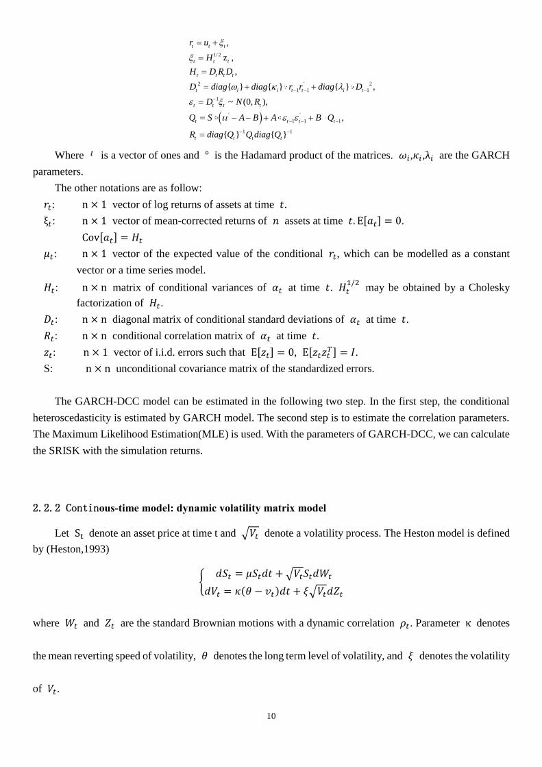
2.2.2 Continous-time model: dynamic volatility matrix model

Let St denote an asset price at time t and √𝑉𝑡 denote a volatility process. The Heston model is defined

by (Heston,1993)

{𝑑𝑆𝑡 = 𝜇𝑆𝑡𝑑𝑡 + √𝑉𝑡𝑆𝑡𝑑𝑊𝑡

𝑑𝑉𝑡 = 𝜅(𝜃 − 𝑣𝑡)𝑑𝑡 + 𝜉√𝑉𝑡𝑑𝑍𝑡

where 𝑊𝑡 and 𝑍𝑡 are the standard Brownian motions with a dynamic correlation 𝜌𝑡. Parameter κ denotes

the mean reverting speed of volatility, 𝜃 denotes the long term level of volatility, and 𝜉 denotes the volatility

of 𝑉𝑡.

11

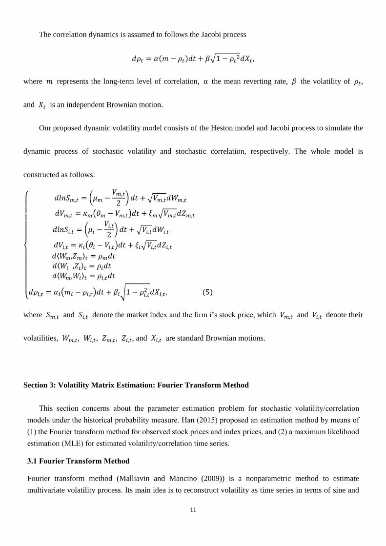
The correlation dynamics is assumed to follows the Jacobi process

𝑑𝜌𝑡 = 𝛼(𝑚 − 𝜌𝑡)𝑑𝑡 + 𝛽√1 − 𝜌𝑡2𝑑𝑋𝑡,

where 𝑚 represents the long-term level of correlation, α the mean reverting rate, 𝛽 the volatility of 𝜌𝑡,

and 𝑋𝑡 is an independent Brownian motion.

Our proposed dynamic volatility model consists of the Heston model and Jacobi process to simulate the

dynamic process of stochastic volatility and stochastic correlation, respectively. The whole model is

constructed as follows:

{

𝑑𝑙𝑛𝑆𝑚,𝑡 = (𝜇𝑚 −

𝑉𝑚,𝑡2) 𝑑𝑡 + √𝑉𝑚,𝑡𝑑𝑊𝑚,𝑡

𝑑𝑉𝑚,𝑡 = 𝜅𝑚(𝜃𝑚 − 𝑉𝑚,𝑡)𝑑𝑡 + 𝜉𝑚√𝑉𝑚,𝑡𝑑𝑍𝑚,𝑡

𝑑𝑙𝑛𝑆𝑖,𝑡 = (𝜇𝑖 −𝑉𝑖,𝑡2) 𝑑𝑡 + √𝑉𝑖,𝑡𝑑𝑊𝑖,𝑡

𝑑𝑉𝑖,𝑡 = 𝜅𝑖(𝜃𝑖 − 𝑉𝑖,𝑡)𝑑𝑡 + 𝜉𝑖√𝑉𝑖,𝑡𝑑𝑍𝑖,𝑡

𝑑⟨𝑊𝑚,𝑍𝑚⟩𝑡 = 𝜌𝑚𝑑𝑡

𝑑⟨𝑊𝑖 ,𝑍𝑖⟩𝑡 = 𝜌𝑖𝑑𝑡

𝑑⟨𝑊𝑚,𝑊𝑖⟩𝑡 = 𝜌𝑖,𝑡𝑑𝑡

𝑑𝜌𝑖,𝑡 = 𝛼𝑖(𝑚𝑖 − 𝜌𝑖,𝑡)𝑑𝑡 + 𝛽𝑖√1 − 𝜌𝑖,𝑡2 𝑑𝑋𝑖,𝑡, (5)

where 𝑆𝑚,𝑡 and 𝑆𝑖,𝑡 denote the market index and the firm i’s stock price, which 𝑉𝑚,𝑡 and 𝑉𝑖,𝑡 denote their

volatilities, 𝑊𝑚,𝑡, 𝑊𝑖,𝑡, 𝑍𝑚,𝑡, 𝑍𝑖,𝑡, and 𝑋𝑖,𝑡 are standard Brownian motions.

Section 3: Volatility Matrix Estimation: Fourier Transform Method

This section concerns about the parameter estimation problem for stochastic volatility/correlation

models under the historical probability measure. Han (2015) proposed an estimation method by means of

(1) the Fourier transform method for observed stock prices and index prices, and (2) a maximum likelihood

estimation (MLE) for estimated volatility/correlation time series.

3.1 Fourier Transform Method

Fourier transform method (Malliavin and Mancino (2009)) is a nonparametric method to estimate

multivariate volatility process. Its main idea is to reconstruct volatility as time series in terms of sine and

12

cosine basis under the following continuous semi-martingale assumption. Let 𝑢𝑗𝑡 be the log-price of an

underlying asset price 𝑆𝑗 at time 𝑡, so that 𝑢𝑗𝑡 = ln(𝑆𝑗𝑡), and follow a diffusion process

𝑑𝑢𝑗𝑡 = 𝜇𝑗𝑡𝑑𝑡 + 𝜎𝑗𝑡𝑑𝑊𝑗𝑡,

where 𝜇𝑗𝑡 is the instantaneous growth rate, 𝜎𝑗𝑡 is the instantaneous volatility, and 𝑊𝑗𝑡 is a one-dimensional

standard Brownian motion. Note that the original time interval can always be rescaled to so

that the Fourier transform of 𝑢𝑗(𝑡) can be defined by ∀ 𝑘 ∈ 𝑍,

𝔉(𝑢𝑗)(𝑘) =1

2 𝜋∫ 𝑢𝑗(𝑡)𝑒

−𝑖𝑘𝑡2𝜋

0

𝑑𝑡

=𝑖

𝑘[1

2𝜋(𝑢𝑗(2𝜋) − 𝑢𝑗(0)) − 𝔉(𝑑𝑢𝑗)(𝑘)].

The last equality is derived from the integration by parts. The new notation 𝔉(𝑑𝑢𝑗)(𝑘) is defined by

𝔉(𝑑𝑢𝑗)(𝑘) ≡1

2𝜋∫ exp(−𝑖𝑘𝑡)𝑑𝑢𝑗𝑡

2𝜋

0

.

Given two functions Φ and Ψ, the Bohr convolution product is defined as

(Φ ∗𝐵 Ψ)(𝑘) = lim𝑁→∞

1

2𝑁 + 1∑ Φ(𝑠)Ψ(𝑘 − 𝑠)

𝑁

𝑠=−𝑁

.

Malliavin and Mancino (2009) proved that in frequency domain, the Fourier coefficient of the (i,j)-th

instantaneous volatility matrix Σ(𝑡) is

1

2𝜋𝔉(Σ𝑖,𝑗)(𝑘) = (𝔉(𝑑𝑢𝑖) ∗𝐵 𝔉(𝑑𝑢𝑗)) (𝑘), 𝑓𝑜𝑟 𝑎𝑙𝑙 𝑘 ∈ 𝑍(In probability) (6)

Therefore, the instantaneous volatility matrix Σ(𝑡) can be calculated by the inverse Fourier transform

Σ𝑖,𝑗(𝑡) = 2𝜋 𝔉−1 ((𝔉(𝑑𝑢𝑖) ∗𝐵 𝔉(𝑑𝑢𝑗)) (𝑘)). (7)

Equation (7) reveals that given a set of spot price data {𝑆𝑖𝑡, 𝑆𝑗𝑡} under the historical probability measure, its

instantaneously volatility {Σ𝑖,𝑗(𝑡)} can be estimated by the Fourier transform method. Taking the financial

system described by equation (5) as an example : Σ𝑚,𝑖(𝑡) = 𝜎𝑚(𝑡)𝜎𝑖(𝑡)𝜌𝑖,𝑡 , where 𝜎𝑚(𝑡) = √𝑉𝑚,𝑡

and𝜎𝑗(𝑡) = √𝑉𝑗,𝑡 Note that 𝜎𝑖2(𝑡) = Σ𝑖,𝑖(𝑡) denotes the instantaneous variance process of the i-th asset and

[0,T] [0,2 ]p

13

2𝜋 𝔉(Σ𝑖,𝑗)(0)=∫ Σ𝑖,𝑗(𝑡)2𝜋

0𝑑𝑡 is equal to the integrated cross-volatility (Mancino et al.(2017)).

3.2 Parameter estimation for stochastic volatility/correlation model

Once instantaneous volatility and correlation are estimated by Fourier transform method, we can further

estimate parameters (𝜅, 𝜃, 𝜉) of the volatility process and (α,𝑚, β) of the correlation process via the MLE

from the discretized stochastic differential equations (Han (2013)):

�̂� =1

𝛥𝑡[1 −

𝑡 (∑𝑉𝑡+1𝑉𝑡

𝑡𝑖=1 ) − (∑ 𝑉𝑡+1

𝑡𝑖=1 )(∑

1𝑉𝑡

𝑡𝑖=1 )

𝑡2 − (∑ 𝑉𝑡𝑡𝑖=1 )(∑

1𝑉𝑡

𝑡𝑖=1 )

]

𝜃 =−1

�̂�𝛥𝑡[(∑

𝑉𝑡+1𝑉𝑡

𝑡𝑖=1 ) (∑ 𝑉𝑡

𝑡𝑖=1 ) − 𝑛(∑ 𝑉𝑡+1

𝑡𝑖=1 )

𝑡2 − (∑ 𝑉𝑡𝑡𝑖=1 )(∑

1𝑉𝑡

𝑡𝑖=1 )

]

𝜉 = √1

𝑛𝛥𝑡∑

1

𝑉𝑡[𝑉𝑡+1 − (�̂�𝜃𝛥𝑡 + (1 − �̂�𝛥𝑡)𝑉𝑡)]

2𝑡

𝑖=1

Parameter estimation for Jacobi process can be derived in the same way:

�̂� =1

𝛥𝑡[

1 −

∑1

1 − 𝜌𝑡2 ∑

𝜌𝑡+1𝜌𝑡1 − 𝜌𝑡

2𝑛−1𝑡=1 −𝑛−1

𝑡=1 ∑𝜌𝑡

1 − 𝜌𝑡2

𝑛−1𝑡=1 ∑

𝜌𝑡+11 − 𝜌𝑡

2𝑛−1𝑡=1

∑1

1 − 𝜌𝑡2

𝑛−1𝑡=1 ∑

𝜌𝑡2

1 − 𝜌𝑡2

𝑛−1𝑡=1 − (∑

𝜌𝑡1 − 𝜌𝑡

2𝑛−1𝑡=1 )

2

]

�̂� =1

�̂�𝛥𝑡[ ∑

𝜌𝑡1 − 𝜌𝑡

2∑𝜌𝑡+1𝜌𝑡1 − 𝜌𝑡

2𝑛−1𝑡=1 − ∑

𝜌𝑡+11 − 𝜌𝑡

2𝑛−1𝑡=1 ∑

𝜌𝑡2

1 − 𝜌𝑡2

𝑛−1𝑡=1

𝑛−1𝑡=1

(∑𝜌𝑡

1 − 𝜌𝑡2

𝑛−1𝑡=1 )

2

− ∑1

1 − 𝜌𝑡2

𝑛−1𝑡=1 ∑

𝜌𝑡2

1 − 𝜌𝑡2

𝑛−1𝑡=1 ]

�̂� = √1

(𝑛 − 1)𝛥𝑡∑

[𝜌𝑡+1 − (�̂� �̂�𝛥𝑡 + (1 − �̂�𝛥𝑡)𝜌𝑡)]2

(1 − 𝜌𝑡2)

𝑛−1

𝑡=1

,

14

For a simulation study, we set model parameters to simulate the market index and the firm i's share price

path, and then through the MLE method aforementioned to estimate those model parameters. Model

parameters are set as follows:

[INSERT TABLE 1 ABOUT HERE]

Figure 1 shows the simulated market index, the simulated volatility of the individual stock and the

volatility estimated by the Fourier method. Figure 2 shows that a simulated correlation in comparison with the

correlation estimated by the Fourier transform method.

[INSERT FIGURE 1 ABOUT HERE]


Section 4: Importance Sampling: Variance Reduction

When dealing with sparse observations in the tails, the basic Monte Carlo simulation suffers some

undesirable properties such as large relative error and data clustering around the center, etc. Importance

sampling is suitable for rare event simulation by improving the convergence of the basic Monte Carlo method.

The fundamental idea behind importance sampling is relocating the original density function to incur more

occurrences of rare events so that accurate estimates for small probabilities can be achieved. See Bucklew

(2004) for discussions on importance sampling and extreme event probability estimation and Han et al. (2014)

for applying importance sampling to the VaR/CVaR estimation problem under stochastic volatility model.

Based on the large deviation theory (Bucklew (2004)), an importance sampling estimator is

15

asymptotically optimal or efficient when the decay rate of its variance is zero in an asymptotic sense. When a

practical model appears to be complex, the asymptotic analysis doesn’t seem a plausible approach. One can

homogenize the system model (Han (2012)), then study the variance decay rate for the proposal importance

sampling (Han et al. (2014)). If the asymptotic optimality of the homogenized system model is assured, the

corresponding importance sampling is often effective to estimate capital shortfalls for complex systems.

4.1 Systemic Risk

We provide an application for estimating the systemic risk in the financial market. Define the LRMES

from time t to t + h by:

(8)

where 𝑟𝑀,𝑡:𝑡+ℎ and 𝑟𝑖,𝑡:𝑡+ℎare the return of market index and firm 𝑖 during the period 𝑡 to 𝑡 + ℎ.

In equation (8), Monte Carlo method can be used to simulate and the estimate LRMES. Since the market

“Crisis” is considered as a rare event, importance sampling can be feasible to reduce sample variance.

Following the same argument in Han et al. (2014), first homogenization then probability measure change, we

can derive the same importance sampling algorithm for estimating LRMES by virtue of large deviation theory.

4.2 Numerical Examples

We estimate LRMES under the complex dynamic volatility matrix model described in section 2. The

“barrier” style (hitting time) problem is consider and their numerical results are recorded on in Table 2.


From the numerical results, it is observable that the proposed importance sampling reduces the standard error

16

dramatically so that estimation for LRMES and SRISK become more accurate. The variance reduction ratios

for the constant cases and the stochastic volatility/correlation cases are 5~10 and 20~500 respectively.

Section 5: Data and SRISK measurement: US, Taiwan, and China

Our empirical analysis mainly focuses on financial institutions in the USA. Financial institutions which

have market value larger than 5 billion dollars are included in our sample for the period from Jan. 4th, 2005

to Dec. 1st, 2016. Open data such as daily log price, market value of each firm, its quarterly book value of

equity and debt are incorporated for calculating SRISK.

Sample firms are divided into four parts: Depositories (e.g., JP Morgen, Citi), Broker-dealers (e.g.,

Goldman Sachs, Morgen Stanly); Insurance (e.g., AIG); Others (e.g., Fannie Mae, Freddie Mac). Table 3

records the name and ticker of each selected firm. S&P 500 is chosen to represent the market index for

measuring SRISK.

5.1 SRISK Measurement

We calculate daily SRISK for all sample companies from January 2005 to December 2016. SRISK in the

form of moving window, using the calculation of previous half year's data, so our follow-up SRISK results

are with no forward-looking error. To calculate LRMES, we need to first estimate each company's Heston

model and the Jacobi process parameters with the relevance of the stock price. As a result of moving the form

of the window, each company's parameter estimates will also change.


17

5.2 SRISK’s Evolution and Ranking

CASE 1: U.S.

Figure 4 illustrates the SRISK of each sector during the period from July 2005 to December 2016.

Compared with S&P 500 index, one observes a strongly negative correlation between the total sum of SRISK

and S&P 500 index.


Table 4 specifies the proportion of the top ten financial systems with the highest systemic risk at the

beginning of the third quarter of the sample period and the overall systemic risk. Among them, the 2014-2016

ranking has a 0% risk ratio, indicating that the market risk of the existence of the system is limited, and the

overall systemic risk is low.


From July 2005 to July 2007, the overall financial system of the US is around $200 billion. In this figure

we can observe that most of the systemic risk are from the Broker sector. Among this sector, the biggest

contributors are Goldman Sachs, Morgan Stanly, Bear Stearns and Lehman Brothers. It is noteworthy that

these companies have played an important role in the subsequent global financial crisis, and as early as 2005

their systemic risks emerge while S&P 500 index was still arising. At the same time, the second highest

systemic risk comes from the 'Other' sector mainly contributed by Fannie Mae and Freddie Mac. Both

18

contribute a sum of about 20% of the overall systemic risk.

Since July 2007, the impact of subprime mortgage crisis to the overall system becomes more and more

apparent. Stock prices start to shake down and SRISK begins to accelerate. The composition of SRISK

changes gradually since then. With the crisis’s deepening and proliferation, the banking sector and the

insurance sector have also becoming an important SRISK contributors. Some large commercial banks also

appear on table 4(the TOP10 SRISK list), such as Bank of America, Citigroup, Wells Fargo and AIG.

In September 2008, the bankruptcy of Lehman Brothers raised the overall SRISK to achieve a peak.

Stock prices began to plummet and at this point, the contribution of banks and insurance to the overall SRISK

kept increasing. Top 5 SRISK contributors in the Q3 quarter of 2009 included the Bank of America, Citigroup,

Wells Fargo, JP Morgan and AIG. Many of the companies with higher SRISK rankings were missing from the

rankings. For example, Lehman Brothers went bankrupt in September 2008, Fannie Mae and Freddie Mac

were government-managed, and Bear Stearns was acquired by JP Morgan in March 2008.

The financial system has been steadily stabilizing since the second half of 2009 by the aid of three

consecutive quantitative easing (QE). SRISK has been reduced and the market has recovered. Although the

European debt crisis during 2010-2011 is a bump along the way. Figure 5 shows the SRISK changing for some

broker or depository companies.


CASE 2: China and Taiwan

Except SRISK in US, we choose Taiwan and China as an alternative study case and compare their

19

SRISKs.4

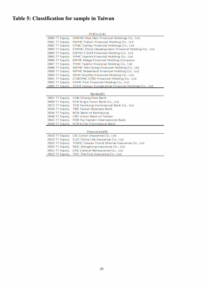
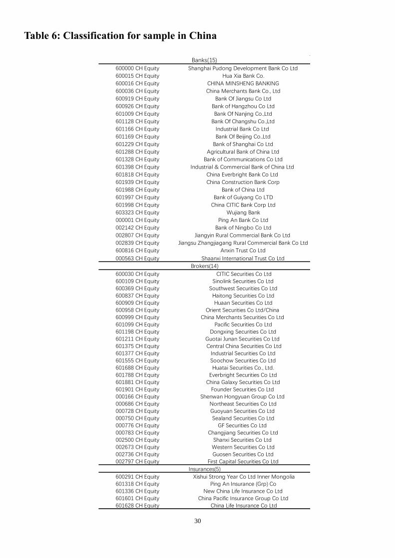
We study a panel of financial institutions in the Taiwan stock market and China stock market from July,

2005 to March, 2017. Their daily log returns, their book value of debt and market value of equity are obtained

from the Bloomberg database. As a proxy for the market's return, we use the Taiwan Stock Exchange Weighted

Index and SSE Composite Index, respectively, in our analysis. Table 5 and Table 6 reports the full list of stock

IDs, tickers and company names by industry groups. SRISK in these two regions are estimated by the same

approach as before.



Figure 4 revels that the aggregate SRISK in China and Taiwan are quite different from US. We find that

the structure of SRISK contribution from different sectors in both China and Taiwan is stable compared with

high mobility among different sectors in U.S.. In Taiwan, financial holding companies dominate the

contribution of SRISK and in China almost all the systemic risk is from banks.

Notice that SRISK in China is rising at a breathtaking pace in the past 10years and there is no clear

evidence of significantly declining in recent years. This finding may correspond to a recent warning to restrain

systemic risk from the Chinese government5.

4 Although the Volatility Laboratory (V-Lab) of the NYU Stern School website provides China’s and Taiwan's SRISK index, it only considers llimited financial

institutions in China and Taiwan. V-Lab is a systemic risk measurement provider for U.S. and global financial firms. It is based at New York University Stern

School of Business under the direction of NYU Stern Professor Robert Engle (see http://vlab.stern.nyu.edu/).

5 “Xi Stresses Reining in Systemic Risks as China's Leaders Gather” according to Bloomberg News： President Xi Jinping said China will continue "seeking progress while

maintaining stability" this year and that better supervision is needed to control financial risk, according to the official Xinhua News Agency.

20

5.3 Compared with other Capital Shortfall Measures

We compared our systemic risk estimations, called SRISK, with other capital shortage measures, which

include systemic expected shortfall (SES) and Engle-SRISK based on the GARCH-DCC model. SES

measures the expected shortage of capital for individual companies in the event of a significant capital shortage

in the system.

The outbreak of the financial crisis will have a long-term and deep impact on the financial system, and

the risk of the financial system will have a very strong negative external effects. From the perspective of

government regulation, by bailing out those companies with the most capital shortages can reduce effectively

the systemic risk. In 2007-2009, the Federal Reserve implemented the Troubled Asset Relief Program (TARP)

to capitalize on capital shortages. Among the sampled financial institution, 40 of them have received the plan.

TARP's capital injection can be seen as a relatively accurate substitute for the company's capital shortage

during the crisis, so we use the Tobit regression model to assess the predictive effect of SRISK on TARP

capital injection.

logTCapitali∗= α0 + β log(1 + (SRISKi)+) + γbi + εi

where ：logTCapitali= {

logTCapitali∗ , logTCapitali

∗> 0

0 , others ,TCapitali

denotes the capital injection of firm i

during crisis, bi denotes some control variables, including sectors（dummy variable）, firm’s total asset,

current volatility of stock, SES, Engle-SRISK based on GARCH-DCC model, and εi is i.i.d. shock.

Table 7 records the results of the Tobit model estimates. When the Tobit model contains only the sector

classification, the log company's total assets and the company's stock price volatility, its interpretation of

21

capital injection TCapitaliis explained as 11.2%. The addition of SRISK makes the pseudo R-square up to

29.1%, and the SRISK coefficient is 0.63 being statistically significant. The pseudo R-square’s contributed

from other capital shortage indicators such as SES and Engle-SRISK are relatively small, respectively, 18.6%

and 20.3%. Comparing all the indicators in the model, it can be seen that SRISK has a more significant

statistical significance than other capital shortages. To sum up, SRISK has an effective support for capital

injection and capital shortages.


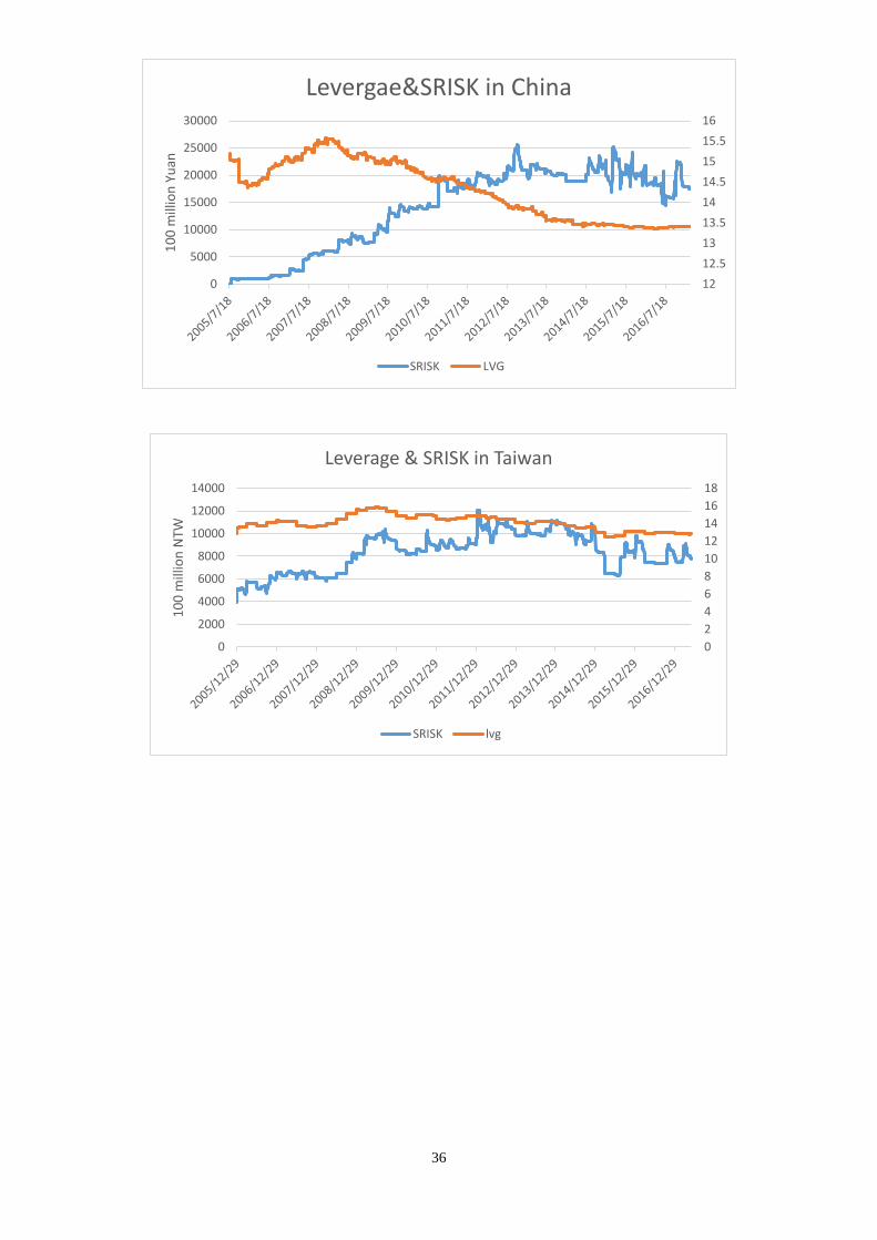
5.4 Leverage and SRISK

Since SRISK can be a good proxy of systemic risk, we are interested in the effect of leverage weighted

by firm’s equity. We can observe a positive correlation between leverage and SRISK in both the U.S. and

Taiwan markets. Their leverages are relatively high throughout the financial crisis. Systemic risk is usually

descending with the deleveraging over the last period of crisis.

It is interesting that leverage of financial institutions in China is quite high before 2011. After financial

crisis, Chinese government are consciously guiding financial institutions in deleveraging, which can be seen

from Figure 6 that leverage declined from 16 to 13.5. From the government’s recent report deleverage will

remain a major driving force to control their systemic risk6.


Section 6: Conclusion

SRISK measures the expected capital shortfall of a financial institution conditional on a prolonged and

severe market decline. We investigate SRISK estimation under dynamic volatility matrix models by proposing

an improved procedure and comparing its estimation performance with major traditional methods. Fourier

transform method to estimate the dynamic volatility matrix and enhanced importance sampling to estimate

SRISK are crucial to provide accurate results.

6 http://www.pbc.gov.cn/english/130721/3401747/index.html

22

We use this methodology to analyze the systemic risk of top financial firms in US, Taiwan and China

between 2005 and 2016. The systemic risk analysis is useful to measure the stability of financial system and

it can provide early signs for the financial crisis. And we obseve that leverage can be an important driving

force to systemic risk in cases of the U.S. , China and Taiwan..

23

References

Acharya, V., Pedersen, L. H., Philippon, T., & Richardson, M. (2017). Measuring systemic risk. The Review

of Financial Studies, 30(1), 2-47.

Acharya, V., Engle, R., & Richardson, M. (2012). Capital shortfall: A new approach to ranking and

regulating systemic risks. The American Economic Review, 102(3), 59-64.

Adrian, T., Brunnermeier, M. K. (2016). CoVaR. The American Economic Review, 106(7), 1705-1741.

Aı Y, Kimmel R. (2007) Maximum likelihood estimation of stochastic volatility models[J]. Journal of

Financial Economics, 83(2): 413-452.

` `

Alessi, Lucia, and Carsten. (2009). Real time early warning indicators for costly asset price boom/bust

cycles: a role for global liquidity. ECB Working Paper No. 1039

Bayazitova, D., Shivdasani, A. (2011). Assessing tarp. The Review of Financial Studies, 25(2), 377-407.

Billio, M., Getmansky, M., Lo, A. W., & Pelizzon, L. (2010). Measuring systemic risk in the finance and

insurance sectors. MIT Sloan School of Management Working Paper;4774-10

Bisias, Dimitrios, et al. (2012). A survey of systemic risk analytics. Annu. Rev. Financ. Econ. 4.1: 255-296.

Financial Stability Board. (2009). Guidance to assess the systemic importance of financial institutions,

markets and instruments: initial considerations. Report to G20 finance ministers and governors

Borio, C., Drehmann, M. (2011). Toward an operational framework for financial stability: “fuzzy”

measurement and its consequences. Central Banking, Analysis, and Economic Policies Book Series, 15, 63-

123

Brownlees, C., Engle, R. F. (2016). SRISK: A conditional capital shortfall measure of systemic risk. The

Review of Financial Studies, 30(1), 48-79.

Caballero, Ricardo J., and Arvind Krishnamurthy. (2009). Global imbalances and financial fragility. No.

w14688. National Bureau of Economic Research

24

De Bandt, Olivier, and Philipp Hartmann. (2000). Systemic Risk: A Survey, European

Central Bank Working Paper No. 35.

Engle, Jondeau, and Rockinger. (2015). Systemic risk in Europe. Review of Finance 19.1: 145-190.

Engle, R. (2002). Dynamic conditional correlation: A simple class of multivariate generalized autoregressive

conditional heteroskedasticity models. Journal of Business & Economic Statistics, 20(3), 339-350.

Fouque, J.-P., Papanicolau, G., Sircar, R.,and Solna, K. (2011). Multiscale Stochastic Volatility for Equity,

Interest Rate, and Credit Derivatives. Cambridge University Press.

Gray, D. F., Merton, R. C., and Bodie, Z. (2007). New framework for measuring and

managing macro financial risk and financial stability. Working Paper 13607, National

Bureau of Economic Research.

Han, C.-H. (2013). Instantaneous Volatility Estimation by Fourier Transform Methods. Hanbook of

Financial Econometrics and Statistics. Editor: C.-F. Lee. Springer.

Han, C. H., Liu, W. H., & Chen, T. Y. (2014). VaR/CVaR estimation under stochastic volatility models.

International Journal of Theoretical and Applied Finance, 17(02), 1450009.

Heston, S. L. (1993). A closed-form solution for options with stochastic volatility with applications to bond

and currency options. The review of financial studies, 6(2), 327-343.

Hull, J. (2008). Options, futures, and other derivatives (7th ed.). Prentice Hall.

Fouque, J. P., & Langsam, J. A. (Eds.). (2013). Handbook on systemic risk. Cambridge University Press.

Junlu M, Xiaoyun F, Yuantao C. (2007). Estimating Bilateral Exposures in the China Interbank Market: Is

There a Systemic Contagion [J]. Economic Research Journal, 1: 005.

Kapadia, Sujitet al. (2012). Liquidity risk, cash flow constraints, and systemic feedbacks. Quantifying

Systemic Risk. University of Chicago Press. 29-61.

Kobayashi S.(2017).Insurance and financial stability: implications of the 2016 IMF Global Financial

Stability Report for regulation and supervision of insurers[J]. Journal of Financial Regulation and

Compliance, 25(1).

Malliavin P, Mancino M. E. (2002). Fourier series method for measurement of multivariate volatilities.

Finance and Stochastics, 6(1): 49-61.

25

Mancino, M. E., Recchioni, M. C., & Sanfelici, S. (2017). Fourier-Malliavin Volatility Estimation: Theory

and Practice (1th ed.) Springer

Malliavin, P. and Mancino, M. E. (2009). A Fourier Transform Method for Nonparametric Estimation of

Multivariate Volatility. The Annals of Statistics, 37, 1983-2010.

Merton. (1973). Theory of rational option pricing. The Bell Journal of economics and management science:

141-183.

Mishkin.(2007). The economics of money, banking, and financial markets. Pearson education,

Petrone, D., & Latora, V. (2016). A hybrid approach to assess systemic risk in financial networks. arXiv

preprint arXiv:1610.00795.

Ross, S. (2015). The recovery theorem. The Journal of Finance, 70(2), 615-648.

Reinhart, et al. (2009). This time is different: Eight centuries of financial folly. princeton university press,

Rosengren, Eric S. (2010). Asset bubbles and systemic risk. The Global Interdependence Center's

Conference on "Financial Interdependence in the World's Post-Crisis Capital Markets", Philadelphia, March

3, 2010

Tankov P. Financial modelling with jump processes[M]. CRC press, 2003.

U.S. Congress. (2010). Dodd-Frank Wall Street reform and consumer protection act, Public Document H.R.

4173.

26

Table 1: Parameters setting

Heston parameters Jacobi

parameters

𝜅𝑚 𝜃𝑚 𝜉𝑚 𝜇𝑚 𝜌𝑚 𝑆𝑚0 𝑣𝑚0 𝛼𝑖 𝑚𝑖

3 0.5 1 0.1 -0.5 2000 0.5 10 0.3

𝜅𝑖 𝜃𝑖 𝜉𝑖 𝜇𝑖 𝜌𝑖 𝑆𝑖0 𝑣𝑚𝑖 𝛽𝑖 𝜌0

5 0.7 2 0.08 -0.6 400 0.7 1 0.3

Table 2: Simulation with Importance Sampling

Constant volatility

Hitting time style crisis

c Prob(CMC) s.e. LRMES Prob(IS) s.e. LRMES V.V.R

-0.2 1.137E-02 3.35E-04 1.161E-01 1.144E-03 9.129E-05 1.109E-01 1.35E+01

-0.3 2.60E-04 5.098E-05 1.388E-01 2.113E-04 2.576E-06 1.623E-01 3.92E+02

-0.4 0 0 0 1.063E-07 1.936E-08 2.126E-01 0.00E+00

-0.5 0 0 0 1.373E-09 3.295E-09 2.63E-01 0.00E+00

V.V.R. stands for variance reduction ratio V. V. R. = (𝑠. 𝑒. (𝐶𝑀𝐶)

𝑠. 𝑒. (𝐼𝑆)⁄ )2

Stochastic volatility

Hitting time style crisis

c Prob(CMC) s.e. LRMES Prob(IS) s.e. LRMES V.V.R

-0.2 2.706E-01 1.405E-03 9.609E-02 2.679E-01 1.041E-03 9.516E-02 1.822E+00

-0.3 1.091E-01 9.858E-04 1.321E-01 1.076E-01 5.668E-04 1.355E-01 3.025E+00

-0.4 1.730E-03 1.314E-04 2.616E-01 1.829E-03 1.968E-05 2.487E-01 4.458E+01

-0.5 6.000E-05 2.449E-05 2.783E-01 3.794E-05 5.165E-07 3.311E-01 2.248E+03

V.V.R. stands for variance reduction ratio V. V. R. = (𝑠. 𝑒. (𝐶𝑀𝐶)

𝑠. 𝑒. (𝐼𝑆)⁄ )2

27

Table 3: Classification for sample in US

BAC Bank of America AET Aetna ETFC E-TradeFinancial ACAS AmericanCapitalBBT BB&T AFL Aflac GS GoldmanSachs AMP AmeripriseFinancialBK Bank of New York Mellon AIG AmericanInternationalGroup LEH LehmanBrothers AMTD TDAmeritradeC Citigroup AIZ Assurant MER MerrillLynch AXP AmericanExpressCBH Commerce Bancorp ALL AllstateCorp MS MorganStanley BEN FranklinResourcesCMA Comerica inc WRB W.R.BerkleyCorp NMX NymexHoldings BLK BlackrockHBAN Huntington Bancshares BRK BerkshireHathaway SCHW SchwabCharles BOT CBOTHoldingsHCBK HUDSON City Bancorp CB ChubbCorp TROW T.RowePrice CBG C.B.RichardEllisGroupJPM JP Morgen Chase CFC CountrywideFinancial CBSS CompassBancsharesKEY Key corp CI CIGNACorp CIT CITGroupMTB M&TBankCorp CINF CincinnatiFinancialCorp CME CMEGroupNCC NationalCityCorp CNA CNAFinancialcorp COF CapitalOneFinancialNTRS NorthernTrust CVH CoventryHealthCare FITB FifthThirdBancorpNYB NewYorkCommunityBancorp FNF FidelityNationalFinancial FNM FannieMaePBCT PeoplesUnitedFinancial GNW GenworthFinancial FRE FreddieMacPNC PNCFinancialServices HIG HartfordFinancialGroup ICE IntercontinentalExchangeRF RegionsFinancial HNT HealthNet JNS JanusCapitalSNV SynovusFinancial HUM Humana MA MastercardSTI SuntrustBanks LNC LincolnNational LM LeggMasonSTT StateStreet MBI MBIA NYX NYSEEuronextUSB USBancorp MET Metlife SEIC SEIInvestmentsCompanyWFC WellsFargo&Co MMC Marsh&McLennan SLM SLMCorpWM WashingtonMutual PFG PrincipalFinancialGroupWU WesternUnion PGR ProgressiveZION Zion PRU PrudentialFinancial

TMK TorchmarkTRV TravelersUNH UnitedhealthGroupUNM UnumGroup

Depositories(25) Insurance(29) Broker-Dealers(8) Others(22)

28

Table 4: SRISK% Ranking

2005Q3 SRISK% 2006Q3 SRISK% 2007Q3 SRISK%

FNM 13.83% FNM 14.13% LEH US Equity 14.70%FRM 12.06% FRM 11.08% FNM 12.35%MS Equity 10.04% LEH US Equity 10.73% FRM 13.11%BSC Equity 8.16% GS US Equity 7.98% WFC US Equity 12.37%LEH US Equity 5.45% MS 6.40% GS US Equity 3.69%PRU Equity 3.59% WFC US Equity 5.17% BSC Equity 3.57%MMC US Equity 3.26% CVH US Equity 3.15% CVH US Equity 2.08%WRB US Equity 2.42% MMC US Equity 2.09% MMC US Equity 1.89%GS 2.26% WRB US Equity 1.59% WRB US Equity 1.18%NCC US Equity 2.13% SEIC US Equity 1.41% SEIC US Equity 0.91%


C US Equity 13.53% BAC 15.72% PRU US Equity 26.60%MER 11.91% C US Equity 13.50% C US Equity 18.34%GS US Equity 8.45% WFC US Equity 10.42% AIG 15.33%LEH US Equity 7.68% JPM Equity 9.82% MMC US Equity 4.01%AIG 3.12% AIG 2.29% WRB US Equity 3.14%MMC US Equity 2.38% CVH US Equity 2.29% STI US Equity 2.52%CVH US Equity 2.14% MMC US Equity 2.10% NCC US Equity 2.07%BSC Equity 2.03% WRB US Equity 1.83% WFC US Equity 1.76%SEIC US Equity 1.98% SEIC US Equity 1.53% GS US Equity 1.41%WRB US Equity 1.50% HNT US Equity 1.17% HNT US Equity 1.29%


MMC US Equity 16.56% MMC US Equity 17.94% MMC US Equity 20.84%CVH US Equity 14.82% CVH US Equity 13.14% CVH US Equity 11.15%SEIC US Equity 12.08% SEIC US Equity 12.37% STI US Equity 10.83%C US Equity 6.58% STI US Equity 8.89% SEIC US Equity 9.87%STI US Equity 5.59% GS US Equity 8.23% HNT US Equity 7.58%NCC US Equity 5.48% WRB US Equity 5.72% GS US Equity 4.84%GS US Equity 4.98% CFC US Equity 4.66% CFC US Equity 4.68%CFC US Equity 3.48% HNT US Equity 4.54% WRB US Equity 4.18%HNT US Equity 2.80% FITB US Equity 2.76% FITB US Equity 3.27%CINF US Equity 0.79% BBT US Equity 0.70% BBT US Equity 0.37%


MMC US Equity 31.18% MMC US Equity 27.48% MMC US Equity 28.81%CFC US Equity 19.39% HNT US Equity 12.57% HNT US Equity 15.63%CVH US Equity 15.58% HCBK US Equity 9.21% CFC US Equity 12.91%HNT US Equity 11.42% CFC US Equity 8.77% CVH US Equity 11.30%FITB US Equity 5.83% FITB US Equity 7.79% FITB US Equity 8.68%WRB US Equity 3.50% CVH US Equity 7.02% HCBK US Equity 3.89%SEIC US Equity 2.60% WRB US Equity 2.92% BBT US Equity 3.51%HCBK US Equity 2.44% BBT US Equity 1.94% WRB US Equity 0.48%BBT US Equity 1.06% SEIC US Equity 0.00% WFC US Equity 0.00%STI US Equity 0.00% STI US Equity 0.00% PRU US Equity 0.00%

29

Table 5: Classification for sample in Taiwan

30

Table 6: Classification for sample in China

600000 CH Equity Shanghai Pudong Development Bank Co Ltd

600015 CH Equity Hua Xia Bank Co.

600016 CH Equity CHINA MINSHENG BANKING

600036 CH Equity China Merchants Bank Co., Ltd

600919 CH Equity Bank Of Jiangsu Co Ltd

600926 CH Equity Bank of Hangzhou Co Ltd

601009 CH Equity Bank Of Nanjing Co.,Ltd

601128 CH Equity Bank Of Changshu Co.,Ltd

601166 CH Equity Industrial Bank Co Ltd

601169 CH Equity Bank Of Beijing Co.,Ltd

601229 CH Equity Bank of Shanghai Co Ltd

601288 CH Equity Agricultural Bank of China Ltd

601328 CH Equity Bank of Communications Co Ltd

601398 CH Equity Industrial & Commercial Bank of China Ltd

601818 CH Equity China Everbright Bank Co Ltd

601939 CH Equity China Construction Bank Corp

601988 CH Equity Bank of China Ltd

601997 CH Equity Bank of Guiyang Co LTD

601998 CH Equity China CITIC Bank Corp Ltd

603323 CH Equity Wujiang Bank

000001 CH Equity Ping An Bank Co Ltd

002142 CH Equity Bank of Ningbo Co Ltd

002807 CH Equity Jiangyin Rural Commercial Bank Co Ltd

002839 CH Equity Jiangsu Zhangjiagang Rural Commercial Bank Co Ltd

600816 CH Equity Anxin Trust Co Ltd

000563 CH Equity Shaanxi International Trust Co Ltd

600030 CH Equity CITIC Securities Co Ltd600109 CH Equity Sinolink Securities Co Ltd 600369 CH Equity Southwest Securities Co Ltd600837 CH Equity Haitong Securities Co Ltd600909 CH Equity Huaan Securities Co Ltd600958 CH Equity Orient Securities Co Ltd/China 600999 CH Equity China Merchants Securities Co Ltd 601099 CH Equity Pacific Securities Co Ltd601198 CH Equity Dongxing Securities Co Ltd601211 CH Equity Guotai Junan Securities Co Ltd 601375 CH Equity Central China Securities Co Ltd601377 CH Equity Industrial Securities Co Ltd601555 CH Equity Soochow Securities Co Ltd601688 CH Equity Huatai Securities Co., Ltd.601788 CH Equity Everbright Securities Co Ltd601881 CH Equity China Galaxy Securities Co Ltd601901 CH Equity Founder Securities Co Ltd 000166 CH Equity Shenwan Hongyuan Group Co Ltd 000686 CH Equity Northeast Securities Co Ltd000728 CH Equity Guoyuan Securities Co Ltd 000750 CH Equity Sealand Securities Co Ltd000776 CH Equity GF Securities Co Ltd 000783 CH Equity Changjiang Securities Co Ltd002500 CH Equity Shanxi Securities Co Ltd 002673 CH Equity Western Securities Co Ltd002736 CH Equity Guosen Securities Co Ltd002797 CH Equity First Capital Securities Co Ltd

600291 CH Equity Xishui Strong Year Co Ltd Inner Mongolia601318 CH Equity Ping An Insurance (Grp) Co601336 CH Equity New China Life Insurance Co Ltd601601 CH Equity China Pacific Insurance Group Co Ltd601628 CH Equity China Life Insurance Co Ltd

Banks(15)

Brokers(14)

Insurances(5)

31

Table 7：TARP Capital Injection

Const 8.10 *** 1.19 -2.92 -1.26 5.84

Broker -10.69 *** -8.54 *** -11.9 *** -10.3 *** -7.84 ***

Insurance -4.03 -1.57 -2.75 -1.97 -1.72

Others -12.71 *** -9.03 *** -11.5 *** -10.5 *** -8.92 ***

Asset 1.60 *** 1.58 *** 1.83 *** 1.78 *** 1.14 **

Volatility -0.16 -0.31 *** -0.21 ** -0.19 ** -0.34 ***

SES 6.21 *** 2.492.167

Engle_SRISK 0.51 *** 0.4 *0.228

SRISK 0.63 *** 0.46 **

pseudo R2

0.12

0.38

2.32 2.241

2.458

1.542

2.82

3.12

2.829

4.125

0.699

3.144

4.362

2.399

4.472

0.824

3.895

5.342

2.192

4.792

0.087

2.691

0.433

0.109

31.5%29.1%20.3%18.6%11.2%0.228

5.3

1.867

2.369

2.005

0.586

0.112

0.207

0.192

0.103

32

Figure 1: Simulation of market index & firm’s volatility

Figure 2: Simulation of market index & firm’s correlation

33

Figure 3: Time series changes of all company average Heston parameter

Figure 4: Aggregate SRISK with Importance Sampling by Sector in US

0

500

1000

1500

2000

2500

0

100000

200000

300000

400000

500000

600000

700000

Aggregate US_SRISK by Sector

Deposites Brokers Insurance Others S&P500

34

Figure 5： SRISK of Goldman Sachs, Citi and Lehman Brothers

200

2200

4200

6200

8200

10200

12200

14200

10

0 m

illio

n N

TW

Aggregate Taiwan_SRISK by Sector

FHC Banks Insurance

0

5000

10000

15000

20000

25000

30000

10

0 m

illio

n y

uan

Aggregate Mainland China_SRISK by Sector

banking broker insurance

0

20000

40000

60000

80000

100000

1/3/06 1/3/07 1/3/08 1/3/09 1/3/10 1/3/11 1/3/12 1/3/13 1/3/14 1/3/15 1/3/16

GS_SRISK

35

Figure 6： Leverage in SRISK

0

100000

200000

300000

1/3/06 1/3/07 1/3/08 1/3/09 1/3/10 1/3/11 1/3/12 1/3/13 1/3/14 1/3/15 1/3/16

Citi_SRISK

020000400006000080000

LEH_SRISK

0

2

4

6

8

10

12

14

16

0

100000

200000

300000

400000

500000

600000

700000

miil

ion

Leverage & SRISK in US

SRISK LVG

36

12

12.5

13

13.5

14

14.5

15

15.5

16

0

5000

10000

15000

20000

25000

30000

10

0 m

illio

n Y

uan

Levergae&SRISK in China

SRISK LVG

0

2

4

6

8

10

12

14

16

18

0

2000

4000

6000

8000

10000

12000

14000

10

0 m

illio

n N

TW

Leverage & SRISK in Taiwan

SRISK lvg

systemic risk estimation under dynamic volatility matrix

Documents