System software

System software (or systems software) is computer software designed to operate

and control the computer hardware and to provide a platform for running

application software. System software includes the following:

The operating system, allows the parts of a computer to work together by

performing tasks like transferring data between memory and disks or rendering

output onto a display device. It also provides a platform to run high-level system

software and application software.

Utility software helps to analyze, configure, optimize and maintain the computer.

Device drivers such as computer BIOS and device firmware provide basic

functionality to operate and control the hardware connected to or built into the

computer.

system software also includes software development tools (like

a compiler, linker or debugger).

Simplified Instructional Computer (SIC)

SIC is a hypothetical computer that includes the hardware features most often

found on real machines .SIC comes in two versions

•The standard model

•An XE version

“extra equipments”, “extra expensive”

The two versions have been designed to be upward compatible

SIC/XE Machine Architecture:-

Memory:

•8-bit bytes

•3 consecutive bytes form a word (24-bits)

•Addresses are byte addresses

•Words are addressed by location of their lowest numbered byte

•Memory size = 32, 768 (215 bytes)

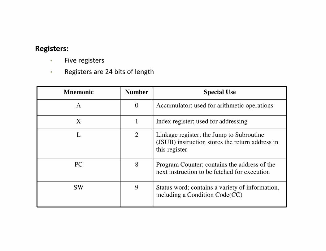
Registers:

• Five registers

• Registers are 24 bits of length

Mnemonic Number Special Use

A 0 Accumulator; used for arithmetic operations

X 1 Index register; used for addressing

L 2 Linkage register; the Jump to Subroutine (JSUB) instruction stores the return address in this register

PC 8 Program Counter; contains the address of the next instruction to be fetched for execution

SW 9 Status word; contains a variety of information, including a Condition Code(CC)

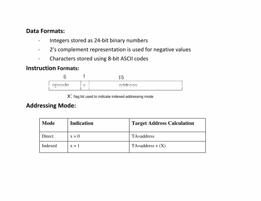
Data Formats:

• Integers stored as 24-bit binary numbers

• 2’s complement representation is used for negative values

• Characters stored using 8-bit ASCII codes

Instruction Formats:

x: flag bit used to indicate indexed-addressing mode

Addressing Mode:

Mode Indication Target Address Calculation

Direct x = 0 TA=address

Indexed x = 1 TA=address + (X)

Instruction Set:

•Load/store registers: LDA, LDX, STA, STX

•Integer arithmetic: ADD, SUB, MUL, DIV

•All involve register A and a word in memory, result stored in register A

•COMP

•Compare value in register A with a word in memory

•Set a condition code CC (<, =, or >)

•Conditional jump instructions

•JLT, JEQ, JGT: test CC and jump

•Subroutine linkage

•JSUB, RSUB: return address in register L

•Input and output

•Performed by transferring 1 byte at a time to or from the rightmost 8

bits of register A

•Each device is assigned a unique 8-bit code, as an operand of I/O

instructions

•Test Device (TD): < (ready), = (not ready)

•Read Data (RD), Write Data (WD)

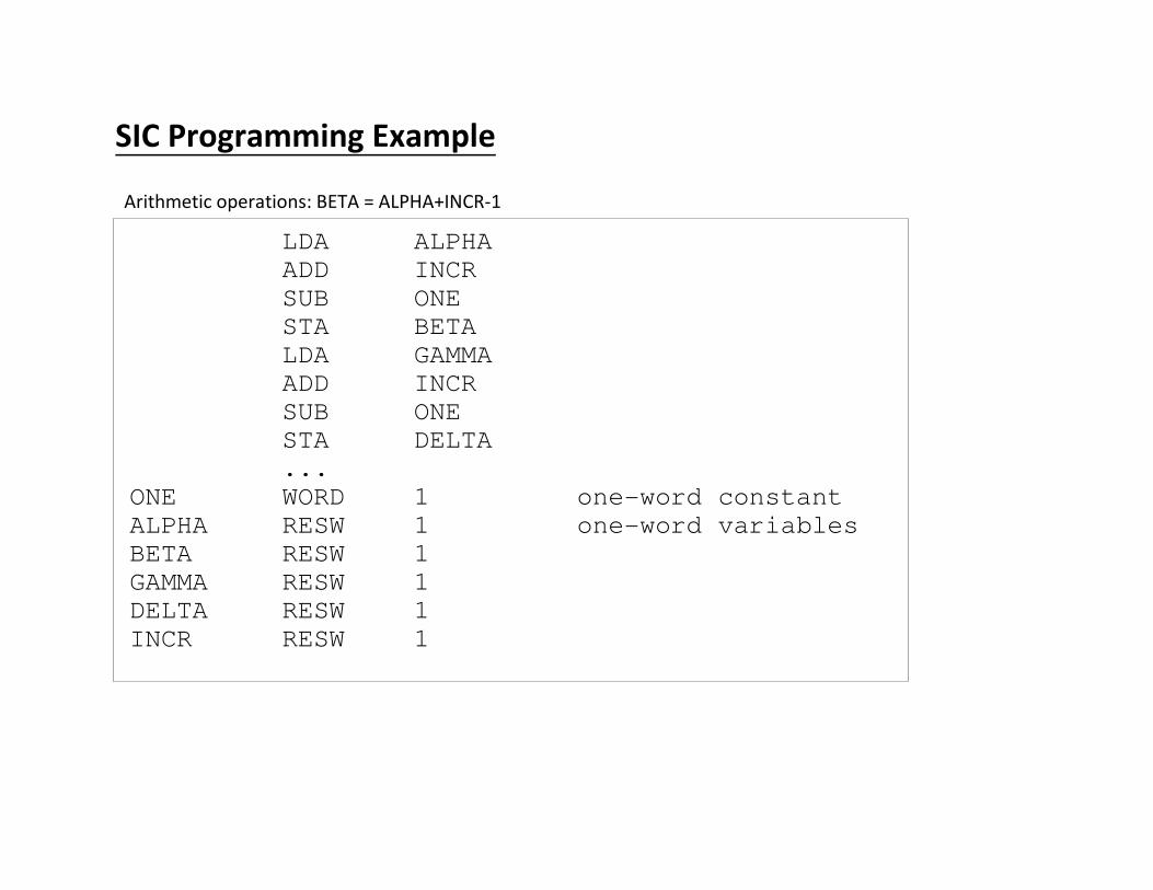
SIC Programming Example

LDA ALPHA

ADD INCR

SUB ONE

STA BETA

LDA GAMMA

ADD INCR

SUB ONE

STA DELTA

...

ONE WORD 1 one-word constant

ALPHA RESW 1 one-word variables

BETA RESW 1

GAMMA RESW 1

DELTA RESW 1

INCR RESW 1

Arithmetic operations: BETA = ALPHA+INCR-1

Looping and indexing: copy one string to another

LDX ZERO initialize index register to 0MOVECH LDCH STR1,X load char from STR1 to reg A

STCH STR2,X

TIX FOUR add 1 to index, compare to 4JLT MOVECH loop if “less than”.

.

.

STR1 BYTE C’TEST’

STR2 RESB 4

ZERO WORD 0

FOUR WORD 4

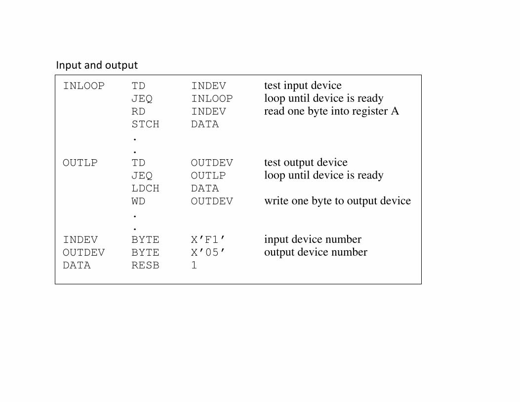
Input and output

INLOOP TD INDEV test input deviceJEQ INLOOP loop until device is readyRD INDEV read one byte into register ASTCH DATA

.

.

OUTLP TD OUTDEV test output deviceJEQ OUTLP loop until device is readyLDCH DATA

WD OUTDEV write one byte to output device.

.

INDEV BYTE X’F1’ input device numberOUTDEV BYTE X’05’ output device numberDATA RESB 1

SIC/XE Machine Architecture

Memory:

• Maximum memory available on a SIC/XE system is 1 megabyte (220 bytes)

• An address (20 bits) cannot be fitted into a 15-bit field as in SIC Standard

• Must change instruction formats and addressing modes

Registers:

Additional registers are provided by SIC/XE

Mnemonic Number Comment

B 3 Base Register (for addressing)

S 4 General Purpose Register

T 5 General Purpose Register

F 6 Floating point Accumalator (48-bits)

1 11 36

s exponent fraction

f*2(e-1024)

There is a 48-bit floating-point data type

• fraction is a value between 0 and 1

• exponent is an unsigned binary number between 0 and 2047

• zero is represented as all 0

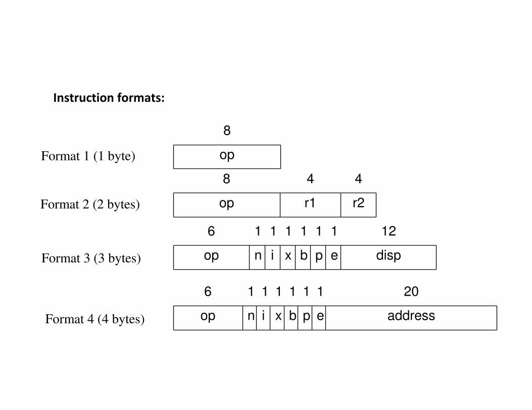
Instruction formats:

8

op

8 4 4

op r1 r2

Format 1 (1 byte)

Format 2 (2 bytes)

6 1 1 1 1 1 1 12

op n i x b p e dispFormat 3 (3 bytes)

6 1 1 1 1 1 1 20

op n i x b p e addressFormat 4 (4 bytes)

n i x b p e

opcode 1 0 disp

Addressing Mode:

Base Relative Addressing Mode

Program-Counter Relative Addressing Mode

b=1, p=0, TA=(B)+disp (0≤disp ≤4095)

n i x b p e

opcode 0 1 disp

b=0, p=1, TA=(PC)+disp (-2048≤disp ≤2047)

n i x b p e

opcode 0 0 disp

Direct Addressing Mode:

b=0, p=0, TA=disp (0≤disp ≤4095)

n i x b p e

opcode 1 0 0 disp

b=0, p=0, TA=(X)+disp

(with index addressing mode)

n i x b p e

opcode 0 1 0 disp

Immediate Addressing Mode:

Indirect Addressing Mode:

n=0, i=1, x=0, operand=disp

n i x b p e

opcode 1 0 0 disp

n=1, i=0, x=0, TA=(disp)

n i x b p e

opcode 0 0 disp

Simple Addressing Mode:

i=0, n=0, TA=bpe+disp (SIC standard)

opcode+n+i = SIC standard opcode (8-bit)

n i x b p e

opcode 1 1 disp

i=1, n=1, TA=disp (SIC/XE standard)

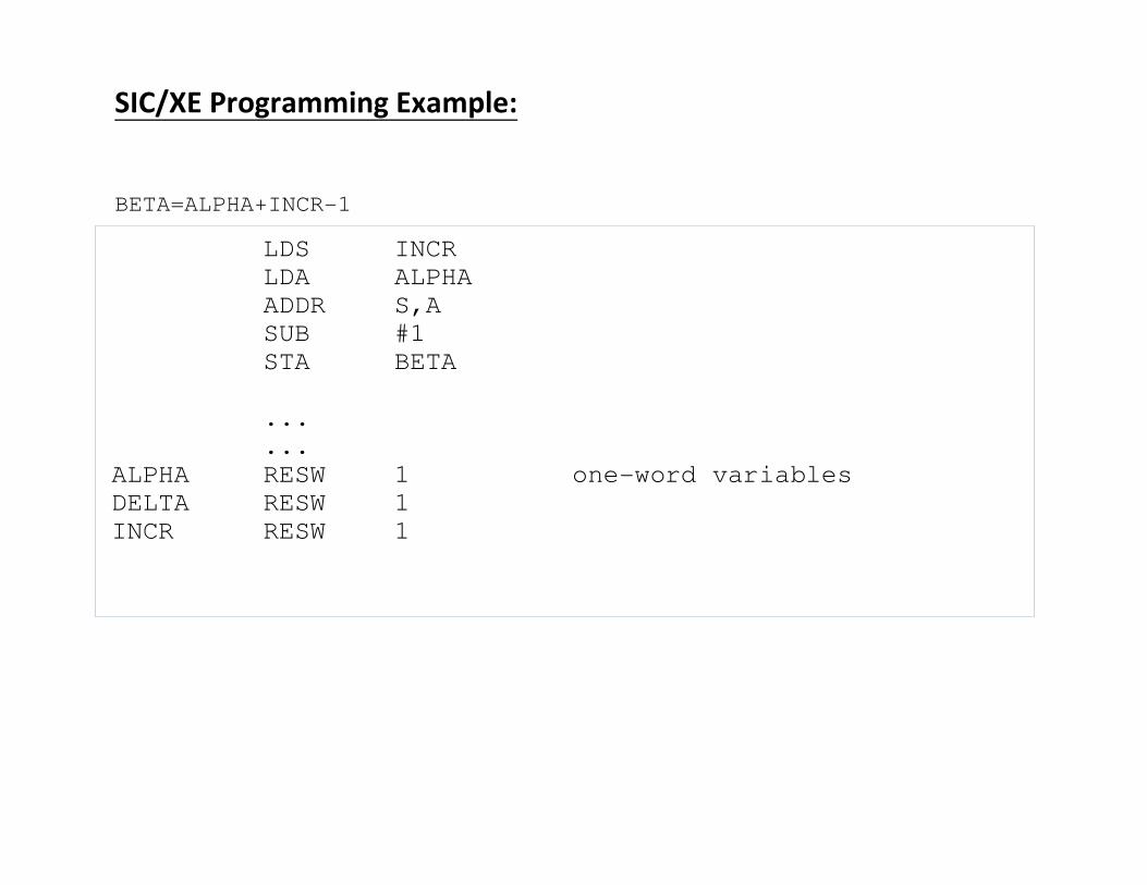
SIC/XE Programming Example:

BETA=ALPHA+INCR-1

LDS INCR

LDA ALPHA

ADDR S,A

SUB #1

STA BETA

...

...

ALPHA RESW 1 one-word variables

DELTA RESW 1

INCR RESW 1

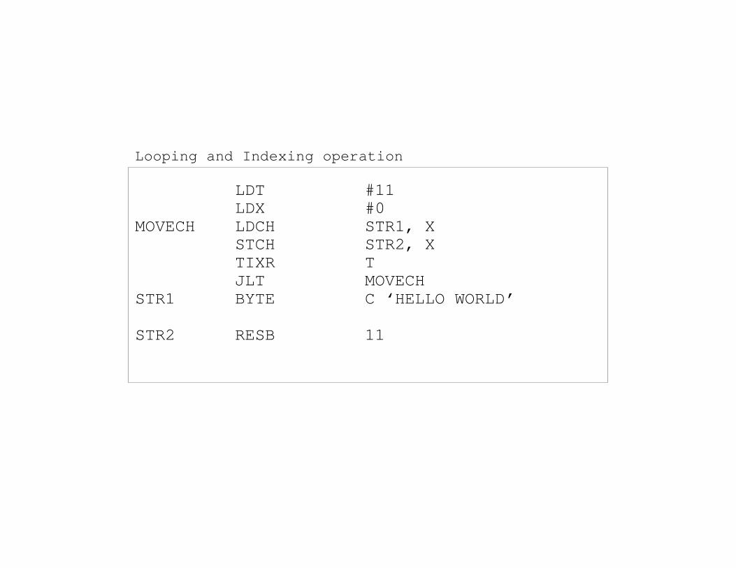
Looping and Indexing operation

LDT #11

LDX #0

MOVECH LDCH STR1, X

STCH STR2, X

TIXR T

JLT MOVECH

STR1 BYTE C ‘HELLO WORLD’

STR2 RESB 11

Assemblers

An assembler is a program that accepts assembly program as

input and produces its machine language equivalent along with

information for the loader.

AssemblerAssembly language

Program

Machine language and

other information for the

loader

Assembler Directives

Assembler directives are pseudo instructions They will not be translated into machine instructions . They only provide instruction/direction/information to the assembler.

Basic assembler directives :

START Specify name and starting address for the program

END Indicate the end of the source program, and

BYTE Generate character or hexadecimal constant, occupying as many

bytes as needed to represent the constant.

WORD Generate one-word integer constant

RESB Reserve the indicated number of bytes for a data area

RESW Reserve the indicated number of words for a data area

General design procedure

We have to follow six steps

1.Specify the problem

2.Specify data structure

3.Define format of data structure

4.Specify algorithm

5.Look for modularity

6.Repeat 1 to 5 on modules

Statement of problem

BETA = ALPHA+INCR-1

Sum Start 0

LDA ALPHA

ADD INCR

SUB ONE

STA BETA

...

ONE WORD 1

ALPHA RESW 1

BETA RESW 1

INCR RESW 1

End

00 0 ?

Data structure

1. A table, the Machine operation table(MOT),that indicates for each instruction (a)symbolic

mnemonic (b)length (c)binary machine opcode and (d)format.

2. A table, the Pseudo-operation table(POT),that indicates for each pseudo-op the symbolic

mnemonic and the action to be taken.

3. A table, the Symbol table (ST) that is used to store each literal encountered and its

corresponding value.

4. A table, the Literal table that is used to store each literal encountered and its corresponding

assigned location.

Format for data bases

1. Machine-Operation table

Instruction length Instruction format

01=2byte 00=First format

10=3byte 01=Second format

11=4byte

Mnemonic

s op-code

Binary op-

code

Instruction

length

Instruction

format

……..

“LDA” 00 10 00 ……..

“ADDR” 90 10 01 ……..

…….. …….. …….. …….. ……..

2. Pseudo-op Table

3. Symbol Table

Pseudo-op Address of routine to process pseudo-op

“START” P1DROP

“END” P1END

…… ……….

Symbol Value Length Relocation

“ALPHA” 000 03 “R”

“INCR” 003 03 “R”

……… …….. …….. …….

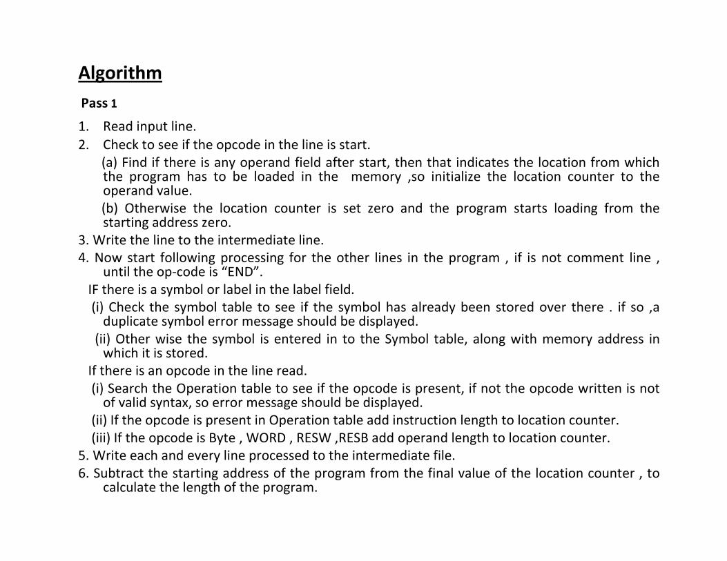
Algorithm

Pass 1

1. Read input line.

2. Check to see if the opcode in the line is start.

(a) Find if there is any operand field after start, then that indicates the location from which the program has to be loaded in the memory ,so initialize the location counter to the operand value.

(b) Otherwise the location counter is set zero and the program starts loading from the starting address zero.

3. Write the line to the intermediate line.

4. Now start following processing for the other lines in the program , if is not comment line , until the op-code is “END”.

IF there is a symbol or label in the label field.

(i) Check the symbol table to see if the symbol has already been stored over there . if so ,a duplicate symbol error message should be displayed.

(ii) Other wise the symbol is entered in to the Symbol table, along with memory address in which it is stored.

If there is an opcode in the line read.

(i) Search the Operation table to see if the opcode is present, if not the opcode written is not of valid syntax, so error message should be displayed.

(ii) If the opcode is present in Operation table add instruction length to location counter.

(iii) If the opcode is Byte , WORD , RESW ,RESB add operand length to location counter.

5. Write each and every line processed to the intermediate file.

6. Subtract the starting address of the program from the final value of the location counter , to calculate the length of the program.

Pass 2

1.Read the first line from the intermediate file.

2.IF so then write the header record to the object program.

3. Start the following processing for the other lines in the intermediate file it is not a comment line until an “END” statement is reached.

(i) Start writing the text record to the output file. If symbol is present in the operand field of the instruction, assemble opcode of the instruction from the Operation table ,with the address of the symbol from the symbol table.

(ii)If the symbol is present in the operand field, and if does not occupy any place in the symbol table then undefined error message should be displayed.

(iii)If there is no symbol in the operand field ,then the operand address is assigned as zero, and it is assembled with the object code of the instruction.

(iv)If the opcode is BYTE, WORD, RESB etc convert the constants to the object code

4.When all the text records have been written to the assembly listing write the END record.

Two Pass Assembler

Pass 1 Pass 2 Intermediate

fileObject

codes

Source

program

OPTAB SYMTAB SYMTAB

Object Program

• HeaderCol. 1 H

Col. 2~7 Program name

Col. 8~13 Starting address (hex)

Col. 14-19 Length of object program in bytes (hex)

• TextCol.1 T

Col.2~7 Starting address in this record (hex)

Col. 8~9 Length of object code in this record in bytes (hex)

Col. 10~69 Object code (69-10+1)/6=10 instructions

• EndCol.1 E

Col.2~7 Address of first executable instruction (hex)

(END program_name)

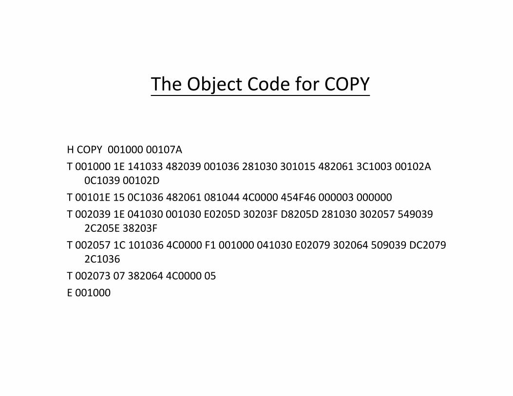
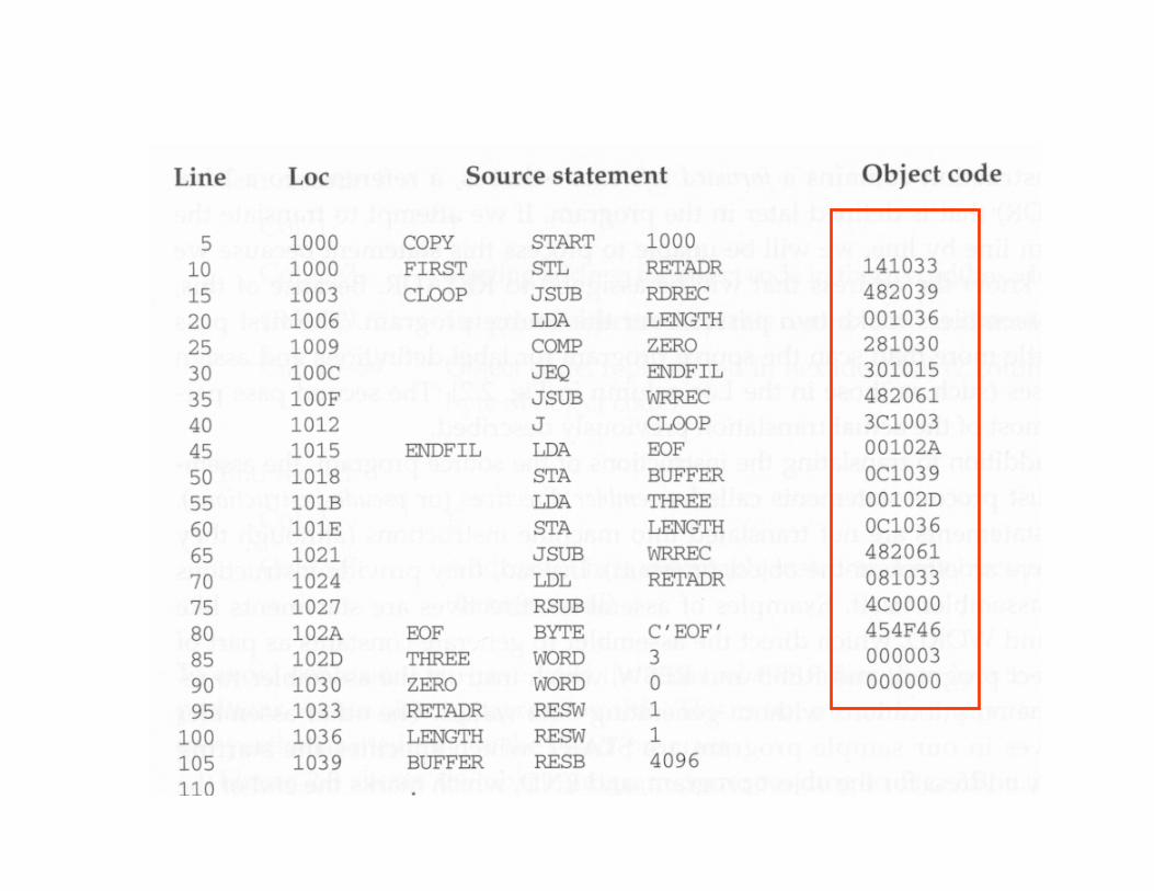
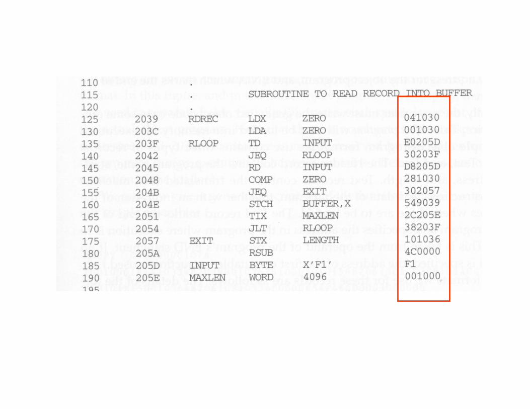
The Object Code for COPY

H COPY 001000 00107A

T 001000 1E 141033 482039 001036 281030 301015 482061 3C1003 00102A

0C1039 00102D

T 00101E 15 0C1036 482061 081044 4C0000 454F46 000003 000000

T 002039 1E 041030 001030 E0205D 30203F D8205D 281030 302057 549039

2C205E 38203F

T 002057 1C 101036 4C0000 F1 001000 041030 E02079 302064 509039 DC2079

2C1036

T 002073 07 382064 4C0000 05

E 001000

Assembler Design

Machine Dependent Assembler Features

• instruction formats and addressing modes

• program relocation

Machine Independent Assembler Features

• literals

• symbol-defining statements

• expressions

• program blocks

• control sections and program linking

Instruction Format and Addressing Mode

SIC/XE

• PC-relative or Base-relative addressing: op m

• Indirect addressing: op @m

• Immediate addressing: op #c

• Extended format: +op m

• Index addressing: op m,x

• register-to-register instructions

• larger memory -> multi-programming (program allocation)

Translation

Register translation

• register name (A, X, L, B, S, T, F, PC, SW) and their values

(0,1, 2, 3, 4, 5, 6, 8, 9)

• preloaded in SYMTAB

Address translation

• Most register-memory instructions use program counter relative or base

relative addressing

• Format 3: 12-bit address field

• base-relative: 0~4095

• pc-relative: -2048~2047

• Format 4: 20-bit address field

Chap 2

PC-Relative Addressing Modes

100000 FIRST STL RETADR17202D

(14)16 1 1 0 0 1 0 (02D) 16

• displacement= RETADR - PC = 30-3 = 2D

400017 J CLOOP 3F2FEC

(3C)16 1 1 0 0 1 0 (FEC) 16

• displacement= CLOOP-PC= 6 - 1A= -14= FEC

op(6) n I x b p e disp(12)

op(6) n I x b p e disp(12)

Base-Relative Addressing Modes

base register is under the control of the programmer

12 LDB #LENGTH

13 BASE LENGTH

160 104E STCH BUFFER, X 57C003

( 54 )16 1 1 1 1 0 0 ( 003 ) 16

(54) 1 1 1 0 1 0 0036-1051= -101B16

• displacement= BUFFER - B = 0036 - 0033 = 3NOBASE is used to inform the assembler that the contents of the base register no

longer be relied upon for addressing.

op(6) n I x b p e disp(12)

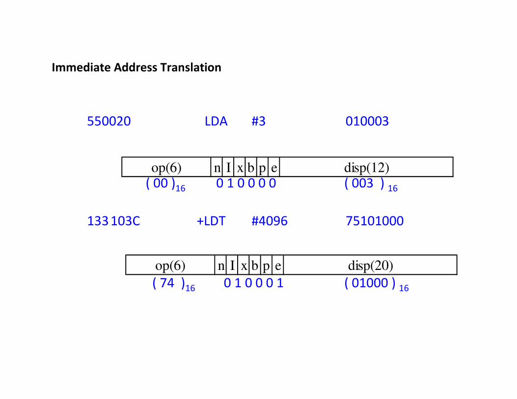
Immediate Address Translation

550020 LDA #3 010003

( 00 )16 0 1 0 0 0 0 ( 003 ) 16

133 103C +LDT #4096 75101000

( 74 )16 0 1 0 0 0 1 ( 01000 ) 16

op(6) n I x b p e disp(12)

op(6) n I x b p e disp(20)

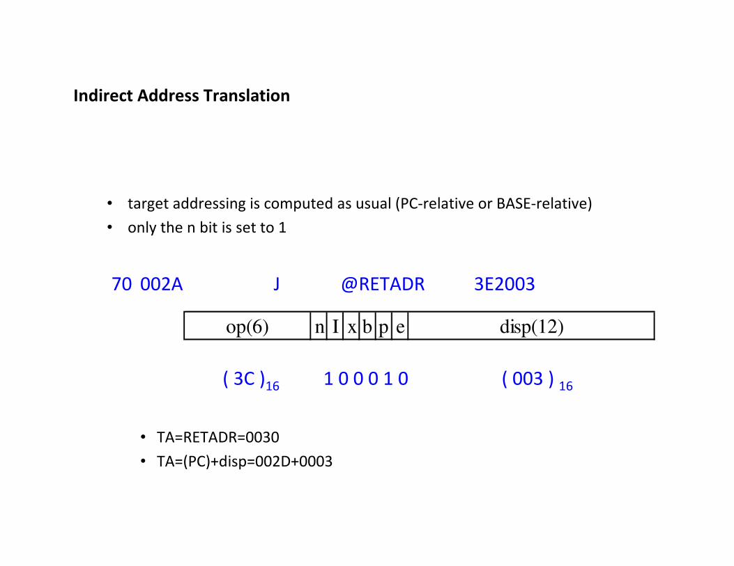
Indirect Address Translation

• target addressing is computed as usual (PC-relative or BASE-relative)

• only the n bit is set to 1

70 002A J @RETADR 3E2003

( 3C )16 1 0 0 0 1 0 ( 003 ) 16

• TA=RETADR=0030

• TA=(PC)+disp=002D+0003

op(6) n I x b p e disp(12)

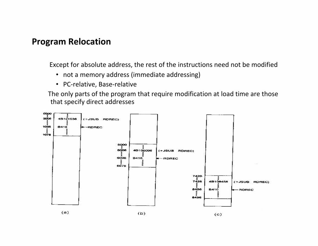
Program Relocation

Except for absolute address, the rest of the instructions need not be modified

• not a memory address (immediate addressing)

• PC-relative, Base-relative

The only parts of the program that require modification at load time are those that specify direct addresses

Modification record

Col 1 M

Col 2-7 Starting location of the address field to be

modified, relative to the beginning of the program

Col 8-9 length of the address field to be modified, in half-

bytes

Literals

• Let programmers to be able to write the value of a constant operand as a part of the instruction that uses it.

• This avoids having to define the constant elsewhere in the program and make up a label for it.

001A ENDFIL LDA =C’EOF’ 032010

93 LTORG

002D * =C’EOF’ 454F46

1062 WLOOP TD =X’05’ E32011

Literals vs. Immediate Operands

• Immediate Operands

The operand value is assembled as part of the machine instruction

e.g. 55 0020 LDA #3 010003

• Literals

The assembler generates the specified value as a constant at some other

memory location

e.g. 45 001A ENDFIL LDA =C’EOF’ 032010

Literal - Implementation

• LITTAB

literal name, the operand value and length, the address assigned to the

operand

• Pass 1– build LITTAB with literal name, operand value and length, leaving the

address unassigned

– when LTORG statement is encountered, assign an address to each literal not yet assigned an address

• Pass 2– search LITTAB for each literal operand encountered

– generate data values using BYTE or WORD statements

– generate modification record for literals that represent an address in the program

Symbol-Defining Statements

• Labels on instructions or data areas

– the value of such a label is the address assigned to the statement

• Defining symbols

– symbol EQU value

– value can be: constant ,other symbol ,expression

– making the source program easier to understand

– no forward reference

Ex

MAXLEN EQU 4096

+LDT #MAXLEN

Expressions

• Expressions can be classified as absolute expressions or relative expressions

– MAXLEN EQU BUFEND-BUFFER

– BUFEND and BUFFER both are relative terms, representing addresses within

the program

– However the expression BUFEND-BUFFER represents an absolute value

• When relative terms are paired with opposite signs, the dependency on the

program starting address is canceled out; the result is an absolute value

SYMTAB

• None of the relative terms may enter into a multiplication or division operation

• Errors:

– BUFEND+BUFFER

– 100-BUFFER

– 3*BUFFER

• The type of an expression

– keep track of the types of all symbols defined in the program

Symbol Type Value

RETADR R 30

BUFFER R 36

BUFEND R 1036

MAXLEN A 1000

Program Blocks

– refer to segments of code that are rearranged within a single object program unit

– USE [blockname]

– Default block

– Each program block may actually contain several separate segments of the source program

Program Blocks - Implementation

Pass 1

– each program block has a separate location counter

– each label is assigned an address that is relative to the start of the block that

contains it

– at the end of Pass 1, the latest value of the location counter for each block

indicates the length of that block

– the assembler can then assign to each block a starting address in the object

program

Pass 2

– The address of each symbol can be computed by adding the assigned block starting

address and the relative address of the symbol to that block

• Each source line is given a relative address assigned and a block number

• For absolute symbol, there is no block number

– line 107

• Example

– 20 0006 0 LDA LENGTH 032060

– LENGTH=(Block 1)+0003= 0066+0003= 0069

– LOCCTR=(Block 0)+0009= 0009

Chap 2

Block name Block number Address Length

(default) 0 0000 0066

CDATA 1 0066 000B

CBLKS 2 0071 1000

Program Readability

• Program readability

– No extended format instructions on lines 15, 35, 65

– No needs for base relative addressing (line 13, 14)

– LTORG is used to make sure the literals are placed ahead of any large data

areas (line 253)

• Object code

– It is not necessary to physically rearrange the generated code in the object

program

Control Sections and Program Linking

• Control Sections

– are most often used for subroutines or other logical subdivisions of a

program

– the programmer can assemble, load, and manipulate each of these

control sections separately

– instruction in one control section may need to refer to instructions or data

located in another section

– because of this, there should be some means for linking control sections

together

External Definition and References

• External definition

– EXTDEF name [, name]

– EXTDEF names symbols that are defined in this control section and may be used

by other sections

• External reference

– EXTREF name [,name]

– EXTREF names symbols that are used in this control section and are defined

elsewhere

• Example

– 15 0003 CLOOP +JSUB RDREC 4B100000

– 160 0017 +STCH BUFFER,X 57900000

– 190 0028 MAXLEN WORD BUFEND-BUFFER 000000

Implementation

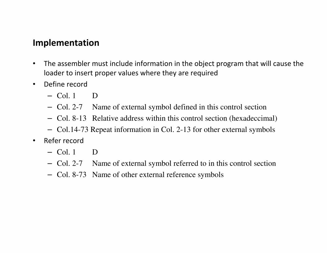
• The assembler must include information in the object program that will cause the

loader to insert proper values where they are required

• Define record

– Col. 1 D

– Col. 2-7 Name of external symbol defined in this control section

– Col. 8-13 Relative address within this control section (hexadeccimal)

– Col.14-73 Repeat information in Col. 2-13 for other external symbols

• Refer record

– Col. 1 D

– Col. 2-7 Name of external symbol referred to in this control section

– Col. 8-73 Name of other external reference symbols

Modification Record

• Modification record

– Col. 1 M

– Col. 2-7 Starting address of the field to be modified (hexiadecimal)

– Col. 8-9 Length of the field to be modified, in half-bytes (hexadeccimal)

– Col.11-16 External symbol whose value is to be added to or subtracted from the indicated field

– Note: control section name is automatically an external symbol, i.e. it is available for use in Modification records.

• Example

– Figure 2.17

– M00000405+RDREC

– M00000705+COPY

External References in Expression

• Earlier definitions

– required all of the relative terms be paired in an expression (an

absolute expression), or that all except one be paired (a relative

expression)

• New restriction

– Both terms in each pair must be relative within the same control

section

– Ex: BUFEND-BUFFER

– Ex: RDREC-COPY

• In general, the assembler cannot determine whether or not the

expression is legal at assembly time. This work will be handled by a

linking loader.

One-Pass Assemblers

• Main problem

– forward references

• data items

• labels on instructions

• Solution

– data items: require all such areas be defined before they are referenced

– labels on instructions: no good solution

• Two types of one-pass assembler

– load-and-go

• produces object code directly in memory for immediate execution

– the other

• produces usual kind of object code for later execution

Load-and-go Assembler

• Characteristics

– Useful for program development and testing

– Avoids the overhead of writing the object program out and reading it back

– Both one-pass and two-pass assemblers can be designed as load-and-go.

– However one-pass also avoids the over head of an additional pass over

the source program

– For a load-and-go assembler, the actual address must be known at

assembly time, we can use an absolute program

• For any symbol that has not yet been defined

1. omit the address translation

2. insert the symbol into SYMTAB, and mark this symbol undefined

3. the address that refers to the undefined symbol is added to a list of forward references associated with the symbol table entry

4. when the definition for a symbol is encountered, the proper address for the symbol is then inserted into any instructions previous generated according to the forward reference list

• At the end of the program

– any SYMTAB entries that are still marked with * indicate undefined symbols

– search SYMTAB for the symbol named in the END statement and jumpto this location to begin execution

• The actual starting address must be specified at assembly time

Producing Object Code

• When external working-storage devices are not available or too slow (for the

intermediate file between the two passes

• Solution:

– When definition of a symbol is encountered, the assembler must generate

another Tex record with the correct operand address

– The loader is used to complete forward references that could not be handled

by the assembler

– The object program records must be kept in their original order when they

are presented to the loader

Loader and Linker

A Loader should perform following three functions-

1. Loading: loading an object program into memory for execution.

2. Relocation: modify the object program so that it can be loaded at an address from the location originally specified.

3. Linking: combines two or more separate object programs and supplies the information needed to allow references between them.

A loader is a system program that performs the loading function. Many loaders also support relocation and linking. Some systems have a linker to perform the linking and a separate loader to handle relocation and loading.

Absolute Loader

1. An object program is loaded at the address specified on the START directive.

2. No relocation or linking is needed

3. Thus is very simple

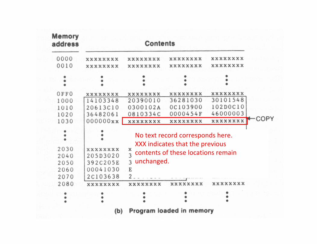
No text record corresponds here.

XXX indicates that the previous

contents of these locations remain

unchanged.

Absolute Loader Implementation

“14” occupies two bytes if

it is represented in char form.

When loaded into

memory, “14” should

occupy only one byte.

Bootstrap Loader

• When a computer is first turned on or restarted, a special type of absolute loader must be executed (stored in ROM on a PC).

• The bootstrap loader loads the first program to be run by the computer – usually the operating system, from the boot disk (e.g., a hard disk or a floppy disk)

• It then jumps to the just loaded program to execute it.

• Normally, the just loaded program is very small (e.g., a disk sector’s size, 512 bytes) and is a loader itself.

• The just loaded loader will continue to load another larger loader and jump to it.

• This process repeats another the entire large operating system is loaded.

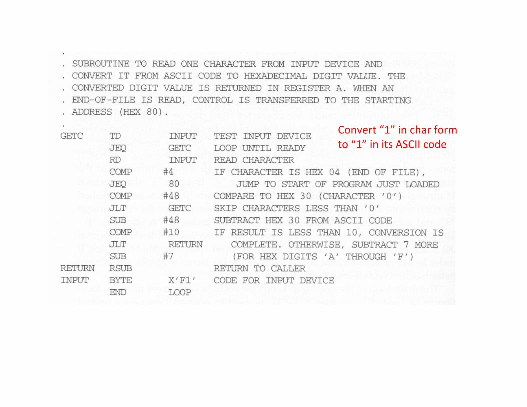
Convert “1” in char form

to “1” in its ASCII code

Relocating Loader

• Two methods to describe where in the object program to modify the address (add

the program starting address)

– Use modification records

• Suitable for a small number of changes

– Use relocation bit mask

• Suitable for a large number of changes

Program Written in SIC/XE

PC-relative

Only these three lines need

to be modified.

Base-relative

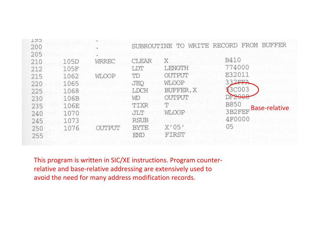
This program is written in SIC/XE instructions. Program counter-

relative and base-relative addressing are extensively used to

avoid the need for many address modification records.

Base-relative

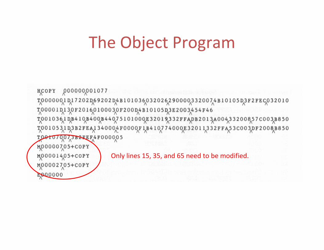
The Object Program

Only lines 15, 35, and 65 need to be modified.

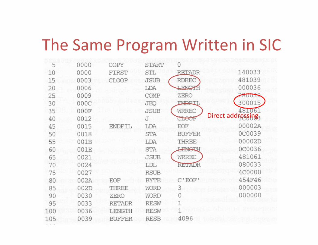
The Same Program Written in SIC

Direct addressing

Direct addressing

Direct addressing

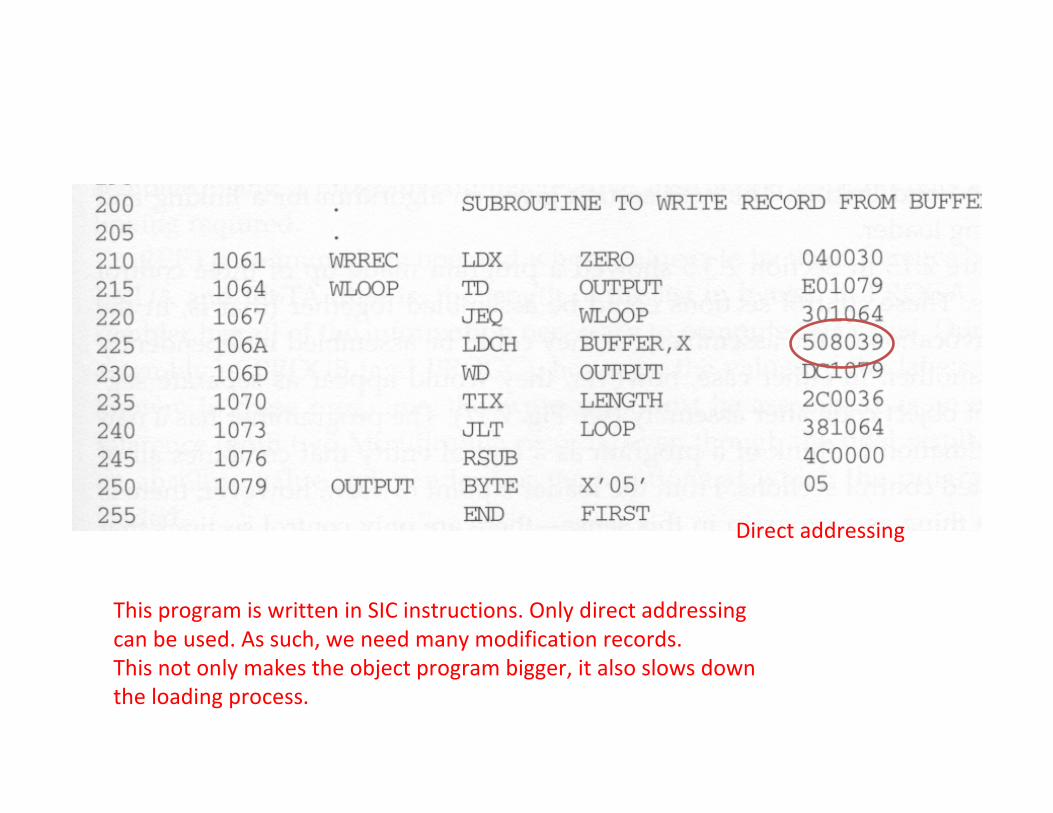
This program is written in SIC instructions. Only direct addressing

can be used. As such, we need many modification records.

This not only makes the object program bigger, it also slows down

the loading process.

Relocation Bit Mask

• If an object needs too many modification records, it would be more efficient to use a relocation bit mask to indicate where in the object program should be modified when the object program is loaded.

• A relocation bit is associated with each word of object code. Since all SIC instructions occupy one word, this means that there is one relocation bit for each possible instruction.

• If the relocation bit corresponding to a word of object code is set to 1, the program’s starting address will be added to this word when the program is relocated.

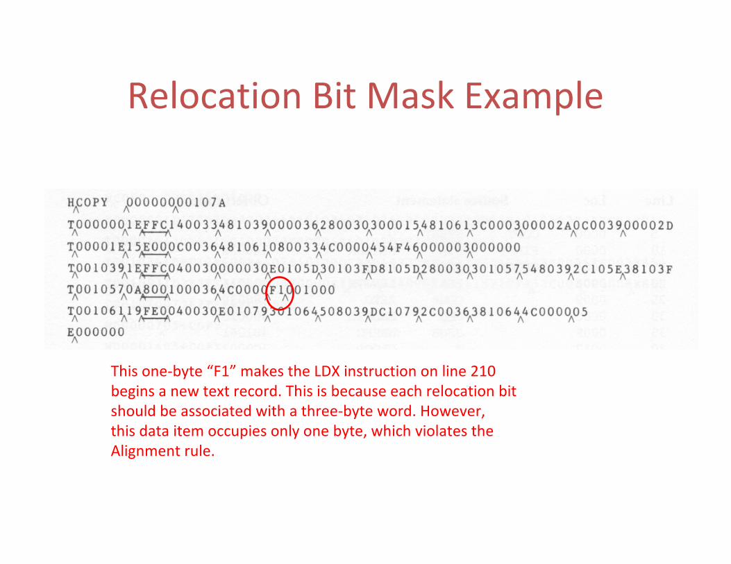
Relocation Bit Mask Example

This one-byte “F1” makes the LDX instruction on line 210

begins a new text record. This is because each relocation bit

should be associated with a three-byte word. However,

this data item occupies only one byte, which violates the

Alignment rule.

Program Linking

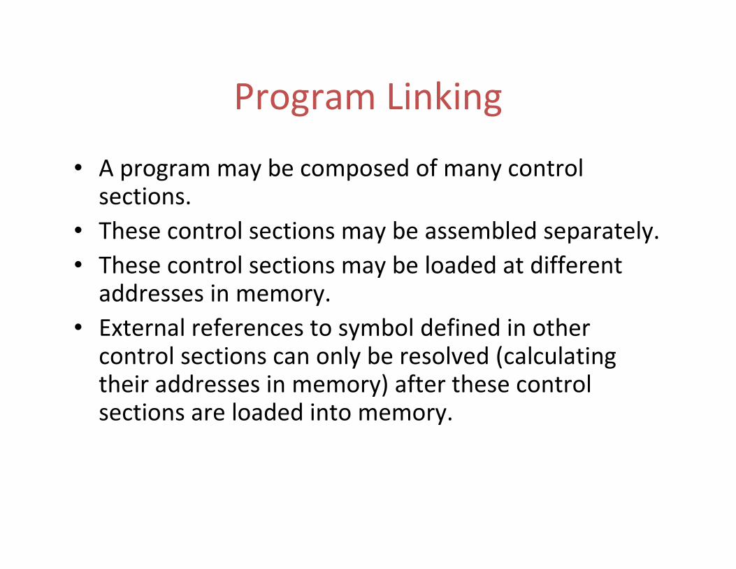
• A program may be composed of many control sections.

• These control sections may be assembled separately.

• These control sections may be loaded at different addresses in memory.

• External references to symbol defined in other control sections can only be resolved (calculating their addresses in memory) after these control sections are loaded into memory.

Program Linking Example

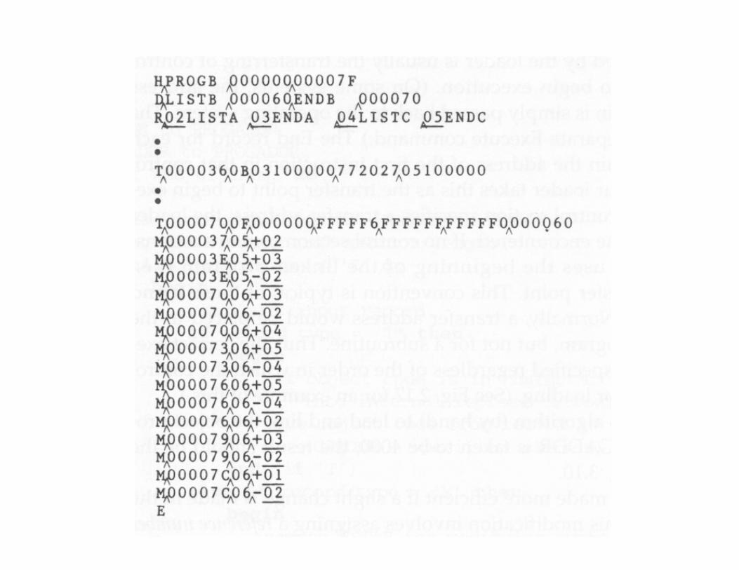
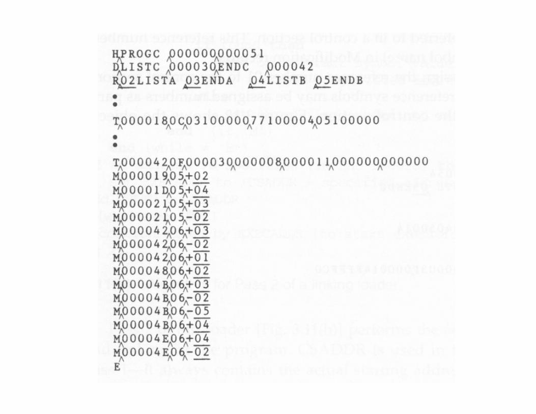
Object Program Example

Program Linking Example

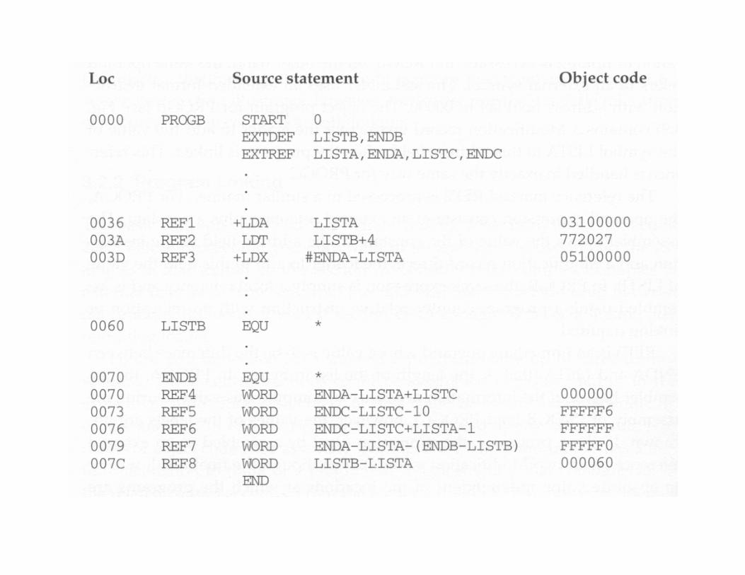
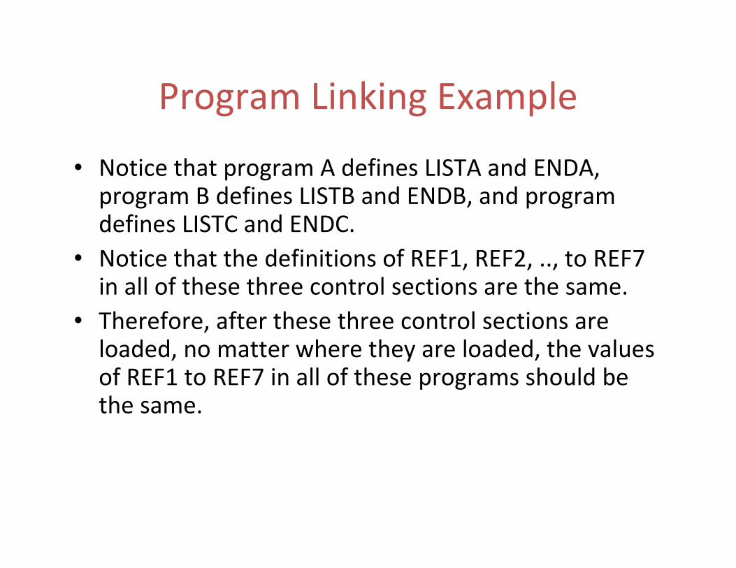
• Notice that program A defines LISTA and ENDA, program B defines LISTB and ENDB, and program defines LISTC and ENDC.

• Notice that the definitions of REF1, REF2, .., to REF7 in all of these three control sections are the same.

• Therefore, after these three control sections are loaded, no matter where they are loaded, the values of REF1 to REF7 in all of these programs should be the same.

REF1

• Program A– LISTA is defined in its own program and its address is

immediately available. Therefore, we can simply use program counter-relative addressing

• Program B– Because LISTA is an external reference, its address is not

available now. Therefore an extended-format instruction with address field set to 00000 is used. A modification record in inserted into the object code so that once LISTA’s address is known, it can be added to this field.

• Program C– The same as that processed in Program B.

REF2

• Program A– Because LISTB is an external reference, its address is not

available now. Therefore an extended-format instruction with address field set to 00004 is used. A modification record is inserted into the object code so that once LISTB’s address is available, it can be added to this field.

• Program B– LISTB is defined in its own program and its address is

immediately available. Therefore, we can simply use program counter-relative addressing

• Program C– The same as that processed in Program A.

REF3

• Program A– The difference between ENDA and LISTA (14) is

immediately available during assembly.

• Program B– Because the values of ENDA and LISTA are unknown

during assembly, we need to use an extended-format instruction with its address field set to 0.

– Two modification records are inserted to the object program – one for +ENDA and the other for –LISTA.

• Program C– The same as that processed in Program B.

REF4• Program A

– The difference between ENDA and LISTA can be known now. Only the value of LISTC is unknown. Therefore, an initial value of 000014 is stored with one modification record for LISTC.

• Program B– Because none of ENDA, LISTA, and LISTC’s values can be known

now, an initial value of 000000 is stored with three modification records for all of them.

• Program C– The value of LISTC is known now. However, the values for

ENDA and LISTA are unknown. An initial value of 000030 is stored with two modification records for ENDA and LISTA.

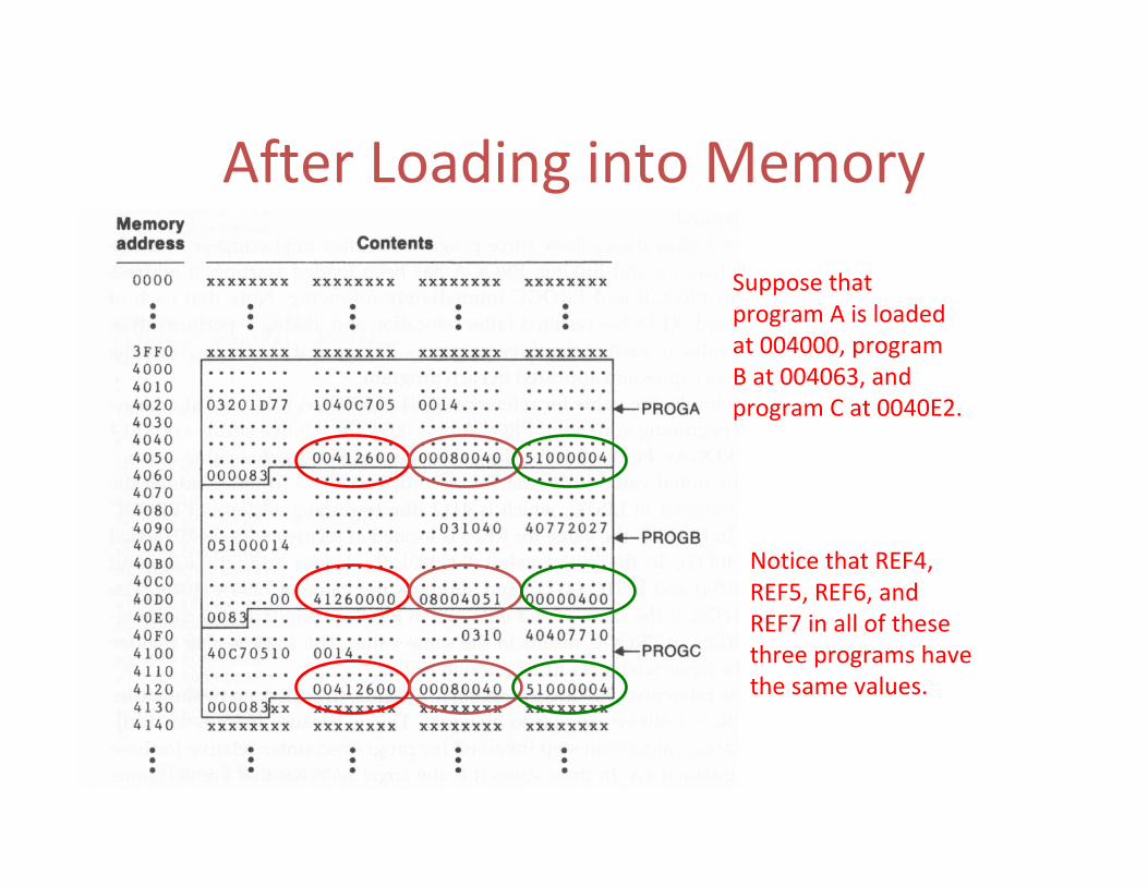
After Loading into Memory

Suppose that

program A is loaded

at 004000, program

B at 004063, and

program C at 0040E2.

Notice that REF4,

REF5, REF6, and

REF7 in all of these

three programs have

the same values.

REF4 after Linking

• Program A

– The address of REF4 is 4054 (4000 + 54) because program A is loaded at 4000 and the relative address of REF4 within program A is 54.

– The value of REF4 is 004126 because

• The address of LISTC is 0040E2 (the loaded address of program C) + 000030 (the relative address of LISTC in program C)

• 0040E2 + 000014 (constant already calculated) = 004126.

REF4 after Linking

• Program B

– The address of REF4 is 40D3 (4063 + 70) because program B is loaded at 4063 and the relative address of REF4 within program A is 70.

– The value of REF4 is 004126 because

• The address of LISTC is 004112

• The address of ENDA is 004054

• The address of LISTA is 004040

• 004054 + 004112 – 004040 = 004126

Instruction Operands

• For references that are instruction operands, the calculated values after loading do no always appear to be equal.

• This is because there is an additional address calculation step involved for program-counter (base) relative instructions.

• In such cases, it is the target addresses that are the same.

• For example, in program A, the reference REF1 is a program-counter relative instruction with displacement 1D. When this instruction is executed, the PC contains the value 4023. Therefore the resulting address is 4040. In program B, because direct addressing is used, 4040 (4000 + 40) is stored in the loaded program for REF1.

The Implementation of a Linking

Loader

• A linking loader makes two passes over its

input

– In pass 1: assign addresses to external references

– In pass 2: perform the actually loading, relocation,

and linking

• Very similar to what a two-pass assembler

does.

Data Structures

• External symbol tables (ESTAB)– Like SYMTAB, store the name and address of each external

symbol in the set of control sections being loaded.

– It needs to indicate in which control section the symbol is defined.

• PROGADDR– The beginning address in memory where the linked program is to

be loaded. (given by the OS)

• CSADDR– It contains the starting address assigned to the control section

currently being scanned by the loader.

– This value is added to all relative addresses within the controlsections.

Algorithm

• During pass 1, the loader is concerned only with HEADER and DEFINE record types in the control sections to build ESTAB.

• PROGADDR is obtained from OS.• This becomes the starting address (CSADDR) for the first control

section.• The control section name from the header record is entered into

ESTAB, with value given by CSADDR.• All external symbols appearing in the DEFINE records for the

current control section are also entered into ESTAB.• Their addresses are obtained by adding the value (offset) specified

in the DEFINE to CSADDR.• At the end, ESTAB contains all external symbols defined in the set

of control sections together with the addresses assigned to each.• A Load Map can be generated to show these symbols and their

addresses.

A Load Map

Algorithm (Cont’d)• During pass 2, the loader performs the actual loading,

relocation, and linking.• CSADDR is used in the same way as it was used in pass 1

– It always contains the actual starting address of the control section being loaded.

• As each text record is read, the object code is moved to the specified address (plus CSADDR)

• When a modification record is encountered, the symbol whose value is to be used for modification is looked up in ESTAB.

• This value is then added to or subtracted from the indicated location in memory.

Reference Number

• The linking loader algorithm can be made more efficient if we assign a reference number to each external symbol referred to in a control section.

• This reference number is used (instead of the symbol name) in modification record.

• This simple technique avoid multiple searches of ESTAB for the same symbol during the loading of a control section.

– After the first search for a symbol (the REFER records), we put the found entries into an array.

– Later in the same control section, we can just use the referencenumber as an index into the array to quickly fetch a symbol’s value.

Reference Number Example

Reference number 01 is reserved

for the current control section name.

All other reference numbers start

from 02.

Automatic Library Search

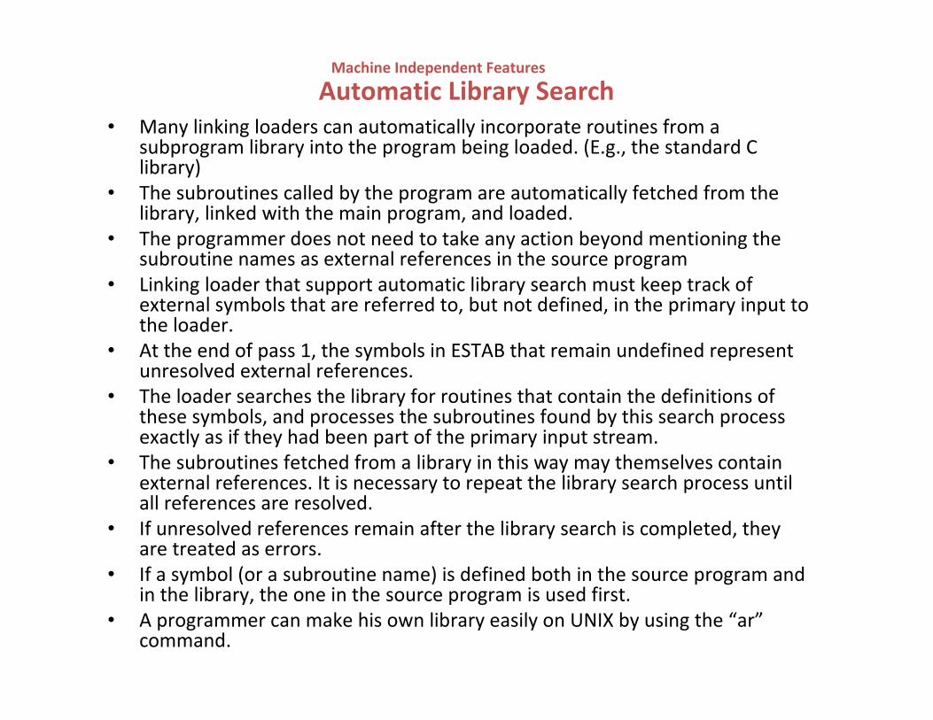
• Many linking loaders can automatically incorporate routines from a subprogram library into the program being loaded. (E.g., the standard C library)

• The subroutines called by the program are automatically fetched from the library, linked with the main program, and loaded.

• The programmer does not need to take any action beyond mentioning the subroutine names as external references in the source program

• Linking loader that support automatic library search must keep track of external symbols that are referred to, but not defined, in the primary input to the loader.

• At the end of pass 1, the symbols in ESTAB that remain undefined represent unresolved external references.

• The loader searches the library for routines that contain the definitions of these symbols, and processes the subroutines found by this search process exactly as if they had been part of the primary input stream.

• The subroutines fetched from a library in this way may themselves contain external references. It is necessary to repeat the library search process until all references are resolved.

• If unresolved references remain after the library search is completed, they are treated as errors.

• If a symbol (or a subroutine name) is defined both in the source program and in the library, the one in the source program is used first.

• A programmer can make his own library easily on UNIX by using the “ar”command.

Machine Independent Features

Loader Options

• Many loaders allow the user to specify options that modify the standard processing.

• For example:– Include program-name (library name)

• Direct the loader to read the designated object program from a library

– Delete csect-name• Instruct the loader to delete the named control sections from

the set of programs being loaded

– Change name1, name2• Cause the external symbol name1 to be changed to name2

wherever it appears in the program

Loader Options Application– In the COPY program, we write two subroutines RDREC and

WRREC to perform read records and write records.

– Suppose that the computer system provides READ and WRITE subroutines which has similar but advanced functions.

– Without modifying the source program and reassembling it, we can use the following loader options to make the COPY object program use READ rather than RDREC and WRITE rather than WRREC.

Include READ (Util)

Include WRITE (Util)

Delete RDREC, WRREC

Change RDREC, READ

Change WRREC, WRITE

Linkage Editor

• The difference between a linkage editor and a linking loader:

– A linking loader performs all linking and relocation operations, including automatic library search, and loads the linked program into memory for execution.

– A linkage editor produces a linked version of the program, which is normally written to a file for later execution.

Loader Design Options

Linkage Editor

• When the user is ready to run the linked program, a simple relocating loader can be used to load the program into memory.

• The only object code modification necessary is the addition of an actual address to relative values within the program.

• The linkage editor performs relocation of all control sections relative to the start of the linked program.

• All items that need to be modified at load time have values that are relative to the start of the linked program.

• This means that the loading can be accomplished in one pass with no external symbol table required.

• Thus, if a program is to be executed many times without being reassembled, the use of a linkage editor can substantially reduces the overhead required.

– Resolution of external references and library searching are onlyperformed once.

Dynamic Linking

• Linkage editors perform linking before the program is loaded for execution.

• Linking loaders perform these same operations at load time.

• Dynamic linking postpones the linking function until execution time.

– A subroutine is loaded and linked to the test of the program when it is first called.

• Dynamic linking is often used to allow several executing programs to share one copy of a subroutine or library.

• For example, a single copy of the standard C library can be loaded into memory.

• All C programs currently in execution can be linked to this one copy, instead of linking a separate copy into each object program.

• In an object-oriented system, dynamic linking is often used for references to

software object.

• This allows the implementation of the object and its method to be determined at

the time the program is run. (e.g., C++)

• The implementation can be changed at any time, without affecting the program

that makes use of the object.

Dynamic Linking Advantage

• The subroutines that diagnose errors may never

need to be called at all.

• However, without using dynamic linking, these

subroutines must be loaded and linked every time

the program is run.

• Using dynamic linking can save both space for storing

the object program on disk and in memory, and time

for loading the bigger object program.

On PC Windows or UNIX operating

systems, normally you are using (e.g., ld)

a linkage editor to generate an

executable program.

Dynamic Linking Implementation

• A subroutine that is to be dynamically loaded must be called via an operating system service request.

– This method can also be thought of as a request to a part of the loader that is kept in memory during execution of the program

• Instead of executing a JSUB instruction to an external symbol, the program makes a load-and-call service request to the OS.

• The parameter of this request is the symbolic name of the routine to be called.

• The OS examines its internal tables to determines whether the subroutine is already loaded.

• If needed, the subroutine is loaded from the library.

• Then control is passed from the OS to the subroutine being called.

• When the called subroutine completes its processing, it returns to its caller (operating system).

• The OS then returns control to the program that issues the request.

• After the subroutine is completed, the memory that was allocated to it may be released.

• However, often this is not done immediately. If the subroutine is retained in

memory, it can be used by later calls to the same subroutine without loading the

same subroutine multiple times.

• Control can simply pass from the dynamic loader to the called routine directly.

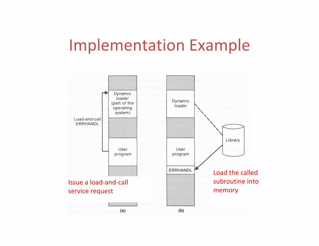
Implementation Example

Issue a load-and-call

service request

Load the called

subroutine into

memory

The called subroutine

this time is already loaded.

Control is passed

to the loaded

subroutine.

Control is returned

to the loader and

later returned to

the user program

Macro Processors

Introduction

• A macro represents a commonly used group of

statements in the source programming language

• The macro processor replaces each macro

instruction with the corresponding group of source

language statement, this is called expanding macros

• The functions of a macro processor essentially

involve the substitution of one group of characters

or lines for another

Macro Definition and Expansion

• The MACRO statement identifies the beginning of a macro definition

• The symbol in the label field is the name of the instruction

• The entries in the operand field identify the parameter of the macro instruction

• Each parameter begins with the character &

• The MEND assembler directive marks the end of the macro definition

• A macro invocation statement gives the name of the macro instruction being invoked and the arguments to be used in expanding the macro

Use of macros in a SIC/XE Program(3/1)

Use of macros in a SIC/XE Program(3/2)

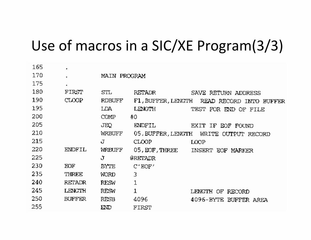
Use of macros in a SIC/XE Program(3/3)

Program with Macro Expanded(3/1)

Program with Macro Expanded(3/2)

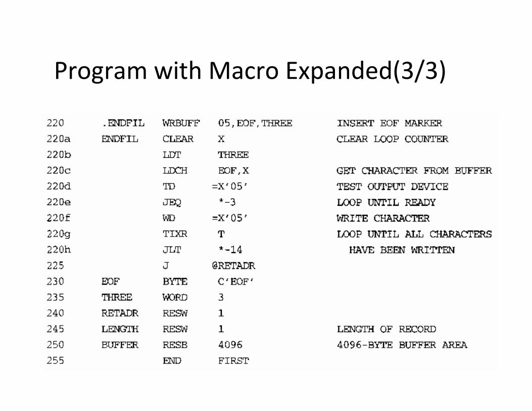
Program with Macro Expanded(3/3)

Macro Processor Data Structures

• The macro definitions themselves are stored in definition table (DEFTAB), which contains the macro prototype and the statements that make up the macro body

• The macro names are entered into NAMTAB, which serves as an index to DEFTAB

• For each macro instruction defined NAMTAB contains pointers to the beginning and end of the definition in DEFTAB

• The third data structure is an argument table (ARGTAB), which is used during the expansion of macro invocations

• When a macro invocation statement is recognized, the arguments are stored in ARGTAB according to their position in the argument list

Macro Processor Data Structures

Algorithm for a One-pass Macro

Processor(3/1)

Algorithm for a One-pass Macro

Processor(3/2)

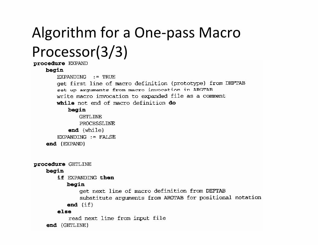
Algorithm for a One-pass Macro

Processor(3/3)

Concatenation of Macro Parameters(2/1)

• Most macro processors allow parameters to concatenated with other character strings

• If similar processing is to be performed on each series of variables, the programmer might want to incorporate this processing in to a macro instruction

• The body of the macro definition might contain a statement like “LDA X&ID1” in which the parameter &ID is concatenated after the character string X and before the character string 1

• If the macro definition contained both &ID and &ID1 as parameters, the situation would be ambiguous

• Most macro processors deal with this problem by providing a special concatenation operator (e.g. �)

• LDA X&ID�1

Concatenation of Macro

Parameters(2/2)

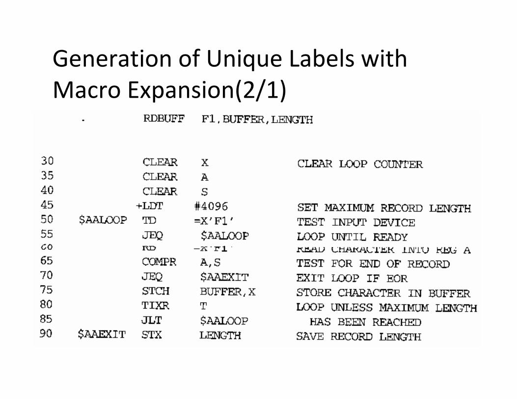
Generation of Unique Labels

• Relative addressing in a source statement may be acceptable for short jumps such as “JEQ *-3*

• For longer jumps spanning several instructions, such notation is very inconvenient, error-prone and difficult to read

• Allow the creation of special types of labels

• Each symbol beginning with $ has been modified by replacing $ with $xx, where xx is a two character alphanumeric counter of the number of macro instructions expanded

• For the first macro expansions, xx will have the value AA

• For succeeding macro expansions, xx will be set to AB, AC, etc

Generation of Unique Labels with Macro

Expansion(2/1)

Generation of Unique Labels with

Macro Expansion(2/1)

Conditional Macro Expansion(2/1)

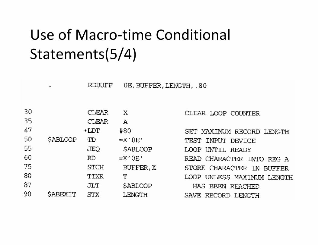
• Most macro processors can modify the sequence of statements generated for a macro expansion, depending on the arguments supplied in the macro invocation

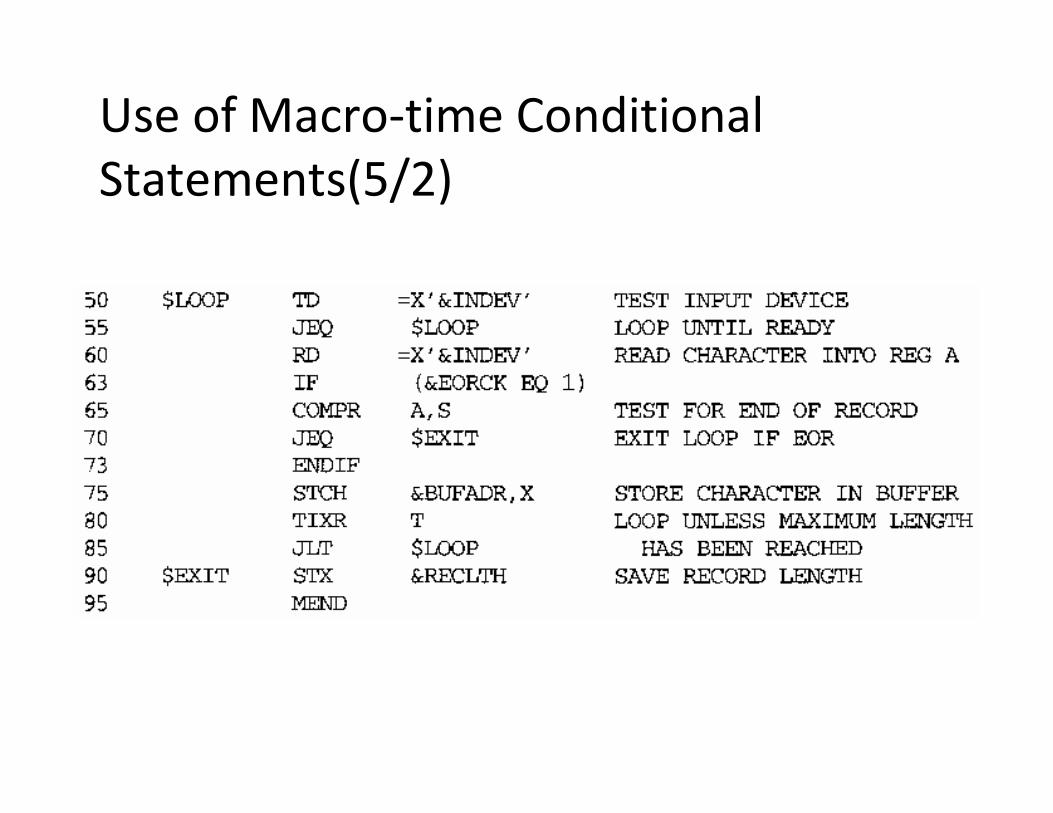
• The IF statement evaluates a Boolean expression that is its operand

• If the value of this expression is TRUE, the statements following the IF are generated until an ELSE is encountered

• Otherwise, these statements are skipped, and the statements following the ELSE are generated

• The ENDIF statement terminates the conditional expression that was begun by the IF statement

Conditional Macro Expansion(2/2)

• The macro processor must maintain a symbol table that contains the values of all macro-time variables used

• Entries in this table are made or modified when SET statements are processed

• The implementation outlined above does not allow for nested IF structures

• WHILE: a macro-time looping statement

• The WHILE statement specifies that the following lines, until the next ENDW statement, are to be generated repeatedly as long as a particular condition is true

• The macro-time variable &CTR is used to count the number of times the lines following the WHILE statement have been generated

Use of Macro-time Conditional

Statements(5/1)

Use of Macro-time Conditional

Statements(5/2)

Use of Macro-time Conditional

Statements(5/3)

RDBUFF F3, BUF, RECL, 04, 2048

Use of Macro-time Conditional

Statements(5/4)

Use of Macro-time Conditional

Statements(5/5)

Use of Macro-time looping Statements(2/1)

Use of Macro-time looping

Statements(2/2)

Keyword Macro Parameters

• Positional parameter: parameters and arguments were associated with each other according to their positions in the macro prototype and the macro invocation statement

• Keyword parameters: each argument value is written with a keyword that named the corresponding parameter

• Each parameter name is followed by an equal sign, which identifies a keyword parameter

• The parameter is assumed to have the default value if its name does not appear in the macro invocation statement

Use of Keyword Parameters in Macro

Instructions(3/1)

Use of Keyword Parameters in Macro

Instructions(3/2)

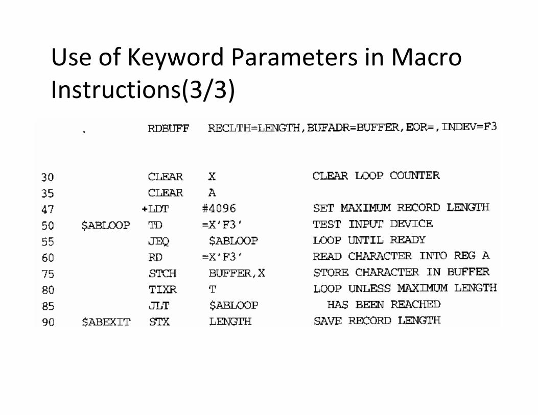
Use of Keyword Parameters in Macro

Instructions(3/3)

Macro Processor Design Options

• Recursive Macro expression

• General-Purpose Macro Processors

• Macro Processing within Language Translators

Recursive Macro Expansion

• Macro within macro can be solved if the macro processor is being written in a programming language that allows recursive calls

• The compiler would be sure that previous value of any variables declared within a procedure were saved when that procedure was called recursively

• If would take care of other details involving return from the procedure

Example of Nested Macro Invocation(2/1)

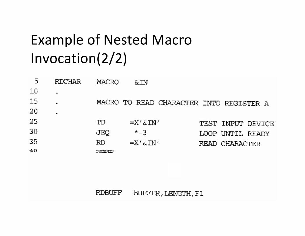
Example of Nested Macro

Invocation(2/2)

General-Purpose Macro Processors(2/1)

• Advantages of general-purpose macro processors:– The programmer does not need to learn about a different

macro facility for each compiler or assembler language—the time and expense involved in training are eliminated

– The costs involved in producing a general-purpose macro processor are somewhat greater than those for developing a language-specific processor

– However, this expense does not need to be repeated for each language; the result is substantial overall saving in software development cost

General-Purpose Macro Processors(2/2)

• A general-purpose facility must provide some way for a user to define the specific set of rules to be followed

• Comments should usually be ignored by a macro processor, however, each programming language has its own methods for identifying comments

• Each programming language has different facilities for grouping terms, expressions, or statements—a general-purpose macro processor needs to taking these grouping into account

• Languages differ substantially in their restrictions on the length of identifiers and the rules for the formation of constants

• Programming languages have different basic statement forms—syntax used for macro definitions and macro invocation statements

Macro Processing within Language

Translators(2/1)

• The macro processor reads the source statements and performs all of its functions, the output lines are passed to the language translator as they are generated

• The macro processor operates as a sort of input routine for the assembler or compiler

• The line-by-line approach avoids making an extra pass over the source program, so it can be more efficient than using a macro preprocessor

• Some of the data structures required by the macro processor and the language translator can be combined

• A line-by-line macro processor also makes it easier to give diagnostic messages that are related to the source statement containing the error

Macro Processing within Language

Translators(2/2)

• An integrated macro processor can potentially make use of any information about the source program that is extracted by the language translator

• An integrated macro processor can support macro instructions that depend upon the context in which they occur

• Line-by-line macro processors must be specially designed and written to work with a particular implementation of an assembler or compiler, which results in a more expensive piece of software

• The assembler or compiler will be considerably larger and more complex than it would be

• The additional complexity will add to the overhead of language translation

Introduction to Compilers

Compilers and Interpreters

• “Compilation”

– Translation of a program written in a source

language into a semantically equivalent program

written in a target language

– Oversimplified view:

156

Compiler

Error messages

Source

ProgramTarget

Program

Input

Output

Compilers and Interpreters

(cont’d)

• “Interpretation”

– Performing the operations implied by the source

program

– Oversimplified view:

157

Interpreter

Source

Program

Input

Output

Error messages

Compilers and Interpreters

(cont’d)

• Compiler: a program that translates an

executable program in one language into an

executable program in another language

• Interpreter: a program that reads an

executable program and produces the results

of running that program

158

The Analysis-Synthesis Model of

Compilation

• There are two parts to compilation:

– Analysis

• Breaks up source program into pieces and imposes a

grammatical structure

• Creates intermediate representation of source

program

• Determines the operations and records them in a tree

structure, syntax tree

• Known as front end of compiler

159

The Analysis-Synthesis Model of

Compilation (cont’d)– Synthesis

• Constructs target program from intermediate

representation

• Takes the tree structure and translates the

operations into the target program

• Known as back end of compiler

160

Other Tools that Use the Analysis-

Synthesis Model

• Editors (syntax highlighting)

• Pretty printers (e.g. Doxygen)

• Static checkers (e.g. Lint and Splint)

• Interpreters

• Text formatters (e.g. TeX and LaTeX)

• Silicon compilers (e.g. VHDL)

• Query interpreters/compilers (Databases)

161

A language-processing system

162

Preprocessor

Compiler

Assembler

Linker

Skeletal Source Program

Source Program

Target Assembly Program

Relocatable Object Code

Absolute Machine Code

Libraries and

Relocatable Object Files

Try for example:

gcc -v myprog.c

Analysis

• In compiling, analysis has three phases:

– Linear analysis: stream of characters read from

left-to-right and grouped into tokens; known as

lexical analysis or scanning

– Hierarchical analysis: tokens grouped

hierarchically with collective meaning; known as

parsing or syntax analysis

– Semantic analysis: check if the program

components fit together meaningfully

163

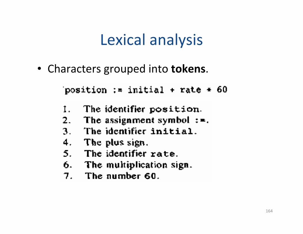
Lexical analysis

• Characters grouped into tokens.

164

Syntax analysis (Parsing)

• Grouping tokens into grammatical phrases

• Character groups recorded in symbol table

• Represented by a parse tree

165

Syntax analysis (cont’d)

• Hierarchical structure usually expressed by

recursive rules

• Rules for definition of expression:

166

Semantic analysis

• Checks source program for semantic errors

• Gathers type information for subsequent code

generation (type checking)

• Identifies operator and operands of

expressions and statements

167

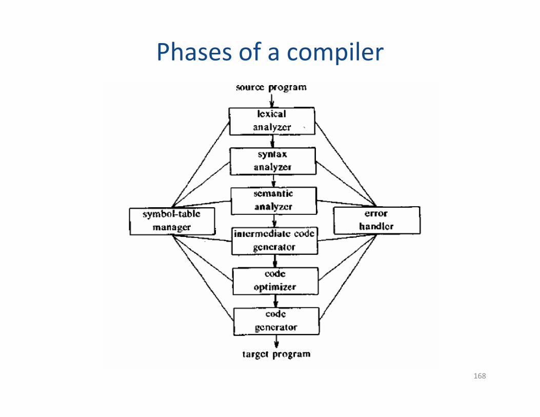
Phases of a compiler

168

Symbol-Table Management

• Symbol table – data structure with a record

for each identifier and its attributes

• Attributes include storage allocation, type,

scope, etc

• All the compiler phases insert and modify the

symbol table

169

Intermediate code generation

• Program representation for an abstract

machine

• Should have two properties

– Easy to produce

– Easy to translate into target program

• Three-address code is a commonly used form

– similar to assembly language

170

Code optimization and generation

• Code Optimization

– Improve intermediate code by producing code

that runs faster

• Code Generation

– Generate target code, which is machine code or

assembly code

171

The Phases of a Compiler

172

Phase Output Sample

Programmer (source code producer) Source string A=B+C;

Scanner (performs lexical analysis) Token string ‘A’, ‘=’, ‘B’, ‘+’, ‘C’, ‘;’

And symbol table with names

Parser (performs syntax analysis

based on the grammar of the

programming language)

Parse tree or abstract syntax tree ;

|

=

/ \

A +

/ \

B C

Semantic analyzer (type checking,

etc)

Annotated parse tree or abstract

syntax tree

Intermediate code generator Three-address code, quads, or

RTL

int2fp B t1

+ t1 C t2

:= t2 A

Optimizer Three-address code, quads, or

RTL

int2fp B t1

+ t1 #2.3 A

Code generator Assembly code MOVF #2.3,r1

ADDF2 r1,r2

MOVF r2,A

The Grouping of Phases

• Compiler front and back ends:

– Front end:

• Analysis steps + Intermediate code generation

• Depends primarily on the source language

• Machine independent

– Back end:

• Code optimization and generation

• Independent of source language

• Machine dependent

173

The Grouping of Phases (cont’d)

• Compiler passes:

– A collection of phases is done only once (single pass) or

multiple times (multi pass)

• Single pass: reading input, processing, and producing output by

one large compiler program; usually runs faster

• Multi pass: compiler split into smaller programs, each making a

pass over the source; performs better code optimization

174