system simulation modeling mca and be notes
TRANSCRIPT

System Simulation & Modeling Sushil Gupta
CHAPTER - 1
INTRODUCTION TO SIMULATION
1 th th
Sushil Gupta
Simulation
A Simulation is the imitation of the operation of a real-world process or system over
time.
Brief Explanation
• The behavior of a system as it evolves over time is studied by developing a simulation
model.
• This model takes the form of a set of assumptions concerning the operation of the system.
The assumptions are expressed in
° Mathematical relationships
° Logical relationships
° Symbolic relationships
Between the entities of the system.
Measures of performance
The model solved by mathematical methods such as differ ential calculus, probability
theory, algebraic methods has the solution usually consists of one or more numerical parameters
which are called measures of performance.
1.1 When Simulation is the Appropriate Tool
• Simulation enables the study of and experimentation with the internal interactions of a
complex system, or of a subsystem within a complex system.
• Informational, organizational and environmental changes can be simulated and the effect
of those alternations on the model‘s behavior can be observer.
• The knowledge gained in designing a simulation model can be of great value toward
suggesting improvement in the system under investigation.
• By changing simulation inputs and observing the resulting outputs, valuable insight may
be obtained into which variables are most important and how variables interact.
• Simulation can be used as a pedagogical device to reinforce analytic solution
methodologies.
2 th th
Sushil Gupta
• Simulation can be used to experiment with new designs or policies prior to
implementation, so as to prepare for what may happen.
• Simulation can be used to verify analytic solutions.
• By simulating different capabilities for a machine, requirements can be determined.
• Simulation models designed for training, allow learning without the cost and disruption
of on-the-job learning.
• Animation shows a system in simulated operation so that the plan can be visualized.
• The modern system(factory, water fabrication plant, service organization, etc) is so
complex that the interactions can be treated only through simulation.
1.2 When Simulation is Not Appropriate
• Simulation should be used when the problem cannot be solved using common sense.
• Simulation should not be used if the problem can be solved analytically.
• Simulation should not be used, if it is easier to perform direct experiments.
• Simulation should not be used, if the costs exceeds savings.
• Simulation should not be performed, if the resources or time are not available.
• If no data is available, not even estimate simulation is not advised.
• If there is not enough time or the person are not available, simulation is not appropriate.
• If managers have unreasonable expectation say, too much soon – or the power of
simulation is over estimated, simulation may not be appropriate.
• If system behavior is too complex or cannot be defined, simulation is not appropriate.
1.3 Advantages o f Simulation
• Simulation can also be used to study systems in the design stage.
• Simulation models are run rather than solver.
• New policies, operating procedures, decision rules, information flow, etc can be explored
without disrupting the ongoing operations of the real system.
3 th th
Sushil Gupta
• New hardware designs, physical layouts, transportation systems can be tested without
committing resources for their acquisition.
• Hypotheses about how or why certain phenomena occur can be tested for feasibility.
• Time can be compressed or expanded allowing for a speedup or slowdown of the
phenomena under investigation.
• Insight can be obtained about the interaction of variables.
• Insight can be obtained about the importance of variables to the performance of the
system.
• Bottleneck analysis can be performed indication where work- inprocess, information
materials and so on are being excessively delayed.\
• A simulation study can help in understanding how the system operates rather than how
individuals think the system operates.
• ―what-if‖ questions can be answered. Useful in the design of new systems.
1.4 Disadvantages of simulation
• Model building requires special training.
• Simulation results may be difficult to interpret.
• Simulation modeling and analysis can be time consuming and expensive.
• Simulation is used in some cases when an analytical solution is possible or even
preferable.
1.5 Applications of Simulation
Manufa cturing Applications
1. Analysis of electronics assembly operations
2. Design and evaluation of a selective assembly station for highprecision scroll
compressor shells.
3. Comparison of dispatching rules for semiconductor manufacturing using large facility
models.
4. Evaluation of cluster tool throughput for thin-film head production.
4 th th

Sushil Gupta
5. Determining optimal lot size for a semiconductor backend factory.
6. Optimization of cycle time and utilization in semiconductor test manufacturing.
7. Analysis of storage and retrieval strategies in a warehouse.
8. Investigation of dynamics in a service oriented supply chain.
9. Model for an Army chemical munitions disposal facility.
Semiconductor Manufacturing
1. Comparison of dispatching rules using large-facility models.
2. The corrupting influence of variability.
3. A new lot-release rule for wafer fabs.
4. Assessment of potential gains in productivity due to proactive retied management.
5. Comparison of a 200 mm and 300 mm X-ray lithography cell.
6. Capacity planning with time constraints between operations.
7. 300 mm logistic system risk reduction.
Construction Engineering
1. Construction of a dam embankment.
2. Trench less renewal of underground urban infrastructures.
3. Activity scheduling in a dynamic, multiproject setting.
4. Investigation of the structural steel erection process.
5. Special purpose template for utility tunnel construction.
Military Applicatio ns
1. Modeling leadership effects and recruit type in a Army recruiting station.
2. Design and test of an intelligent controller for autonomous underwater vehicles.
3. Modeling military requirements for nonwarfighting operations.
5 th th

Sushil Gupta
4. Multitrajectory performance for varying scenario sizes.
5. Using adaptive agents in U.S. Air Force retention.
Logistics, Transportation and Distribution Applica tions
1. Evaluating the potential benefits of a rail-traffic planning algorithm.
2. Evaluating strategies to improve railroad performance.
3. Parametric Modeling in rail-capacity planning.
4. Analysis of passenger flows in an airport terminal.
5. Proactive flight-schedule evaluation.
6. Logistic issues in autonomous food production systems for extended duration space
exploration.
7. Sizing industrial rail-car fleets.
8. Production distribution in newspaper industry.
9. Design of a toll plaza
10. Choosing between rental-car locations.
11. Quick response replenishment.
Business Process Simulation
1. Impact of connection bank redesign on airport gate assignment.
2. Product development program planning.
3. Reconciliation of business and system modeling.
4. Personal forecasting and strategic workforce planning.
Human Systems
1. Modeling human performance in complex systems.
2. Studying the human element in out traffic control.
6 th th
Sushil Gupta
1.6 Systems
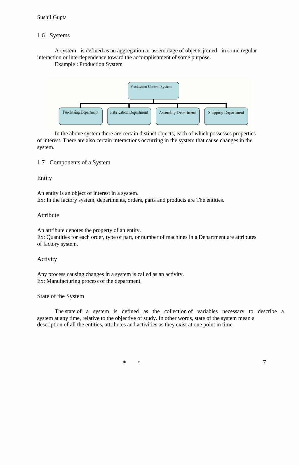
A system is defined as an aggregation or assemblage of objects joined in some regular
interaction or interdependence toward the accomplishment of some purpose.
Example : Production System
In the above system there are certain distinct objects, each of which possesses properties
of interest. There are also certain interactions occurring in the system that cause changes in the
system.
1.7 Components of a System
Entity
An entity is an object of interest in a system.
Ex: In the factory system, departments, orders, parts and products are The entities.
Attribute
An attribute denotes the property of an entity.
Ex: Quantities for each order, type of part, or number of machines in a Department are attributes
of factory system.
Activity
Any process causing changes in a system is called as an activity.
Ex: Manufacturing process of the department.
State of the System
The state of a system is defined as the collection of variables necessary to describe a
system at any time, relative to the objective of study. In other words, state of the system mean a
description of all the entities, attributes and activities as they exist at one point in time.
7 th th
Sushil Gupta
Event
An event is define as an instaneous occurrence that may change the
state of the system.
1.8 System Environment
The external components which interact with the system and produce necessary changes
are said to constitute the system environment. In modeling systems, it is necessary to decide on
the boundary between the system and its environment. This decision may depend on the purpose
of the study.
Ex: In a factory system, the factors controlling arrival of orders may be considered to be outside
the factory but yet a part of the system environment. When, we consider the demand and supply
of goods, there is certainly a relationship between the factory output and arrival of orders. This
relationship is considered as an activity of the system.
Endogenous System
The term endogenous is used to describe activities and events occurring within a system. Ex: Drawing cash in a bank.
Exogenous System
The term exogenous is used to descr ibe activities and events in the environment that
affect the system. Ex: Arrival of customers.
Closed System
A system for which there is no exogenous activity and event is said to be a closed. Ex:
Water in an insulated flask.
Open system
A system for which there is exogenous activity and event is said to be a open. Ex: Bank
system.
Discrete and Continuous Systems
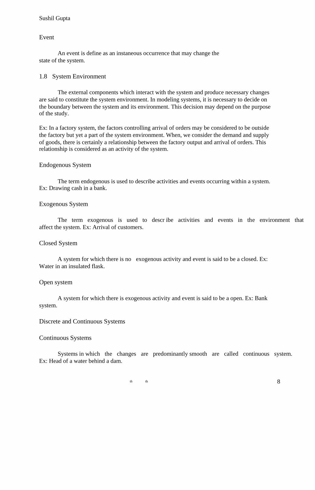
Continuous Systems
Systems in which the changes are predominantly smooth are called continuous system.
Ex: Head of a water behind a dam.
8 th th
Sushil Gupta
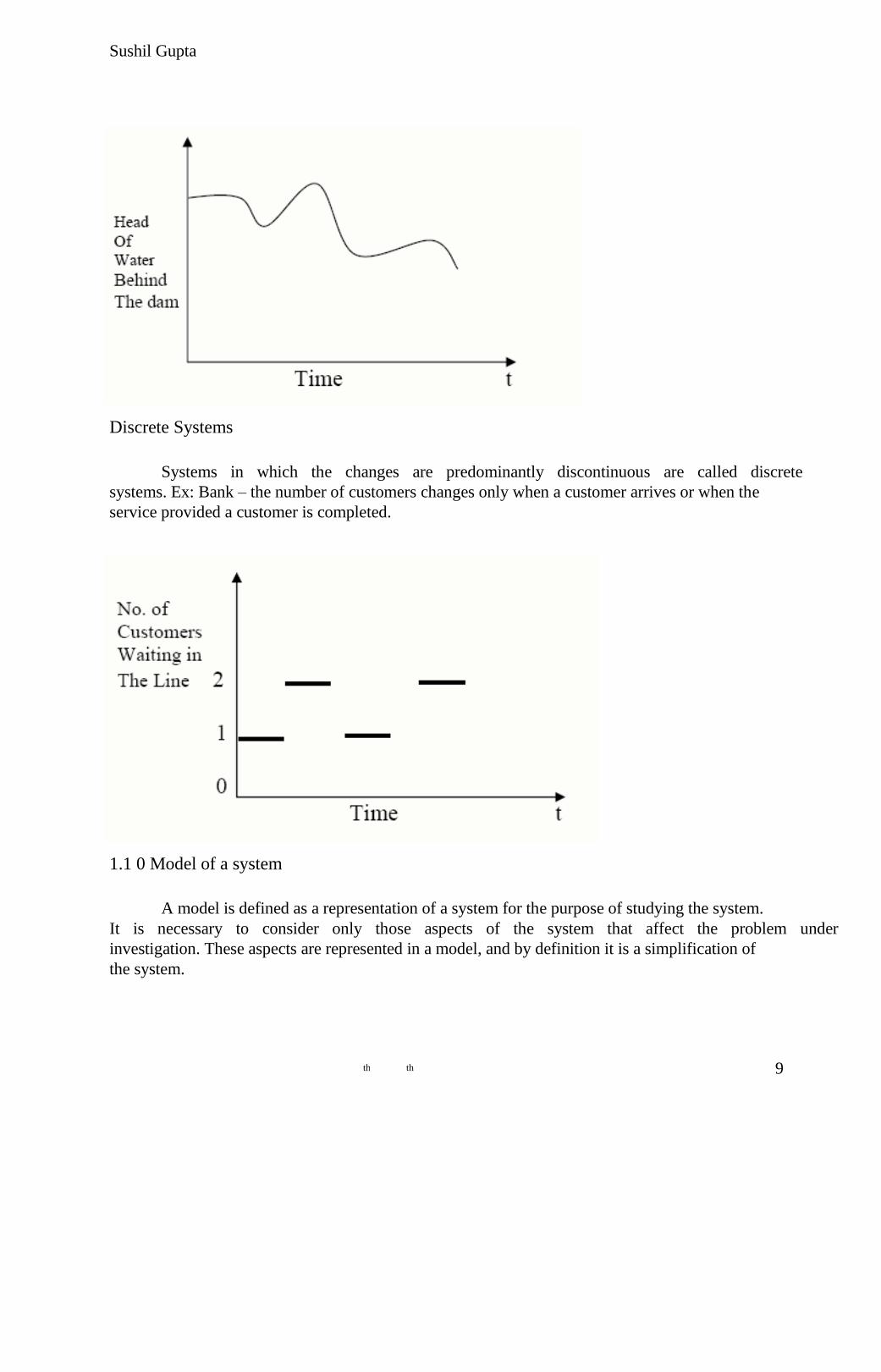
Discrete Systems
Systems in which the changes are predominantly discontinuous are called discrete
systems. Ex: Bank – the number of customers changes only when a customer arrives or when the
service provided a customer is completed.
1.1 0 Model of a system
A model is defined as a representation of a system for the purpose of studying the system.
It is necessary to consider only those aspects of the system that affect the problem under
investigation. These aspects are represented in a model, and by definition it is a simplification of
the system.
9 th th
Sushil Gupta
1.1 1 Types of Models
The various types models are
• Mathematical or Physical Model
• Static Model
• Dynamic Model
• Deterministic Model
• Stochastic Model
• Discrete Model
• Continuous Mod el
Mathematical Model
Uses symbolic notation and the mathematical equations to represent a
system.
Static Model
Rep resents a system at a particular p oint of time and also known as Monte-
Carlo simulation.
Dynamic Model
Rep resents systems as they change over time. Ex: Simulation of a bank
Deterministic Model
Contains no random variables. They have a known set of inputs which will
result in a unique set of outputs. Ex: Arrival of patients to the Dentist at the
scheduled appointment time.
Stochastic Model
Has one or mo re random variable as inputs. Random inputs leads to random
outputs. Ex: Simulation of a bank involv es ran dom interarrival and service times.
10 th th
Sushil Gupta
Discrete and Continuous Model
Used in an an alogous manner. Simulation models may be mixed both with
discrete and continuous. The choice is based on the characteristics of the system
and the objective of the study.
1.1 2 Discrete-Event System Simulation
Modeling of systems in which the state variable changes only at a discrete
set of points in time. The simulation models are analyzed by numerical rather than
by analytical methods. An alytical methods employ the deductive reasoning of
mathematics to solve th e model. Eg: Differential calculus can be used to determine
the minimum cost policy for some inventory models.
Numerical methods use computational procedures and are ‗runs‘, which is
generated based on th e model assumptions an d observations are collected to be
analyzed and to estimate the true system performance measures. Real-world
simulation is so vast, whose runs are conducted with the help of compu ter. Much
insight can be o btained by simulation manually which is applicable for small
systems.
1.1 3 Steps in a Simulation study
1. Problem formulation
Every study begins with a statement of the problem, provided by policy
makers. Analyst ensures its clearly understood. If it is developed by analyst policy
makers should understand and agree with it.
2. Setting of objectives and overall project plan
The objectives indicate the questions to be answered by simulation. At this
point a determination should be made concerning whether simulation is the
appropriate methodology. Assuming it is appropriate, the overall project plan
sho uld include
• A statement of the alternative systems
• A method for evaluating the effectiveness of these alternatives
11 th th
Sushil Gupta
• Plans for the study in terms of the number of people involved
• Cost of the study
• The number o f days required to accomplish each phase of the work with the
anticipated results.
3. Model conceptualization
The construction of a model of a system is p robably as much art as science.
The art of mo delin g is enhanced by an ability
• To abstract the essential features of a problem
• To select an d modify basic assumptions that characterize th e system
• To enrich and elaborate the model until a useful approximation results
Thus, it is best to start with a simple model and build toward greater
complexity. Model conceptualization enhance the quality of the resulting model
and increase the confidence of the model user in the application of the model.
4. Data collection
There is a constant interplay between the construction of model and the
collection of needed input data. Done in the early stages.
Objective kind of data are to be collected.
5. Model translation
Real-world systems result in models that require a great deal of information
storage and computation. It can be programmed by using simulation languages or
special purpose simulation software.
Simulation languages are powerful and flexible. Simulation software models
development time can be reduced.
6. Verified
12 th th
Sushil Gupta
It pertains to he computer program and checking the performan ce. If the
input parameters and logical structure and correctly represented, verification is
completed.
7. Validated
It is the determination that a model is an accurate representation of the real
system. Achieved through calibration of the model, an iterative p rocess of
comparing the model to actual system behavior and the discrepancies between the
two.
8. Experimental Design
The alternatives that are to be simulated must be determin ed. Which
alternatives to simulate may be a function of runs. For each system desig n,
decisions need to be made concerning
• Length of the initialization period
• Length of simulation runs
• Number of replication to be made of each run
9. Production runs and analysis
They are used to estimate measures of performance for the system designs
that are being simulated.
10. More runs
Based on the analysis of runs that have been completed. The analyst
determines if additional runs are needed and what d esign those additional
experiments should follow.
11. Documentation and repo rting
Two types of documentation.
• Program documentation
• Process documen tation
13 th th
Sushil Gupta
Program documentation
Can be used again by the same or different analysts to understand how the
program o perates. Further modification will be easier. Model users can change the
input parameters for better performance.
Process documentation
Gives the history of a simulation project. The result of all analysis should be
reported clearly and concisely in a final report. This enable to review the final
formulation and alternatives, results of the experiments and the recommended
solution to the problem. The final rep ort provides a vehicle of certification.
12. Implementation
Success d epends on the previous steps. If the model user has been
thoroughly involved an d u nderstands the nature of the model and its outputs,
likelihood of a vigorous implementatio n is enhanced.
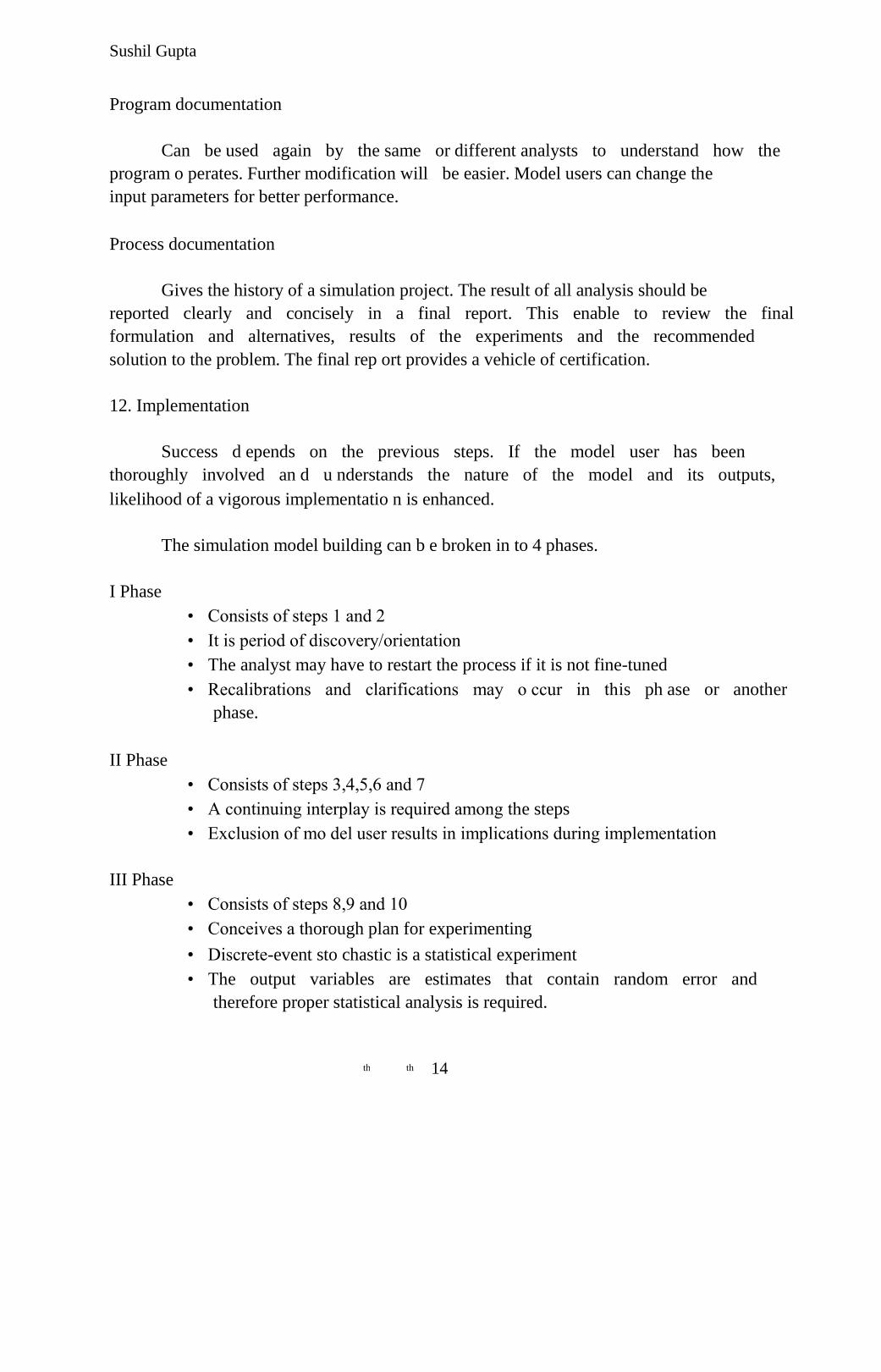
The simulation model building can b e broken in to 4 phases.
I Phase
• Consists of steps 1 and 2
• It is period of discovery/orientation
• The analyst may have to restart the process if it is not fine-tuned
• Recalibrations and clarifications may o ccur in this ph ase or another
phase.
II Phase
• Consists of steps 3,4,5,6 and 7
• A continuing interplay is required among the steps
• Exclusion of mo del user results in implications during implementation
III Phase
• Consists of steps 8,9 and 10
• Conceives a thorough plan for experimenting
• Discrete-event sto chastic is a statistical experiment
• The output variables are estimates that contain random error and
therefore proper statistical analysis is required.
14 th th
Sushil Gupta
IV Phase
• Consists of steps 11 and 12
• Successful implementatio n depends on the involvement of user and
every steps successful completion.
15 th th
Sushil Gupta
CHAPTER - 2
SIMULATION EXAMPLES
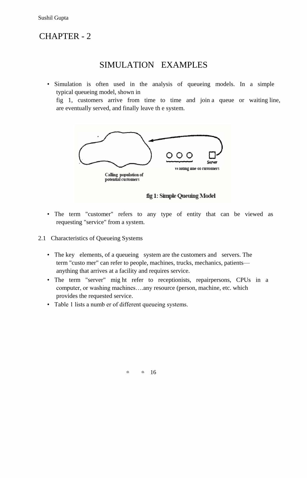
• Simulation is often used in the analysis of queueing models. In a simple
typical queueing model, shown in
fig 1, customers arrive from time to time and join a queue or waiting line,
are eventually served, and finally leave th e system.
• The term "customer" refers to any type of entity that can be viewed as
requesting "service" from a system.
2.1 Characteristics of Queueing Systems
• The key elements, of a queueing system are the customers and servers. The
term "custo mer" can refer to people, machines, trucks, mechanics, patients—
anything that arrives at a facility and requires service.
• The term "server" mig ht refer to receptionists, repairpersons, CPUs in a
computer, or washing machines….any resource (person, machine, etc. which
provides the requested service.
• Table 1 lists a numb er of different queueing systems.
16 th th

Sushil Gupta
Table 1: Examples of Queueing Systems
‹ The elements of a queuing sy stem are:-
•
•
The Calling Population:- •
•
V The population of potential customers, referred to as the calling population,
may beassumed to be finite or infinite.
V For example, consider a bank of 5 machines that are curing tires. After an
interval of time, a machine automatically opens and must b e attended by a
worker who removes the tire and puts an uncured tire into the machine. The
machines are the "customers", who "arrive" at the instant they automatically
open. The worker is the "server", who "serves" an open machine as soon as
possible. The calling population is finite, and consists of the five machines.
V In systems with a large population of potential customers, the calling
population is usually assu med to be finite or infinite. Examples of infinite
populations include the potential customers of a restaurant, bank, etc.
V The main difference between finite and infinite population models is how
the arrival rate is defined. In an infinite-population model, the arrival rate is
not affected by th e number o f customers who have left the calling population
17 th th
Sushil Gupta
and joined the queueing system. On the other hand, for finite calling
population models, the arrival rate to the queueing sy stem does depend on
the number of customers being served and waiting.
• System Capacity:-
V In many queueing systems there is a limit to the number of cu stomers that
may be in the waiting line or system. For example, an automatic car wash
may have room for only 10 cars to wait in line to enter the mechanism.
V An arriving customer who finds the system full does n ot enter but returns
immediately to the calling population.
V Some systems, such as concert ticket sales for students, may be con sidered
as having unlimited capacity. There are no limits o n the number of students
allowed to wait to purchase tickets.
V When a system has limited capacity, a distinction is made between the
arrival rate (i.e., the number of arrivals per time unit) and the effective
arrival rate (i.e., the number who arrive and enter the system per time unit).
• The Arrival Process:-
V Arrival process for infinite-population models is usually characterized in
terms of interarrival times of successive customers. Arrivals may occur at
scheduled times or at random times. When at random times, the interarrival
times are usually characterized by a probability distribu tion
V The most important model for random arrivals is the Poisson arrival process.
If An represents the interarrival time between customer n-1 and customer n
(A1 is the actual arrival time of the first customer), then for a Poisson arrival
process. An is exponentially distributed with mean I/ time Units. The
arrival rate is customers per time unit. The number of arrivals in a time
interval of length t, say N( t ) , has the Po isson distribution with mean t
customers.
V The Poisson arrival process has been successfu lly employed as a model of
the arrival of people to restaurants, drive-in banks, and other service
facilities.
V A second important class of arrivals is the scheduled arrivals, such as
patients to a physician's office or scheduled airline flight arrivals to an
18 th th
Sushil Gupta
airport. In this case, the interarrival times [An , n = 1,2,. . . } may be
constant, or constant plus or minus a small random amount to represent early
or late arrivals.
V A third situation occurs when at least one customer is assumed to always be
present in the queue, so that the server is never idle because of a lack of
customers. For example, the "custo mers" may represent raw material for a
product, and sufficient raw material is assumed to be always available.
V For finite-population models, the arrival process is characterized in a
completely different fashion. Define a customer as pending when that
customer is outside the queueing system and a member of the potential
calling population.
V Runtime of a given customer is defined as the len gth of time from departure
from the queueing system until that customer‘s next arrival to the queue.
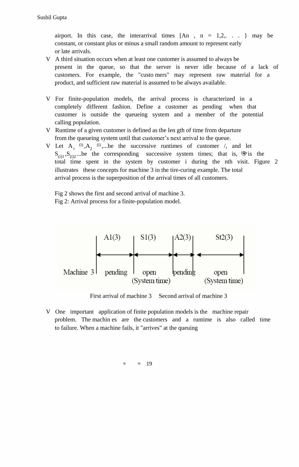
V Let A (i) ,A (i) ,...be the successive runtimes of customer /, and let i 2
S ,S ...be the corresponding successive system times; that is, S (i)n is the (i)1 (i)2
total time spent in the system by customer i during the nth visit. Figure 2
illustrates these concepts for machine 3 in the tire-curing example. The total
arrival process is the superposition of the arrival times of all customers.
Fig 2 shows the first and second arrival of machine 3.
Fig 2: Arrival process for a finite-population model.
First arrival of machine 3 Second arrival of machine 3
V One important application of finite population models is the machine repair
problem. The machin es are the customers and a runtime is also called time
to failure. When a machine fails, it "arrives" at the queuing
19 th th
Sushil Gupta
g system (the repair facility) and remains there until it is "served" (repaired).
Times to failure for a given class of machine have been ch aracterized by the
exponential, the Weibull, and the gamma distributions. Models with an
exponential runtime are sometimes analytically tractable.
• Queue Behavior and Queue Discipline:-
V Queue behavior refers to customer actions while in a queue waiting for
service to begin. In some situations, there is a possibility that incoming
customers may balk (leave when they see that the line is too long), renege
(leave after being in the line when they see that the line is moving too
slowly), or jockey (move from one line to another if they think they have
chosen a slow line).
V Queue disciplin e refers to the logical ordering of customers in a queue and
determineswhich customer will be chosen for service when a server beco mes
free.
• Common queue disciplines include first-in, first-out (FIFO); last-in
firstout (LIFO); service in random order (SIRO); shortest processing
time first |(SPT) and service according to priority (PR).
• In a job shop, queue disciplines are sometimes based on due dates and
on ex pected processing time for a given i type o f job. Notice that a
FIFO queue discipline implies that services begin in th e same order as
arrivals, but that customers may leave the system in a different order
because of differentlength service times.
• Service Times and the Service Mechanism:-
V The service times of successive arrivals are denoted by S1, S2, S3…They
may be constant or of random duration. The exponential,Weibull, gamma,
lognormal, and truncated normal distributions have all been used
successfully as models of service times in different situations.
V Sometimes services may be identically distributed for all customers of a
given type or class or priority, while customers of different types may have
completely different service-time distributions. In addition, in some systems,
service times depend upon the time of day or the leng th of the waiting line.
For example, servers may work faster than usual when the waiting line is
long, thus effectively reducing the service times.
20 th th
Sushil Gupta
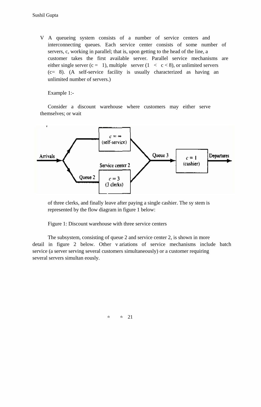
V A queueing system consists of a number of service centers and
interconnecting queues. Each service center consists of some number of
servers, c, working in parallel; that is, upon getting to the head of the line, a
customer takes the first available server. Parallel service mechanisms are
either single server (c = 1), multiple server (1 < c < 8), or unlimited servers
(c= 8). (A self-service facility is usually characterized as having an
unlimited number of servers.)
Example 1:-
Consider a discount warehouse where customers may either serve
themselves; or wait
of three clerks, and finally leave after paying a single cashier. The sy stem is
represented by the flow diagram in figure 1 below:
Figure 1: Discount warehouse with three service centers
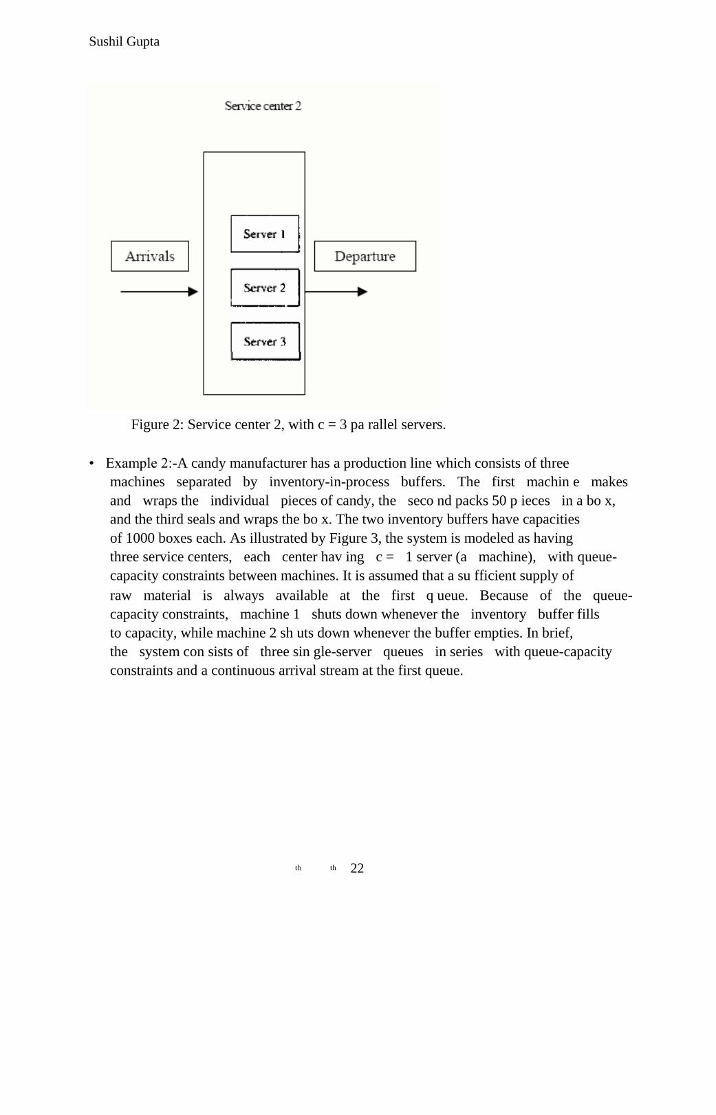
The subsystem, consisting of queue 2 and service center 2, is shown in more
detail in figure 2 below. Other v ariations of service mechanisms include batch
service (a server serving several customers simultaneously) or a customer requiring
several servers simultan eously.
21 th th
Sushil Gupta
Figure 2: Service center 2, with c = 3 pa rallel servers.
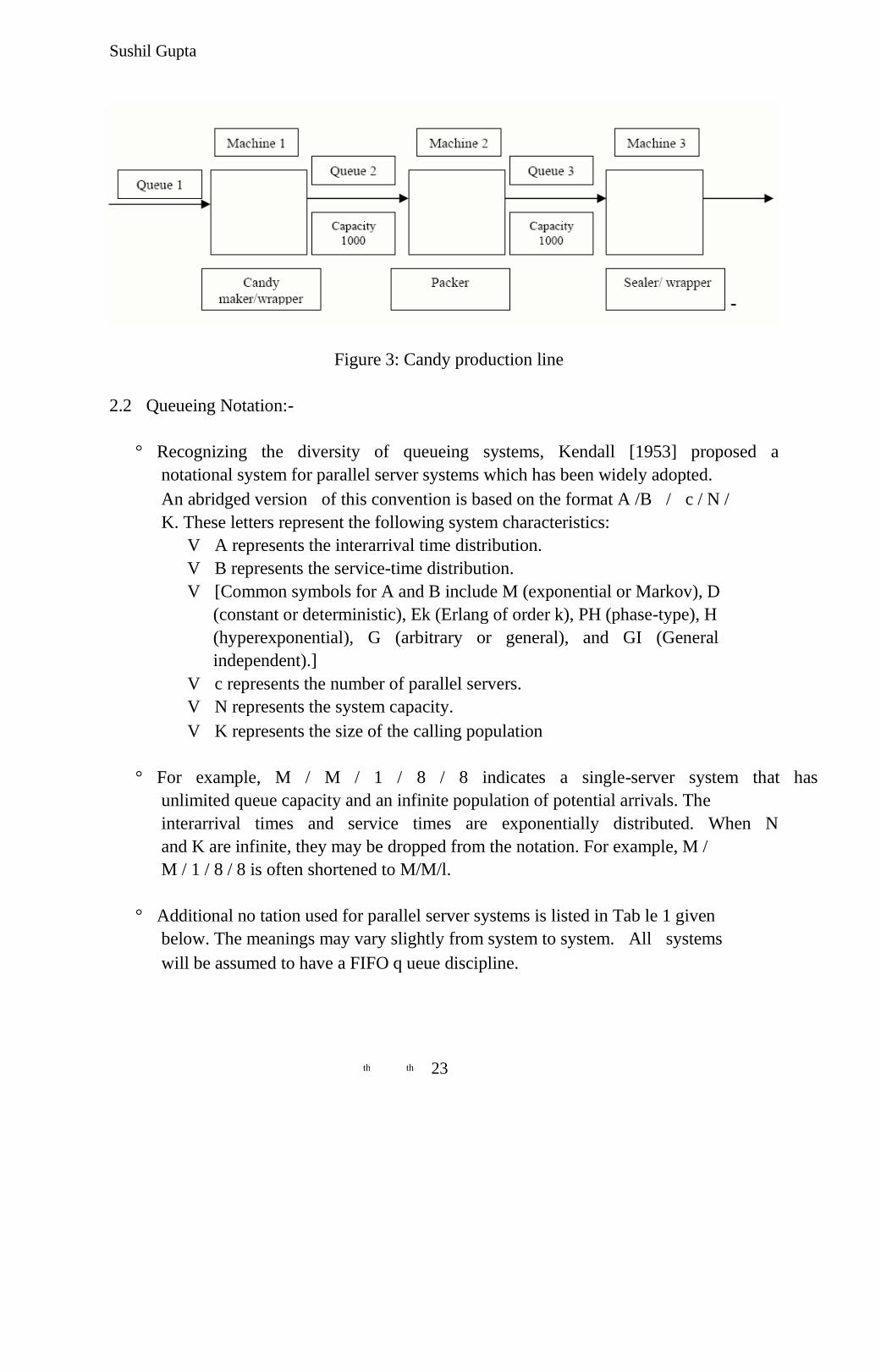
• Example 2:-A candy manufacturer has a production line which consists of three
machines separated by inventory-in-process buffers. The first machin e makes
and wraps the individual pieces of candy, the seco nd packs 50 p ieces in a bo x,
and the third seals and wraps the bo x. The two inventory buffers have capacities
of 1000 boxes each. As illustrated by Figure 3, the system is modeled as having
three service centers, each center hav ing c = 1 server (a machine), with queue-
capacity constraints between machines. It is assumed that a su fficient supply of
raw material is always available at the first q ueue. Because of the queue-
capacity constraints, machine 1 shuts down whenever the inventory buffer fills
to capacity, while machine 2 sh uts down whenever the buffer empties. In brief,
the system con sists of three sin gle-server queues in series with queue-capacity
constraints and a continuous arrival stream at the first queue.
22 th th
Sushil Gupta
Figure 3: Candy production line
2.2 Queueing Notation:-
° Recognizing the diversity of queueing systems, Kendall [1953] proposed a
notational system for parallel server systems which has been widely adopted.
An abridged version of this convention is based on the format A /B / c / N /
K. These letters represent the following system characteristics:
V A represents the interarrival time distribution.
V B represents the service-time distribution.
V [Common symbols for A and B include M (exponential or Markov), D
(constant or deterministic), Ek (Erlang of order k), PH (phase-type), H
(hyperexponential), G (arbitrary or general), and GI (General
independent).]
V c represents the number of parallel servers.
V N represents the system capacity.
V K represents the size of the calling population
° For example, M / M / 1 / 8 / 8 indicates a single-server system that has
unlimited queue capacity and an infinite population of potential arrivals. The
interarrival times and service times are exponentially distributed. When N
and K are infinite, they may be dropped from the notation. For example, M /
M / 1 / 8 / 8 is often shortened to M/M/l.
° Additional no tation used for parallel server systems is listed in Tab le 1 given
below. The meanings may vary slightly from system to system. All systems
will be assumed to have a FIFO q ueue discipline.
23 th th
Sushil Gupta
Table 1. Queueing Notation for Parallel Server Systems
Long-run average time spent in system per customer
Long-run average time spent in queue per customer Q
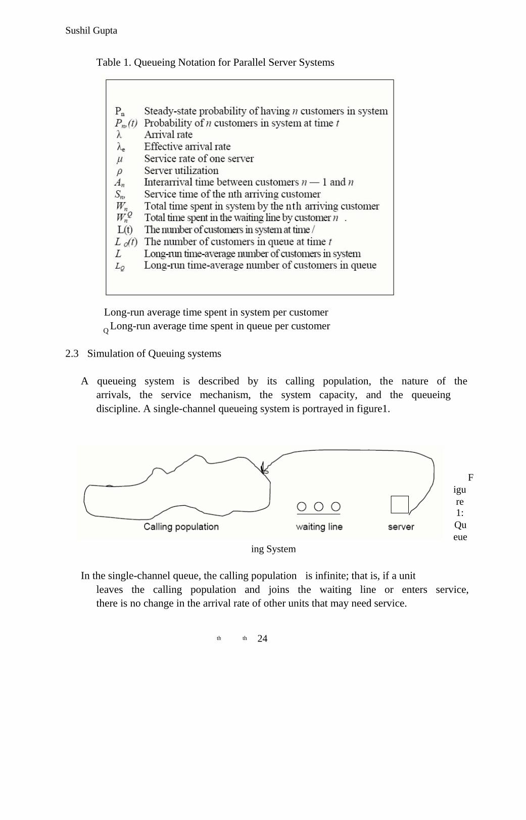
2.3 Simulation of Queuing systems
A queueing system is described by its calling population, the nature of the
arrivals, the service mechanism, the system capacity, and the queueing
discipline. A single-channel queueing system is portrayed in figure1.
F
igu
re
1:
Qu
eue
ing System
In the single-channel queue, the calling population is infinite; that is, if a unit
leaves the calling population and joins the waiting line or enters service,
there is no change in the arrival rate of other units that may need service.
24 th th
Sushil Gupta
Arrivals for service occur one at a time in a random fashion; once they join
the waiting line, they are eventu ally served. In addition, service times are of
some random length according to a probability distribution which does not
change over time.
The system capacity; has no limit, meaning that any number of units can
wait in line.
Finally, units are served in the order of their arrival by a single server or
channel.
Arrivals and services are defined by the distributions of the time between
arrivals and the distribution of service times, respectively.
For any simple sing le or multi-channel queue, the overall effective arrival
rate must be less than the total service rate, or the waiting line will grow
without bound. When queues grow without bound, they are termed
―explosive‖ or unstable.
The state of the system is the number of units in the system and the status of
the server, busy or idle.
An event is a set of circumstances that cause an instantaneous change in the
state of the system. In a single –channel queueing system there are only two
possible events that can affect the state of the system.
They are the entry of a unit into the system.
The co mpletion of service on a unit.
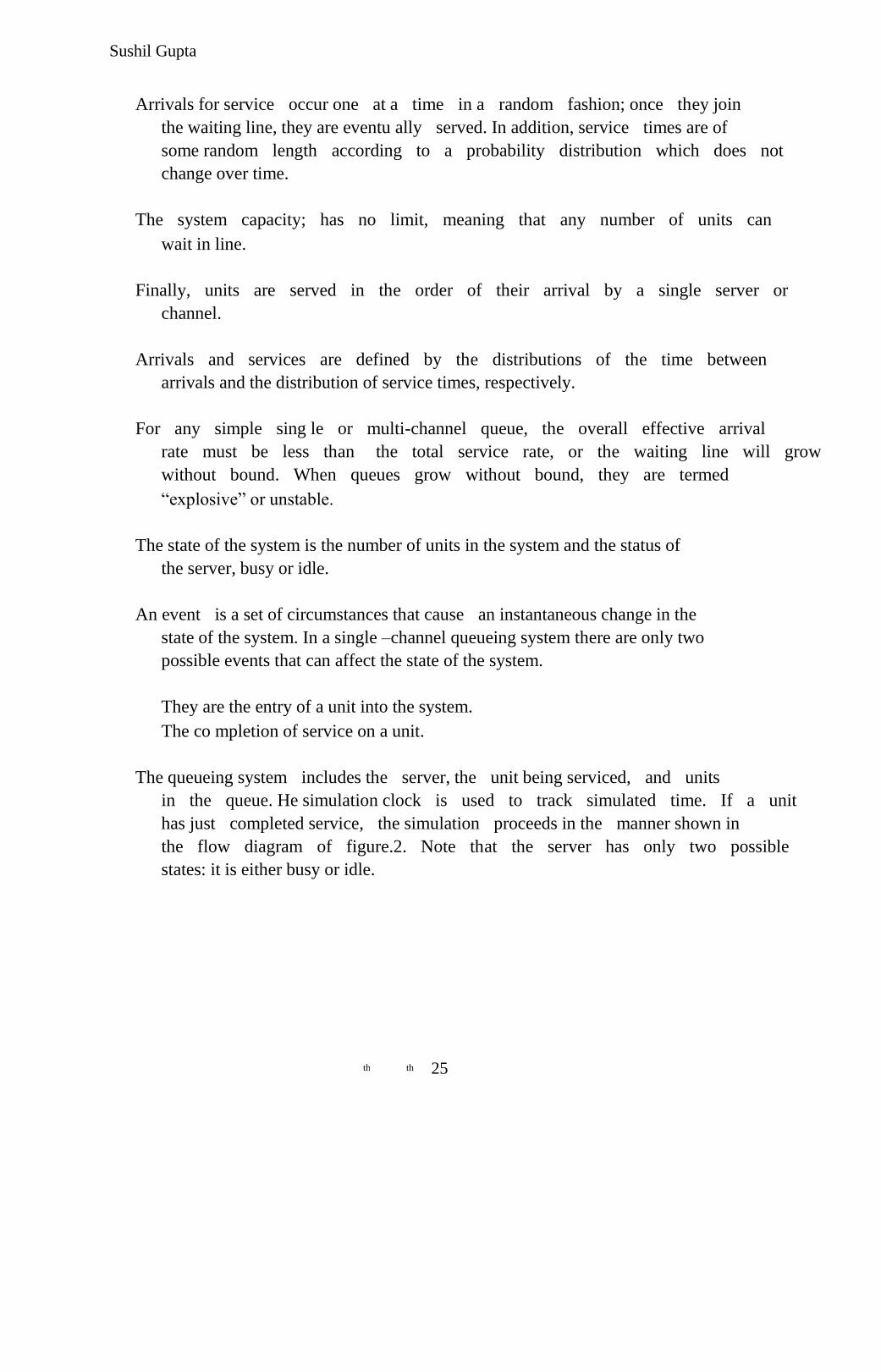
The queueing system includes the server, the unit being serviced, and units
in the queue. He simulation clock is used to track simulated time. If a unit
has just completed service, the simulation proceeds in the manner shown in
the flow diagram of figure.2. Note that the server has only two possible
states: it is either busy or idle.
25 th th
Sushil Gupta
Figure 2: Service-just-completed flow diagram
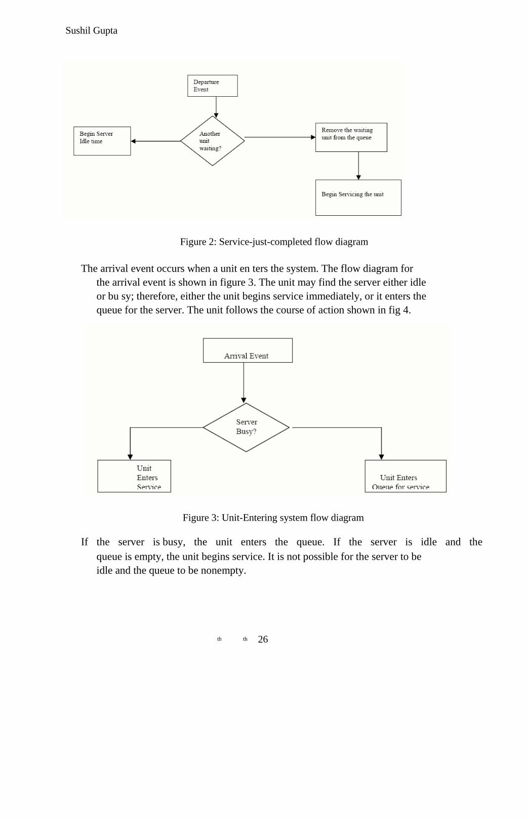
The arrival event occurs when a unit en ters the system. The flow diagram for
the arrival event is shown in figure 3. The unit may find the server either idle
or bu sy; therefore, either the unit begins service immediately, or it enters the
queue for the server. The unit follows the course of action shown in fig 4.
Figure 3: Unit-Entering system flow diagram
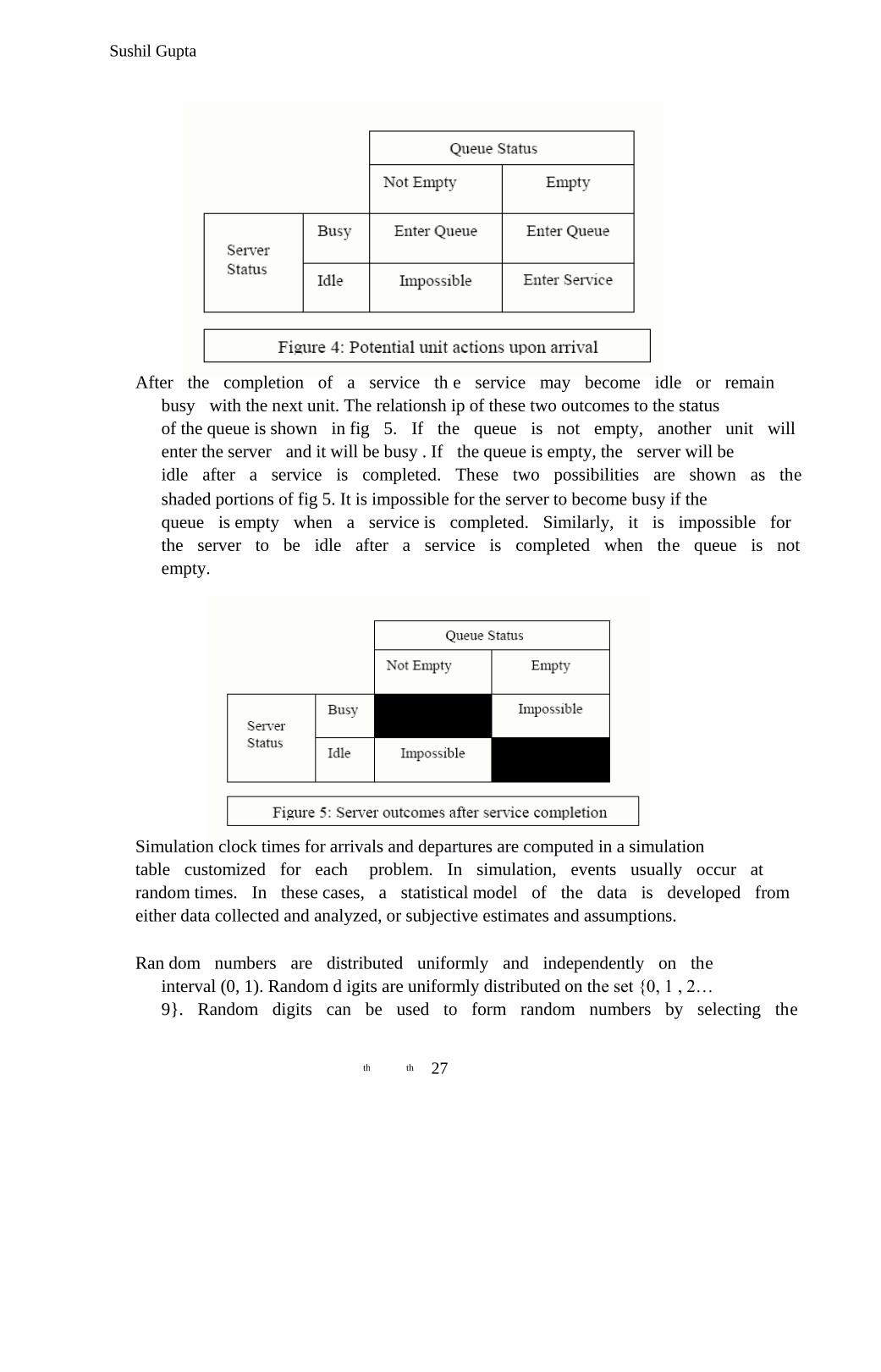
If the server is busy, the unit enters the queue. If the server is idle and the
queue is empty, the unit begins service. It is not possible for the server to be
idle and the queue to be nonempty.
26 th th
Sushil Gupta
After the completion of a service th e service may become idle or remain
busy with the next unit. The relationsh ip of these two outcomes to the status
of the queue is shown in fig 5. If the queue is not empty, another unit will
enter the server and it will be busy . If the queue is empty, the server will be
idle after a service is completed. These two possibilities are shown as the
shaded portions of fig 5. It is impossible for the server to become busy if the
queue is empty when a service is completed. Similarly, it is impossible for
the server to be idle after a service is completed when the queue is not
empty.
Simulation clock times for arrivals and departures are computed in a simulation
table customized for each problem. In simulation, events usually occur at
random times. In these cases, a statistical model of the data is developed from
either data collected and analyzed, or subjective estimates and assumptions.
Ran dom numbers are distributed uniformly and independently on the
interval (0, 1). Random d igits are uniformly distributed on the set {0, 1 , 2…
9}. Random digits can be used to form random numbers by selecting the
27 th th
Sushil Gupta
proper number of digits for each random number and placing a decimal
point to the left of the value selected. The proper number o f digits is dictated
by the accuracy of the data being used for input purposes. If the input
distribution has values with two decimal places, two digits are taken from a
random-digits table and the decimal point is placed to the left to form a
random number.
When numbers are generated using a procedure, they are often referred to as
pseudorandom numbers. Since the method is known, it is always possible to
know the sequence of numbers that will be generated prior to the simulation.
In a single-channel queuein g system, interarrival times and service times are
generated fro m the distributions of these random variables. The examples
that follow show how such times are generated. For simplicity, assume that
the times between arrivals were generated by rolling a die five times and
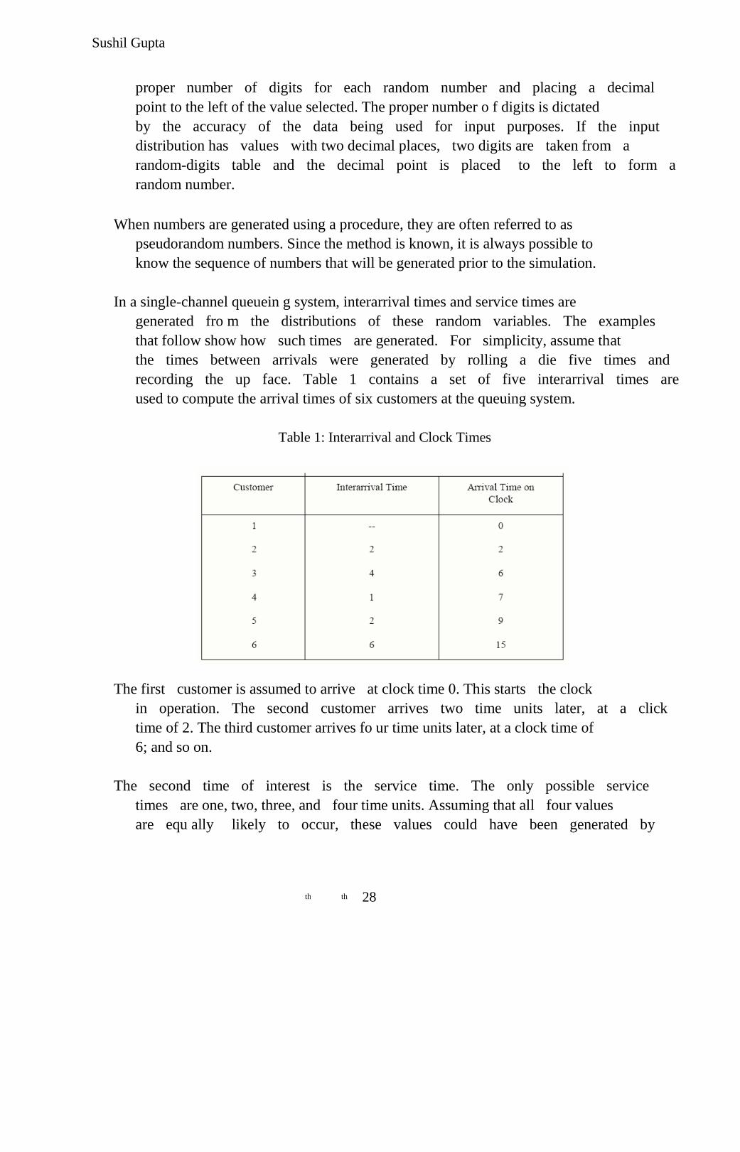
recording the up face. Table 1 contains a set of five interarrival times are
used to compute the arrival times of six customers at the queuing system.
Table 1: Interarrival and Clock Times
The first customer is assumed to arrive at clock time 0. This starts the clock
in operation. The second customer arrives two time units later, at a click
time of 2. The third customer arrives fo ur time units later, at a clock time of
6; and so on.
The second time of interest is the service time. The only possible service
times are one, two, three, and four time units. Assuming that all four values
are equ ally likely to occur, these values could have been generated by
28 th th
Sushil Gupta
placing the numbers one through four on chips and drawing the chips from a
hat with replacement, being sure to record the numbers selected.
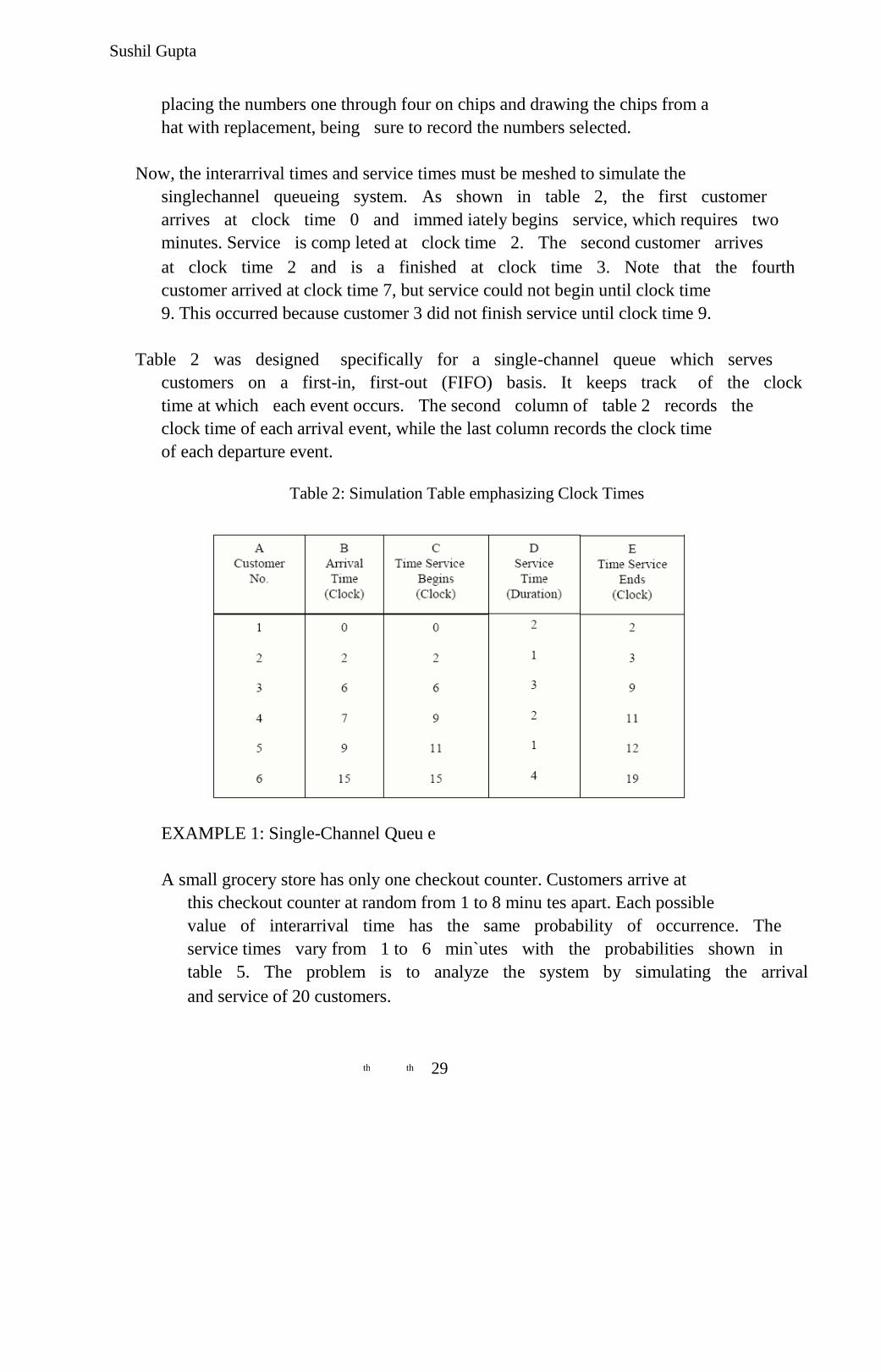
Now, the interarrival times and service times must be meshed to simulate the
singlechannel queueing system. As shown in table 2, the first customer
arrives at clock time 0 and immed iately begins service, which requires two
minutes. Service is comp leted at clock time 2. The second customer arrives
at clock time 2 and is a finished at clock time 3. Note that the fourth
customer arrived at clock time 7, but service could not begin until clock time
9. This occurred because customer 3 did not finish service until clock time 9.
Table 2 was designed specifically for a single-channel queue which serves
customers on a first-in, first-out (FIFO) basis. It keeps track of the clock
time at which each event occurs. The second column of table 2 records the
clock time of each arrival event, while the last column records the clock time
of each departure event.
Table 2: Simulation Table emphasizing Clock Times
EXAMPLE 1: Single-Channel Queu e
A small grocery store has only one checkout counter. Customers arrive at
this checkout counter at random from 1 to 8 minu tes apart. Each possible
value of interarrival time has the same probability of occurrence. The
service times vary from 1 to 6 min`utes with the probabilities shown in
table 5. The problem is to analyze the system by simulating the arrival
and service of 20 customers.
29 th th
Sushil Gupta
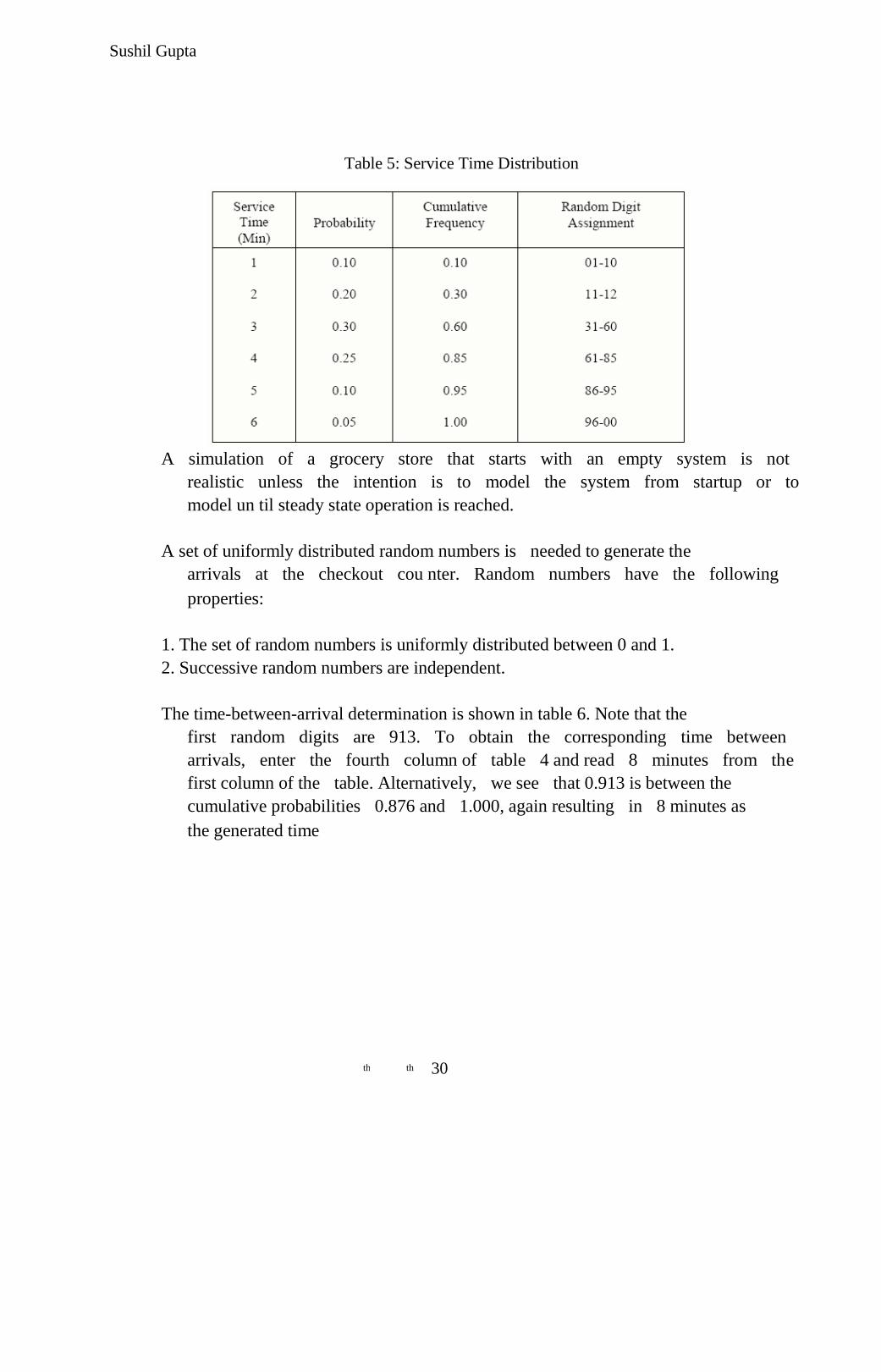
Table 5: Service Time Distribution
A simulation of a grocery store that starts with an empty system is not
realistic unless the intention is to model the system from startup or to
model un til steady state operation is reached.
A set of uniformly distributed random numbers is needed to generate the
arrivals at the checkout cou nter. Random numbers have the following
properties:
1. The set of random numbers is uniformly distributed between 0 and 1.
2. Successive random numbers are independent.
The time-between-arrival determination is shown in table 6. Note that the
first random digits are 913. To obtain the corresponding time between
arrivals, enter the fourth column of table 4 and read 8 minutes from the
first column of the table. Alternatively, we see that 0.913 is between the
cumulative probabilities 0.876 and 1.000, again resulting in 8 minutes as
the generated time
30 th th
Sushil Gupta
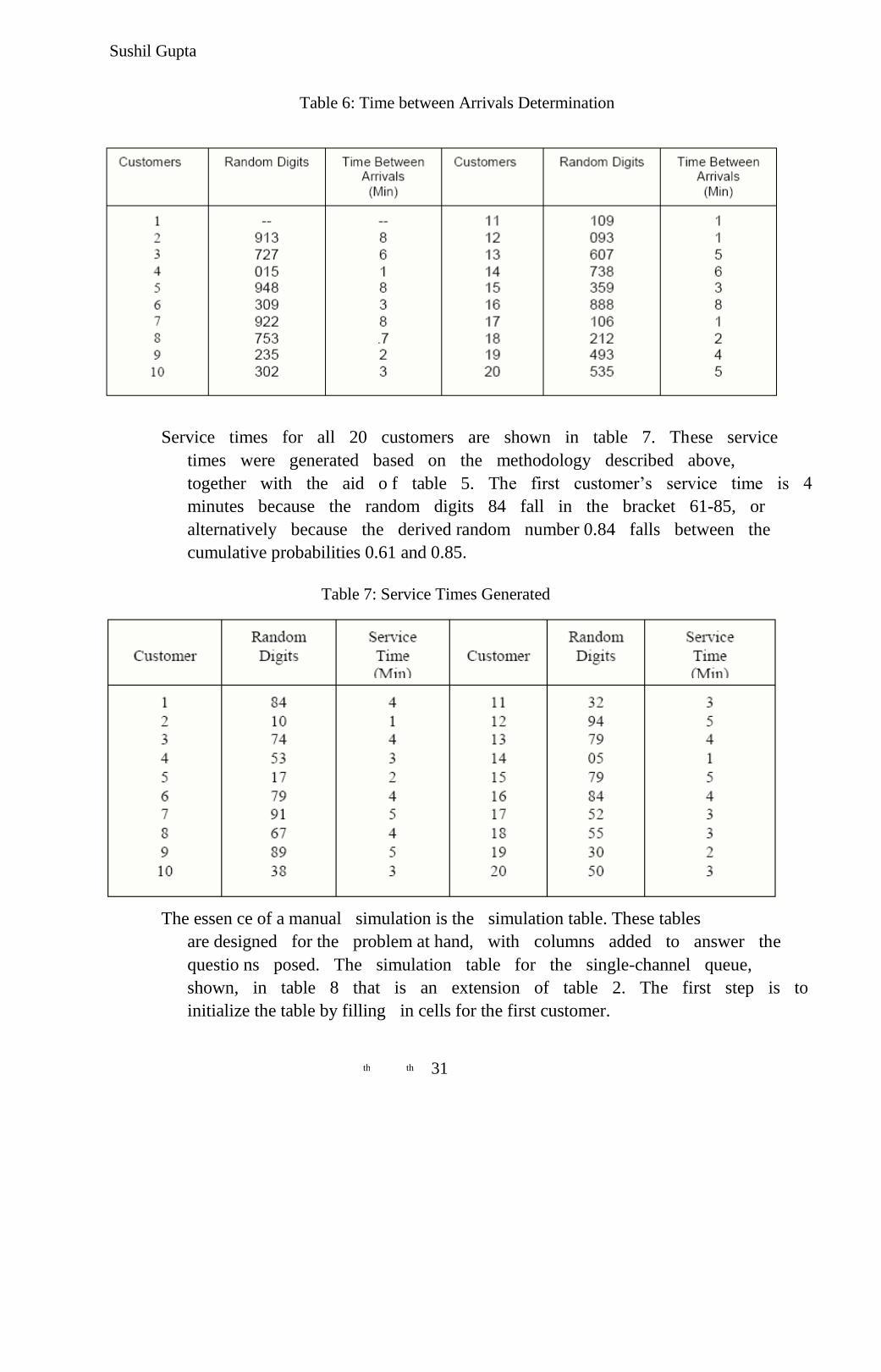
Table 6: Time between Arrivals Determination
Service times for all 20 customers are shown in table 7. These service
times were generated based on the methodology described above,
together with the aid o f table 5. The first customer‘s service time is 4
minutes because the random digits 84 fall in the bracket 61-85, or
alternatively because the derived random number 0.84 falls between the
cumulative probabilities 0.61 and 0.85.
Table 7: Service Times Generated
The essen ce of a manual simulation is the simulation table. These tables
are designed for the problem at hand, with columns added to answer the
questio ns posed. The simulation table for the single-channel queue,
shown, in table 8 that is an extension of table 2. The first step is to
initialize the table by filling in cells for the first customer.
31 th th
Sushil Gupta
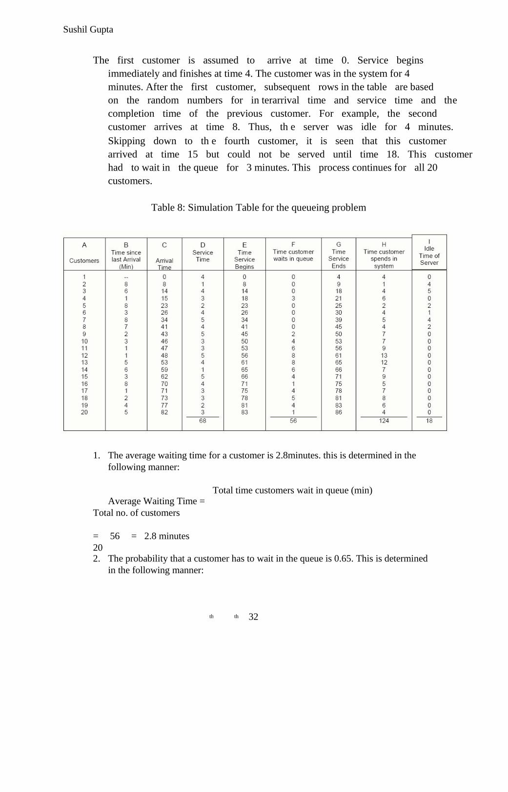
The first customer is assumed to arrive at time 0. Service begins
immediately and finishes at time 4. The customer was in the system for 4
minutes. After the first customer, subsequent rows in the table are based
on the random numbers for in terarrival time and service time and the
completion time of the previous customer. For example, the second
customer arrives at time 8. Thus, th e server was idle for 4 minutes.
Skipping down to th e fourth customer, it is seen that this customer
arrived at time 15 but could not be served until time 18. This customer
had to wait in the queue for 3 minutes. This process continues for all 20
customers.
Table 8: Simulation Table for the queueing problem
1. The average waiting time for a customer is 2.8minutes. this is determined in the
following manner:
Total time customers wait in queue (min)
Average Waiting Time =
Total no. of customers
= 56 = 2.8 minutes
20
2. The probability that a customer has to wait in the queue is 0.65. This is determined
in the following manner:
32 th th
Sushil Gupta
Probability (wait) = number of customers who wait
Total number of customers
13
= = 0.65
20
3. The fraction of idle time of the server is 0.21. This is determined in the
following manner:
Total idle time of server (minutes)
Probability of idle server =
Total run time of simulation (minutes)
18
= = 0.21
86
The probability of the server being busy is the complement of 0.21, or 0.79.
4. The average service time is 3.4 minutes, determined as follows:
Total service time
Average service time (minutes) =
Total number of customers
68
= = 3.4 minutes
20
This result can be compared with the expected service time by finding the mean
of the service-time distribution using the equation
E(s) = sp (s)
Applying the expected-value equation to the distribution in table 2.7 gives an
expected service time of:
= 1(0.10) + 2(0.20) + 3(0.30) + 4(0.25) + 5(0.10) + 6(0.50)
= 3.2 minutes
The expected service time is slightly lower than the aver age time in the
simulation. The longer simulation, the closer the average will be to E (S).
5. The average time between arrivals is 4.3 minutes. This is determined in the following
manner:
Sum of all times between arrivals (minutes)
Average time between arrivals (minutes) =
Number of arrivals - 1
82
33 th th
Sushil Gupta
= = 4.3 minutes
19
One is subtracted from the denominator because the first arrival is assumed to
occur at time 0. This result can be compared to the expected time between arrivals by
finding the mean of the discrete uniform distribution whose endpoints are a = 1 and b = 8.
The mean is given by
a + b 1 + 8
E (A) = = = 4.5 minutes
2 2
The expected time between arrivals is slightly higher than the average. However,
as the simulation becomes longer, the average value of the time between arrivals will approach the theoretical mean, E (A).
6. The average waiting time of those who wait is 4.3 minutes. This is determined in the
following manner:
Average waiting time of total time customers wait in queue
Those who wait (minutes) =
Total number of customers who wait
56
= = 4.3 minutes
13
7. The average time a customer spends in the system is 6.2 minutes. This can be
determined in two ways. First, the computation can be achieved by the following
relationship:
Average time customer total time customers spend in the system
Spends in the system =
Total number of customers
124
= = 6.2 minutes
20
The second way of computing this same result is to realize that the following relationship
must hold:
Average time customer average time customer average time customer
Spends in the system = spends waiting in the queue + spends in service
From findings 1 and 4 this results in:
Average time customer spends in the system = 2.8+ 3.4 = 6.2 minutes.
34 th th
Sushil Gupta
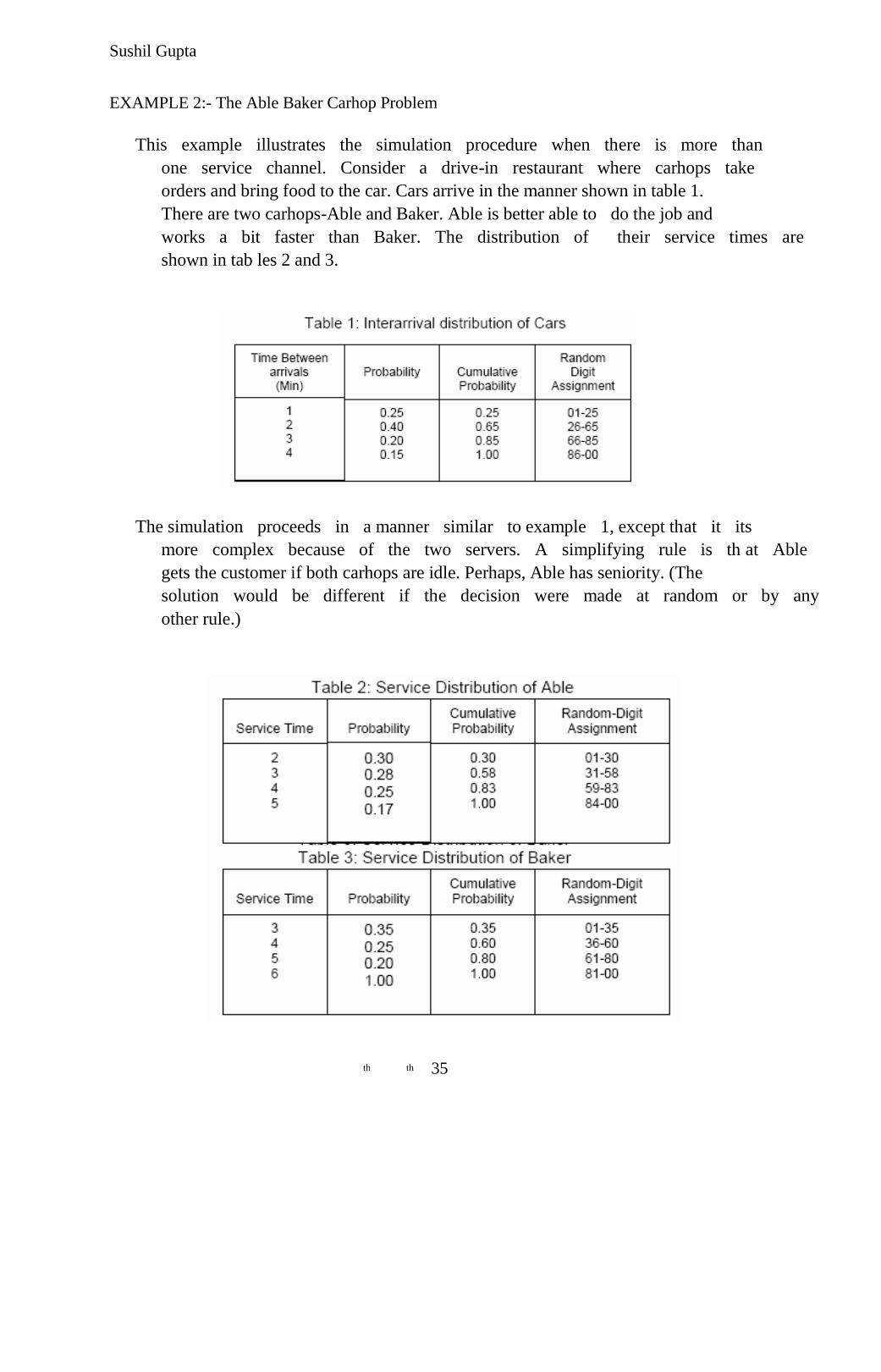
EXAMPLE 2:- The Able Baker Carhop Problem
This example illustrates the simulation procedure when there is more than
one service channel. Consider a drive-in restaurant where carhops take
orders and bring food to the car. Cars arrive in the manner shown in table 1.
There are two carhops-Able and Baker. Able is better able to do the job and
works a bit faster than Baker. The distribution of their service times are
shown in tab les 2 and 3.
The simulation proceeds in a manner similar to example 1, except that it its
more complex because of the two servers. A simplifying rule is th at Able
gets the customer if both carhops are idle. Perhaps, Able has seniority. (The
solution would be different if the decision were made at random or by any
other rule.)
35 th th

Sushil Gupta
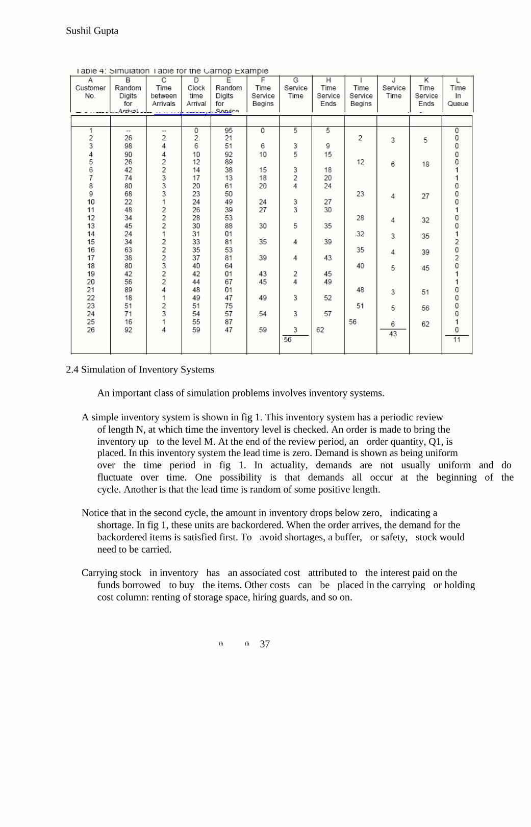
Here there are more events: a customer arrives, a customer begins ser vice from able, a
customer completes service from Able, a customer begins service from Baker, and a
customer completes service from Baker. The simulation table is shown in table 4.
After the first customer, the cells for the other customers must be based on logic and
formulas. For example, the ―clock time of arrival‖ in the row for the second customer is
computed as follows: D2 = D1+C2
The logic to compute who gets a given customer, and when that service begins, is more
complex. The logic goes as follows when a customer arrives: if the customer finds able
idle, the customer begins service immediately with able. If able is not idle but baker is, then the customer begins service immediately with baker. If both are busy, the customer
begins service with the first server to become free.
The analysis of table 4 results in the following:
1. Over the 62-minute period able was busy 90% of the time.
2. Baker was busy only 69% of the tome. The seniority rule keeps baker less busy.
3. Nine of the 26 arrivals had to wait. The average waiting time for all customer s was
only about 0.42 minute, which is very small.
4. Those nine who did have to wait only waited an average of 1.22 minutes, which is
quite low.
5. In summary, this system seems well balanced. One server cannot handle all the diners,
and three servers would probably be too many. Adding an additional server would
surely reduce the waiting time to nearly zero. However, the cost of waiting would have
to be quite high to justify an additional server.
Table 4: Simulation Table for the Carhop Exam ple
36 th th
Sushil Gupta
2.4 Simulation of Inventory Systems
An important class of simulation problems involves inventory systems.
A simple inventory system is shown in fig 1. This inventory system has a periodic review
of length N, at which time the inventory level is checked. An order is made to bring the
inventory up to the level M. At the end of the review period, an order quantity, Q1, is
placed. In this inventory system the lead time is zero. Demand is shown as being uniform
over the time period in fig 1. In actuality, demands are not usually uniform and do
fluctuate over time. One possibility is that demands all occur at the beginning of the
cycle. Another is that the lead time is random of some positive length.
Notice that in the second cycle, the amount in inventory drops below zero, indicating a
shortage. In fig 1, these units are backordered. When the order arrives, the demand for the
backordered items is satisfied first. To avoid shortages, a buffer, or safety, stock would
need to be carried.
Carrying stock in inventory has an associated cost attributed to the interest paid on the
funds borrowed to buy the items. Other costs can be placed in the carrying or holding
cost column: renting of storage space, hiring guards, and so on.
37 th th
Sushil Gupta
An alternative to carrying high inventory is to make more frequent reviews, and
consequently, more frequent purchases or replenishments. This has an associated cost:
the ordering cost. Also, there is a cost in being short. Larger inventories decrease the
possibilities of shortages. These costs must be traded off in order to minimize the total
cost of an inventory system.
The total cost of an inventory system is the measure of performance. This can be affected
by the policy alternatives. For example, in fig 1, the decision maker can control the
maximum inventory level, M, and the cycle, N.
In an (M, N) inventory system, the events that may occur are: the demand for items in the
inventory, the review of the inventory position, and the receipt of an order at the end of
each review period. When the lead time is zero, as in fig 1, the last two events occur
simultaneously.
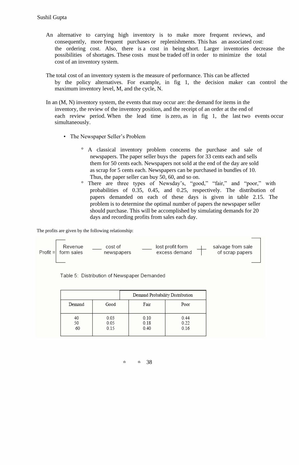
• The Newspaper Seller‘s Problem
° A classical inventory problem concerns the purchase and sale of
newspapers. The paper seller buys the papers for 33 cents each and sells
them for 50 cents each. Newspapers not sold at the end of the day are sold
as scrap for 5 cents each. Newspapers can be purchased in bundles of 10.
Thus, the paper seller can buy 50, 60, and so on. ° There are three types of Newsday‘s, ―good,‖ ―fair,‖ and ―poor,‖ with
probabilities of 0.35, 0.45, and 0.25, respectively. The distribution of
papers demanded on each of these days is given in table 2.15. The
problem is to determine the optimal number of papers the newspaper seller
should purchase. This will be accomplished by simulating demands for 20
days and recording profits from sales each day.
The profits are given by the following relationship:
38 th th
Sushil Gupta
° Form the problem statement, the revenue from sales is 50 cents for each
paper sold. The Cost 9 of newspapers is 33 cents for each paper
purchased. The lost profit from excess demand is 17 cents for each paper
demanded that could not be provided. Such a shortage cost is somewhat
controversial but makes the problem much more interesting. The salvage
value of scrap papers is 5 cents each.
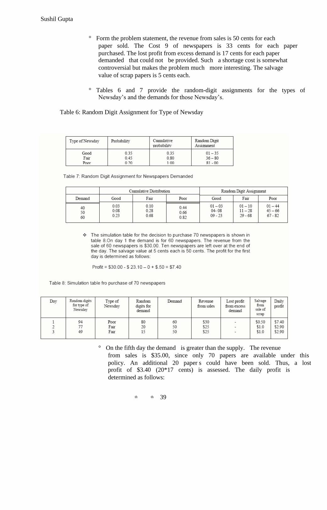
° Tables 6 and 7 provide the random-digit assignments for the types of
Newsday‘s and the demands for those Newsday‘s.
Table 6: Random Digit Assignment for Type of Newsday
° On the fifth day the demand is greater than the supply. The revenue
from sales is $35.00, since only 70 papers are available under this
policy. An additional 20 paper s could have been sold. Thus, a lost profit of $3.40 (20*17 cents) is assessed. The daily profit is
determined as follows:
39 th th
Sushil Gupta
Profit = $35.00 - $23.10 - $3.40 + 0 = $8.50
° The profit for the 20-day period is the sum of the daily profits,
$174.90. it can also be computed from the totals for the 20 days of the
simulation as follows:
Total profit = $645 - $462 - $13 .60 + $5.50 = $174.90
° In general, since the results of one day are independent of those of
previous days, inventory problems of this type are easier than
queueing problems.
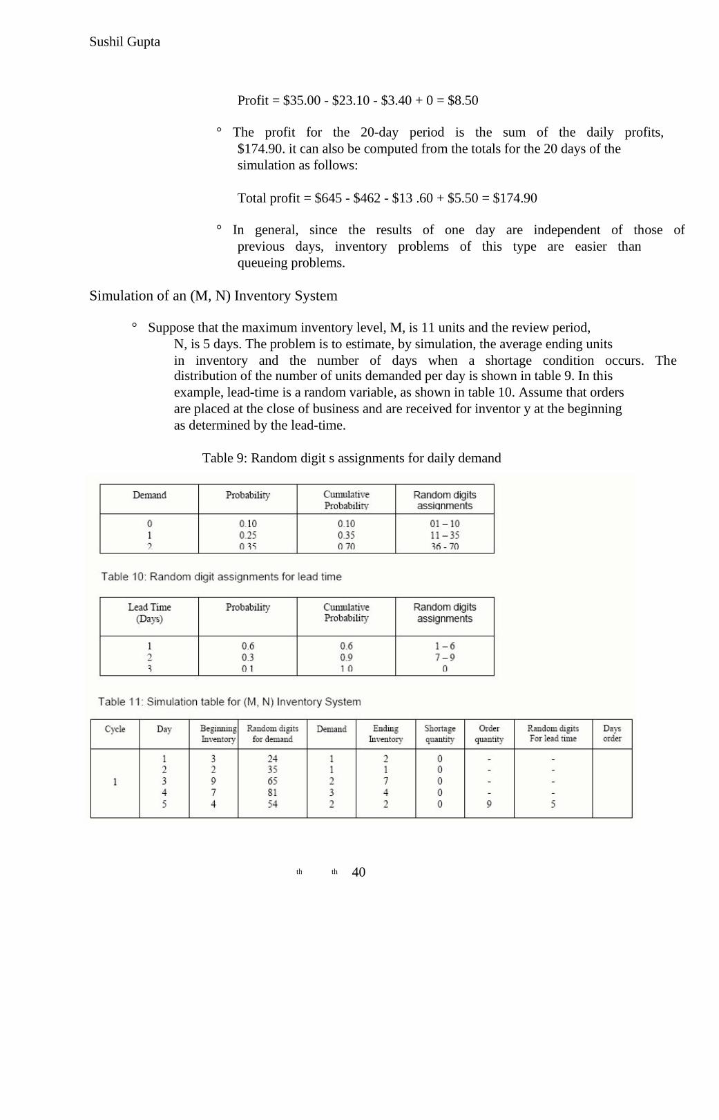
Simulation of an (M, N) Inventory System
° Suppose that the maximum inventory level, M, is 11 units and the review period,
N, is 5 days. The problem is to estimate, by simulation, the average ending units
in inventory and the number of days when a shortage condition occurs. The
distribution of the number of units demanded per day is shown in table 9. In this
example, lead-time is a random variable, as shown in table 10. Assume that orders
are placed at the close of business and are received for inventor y at the beginning
as determined by the lead-time.
Table 9: Random digit s assignments for daily demand
40 th th

Sushil Gupta
Note : Refer cycle 2,3,4,5 from Text book page no 47.
To make an estimate of the mean units in ending inventory, many cycles would
have to be simulated. For purposes of this example, only five cycles will be
shown. The reader is asked to continue the example as an exercise at the end of
the chapter.
The random-digit assignments for daily demand and lead time are shown in the
rightmost columns of tables 9 and 10. The resulting simulation table is shown in
table 11.The simulation has been started with the inventory level at 3 units and an
order of 8 units scheduled to arrive in 2 days time.
Following the simulation table for several selected days indicates how the process
operates. The order for 8 units is available on the morning of the third day of the
first cycle, raising the inventory level from 1 unit to 9 units; demands during the
remainder of the first cycle reduced the ending inventory level to 2 units on the
fifth day. Thus, an order for 9 units was placed. The lead time for this order was 1
day. The order of 9 units was added to inventory on the morning of day 2 of cycle
2.
Notice that the beginning inventory on the second day of the third cycle was zero.
An order for 2 units on that day led to a shortage condition. The units were
backordered on that day and the next day;; also on the morning of day 4 of cycle 3
there was a beginning inventory of 9 units that were backordered and the 1 unit
demanded that day reduced the ending inventory to 4 units.
Based on five cycles of simulation, the average ending inventory is approximately
3.5 (88/25) units. On 2 of 25 days a shortage condition existed.
41 th th
Sushil Gupta
CHAPTER - 3
GENERAL PRINCIPLES
Introduction
• This chapter develops a common framework for the modeling of complex systems
using discrete-event simulation.
• It covers the basic building blocks of all discrete-event simulation models: entities
and attributes, activities and events.
• In discrete-event simulation, a system is modeled in terms of its state at each point in
time; the entities that pass through the system and the entities that rep-j resent system
resources; and the activities and events that cause system state to change.
• This chapter deals exclusively with dynamic, stochastic system (i.e. involving time
and containing random elements) which changes in a discrete manner.
3.1 Concepts in Discrete-Event Simulation
• The concept of a system and a model of a system were discussed briefly in earlier
chapters.
• This section expands on these concepts and develops a framework for the
development of a discrete-event model of a system.
• The major concepts are briefly defined and then illustrated with examples:
• System: A collection of entities ( e.g., people and machines) that ii together over
time to accomplish one or more goals.
• Model: An abstract representation of a system, usually containing structural, logical, or mathematical relationships which describe a system in terms of state,
entities and their attributes, sets, processes, events, activities, and delays.
• System state: A collection of variables that contain all the information necessary
to describe the system at any time.
42 th th
Sushil Gupta
• Entity: Any object or component in the system which requires explicit
representation in the model (e.g., a server, a customer, a machine).
• Attributes: The properties of a given entity (e.g., the priority of a v customer, the
routing of a job through a job shop).
• List: A collection of (permanently or temporarily) associated entities ordered in
some logical fashion (such as all customers currently in a waiting line, ordered by
first come, first served, or by priority).
• Event: An instantaneous occurrence that changes the state of a system as an
arrival of a new customer).
• Event notice: A record of an event to occur at the current or some future time,
along with any associated data necessary to execute the event; at a minimum, the
record includes the event type and the event time.
• Event list: A list of event notices for future events, ordered by time of occurrence;
also known as the future event list (FEL).
• Activity: A duration of time of specified length (e.g., a service time or arrival
time), which is known when it begins (although it may be defined in terms of a
statistical distribution).
• Delay: A duration of time of unspecified indefinite length, which is not known
until it ends (e.g., a customer's delay in a last-in, first-out waiting line which,
when it begins, depends on future arrivals).
• Clock: A variable representing simulated time. · The future event list is ranked by
the event time recorded in the event notice.
An activity typically represents a service time, an interarrival time, or any other
processing time whose duration has been characterized and defined by the modeler.
An activity‘s duration may be specified in a number of ways:
1. Deterministic-for example, always exactly 5 minutes.
2. Statistical-for example, as a random draw from among 2,5,7 with equal probabilities. 3. A function depending on system variables and/or entity attributes.
The duration of an activity is computable from its specification at the instant it begins.
A delay's duration is not specified by the modeler ahead of time, but rather is
determined by system conditions.
A delay is sometimes called a conditional wait, while an activity is called unconditional
wait.
43 th th
Sushil Gupta
The completion of an activity is an event, often called primary event.
The completion of a delay is sometimes called a conditional or secondary event.
EXAMPLE 3.1 (Able and Baker, Revisited)
Consider the Able-Baker carhop system of Example 2.2. A discr ete- event model has the
following components:
System State
LQ(t), the number of cars waiting to be served at time t
LA(t), 0 or 1 to indicate Able being idle or busy at time t
LB (t), 0 or 1 to indicate Baker being idle or busy at time t
Entities
Neither the customers (i.e., cars) nor the servers need to be explicitly represented, except
in terms of the state variables, unless certain customer averages are desired (compare Examples
3.4 and 3.5)
Events
Arrival event Service completion by Able
Service completion by Baker
Activities
Interarrival time, defined in Table 2.11
Service time by Able, defined in Table 2.12
Service time by Baker, defined in Table 2.13
Delay
A customer's wait in queue until Able or Baker becomes free.
3.2 The Event-Scheduling/Time-Advance Algorithm
The mechanism for advancing simulation time and guaranteeing that all events occur in
correct chronological order is based on the future event list (FEL).
This list contains all event notices for events that have been scheduled to occur at a future
time.
44 th th
Sushil Gupta
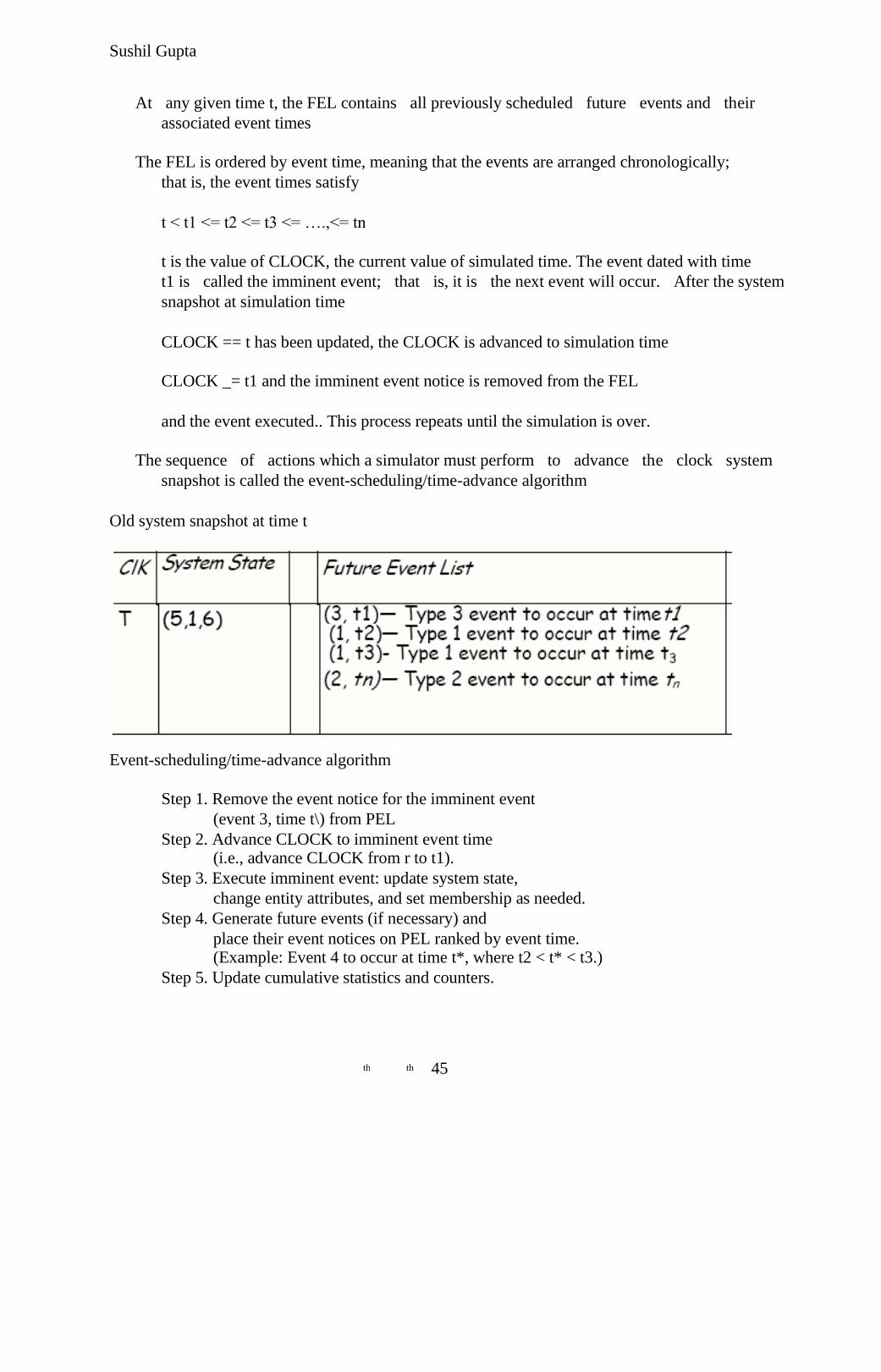
At any given time t, the FEL contains all previously scheduled future events and their
associated event times
The FEL is ordered by event time, meaning that the events are arranged chronologically;
that is, the event times satisfy
t < t1 <= t2 <= t3 <= ….,<= tn
t is the value of CLOCK, the current value of simulated time. The event dated with time
t1 is called the imminent event; that is, it is the next event will occur. After the system
snapshot at simulation time
CLOCK == t has been updated, the CLOCK is advanced to simulation time
CLOCK _= t1 and the imminent event notice is removed from the FEL
and the event executed.. This process repeats until the simulation is over.
The sequence of actions which a simulator must perform to advance the clock system
snapshot is called the event-scheduling/time-advance algorithm
Old system snapshot at time t
Event-scheduling/time-advance algorithm
Step 1. Remove the event notice for the imminent event
(event 3, time t\) from PEL
Step 2. Advance CLOCK to imminent event time
(i.e., advance CLOCK from r to t1).
Step 3. Execute imminent event: update system state,
change entity attributes, and set membership as needed.
Step 4. Generate future events (if necessary) and
place their event notices on PEL ranked by event time. (Example: Event 4 to occur at time t*, where t2 < t* < t3.)
Step 5. Update cumulative statistics and counters.
45 th th
Sushil Gupta
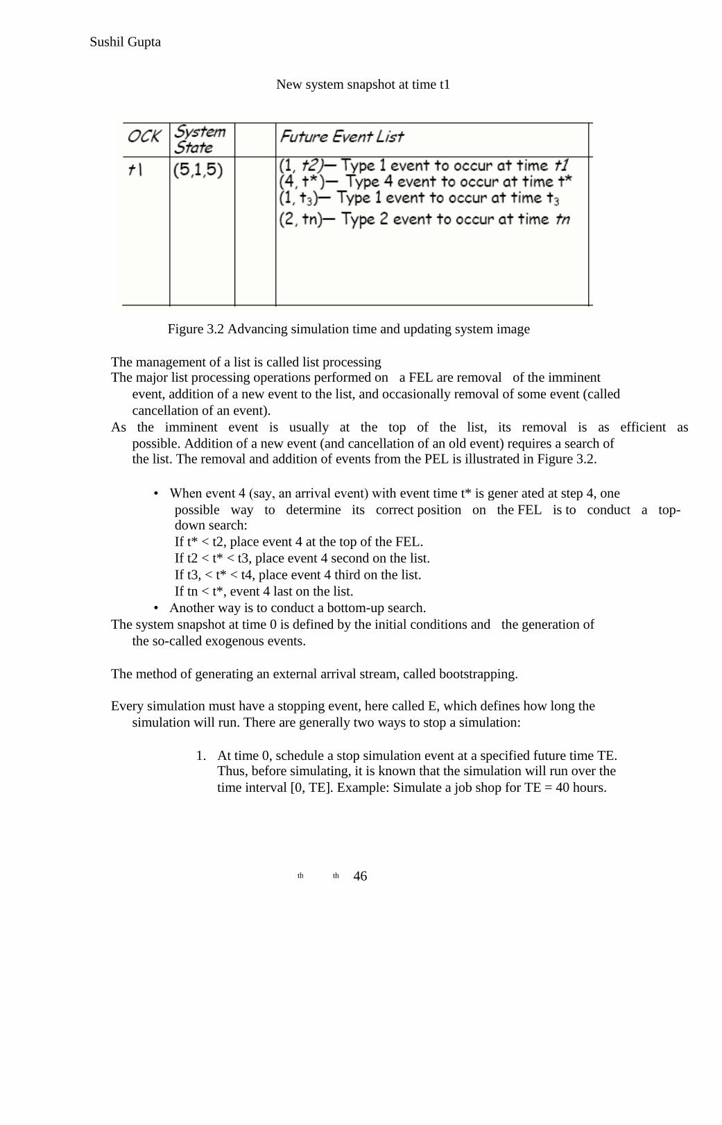
New system snapshot at time t1
Figure 3.2 Advancing simulation time and updating system image
The management of a list is called list processing
The major list processing operations performed on a FEL are removal of the imminent
event, addition of a new event to the list, and occasionally removal of some event (called
cancellation of an event).
As the imminent event is usually at the top of the list, its removal is as efficient as
possible. Addition of a new event (and cancellation of an old event) requires a search of
the list. The removal and addition of events from the PEL is illustrated in Figure 3.2.
• When event 4 (say, an arrival event) with event time t* is gener ated at step 4, one
possible way to determine its correct position on the FEL is to conduct a top-
down search:
If t* < t2, place event 4 at the top of the FEL.
If t2 < t* < t3, place event 4 second on the list.
If t3, < t* < t4, place event 4 third on the list.
If tn < t*, event 4 last on the list.
• Another way is to conduct a bottom-up search.
The system snapshot at time 0 is defined by the initial conditions and the generation of
the so-called exogenous events.
The method of generating an external arrival stream, called bootstrapping.
Every simulation must have a stopping event, here called E, which defines how long the
simulation will run. There are generally two ways to stop a simulation:
1. At time 0, schedule a stop simulation event at a specified future time TE. Thus, before simulating, it is known that the simulation will run over the
time interval [0, TE]. Example: Simulate a job shop for TE = 40 hours.
46 th th
Sushil Gupta
2. Run length TE is determined by the simulation itself. Generally, TE is the
time of occurrence of some specified event E. Examples: TE is the time of
the 100th service completion at a certain service center. TE is the time of
breakdown of a complex system.
3.3 World Views
• When using a simulation package or even when using a manual simulation, a
modeler adopts a world view or orientation for developing a model.
• Those most prevalent are the event scheduling world view, the process-interaction
worldview, and the activity-scanning world view.
• When using a package that supports the process-interaction approach, a
simulation analyst thinks in terms of processes .
• When using the event-scheduling approach, a simulation analyst concentrates on
events and their effect on system state.
• The process-interaction approach is popular because of its intuitive appeal, and
because the simulation packages that implement it allow an analyst to describe the
process flow in terms of high-level block or network constructs.
• Both the event-scheduling and the process-interaction approaches use a / variable
time advance.
• The activity- scanning approach uses a fixed time increment and a rule-based
approach to decide whether any activities can begin at each point in simulated
time.
• The pure activity scanning approach has been modified by what is called the
three-phase approach.
• In the three-phase approach, events are considered to be activity duration-zero
time units. With this definition, activities are divided into two categories called B
and C.
V B activities: Activities bound to occur; all primary
V C activities: Activities or events that are conditional upon certain
conditions being true.
• With the. three-phase approach the simulation proceeds with repeated execution
of the three phases until it is completed:
‹ Phase A: Remove the imminent event from the FEL and advance the clock
to its event time. Remove any other events from the FEL that have the
event time.
‹ Phase B: Execute all B-type events that were removed from the FEL.
‹ Phase C: Scan the conditions that trigger each C-type activity and activate
any whose conditions are met. Rescan until no additional C-type activities
can begin or events occur.
47 th th
Sushil Gupta
• The three-phase approach improves the execution efficiency of the activity
scanning method.
EXAMPLE 3.2 (Able and Baker, Back Again)
Using the three-phase approach, the conditions for beginning each activity in Phase C are:
Activity Condition
Service time by Able A customer is in queue and Able is idle,
Service time by Baker A customer is in queue, Baker is idle,
and Able is busy.
3.4 Manual Simulation Using Event Scheduling
• In an event-scheduling simulation, a simulation table is used to record the
successive system snapshots as time advances.
• Lets consider the example of a grocery shop which has only one checkout counter.
Example 3.3 (Single-Channel Queue)
• The system consists of those customers in the waiting line plus the one (if any)
checking out.
• The model has the following components:
System state ‹ (LQ(i), Z,S(r)), where LQ((] is the number of customers in the
waiting line, and LS(t) is the number being served (0 or 1) at time t.
Entities ‹ The server and customers are not explicitly modeled, except in
terms of the state variables above.
‹ Events
Arrival (A)
Departure (D)
Stopping event (£"), scheduled to occur at time 60.
‹ Event notices
(A, i). Representing an arrival event to occur at future time t
(D, t), representing a customer departure at future time t
(£, 60), representing the simulation-stop event at future time 60
‹ Activities
Inlerarrival time, denned in Table 2.6
Service time, defined in Table 2.7
48 th th
Sushil Gupta
‹ Delay
Customer time spent in waiting line.
• In this model, the FEL will always contain either two or three event notices.
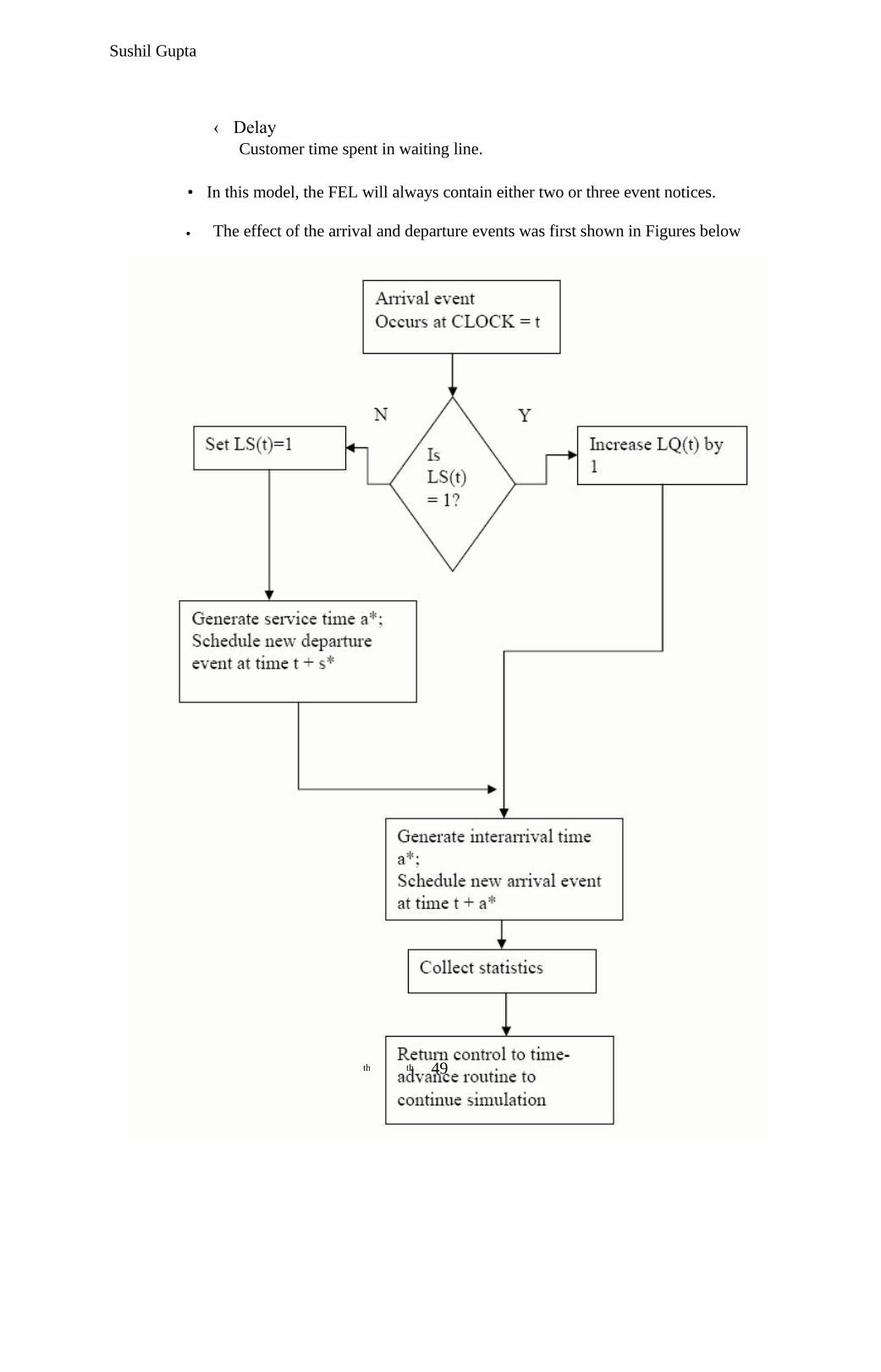
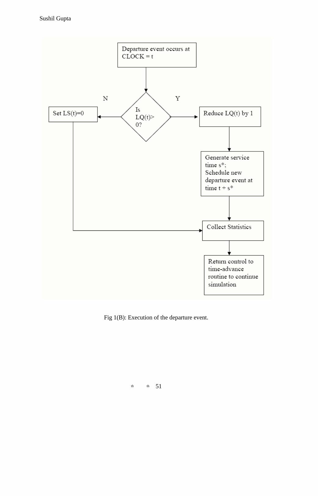
The effect of the arrival and departure events was first shown in Figures below •
49 th th

Sushil Gupta
Fig 1(A): Execution of the arrival event.
50 th th
Sushil Gupta
Fig 1(B): Execution of the departure event.
51 th th
Sushil Gupta
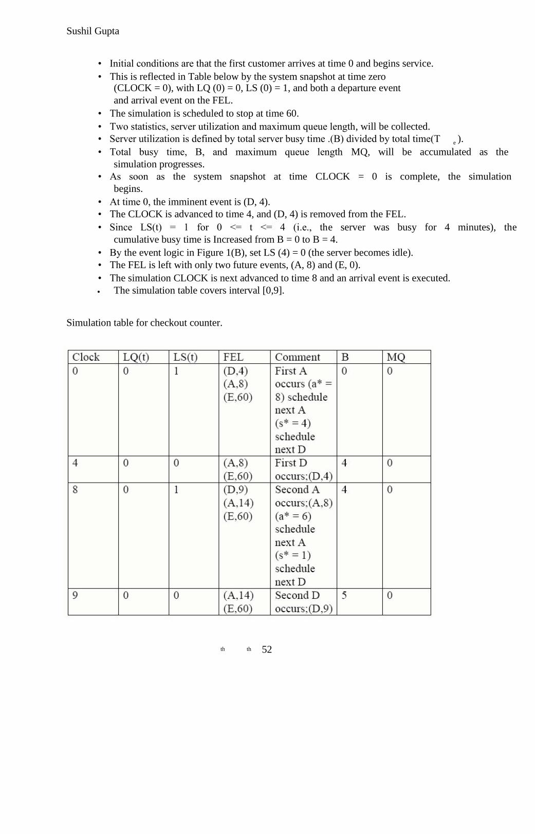
• Initial conditions are that the first customer arrives at time 0 and begins service.
• This is reflected in Table below by the system snapshot at time zero
(CLOCK = 0), with LQ (0) = 0, LS (0) = 1, and both a departure event
and arrival event on the FEL.
• The simulation is scheduled to stop at time 60.
• Two statistics, server utilization and maximum queue length, will be collected.
• Server utilization is defined by total server busy time .(B) divided by total time(T ). e
• Total busy time, B, and maximum queue length MQ, will be accumulated as the
simulation progresses.
• As soon as the system snapshot at time CLOCK = 0 is complete, the simulation
begins.
• At time 0, the imminent event is (D, 4).
• The CLOCK is advanced to time 4, and (D, 4) is removed from the FEL.
• Since LS(t) = 1 for 0 <= t <= 4 (i.e., the server was busy for 4 minutes), the
cumulative busy time is Increased from B = 0 to B = 4.
• By the event logic in Figure 1(B), set LS (4) = 0 (the server becomes idle).
• The FEL is left with only two future events, (A, 8) and (E, 0).
• The simulation CLOCK is next advanced to time 8 and an arrival event is executed.
The simulation table covers interval [0,9]. •
Simulation table for checkout counter.
52 th th
Sushil Gupta
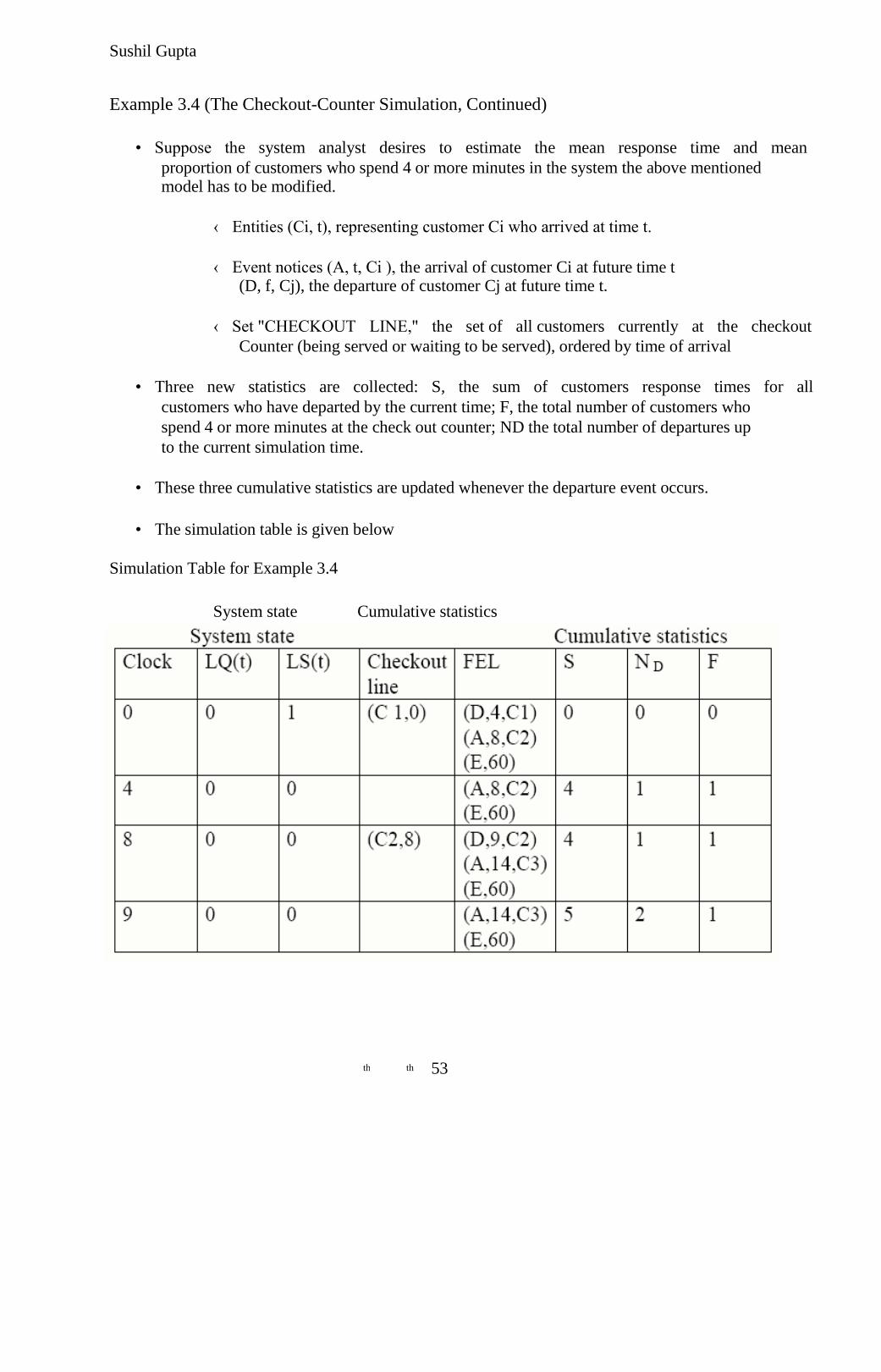
Example 3.4 (The Checkout-Counter Simulation, Continued)
• Suppose the system analyst desires to estimate the mean response time and mean
proportion of customers who spend 4 or more minutes in the system the above mentioned
model has to be modified.
‹ Entities (Ci, t), representing customer Ci who arrived at time t.
‹ Event notices (A, t, Ci ), the arrival of customer Ci at future time t (D, f, Cj), the departure of customer Cj at future time t.
‹ Set "CHECKOUT LINE," the set of all customers currently at the checkout
Counter (being served or waiting to be served), ordered by time of arrival
• Three new statistics are collected: S, the sum of customers response times for all
customers who have departed by the current time; F, the total number of customers who
spend 4 or more minutes at the check out counter; ND the total number of departures up
to the current simulation time.
• These three cumulative statistics are updated whenever the departure event occurs.
• The simulation table is given below
Simulation Table for Example 3.4
System state Cumulative statistics
53 th th
Sushil Gupta
Example 3.5 (The Dump Truck Problem)
• Six dump truck are used to haul coal from the entrance of a small mine to the railroad.
• Each truck is loaded by one of two loaders.
• After loading, a truck immediately moves to scale, to be weighted as soon as possible.
• Both the loaders and the scale have a first come, first serve waiting line(or queue) for
trucks.
• The time taken to travel from loader to scale is considered negligible.
• After being weighted, a truck begins a travel time and then afterward returns to the loader
queue.
• The model has the following components:
‹ System state
[LQ(0, L(f), WQ(r), W(r)], where
LQ(f) = number of trucks in loader queue
L(t) = number of trucks (0,1, or 2)being Loaded
WQ(t)= number of trucks in weigh queue
W(t) = number of trucks (0 or 1) being weighed, all at simulation time t
‹ Event notices
(ALQ,, t, DTi), dump truck arrives at loader queue
(ALQ) at time t (EL, t, DTi), dump truck i ends loading (EL) at time t
(EW, t, DTi), dump truck i ends weighing (EW) at time t
‹ Entities The six dump trucks (DTI,..., DT6)
‹ Lists
Loader queue, all trucks waiting to begin loading,
ordered on a first-come, first-served basis
Weigh queue, all trucks waiting to be weighed, ordered
on a first-come, first-serve basis.
‹ Activities Loading time, weighing time, and travel time.
‹ Delays Delay at loader queue, and delay at scale.
54 th th
Sushil Gupta
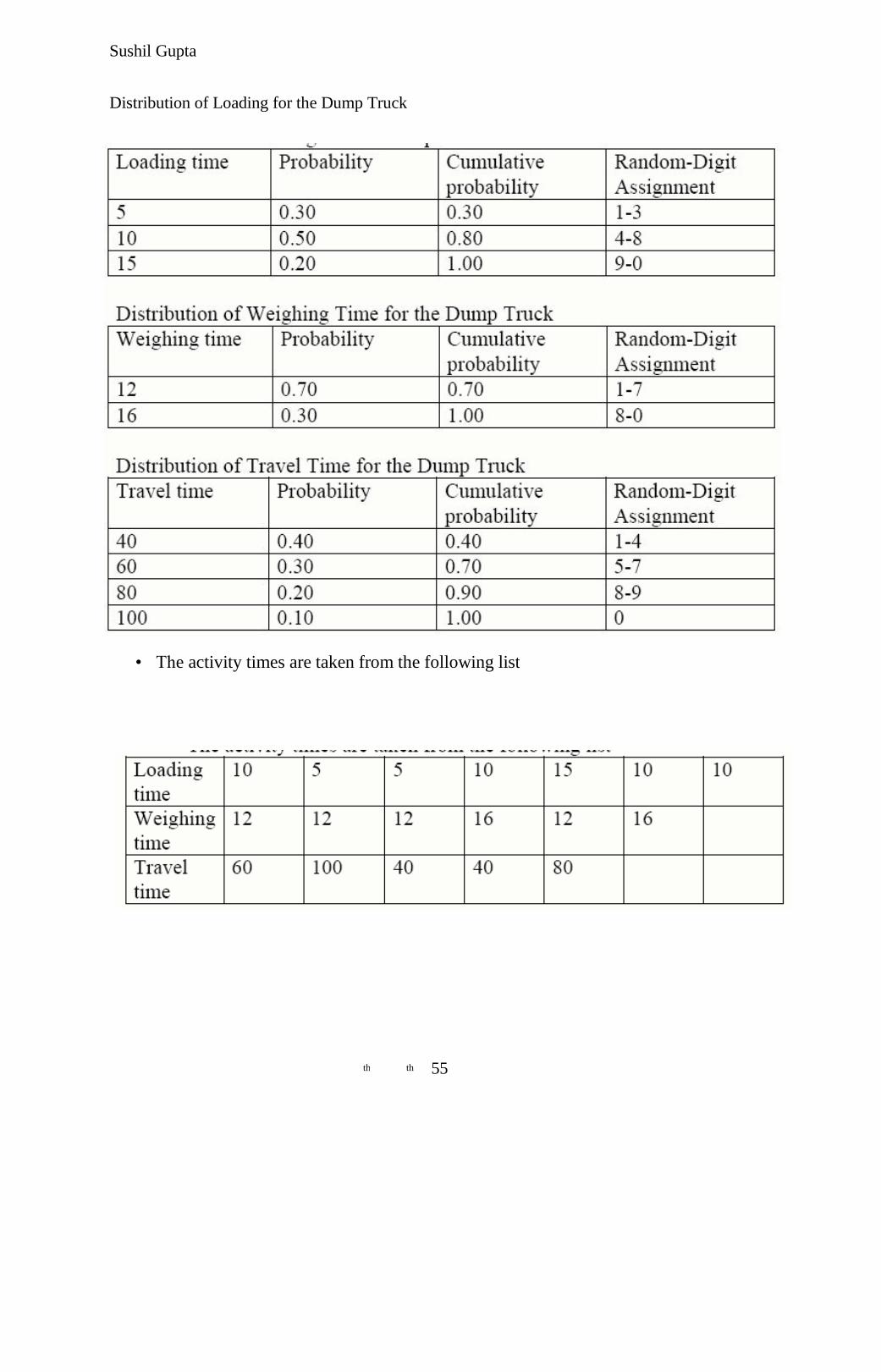
Distribution of Loading for the Dump Truck
• The activity times are taken from the following list
55 th th
Sushil Gupta
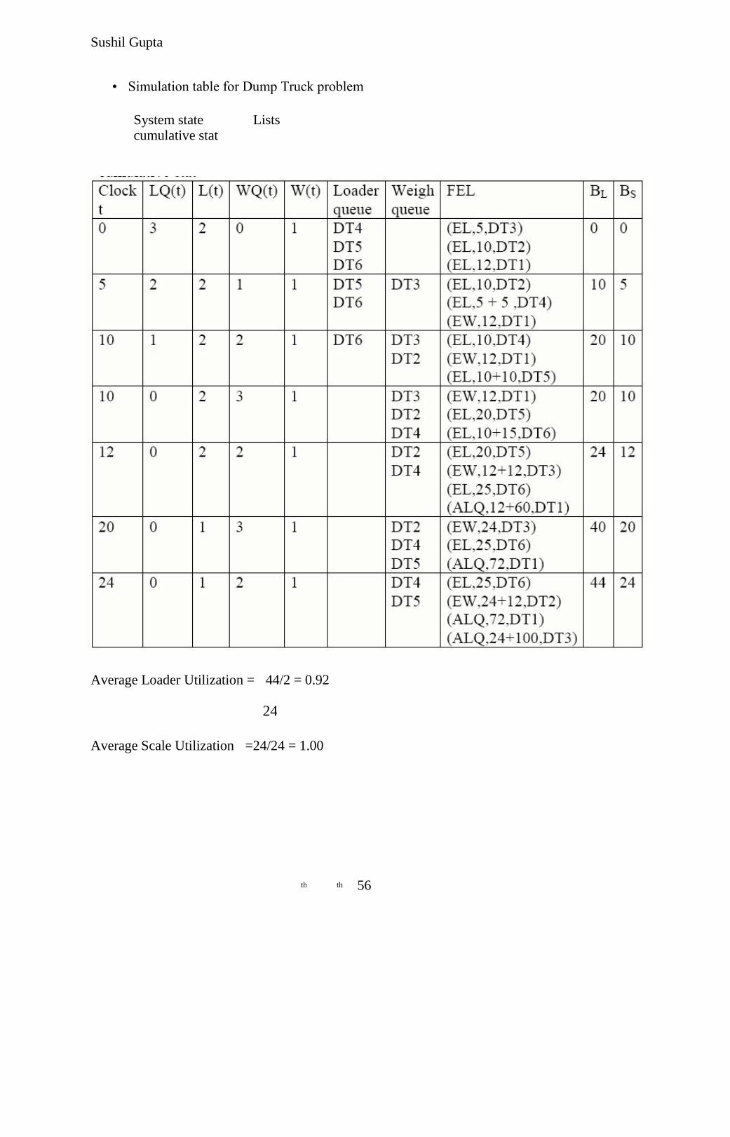
• Simulation table for Dump Truck problem
System state Lists
cumulative stat
Average Loader Utilization = 44/2 = 0.92
24
Average Scale Utilization =24/24 = 1.00
56 th th
Sushil Gupta
CHAPTER – 4
RANDOM-NUMBER GENERATION
Ran dom numbers are a necessary basic ingredient in the simulation of
almost all discrete systems. Most computer languages have a subroutine, object, or
function that will generate a random number. Similarly simulation languages
generate random numbers that arc used to generate event limes and other random
variables.
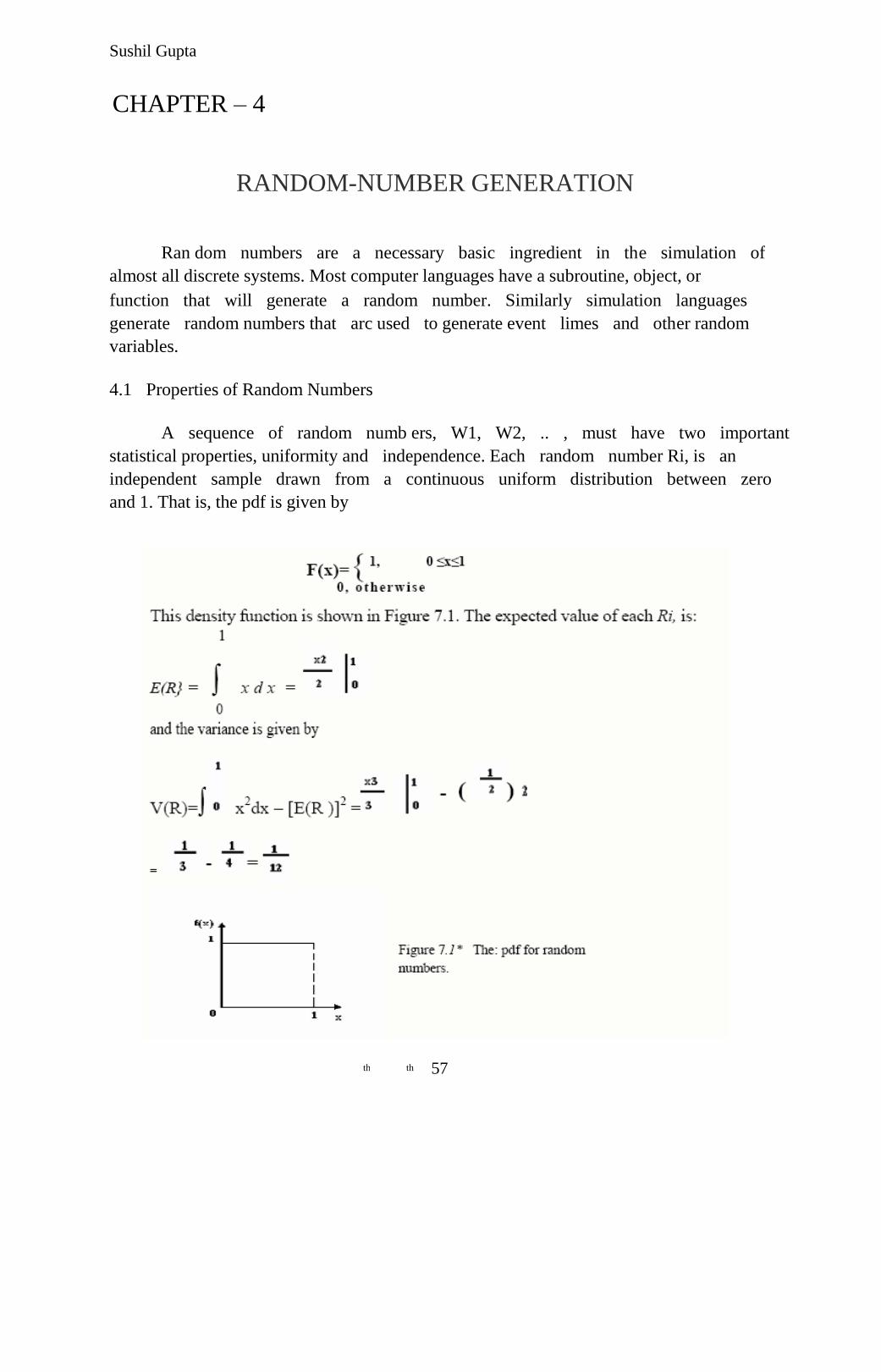
4.1 Properties of Random Numbers
A sequence of random numb ers, W1, W2, .. , must have two important
statistical properties, uniformity and independence. Each random number Ri, is an
independent sample drawn from a continuous uniform distribution between zero
and 1. That is, the pdf is given by
57 th th
Sushil Gupta
Some consequences of the uniformity and independence properties are the
following:
1. If the interval (0,1) is divided into n classes, or subintervals of equal length, the
expected number of observations m each interval ii N/n where A' is the total number
of observations.
2. The probability of observing a value in a particular interval is of the previous values
drawn
4.2 Generation of Pseudo-Random Numbers
Pseudo means false,so false random numbers are being generated.The goal of any
generation scheme, is to produce a sequence of numbers belween zero and 1 which
simulates, or initates, the ideal properties of uniform distribution and independence as
closely as possible.
When generating pseudo-random numbers, certain problems or errors can occur.
These errors, or departures from ideal randomness, are all related to the properties stated
previously. Some examples include the following
1. The generated numbers may not be uniformly distributed.
2. The generated numbers may be discrete -valued instead continuous valued
3. The mean of the generated numbers may be too high or too low. 4. The variance of the generated numbers may be too high or low
5. There may be dependence. The following are examples:
(a) Autocorrelation between numbers.
(b) Numbers successively higher or lower than adjacent numbers. (c) Several numbers above the mean followed by several numbers below the
mean.
Usually, random numbers are generated by a digital computer as part of the
simulation.
Numerous methods can be used to generate the values. In selecting among these methods,
or routines, there are a number of important considerations.
1. The routine should be fast. . The total cost can be managed by selecting a
computationally efficient method of random-number generation. 2. The routine should be portable to different computers, and ideally to different
programming languages .This is desirable so that the simulation program produces the
same results wherever it is executed.
3. The routine should have a sufficiently long cycle. The cycle length, or period, represents
the length of the random-number sequence before previous numbers begin to repeat
58 th th
Sushil Gupta
themselves in an earlier order. Thus, if 10,000 events are to be generated, the period
should be many times that long,
A special case cycling is degenerating. A routine degenerates when the same
random numbers appear repeatedly. Such an occurrence is certainly unacceptable. This
can happen rapidly with some methods.
4. The random numbers should be replicable. Given the starting point (or conditions), it
should be possible to generate the same set of random numbers, completely independent
of the system that is being simulated. This is helpful for debugging purpose and is a
means of facilitating comparisons between systems.
5. Most important, and as indicated previously, the generated random numbers should
closely approximate the ideal statistical properties of uniformity and independences
4.3 Techniques for Generating Random Numbers
The linear congruential method, initially proposed by Lehmer [1951], produces a sequence of
integers, X\, X2,... between zero and m — 1 according to the following recursive relationship:
X = (a Xi + c) mod m, i = 0,1, 2,...(7.1) i+1
The initial value X is called the seed, a is called the constant multiplier, c is the increment, and 0 m is the modulus.
If c 0 in Equation (7.1), the form is called the mixed congruential method. When c = 0, the
form is known as the multiplicative congruential method. The selection of the values for a, c, m
and Xo drastically affects the statistical properties and the cycle length. . An example will illustrate how this technique operates.
EXAMPLE 4.1
Use the linear congruential method to generate a sequence of random numbers with = 27, X 0
a= 17, c = 43, and m = 100. Here, the integer values generated will all be between zer o and 99
because of the value of the modulus . These random integers should appear to be uniformly
distributed the integers zero to 99.Random numbers between zero and 1 can be generated by
R =X /m, i= 1,2,…… (7.2) i i
The sequence of X and subsequent R values is computed as follows: i i
X = 27 0
X = (17.27 + 43) mod 100 = 502 mod 100 = 2 1 R 2/100=0. 02 1=
X = (17 • 2 + 43) mod 100 = 77 mod 100 = 77 2
R 77 /100=0. 77 2=
*[3pt] X = (17•77+ 43) mod 100 = 1352 mod 100 = 52 3 R =52 /100=0. 52 3
59 th th
Sushil Gupta
First, notice that the numbers generated from Equation (7.2) can only assume values from
the set I = {0,1 /m, 2/m,..., (m — l)/m), since each Xi is an integer in the set {0,1,2,..., m — 1}.
Thus, each Ri is discrete on I, instead of continuous on the interval [0, 1], This approximation
appears to be of little consequence, provided that the modulus m is a very large integer. (Values
such as m = 2 — 1 and m = 2 are in common use in generators appearing in many simulation 31 48
languages.) By maximum density is meant that the values assumed by Ri = 1, 2,..., leave no large
gaps on [0,1]
Second, to help achieve maximum density, and to avoid cycling (i.e., recurrence of the
same sequence of generated numbers) in practical applications, the generator should have the
largest possible period. Maximal period can be achieved by the proper choice of a, c, m, and . X 0
• For m a power of 2, say m =2 and c 0, the longest possible period is P = m = 2 , which b b is achieved provided that c is relatively prime to m (that is, the greatest common factor of
c and m i s l ), and =a = l+4k, where k is an integer.
• For m a power of 2, say m =2 and c = 0, the longest possible period is P = m/4 = 2 , b b-2
X which is achieved provided that the seed is odd and the multiplier ,a, is given by 0
a=3+8K , for some
K=0,1,..
• For m a prime number and c=0, the longest possible period is P=m-1, which is achieved
provided that the multiplier , a, has the property that the smallest integer k such that
a - 1is divisible by m is k= m-1. k
EXAMPLE 4.3
Let m = 102 = 100, a = 19, c = 0, and X0 = 63, and generate a sequence c random integers using
Equation (7.1).
X = 63 0 X = (19)(63) mod 100 = 1197 mod 100 = 97 1
X = (19) (97) mod 100 = 1843 mod 100 = 43 2
X = (19) (43) mod 100 = 817 mod 100 = 17 3
.
. .
.
When m is a power of 10, say m = 10 , the modulo operation is accomplished by saving b the b rightmost (decimal) digits.
EXAMPLE 4.4
60 th th
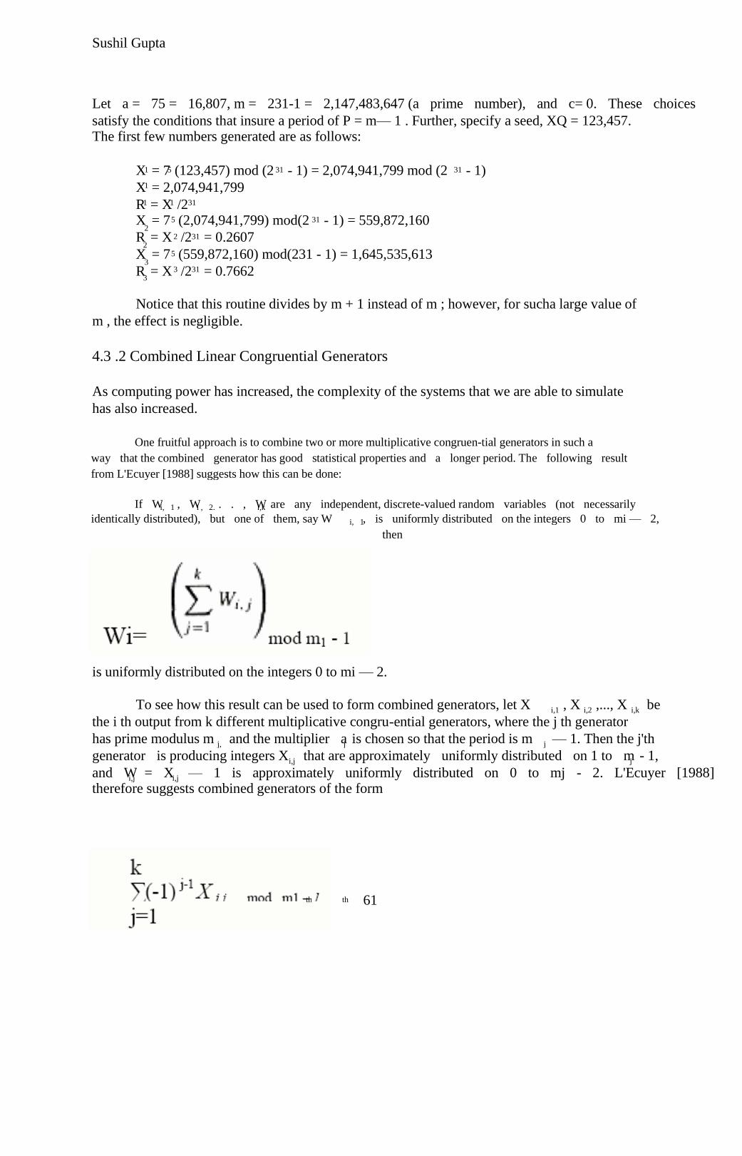
Sushil Gupta
Let a = 75 = 16,807, m = 231-1 = 2,147,483,647 (a prime number), and c= 0. These choices
satisfy the conditions that insure a period of P = m— 1 . Further, specify a seed, XQ = 123,457. The first few numbers generated are as follows:
X = 7 (123,457) mod (2 - 1) = 2,074,941,799 mod (2 - 1) 1 5 31 31
X = 2,074,941,799 1
R = X /2 1 1 31
X = 7 (2,074,941,799) mod(2 - 1) = 559,872,160 5 31 2
R = X /2 = 0.2607 2 31 2
X = 7 (559,872,160) mod(231 - 1) = 1,645,535,613 5 3
R = X /2 = 0.7662 3 31 3
Notice that this routine divides by m + 1 instead of m ; however, for sucha large value of
m , the effect is negligible.
4.3 .2 Combined Linear Congruential Generators
As computing power has increased, the complexity of the systems that we are able to simulate
has also increased.
One fruitful approach is to combine two or more multiplicative congruen-tial generators in such a
way that the combined generator has good statistical properties and a longer period. The following result
from L'Ecuyer [1988] suggests how this can be done:
If W , W . . , W are any independent, discrete-valued random variables (not necessarily i, 1 i , 2. i,k identically distributed), but one of them, say W , is uniformly distributed on the integers 0 to mi — 2, i, 1
then
is uniformly distributed on the integers 0 to mi — 2.
To see how this result can be used to form combined generators, let X , X ,..., X be i,1 i,2 i,k
the i th output from k different multiplicative congru-ential generators, where the j th generator
has prime modulus m and the multiplier a is chosen so that the period is m — 1. Then the j'th j, j j
generator is producing integers X that are approximately uniformly distributed on 1 to m - 1, i,j j
and W = X — 1 is approximately uniformly distributed on 0 to mj - 2. L'Ecuyer [1988] i,j i,j therefore suggests combined generators of the form
61 th th
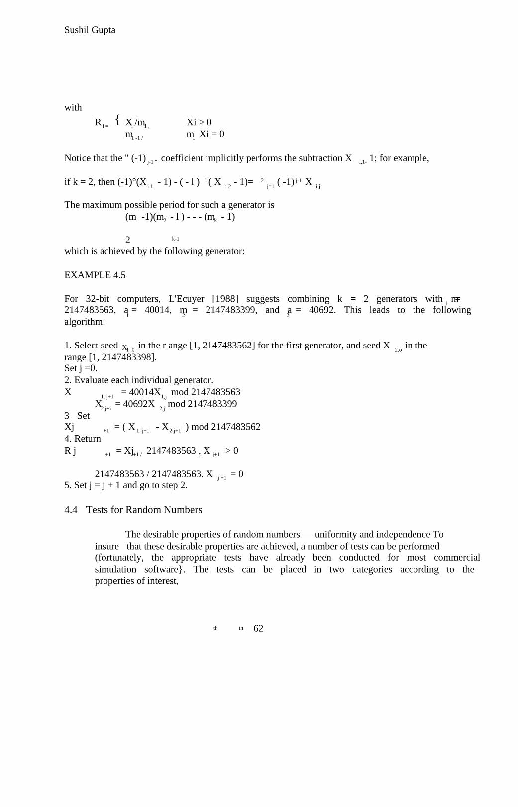
Sushil Gupta
with
{ R X /m Xi > 0 i = i 1 ,
m m Xi = 0 1 -1 / 1
Notice that the " (-1) coefficient implicitly performs the subtraction X 1; for example, j-1 " i,1-
if k = 2, then (-1)°(X - 1) - ( - l ) ( X - 1)= ( -1) X l 2 j-1 i 1 i 2 j=1 i,j
The maximum possible period for such a generator is
(m -1)(m - l ) - - - (m - 1) 1 2 k
2 k-1
which is achieved by the following generator:
EXAMPLE 4.5
For 32-bit computers, L'Ecuyer [1988] suggests combining k = 2 generators with m = 1
2147483563, a = 40014, m = 2147483399, and a = 40692. This leads to the following 1 2 2
algorithm:
1. Select seed in the r ange [1, 2147483562] for the first generator, and seed X in the X 1 ,0 2.o range [1, 2147483398]. Set j =0.
2. Evaluate each individual generator.
X = 40014X mod 2147483563 1, j+1 1,j
X = 40692X mod 2147483399 2,j+i 2,j
3 Set Xj = ( X - X ) mod 2147483562 +1 1, j+1 2 j+1
4. Return
R j = Xj 2147483563 , X > 0 +1 +1 / j+1
2147483563 / 2147483563. X = 0 j +1 5. Set j = j + 1 and go to step 2.
4.4 Tests for Random Numbers
The desirable properties of random numbers — uniformity and independence To
insure that these desirable properties are achieved, a number of tests can be performed
(fortunately, the appropriate tests have already been conducted for most commercial
simulation software}. The tests can be placed in two categories according to the
properties of interest,
62 th th
Sushil Gupta
The first entry in the list below concerns testing for uniformity. The second
through fifth entries concern testing for independence. The five types of tests
1. Frequency test Uses the Kolmogorov-Smirnov or the chi- square test to compare
the distribution of the set of numbers generated to a uniform distribution.
2. Runs test. Tests the runs up and down or the runs above, and below the mean by
comparing the actual values to expected values. The statistic for comparison is the
chi-square. 3. Autocorrelation test Tests the correlation between numbers and compares the
sample correlation to the expected correlation of zero.
4. Gap test. Counts the number of digits that appear between repetitions of
particular digit and then uses the Kolmogorov-Smirnov test to compare with the
expected size of gaps, 5. Poker test . Treats numbers grouped together as a poker hand. Then the hands
obtained are compared to what is expected using the chi-square test.
In testing for uniformity, the hypotheses are as follows:
H : R ~ U/[0,1] 0 i
H : R ~U/[0,l] 1 i
The null hypothesis, H reads that the numbers are distributed uniformly on the 0
interval [0,1]. Failure to reject the null hypothesis means that no evidence of
nonuniformity has been detected on the basis of this test. This does not imply that further
testing of the generator for uniformity is unnecessary.
In testing for independence, the hypotheses are as follows:
: Ri ~ independently H 0 H :Ri~independently 1
This null hypothesis reads that the numbers are independent. Failure to reject the null H 0
hypothesis means that no evidence of dependence has been detected on the basis of this test. This
does not imply that further testing of the generator for independence is unnecessary.
For each test, a level of significance a must be stated. The level a is the probability of
rejecting the null hypothesis given that the null hypothesis is true, or
a = P (reject | true) H H 0 0
The decision maker sets the value of & for any test. Frequently, a is set to 0.01 orO.05. If
several tests are conducted on the same set of numbers, the probability of r ejecting the null
hypothesis on at least one test, by chance alone [i.e., making a Type I (a) error], increases. Say
that a= 0.05 and that five different tests are conducted on a sequence of numbers. The probability
of rejecting the null hypothesis on at least one test, by chance alone, may be as large as 0.25.
4.4 .1 Frequency Tests
63 th th
Sushil Gupta
A basic test that should always be performed to validate a new generator is the test of
uniformity. Two different methods of testing are available. They are the Kolmogorov-Smirnov
and the chi-square test. Both of these tests measure the degree of agreement between the
distribution of a sample of generated random numbers and the theoretical uniform distribution.
Both tests are ased on the null hypothesis of no significant difference between the sample
distribution and the theoretical distribution.
1. The Kolmogorov-Smirnov test. This test compares the continuous cdf, ( ), of the F X
uniform distribution to the empirical cdf, S (x), of the sample of N observations. By definition, N
F(x) = x, 0 <= x <= 1
If the sample from the random-number generator is ,• • •, , then the empirical cdf, R R RN 1 2,
( ), is defined by S X N
( ) = number of ,• • •, Rn which are <= x S X R R 1 2, N
N
As N becomes larger, ( ) should become a better approximation to F(X) , provided that S X N the null hypothesis is true.
The Kolmogorov-Smirnov test is based on the largest absolute deviation between F(x)
and ( ) over the range of the r andom variable. That is.it is based on the statistic S X N
D = max | F(x) - S (x)| (7.3) N
For testing against a uniform cdf, the test procedure follows these steps:
Step 1. Rank the data from smallest to largest. Let R denote the i th smallest (i)
observation, so that
R <= R <= • • • <= R (1) (2 ) (N)
Step 2. Compute
{ D = i/N - R } + max (i)
<= i <= 1 N
Step3. Compute D = max(D , D ). + -
Step 4. Determine the critical value, D , from Table A.8 for the specified significance a
level a and the given sample size N.
64 th th
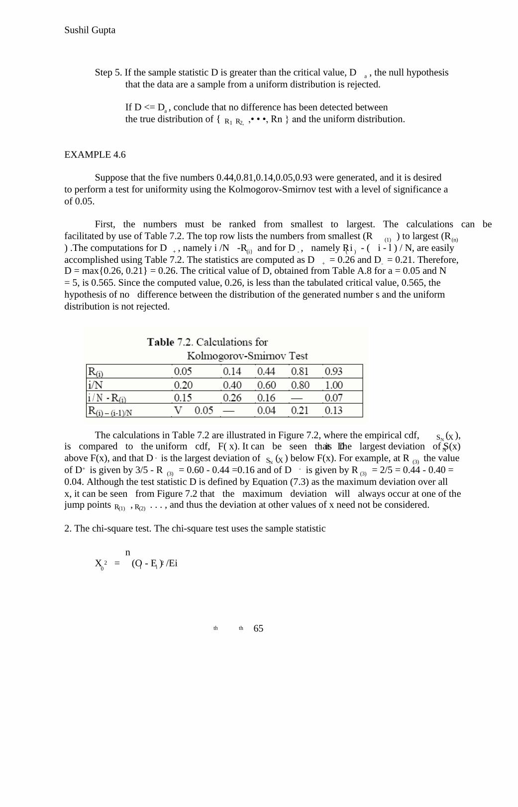
Sushil Gupta
Step 5. If the sample statistic D is greater than the critical value, D , the null hypothesis a
that the data are a sample from a uniform distribution is rejected.
If D <= D , conclude that no difference has been detected between a
the true distribution of { ,• • •, Rn } and the uniform distribution. R R 1 2,
EXAMPLE 4.6
Suppose that the five numbers 0.44,0.81,0.14,0.05,0.93 were generated, and it is desired
to perform a test for uniformity using the Kolmogorov-Smirnov test with a level of significance a
of 0.05.
First, the numbers must be ranked from smallest to largest. The calculations can be
facilitated by use of Table 7.2. The top row lists the numbers from smallest (R ) to largest (R (1) (n)
) .The computations for D , namely i /N -R and for D , namely R i - ( i - l ) / N, are easily + (i} - ( )
accomplished using Table 7.2. The statistics are computed as D = 0.26 and D = 0.21. Therefore, + - D = max{0.26, 0.21} = 0.26. The critical value of D, obtained from Table A.8 for a = 0.05 and N
= 5, is 0.565. Since the computed value, 0.26, is less than the tabulated critical value, 0.565, the
hypothesis of no difference between the distribution of the generated number s and the uniform
distribution is not rejected.
The calculations in Table 7.2 are illustrated in Figure 7.2, where the empirical cdf, ( ), S X N is compared to the uniform cdf, F( x). It can be seen that D is the largest deviation of S (x) +
N
above F(x), and that D is the largest deviation of ( ) below F(x). For example, at R the value - S X (3) N of D is given by 3/5 - R = 0.60 - 0.44 =0.16 and of D is given by R = 2/5 = 0.44 - 0.40 = + -
(3) (3)
0.04. Although the test statistic D is defined by Equation (7.3) as the maximum deviation over all
x, it can be seen from Figure 7.2 that the maximum deviation will always occur at one of the
jump points , . . . , and thus the deviation at other values of x need not be considered. R R (1) (2)
2. The chi-square test. The chi-square test uses the sample statistic
n
X = (O - E ) /Ei 2 2 i i 0
65 th th
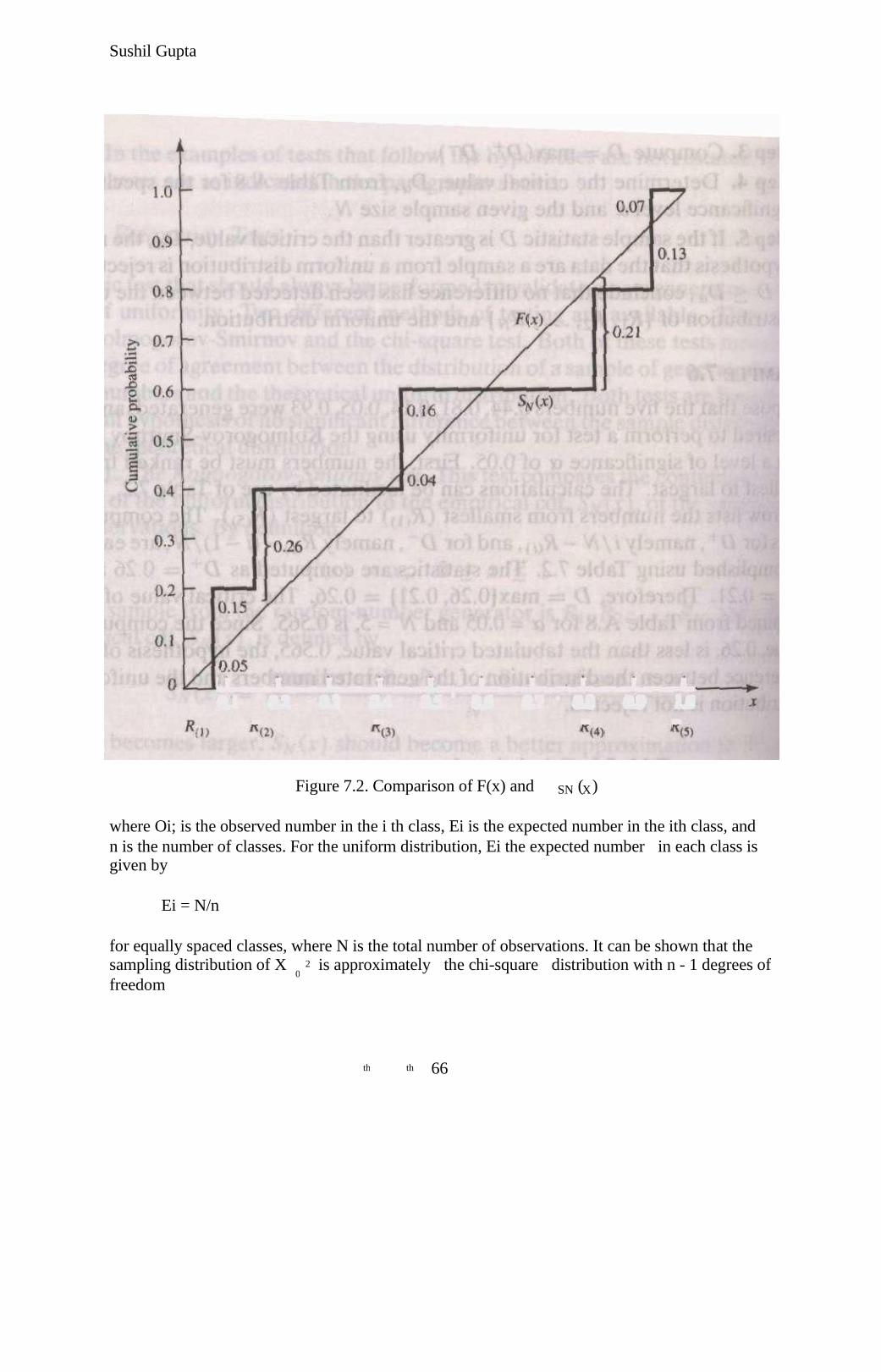
Sushil Gupta
Figure 7.2. Comparison of F(x) and ( ) SN X
where Oi; is the observed number in the i th class, Ei is the expected number in the ith class, and
n is the number of classes. For the uniform distribution, Ei the expected number in each class is
given by
Ei = N/n
for equally spaced classes, where N is the total number of observations. It can be shown that the
sampling distribution of X is approximately the chi-square distribution with n - 1 degrees of 2 0
freedom
66 th th
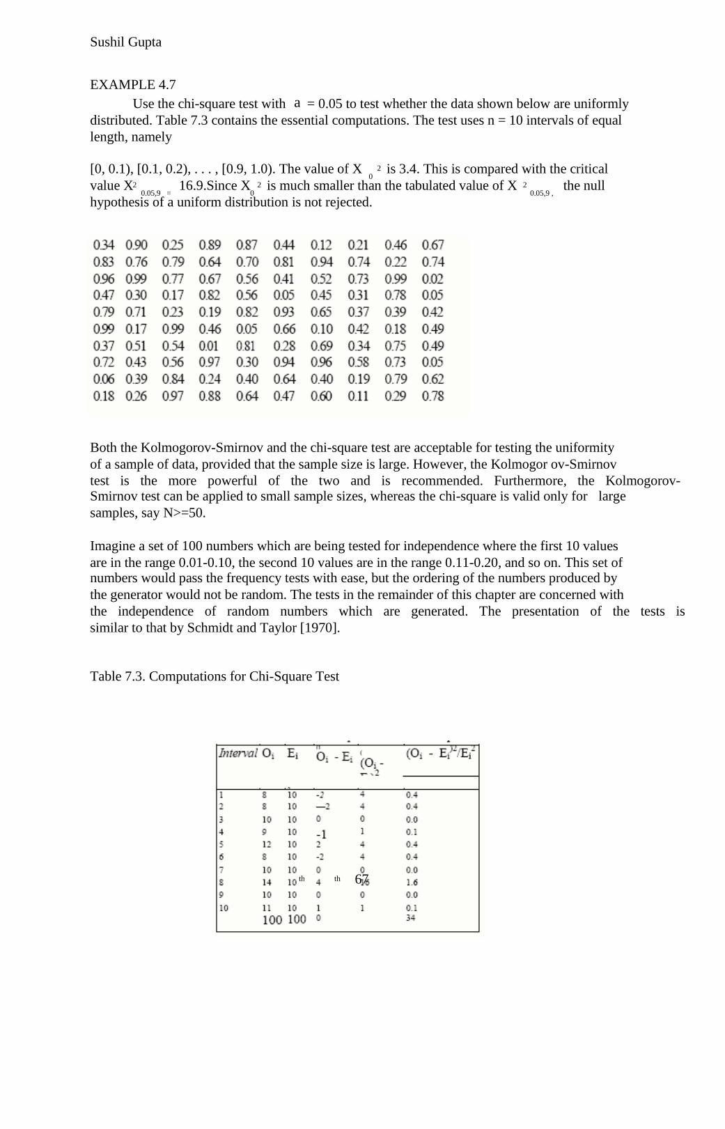
Sushil Gupta
EXAMPLE 4.7
a Use the chi-square test with = 0.05 to test whether the data shown below are uniformly
distributed. Table 7.3 contains the essential computations. The test uses n = 10 intervals of equal
length, namely
[0, 0.1), [0.1, 0.2), . . . , [0.9, 1.0). The value of X is 3.4. This is compared with the critical 2 0
value X 16.9.Since X is much smaller than the tabulated value of X the null 2 2 2 0.05,9 = 0 0.05,9 ,
hypothesis of a uniform distribution is not rejected.
Both the Kolmogorov-Smirnov and the chi-square test are acceptable for testing the uniformity
of a sample of data, provided that the sample size is large. However, the Kolmogor ov-Smirnov
test is the more powerful of the two and is recommended. Furthermore, the Kolmogorov-
Smirnov test can be applied to small sample sizes, whereas the chi-square is valid only for large
samples, say N>=50.
Imagine a set of 100 numbers which are being tested for independence where the first 10 values
are in the range 0.01-0.10, the second 10 values are in the range 0.11-0.20, and so on. This set of
numbers would pass the frequency tests with ease, but the ordering of the numbers produced by
the generator would not be random. The tests in the remainder of this chapter are concerned with
the independence of random numbers which are generated. The presentation of the tests is
similar to that by Schmidt and Taylor [1970].
Table 7.3. Computations for Chi-Square Test
67 th th
Sushil Gupta
4.4 .2 Runs Tests
1. Runs up and runs down. Consider a generator that provided a set of 40 numbers in the
following sequence:
0.08 0.09 0.23 0.29 0.42 0.55 0.58 0.72 0.89 0.91
0.11 0.16 0.18 0.31 0.41 0.53 0.71 0.73 0.74 0.84
0.02 0.09 0.30 0.32 0.45 0.47 0.69 0.74 0.91 0.95
0.12 0.13 0.29 0.36 0.38 0.54 0.68 0.86 0.88 0.91
Both the Kolmogorov-Smirnov test and the chi-square test would indicate that the
numbers are uniformly distributed. However, a glance at the ordering shows that the
numbers are successively larger in blocks of 10 values. If these numbers are rearranged
as follows, there is far less reason to doubt their independence
0.41 0.68 0.89 0.84 0.74 0.91 0.55 0.71 0.36 0.30
0.09 0.72 0.86 0.08 0.54 0.02 0.11 0.29 0.16 0.18
0.88 0.91 0.95 0.69 0.09 0.38 0.23 0.32 0.91 0.53
0.31 0.42 0.73 0.12 0.74 0.45 0.13 0.47 0.58 0.29
The runs test examines the arrangement of numbers in a sequence to test the hypothesis of
independence.
Before defining a run, a look at a sequence of coin tosses will help with some terminology.
Consider the following sequence generated by tossing a coin 10 times:
H T T H H T T T H T
There are three mutually exclusive outcomes, or events, with respect to the sequence. Two of the
possibilities are rather obvious. That is, the toss can result in a head or a tail. The third possibility
is "no event." The first head is preceded by no event and the last tail is succeeded by no event.
Every sequence begins and ends with no event.
A run is defined as a succession of similar events preceded and followed by a different event.
The length of the run is the number of events that occur in the run. In the coin-flipping example
above there are six runs. The first run is of length one, the second and third of length two, the
fourth of length three. and the fifth and sixth of length one.
68 th th
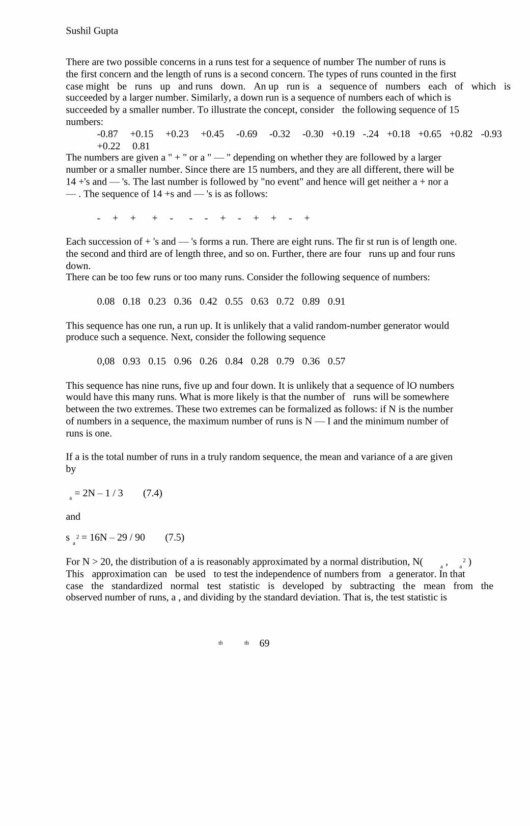
Sushil Gupta
There are two possible concerns in a runs test for a sequence of number The number of runs is
the first concern and the length of runs is a second concern. The types of runs counted in the first
case might be runs up and runs down. An up run is a sequence of numbers each of which is
succeeded by a larger number. Similarly, a down run is a sequence of numbers each of which is
succeeded by a smaller number. To illustrate the concept, consider the following sequence of 15
numbers:
-0.87 +0.15 +0.23 +0.45 -0.69 -0.32 -0.30 +0.19 -.24 +0.18 +0.65 +0.82 -0.93
+0.22 0.81
The numbers are given a " + " or a " — " depending on whether they are followed by a larger
number or a smaller number. Since there are 15 numbers, and they are all different, there will be
14 +'s and — 's. The last number is followed by "no event" and hence will get neither a + nor a
— . The sequence of 14 +s and — 's is as follows:
- + + + - - - + - + + - +
Each succession of + 's and — 's forms a run. There are eight runs. The fir st run is of length one.
the second and third are of length three, and so on. Further, there are four runs up and four runs
down. There can be too few runs or too many runs. Consider the following sequence of numbers:
0.08 0.18 0.23 0.36 0.42 0.55 0.63 0.72 0.89 0.91
This sequence has one run, a run up. It is unlikely that a valid random-number generator would
produce such a sequence. Next, consider the following sequence
0,08 0.93 0.15 0.96 0.26 0.84 0.28 0.79 0.36 0.57
This sequence has nine runs, five up and four down. It is unlikely that a sequence of lO numbers
would have this many runs. What is more likely is that the number of runs will be somewhere
between the two extremes. These two extremes can be formalized as follows: if N is the number
of numbers in a sequence, the maximum number of runs is N — I and the minimum number of
runs is one.
If a is the total number of runs in a truly random sequence, the mean and variance of a are given
by
= 2N – 1 / 3 (7.4) a
and
s = 16N – 29 / 90 (7.5) 2 a
For N > 20, the distribution of a is reasonably approximated by a normal distribution, N( , ) 2 a a
This approximation can be used to test the independence of numbers from a generator. In that
case the standardized normal test statistic is developed by subtracting the mean from the
observed number of runs, a , and dividing by the standard deviation. That is, the test statistic is
69 th th
Sushil Gupta
Z = a - / 0 a a
Substituting Equation (7,4) for and the square root of Equation (7.5) for yields a a
Z = a - [( 2N - 1)/3] / sqrt((16N – 29) / 90 ) 0
where Zo ~ N(0 1). Failure to reject the hypothesis of independence occur when — z / 2 <= Zo a
<= z / 2 where a is the level of significance. The critical values and rejection region are shown in a Figure 7.3.
Failure to reject Figure 7.3.
2. Runs above and below the mean. The test for runs up and runs down is not completely
adequate to assess the independence of a group of numbers.
Consider the following 40 numbers:
0.63 0.72 0.79 0.81 0.52 0.94 0.8.1 0.93 0.87 0.67
0.54 0.83 0.89 0.55 0.88 0.77 0.74 0.95 0.82 0.86
0.43 0.32 0.36 0.18 0.08 0.19 0.18 0.27 0.36 0.34
0.31 0.45 0.49 0.43 0.46 0.35 0.25 0.39 0.47 0.41
The sequence of runs up and runs down is as follows:
+ + + - + - + - - - + + - + - - + - + - - + - - + - + + - - + + - + - - + + -
This sequence is exactly the same as that in Example 7.8. Thus, the numbers would pass the
runs-up and runs-down test. However, it can be observed that the first 20 numbers are all above
the mean [(0.99 + O.OO)/2 = 0.495] and the last 20 numbers are all below the mean. Such an
occurrence is highly unlikely. The previous runs analysis can be used to test for this condition, if
the definition of a run is changed. Runs will be described as being above the mean or below the
mean. A " + " sign will be used to denote an observation above the mean, and a "-" sign will
denote an observation below the mean.
For example, consider the following sequence of 20 two-digit random numbers;
0.40 0.84 0.75 0.18 0.13 0.92 0.57 0.77 0.30 0.71
70 th th
Sushil Gupta
0.42 0.05 0.78 0.74 0.68 0.03 0.18 0.51 0.10 0.37
The pluses and minuses are as follows:
- + + - - + + + - + - - + + + - - + - -
In this case, there is a run of length one below the mean followed by a run of length two above
the mean, and so on. In all. there are 11 runs, five of which are above the mean and six of which
are below the mean. Let n1 and n2 be the number of individual observations above and below the
mean and let b be the total number of runs. Notice that the maximum number of runs is N = n1 +
n2 and the minimum number of runs is one.
Given n1 and n2. the mean — with a continuity correction suggested by Swed and Eisenhart [1943] —and the variance of b for a truly independent sequence are given by
=2 n n / N +1/2 (7.6) b 1 2
and
= 2 (2 -N) / N (N – 1) (7.7) 2 b n1n2 n1n2 2
For either n1 or n2 greater than 20, b is approximately normally distributed. The test statistic can
be formed by subtracting the mean from the number of runs and dividing by the standard
deviation, or
Z = (b-(2 /N)-1/2) / [2 (2n1n2-N/N (N-1)] 2 ½ 0 n1n2 n1n2
Failure to reject the hypothesis of independence occurs when —z /2 <= Z < =z /2-, where a is a 0 a
the level of significance.
EXAMPLE 4.9
Determine whether there is an excessive number of runs above or below the mean for the
sequence of numbers given in Example 7.8. The assignment of + 's and — 's results in the
following:
- + + + + + + + - - - + + - + - - - - - - - + +
- - - - + + - - + - + - - + + -
The values of n1 ,n2 , and b are as follows:
n = 18 1
n = 22 2
N = n +n = 40 1 2
b = 17
Equations (7.6) and (7.7) are used to determine and as follows: 2 b b
= 2(18)(22)/40 + 1/2 = 20.3 b
= 2(18)(22)[(2)(18)(22)-40] /(40) (40-1)=9.54 2 2 b
71 th th
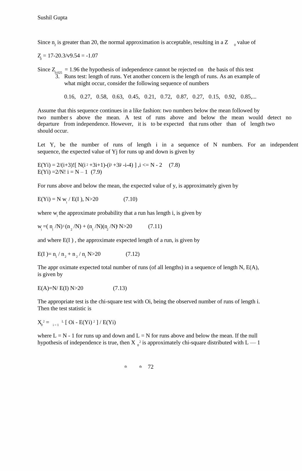
Sushil Gupta
Since n is greater than 20, the normal approximation is acceptable, resulting in a Z value of 2 0
Z = 17-20.3/v9.54 = -1.07 0
Since Z = 1.96 the hypothesis of independence cannot be rejected on the basis of this test 0.025 3. Runs test: length of runs. Yet another concern is the length of runs. As an example of
what might occur, consider the following sequence of numbers
0.16, 0.27, 0.58, 0.63, 0.45, 0.21, 0.72, 0.87, 0.27, 0.15, 0.92, 0.85,...
Assume that this sequence continues in a like fashion: two numbers below the mean followed by
two number s above the mean. A test of runs above and below the mean would detect no
departure from independence. However, it is to be expected that runs other than of length two
should occur.
Let Y, be the number of runs of length i in a sequence of N numbers. For an independent
sequence, the expected value of Yj for runs up and down is given by
E(Yi) = 2/(i+3)![ N(i +3i+1)-(i +3i -i-4) ] ,i <= N - 2 (7.8) 2 3 2
E(Yi) =2/N! i = N – 1 (7.9)
For runs above and below the mean, the expected value of y, is approximately given by
E(Yi) = N w / E(I ), N>20 (7.10) i
where w the approximate probability that a run has length i, is given by i
w =( n /N) (n /N) + (n /N)(n /N) N>20 (7.11) I I i 1 2 1 2
and where E(I ) , the approximate expected length of a run, is given by
E(I )= n / n + n / n N>20 (7.12) 1 2 2 1
The appr oximate expected total number of runs (of all lengths) in a sequence of length N, E(A),
is given by
E(A)=N/ E(I) N>20 (7.13)
The appropriate test is the chi-square test with Oi, being the observed number of runs of length i.
Then the test statistic is
X = [ Oi - E(Yi) ] / E(Yi) 2 L 2 0 i = 1
where L = N - 1 for runs up and down and L = N for runs above and below the mean. If the null
hypothesis of independence is true, then X is approximately chi-square distributed with L — 1 2 0
72 th th
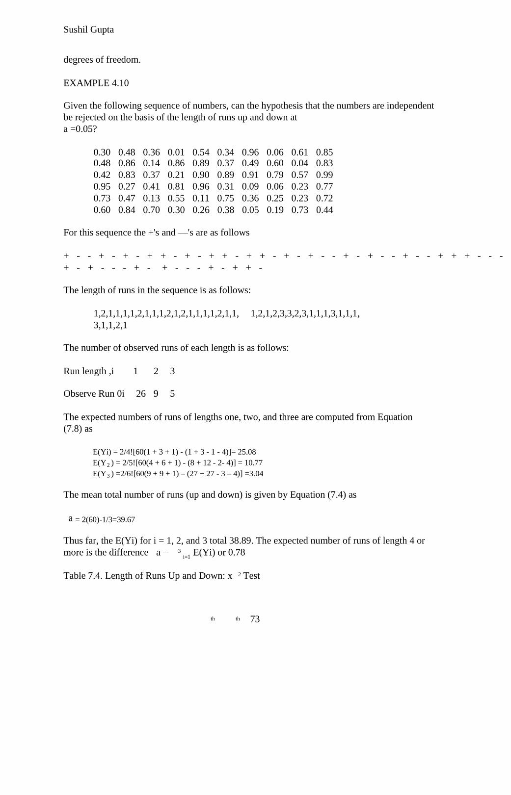
Sushil Gupta
degrees of freedom.
EXAMPLE 4.10
Given the following sequence of numbers, can the hypothesis that the numbers are independent
be rejected on the basis of the length of runs up and down at
a =0.05?
0.30 0.48 0.36 0.01 0.54 0.34 0.96 0.06 0.61 0.85
0.48 0.86 0.14 0.86 0.89 0.37 0.49 0.60 0.04 0.83
0.42 0.83 0.37 0.21 0.90 0.89 0.91 0.79 0.57 0.99
0.95 0.27 0.41 0.81 0.96 0.31 0.09 0.06 0.23 0.77
0.73 0.47 0.13 0.55 0.11 0.75 0.36 0.25 0.23 0.72
0.60 0.84 0.70 0.30 0.26 0.38 0.05 0.19 0.73 0.44
For this sequence the +'s and —'s are as follows
+ - - + - + - + + - + - + + - + + - + - + - - + - + - - + - - + + + - - - + + - - -
+ - + - - - + - + - - - + - + + -
The length of runs in the sequence is as follows:
1,2,1,1,1,1,2,1,1,1,2,1,2,1,1,1,1,2,1,1, 1,2,1,2,3,3,2,3,1,1,1,3,1,1,1,
3,1,1,2,1
The number of observed runs of each length is as follows:
Run length ,i 1 2 3
Observe Run 0i 26 9 5
The expected numbers of runs of lengths one, two, and three are computed from Equation
(7.8) as
E(Yi) = 2/4![60(1 + 3 + 1) - (1 + 3 - 1 - 4)]= 25.08
E(Y ) = 2/5![60(4 + 6 + 1) - (8 + 12 - 2- 4)] = 10.77 2
E(Y ) =2/6![60(9 + 9 + 1) – (27 + 27 - 3 – 4)] =3.04 3
The mean total number of runs (up and down) is given by Equation (7.4) as
a = 2(60)-1/3=39.67
Thus far, the E(Yi) for i = 1, 2, and 3 total 38.89. The expected number of runs of length 4 or
more is the difference a – E(Yi) or 0.78 3 i=1
Table 7.4. Length of Runs Up and Down: x Test 2
73 th th
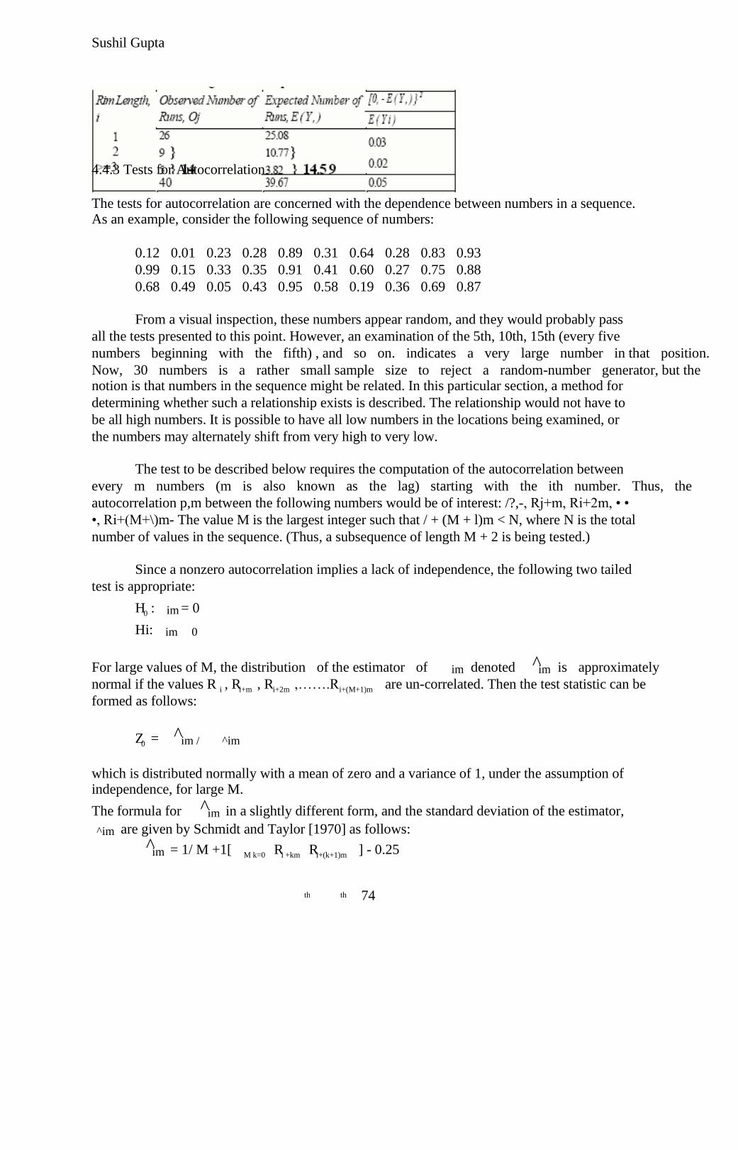
Sushil Gupta
4.4.3 Tests for Autocorrelation
The tests for autocorrelation are concerned with the dependence between numbers in a sequence. As an example, consider the following sequence of numbers:
0.12 0.01 0.23 0.28 0.89 0.31 0.64 0.28 0.83 0.93
0.99 0.15 0.33 0.35 0.91 0.41 0.60 0.27 0.75 0.88
0.68 0.49 0.05 0.43 0.95 0.58 0.19 0.36 0.69 0.87
From a visual inspection, these numbers appear random, and they would probably pass
all the tests presented to this point. However, an examination of the 5th, 10th, 15th (every five
numbers beginning with the fifth) , and so on. indicates a very large number in that position.
Now, 30 numbers is a rather small sample size to reject a random-number generator, but the
notion is that numbers in the sequence might be related. In this particular section, a method for
determining whether such a relationship exists is described. The relationship would not have to
be all high numbers. It is possible to have all low numbers in the locations being examined, or
the numbers may alternately shift from very high to very low.
The test to be described below requires the computation of the autocorrelation between
every m numbers (m is also known as the lag) starting with the ith number. Thus, the
autocorrelation p,m between the following numbers would be of interest: /?,-, Rj+m, Ri+2m, • •
•, Ri+(M+\)m- The value M is the largest integer such that / + (M + l)m < N, where N is the total
number of values in the sequence. (Thus, a subsequence of length M + 2 is being tested.)
Since a nonzero autocorrelation implies a lack of independence, the following two tailed
test is appropriate:
H : = 0 im 0
Hi: im 0
^ For large values of M, the distribution of the estimator of denoted is approximately im im
normal if the values R , R , R ,…….R are un-correlated. Then the test statistic can be i i+m i+2m i+(M+1)m
formed as follows:
^ Z = im / ^im 0
which is distributed normally with a mean of zero and a variance of 1, under the assumption of
independence, for large M.
^ The formula for in a slightly different form, and the standard deviation of the estimator, im
are given by Schmidt and Taylor [1970] as follows: ^im
^ = 1/ M +1[ R R ] - 0.25 im M k=0 i +km i+(k+1)m
74 th th
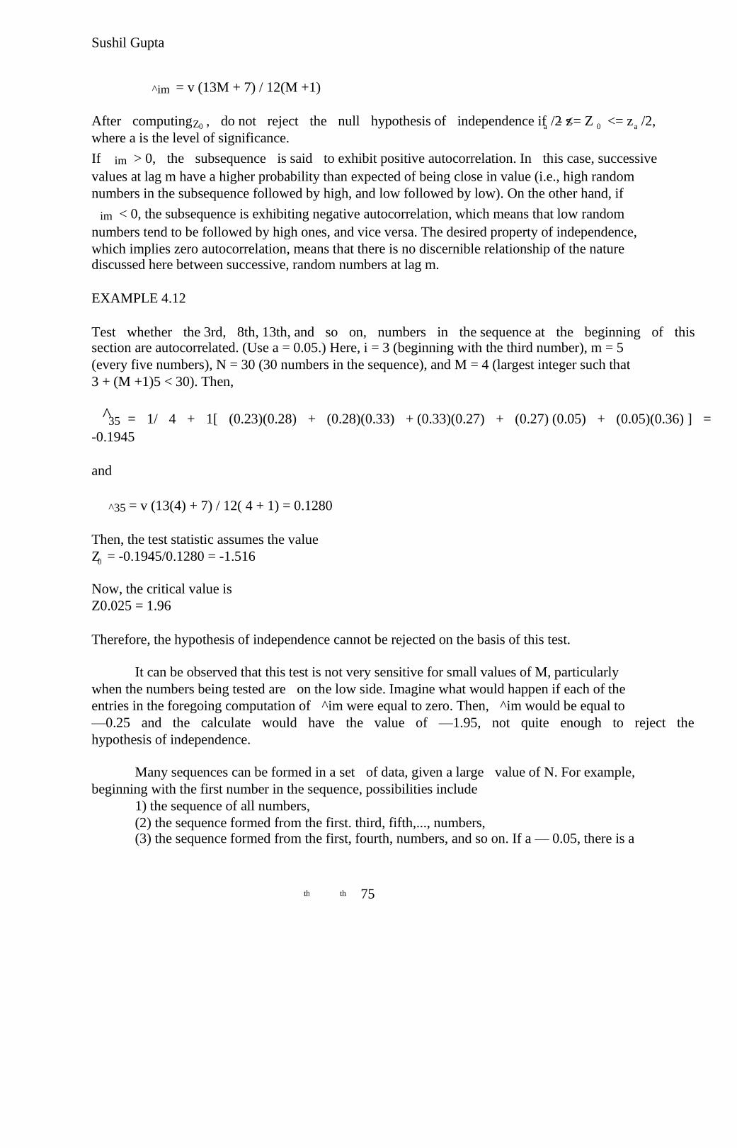
Sushil Gupta
= v (13M + 7) / 12(M +1) ^im
After computing , do not reject the null hypothesis of independence if - z /2 <= Z <= z /2, Z 0 a 0 a
where a is the level of significance.
If > 0, the subsequence is said to exhibit positive autocorrelation. In this case, successive im
values at lag m have a higher probability than expected of being close in value (i.e., high random
numbers in the subsequence followed by high, and low followed by low). On the other hand, if
< 0, the subsequence is exhibiting negative autocorrelation, which means that low random im
numbers tend to be followed by high ones, and vice versa. The desired property of independence,
which implies zero autocorrelation, means that there is no discernible relationship of the nature
discussed here between successive, random numbers at lag m.
EXAMPLE 4.12
Test whether the 3rd, 8th, 13th, and so on, numbers in the sequence at the beginning of this
section are autocorrelated. (Use a = 0.05.) Here, i = 3 (beginning with the third number), m = 5
(every five numbers), N = 30 (30 numbers in the sequence), and M = 4 (largest integer such that
3 + (M +1)5 < 30). Then,
^ = 1/ 4 + 1[ (0.23)(0.28) + (0.28)(0.33) + (0.33)(0.27) + (0.27) (0.05) + (0.05)(0.36) ] = 35
-0.1945
and
= v (13(4) + 7) / 12( 4 + 1) = 0.1280 ^35
Then, the test statistic assumes the value
Z = -0.1945/0.1280 = -1.516 0
Now, the critical value is
Z0.025 = 1.96
Therefore, the hypothesis of independence cannot be rejected on the basis of this test.
It can be observed that this test is not very sensitive for small values of M, particularly
when the numbers being tested are on the low side. Imagine what would happen if each of the
entries in the foregoing computation of ^im were equal to zero. Then, ^im would be equal to
—0.25 and the calculate would have the value of —1.95, not quite enough to reject the
hypothesis of independence.
Many sequences can be formed in a set of data, given a large value of N. For example,
beginning with the first number in the sequence, possibilities include
1) the sequence of all numbers,
(2) the sequence formed from the first. third, fifth,..., numbers, (3) the sequence formed from the first, fourth, numbers, and so on. If a — 0.05, there is a
75 th th
Sushil Gupta
probability of 0.05 of rejecting a true hypothesis. If 10 independent sequences are examined, the
probability of finding no significant autocorrelation, by chance alone, is (0.95) or 0.60. Thus, 10
40% of the time significant autocorrelation would be detected when it does not exist. If a is 0.10
and 10 tests are conducted, there is a 65% chance of finding autocorrelation by chance alone. In
conclusion, when "fishing" for autocorrelation, upon performing numerous tests, autocorrelation
may eventually be detected, perhaps by chance alone, even when no autocorrelation is present.
4.4 .4 Gap Test
The gap test is used to deter.nine the significance of the interval between the recurrences of the
same digit. A gap of length x occurs between the recurrences of some specified digit.
The following example illustrates the length of gaps associated with the digit 3:
4, 1, 3, 5, 1, 7. 2. 8. 2. 0, 7. 9. 1. 3. 5, 2, 7, 9. 4. 1. 6. 3
3, 9. 6, 3, 4. 8, 2. 3, 1, 9, 4. 4, 6. 8. 4, 1, 3. 8. 9. 5. 5. 7
3, 9, 5, 9. 8, 5. 3. 2, 2, 3, 7. 4, 7. 0. 3. 6. 3, 5, 9. 9. 5. 5
5, 0, 4. 6. 8. 0, 4. 7. 0, 3. 3, 0, 9, 5. 7, 9. 5. 1. 6. 6. 3. 8
8, 8, 9, 2, 9. 1. 8. 5, 4. 4. 5, 0, 2. 3, 9, 7. 1. 2. 0. 3, 6. 3
To facilitate the analysis, the digit 3 has been underlined. There are eighteen 3's in the list. Thus,
only 17 gaps can occur. The first gap is of length 10. the second gap is of length 7, and so on.
The frequency of the gaps is of interest. The probability of the first gap is determined as follows:
10 of these terms
P(gapof l0) = P(no3)---P(no3)P(3) = (0.9) (0.1) (7.12) 10
since the probability that any digit is not a 3 is 0.9, and the probability that any digit is a 3 is 0.1.
In general,
P( t followed by exactly x non-r digits) = (0.9) (0.1), = 0.1.2.. x X
The theoretical frequency distribution for randomly ordered digits is given by
P(gap <=x) = F(x) = 0.1 (0.9) = 1 - 0.9 x n x+1 n=0
The procedure for the test follows the steps below. When applying the test to random numbers,
class intervals such as [0, 0.1), [0.1,0.2),. . . play the role of random digits.
Step 1. Specify the cdf for the theoretical frequency distribution given by Equation (7.14)
based on the selected class interval width.
Step2.Arrange the observed sample of gaps in a cumulative distribution with these same
classes.
Step 3. Find D, the maximum deviation between F(x) and ( ) as in Equation (7.3). SN X
76 th th
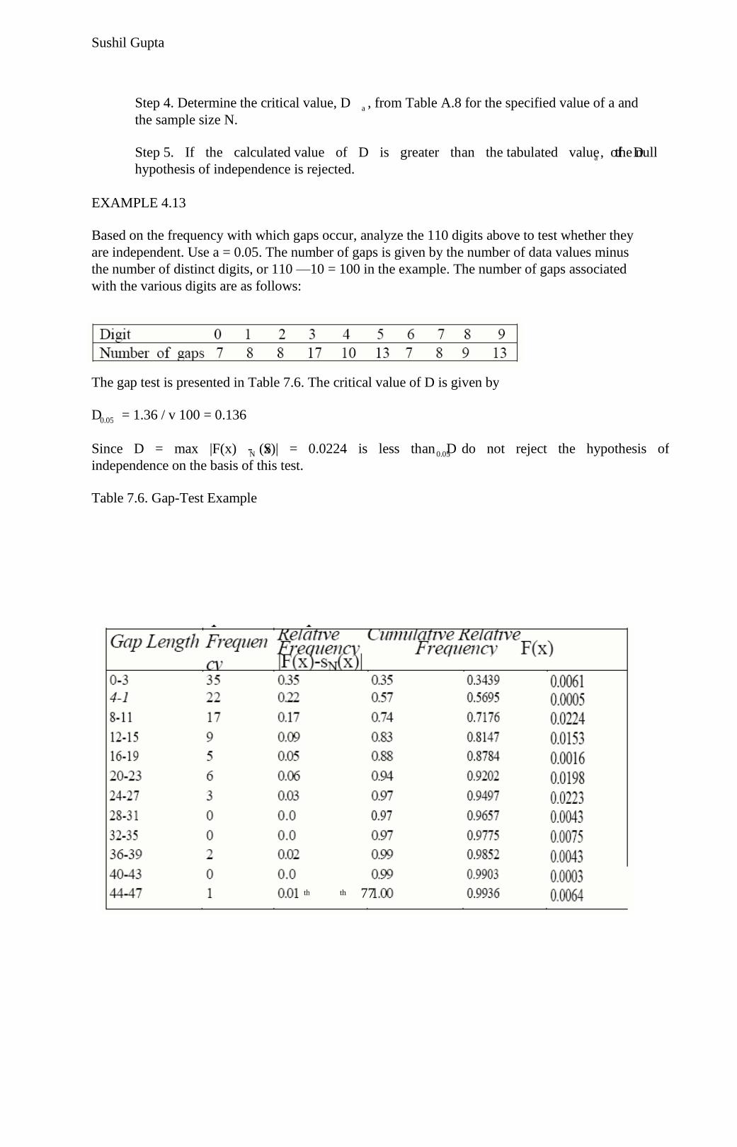
Sushil Gupta
Step 4. Determine the critical value, D , from Table A.8 for the specified value of a and a
the sample size N.
Step 5. If the calculated value of D is greater than the tabulated value of D , the null a
hypothesis of independence is rejected.
EXAMPLE 4.13
Based on the frequency with which gaps occur, analyze the 110 digits above to test whether they
are independent. Use a = 0.05. The number of gaps is given by the number of data values minus
the number of distinct digits, or 110 —10 = 100 in the example. The number of gaps associated
with the various digits are as follows:
The gap test is presented in Table 7.6. The critical value of D is given by
D = 1.36 / v 100 = 0.136 0.05
Since D = max |F(x) - S (x)| = 0.0224 is less than D do not reject the hypothesis of N 0.05
independence on the basis of this test.
Table 7.6. Gap-Test Example
77 th th
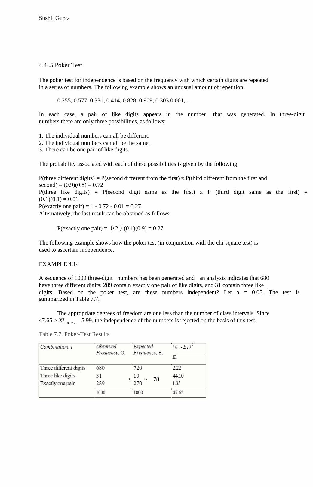
Sushil Gupta
4.4 .5 Poker Test
The poker test for independence is based on the frequency with which certain digits are repeated
in a series of numbers. The following example shows an unusual amount of repetition:
0.255, 0.577, 0.331, 0.414, 0.828, 0.909, 0.303,0.001, ...
In each case, a pair of like digits appears in the number that was generated. In three-digit
numbers there are only three possibilities, as follows:
1. The individual numbers can all be different.
2. The individual numbers can all be the same. 3. There can be one pair of like digits.
The probability associated with each of these possibilities is given by the following
P(three different digits) = P(second different from the first) x P(third different from the first and
second) = (0.9)(0.8) = 0.72
P(three like digits) = P(second digit same as the first) x P (third digit same as the first) =
(0.1)(0.1) = 0.01
P(exactly one pair) = 1 - 0.72 - 0.01 = 0.27
Alternatively, the last result can be obtained as follows:
( ) P(exactly one pair) = 2 (0.1)(0.9) = 0.27 3
The following example shows how the poker test (in conjunction with the chi-square test) is
used to ascertain independence.
EXAMPLE 4.14
A sequence of 1000 three-digit numbers has been generated and an analysis indicates that 680
have three different digits, 289 contain exactly one pair of like digits, and 31 contain three like
digits. Based on the poker test, are these numbers independent? Let a = 0.05. The test is
summarized in Table 7.7.
The appropriate degrees of freedom are one less than the number of class intervals. Since
47.65 > X 5.99. the independence of the numbers is rejected on the basis of this test. 2 0.05.2 =
Table 7.7. Poker-Test Results
78 th th

Sushil Gupta
* * * * *
79 th th
Sushil Gupta
CHAPTER – 5
RANDOM - VARIATE GENERATION
INTRODUCTION :
This chapter deals with procedures for sampling from a variety of widely
used continuous and discrete distributions. Here it is assumed that a distribution
has been completely specified, and ways are sought to generate samples from this
distribution to be used as input to a simulation model. The purpose of the chapter is
to explain and illustrate some wid ely used techniques fo r generating random
variates, n ot to give a stateof-th e-art survey of the most efficient techniques.
TECHNIQUES:
• INVERSE TRANSFORMATION TECHNIQUE
• ACCEPTANCE-REJECTION TECHNIQUE
All these techniques assume that a source of u niform (0,1) random numbers is
available R1,R2….. where each R1 has p robability density function
pdf fR(X)= 1 , 0<= X <=1
0 , otherwise
cumulative distribution fu nction
cdf fR(X)= 0 , X<0
X , 0<= X <= 1
1 , X>1
The random variables may be either discrete or continuous.
5.1 Inverse Transform Technique :
80 th th
Sushil Gupta
The inverse transform technique can be used to sample from exponential, the uniform,
the Weibull, and the triangular distributions and empirical distri-Jbutions. Additionally, it is the
underlying principle for sampling from a wide variety of discrete distributions. The technique
will be explained in detail for the exponential distribution and then applied to other distributions.
It is the most straightforward, but always the most efficient., technique computationally.
5.1.1 EXPONENTIAL DISTRIBUTION :
The exponential distribution, discussed as before has probability density function (pdf)
given by
f(X)= e , x = 0 - x
0, x < 0
and cumulative distribution function (cdf) given by
f(X) = f(t) dt = 1 – e x, x = 0 x – -8
0, x < 0
The parameter can be interpreted as the mean number of occurrences per time unit.
For example, if interarrival times Xi , X2, X3, . . . had an exponential distribution with rate , then
could be interpreted as the mean number of arrivals per time unit, or the arrival rate| Notice that for any j
E(Xi)= 1/
so that is the mean interarrival time. The goal here is to develop a procedure for generating
values X1,X2,X3, ….. which have an exponential distribution.
The inverse transform technique can be utilized, at least in principle, for any distribution. But it
is most useful when the cdf. F(x), is of such simple form that its inverse, F , can be easily
computed. A step-by-step procedure for the inverse tr ansform technique illustrated by me
exponential distribution, is as follows:
Step 1. Compute the cdf of the desired random variable X. For the exponential distribution, the
cdf is F(x) = 1 — e , x > 0.
Step 2. Set F(X) = R on the range of X. For the exponential distribution, it becomes 1 – e = R - X
on the range x >=0. Since X is a random variable (with the exponential distribution in this case),
it follows that 1 - is also a random variable, here called R. As will be shown later, R has a
uniform distribution over the interval (0,1).,
Step 3. Solve the equation F(X) = R for X in terms of R. For the exponential distribution, the
solution proceeds as follows:
81 th th
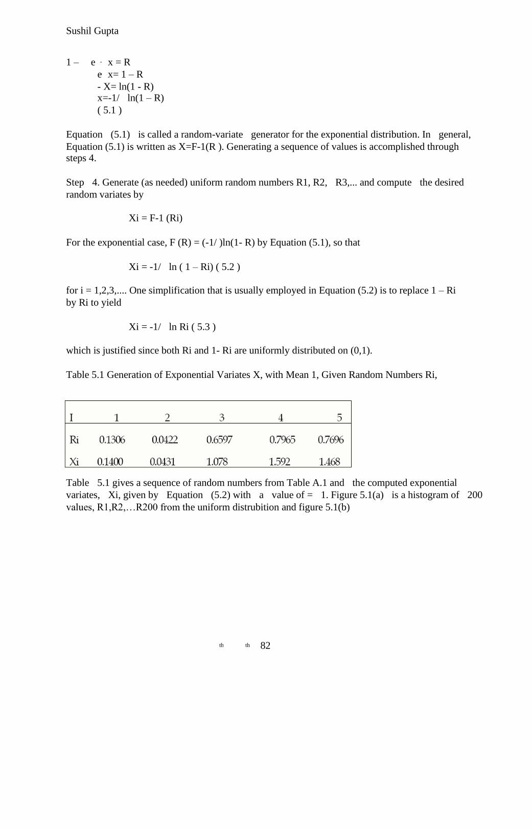
Sushil Gupta
1 – e x = R -
e x= 1 – R -
- X= ln(1 - R)
x=-1/ ln(1 – R)
( 5.1 )
Equation (5.1) is called a random-variate generator for the exponential distribution. In general,
Equation (5.1) is written as X=F-1(R ). Generating a sequence of values is accomplished through
steps 4.
Step 4. Generate (as needed) uniform random numbers R1, R2, R3,... and compute the desired
random variates by
Xi = F-1 (Ri)
For the exponential case, F (R) = (-1/ )ln(1- R) by Equation (5.1), so that
Xi = -1/ ln ( 1 – Ri) ( 5.2 )
for i = 1,2,3,.... One simplification that is usually employed in Equation (5.2) is to replace 1 – Ri
by Ri to yield
Xi = -1/ ln Ri ( 5.3 )
which is justified since both Ri and 1- Ri are uniformly distributed on (0,1).
Table 5.1 Generation of Exponential Variates X, with Mean 1, Given Random Numbers Ri,
Table 5.1 gives a sequence of random numbers from Table A.1 and the computed exponential
variates, Xi, given by Equation (5.2) with a value of = 1. Figure 5.1(a) is a histogram of 200
values, R1,R2,…R200 from the uniform distrubition and figure 5.1(b)
82 th th
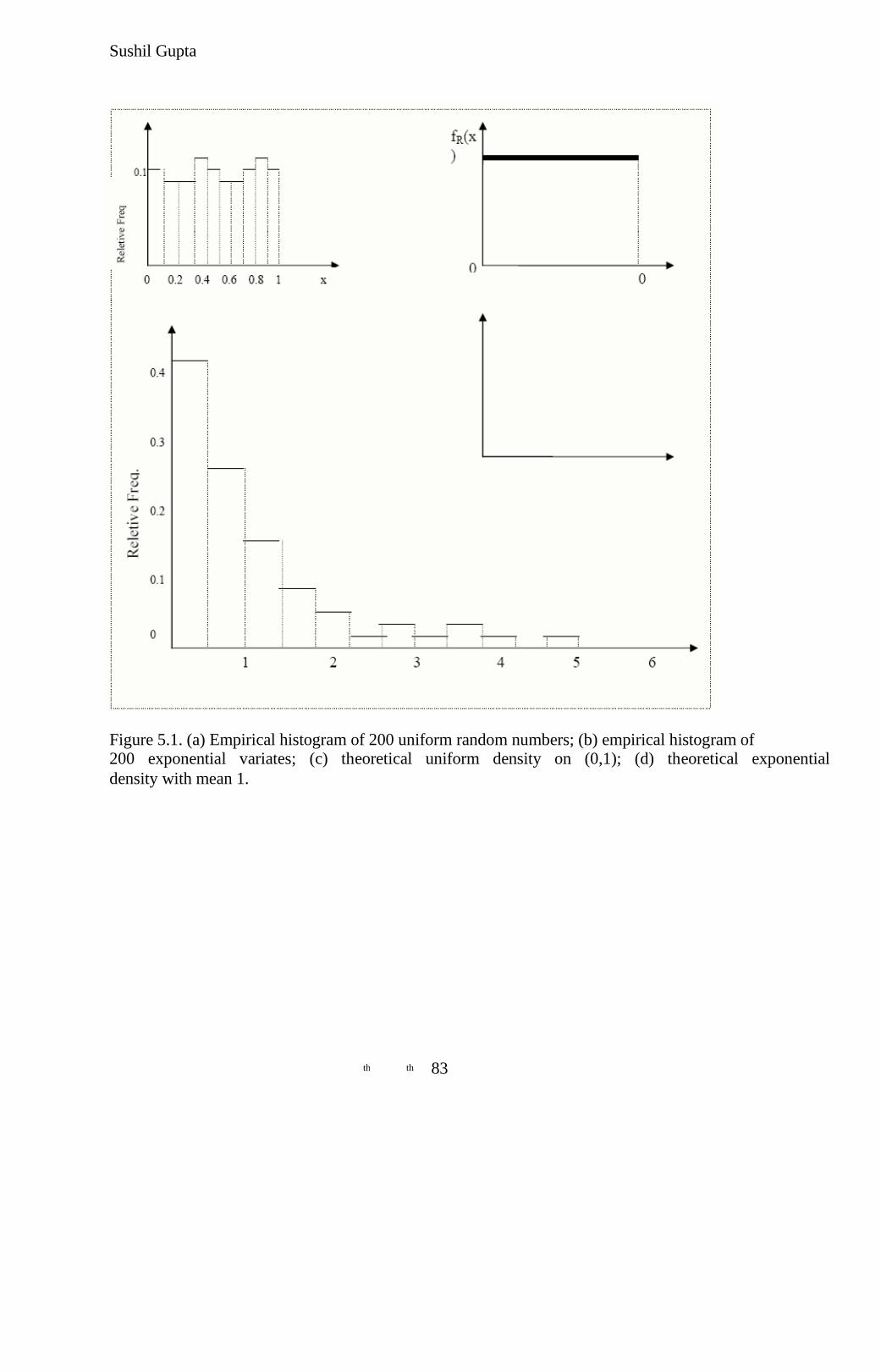
Sushil Gupta
Figure 5.1. (a) Empirical histogram of 200 uniform random numbers; (b) empirical histogram of
200 exponential variates; (c) theoretical uniform density on (0,1); (d) theoretical exponential
density with mean 1.
83 th th
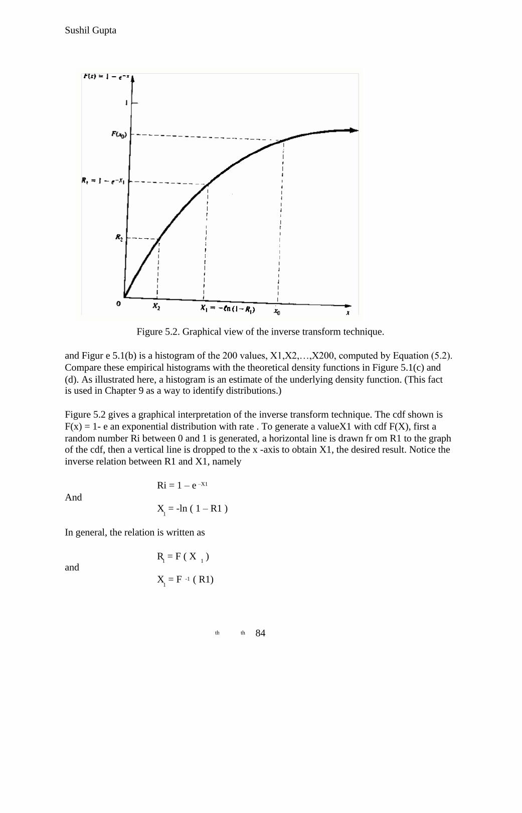
Sushil Gupta
Figure 5.2. Graphical view of the inverse transform technique.
and Figur e 5.1(b) is a histogram of the 200 values, X1,X2,…,X200, computed by Equation (5.2).
Compare these empirical histograms with the theoretical density functions in Figure 5.1(c) and
(d). As illustrated here, a histogram is an estimate of the underlying density function. (This fact is used in Chapter 9 as a way to identify distributions.)
Figure 5.2 gives a graphical interpretation of the inverse transform technique. The cdf shown is
F(x) = 1- e an exponential distribution with rate . To generate a valueX1 with cdf F(X), first a
random number Ri between 0 and 1 is generated, a horizontal line is drawn fr om R1 to the graph
of the cdf, then a vertical line is dropped to the x -axis to obtain X1, the desired result. Notice the
inverse relation between R1 and X1, namely
Ri = 1 – e –X1
And
X = -ln ( 1 – R1 ) 1
In general, the relation is written as
R = F ( X ) 1 1
and
X = F ( R1) -1 1
84 th th
Sushil Gupta
Why does the random variable X1 generated by this pr ocedure have the desired distribution?
Pick a value JCQ and compute the cumulative probability
P(X1 < x0) = P(R1 < F(x0)) = F(X0)
To see the first equality in Equation (8.4), refer to Figure 5.2, where the fixed numbers x0 and
F(X0) are drawn on their respective axes. It can be seen that X1 < xo when and only when R1 <
F(X0). Since 0 < F(xo) < 1, the second equality in Equation (8.4) follows immediately from the
fact that R\ is uniformly distributed on (0,1). Equation (8.4) shows that the cdf of X1 is F; hence,
X1 has the desired distribution.
5.1.2 Uniform Distribution :
Consider a random variable X that is uniformly distributed on the interval [a, b]. A reasonable
guess for generating X is given by
X = a + (b - a)R (5.5)
[Recall that R is always a random number on (0,1). The pdf of X is given by
f (x) = 1/ ( b-a ), a = x = b
0, otherwise
The derivation of Equation (5..5) follows steps 1 through 3 of Section 5.1.1:
Step 1. The cdf is given by
F(x) = 0, x < a
( x – a ) / ( b –a ), a = x = b
1, x > b
Step 2. Set F(X) = (X - a)/(b -a) = R
Step 3. Solving for X in terms of R yields X = a + (b — a)R, which agrees with Equation ( 5.5).
5.1.3 Discrete Distribution
All discrete distributions can be generated using the inverse transform technique, either
numerically through a table-lookup procedure, or in some cases algebraically with the final
generation scheme in terms of a formula. Other techniques are sometimes used f or certain
distributions, such as the convolution technique for the binomial distribution. Some of these
methods are discussed in later sections. This subsection gives examples covering both empirical
distributions and two of the standard discrete distributions, the (discrete) uniform and the
geometric. Highly efficient table-lookup procedures for these and other distributions are found in
Bratley, Fox, and Schrage [1987] and Ripley [1987].
85 th th
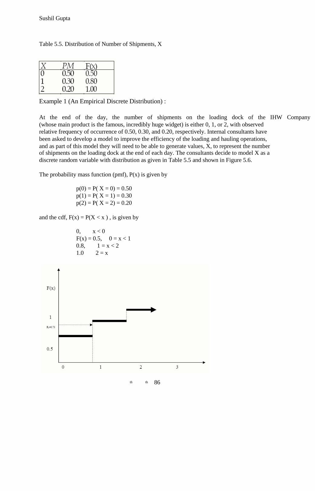
Sushil Gupta
Table 5.5. Distribution of Number of Shipments, X
Example 1 (An Empirical Discrete Distribution) :
At the end of the day, the number of shipments on the loading dock of the IHW Company
(whose main product is the famous, incredibly huge widget) is either 0, 1, or 2, with observed
relative frequency of occurrence of 0.50, 0.30, and 0.20, respectively. Internal consultants have
been asked to develop a model to improve the efficiency of the loading and hauling operations,
and as part of this model they will need to be able to generate values, X, to represent the number
of shipments on the loading dock at the end of each day. The consultants decide to model X as a
discrete random variable with distribution as given in Table 5.5 and shown in Figure 5.6.
The probability mass function (pmf), P(x) is given by
p(0) = P( X = 0) = 0.50
p(1) = P( X = 1) = 0.30
p(2) = P( X = 2) = 0.20
and the cdf, F(x) = P(X < x ) , is given by
0, x < 0
F(x) = 0.5, 0 = x < 1
0.8, 1 = x < 2
1.0 2 = x
86 th th
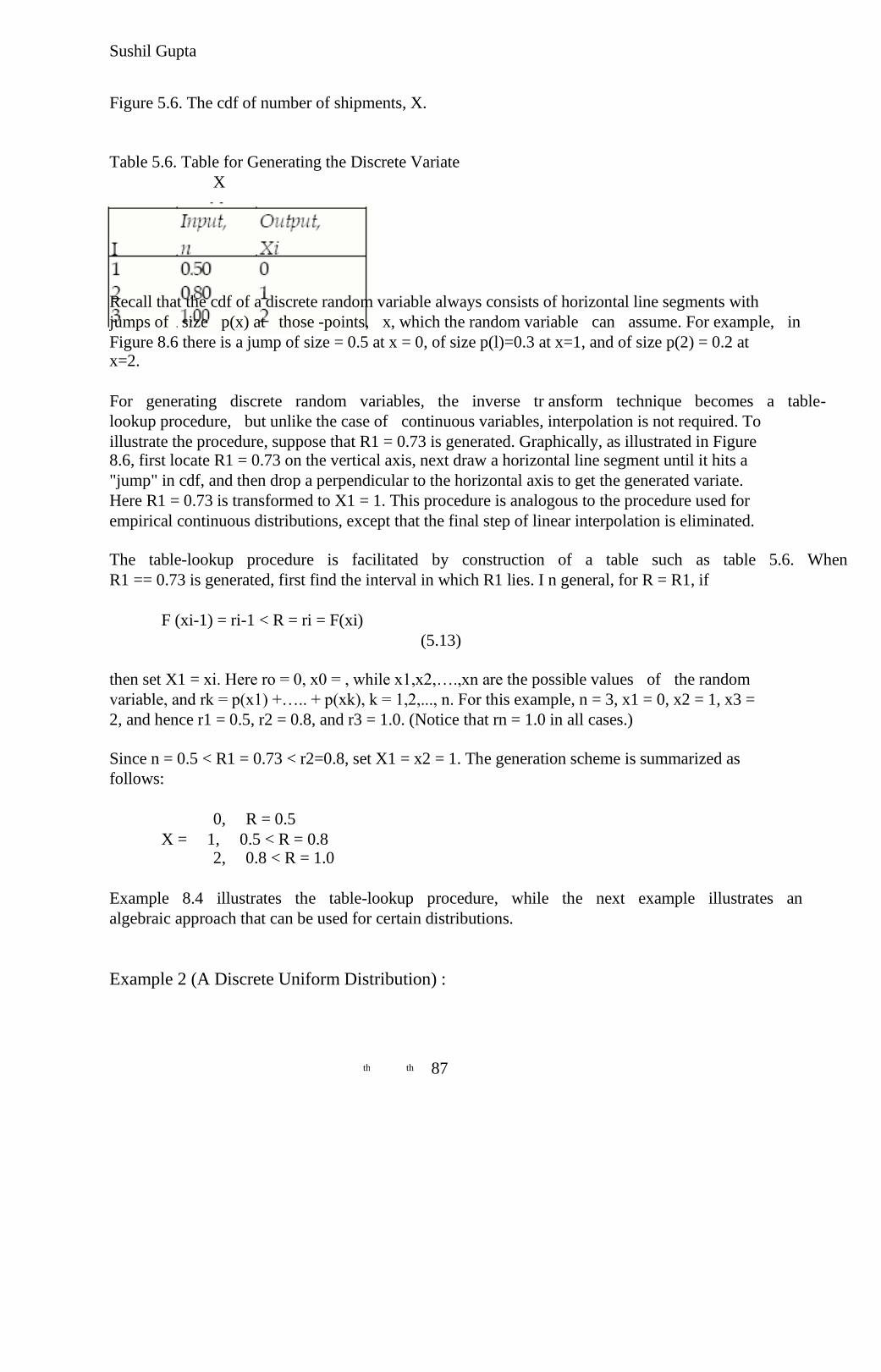
Sushil Gupta
Figure 5.6. The cdf of number of shipments, X.
Table 5.6. Table for Generating the Discrete Variate
X
Recall that the cdf of a discrete random variable always consists of horizontal line segments with
jumps of size p(x) at those -points, x, which the random variable can assume. For example, in
Figure 8.6 there is a jump of size = 0.5 at x = 0, of size p(l)=0.3 at x=1, and of size p(2) = 0.2 at x=2.
For generating discrete random variables, the inverse tr ansform technique becomes a table-
lookup procedure, but unlike the case of continuous variables, interpolation is not required. To
illustrate the procedure, suppose that R1 = 0.73 is generated. Graphically, as illustrated in Figure
8.6, first locate R1 = 0.73 on the vertical axis, next draw a horizontal line segment until it hits a
"jump" in cdf, and then drop a perpendicular to the horizontal axis to get the generated variate.
Here R1 = 0.73 is transformed to X1 = 1. This procedure is analogous to the procedure used for
empirical continuous distributions, except that the final step of linear interpolation is eliminated.
The table-lookup procedure is facilitated by construction of a table such as table 5.6. When
R1 == 0.73 is generated, first find the interval in which R1 lies. I n general, for R = R1, if
F (xi-1) = ri-1 < R = ri = F(xi)
(5.13)
then set X1 = xi. Here ro = 0, x0 = , while x1,x2,….,xn are the possible values of the random
variable, and rk = p(x1) +….. + p(xk), k = 1,2,..., n. For this example, n = 3, x1 = 0, x2 = 1, x3 =
2, and hence r1 = 0.5, r2 = 0.8, and r3 = 1.0. (Notice that rn = 1.0 in all cases.)
Since n = 0.5 < R1 = 0.73 < r2=0.8, set X1 = x2 = 1. The generation scheme is summarized as
follows:
0, R = 0.5
X = 1, 0.5 < R = 0.8
2, 0.8 < R = 1.0
Example 8.4 illustrates the table-lookup procedure, while the next example illustrates an
algebraic approach that can be used for certain distributions.
Example 2 (A Discrete Uniform Distribution) :
87 th th
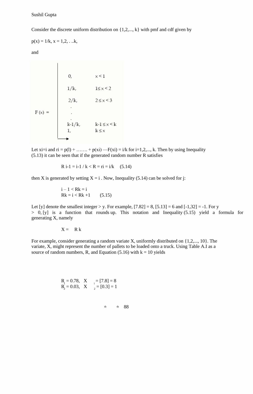
Sushil Gupta
Consider the discrete uniform distribution on {1,2,..., k} with pmf and cdf given by
p(x) = 1/k, x = 1,2, . ..k,
and
Let xi=i and ri = p(l) + ……. + p(xi) —F(xi) = i/k for i=1,2,..., k. Then by using Inequality
(5.13) it can be seen that if the generated random number R satisfies
R i-1 = i-1 / k < R = ri = i/k (5.14)
then X is generated by setting X = i . Now, Inequality (5.14) can be solved for j:
i – 1 < Rk = i
Rk = i < Rk +1 (5.15)
Let [y] denote the smallest integer > y. For example, [7.82] = 8, [5.13] = 6 and [-1,32] = -1. For y
> 0, [y] is a function that rounds up. This notation and Inequality (5.15) yield a formula for
generating X, namely
X = R k
For example, consider generating a random variate X, uniformly distributed on {1,2,..., 10}. The
variate, X, might represent the number of pallets to be loaded onto a truck. Using Table A.I as a
source of random numbers, R, and Equation (5.16) with k = 10 yields
R = 0.78, X = [7.8] = 8 1 i
R = 0.03, X = [0.3] = 1 2 2
88 th th
Sushil Gupta
R = 0.23, X = [2.3] = 3 3 3
R = 0.97, X = [9.7] = 10 4 4
The procedure discussed here can be modified to generate a discrete uniform random variate
with any range consisting of consecutive integers. Exercise 13 asks the student to devise a
procedure for one such case.
Example 3 (The Geo metric Distribution)
Consider the geometric distribution with pmf
p(x) = p ( l - p ) , x = 0,1,2,... x
where 0 < p < 1. Its cdf is given by
F(x) = p(1 – p) x j j=0
= p{1- (1- p) } / 1 – (1 – p) x+1
= 1 – ( 1 – p) x+1
for x = 0, 1, 2, ... Using the inverse transform technique [i.e., Inequality (5.13)], recall that a
geometric random variable X will assume the value x whenever
F(x - 1) = 1 - (1 –p) x < R < 1 - (1 – p) x+1 = F(x) (5.19)
where R is a generated random number assumed 0 < R <1. Solving Inequality (5.19) for x
proceeds as follows:
(1-p) = 1 – R < ( 1 – p ) x+1 x
( x + 1)ln (1 – p) = ln (1 – R ) < x ln(1 – p)
But 1 – p < 1 implies that ln(1-p) < 0. so that
Ln ( 1 –R ) / ln ( 1 –p ) -1 = x < ln(1 – R) / ln (1 – p) (5.20)
Thus, X=x for that integer value of x satisfying Inequality (5.20) or in brief using the round-up
function .
X = ln (1 – R ) / ln (1 – p ) – 1 ( 5.21)
Since p is a fixed parameter, let = —l/ n(l — p). Then > 0 and, by Equation (5.21), X = [ - ]. By
Equation (5.1), is an exponentially distributed random variable with mean , so that one way of
generating a geometr ic variate with parameter p is to generate (by any method) an exponential
variate with parameter, subtract one, and round up.Occasionally, a geometric variate X is needed
which can assume values {q, q + 1, q + 2,...} with pmf p(x) = p(1 - p) (x = q, q +1,...). Such a
variate, X can be generated,
using Equation (5.21), by
X = q + ln (1-R)/ ln(1 – p) -1
One of the most common cases is q = 1.
89 th th
Sushil Gupta
5.2 Acceptance-Rejection Technique :
Suppose that an analyst needed to devise a method for generating random variates, X, uniformly
distributed between . and 1. One way to proceed would be to follow these steps:
Step1 : Generate a random number R.
Step 2a.: If R > 1/4, accept X = /?, then go to step 3.
Step 2b.: If R < 1/4, reject /?, and return to step 1.
Step 3.: If another uniform random variate on [1/4,1] is needed, repeat the procedure
beginning at step 1. If not, stop.
Each time step 1 is executed, a new random number R must be generated. Step 2a is an
―acceptance‖ and step 2b is a "rejection" in this acceptancerejection technique. To summarize the
technique, random variates (R) with some distribution (here uniform on [0,1]) are generated until
some condition (R > 1/4) is satisfied. When the condition is finally satisfied, the desired random
variate, X (here uniform on [1/4,1]), can be computed (X = R). This procedure can be shown to
be correct by recognizing that the accepted values of R are conditioned values; that is, R itself
does not have the desired distribution, but R conditioned on the event {R > 1/4} does have the
desired distribution.
To show this, take 1/4 < a < b < 1; then
P ( a < R = b | . = R = 1 ) = P (a < R = b ) / P ( . = R = 1 ) = b – a / 3/4 (5.28)
which is the correct probability for a uniform distribution on [1/4, 1]. Equation (5.28) says that
the probability distribution of /?, given that R is between 1/4 and 1 (all other values of R are
thrown out), is the desired distribution. Therefore, if 1/4 < R < 1, set X = R.
5.2 .1 Poisson Distribution :
A Poisson random variable, N, with mean a > 0 has pmf
p(n) = P( N = n) = e / n! , n = 0,1,2,……. - n
but more important, N can be interpreted as the number of arrivals from a Poisson arrival process
in one unit of time. Recall that the inter- arrival times, A1, A2,... of successive customers are
exponentially distr ibuted with rate a (i.e., a is the mean number of arrivals per unit time); in
addition, an exponential variate can be generated by Equation (5.3). Thu/there is a relationship
between the (discrete) Poisson distribution and the (continuous) exponential distribution, namely
N = n (5.29)
if and only if
90 th th
Sushil Gupta
A1 + A2 + …………+ An = 1 < A1 + ….. + An + An+1 (5.30)
Equation (5.29)/N = n, says there were exactly n arrivals during one unit of time; but relation
(8.30) says that the nth arrival occurred before time 1 while the (n + l)st arrival occurred after
time l) Clearly, these two statements are equivalent. Proceed now by generating exponential
interarrival times until some arrival, say n + 1, occurs after time 1; then set N = n.
For efficient generation purposes, relation (5.30) is usually simplified by first using Equation
(5.3), Ai= (—1/ )ln Ri, to obtain
– 1/ ln Ri = 1 < -1/ ln Ri n n+1 i=1 i=1
Next multiply through by reverses the sign of the inequality, and use the fact that a sum of
logarithms is the logarithm of a product, to get
ln Ri = ln Ri = - > ln Ri = ln Ri n n n+1 n+1 i=1 i=1 i=1 i=1
Finally, use the relation elnx=x for any number x to obtain
Ri = e > Ri ( 8.31) n - n+1 i=1 i=1
which is equivalent to relation (8.30).The procedure for generating a Poisson random variate, N,
is given by the following steps:
Step 1. Set n = 0, P = 1.
Step 2. Generate a random number R +i and replace P by P •R +i. n n
Step 3. If P < e , then accept N = n. Otherwise, reject the current n, \ increase n -0
by one, and return to step 2.
Notice that upon completion of step 2, P is equal to the rightmost expression in relation
(5.31). The basic idea of a rejection technique is again exhibited; if P > e in step 3, then n is ~a
rejected and the generation process must proceed through at least one more trial.
How many random numbers will be required, on the average to generate one poisson
variate, N? if N=n, then n+1 random numbers are r equired so the average number is given by
E(N+1) = +1
Which is quite large if the mean , alpha, of the poisson distribution is large.
Example 4 :
91 th th
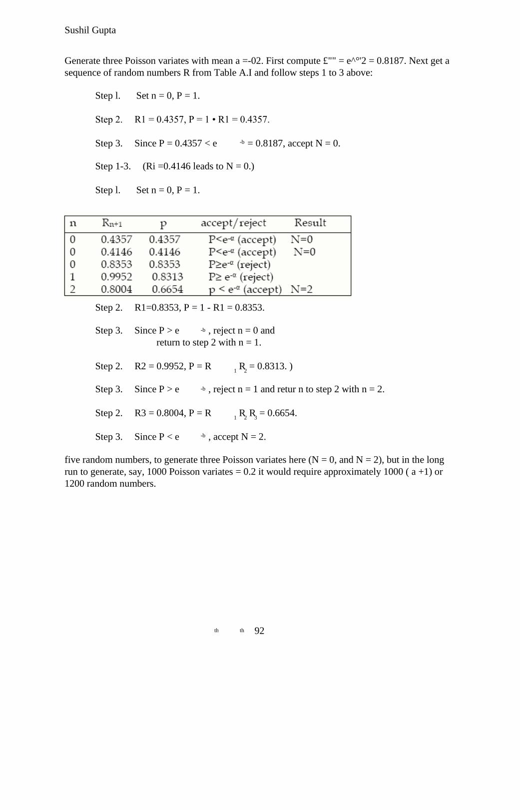
Sushil Gupta
Generate three Poisson variates with mean a =-02. First compute £"" = e^°'2 = 0.8187. Next get a
sequence of random numbers R from Table A.I and follow steps 1 to 3 above:
Step l. Set n = 0, P = 1.
Step 2. R1 = 0.4357, P = 1 • R1 = 0.4357.
Step 3. Since P = 0.4357 < e = 0.8187, accept N = 0. -b
Step 1-3. (Ri =0.4146 leads to N = 0.)
Step l. Set n = 0, P = 1.
Step 2. R1=0.8353, P = 1 - R1 = 0.8353.
Step 3. Since P > e , reject n = 0 and -b
return to step 2 with n = 1.
Step 2. R2 = 0.9952, P = R R = 0.8313. ) 1 2
Step 3. Since P > e , reject n = 1 and retur n to step 2 with n = 2. -b
Step 2. R3 = 0.8004, P = R R R = 0.6654. 1 2 3
Step 3. Since P < e , accept N = 2. -b
five random numbers, to generate three Poisson variates here (N = 0, and N = 2), but in the long
run to generate, say, 1000 Poisson variates = 0.2 it would require approximately 1000 ( a +1) or
1200 random numbers.
92 th th
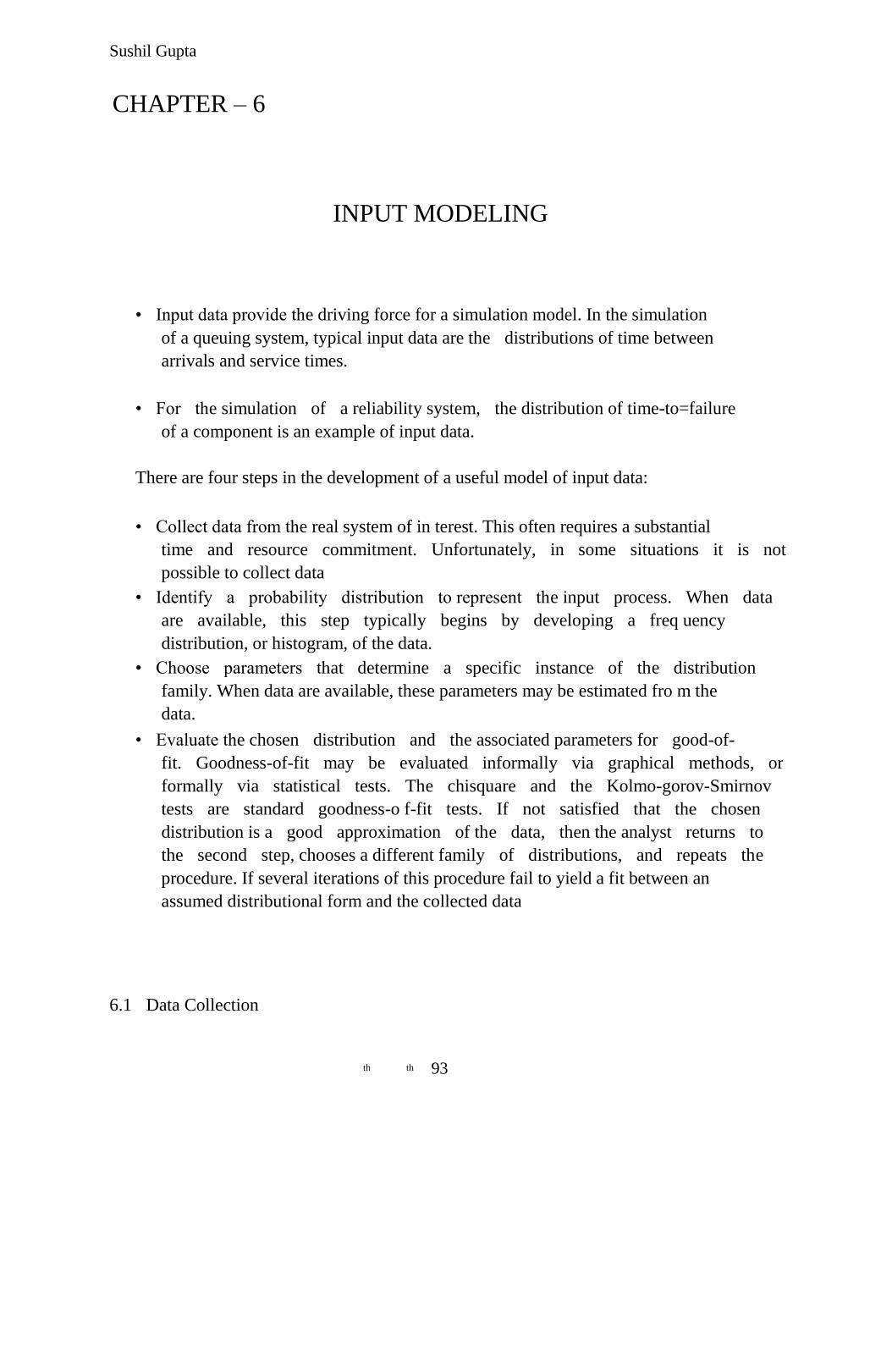
Sushil Gupta
CHAPTER – 6
INPUT MODELING
• Input data provide the driving force for a simulation model. In the simulation
of a queuing system, typical input data are the distributions of time between
arrivals and service times.
• For the simulation of a reliability system, the distribution of time-to=failure
of a component is an example of input data.
There are four steps in the development of a useful model of input data:
• Collect data from the real system of in terest. This often requires a substantial
time and resource commitment. Unfortunately, in some situations it is not
possible to collect data
• Identify a probability distribution to represent the input process. When data
are available, this step typically begins by developing a freq uency
distribution, or histogram, of the data.
• Choose parameters that determine a specific instance of the distribution
family. When data are available, these parameters may be estimated fro m the
data.
• Evaluate the chosen distribution and the associated parameters for good-of-
fit. Goodness-of-fit may be evaluated informally via graphical methods, or
formally via statistical tests. The chisquare and the Kolmo-gorov-Smirnov
tests are standard goodness-o f-fit tests. If not satisfied that the chosen
distribution is a good approximation of the data, then the analyst returns to
the second step, chooses a different family of distributions, and repeats the
procedure. If several iterations of this procedure fail to yield a fit between an
assumed distributional form and the collected data
6.1 Data Collection
93 th th
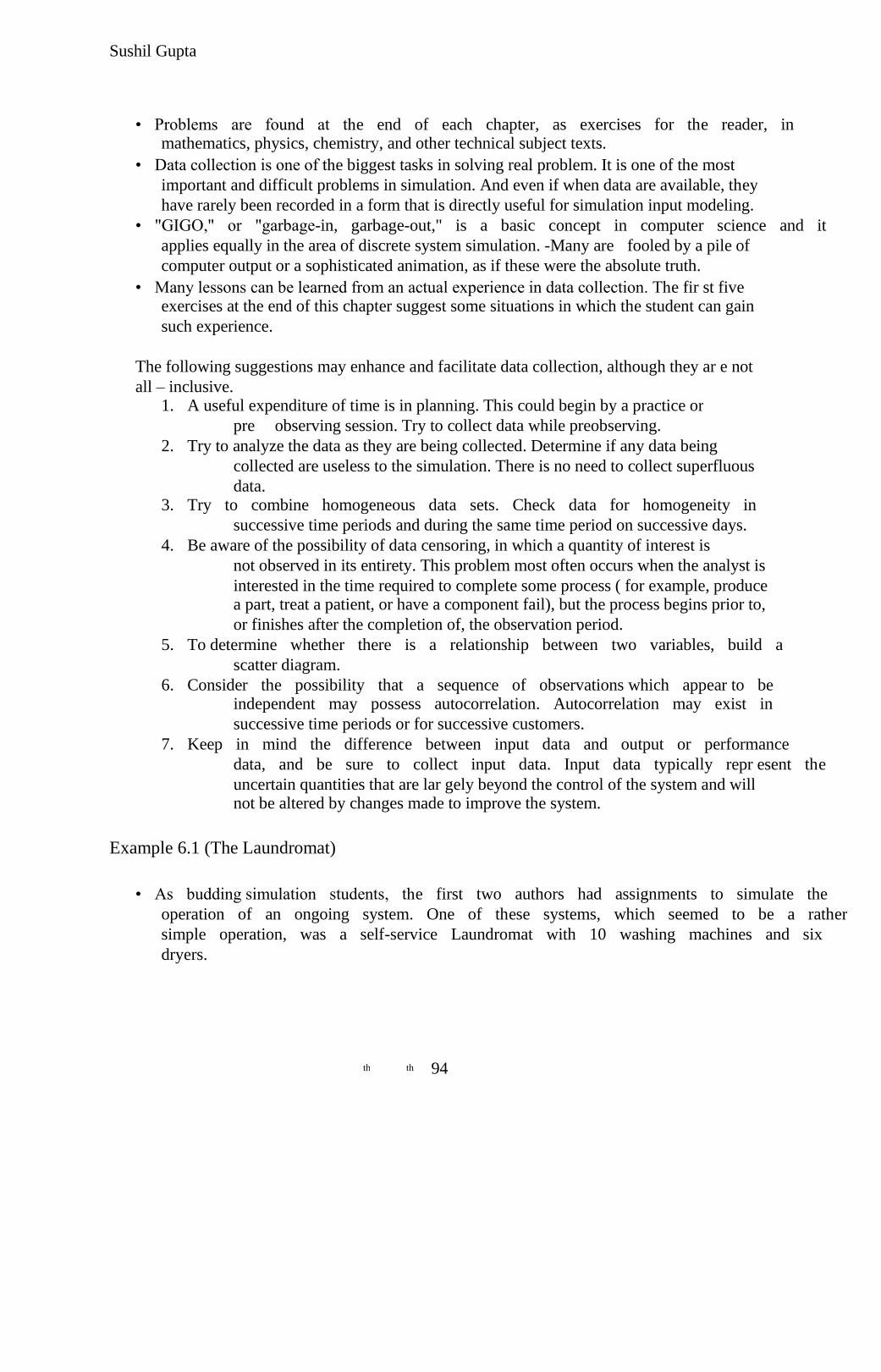
Sushil Gupta
• Problems are found at the end of each chapter, as exercises for the reader, in
mathematics, physics, chemistry, and other technical subject texts.
• Data collection is one of the biggest tasks in solving real problem. It is one of the most
important and difficult problems in simulation. And even if when data are available, they
have rarely been recorded in a form that is directly useful for simulation input modeling.
• "GIGO," or "garbage-in, garbage-out," is a basic concept in computer science and it
applies equally in the area of discrete system simulation. -Many are fooled by a pile of
computer output or a sophisticated animation, as if these were the absolute truth.
• Many lessons can be learned from an actual experience in data collection. The fir st five
exercises at the end of this chapter suggest some situations in which the student can gain
such experience.
The following suggestions may enhance and facilitate data collection, although they ar e not
all – inclusive. 1. A useful expenditure of time is in planning. This could begin by a practice or
pre observing session. Try to collect data while preobserving.
2. Try to analyze the data as they are being collected. Determine if any data being
collected are useless to the simulation. There is no need to collect superfluous
data. 3. Try to combine homogeneous data sets. Check data for homogeneity in
successive time periods and during the same time period on successive days.
4. Be aware of the possibility of data censoring, in which a quantity of interest is
not observed in its entirety. This problem most often occurs when the analyst is
interested in the time required to complete some process ( for example, produce
a part, treat a patient, or have a component fail), but the process begins prior to,
or finishes after the completion of, the observation period.
5. To determine whether there is a relationship between two variables, build a
scatter diagram.
6. Consider the possibility that a sequence of observations which appear to be
independent may possess autocorrelation. Autocorrelation may exist in
successive time periods or for successive customers.
7. Keep in mind the difference between input data and output or performance
data, and be sure to collect input data. Input data typically repr esent the
uncertain quantities that are lar gely beyond the control of the system and will not be altered by changes made to improve the system.
Example 6.1 (The Laundromat)
• As budding simulation students, the first two authors had assignments to simulate the
operation of an ongoing system. One of these systems, which seemed to be a rather
simple operation, was a self-service Laundromat with 10 washing machines and six
dryers.
94 th th
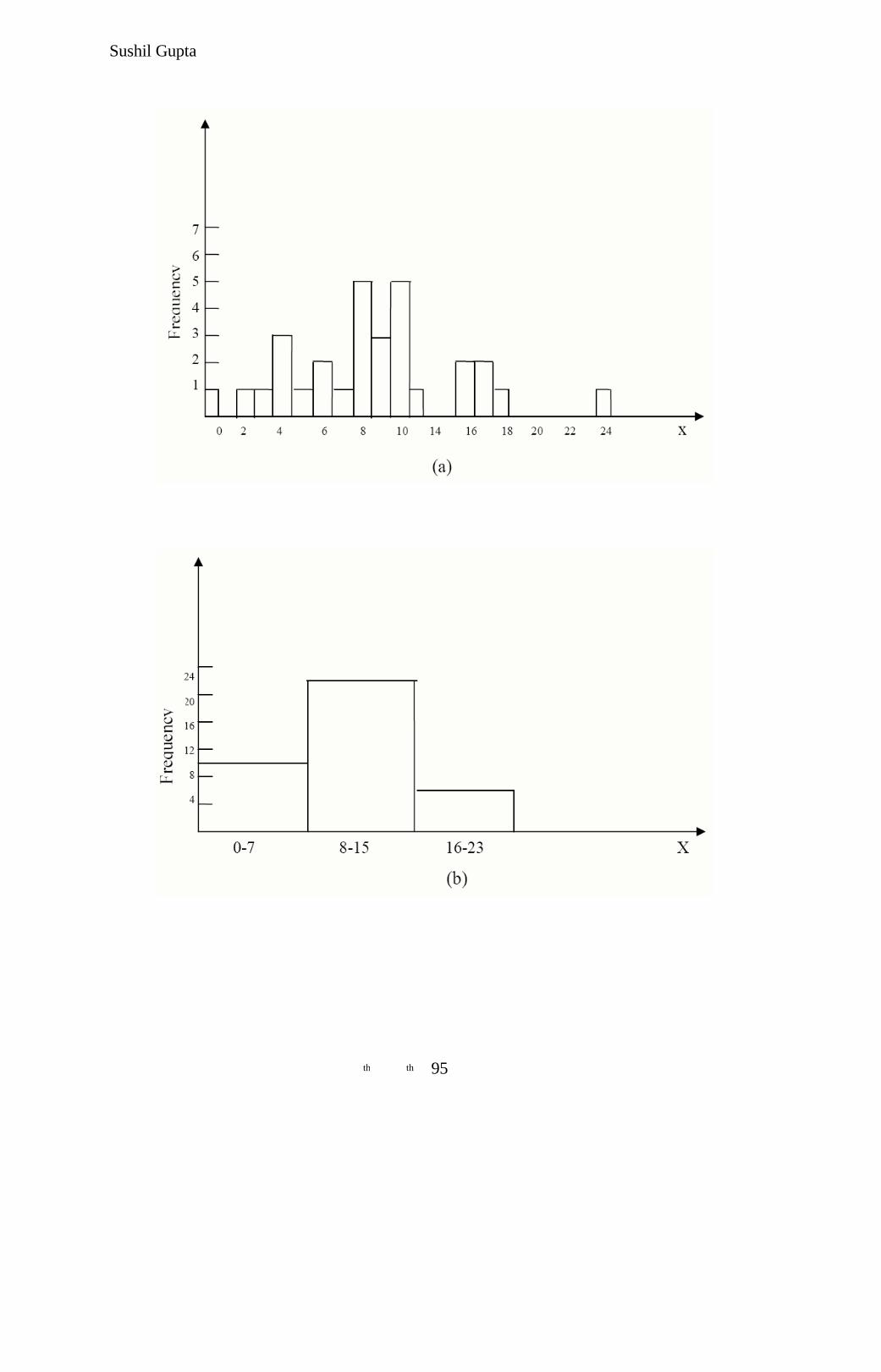
Sushil Gupta
95 th th

Sushil Gupta
Fig 6.1 Ragged, coarse, and appropriate histogram :
(a) original data- too ragged; (b) combining adjacent cells – too coarse;
(c) combining adjacent cells – appropriate
6.2 Identifying the Distribution with Data.
• In this section we discuss methods for selecting families of input distributions when data
are available.
6.2 .1 Histogram
• A frequency distribution or histogram is useful in identifying the shape of a distribution.
A histogram is constructed as follows:
1. Divide the range of the data into intervals (intervals are usually of equal width;
however, unequal widths however, unequal width may be used if the heights of the
frequencies are adjusted).
2. Label the horizontal axis to conform to the intervals selected.
3. Determine the frequency of occurrences within each interval.
4. Label the vertical axis so that the total occurrences can be plotted for each interval.
5. Plot the frequencies on the vertical axis.
• If the intervals are too wide, the histogram will be coarse, or blocky, and its shape and
other details will not show well. If the intervals are too narrow, the histogram will be
ragged and will not smooth the data.
• The histogram for continuous data corresponds to the probability density function of a
theoretical distribution.
96 th th

Sushil Gupta
Example 6.2 : The number of vehicles arriving at the northwest corner of an intersection in a 5
min period between 7 A.M. and 7:05 A.M. was monitored for five workdays over a 20-week
period. Table shows the resulting data. The first entry in the table indicates that there were 12:5
min periods during which zero vehicles arrived, 10 periods during which one vehicles arrived,
and so on,
Table 6:1 Number of Arrivals in a 5 Minute period
Fig 6.2 Histogram of number of arrivals per period.
97 th th
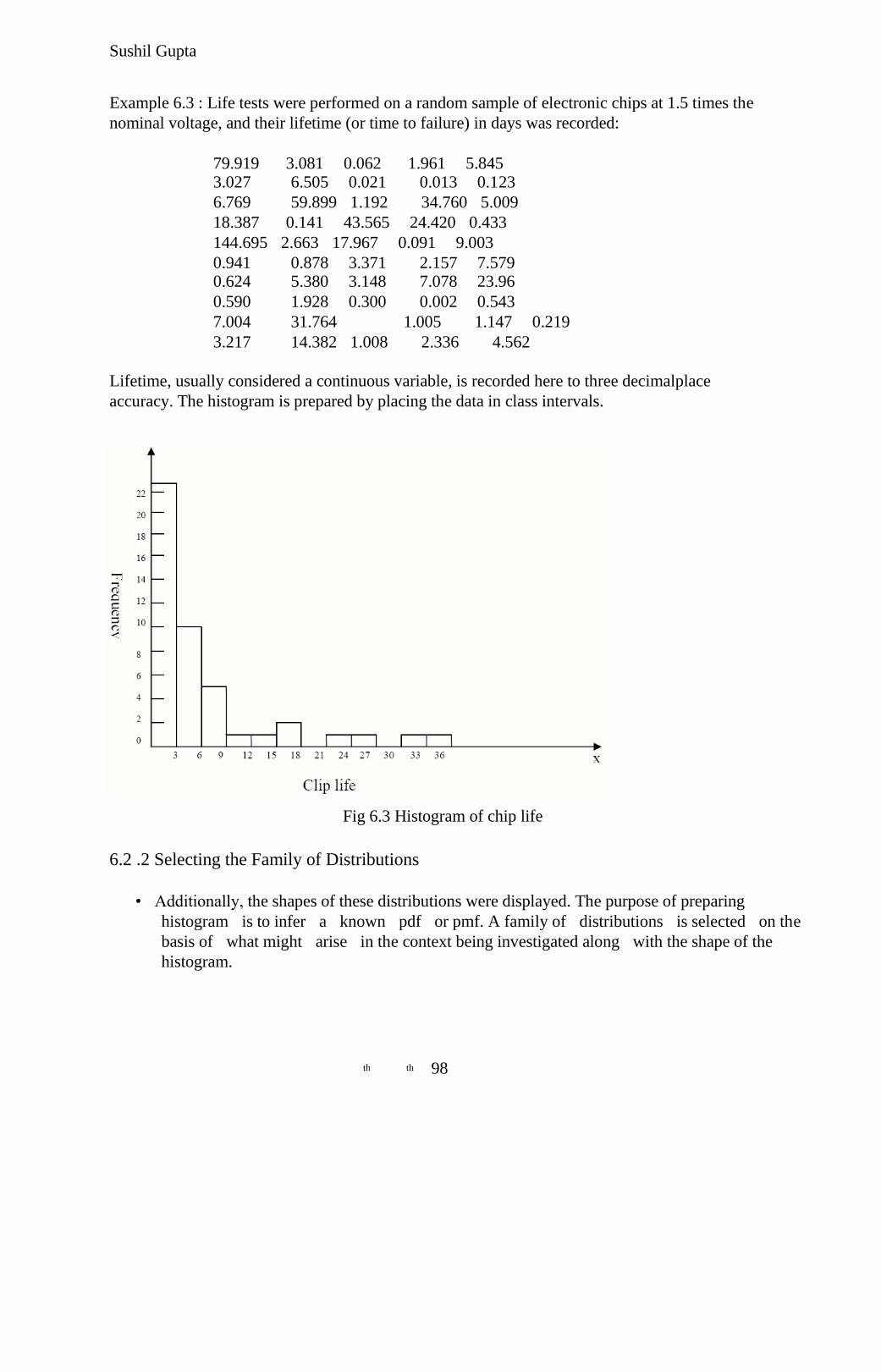
Sushil Gupta
Example 6.3 : Life tests were performed on a random sample of electronic chips at 1.5 times the
nominal voltage, and their lifetime (or time to failure) in days was recorded:
79.919 3.081 0.062 1.961 5.845
3.027 6.505 0.021 0.013 0.123
6.769 59.899 1.192 34.760 5.009
18.387 0.141 43.565 24.420 0.433
144.695 2.663 17.967 0.091 9.003
0.941 0.878 3.371 2.157 7.579
0.624 5.380 3.148 7.078 23.96
0.590 1.928 0.300 0.002 0.543
7.004 31.764 1.005 1.147 0.219
3.217 14.382 1.008 2.336 4.562
Lifetime, usually considered a continuous variable, is recorded here to three decimalplace
accuracy. The histogram is prepared by placing the data in class intervals.
Fig 6.3 Histogram of chip life
6.2 .2 Selecting the Family of Distributions
• Additionally, the shapes of these distributions were displayed. The purpose of preparing
histogram is to infer a known pdf or pmf. A family of distributions is selected on the
basis of what might arise in the context being investigated along with the shape of the
histogram.
98 th th
Sushil Gupta
• Thus, if interarrival-time data have been collected, and the histogram has a shape similar
to the pdf in Figure 5.9.the assumption of an exponential distribution would be warranted.
• Similarly, if measurements of weights of pallets of freight are being made, and the
histogram appears symmetric about the mean with a shape like that shown in Fig 5.12,
the assumption of a normal distribution would be warranted.
• The exponential, normal, and Poisson distributions are frequently encountered and are
not difficult to analyze from a computational standpoint. Although more difficult to
analyze, the gamma and Weibull distributions provide array of shapes, and should not be
overlooked when modeling an underlying probabilistic process. Perhaps an exponential distribution was assumed, but it was found not to fit the data. The next step would be to
examine where the lack of fit occurred.
• If the lack of fit was in one of the tails of the distribution, perhaps a gamma or Weibull distribution would more adequately fit the data.
• Literally hundreds of probability distributions have been created, many with some
specific physical process in mind. One aid to selecting distributions is to use the physical
basis of the distributions as a guide. Here are some examples:
Binomial : Models the number of successes in n trials, when the trials are independent with
common success probability, p; for example, the number of defective computer chips found in a
lot of n chips.
Negative Binomial (includes the geometric distribution) : Models the number of trials
required to achieve k successes; for example, the number of computer chips that we must inspect
to find 4 defective chips.
Poisson : Models the number of independent events that occur in a fixed amount of time or
space: for example, the number of customers that arrive to a store during 1 hour, or the number
of defects found in 30 square meters of sheet metal.
Normal : Models the distribution of a process that can be thought of as the sum of a number of
component processes; for example, the time to assemble a product which is the sum of the times
required for each assembly operation. Notice that the normal distribution admits negative values,
which may be-impossible for process times.
Lognormal : Models the distribution of a process that can be thought of as the product of
(meaning to multiply together) a number of component processes; for example, the rate of return
on an investment, when interest is compounded, is the product of the returns for a number of
periods.
Exponential : Models the time between independent events, or a process time which is
memoryless (knowing how much time has passed gives no information about how much
99 th th
Sushil Gupta
additional time will pass before the process is complete); for example, the times between the
arrivals of a large number of customers who act independently of each other.
The exponential is a highly variable distribution and is sometimes overused because it
often leads to mathematically tractable models. Recall that, if the time between events is
exponentially distributed, then the number of events in a fixed period of time is Poisson.
Gamma : An extremely flexible distribution used to model nonnegative random variables. The
gamma can be shifted away from 0 by adding a constant.
Beta : An extremely flexible distribution used to model bounded (fixed upper and lower limits)
random variables. The beta can be shifted away from 0 by adding a constant and can have a
larger range than [0,1] by multiplying by a constant.
Erlang : Models processes that can be viewed as the sum of several exponentially distributed
processes; for example, a computer network fails when a computer and two backup computers
fail, and each has a time to failure that is exponentially distributed. The Erlang is a special case
of the gamma. Weibull : Models the time to failure for components; for example, the time to failure for a disk
drive. The exponential is a special case of the Weibull.
Discrete or Continuous Uniform Models complete uncertainty , since all outcomes are equally
likely. This distribution is often overused when there are no data.
Triangular Models a process when only the rninimum, most-likely, and maximum values of the
distribution are known; for example, the minimum, most- likely, and maximum time required to
test a product.
Empirical Resamples from the actual data collected; often used when no theoretical distribution
seems appropriate.
• Do not ignore physical characteristics of the process when selecting distributions. Is the
process naturally discrete or continuous valued? Is it bounded or is there no natural
bound? This knowledge, which does not depend on data, can ,help narrow the family of
distributions from which to choose.
6.2 .3 Quantile-Quantile Plots
• Further, our perception of the fit depends on widths of the histogram intervals. But even
if the intervals are well chosen, grouping of data into cells makes it difficult to compare a
histogram to a continues probability density function
• If X is a random variable with cdf F, then the q-quintile of X is that y such that F(y) =
P(X < y) = q, for 0 < q < 1. When F has an invererse, we write y = F-1(q).
100 th th
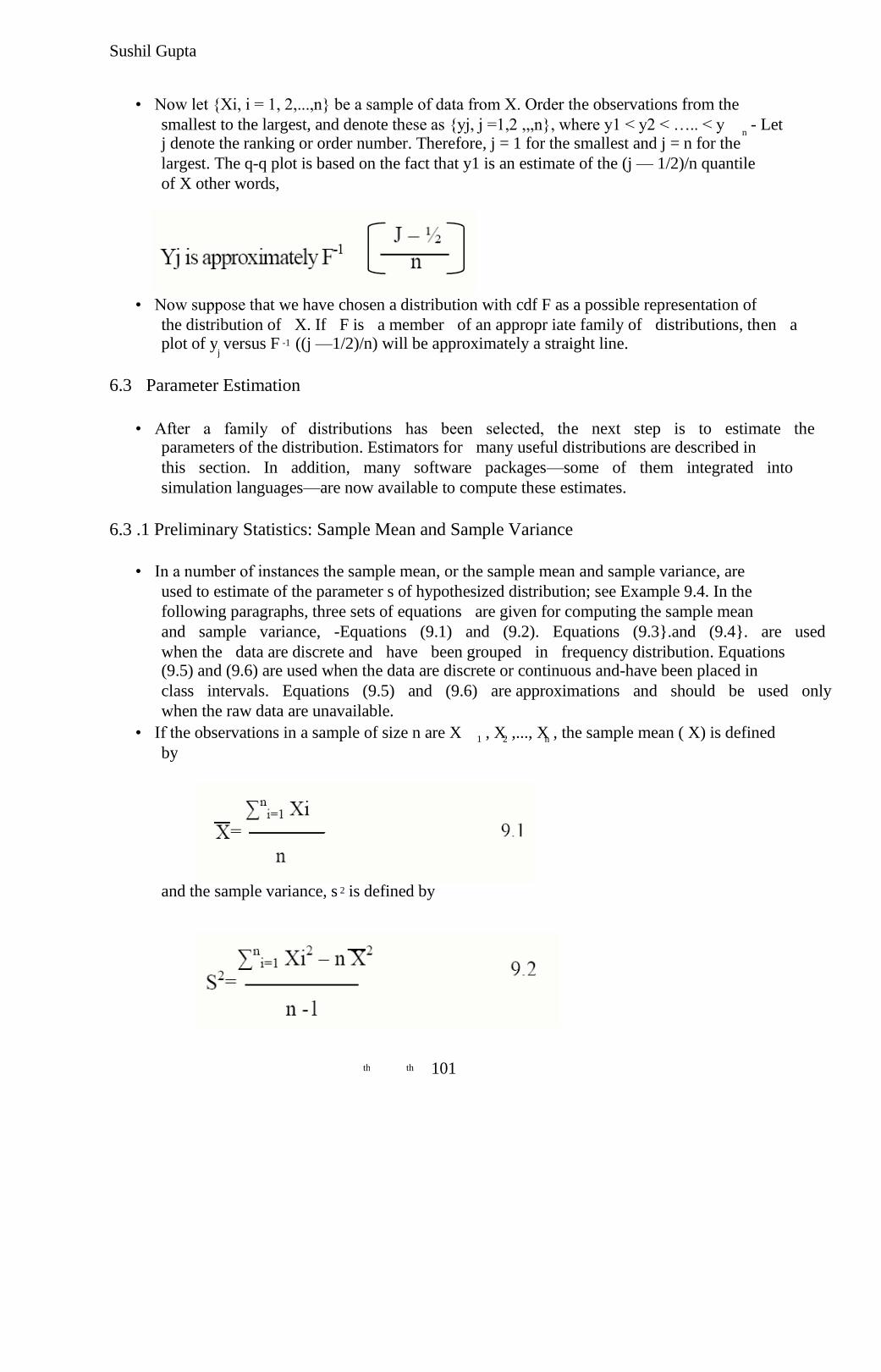
Sushil Gupta
• Now let {Xi, i = 1, 2,...,n} be a sample of data from X. Order the observations from the
smallest to the largest, and denote these as {yj, j =1,2 ,,,n}, where y1 < y2 < ….. < y - Let n
j denote the ranking or order number. Therefore, j = 1 for the smallest and j = n for the
largest. The q-q plot is based on the fact that y1 is an estimate of the (j — 1/2)/n quantile
of X other words,
• Now suppose that we have chosen a distribution with cdf F as a possible representation of
the distribution of X. If F is a member of an appropr iate family of distributions, then a
plot of y versus F ((j —1/2)/n) will be approximately a straight line. -1 j
6.3 Parameter Estimation
• After a family of distributions has been selected, the next step is to estimate the
parameters of the distribution. Estimators for many useful distributions are described in
this section. In addition, many software packages—some of them integrated into
simulation languages—are now available to compute these estimates.
6.3 .1 Preliminary Statistics: Sample Mean and Sample Variance
• In a number of instances the sample mean, or the sample mean and sample variance, are
used to estimate of the parameter s of hypothesized distribution; see Example 9.4. In the
following paragraphs, three sets of equations are given for computing the sample mean
and sample variance, -Equations (9.1) and (9.2). Equations (9.3}.and (9.4}. are used
when the data are discrete and have been grouped in frequency distribution. Equations
(9.5) and (9.6) are used when the data are discrete or continuous and-have been placed in
class intervals. Equations (9.5) and (9.6) are approximations and should be used only
when the raw data are unavailable.
• If the observations in a sample of size n are X , X ,..., X , the sample mean ( X) is defined 1 2 n
by
and the sample variance, s is defined by 2
101 th th
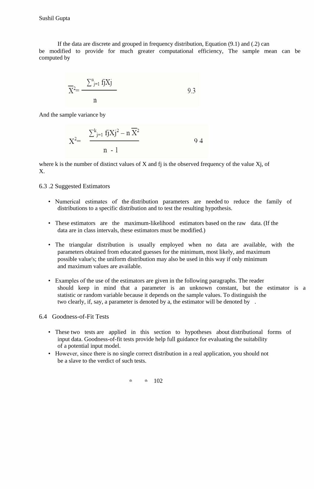
Sushil Gupta
If the data are discrete and grouped in frequency distribution, Equation (9.1) and (.2) can
be modified to provide for much greater computational efficiency, The sample mean can be
computed by
And the sample variance by
where k is the number of distinct values of X and fj is the observed frequency of the value Xj, of
X.
6.3 .2 Suggested Estimators
• Numerical estimates of the distribution parameters are needed to reduce the family of
distributions to a specific distribution and to test the resulting hypothesis.
• These estimators are the maximum-likelihood estimators based on the raw data. (If the
data are in class intervals, these estimators must be modified.)
• The triangular distribution is usually employed when no data are available, with the
parameters obtained from educated guesses for the minimum, most likely, and maximum
possible value's; the uniform distribution may also be used in this way if only minimum
and maximum values are available.
• Examples of the use of the estimators are given in the following paragraphs. The reader
should keep in mind that a parameter is an unknown constant, but the estimator is a
statistic or random variable because it depends on the sample values. To distinguish the
two clearly, if, say, a parameter is denoted by a, the estimator will be denoted by .
6.4 Goodness-of-Fit Tests
• These two tests are applied in this section to hypotheses about distributional forms of
input data. Goodness-of-fit tests provide help full guidance for evaluating the suitability
of a potential input model.
• However, since there is no single correct distribution in a real application, you should not
be a slave to the verdict of such tests.
102 th th
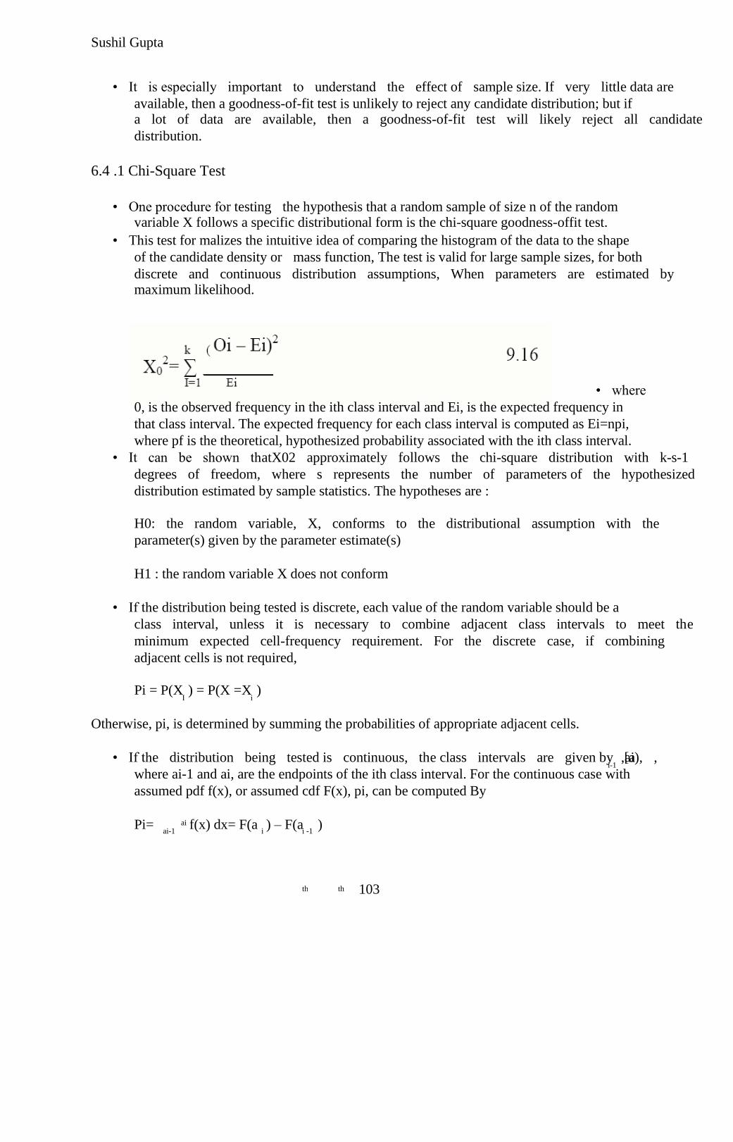
Sushil Gupta
• It is especially important to understand the effect of sample size. If very little data are
available, then a goodness-of-fit test is unlikely to reject any candidate distribution; but if
a lot of data are available, then a goodness-of-fit test will likely reject all candidate
distribution.
6.4 .1 Chi-Square Test
• One procedure for testing the hypothesis that a random sample of size n of the random
variable X follows a specific distributional form is the chi-square goodness-offit test.
• This test for malizes the intuitive idea of comparing the histogram of the data to the shape
of the candidate density or mass function, The test is valid for large sample sizes, for both
discrete and continuous distribution assumptions, When parameters are estimated by
maximum likelihood.
• where
0, is the observed frequency in the ith class interval and Ei, is the expected frequency in
that class interval. The expected frequency for each class interval is computed as Ei=npi,
where pf is the theoretical, hypothesized probability associated with the ith class interval.
• It can be shown thatX02 approximately follows the chi-square distribution with k-s-1
degrees of freedom, where s represents the number of parameters of the hypothesized
distribution estimated by sample statistics. The hypotheses are :
H0: the random variable, X, conforms to the distributional assumption with the
parameter(s) given by the parameter estimate(s)
H1 : the random variable X does not conform
• If the distribution being tested is discrete, each value of the random variable should be a
class interval, unless it is necessary to combine adjacent class intervals to meet the
minimum expected cell-frequency requirement. For the discrete case, if combining
adjacent cells is not required,
Pi = P(X ) = P(X =X ) I i
Otherwise, pi, is determined by summing the probabilities of appropriate adjacent cells.
• If the distribution being tested is continuous, the class intervals are given by [a ,ai), , i-1
where ai-1 and ai, are the endpoints of the ith class interval. For the continuous case with
assumed pdf f(x), or assumed cdf F(x), pi, can be computed By
Pi= f(x) dx= F(a ) – F(a ) ai ai-1 i i -1
103 th th
Sushil Gupta
6.4 .2 Chi-Square Test with Equal Probabilities
• If a continuous distributional assumption is being tested, class intervals that are equal in
probability rather than equal in width of interval should be used.
• Unfortunately, there is as yet no method for deter mining the; probability associated with
each interval that maximize the; power of a test o f a given size.
Ei = n p i = 5
• Substituting for p i yields n/k = 5
• and solving for k yields k = n/5
6.4 .3 Kolmogorov - Smirnov Go odness-of-Fit Test
• The chi-square goodness-of-fit test can accommodate the estimation of parameters from
the data with a resultant decrease in the degrees of freedom (one for J each parameter
estimated). The chi-square test requires that the data be placed in class intervals, and in
the case of continues distributional assumption, this grouping is arbitrary.
• Also, the distribution of the chi-square test statistic is known only approximately, and the
power of the test is sometimes rather low. As a result of these considerations, goodness-
of-fit tests, other than the chi-square, are desired.
• The Kolmogorov-Smirnov test is particularly useful when sample sizes are small and
when no parameters have been estimated from the data.
• ( Kolmogoro-Smirnov Test for Exponential Distribution)
• Suppose that 50 interarriaval times (in minutes) are collected over the following 100
minute interval (arranged in order of occurrence) :
0.44 0.53 2.04 2.74 2.00 0.30 2.54 0.52 2.02 1.89 1.53 0.21
2.80 0.04 1.35 8.32 2.34 1.95 0.10 1.42 0.46 0.07 1.09 0.76
5.55 3.93 1.07 2.26 2.88 0.67 1.12 0.26 4.57 5.37 0.12 3.19
1.63 1.46 1.08 2.06 0.85 0.83 2.44 2.11 3.15 2.90 6.58 0.64
Ho : the interarrival times are exponentially distributed
H1: the interarrival times are not exponentially distributed
• The data were collected over the interval 0 to T = 100 min. It can be shown that if the
underlying distribution of interarrival times { T1, T2, … } is exponential, the arrival
times are uniformly distributed on the interval (0,T) .
104 th th
Sushil Gupta
• The arrival times T1, T1+T2, T1+T2+T3,…..,T1+…..+T50 are obtained by adding
interarrival times.
• On a (0,1) interval, the points will be [T1/T, (T1+T2)/T,…..,(T1+….+T50)/T].
0.0044 0.0097 0.0301 0.0575 0.0775 0.0805 0.1059 0.1111 0.1313 0.1502
0.1655 0.1676 0.1956 0.1960 0.2095 0.2927 0.3161 0.3356 0.3366 0.3508
0.3553 0.3561 0.3670 0.3746 0.4300 0.4694 0.4796 0.5027 0.5315 0.5382
0.5494 0.5520 0.5977 0.6514 0.6526 0.6845 0.7008 0.7154 0.7262 0.7468
0.7553 0.7636 0.7880 0.7982 0.8206 0.8417 0.8732 0.9022 0.9680 0.9744
6.4 .4 p-Values and "Best Fits"
• To apply a goodness-of-fit test a significance level must be chosen. The traditional significance levels are 0.1,0.05, and 0.01. Prior to the availability of high-speed
computing, having a small set of standar d values made it possible to produce tables of
useful critical values. Now most statistical software computes critical values as needed,
rather than storing them in tables. Thus, if the analyst prefers a level of significance of, say, 0.07, then he or she can choose it.
• However, rather than require a prespecified significance level, many software packages
compute a p-value for the test statistic. The p-value is the significance level at which one
would just reject H0 for the given value of the test statistic. while a small pvalue suggests
a poor fit (to accept we would have to insist on almost no risk).
• The p-value can be viewed as a measure of fit, with larger values being better. This
suggests that we could fit every distribution at our disposal, compute a test statistic for
each fit, and then choose the distribution that yields the largest p-value.
• While we know of no input modeling software that implements this specific algorithm, many such packages do include a "best-fit"' option in which the software recommends an
input model to the user based on evaluating all feasible models.
• In the end some summary measure of fit, like the p-value, is used to rank the
distributions. There is nothing wrong with this, but there are several things to keep in
mind:
1. The software may know nothing about the physical basis of the data and that
information can suggest distribution families that are appropriate.
2. Recall that both the Erlang and the exponential distributions are special cases of the
gamma, while the exponential is also a special case of the more flexible Weibull.
Automated best-fit procedures tend to choose the more flexible distr ibutions (gamma
and Weibull over Erlang and exponential) because the extra flexibility allows closer
conformance to the data and a better summary measure of fit. But again, close
conformance to the data may not always lead to the most appropriate input model.
3. A summary statistic, like the p-value, is just that, a summary measure. It says little or
nothing about where the lack of fit occurs (in the body of the distribution, in the right
tail or in the left tail). A human, using graphical tools, can see where the lack of fit
occurs and decide whether or not it is important for the application at hand.
105 th th
Sushil Gupta
6.5 Selecting Input Models without Data
• Unfortunately. it is often necessary in practice to develop a simulation model for
demonstration purposes or a preliminary study—before any i data are available.) In this
case the modeler must be resourceful in choosing input models and must carefully check
the sensitivity of results to the models.
Engineering data : Often a product or process has performance ratings pro vided by the
manufacturer.
Expert option : Talk to people who are experienced with the procesws or similar processes.
Often they can provide optimistic, pessimistic and most likely times.
Physical or conventional limitations : Most real processes have physical limit on performance. Because of company policies, there may be upper limits on how long a process may take. Do not
ignore obvious limits or bound: that narrow the range of the input process.
The nature of the process It can be used to justify a particular choice even when no data are
available.
6.6 Multivariate and Time-Series Input Models
The random variables presented were considered to be independent of any other variables within
the context of the pr oblem. However, variables may be related, and if the variables appear in a
simulation model as inputs, the relationship should be determined and taken into consideration.
106 th th
Sushil Gupta
CHAPTER – 7
VERIFICATION AND VALIDATION OF
SIMULATION MODELS
• One of the most important and difficult tasks facing a model developer is the
verification and validation of the simulation model.
• It is the job of the model developer to work closely with the end users
throughout the period (development and validation to reduce this skepticism
and to increase the credibility.
• The goal of the validation process is twofold:
1: To produce a model that represents true system behavior clo sely
enough for the model to be used as a substitute for the actual system
for the purpose of experimenting with system.
2: To increase an acceptab le, level the credibility of the model ,so that
the model will be used by managers and other decision makers. |
• The verification and validation process consists of the following
components:-
1:Verification is concerned with building the model right. It is utilized
in comparison of th e conceptual model to the computer representation
that implements that conception. It asks the questions: Is the model
implemented correctly in the computer? Are the input parameters and
logical structure of the model correctly represented?
2: Validation is concerned with building the right model. It is utilized
to determine that a model is an accurate representatio n of the real
system. It is usually achieved through the calibration of the model.
107 th th
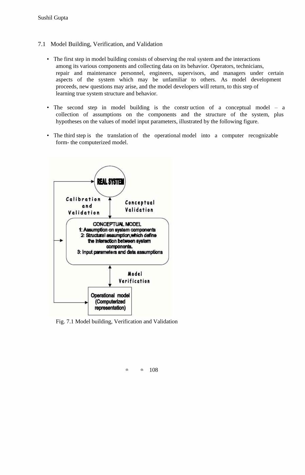
Sushil Gupta
7.1 Model Building, Verification, and Validation
• The first step in model building consists of observing the real system and the interactions
among its various components and collecting data on its behavior. Operators, technicians,
repair and maintenance personnel, engineers, supervisors, and managers under certain
aspects of the system which may be unfamiliar to others. As model development
proceeds, new questions may arise, and the model developers will return, to this step of
learning true system structure and behavior.
• The second step in model building is the constr uction of a conceptual model – a
collection of assumptions on the components and the structure of the system, plus
hypotheses on the values of model input parameters, illustrated by the following figure.
• The third step is the translation of the operational model into a computer recognizable
form- the computerized model.
Fig. 7.1 Model building, Verification and Validation
108 th th
Sushil Gupta
Verification of Simulation Models 7.2
The purpose of model verification is to assure that the conceptual model is reflected accurately in
the computerized representation.
The conceptual model quite often involves some degree of abstraction about system operations,
or some amount of simplification of actual operations.
Many common-sense suggestions can be given for use in the verification process:-
1: Have the computerized representation checked by someone other than its developer .
2: Make a flow diagram which includes each logically possible action a system can take
when an event occurs, and follow the model logic for each a for each action for each event
type.
3: Closely examine the model output for reasonableness under a variety of settings of Input
parameters.
4. Have the computerized representation print the input parameters at the end of the
Simulation to be sure that these parameter values have not been changed inadvertently.
5. Make the computerized representation of self-documenting as possible.
6. If the computerized representation is animated, verify that what is seen in the animation
jmitates the actual system.
7. The interactive run controller (IRC) or debugger is an essential component of Successful
simulation model building. Even the best of simulation analysts makes mistakes or commits
logical errors when building a model. The IRC assists in finding and correcting those errors
in the follow ways:
(a) The simulation can be monitored as it progresses.
(b) Attention can be focused on a particular line of logic or multiple lines of logic that constitute a procedure or a particular entity.
(c) Values of selected model components can be observed. When the simulation has paused,
the current value or status of variables, attributes, queues, resources, counters, etc., can be
observed.
(d) The simulation can be temporarily suspended, or paused, not only to view information
but also to reassign values or redirect entities.
8. Graphical interfaces are recommended for accomplishing verification & validation .
109 th th
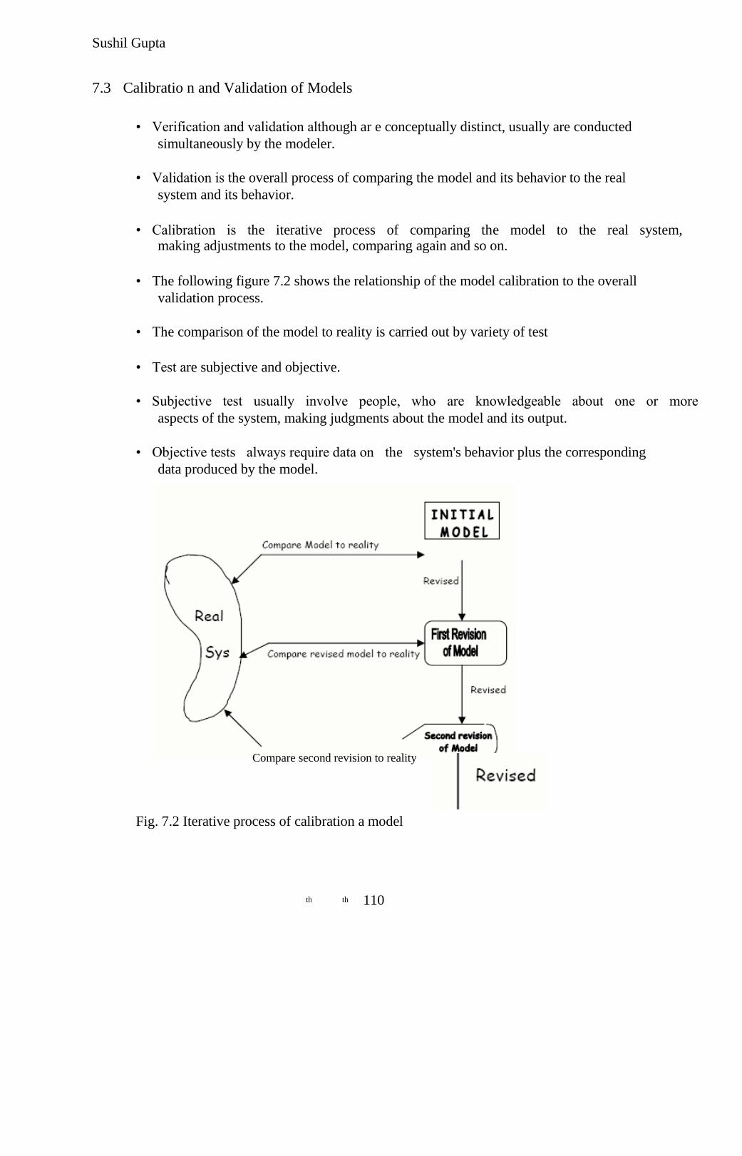
Sushil Gupta
7.3 Calibratio n and Validation of Models
• Verification and validation although ar e conceptually distinct, usually are conducted
simultaneously by the modeler.
• Validation is the overall process of comparing the model and its behavior to the real
system and its behavior.
• Calibration is the iterative process of comparing the model to the real system, making adjustments to the model, comparing again and so on.
• The following figure 7.2 shows the relationship of the model calibration to the overall
validation process.
• The comparison of the model to reality is carried out by variety of test
• Test are subjective and objective.
• Subjective test usually involve people, who are knowledgeable about one or more
aspects of the system, making judgments about the model and its output.
• Objective tests always require data on the system's behavior plus the corresponding
data produced by the model.
Compare second revision to reality
Fig. 7.2 Iterative process of calibration a model
110 th th
Sushil Gupta
• A possible criticism of the calibration phase, were it to stop at point, ie., the model
has been validated only for the one data set used; that is, the model has been "fit" to
one data set
• Validation is not an either/or proposition—no model is ever totally representative of
the system under study. In addition, each revision of the model, as in the Figure above
involves some cost, time, and effort.
As an aid in the validation process, Naylor and Finger [1967] formulated a three step
approach which has been widely followed:-
1. Build a model that has high face validity. 2. Validate model assumptions.
3. Compare the model input-output transformations to corresponding input-output
transformations for the real system.
7.3 .1 FACE VALIDITY
• The first goal of the simulation modeler is to construct a model that appears easonable
on its face to model users and others who are knowledgeable about the r eal system
being simulated.
• The users of a model should be involved in model construction from its
conceptualization to its implementation to ensure that a high degree of realism is built
into the model through reasonable assumptions regarding system structure, and
reliable data.
• Another advantage of user involvement is the increase in the models perceived
validity or credibility without which manager will not be willing to trust simulation
results as the basis for decision making.
• Sensitivity analysis can also be used to check model's face validity.
• The model user is asked if the model behaves in the expected way when one or more
input variables is changed.
• Based on experience and observations on the real system the model user and model
builder would probably have some notion at least of the direction of change in model
output when an input variable is increased or decreased.
• The model builder must attempt to choose the most critical input variables for
testing if it is too expensive or time consuming to: vary all input variables.
111 th th
Sushil Gupta
7.3 .2 Validation of Model Assumptions
*Model assumptions fall into two general classes: structural assumptions
and data assumptions.
Structural assumptions involve questions of how the system operates and usually involve
simplification and abstractions of reality.
For example, consider the customer queuing and service facility in a bank. Customers
may form one line, or there may be an individual line for each teller. If there are many
lines, customers may be served strictly on a first-come, first-served basis, or some
customers may change lines if one is moving faster. The number of tellers may be fixed
or variable. These structural assumptions should be verified by actual observation during
appropriate time periods together with discussions with managers and tellers regarding
bank policies and actual implementation of these policies.
Data assumptions should be based on the collection of reliable data and correct statistical
analysis of the data.
data were collected on:
1. Inter arrival times of customers during several 2-hour periods of peak loading
("rush-hour" traffic)
2. Inter arrival times during a slack period
3. Service times for commercial accounts
4. Service times for personal accounts.
The procedure for analyzing input data consist of three steps:-
1: Identifying the appropriate probability distribution.
2: Estimating the parameters of the hypothesized distribution .
3: Validating the assumed statistical model by goodness – of – fit test such as the chi
square test, KS test and by graphical methods.
10.3.3 Validating Input-Output Transformation:-
• In this phase of validation process the model is viewed as input –output transformation.
• That is, the model accepts the values of input parameters and transforms these inputs into
output measure of performance. It is this correspondence that is being validated.
• Instead of validating the model input-output tr ansfor mation by predicting the future ,the
modeler may use past historical data which has been served for validation purposes that
112 th th

Sushil Gupta
is, if one set has been used to develop calibrate the model, its recommended that a
separate data test be used as final validation test.
• Thus accurate ― prediction of the past‖ may replace prediction of the future for purpose of
validating the future.
• A necessary condition for input-output transformation is that some version of the system
under study exists so that the system data under at least one set of input condition can be
collected to compare to model prediction.
• If the system is in planning stage and no system operating data can be collected, complete
input-output validation is not possible.
• Validation increases modeler‘s confidence that the model of existing system is accurate.
• Changes in the computerized representation of the system, ranging from relatively minor
to relatively major include :
1: Minor changes of single numerical parameters such as speed of the machine, arrival
rate of the customer etc.
2: Minor changes of the form of a statistical distribution such as distribution of service
time or a time to failure of a machine.
3: Major changes in the logical structure of a subsystem such as change in queue
discipline for waiting-line model, or a change in the scheduling rule for a job shop model.
4: Major changes involving a different design for the new system such as computerized
inventory control system replacing a non computerized system .
If the change to the computerized representation of the system is minor such as in items one
or two these change can be carefully verified and output from new model can be accepted with
considerable confidence.
Partial validation of substantial model changes in item three and four may be possible.
7.3 .4: Input-Output Validation: Using Historical Input Da ta
When using artificially generated data as input data the modeler expects the model
produce event patterns that are compatible with, but not identical to, the event patterns that occurred in the real system during the period of data collection.
• Thus, in the bank model, artificial input data {X\n, X2n, n = 1,2, , .} for inter arrival
and service times were generated and replicates of the output data Y2 were compared
to what was observed in the real system
113 th th
Sushil Gupta
• An alternative to generating input data is to use the actual historical record, {An, Sn, n = 1,2,...}, to drive simulation model and then to compare model output to system
data.
• To implement this technique for the bank model, the data Ai, A2,..., S1 S2 would
have to be entered into the model into arrays, or stored on a file to be read as the need
arose.
• To conduct a validation test using historical input data, it is important that all input
data (An, Sn,...) and all the system response data, such as average delay(Z2), be
collected during the same time period.
• Otherwise, comparison of model responses to system responses, such as the
comparison of average delay in the model (Y2) to that in the system ( Z2), could be
misleading.
• responses (Y2 and 22) depend on the inputs (An and Sn) as well as on the structure of
the system, or model.
• Implementation of this technique could be difficult for a large system because of the
need for simultaneous data collection of all input variables and those response
variables of primary interest.
7.3 .5: Input-Output Validation: Using a Turing Test
In addition to statistical tests, or when no statistical test is readily applicable persons
knowledgeable about system behavior can be used to compare model output to system
output.
For example, suppose that five reports of system performance over five different days are
prepared, and simulation output are used to produce five "fake" reports. The 10 reports
should all be in exactly in the same format and should contain information of the type
that manager and engineer have previously seen on the system.
• The ten reports are randomly shuffled and given to the engineers, who is asked to
decide which report are fake and which are real.
• If engineer identifies substantial number of fake reports the model builder questions
the engineer and uses the information gained to improve the model.
• If the engineer cannot distinguish between fake and real reports with any consistency,
the modeler will conclude that this test provides no evidence of model inadequacy .
• This type of validation test is called as TURING TEST.
114 th th
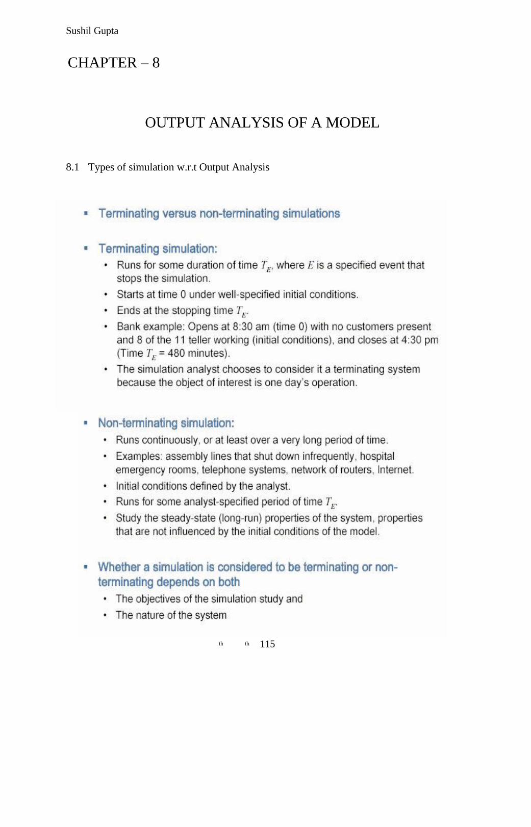
Sushil Gupta
CHAPTER – 8
OUTPUT ANALYSIS OF A MODEL
8.1 Types of simulation w.r.t Output Analysis
115 th th
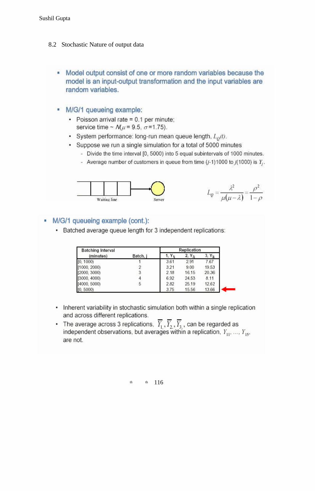
Sushil Gupta
8.2 Stochastic Nature of output data
116 th th
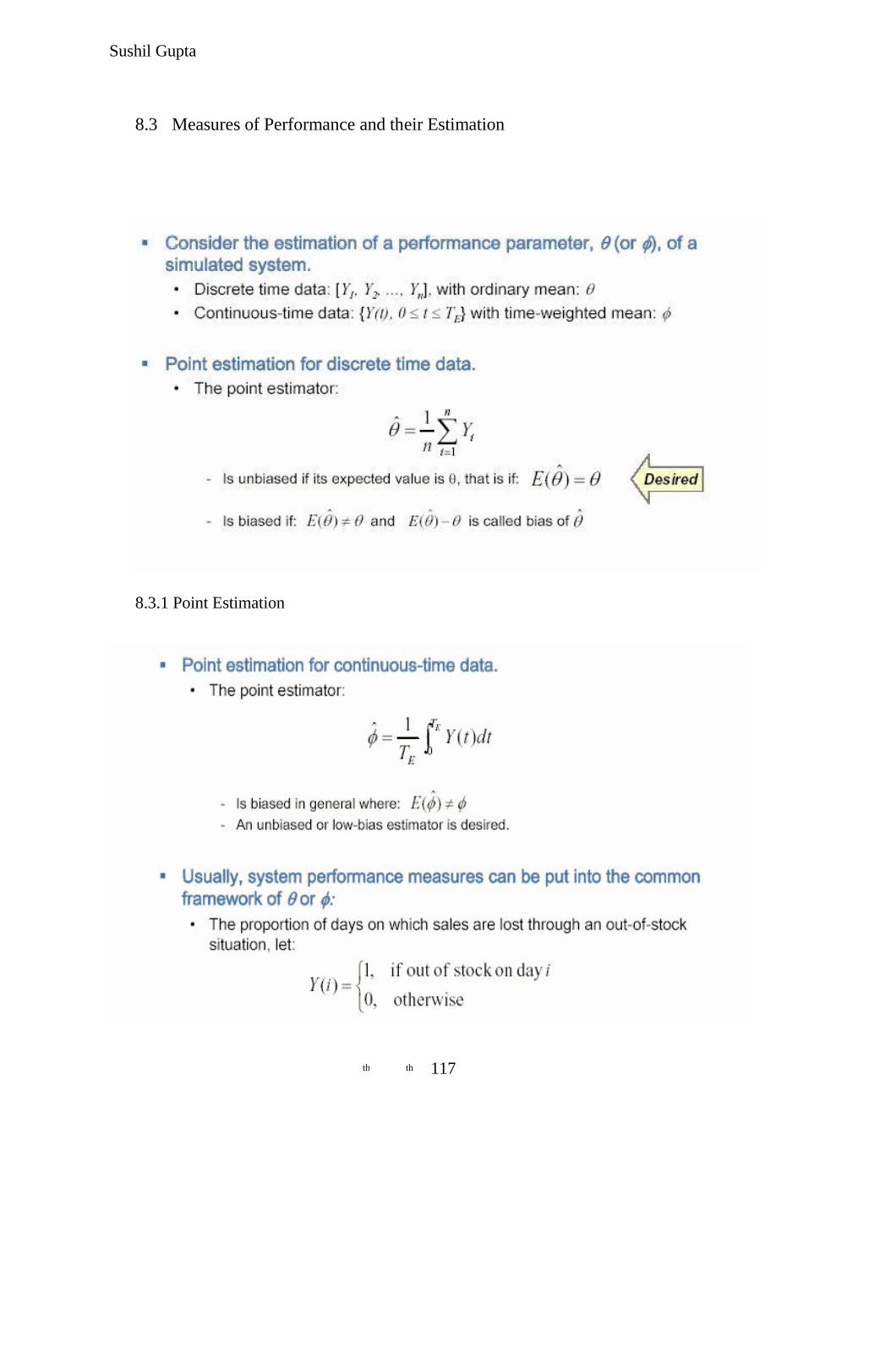
Sushil Gupta
8.3 Measures of Performance and their Estimation
8.3.1 Point Estimation
117 th th
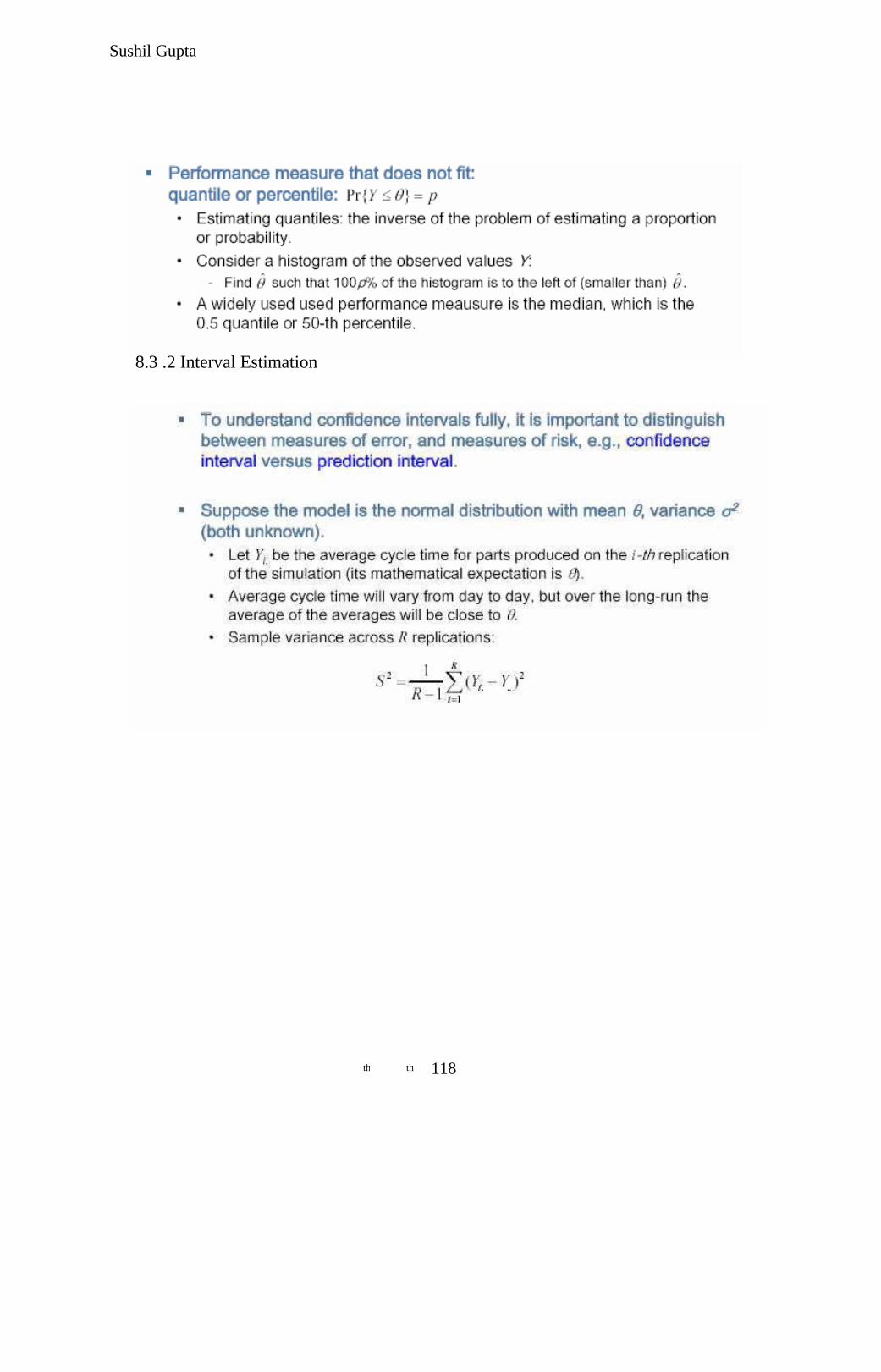
Sushil Gupta
8.3 .2 Interval Estimation
118 th th
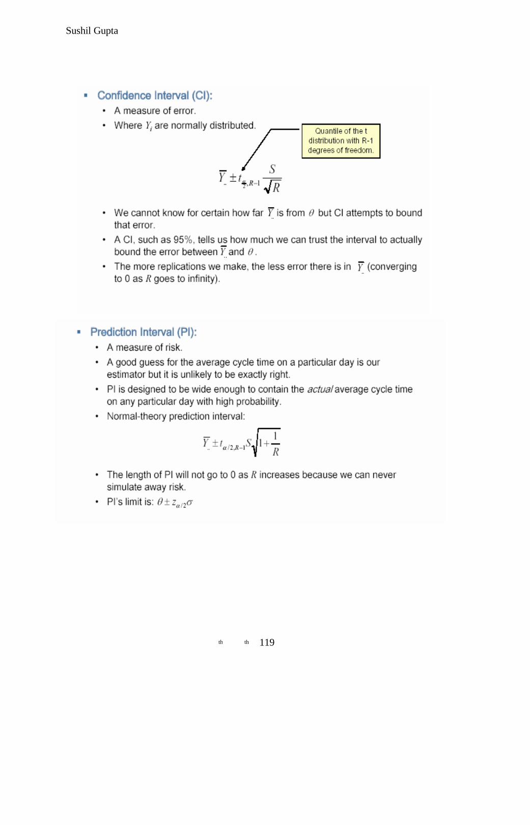
Sushil Gupta
119 th th
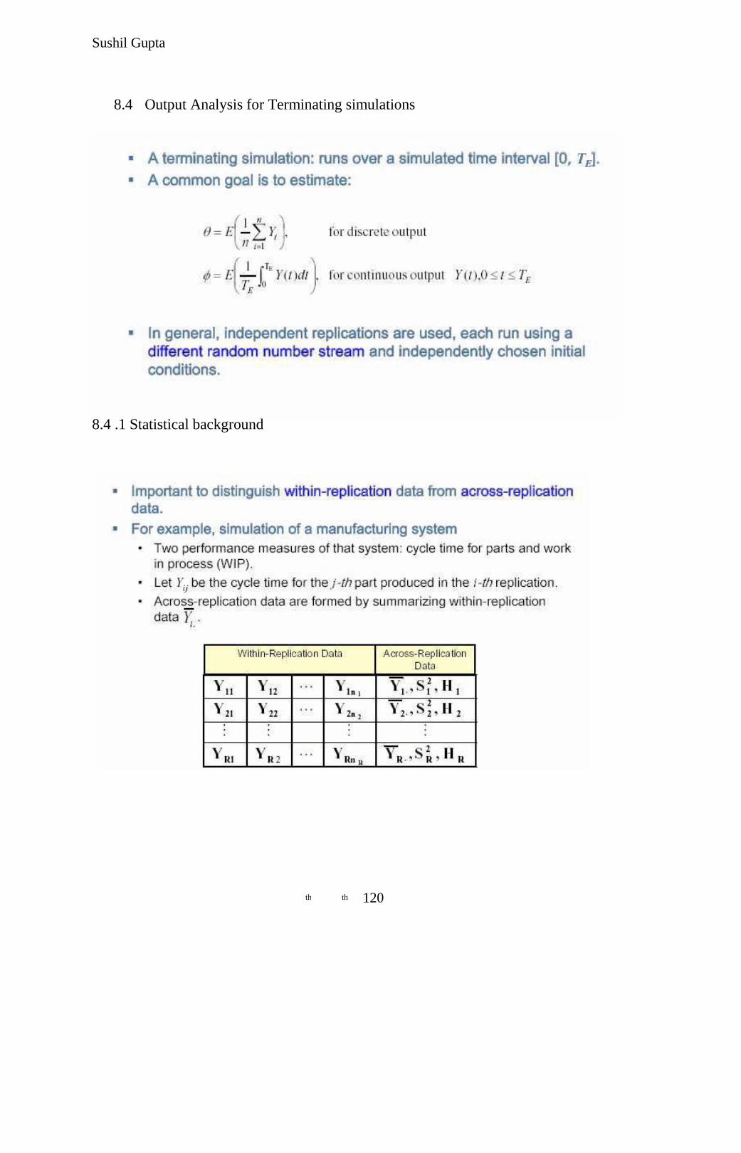
Sushil Gupta
8.4 Output Analysis for Terminating simulations
8.4 .1 Statistical background
120 th th
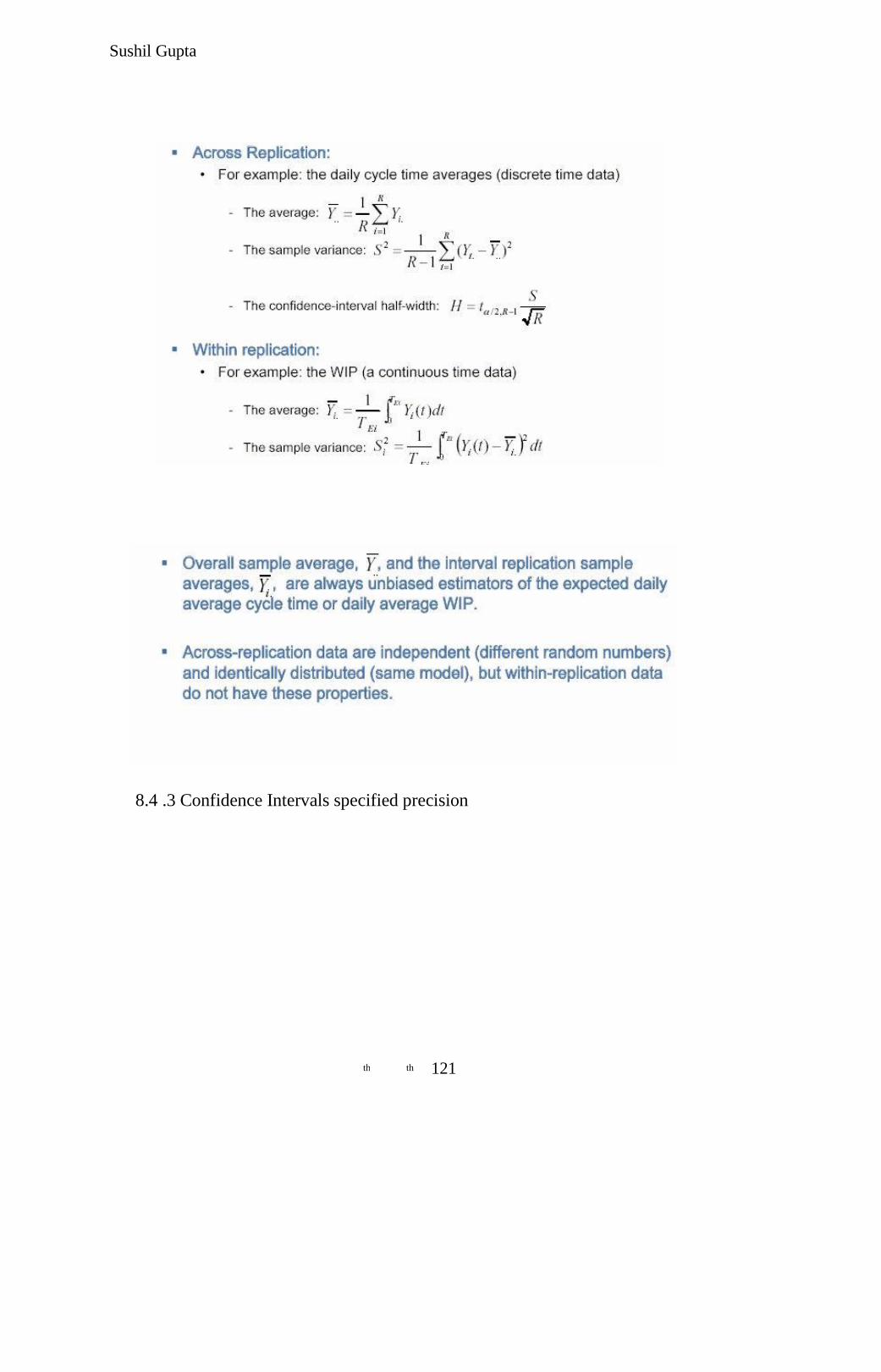
Sushil Gupta
8.4 .3 Confidence Intervals specified precision
121 th th
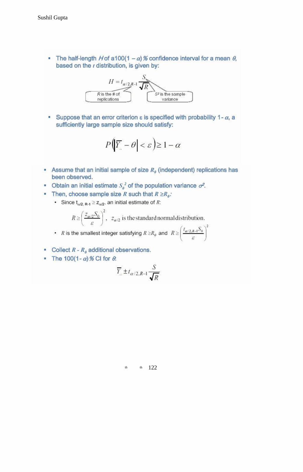
Sushil Gupta
122 th th

Sushil Gupta
8.4 .4 Confidence Intervals for Quantiles
123 th th
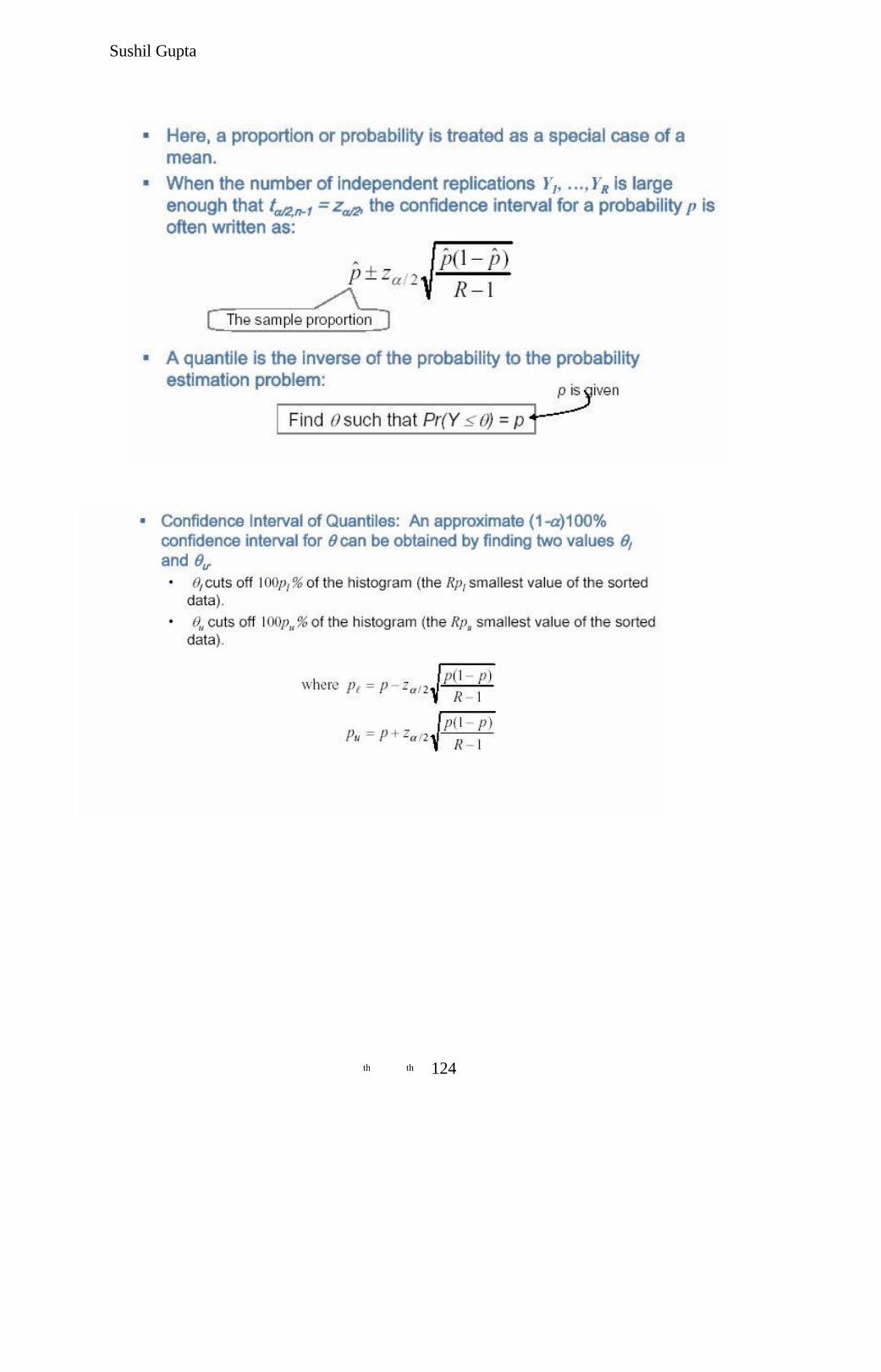
Sushil Gupta
124 th th
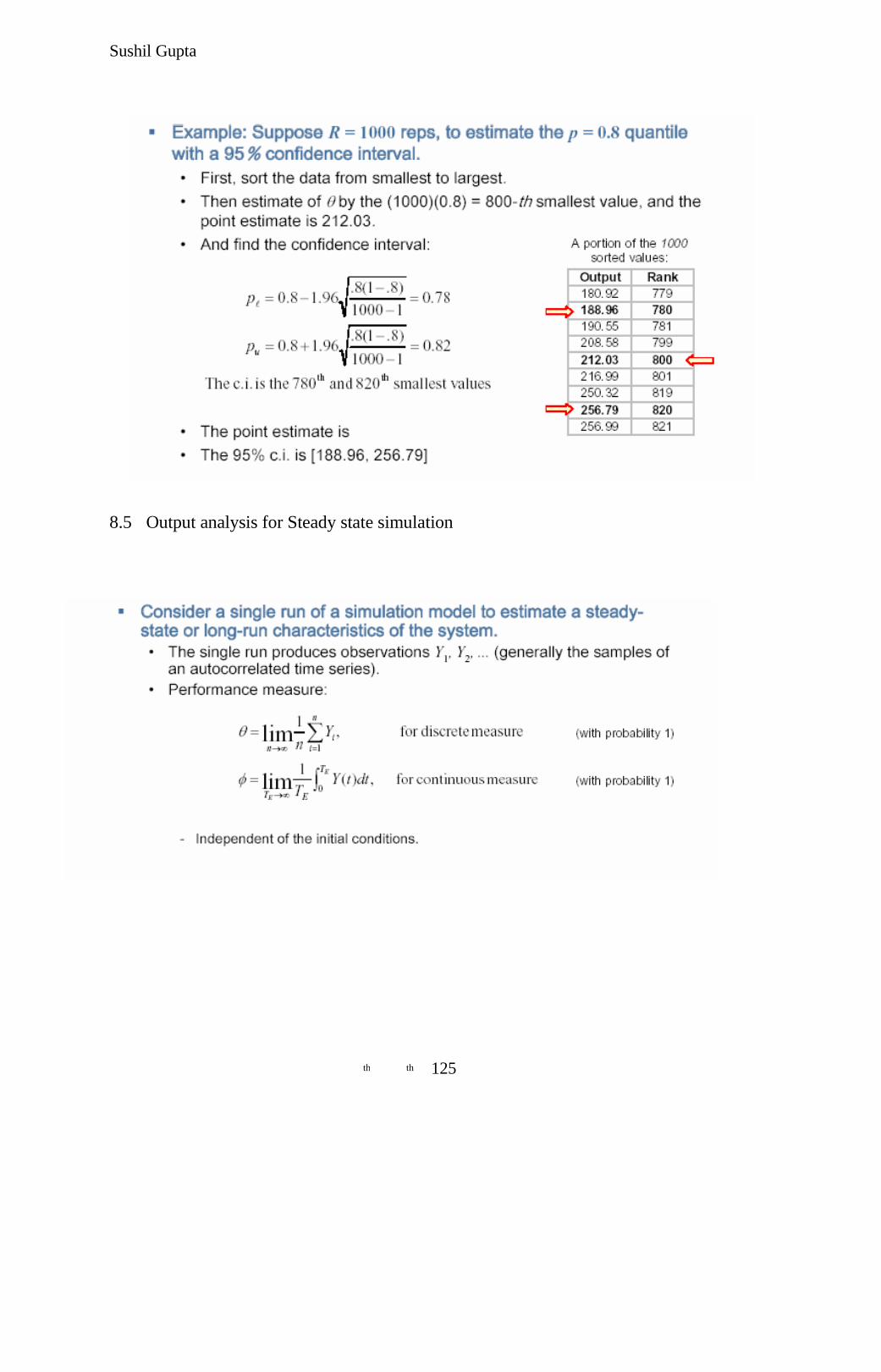
Sushil Gupta
8.5 Output analysis for Steady state simulation
125 th th
Sushil Gupta
8.5 .1 Initialization Bias
126 th th
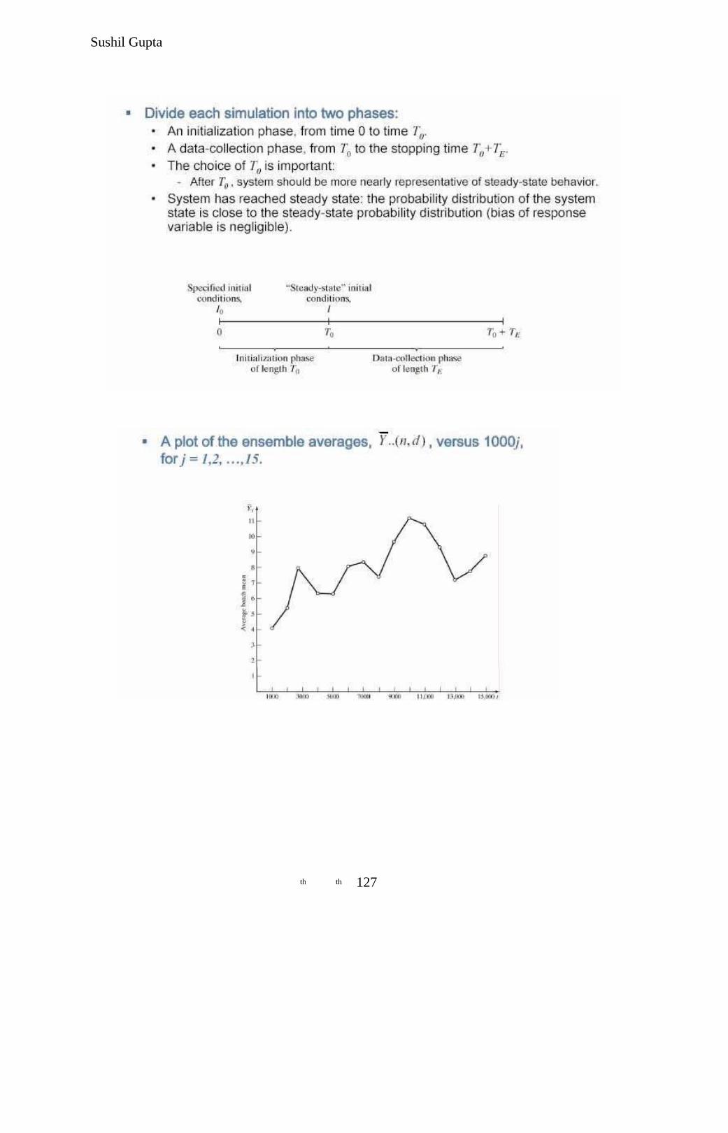
Sushil Gupta
127 th th
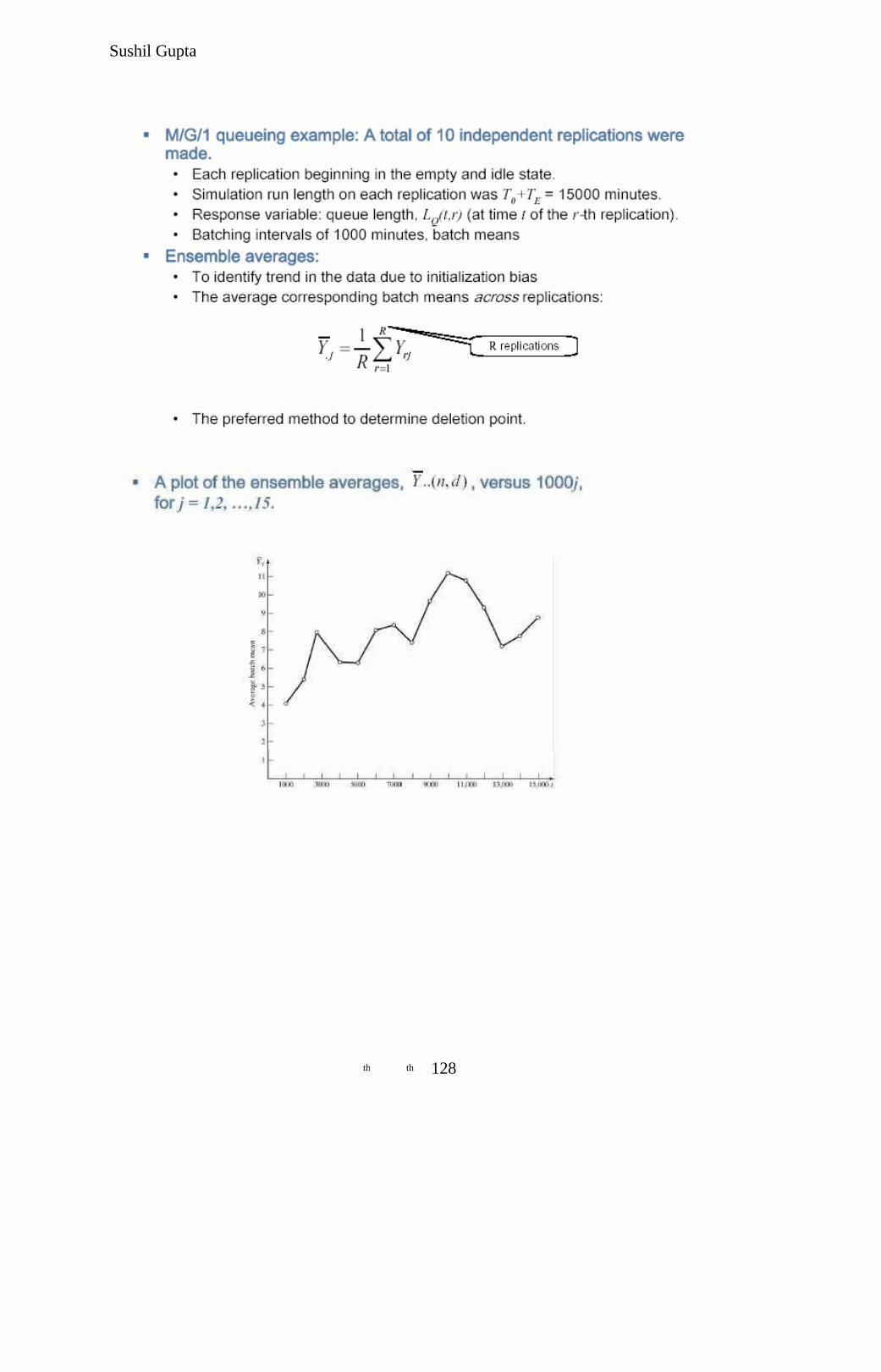
Sushil Gupta
128 th th
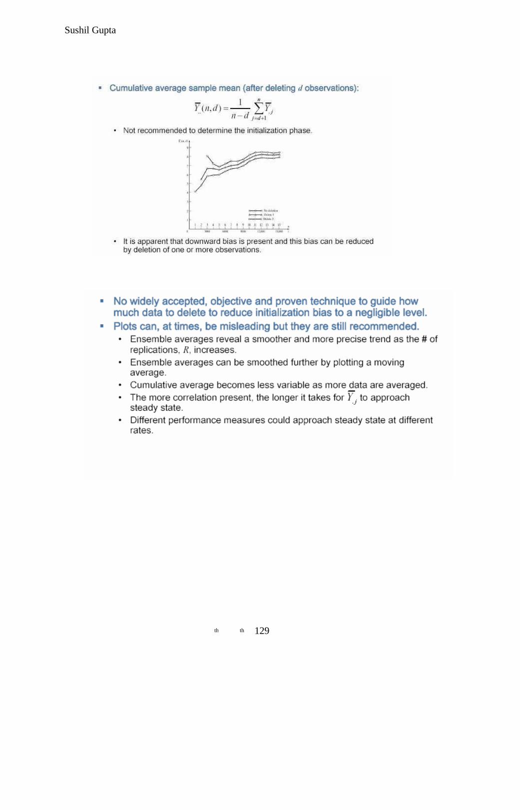
Sushil Gupta
129 th th
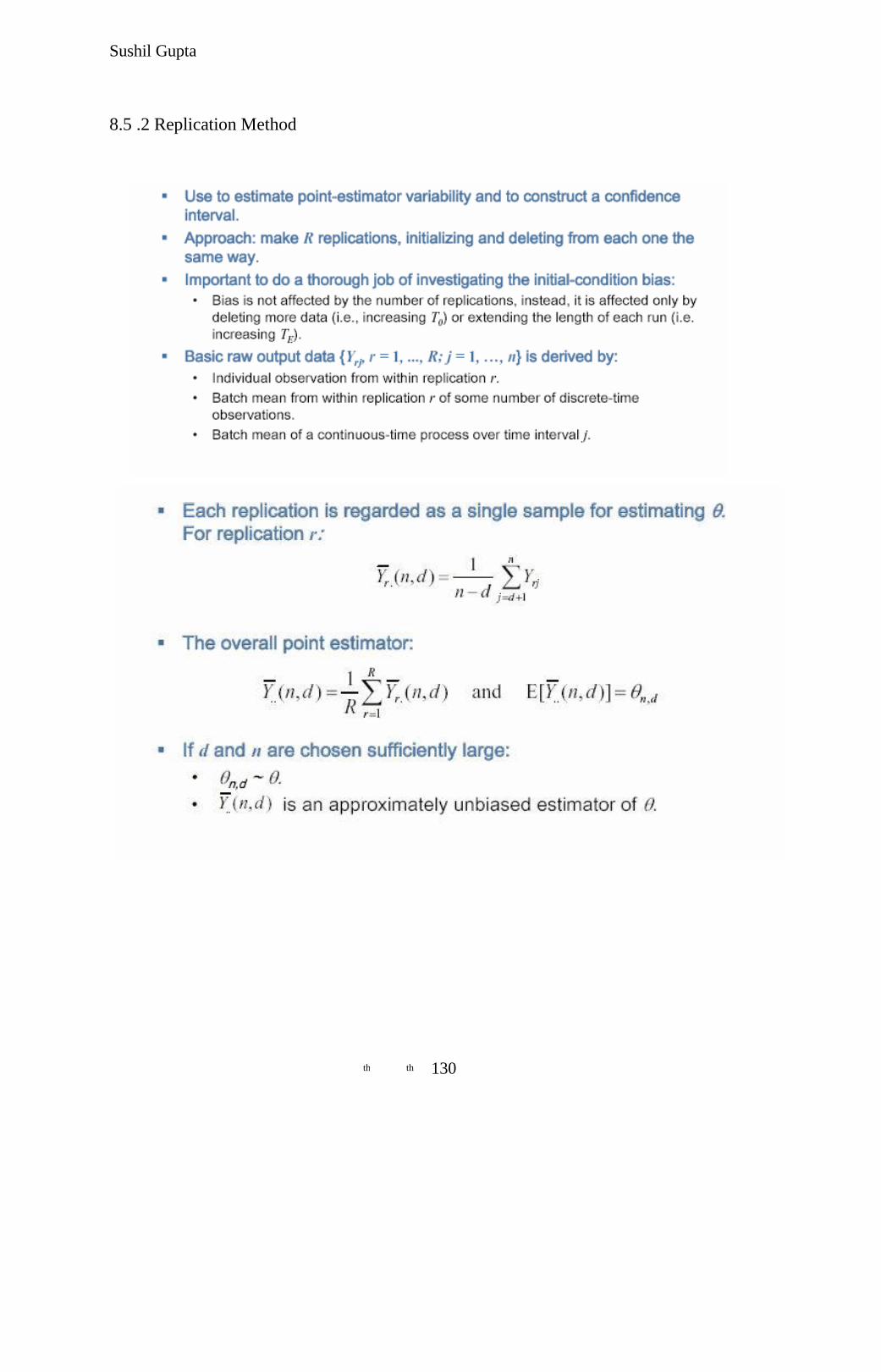
Sushil Gupta
8.5 .2 Replication Method
130 th th
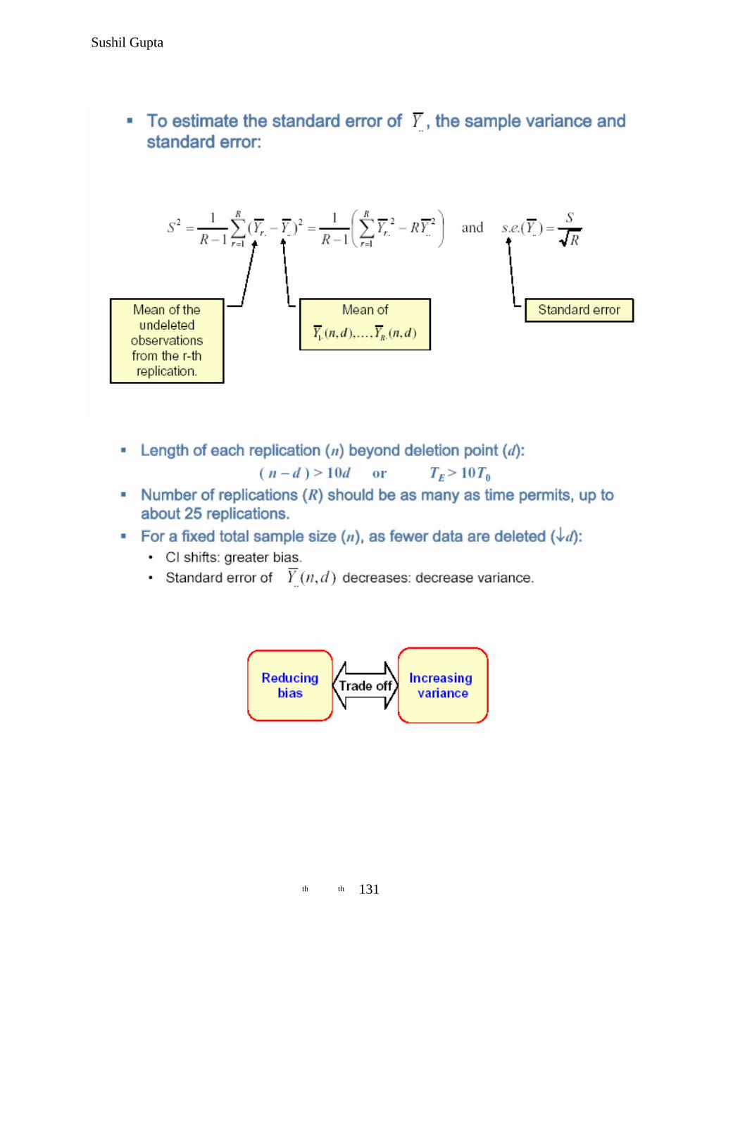
Sushil Gupta
131 th th
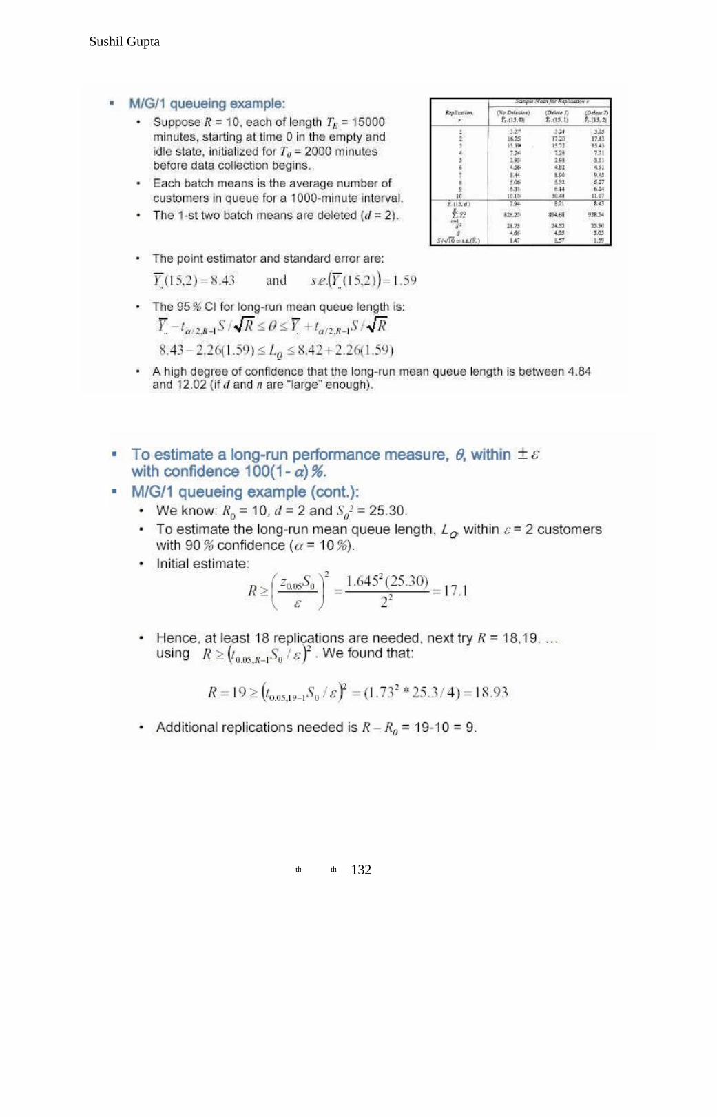
Sushil Gupta
132 th th
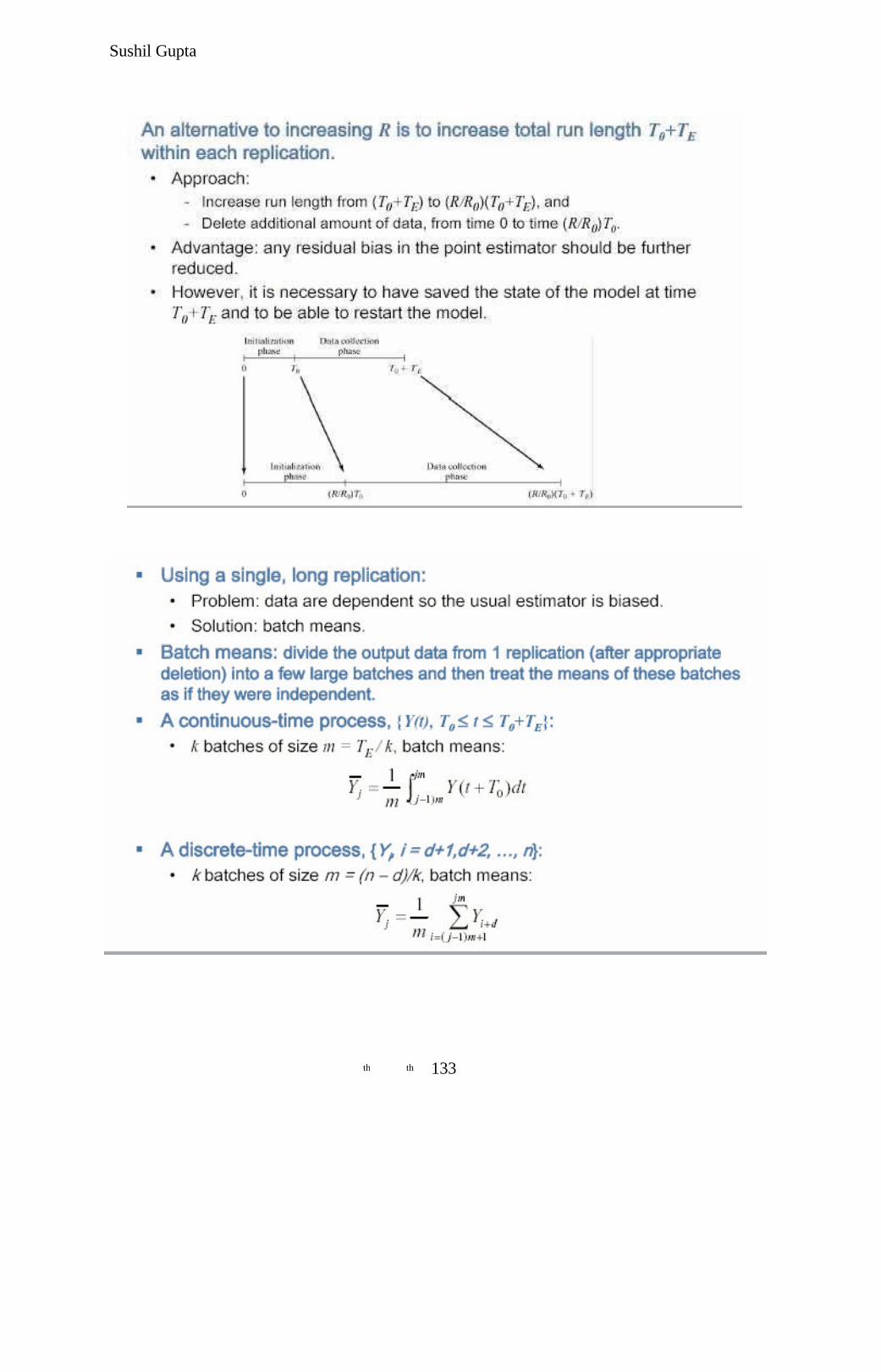
Sushil Gupta
133 th th
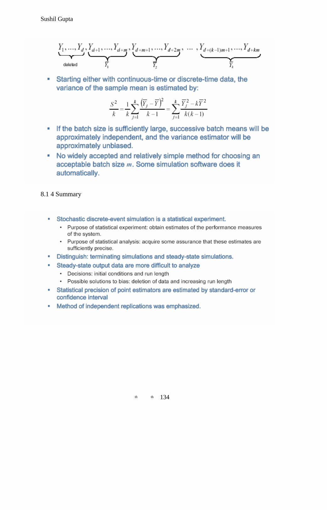
Sushil Gupta
8.1 4 Summary
134 th th
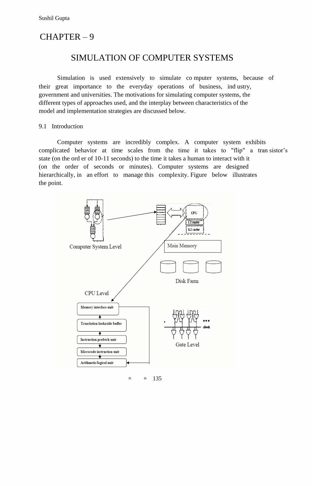
Sushil Gupta
CHAPTER – 9
SIMULATION OF COMPUTER SYSTEMS
Simulation is used extensively to simulate co mputer systems, because of
their great importance to the everyday operations of business, ind ustry,
government and universities. The motivations for simulating computer systems, the
different types of approaches used, and the interplay between characteristics of the
model and implementation strategies are discussed below.
9.1 Introduction
Computer systems are incredibly complex. A computer system exhibits
complicated behavior at time scales from the time it takes to "flip" a tran sistor‘s
state (on the ord er of 10-11 seconds) to the time it takes a human to interact with it
(on the order of seconds or minutes). Computer systems are designed
hierarchically, in an effort to manage this complexity. Figure below illustrates
the point.
135 th th
Sushil Gupta
Different levels of abstraction
• At a high level of abstraction (the system level) one might view computational activity in terms of tasks circulating among servers, queueing for service when a
server is busy.
• A lower level in the hierarchy can view the activity among components of a
given processor (its registers, its memory hierarchy).
• A lower level still one views the activity of functional units that together make
up a central processing unit.
• At an even lower level one can view the logical circuitry that makes it all
happen.
Simulation is used extensively at every level of this hierarchy, with result s from one
level being used at another. For instance, engineers working on designing a new chip will begin
by partitioning the chip functionally, establish interfaces between the subsystems, then design
and test the subsystems individually. Given a subsystem design, the electrical properties of the
circuit are first studied, using a circuit simulator that solves differential equations describing
electrical behavior. At this level engineers work to ensure that signal timing is correct throughout
the circuit, and that the electrical properties fall within the parameters intended by the design.
Once this level of validation has been achieved, the electrical behavior is abstracted into logical
behavior; e.g., signals former ly thought of as thought of as logical 1's or 0's. A different type of
simulator is next used to test the correctness of the circuit's logical behavior. A common testing
technique is to present the design with many different sets of logical inputs for which the desired
logical outputs are known. Discrete-event simulation is used to evaluate the logical response of
the circuit to each test vector, and is also used to evaluate timing. Once a chip‘s subsystems are
designed and tested, the designs are integrated, and then the whole system is subjected to testing,
again by simulation.
At a higher level one simulates using functional abstractions. For instance, a memory
chip could be modeled simply as an array of numbers and a reference to memory as just an
indexing operation. A special type of description language exists for this level, called ―register-
transfer language‖. This is like a programming language, with preassigned names for registers
and other hardware-specific entities, and with assignment statements used to indicate data
transfer between hardware entities. For example, the sequence below loads into register R3 the
data whose memory address is in register R6, subtracts one from it, and writes the result into the
memory location that is word-adjacent (a word in this example is 4 bytes in size) to the location
first read.
R3=M [R6]; R3=R3-1;
R6=R6+4; M [R6] =R3;
The abstraction makes sense when one is content to assume that the memory works, and
that the time to put a datum in or out is a known constant. The "known constant" is a value
resulting from analysis at a lower level of abstraction. Functional abstraction is also
136 th th

Sushil Gupta
commonly used to simulate subsystems of a central processing unit (CPU), when studying how
an executing program exercises special architectural features of the CPU.
At higher level still one might study how an input-output (I/O) system behave in response
to execution of a computer program. The program's behavior may be abstracted to the point of
being modeled but with some detailed description of I/O demands, e.g., with a Markov-chain
that with some specificity describes an I/O operation as the Markov chain transitions. The
behavior of the I/O devices may be abstracted to the point that all that is considered is how long
it takes to complete a specified I/O operation. Because of these abstractions one can simulate
larger systems, and simulate them more quickly. The execution of a program is modeled with a
randomly sampled CPU service interval; its I/O demand is modeled as a randomly sampled
service time on a randomly sampled I/O device.
9.2 Simulation Tools
Hand-in-hand with different abstraction levels one finds different tools used to perform and
evaluate simulations.
An important characteristic of a tool is how it supports model building. In many tools
one constructs networks of components whose local behavior is already known and already
programmed into the tool. This is a powerful paradigm for complex model construction. At the
low end of the abstraction hierarchy, electrical circuit simulators and gate-level simulators are
driven by network descriptions. Likewise, at the high end of the abstraction hierarchy, tools that
sirnulate queueing networks and Petri nets are driven by network descriptions, as are
sophisticated commercial communication-system simulators that have extensive libraries of
preprogrammed protocol behaviors.
VHDL Language
• A very significant player in computer-system design at lower levels of abstraction is the
VHDL language.
• VHDL is the result of a U.S. effort in the 1980s to standardize the languages used to
build electronic systems for the government.
• VHDL serves both as a design specification and as a simulation specification.
• VHDL is a rich language, full of constructs specific to digital systems, as well as the
normal constructs one finds in a procedural programming language.
• It achieves its dual role by imposing a clear separation between system topology and
system behavior.
• Design specification is a matter of topology, whereas simulation specification is a matter
of behavior.
• The language promotes user-defined programmed behavior.
• VHDL is also innovative in its use of abstract interfaces which different ''architectures‖ at
different levels of abstraction may be attached.
• VHDL is widely used in the electrical engineering community but is hardly used outside
of it.
137 th th
Sushil Gupta
Disadvantage of VHDL
• VHDL is a big language, requiring a substantive VHDL compiler, and vendors typically
target the commercial market at prices that exclude academic research.
Advantage of VHDL
• The relative rigidity of the programming model makes possible graphical model
building, thereby raising the whole model-building endeavor up to a higher level of
abstraction. Some tools have so much preprogrammed functionality that it is to design
and run a model without writing a single line of computer code.
9.2 .1 Process Orientation
• A process-oriented view implies that the tool must support separately schedulable "user
threads."
• A ―user thread" is a separately schedulable thread of execution control implemented as
part of a single executing process.
• A group of user threads operate in the same process memory space, with each thread
having allocated to it a relatively small portion of that space for its own use.
• The private space is used to store variables that are local to the thread, and information
needed to support the suspension and resumption of that thread.
• In process-oriented simulations, a thread is executed at a particular point in simulation
time, say t, as a result of some event being scheduled at time t; the thread execution is in
some sense the event handler.
• The thread yields by executing a statement whose semantics mean "suspend this thread
until the following condition occurs‖
• The hold statement is a classic example of this, it specifies how long in simulated time
the thread suspends.
• The CSIM model has examples of all of these.
Execution of CSIM Model
• The model is compiled and linked with CSIM libraries, creating an executable which,
when run, simulates the model.
• The main procedure associated with any C++ program—where program execution
begins—is buried inside the CSIM kernel.
• Beginning execution, control enters inside the CSIM kernel where initialization is done;
then the kernel calls procedure sim.
• CSIM requires a modeler to declare a procedure called sim, and that sim call create to
turn the call into a thread. This call creates the first thread.
• In the specific example of interest that thread generates customers, 1000 of them. It enters
a loop where it first suspends for an exponentially distributed period of time (an
interarrival delay), and after that delay simply creates a new customer, and returns to the
top of the loop. The call to customer creates a new thread.
138 th th

Sushil Gupta
• sim calls customer, which calls create. create allocates the internal data structures for the
new thread, schedules that new thread to execute at the current simulation time, but before executing the thread further, control is returned to sim.
• On receiving back control, sim immediately suspends through a hold call, and the
scheduler selects the thread whose invocation time is least among all executable threads.
• Almost always this will be the customer thread just created. This thread begins execution
at the call to use, which suspends the thread until all customers generated before it have
finished their executions, and then an implicit hold is performed on behalf of the thread,
modeling its service delay.
CSIM Example
Threads access variables that are globally visible to all threads, and variables that are
local to a specific thread. Variables Tot al Customers and NumberOf Customers are examples
of global variables; local variables i (in sim) and service (in customer) are examples of local
variables. Every instance of customer has its own copy of service. Local variables, the location
of where a thread resumes execution, and the contents of machine registers at the time a thread
suspended are all part of the thread state. To start a thread's execution, the scheduler must restore
all of a thread's state to the appropriate places. There are different ways to store and restore a
thread's state. The most common involve the program's runtime stack. When a program makes
a procedure call, the runtime system pushes a new "stack frame" onto the stack. A stack frame
contains the return address of the calling r outine, copies of input arguments to the procedure, and
space for local variables used by the called procedure. A machine register called the stack-frame
pointer contains the address of the first byte of the frame; machine code that references local
variables does so using addressing modes that specify an offset from the stack-frame pointer and
cause the hardware to compute the actual address by adding the offset to the contents of the
stack-frame pointer. When the called procedure returns control to the caller, the runtime system
pops its frame off the stack.
139 th th
Sushil Gupta
Fig. 9.2 Runtime stack in threaded simulation
Figure 9.2 illustrates a sequence of procedures and the stack of frames present on the first
call to hold. The call to hold suspends the thread, and when the thread executes once again it
will require all the information shown on the stack. Consequently the threading mechanism save
this portion of the stack, and restore it before the thread is executed again. CSIM's approach is to
have all threads use the same stack space as they execute, with the frame for the first procedure in the thread body always starting at the same memory location. When the thread
suspends, the CSIM kernel copies the used stack into separate storage associated with the thread.
To restore a thread, the CSIM kernel first copies the previously stored stack into the fixed stack
position, then lets the normal runtime control take over. The CSIM kernel also saves and
restores machine registers. An alternative approach to thread stack management avoids the
copying costs by preallocating memory for the stack of each different thread. Machine
registers must still be saved and restored, but a switch between threads is faster because only the
stack pointer must be changed, not the stack itself. The key limitation of such an approach is that
one must declare ahead of time the maximum stack size a thr ead may require, and there is
always the danger of the thread‘s pushing the stack beyond its allocation.
Process-oriented simulators are known to be slower than event-oriented simulators,
stack management being a key contributing factor. Depending on the threading implementation,
there may be additional factors. CSIM‘s threads are tailored to simulation, and the internal
scheduling mechanisms are purely temporal ones. However, threading is a concept that extends
well beyond simulation and threads exist in more general forms.
The problem for a simulator is that it wants to select the next thread to run, based on
simulation time. Most thread systems have ways of explicitly making a blocked thread runnable,
and of having a running thread block itself. The simulation scheduler can itself be a thread. When it runs, it identifies the next thread to run, as a function of an ordinary event-list, puts that
thread in the runnable set, and blocks itself. The one thread that can now be run does, and as a
part of its suspension sequence causes the scheduler to be runnable, and blocks itself.
9.2 .2 Event Orientation
• An event-oriented simulator is much simpler to design and implement using a general
programming language.
• The semantics of the program expressing a model are the semantics of the programming
language; there is no hidden activity akin to stack management or thread scheduling.
• It is natural to use object oriented techniques and express a simulation in terms of
messages passed between simulation objects.
• Languages like C++ and Java are outstanding for developing abstract base classes to
express the general structure of the simulator.
• In such an approach model building entails development of concrete classes derived from
the base classes, which includes expression of their methods.
140 th th

Sushil Gupta
Example
We suppose a simulation system has an abstract base class for all simulation objects, and
for all events comrnunicated below objects. Figure displays a simple example of such base
classes, in C++. The SimEvt class defines an interface for all event data structures a user would
define. The SimEvt base class contains a ―private‖ data member that stores the time-stamp of a
delivered event, and contains a ―public‖ method that allows any code to see what time-stamp is.
Class SimScheduler is declared to be a ―friend class‖ which means that its methods have the
same access privileges to an event‘s data as does the SimEvt class. The last bit of mystery is the
functions ~SimEvt and ~SimObj prefaced by the keyword virtual.
A modeler may tailor to the application, by definition, new event classes that include the
entire interface of the SimEvt class. PktEvt is an example of this. The user wished for the event
to carry a data packet of general length, and so endows the class with the infrastructure necessary
to store and access that packet. The user creates a ―derived‖ instance of the class by calling the
PktEvt constructor , which initializes its specialized data structures. The critical feature is that
pointer to an PktEvt instance can b passed to any routine with a type declaration of SimEvt, and
that routine can call the SimEvt methods and deal with the event in those terms.
This is exactly what happens when a simulation object schedules an event.
class SimEvt {
friend bool operator<(const SimEvt &el, const SimEvt &e2); friend bool
operator==(const SimEvt &el, const SimEvt &e2); friend class
SimScheduler;
private; stime _time;
public: SimEvt();
Virtual –SimEvt(); Void set-time (stime when) {_time =when ;}
stime get_timeQ {return _time ;}
};
class SimObj {
protected:
public: SimObj();
Virtual –SimObj(); Virtual void acceptEvt(SimEvt *)=0;
}; class SimScheduler{
public: SimScheduler();
Int ScheduleEvt(SimObj *, SimEvt *, stime delay); Stime now();
}; class PktEvt : public SimEvt {
private: int pkt_length;
void *packet; public:
PktEvt();
141 th th
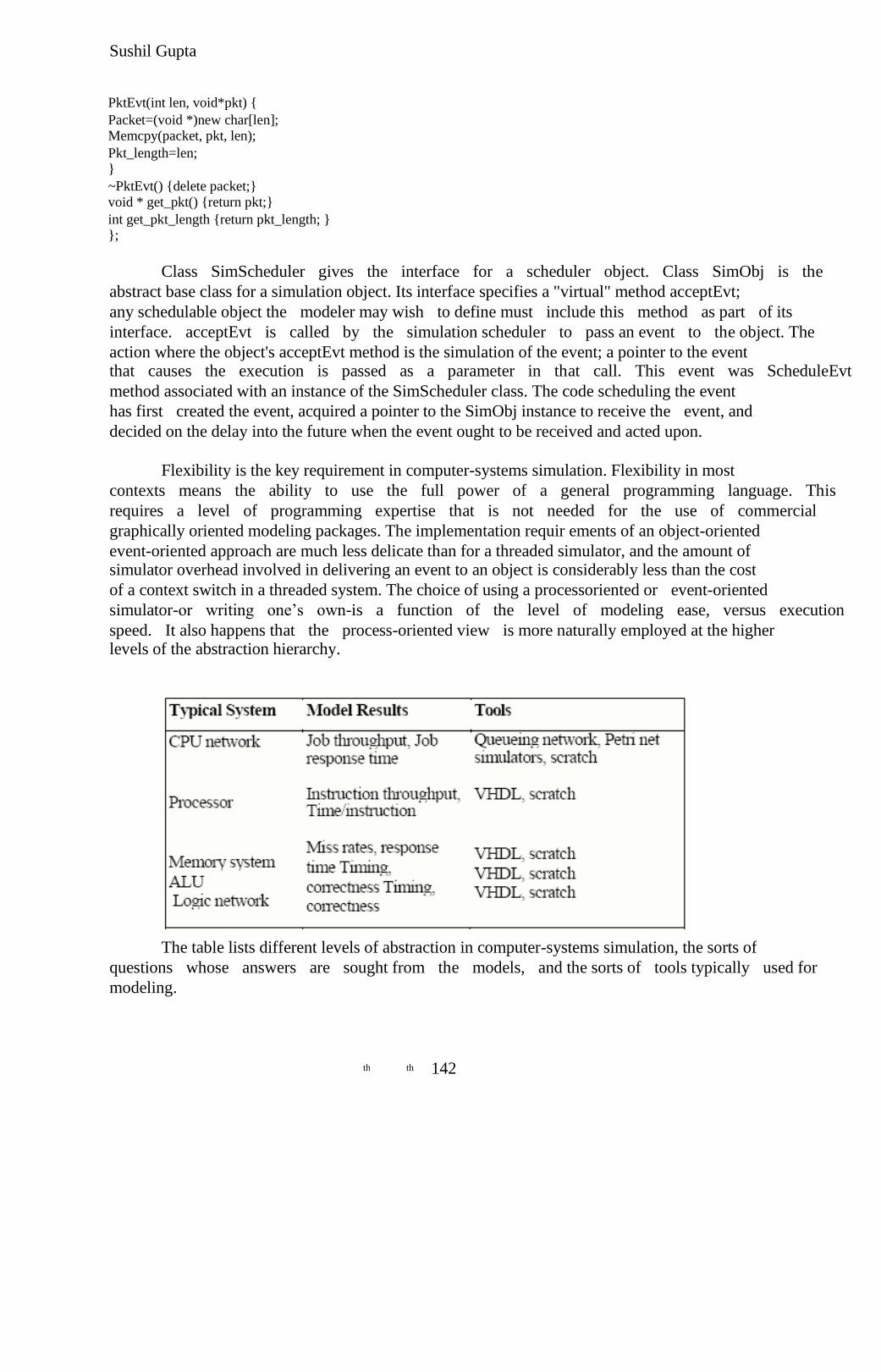
Sushil Gupta
PktEvt(int len, void*pkt) {
Packet=(void *)new char[len]; Memcpy(packet, pkt, len);
Pkt_length=len; }
~PktEvt() {delete packet;}
void * get_pkt() {return pkt;}
int get_pkt_length {return pkt_length; }
};
Class SimScheduler gives the interface for a scheduler object. Class SimObj is the
abstract base class for a simulation object. Its interface specifies a "virtual" method acceptEvt;
any schedulable object the modeler may wish to define must include this method as part of its
interface. acceptEvt is called by the simulation scheduler to pass an event to the object. The
action where the object's acceptEvt method is the simulation of the event; a pointer to the event that causes the execution is passed as a parameter in that call. This event was ScheduleEvt
method associated with an instance of the SimScheduler class. The code scheduling the event
has first created the event, acquired a pointer to the SimObj instance to receive the event, and
decided on the delay into the future when the event ought to be received and acted upon.
Flexibility is the key requirement in computer-systems simulation. Flexibility in most
contexts means the ability to use the full power of a general programming language. This
requires a level of programming expertise that is not needed for the use of commercial
graphically oriented modeling packages. The implementation requir ements of an object-oriented
event-oriented approach are much less delicate than for a threaded simulator, and the amount of
simulator overhead involved in delivering an event to an object is considerably less than the cost
of a context switch in a threaded system. The choice of using a processoriented or event-oriented
simulator-or writing one‘s own-is a function of the level of modeling ease, versus execution
speed. It also happens that the process-oriented view is more naturally employed at the higher
levels of the abstraction hierarchy.
The table lists different levels of abstraction in computer-systems simulation, the sorts of
questions whose answers are sought from the models, and the sorts of tools typically used for
modeling.
142 th th
Sushil Gupta
9.3 Model Input
There are different means of providing input to a model. The model might be driven by ·
Stochastically generated input, using either simple or complicated operational assumptions, used
at the high end of the abstraction. Useful for the study the system behavior over a range of
scenarios.
• Trace input, measured from actual systems used at lower levels.
• High-level systems simulations accept a stream of job descriptions; CPU simulations
accept a stream of instruction descriptions, memory simulations accept a stream of
memory references; and gate-level simulations accept a stream of logical signals.
• Computer systems modeled as queueing networks typically interpret "customers" as
computer programs; servers typically represent services such as attention by the CPU or
an input/output system.
• Random sampling generates customer interarrival times, and it may also be used to
govern routing and time-in-service.
• However, it is common in computer systems contexts to have routing and service times
be state dependent; e.g., the next server visited is already specified in the customer's
description, or may be the attached server with least queue length.
9.3 .1 Modulated Poisson Process
• An input model that is sometimes used to retain a level of tractability is a modulated
Poisson process, or MPP.
• The underlying framework is a continuous-time Markov chain (CTMC).
• A CTMC is always in some state; for descriptive purposes states are named by the
integers: 1, 2,....
• The CTMC remains in a state for a random period of time, transitions randomly to
another state, stays there for a random period of time, transitions again, and so on.
• The CTMC behavior is completely determined by its generator matrix, Q = {q,j}. For
states i<> j, entry q,j describes the rate at which the chain transitions from state i into
state j.
• The rate describes how quickly the transition is made; its units are transitions per unit
simulation time.
• Diagonal element q,i is the negated sum of all rates out of state i : q,i = - € qi,j
• An operational view of the CTMC is that upon entering a state i , it remains in that state
for an exponentially distributed period of time, the exponential having rate –qi,i Making
the transition, it chooses state j with probability –qi,j / qi,i .
• Many CTMCs ar e ergodic, meaning that, left to run forever, every state is visited
infinitely often.
143 th th
Sushil Gupta
• In an ergodic chain I, denotes state i‘s stationary probability, which we can interpret as
the long-term average fraction of time the CTMC is in state i.
• A critical relationship exists between stationary probabilities and transition rates: for
every state i,
q = j qj,i i i,j
9.3 .2 Virtual Memory Referencing
• Randomness can also be used to drive models in the middle levels of abstraction.
• In such a system, the data and instructions used by the program are organized in units
called pages.
• All pages are the same size, typically 210 to 212 bytes in size.
• The physical memory of a computer is divided into page frames, each capable of holding
exactly one page.
• The decision of which page to map to which frame is made by the operating system.
• As the program executes, it makes memory references to the "virtual memory," as though
it occupied a very large memory starting at address 0, and is the only occupant of the
memory.
• On every memory reference made by the program, the hardware looks up the identity of
the page frame containing the reference, and translates the virtual address into a physical
address.
• The hardware may discover that the referenced page is not present in the main memory; this is called & page fault
• When a page fault occurs, the hardware alerts the operating system, which then takes
over to bring in the referenced page from a disk and decides which page frame should
contain it.
• The operating system may need to evict a page from a page frame to make room for the
new one.
• The policy the operating system uses to decide which page to evict is called the
"replacement policy‖.
• The quality of a replacement policy is often measured in ter ms of the fraction of
references made whose page frames are found immediately, the hit ratio.
• Virtual memory systems are used in computers that support concurrent execution of
multiple programs.
• In order to study different replacement policies one could simulate the memory-
referencing behavior of several different programs, simulate the replacement policy, and
count the number of references that page-fault.
• Virtual memory works well precisely because programs do tend to exhibit a certain type
of behavior, so-called locality of reference.
• The program references tend to cluster in time and space, that when a reference to a new
page is made and the page is brought in from the disk, it is likely that the other data or
instructions on the page will also soon be referenced.
• In this way the overhead of bringing in the page is amortized over all the references made
to that page before it is eventually evicted.
144 th th
Sushil Gupta
• A program's referencing behavior can usually be separated into a sequence of "phases,"
where during each phase the program makes references to a relatively small collection of
pages called its working set.
• Phase transitions essentially change the program's working set. The challenge for the
operating system is to recognize when the pages used by a program are no longer in its
working set, for these are the pages it can safely evict to make room for pages that are in
some program's working set.
9.4 High-Level Computer System Simulation
Here we illustrate concepts typical of high-level computer simulations, by sketching a
simulation model of a computer system that services requests from the World Wide Web.
EXAMPLE
• A company that provides a major web site for searching and links to sites for Travel,
commerce, entertainment, and the like wishes to conduct a capacity planning study.
• The overall architecture of their system is shown in Figure.
• At the back end one finds data servers responsible for all aspects of handling specific
queries and updating databases.
• Data servers receive requests for service from application servers— machines dedicated
to running specific applications supported by the site.
• In front of applications are web servers that manage the interaction of applications with
the World Wide Web, and the portal to the whole system is a load-balancing router that
distributes requests directed to the web site among web servers.
• The goal of the study is to determine the site's ability to handle load at peak periods.
• The desired output is an empirical distribution of the access response time.
• Thus, the high-level simulation model should focus on the impact of timing at each level
that is used, system factors that affect that timing, and the effects of timing on contention
for resources.
145 th th
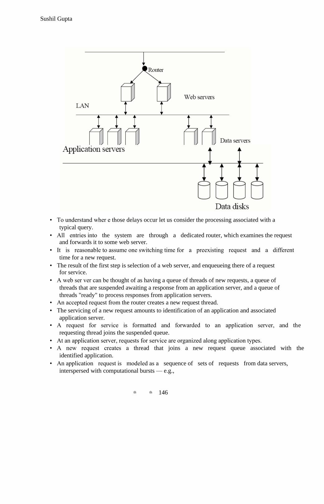
Sushil Gupta
• To understand wher e those delays occur let us consider the processing associated with a
typical query.
• All entries into the system are through a dedicated router, which examines the request and forwards it to some web server.
• It is reasonable to assume one switching time for a preexisting request and a different
time for a new request.
• The result of the first step is selection of a web server, and enqueueing there of a request for service.
• A web ser ver can be thought of as having a queue of threads of new requests, a queue of
threads that are suspended awaiting a response from an application server, and a queue of
threads "ready" to process responses from application servers.
• An accepted request from the router creates a new request thread.
• The servicing of a new request amounts to identification of an application and associated
application server.
• A request for service is formatted and forwarded to an application server, and the
requesting thread joins the suspended queue.
• At an application server, requests for service are organized along application types.
• A new request creates a thread that joins a new request queue associated with the
identified application.
• An application request is modeled as a sequence of sets of requests from data servers,
interspersed with computational bursts — e.g.,
146 th th
Sushil Gupta
burst 1
request data from Dl, D3 and D5
burst 2
request data from Dl and D2
burst 3
• An application server will implement a scheduling policy over sets of ready application
threads.
• A data server creates a new thread to respond to a data request and places it in a queue of
ready threads.
• A data server may implement memory-management policies, and may require further
coordination with the application server to know when to release used memory.
• Upon r eceiving service the thread requests data from a disk, and suspends until the disk
operation completes, at which point the thread is moved from the suspended list to the
ready list, and when executed again reports back to the application server associated with
the request.
• The thread suspended at the application server responds; eventually the application thread
finishes and reports its completion back to the web-server thread that initiated it, which in
turn communicates the results back over the Internet.
The web- site model is an excellent candidate for a threaded (process-oriented) appr oach
to modeling. There are two natural approaches for defining a process. One emulates our CSIM
example, defining each request as a process. The model would be expressed from the point of
view of a request going through the router, to a web server, and so on.
Disadvantage of query centered modeling
One complication with equating a query with a process is that it is not an exact fit to what happens in this model. A query passed from application server to data server may actually cause
multiple concur rent requests to the data disks—it is insufficient to "push" a query process from
router to disks and back. A query process can spawn concurrent supporting processes, which
implies encoding a fork-and-join synchronization mechanism (a process spawns new processes,
and waits for them to return). The CSIM example illustrated this by having the main thread
suspend, once all job arrival processes had been generated, until the last one finished.
Advantage of query centered modeling
The advantage to a query-centered modeling approach is clarity of expression, and the
ease with which query-or iented statistics can be gathered. A given query process can simply
measure its delays at every step along the way, and upon departing the system include its
observations in the statistical record the simulation maintains for the system.
147 th th
Sushil Gupta
An alternative process-oriented approach is to associate processes with servers. The
simulation model is expressed from an abstracted point of view of the servers' operating system.
Individual queries become messages that are passed between server pr ocesses. An advantage of
this approach is that it explicitly exposes the scheduling of query processing at the user level.
The modeler has both the opportunity and the responsibility to provide the logic of scheduling
actions that model processing done on behalf of a query. It is a modeling viewpoint that
simplifies analysis of server behavior — an overloaded server is easily identified by the length of
its queue of runnable queries. However, it is a modeling viewpoint that is a bit lower in
abstraction than the first one, and requires more modeling and coding on the part of the user.
An event-oriented model of this system need not look a great deal different than the
second of our process-oriented models. Queries passed as messages between servers have an
obvious event-oriented expression. A modeler would have to add to the logic, events, and event
handlers that describe the way a CPU passes through simulation time. In an event-oriented model
one would need to define events that reflect "starting" and "stopping" the processing of a query,
with some scheduling logic interspersed. Additional events and handlers need to be defined for
any "signaling" that might be done between servers in a process-oriented model. A process-
oriented approach, even one focused on servers rather than queries, lifts model expression to a
higher level of abstraction and reduces the amount of code that must be written. In a system as
complex as the web site, one must factor complexity of expression into the over all model-
development process.
9.5 CPU Simulation
The main challenge to making effective use of a CPU is to avoid stalling it, which
happens whenever the CPU commits to executing an instruction whose inputs are not all present.
A leading cause of stalls is the latency delay between CPU and main memory, which can be tens
of CPU cycles. One instruction may initiate a read,
e.g.,
load $2, 4($3)
which is an assembly-language statement that instructs the CPU to use the data in register 3
(after adding value 4 to it) as a memory address, and to put the data found at that address in
register 2. If the CPU insisted on waiting for that data to appear in register 2 before further
execution, the instruction could stall the CPU for a long time if the referenced address was not found in the cache. High-performance CPUs avoid this by recognizing that additional
instructions can be executed, up to the point where the CPU attempts to execute an instruction
that reads the contents of register 2,
e.g.,
add $4, $2, $5
148 th th
Sushil Gupta
This instruction adds the contents of registers 2 and 5 and places the result in register 4. If the
data expected in register 2 is not yet present, the CPU will stall.
To allow the CPU to continue past a memory load it is necessary to
• mark the target register as being unready
• allow the memory system to asynchronously load the target register while the CPU
continues on in the instruction stream
• stall the CPU if it attempts to read a register marked as unready
• Clear the unready status when the memory operation completes.
The sort of arrangement described above was first used in the earliest supercomputers,
designed in the 1960s. Modern microprocessors add some additional capabilities to exploit
instruction-level parallelism (ILP).
Pipelining
• The technique of pipelining has long been recognized as a way of accelerating the
execution of computer instructions.
• Pipelining exploits the fact that each instruction goes sequentially through several stages
in the course of being processed; separate hardware resour ces are dedicated to each stage,
permitting multiple instructions to be in various stages of processing concurrently
• A typical sequence of stages in an ILP CPU are as follows:
Instruction fetch : the instruction is fetched from the memory.
Instruction decode : the memory word holding the instruction is interpreted to
determine what operation is specified; the registers involved are identified.
Instruction issue : an instruction is "issued" when there are no constraints
holding it back from being executed. Constraints that keep an instruction from
being issued include data not yet being ready in an input register, and
unavailability of a functional unit (e.g., arithmetic-logicalunit) needed to execute
the instruction.
Instruction execute : the instruction is performed.
Instruction complete : results of the instruction are stored in the destination
register.
Instruction graduate : executed instructions are graduated in the order that they
appear in the order that they appear in the instruction stream.
9.6 Memory Simulation
149 th th
Sushil Gupta
• One of the great challenges of computer architecture is finding ways to effectively deal
with the increasing gap in operation speed between CPUs and main memory.
• The main technique that has evolved is to build hierarchies of memories.
• A relatively small memory—the L1 cache—operates at CPU speed. A larger memory—
the L2 cache— is larger, and operates more slowly.
• The main memory is larger still, and slower still. The smaller memories hold data that was referenced recently.
• Data moves up the hierarchy on demand, and ages out as it becomes disused, to make
room for the data in current use.
• For instance, when the CPU wishes to read memory location 100000, hardware will look
for it in the L1 cache, and failing to find it there, look for it in the L2 cache.
• If found there, an entire block containing that reference is moved from the L2 cache into
the L1 cache.
• If not found in the L2 cache, a block of data containing location 10000 is copied from the
main memory to the L2 cache, and part of that block is copied into the LI cache.
• It may take 50 cycles or more to accomplish this.
• After this cost has been suffered, the hope and expectation is that the CPU will continue
to make r eferences to data in the block brought in, because accesses to LI data are made
at CPU speeds.
• After a block ceases to be referenced for a time, it is ejected from the LI cache.
• It may remain in the L2 cache for a while, and be brought back into the LI cache if any
element of the block is referenced again.
• Eventually a block remains unreferenced long enough so that it is ejected also from the
L2 cache.
An alternative method copies back a block from one memory level to the lower level, at the
point the block is being ejected from the faster level. The write-through strategy avoids writing
back blocks when they are ejected, whereas the write-back strategy requires that an entire block
be written back when ejected, even if only one word of the block was modified, once.
The principal measure of the quality of a memory hierarchy is its hit ratio at each level. As
with CPU models, to evaluate a memory hierarchy design one must study the design in response
to a very long string of memory references. Direct-execution simulation can provide such
reference stream, as can long tr aces measured reference traffic. Nearly every caching system is a
demand system, which means that a new block is not brought into a cache before a reference is
made to a word in that block.
Set Associativity
• The concept of set associativity arises in response to the cost of the mechanism used to
look for a match.
• Imagine we have an L2 cache with 2 million memory wor ds.
• The CPU references location 10000—the main memory has, say, 212 words, so the L2
cache holds but a minute fraction of the main memory.
150 th th
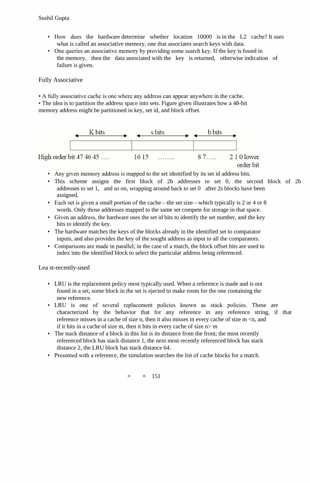
Sushil Gupta
• How does the hardware determine whether location 10000 is in the L2 cache? It uses
what is called an associative memory, one that associates search keys with data.
• One queries an associative memory by providing some search key. If the key is found in
the memory, then the data associated with the key is returned, otherwise indication of
failure is given.
Fully Associative
• A fully associative cache is one where any address can appear anywhere in the cache.
• The idea is to partition the address space into sets. Figure given illustrates how a 48-bit
memory address might be partitioned in key, set id, and block offset.
• Any given memory address is mapped to the set identified by its set id address bits.
• This scheme assigns the first block of 2b addresses to set 0, the second block of 2b
addresses to set 1, and so on, wrapping around back to set 0 after 2s blocks have been
assigned.
• Each set is given a small portion of the cache—the set size—which typically is 2 or 4 or 8
words. Only those addresses mapped to the same set compete for storage in that space.
• Given an address, the hardware uses the set id bits to identify the set number, and the key
bits to identify the key.
• The hardware matches the keys of the blocks already in the identified set to comparator
inputs, and also provides the key of the sought address as input to all the comparators.
• Comparisons are made in parallel; in the case of a match, the block offset bits are used to
index into the identified block to select the particular address being referenced.
Lea st-recently-used
• LRU is the replacement policy most typically used. When a reference is made and is not
found in a set, some block in the set is ejected to make room for the one containing the
new reference.
• LRU is one of several replacement policies known as stack policies. These are
characterized by the behavior that for any reference in any reference string, if that
reference misses in a cache of size n, then it also misses in every cache of size m <n, and
if it hits in a cache of size m, then it hits in every cache of size n> m
• The stack distance of a block in this list is its distance from the front; the most recently
referenced block has stack distance 1, the next most recently referenced block has stack
distance 2, the LRU block has stack distance 64.
• Presented with a reference, the simulation searches the list of cache blocks for a match.
151 th th

Sushil Gupta
• If no match is found, then by the stack property no match will be found in any cache of a
size smaller than 64, on this reference, for this reference string. If a match is found and
the block has stack distance k, then no match will be found in any cache smaller than size
k, and a match will always be found in a cache of size larger than k.
• Rather than record a hit or miss, one increment the kth element of a 64-element ar ray that
records the number of matches at each LRU level.
• To determine how many hits occured in a cache of size n, one sums up the counts of the
first n elements of the array.
• Thus, with a little arithmetic at the end of the run, one can determine (for each set cache)
the number of hits for every set of every size between 1 and 64.
Figure illustrates the evolution of an LRU list in response to a reference string.
• Under each reference is the state of the LRU stack after the reference is pr ocessed.
• The horizontal direction from left to right symbolizes the trace, reading from left to right.
• A hit is illustrated by a circle, with an arrow showing the migration of the symbol to the
top of the heap.
• The "hits" array counts the number of hits found at each stack distance.
• Thus we see that a cache of size 1 will have a hit ratio of 0/15, a cache of size 1 will have
a hit ratio of 1/15, and a cache of size 3 will have a hit ratio of 6/15.
• In one pass one can get hit ratios for varying set sizes, but it is important to note that each
change in set size corresponds to a change in the overall size of the entire cache
152 th th