System-level Analysis of Chilled Water SystemsAboard Naval Ships

Hessam Babaee, Julie Chalfant,Chryssostomos Chryssostomidis

MIT Sea GrantMassachusetts Institute of Technology

Cambridge, MAEmail: babaee@mit.edu

Amiel B. Sanfiorenzo †Puget Sound Naval Shipyard

and Intermediate Maintenance FacilityBremerton, WA

Abstract—A thermal management simulation tool isrequired to rapidly and accurately evaluate and miti-gate the adverse effects of increased heat loads in theinitial stages of design in all-electric ships. By reducingthe dimension of Navier-Stokes and energy equations,we have developed one-dimensional partial differen-tial equation models that simulate time-dependent hy-drodynamics and heat transport in a piping networksystem. Besides the steady-state response, the com-putational model enables us to predict the transientbehavior of the cooling system when the operatingconditions are time-variant. As a demonstration case,we have performed a thermal analysis on a realisticnaval ship.

I. Introduction

Advances in sensors and weapons for modern navalcombatants are resulting in orders of magnitude increasesin power draw, which place unprecedented demands oncooling systems; this trend is expected to continue for theforeseeable future. As a result, the design of the coolingsystem can no longer be left to the later stages of design,but must be considered much earlier. A simulation tool isrequired to assess the impact of the cooling system designon the overall ship in the early stages.

In this paper, we present a system-level simulation toolthat provides rapid design, modeling and analysis of chilledwater cooling systems using first principles. We begin witha short list of required inputs appropriate to the earlystages of design:

1) Basic ship geometry including ship length andbeam.

2) The locations of major bulkheads and decks.3) The locations, load value, and vital/non-vital des-

ignation of heat loads.

The software contains specifications of many existing

This work is supported by the Office of Naval Research N00014-14-

1-0166, ESRDC – Designing and Powering the Future Fleet, and

MIT Sea Grant College Program under NOAA Grant Numbers

NA14OAR4170077 and NA10OAR4170086.

†LT Sanfiorenzo was a graduate student with the MIT Design Lab-

oratory when this work was accomplished.

cooling system components such as chillers and heat ex-changers, including equipment in current use and newstate-of-the-art components. The modular nature of thesoftware also provides the capability to insert additionalcomponents, thus enabling the analysis of the impact ofnewly developed technologies.

Using the input described above and the user’s selec-tion of components and topology templates, the programautomatically provides a system design which includes thefollowing specifications:

1) Thermal zone extents.2) Piping path and diameter.3) Specifications and locations of chillers, heat ex-

changers, pumps and valves.

The framework of the system modeling is based on thework of Sanfiorenzo [1] and Fiedel [2].

Following system design, the simulation tool performscomprehensive static and transient hydrodynamic andthermal analyses, and computes temperature, pressure andvelocity across the cooling network. Our formulation is fastto evaluate and is suitable for exploring various configura-tions in the initial stages of design. As a demonstrationcase, we have performed static and transient analysis fora naval ship with realistic specifications.

II. Quasi one-dimensional transient model

A. Modeling assumptions

One-dimensional models of flow in elastic pipes arederived by reducing the dimensionality of the full Navier-Stokes equations under the following assumptions:

1) Quasi one-dimensional flow: this assumption as-sumes that the tangential and radial velocity com-ponents are zero, i.e. ur(r, θ, x, t) = uθ(r, θ, x, t) =0, adopting a cylindrical coordinate system. As aresult of this assumption, using the full Navier-Stokes equations, one can show that

∂p

∂r=∂p

∂θ= 0.

2) Axial symmetry: this assumes that any quantitysuch as u(r, θ, x, t) is independent of the angular

978-1-4799-1857-7/15/$31.00 ©2015 IEEE 370

location θ, and therefore u := u(r, x, t). Thisassumption becomes more accurate if the localcurvature of the pipe is small. For instance, incases where flow undergoes a sharp turn, suchas a 90◦ bend or a junction, the axial symmetrymay not be a valid assumption. In those cases, wemodel the component (i.e. bend, junction, etc.)separately.

3) Fixed radial dependence: the axial velocity profileis assumed to be in the form of

ux(r, x, t) = u(x, t)g(r)

where u(x, t) is the mean of the profile and thus∫ ri0πg(r)rdr = πr2

i , where ri is the internal radiusof the pipe. The choices for radial dependencefunctions depend on the flow condition. For in-stance, the Poiseuille flow profile may be assumedfor a laminar flow condition, or an experimentalprofile may be considered for a turbulent flowcondition. As will be demonstrated later in thepaper, the explicit profile of g(r) does not appearin the mathematical modeling. However g(r) di-rectly affects the friction factor as different choicesof g(r) determine the shear stress at the pipe wall.

4) Incompressible flow: we assume that the workingfluid is incompressible. Therefore, the internalenergy e is expressed as:

e = cpT,

where cp is the specific heat capacity.5) Negligible kinetic energy: the kinetic energy is

neglected as it has significantly smaller valuesthan the internal energy of liquids such as water.Thus e+ u2/2 ' e.

6) Negligible conduction: in most realistic cases, ax-ial and radial conduction terms are negligiblecompared to the advection terms.

The first three assumptions mentioned above are anal-ogously used for temperature, and thus temperature canbe expressed as T := T (x, t)h(r), where T (x, t) is the meantemperature.

B. Mathematical Modeling

1) Hydrodynamics: To model the propagation of tran-sient flow in pipes, both the compressibility of the liquidand the elasticity of the pipe must be modeled. Localincrease in fluid pressure results in local enlargement of thepipe cross section area. In general the unknown variablesare pressure p(x, t), axial velocity u(x, t) and the crosssectional area A(x, t). A purely elastic model provides apressure-area relation. The Laplace’s law provides such arelation:

p = pext + β(√A−

√A0), (1)

where

β =2ρc2√A

with

c2 =

Kρ

1 + (KE )(De ).

Eadv,x Eadv,x+dx

Econd,x ' 0 Econd,x+dx ' 0

Econd,r ' 0

Econd,r ' 0

Fig. 1: Control volume for coolant water for anelement inside the pipe.

In the above equation, c is the speed of an acoustical wavethrough the pipe, e is the wall thickness of the pipe, K isthe bulk modulus of elasticity of the fluid, and E is theYoung’s modulus of the elasticity for the wall material. Toclose the system, two other equations are required, whichare provided by the conservation of mass and momentum:

∂A

∂t+∂uA

∂x= 0 (2)

∂u

∂t+∂u2/2

∂x= −1

ρ

∂p

∂x− fu2

2D− g sin θ (3)

In the above equations, f is the friction factor in thepipe and depends on the state of the flow (i.e. laminar orturbulent) and the roughness of the pipe wall. The variableθ is the angle between the pipe axis and the horizon.

2) Energy: Following our assumptions, we consider thecontrol volume as shown in Figure 1. The control vol-ume expands to the pipe wall boundary, where energy isexchanged through conduction. Moreover, energy crossesthe boundary of the control volume by means of axialconduction and advection. The balance of energy for ageneric control volume can be written as:

∂

∂t

∮VρedV =

∮SEadvdS +

∮SEconddS (4)

As we mentioned in the previous section, the axial andradial conductions are negligible. Thus:

∮S EconddS ' 0.

The axial advection for the control volume shown inFigure 1 is given by:∮SEadvdS ≡ Eadv,x − Eadv,x+dx (5)

= ρu(e+ u2/2)Ax

−{ρu(e+ u2/2)Ax +

∂

∂x

[ρu(e+ u2/2)Ax

]dx

}= − ∂

∂x

[ρu(e+ u2/2)Ax

]dx

371

Therefore the energy equation becomes:

ρcp(∂Γ

∂t+∂(uΓ)

∂x

)= 0. (6)

where Γ = TA.

The system of partial differential equations for hydro-dynamics and heat transfer can be expressed as:

∂U

∂t+ H

∂U

∂x= F (7)

where:

U =

(AuΓ

), (8)

H =

u A 01

ρDA u 0

0 Γ u

(9)

and

F =

0

− 1ρ∂p∂x −

fu2

2D − g sin θ

0

, (10)

Given that A > 0, the matrix H has three real eigen-values. Thus the above system can be diagonalized to thefollowing form:

∂W

∂t+ Λ

∂W

∂x= S (11)

where:

W =

(W1

W2

W3

),

with W1, W2 and W3 being the Riemann invariants givenby:

W1(H) = u+ 4(c− c0) = u+ 4

√β

2ρ(A1/4 −A1/4

0 ) (12)

W2(H) = u− 4(c− c0) = u− 4

√β

2ρ(A1/4 −A1/4

0 ) (13)

W3(H) = Γ/A (14)

and Λ is a diagonal matrix whose entries are:

λ1(H) = u+ c; λ2(H) = u− c; λ3(H) = u. (15)

In most piping network systems, c >> u, and thereforeu+c > 0 and u−c < 0. As a result the characteristic curvethat is obtained from dx/dt = u + c is forward travelingand the characteristic curve with dx/dt = u−c is backwardtraveling. The characteristic curve obtained by dx/dt =u can be either forward traveling or backward travelingdepending on the sign of u.

C. Component Modeling

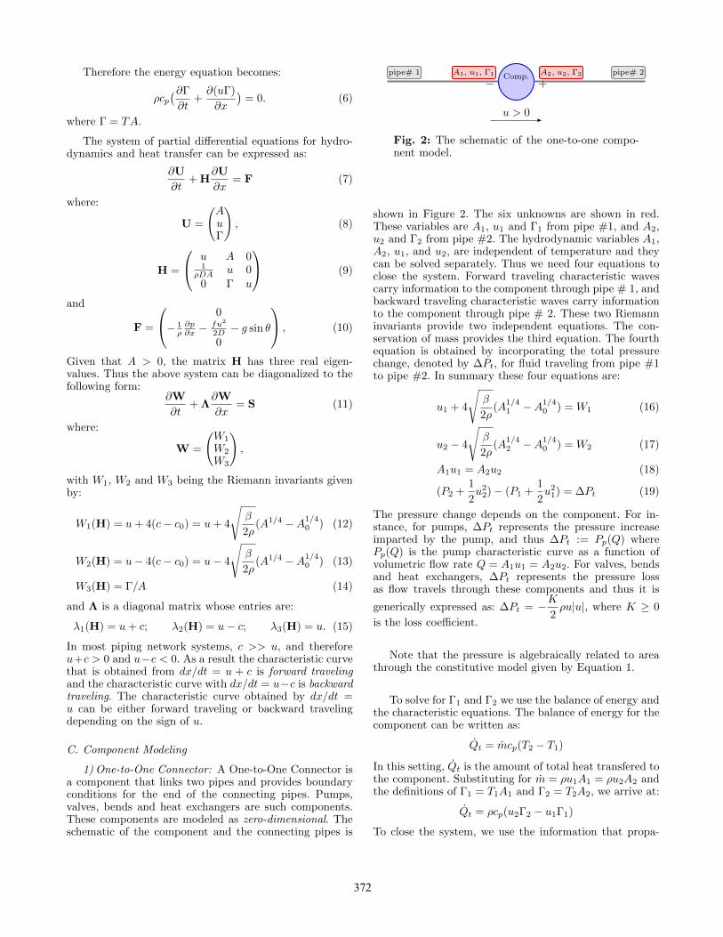
1) One-to-One Connector: A One-to-One Connector isa component that links two pipes and provides boundaryconditions for the end of the connecting pipes. Pumps,valves, bends and heat exchangers are such components.These components are modeled as zero-dimensional. Theschematic of the component and the connecting pipes is

Comp.pipe# 1 pipe# 2A1, u1, Γ1 A2, u2, Γ2

− +

u > 0

Fig. 2: The schematic of the one-to-one compo-nent model.

shown in Figure 2. The six unknowns are shown in red.These variables are A1, u1 and Γ1 from pipe #1, and A2,u2 and Γ2 from pipe #2. The hydrodynamic variables A1,A2, u1, and u2, are independent of temperature and theycan be solved separately. Thus we need four equations toclose the system. Forward traveling characteristic wavescarry information to the component through pipe # 1, andbackward traveling characteristic waves carry informationto the component through pipe # 2. These two Riemanninvariants provide two independent equations. The con-servation of mass provides the third equation. The fourthequation is obtained by incorporating the total pressurechange, denoted by ∆Pt, for fluid traveling from pipe #1to pipe #2. In summary these four equations are:

u1 + 4

√β

2ρ(A

1/41 −A1/4

0 ) = W1 (16)

u2 − 4

√β

2ρ(A

1/42 −A1/4

0 ) = W2 (17)

A1u1 = A2u2 (18)

(P2 +1

2u2

2)− (P1 +1

2u2

1) = ∆Pt (19)

The pressure change depends on the component. For in-stance, for pumps, ∆Pt represents the pressure increaseimparted by the pump, and thus ∆Pt := Pp(Q) wherePp(Q) is the pump characteristic curve as a function ofvolumetric flow rate Q = A1u1 = A2u2. For valves, bendsand heat exchangers, ∆Pt represents the pressure lossas flow travels through these components and thus it is

generically expressed as: ∆Pt = −K2ρu|u|, where K ≥ 0

is the loss coefficient.

Note that the pressure is algebraically related to areathrough the constitutive model given by Equation 1.

To solve for Γ1 and Γ2 we use the balance of energy andthe characteristic equations. The balance of energy for thecomponent can be written as:

Qt = mcp(T2 − T1)

In this setting, Qt is the amount of total heat transfered tothe component. Substituting for m = ρu1A1 = ρu2A2 andthe definitions of Γ1 = T1A1 and Γ2 = T2A2, we arrive at:

Qt = ρcp(u2Γ2 − u1Γ1)

To close the system, we use the information that propa-

372

gates along the characteristic dx/dt = u. This follows:

if u ≥ 0, T1 = W3

if u < 0, T2 = W3.

We assume that pumps, valves and bends are adiabaticand therefore Qt = 0 for these components. For heat ex-changers, i.e. heat loads and chillers, Qt is either calculatedfrom a reduced order model or it is assumed to be given.

2) One-to-Two Connector: One-to-two connector linksthree pipes at a junction. The modeling of a junction issimilar to the one-to-one connector with nine unknowns.The junctions could be of splitting or merging type. Formore details on the modeling of the junctions see reference[3].

D. Numerical Method

We use Discontinuous Galerkin (DG) method to dis-cretize the system of partial differential equations givenby equation 7. We split each pipe to Ne elements andwithin each element Legendre polynomials are used as thebasis. We use upwinded flux that propagates informationbetween the elemental regions and the bifurcations of thesystem. The equations for components form a nonlinearsystem of equations that are solved at every time stepusing the Newton-Raphson method. An Adams-Bashforthscheme is used for the time integration. A brief outline ofthe numerical method introduced in [3] is presented here.For more details on the numerical method see [4].

III. Demonstration case

In this section, we use the computational tool to an-alyze the performance of a cooling pipe network aboarda modern naval ship. In the following we describe theproblem inputs and the design parameters and then wediscuss the results.

A. Inputs

1) Geometric parameters: The overall length of theship is LS = 167.29(m), and the overall beam is LB =20.34(m). We place the coordinate system at the centerof the ship with the longitudinal coordinate, x, expandingfrom −LS/2 to LS/2.

2) Heat loads: There are 26 heat loads aboard the ship.We have considered the maximum values that the heatloads can acquire in different modes of operation. For thesake of simplicity, we have divided the ship into six equallongitudinal segments, or zones, and lumped all the loadsthat lie in each zone into a single load. The value of thelumped load is equal to the summation of all heat loadsthat lie within that segment, as shown in Table I.

3) Physical parameters: The Young’s modulus of thepipe is E = 1.84 × 1011(Pa), and the ratio of the pipediameter to its thickness is assumed to be D/e = 8 forall pipes. The bulk modulus of elasticity for water is K =2.39×1011(Pa). The density of water is ρ = 1028(kg/m3).The flow regime in all pipes is assumed to be turbulentand the friction factor is set to be constant at f = 0.04 forall pipes.

TABLE I: Lumped values of heat loads and theirlocations.

Identifier Q(kW ) x(m) y(m) z(m)

1 532 -66.67 -0.34 6.76

2 5050 -40.00 0.00 16.57

3 4723 -13.34 -0.08 18.27

4 2611 13.34 0.43 16.95

5 153 40.00 -2.00 5.41

6 378 66.67 2.00 0.01

B. Design variables

1) Thermal zones: Six thermal zones are considered,and two chillers are placed in each zone. The zonal bound-aries and chillers are shown in Figure 3.

2) Pipe configuration: A simple loop layout is consid-ered for the supply and return header; see [1] for moredetails and other options. The port and starboard mainpiping heights are 5.20 (m) and 10.20 (m), respectively.The offset between the supply and return header is 0.50(m).

The supply and return branch piping connect each heatload to the corresponding headers. We model each branchas a two-pipe segment with a single 90-degree bend in the(y − z) plane; all flow in the x direction occurs in theheaders.

3) Pipe/pump sizing: The pipe diameter for eachbranch is proportional to the corresponding heat load, Q.As an initial estimate, we use the parametric equationintroduced in reference [2]:

D = (4KQ

Cπ)0.4. (20)

The diameter is then rounded to the closest standard sizingfor pipes. The diameter of the main supply/return headeris Dh = 14 (inches). The supply pumps are located atthe exit of each chiller. Therefore we have a total of twelvepumps. The pumps are all identical with the characteristiccurve obtained from curve-fitting the empirical data asshown in Figure 4.

C. Results

We assume that the chilled water temperature is alwayskept constant at Tchill = 279.817K = 44F . This can beachieved by setting the temperature at chiller outlet at279.817K. Since we assume that the pipes are adiabatic,we expect to preserve this temperature in the supplypipes. In this fashion, we can measure the cooling capacityrequired at each chiller to always maintain the supplychilled water temperature at T = 279.817K. We initializethe temperature of all pipes at t = 0 to T = 279.817K.

In Figure 5, the coolant mass flow rate of three chillersversus time is shown. Chillers CH1 and CH2 both belong tothe same thermal zone, but due to the asymmetry of the

373

CH1

CH2

CH3

CH4

CH5

CH6

CH7

CH8

CH9

CH10

CH11

CH12

−80 −60 −40 −20 0 20 40 60 80

−10

0

10

x(m)y(m

)

Fig. 3: Double main piping system with branches (plan view). Zonal boundaries are shown with dashed greenline. the supply/return to heat loads are shown with gray line.

0 2 · 10−2 4 · 10−2 6 · 10−2 8 · 10−2 0.1 0.12 0.145

10

15

20

25

30

Q(m3/s)

H(m

)

Fig. 4: Pump characteristic curve chosen for thecoolant network. The circles show the empiricaldata provided by the pump manufacturer. Thesolid line shows a parabolic curve fit to the datapoints.

0 5 10 15 20 25 300

20

40

60

80

100

120

t(s)

m(kg/s)

CH1

CH2

CH7

Fig. 5: Chilled water mass flow rate at threedifferent chillers versus time.

pipe network, these two chillers have different mass flowrates. All three chillers show convergence to a steady stateafter a transient period. The “high-frequency” oscillationsobserved in the mass flow rate signal, are the result ofacoustic wave propagation throughout the pipe network.Since c >> u, these oscillations appear on much smallertime scales than the inertial time scale of the flow, i.e.D/u.

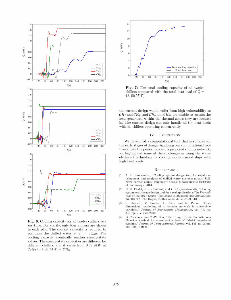
The primary objective of the current simulation is tocompute how much cooling capacity each chiller requiresto remove the heat from the loads in the steady operation.In Figure 6 the instantaneous cooling capacity of all twelvechillers are shown. For the sake of clarity, the plot is dividedinto three plots with four chillers shown in each plot. Thecooling capacity shown in Figure 6 represents the amountof heat that must be removed by each chiller to maintainthe supply water temperature at Tchill. As it is shown inFigure 6, each chiller experiences a sudden rise in Q, aftersome initial interval, which is due to the time it takes forthe return water to travel from the heat load back to thechillers. However, after the sudden rise, the demand forcooling capacity settles to the steady-state values.

Comparing the the total cooling capacity of all chillersversus the total heat load provides a robust verificationcheck for the numerical computation carried out in thissection. In Figure 7, the total cooling capacity of thecooling network is compared with the total heat load. Thetotal heat load is obtained by adding up the heat loadsgiven in table I. This value is Qload = 13.35(MW ). It isclear that the total cooling capacity converges to this value.

D. Analysis

The highest capacity is Q = 1.66(MW ) and it belongsto the third chiller. It is often preferred to choose identicalchillers for all thermal zones due to lower installationand maintenance costs. Thus for the current ship wewould need twelve chillers with the cooling capacity closeto 1.66(MW ), which is an order of magnitude increasecompared to conventional ships. A state-of-the-art chillerwith the cooling capacity of 1.5(MW ), has a volume of5.00(m)× 2.40(m)× 2.30(m) and it weighs 20000 kg. (Seefor instance York, Sea Water Cooled Centrifugal AC).Therefore the total volume and weight of the chillersroughly become 331 m3 and 24 tons. Moreover, a ship with

374

0 20 40 60 80 100 120 140 160 180 200 220−0.2

0

0.2

0.4

0.6

0.8

1

1.2

1.4

1.6

1.8

t(s)

Q(M

W)

CH1

CH2

CH3

CH4

0 20 40 60 80 100 120 140 160 180 200 220−0.2

0

0.2

0.4

0.6

0.8

1

1.2

1.4

1.6

1.8

t(s)

Q(M

W)

CH5

CH6

CH7

CH8

0 20 40 60 80 100 120 140 160 180 200 220−0.2

0

0.2

0.4

0.6

0.8

1

1.2

1.4

1.6

1.8

t(s)

Q(M

W)

CH9

CH10

CH11

CH12

Fig. 6: Cooling capacity for all twelve chillers ver-sus time. For clarity, only four chillers are shownin each plot. The coolant capacity is required tomaintain the chilled water at T = Tchill. Thecooling capacity eventually reaches steady-statevalues. The steady-state capacities are different fordifferent chillers, and it varies from 0.88 MW atCH12 to 1.66 MW at CH3.

0 20 40 60 80 100 120 140 160 180 200 2200

2

4

6

8

10

12

14

t(s)

Q(M

W)

Total cooling capacityTotal heat load

Fig. 7: The total cooling capacity of all twelvechillers compared with the total heat load of Q =13.45(MW ).

the current design would suffer from high vulnerability asCH7 and CH8, and CH9 and CH10 are unable to sustain theheat generated within the thermal zones they are locatedin. The current design can only handle all the heat loadswith all chillers operating concurrently.

IV. Conclusion

We developed a computational tool that is suitable forthe early stages of design. Applying our computational toolto evaluate the performance of a proposed cooling network,we highlighted some of the challenges in using the state-of-the-art technology for cooling modern naval ships withhigh heat loads.

References

[1] A. B. Sanfiorenzo, “Cooling system design tool for rapid de-velopment and analysis of chilled water systems aboard U.S.Navy surface ships,” Engineer’s thesis, Massachusetts Instituteof Technology, 2013.

[2] E. R. Fiedel, J. S. Chalfant, and C. Chryssostomidis, “Coolingsystem early-stage design tool for naval applications,”in Proceed-ings of the 2011 Grand Challenges in Modeling and Simulation,GCMS ’11, The Hague, Netherlands, June 27-29, 2011.

[3] S. Sherwin, V. Franke, J. Peiro, and K. Parker, “One-dimensional modelling of a vascular network in space-timevariables,” Journal of Engineering Mathematics, vol. 47, no.3-4, pp. 217–250, 2003.

[4] B. Cockburn and C.-W. Shu, “The Runge–Kutta discontinuousGalerkin method for conservation laws V: Multidimensionalsystems,” Journal of Computational Physics, vol. 141, no. 2, pp.199–224, 4 1998.

375