system integration and performance evaluation of …
TRANSCRIPT

SYSTEM INTEGRATION AND PERFORMANCE
EVALUATION OF WiNC2R PLATFORM FOR 802.11a
LIKE PROTOCOL
BY MADHURA JOSHI
A Thesis submitted to the
Graduate School -- New Brunswick
Rutgers, The State University of New Jersey
in partial fulfillment of the requirements
for the degree of
Master of Science
Graduate Program in Electrical and Computer Engineering
Written under the direction of
Dr. Predrag Spasojevic
and approved by
_________________________________
_________________________________
_________________________________
_________________________________
New Brunswick, New Jersey
October 2010

© 2010
Madhura Joshi
ALL RIGHTS RESERVED

ii
ABSTRACT OF THE THESIS
System Integration and Performance Evaluation of WINLAB Network Centric Cognitive Radio Platform for
802.11a Like Protocol
By Madhura Joshi
Thesis Director: Prof. Predrag Spasojevic
A Cognitive Radio (CR) is an intelligent transceiver that is able to support
multiple technologies. It can also be dynamically reconfigured and be easily
programmed to achieve high flexibility and speed.
The WiNC2R platform is based on the concept of Virtual Flow Paradigm. The key
characteristic of this concept is that the software provisions the flow by
determining the roles of hardware and software modules whereas the runtime
processing flow is controlled by the hardware. The revision1 of WiNC2R platform
was a proof of concept implemented on an FPGA with the basic processing
engines to achieve an 802.11a-light OFDM flow, and a simple Virtual Flow
Pipeline (VFP) control unit. In the new revision, we have an advanced shared
VFP control unit, cluster based SoC architecture, and all the processing engines
in an 802.11a like OFDM transmitter flow.
The focus of this thesis was to integrate the WiNC2R platform as an 802.11a like
transmitter with the advanced VFP control unit and perform a performance
analysis for the realistic application scenario. The performance evaluation
revolves around system throughput and latency as a function of frame size,

iii
bandwidth, pipelining granularity, number of traffic flows, and flow bandwidth.
The analysis is performed for various traffic mix scenarios. We analyze also how
effectively the VFP control scheme performs run time task control for a single
and multiple OFDM flows.
The thesis starts with the comparative study between the two revisions of
WiNC2R and continues to describe in detail the new revision features. The
programming techniques are described next, followed by a performance
evaluation section and suggestions for future work.

iv
ACKNOWLEDGEMENTS
I would first like to thank my parents for their constant support without which my
journey of completing the MS degree would not have been possible. I would like
to thank my advisors Prof. Predrag Spasojevic and Prof. Zoran Miljanic for their
time and guidance during the course of completing my thesis. Their advice and
suggestions have proven to be very helpful in successfully accomplishing my
task. I would also like to thank Ivan Seskar for his support despite being on a
very busy schedule.
Being a part of the WiNC2R team has been a fun experience, which would not
have been possible without Onkar, Akshay and Mohit. I would like to thank them
from the bottom my heart, and I will truly miss working with them. I would also
like to thank Khanh, Sumit, Tejaswy, Renu and Prasanthi who have always
helped me to resolve my doubts.

v
Table of Contents ABSTRACT OF THE THESIS .............................................................................. ii
ACKNOWLEDGEMENTS.................................................................................... iv
Table of Contents ................................................................................................ v
List of Abbreviations........................................................................................ viii
List of Tables ...................................................................................................... ix
List of Figures...................................................................................................... x
CHAPTER 1 .......................................................................................................... 1
INTRODUCTION................................................................................................... 1
1.1 Classification of CR Platforms ............................................................................ 2
1.2 WINLAB Network Centric Cognitive Radio Platform......................................... 3
CHAPTER 2 .......................................................................................................... 6
Cluster Based WiNC2R Architecture................................................................. 6
2.1: WiNC2R Revision 1 Architecture ....................................................................... 6
2.1.1: Functional Unit Architecture............................................................................ 8
2.1.2: WiNC2R Revision 1 Shortcomings ............................................................... 11
2.2: WiNC2R Revision2 Architecture ...................................................................... 12
2.2.1 WiNC2R Revision1 Memory Map .................................................................. 16
2.2.2: WiNC2R Revision2 System Memory Map .................................................... 18
2.2.2: VFP Memory Map ......................................................................................... 20
2.2.3: General FU Memory Map ............................................................................. 21

vi
2.2.4: Tensilica FU Memory Map ............................................................................ 22
2.3: AMBA Advanced eXtensible Interface (AXI) ................................................... 23
2.3.1: Read Burst Transaction ................................................................................ 25
2.3.2: Write Burst Transaction ................................................................................ 26
2.3.3 AXI Bus Configuration Parameters ................................................................ 28
CHAPTER 3 ........................................................................................................ 33
WiNC2R Revision2 Programming Flow........................................................... 33
3.1 GTT, TD and NTT Interface ................................................................................ 33
3.2 Input Buffer and Output Buffer Indexing.......................................................... 34
3.2.1 Input Buffer .................................................................................................... 35
3.2.2 Output Buffer.................................................................................................. 36
3.3 System Flow........................................................................................................ 37
3.4 Task Scheduling ................................................................................................. 39
3.4.1 Concept of Chunking ..................................................................................... 40
Chapter 4............................................................................................................ 43
WiNC2R Revision 2 Processing Engines........................................................ 43
4.1: 802.11a Protocol Description ........................................................................... 43
4.1.1:PLCP Frame Format...................................................................................... 44
4.2: 802.11a TRANSMITTER..................................................................................... 49
4.3 WiNC2R 802.11a Transmitter Flow: .................................................................. 50
4.3.1: GNU Radio.................................................................................................... 51
4.3.2: Integrating GNU functions in WiNC2R.......................................................... 51
4.3.3: Direct Programming Interface ....................................................................... 51
4.3.4: Implementation ............................................................................................. 52

vii
4.3.5: Compiling ...................................................................................................... 53
4.4: WiNC2R Processing Engine Specifications.................................................... 54
CHAPTER 5 ........................................................................................................ 61
Performance Evaluation of WiNC2R................................................................ 61
5.1 WiNC2R Test – Bench Using OVM .................................................................... 61
5.1.1 Basic Experiment ........................................................................................... 63
5.1.2 System Latency Experiment .......................................................................... 68
5.1.3 Variation of chunk size on system latency ..................................................... 70
5.1.4 Evaluation of Multiple Flow Support by VFP.................................................. 71
CHAPTER 6 ........................................................................................................ 78
CONCLUSION AND FUTURE WORK ............................................................... 78
Bibliography ...................................................................................................... 80

viii
List of Abbreviations
CR: Cognitive Radio
WiNC2R: WINLAB Network Centric Cognitive Radio
VFP: Virtual Flow Pipeline
FU: Functional Unit
PE: Processing Engine
PLB: Processor Local Bus
AXI: Advanced eXtensible Interface
OVM: Open Verification Environment
DPI: Direct Programming Interface
SV: System Verilog

ix
List of Tables Table 2-1: AXI Core Configuration Parameters................................................... 32
Table 4-1: Rate Field Encoding........................................................................... 46
Table 4-2: ChunkSize Calculation ....................................................................... 56
Table 5-1: System Throughput............................................................................ 68
Table 5-2: Variation of latency with chunksize .................................................... 71
Table 5-3: Throughput for two flows.................................................................... 77

x
List of Figures
Figure 2-1: WiNC2R Revision1 Architecture ......................................................... 6
Figure 2-2: Functional Unit Architecture................................................................ 8
Figure 2-3: WiNC2R Revision2 Architecture ....................................................... 13
Figure 2-4: VFP Processing Flow........................................................................ 15
Figure 2-5: WiNC2R revision1 memory map....................................................... 16
Figure 2-6: WiNC2R revision1 FU memory map................................................. 17
Figure 2-7: WiNC2R Base Address Calculation.................................................. 19
Figure 2-8: WiNC2R System Memory Map......................................................... 20
Figure 2-9: AXI Read Channel Architecture ........................................................ 23
Figure 2-10: AXI Write Channel Architecture ...................................................... 24
Figure 2-11: AXI Read Burst Transaction ........................................................... 25
Figure 2-12: AXI Write Burst Transaction............................................................ 26
Figure 3-1: GTT, TD and NT table interface........................................................ 34
Figure 3-2: Input Buffer Partitions ....................................................................... 35
Figure 3-3: Output Buffer Partitions..................................................................... 36
Figure 3-4: System Flow ..................................................................................... 39
Figure 4-1: PPDU Frame Format ........................................................................ 45
Figure 4-2: OFDM Training Sequence ................................................................ 45
Figure 4-3: 802.11a Transmitter.......................................................................... 49
Figure 4-4: WiNC2R 802.11a Transmitter........................................................... 50
Figure 4-5: WiNC2R System Hierarchy............................................................... 53
Figure 4-6: Data Scrambler ................................................................................. 57

xi
Figure 4-7: Convolutional Encoder (Constraint Length 7) ................................... 59
Figure 5-1: WiNC2R Verification Environment .................................................... 62
Figure 5-2: Single Flow Data Transfer ................................................................ 63
Figure 5-3: WiNC2R Transmitter Frame Flow..................................................... 64
Figure 5-4: Single Flow Latency.......................................................................... 69
Figure 5-5: Multiple Flow Data Transfer .............................................................. 73
Figure 5-6: Multiplexing of chunks in 2 flows....................................................... 73
Figure 5-7: Variation in latency between single and two flows at rate 6Mbps..... 75
Figure 5-8: Variation in latency between single and two flows at rate 12Mbps... 76
Figure 5-9: Variation in latency between single and two flows at rate 24Mbps... 76

1
CHAPTER 1
INTRODUCTION
The next generation wireless technologies clearly impose heterogeneity in their
infrastructures, with devices using different radio access technologies and
operating at different spectrum bandwidths. (1)Emerging wireless technologies
call for solutions with frequent spectrum sensing in addition to per packet
adaption of interference, adaption of frequency bands, and yet remain power
friendly.
Simultaneous support of such diverse traffic streams and dynamic adaption
drives the need of virtualization that can guarantee proper sharing of resources,
yet maintaining the end to end latency requirements for each flow.
Cognitive Radio (CR) platforms strive to achieve adaptability, inter-operability
and efficient spectrum usage at fast data rates. The following section describes
some of the cognitive radio platforms in brief.

2
1.1 Classification of CR Platforms
The current CR platforms are classified into four types(2)(3).
1. Multimodal Hardware-based Platforms: These platforms implement
different technologies by implementing separate modules that support a
particular technology. Once programmed, the modules cannot be
reprogrammed to implement a different MAC protocol or modify the
system parameters. Thus, this type of platform lacks the re-configurability
of an ideal cognitive radio. Also, this kind of platform is not scalable, as
new modules need to be implemented to support more number of
technologies.
2. Portable Software Platforms: These platforms implement the radio
functionalities in a high level programming language such as C, C++ or
JAVA. As the modules are implemented in software, they are easily re-
configurable and also scalable to support multiple technologies. These
platforms run as application software on a general purpose or real time
operating system on a general-purpose processor. Since RF
functionalities such as filtering, up/down conversion, analog to digital
conversion and digital to analog conversion are cumbersome to implement
in software, RF boards are used to provide a wireless interface. The GNU
Radio is one such portable software platform. The performance of these
platforms depends on the general purpose processor and the underlying
operating system.

3
3. Reconfigurable Hardware Platforms: These platforms implement the
physical and the MAC layer functions in FPGA blocks or a combination of
FPGA and DSP processor. The platform can support either one or a
limited number of protocols, but can be re-configured to support a different
protocol by uploading a different bit image onto the FPGA. The modules
performing the radio functions are implemented either in low-level
hardware or embedded languages and hence difficult to program. The
performance of these platforms is limited by the logic capacity of FPGA
and the clock rates supported by FPGA and DSP processors. The RICE
university WARP platform is one such platform.
4. SoC Programmable Radio Processors: These platforms are based on an
array of special purpose processors and hardware accelerators for
implementing physical layer radio functions. The MAC and the physical
layer functions are software programmable. There is no underlying
operating system like in the case reconfigurable platforms. The
performance of these platforms mainly depends on the number of the
processors used and the choice of hardware accelerators.
1.2 WINLAB Network Centric Cognitive Radio Platform
The WINLAB Network Centric Cognitive Radio (WiNC2R) is a platform that
targets speed, simple programming and flexibility in the multilayer domain of
mobile IP based communication. Its goal is to provide a scalable and adaptive
radio platform for the range of cost-capacity configurations, so the architecture is

4
suitable for both standard cell SoC and FPGA based implementations. The
WiNC2R is an excellent platform for the research and development
communication labs in academia, industry and government institutions. It can be
used for the analysis of the mobile applications computing, communication and
control requirements, performance analysis of communication algorithms in a
realistic radio propagation environments and hardware versus software
implementation tradeoff analysis. This paradigm introduces the concept of Virtual
Flow pipelining (VFP) which combines the high-speed computation capabilities of
FPGA hardware and flexibility of software. The data flow and parameter inputs to
processing blocks are fed by the user in the form of function calls, but the
processing happens on hardware. The WiNC2R board is differentiated from the
other cognitive radio projects in the sense that the design uses hardware
accelerators to achieve programmability and high performance at each layer of
the protocol stack.
The WiNC2R revision1 framework was a successful proof of concept
implementation on an FPGA. The framework consisted of basic 802.11a
processing elements and a low level VFP controller. The transmitter and receiver
were implemented on separate FPGA’s and successful transmission and
reception of packets was achieved. The next revision of WiNC2R is targeted
towards an ASIC implementation and hence is a re-configurable SoC based
architecture. This revision aims to achieve successful transmission and reception
of 802.11a frames with the advanced VFP controller for scalable SoC solutions.
The following chapters describe a comparative analysis between the two

5
frameworks, in detail description of different processing engines and an
evaluation of the new framework.

6
CHAPTER 2
Cluster Based WiNC2R Architecture
2.1: WiNC2R Revision 1 Architecture
Figure 2-1: WiNC2R Revision1 Architecture
The above figure shows the top-level architecture of WiNC2R (revision 1).
The architecture can be split into two main sections – software and hardware.

7
The upper block represents the software components that perform the task of
initial configuration of the system. Since WiNC2R revision1 was FPGA based
architecture, the CPU core used on the software side was a standard Xilinx soft-
core CPU called Microblaze which connected to its own GPIO ports (General
Purpose IO), Timer and Interrupt peripheral modules using an IBM standard bus
structure called Processor Local Bus (PLB). The hardware components are
initialized and the data flow between them was configured through software. The
lower block represents the hardware components that perform the actual radio
processing tasks. The data processing occurs in the Functional Units (FU) and
the data transfer from one FU to another occurs over the PLB. All FU’s were
implemented in VLSI Hardware Description Language (VHDL). The FU interfaces
to the PLB through Xilinx standard Intellectual Property Interface (IPIF).

8
2.1.1: Functional Unit Architecture
Figure 2-2: Functional Unit Architecture
The FU consists of Processing Engine (PE), VFP controller, input and
output memories as shown in the above figure. The operations performed by an
FU are split into two categories – data and control. The data operation refers to
the data processing handled by the PE, while the control operation refers to the
tasks performed by the VFP controller to initiate and terminate the PE tasks. The
inputs required by the PE for data processing is stored in the input memory
buffer, while the data generated after processing is stored in the output memory
buffer. The memory buffers are implemented as Dual Port Random Access
Memory (DPRAM) generated using Xilinx CoreGen. The Register MAP (RMAP)

9
within the PE stores software configurable control information required for PE
processing.
The VFP controller manages the operation of FU-s achieving re-
configurability. WiNC2R uses a direct architectural support for task-based
processing flow. The task flow programming is performed by two control data
structures: Global Task-descriptor Table (GTT) and Task-Descriptor Table (TD
Table). Both control tables are memory based. GTT was implemented as a block
RAM connected to the PLB and common to all FUs while each FU had its own
TD Table. Based on its core functionality, each PE was assigned a set of input
tasks and the PE was idle until it received one of those tasks. The PE handles
two types of tasks: data and control. Data task indicated that data to be
processed was present in the input buffer of the PU. For example, data task
“TxMod” told the Modulator block that there was data in the input buffer that
needed to be modulated. This data was first transferred to the input buffer of FU
before the task was sent to the PE. Control tasks do not operate on the payload
but behave as pre-requisites for data tasks in some PE’s. For example,
“TxPreambleStart” control command initiated the preamble generation task in the
PE_TX_IFFT engine before handling a data task. This was necessary, as the
preamble is attached to the beginning of the data frame before transmitting.
The TD Table stores all the required information for each task for the FU.
When the FU received a data task, the VFP controller Task Activation (TA) block
fetches the information from the TD table and processes it. It then forwards the
task to PE along with the location and size of input data. The PE processed the
data and stored it in the Output Buffer. Once the processing was over, PE

10
relayed the location and size of processed data in Output Buffer to the VFP
controller through Next Task Request and Next Task Status signals. The Next
Task Status bits indicate the location of the processed data in the output buffer.
Depending on the PU, the output data may be stored at more than one location.
The Next Task Request signal informs the VFP controller Task Termination (TT)
block how the output data at locations indicated by status bits should be
processed. The TT processing includes transferring the data to next FU/FUs in
the data flow. The NT Request tells the TT to which FU the data is to be sent.
The FU in the data flow in determined by the information stored in TD table. By
updating the information in TD table, software can change the next FU in the
data flow path. Thus, the PE has no information regarding the next processing
engine in the flow. As a result, all the PE’s are independent of each other and
only perform the tasks allocated to them. The next processing engine in the flow
can thus be changed on-the-go and hence a complete reconfigurable
architecture is achieved.
11
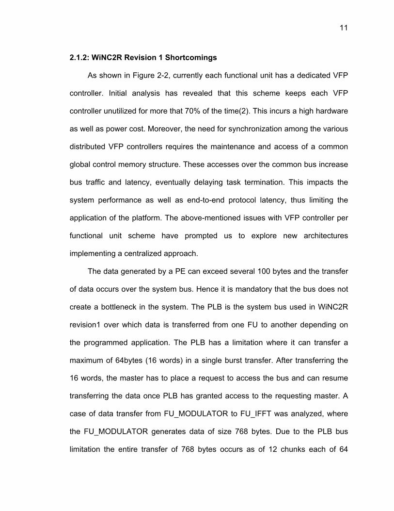
2.1.2: WiNC2R Revision 1 Shortcomings
As shown in Figure 2-2, currently each functional unit has a dedicated VFP
controller. Initial analysis has revealed that this scheme keeps each VFP
controller unutilized for more that 70% of the time(2). This incurs a high hardware
as well as power cost. Moreover, the need for synchronization among the various
distributed VFP controllers requires the maintenance and access of a common
global control memory structure. These accesses over the common bus increase
bus traffic and latency, eventually delaying task termination. This impacts the
system performance as well as end-to-end protocol latency, thus limiting the
application of the platform. The above-mentioned issues with VFP controller per
functional unit scheme have prompted us to explore new architectures
implementing a centralized approach.
The data generated by a PE can exceed several 100 bytes and the transfer
of data occurs over the system bus. Hence it is mandatory that the bus does not
create a bottleneck in the system. The PLB is the system bus used in WiNC2R
revision1 over which data is transferred from one FU to another depending on
the programmed application. The PLB has a limitation where it can transfer a
maximum of 64bytes (16 words) in a single burst transfer. After transferring the
16 words, the master has to place a request to access the bus and can resume
transferring the data once PLB has granted access to the requesting master. A
case of data transfer from FU_MODULATOR to FU_IFFT was analyzed, where
the FU_MODULATOR generates data of size 768 bytes. Due to the PLB bus
limitation the entire transfer of 768 bytes occurs as of 12 chunks each of 64

12
bytes.
The above-mentioned shortcomings of WiNC2R revision1 architecture led
us to explore different options to overcome the shortcomings. Centralizing the
VFP controller for several FU’s and using a system bus of better throughput such
as AMBA AXI, are the highlights of the WiNC2R revision2 architecture.
2.2: WiNC2R Revision2 Architecture
WiNC2R revision2 is a Cluster Based System on Chip architecture (SoC) as
shown in the Figure 2-3. The system interconnect used in revision2 architecture
is AMBA AXI. Hierarchical bus architecture is implemented as shown in Figure 2-
3. The communication between the clusters occurs over the main system bus
while the communication between the FU’s within a cluster occur over another
AXI bus within a cluster. The dedicated VFP controller in the previous
architecture is replaced with a VFP Controller that is common to several FU’s
within a cluster. The architecture of the FU is similar to the one in revision1
architecture consisting of a dedicated processing engine, input, output buffer
memories and a Dynamic Memory Access (DMA) Engine to transfer data
between FU’s over the AXI bus present with a cluster. The communication
between the VFP controller and FU’s occur over a dedicated bus to each FU. As
in the previous architecture, the PE handles both the data and the control tasks
while the VFP controller schedules the tasks to each FU.

13
Figure 2-3: WiNC2R Revision2 Architecture
Source: Onkar Sarode, Khanh Le, Predrag Spasojevic, Zoran Miljanic: Scalable Virtual Flow
Pipelining SoC Architecture, IAB Fall 2009 Poster

14
The VFP controller’s functions are divided into – task scheduling and
activation, communication between the tasks and scheduling of processing
resources to the tasks. The task activation function includes dynamically
scheduling a task, identifying the FU corresponding to the task and initiating it.
The Task Activation (TA) block that is local to every FU performs the actual
initiation of a task. Once the VFP activates a particular FU, it is free to perform
task activation of other FU’s. Once the PE within an FU completes processing
the data, it activates the task termination blocks within the VFP. The Next Task
Table (NTT) within the VFP contains information regarding the task to be
performed next. Hence, the VFP initiates the data transfer between the producer
and consumer FU. The consumer FU can be placed either in the same (local)
cluster or a different (remote) cluster. If the consumer FU is present in the local
cluster, the data transfer occurs over the AXI bus within the cluster. But if the
consumer FU is present in a remote cluster, the data transfer occurs over the
system-interconnect.

15
Figure 2-4: VFP Processing Flow
Source: Onkar Sarode, Khanh Le, Predrag Spasojevic, Zoran Miljanic: Scalable Virtual Flow
Pipelining SoC Architecture, IAB Fall 2009 Poster
Due to centralization of the VFP and a cluster-based architecture, the
decoding scheme to identify a particular FU is different from the revision1
architecture. The following section describes the WiNC2R revision1 and
revision2 memory maps in detail.
16
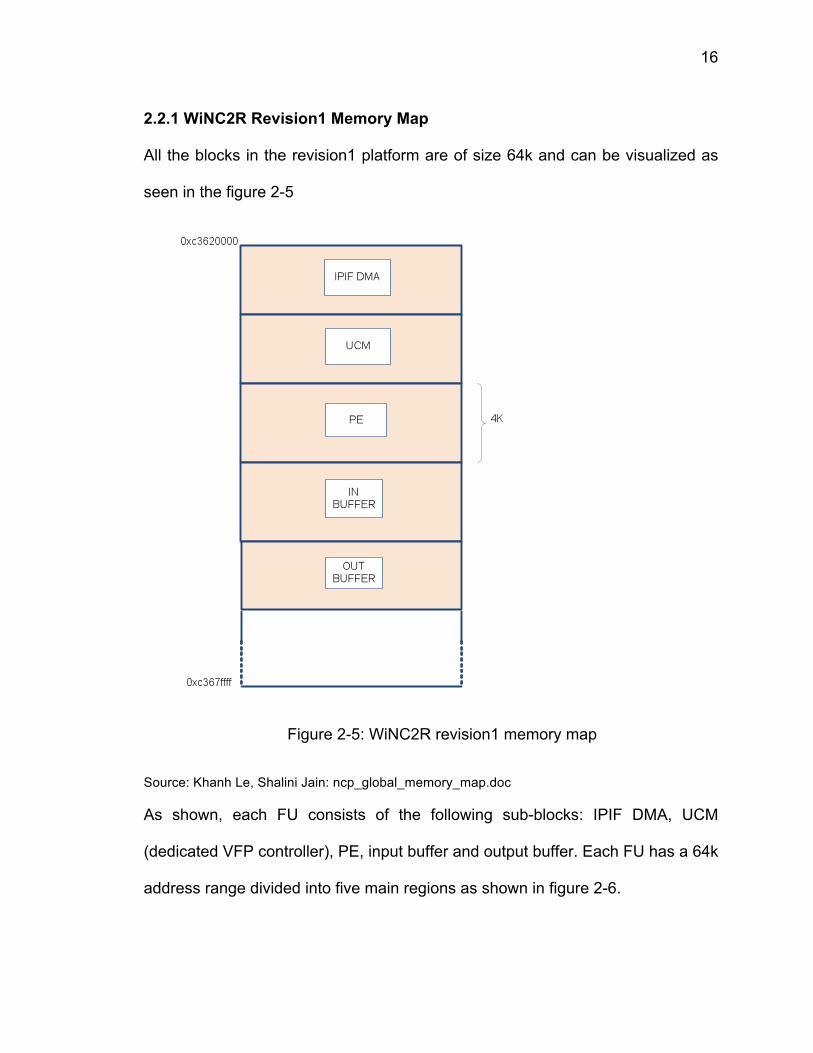
2.2.1 WiNC2R Revision1 Memory Map
All the blocks in the revision1 platform are of size 64k and can be visualized as
seen in the figure 2-5
Figure 2-5: WiNC2R revision1 memory map
Source: Khanh Le, Shalini Jain: ncp_global_memory_map.doc
As shown, each FU consists of the following sub-blocks: IPIF DMA, UCM
(dedicated VFP controller), PE, input buffer and output buffer. Each FU has a 64k
address range divided into five main regions as shown in figure 2-6.

17
Figure 2-6: WiNC2R revision1 FU memory map
Source: Khanh Le, Shalini Jain: ncp_global_memory_map.doc
Since, each FU has a dedicated VFP controller, address decoding of the different
FU’s is based only their base memory address. Secondly, each FU has its own
TD table and Task Scheduler Queue.
Due a centralized VFP controller in the new revision, the address decoding of the
different FU’s is based on an FU_ID and CLUSTER_ID. These id’s allow the VFP

18
controller to identify a particular FU. This feature was unnecessary in the
previous revision because of a dedicated VFP controller.
2.2.2: WiNC2R Revision2 System Memory Map
The WiNC2R revision2 architecture has a maximum of 16 clusters and each
cluster can have a maximum of 16 FU’s.
Size of 1 FU = 512KB
Size of 1 Cluster = 16 * 512KB = 8MB
Size of 16 Clusters = 16 * 8MB = 128MB.
Hence, the total system memory is of size 128MB. The base address of each
cluster and the decoding of the FU address are shown in figure 2-7.
To access a memory space of 128MB, we require 27bits. Its “Cluster ID”
identifies the cluster while the FU is identified by its “FU ID”. The cluster and FU
ID are 4 bits wide. As shown, the bits 26 to 23 represent the cluster ID and bits
22 to 19 represent the FU ID. For example, the base address of FU 1 in cluster 0
is 0x0008000.

19
Figure 2-7: WiNC2R Base Address Calculation
Source: Akshay Jog, Khanh Le: WiNC2R Global Memory Map – Release 2
The revision2 framework consists of certain new FU’s in addition to the FU’s from
the revision1 architecture. The processing engine within the FU is either a native
C/C++ function from GNU Radio or a SystemC wrapped Tensilica Application
Specific Instruction Set Processor Entity or a VHDL entity from revision1
architecture. Figure 2-8 represents the VFP, General FU and Tensilica based FU
memory map. The base address of each memory entity is also shown.

20
Figure 2-8: WiNC2R System Memory Map
Source: Akshay Jog, Khanh Le: WiNC2R Global Memory Map – Release 2
2.2.2: VFP Memory Map
Since the VFP is a centralized entity controlling several FU’s, certain
memories that were local to an FU in the previous architecture are now a
common memory entity in the VFP.
Global Task Table (GTT): The GTT is a 64KB memory that resides within
the VFP. Since the GTT is local to VFP, there is one GTT per cluster. The GTT
describes the flow of tasks depending on the application. The GTT was a global
memory table in the revision 1 framework and hence was common to all FU’s .
Task Scheduler Queue (TSQ): Each FU in the revision 1 framework had a
local TSQ. Depending on the nature of the task, the task descriptors were either
stored in the synchronous or the asynchronous queues. Since the common VFP
controller handles the scheduling of tasks of different FU’s, the TSQ is now made

21
local to the VFP rather than having a separate TSQ in each FU.
To begin with, it is assumed that a cluster consists of 8 FU’s. Hence the
128KB memory space of TSQ is divided into 8 resulting in a 16KB TSQ per FU.
The tasks corresponding to every FU is placed in the appropriate TSQ by the
VFP controller.
VFP RMAP: The VFP controller can be initialized by the software by writing
into the VFP RMAP. Currently the VFP RMAP is not used.
Next Task Table (NTT): The NTT contains information regarding the next
task to be activated the VFP after the completion of a particular task by the FU.
This information previously resided in the TD table that was local to each FU. It is
now stored in a different memory entity and is local to the VFP.
2.2.3: General FU Memory Map
The general FU memory map is similar to the one in the previous revision,
except for some minor changes that are described below.
PE RMAP: The processing engine can be configured and initialized by
writing into its RMAP. The software writes into the RMAP during system
configuration.
PE IBUF: The PE IBUF is divided into two sections – the IBUF and the TD
table. The PE reads the required data for it’s processing from the PE IBUF, while
the TD table consists of information that describe the task being performed.
Hence each FU has a local TD table describing the tasks that the particular FU
can perform.

22
PE OBUF: After processing the data read from IBUF, the PE writes the data
into the OBUF. When the VFP controller initiates a DMA transfer, the data from
the OBUF is transferred into the IBUF of the FU that is next in processing flow.
2.2.4: Tensilica FU Memory Map
Instruction RAM (IRAM): The Instruction RAM stores the instruction set
required for the processor to execute the data processing algorithm.
Data RAM (DRAM): The Data RAM stores the variables required by the
processor to execute the data processing algorithm.
The data stored in PE RMAP,IBUF and OBUF is similar to the one
described in the general FU memory map section.
The second bottleneck in the revision 1 framework was created by the PLB. We
decided to replace the PLB with the AMBA AXI bus. The following section
describes the AXI bus in detail.

23
2.3: AMBA Advanced eXtensible Interface (AXI)
The AMBA AXI bus extends the AMBA Advanced High performance Bus
(AHB) with advanced features to support next generation high performance SoC
architectures. The AXI bus has channel architecture and can be configured to
have separate write and read address and data channels. The AXI architecture
for read and write requests is shown in Figure 2-7 and Figure 2-8.
Figure 2-9: AXI Read Channel Architecture
24
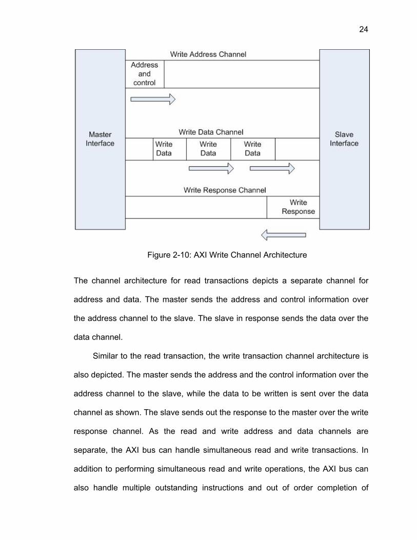
Figure 2-10: AXI Write Channel Architecture
The channel architecture for read transactions depicts a separate channel for
address and data. The master sends the address and control information over
the address channel to the slave. The slave in response sends the data over the
data channel.
Similar to the read transaction, the write transaction channel architecture is
also depicted. The master sends the address and the control information over the
address channel to the slave, while the data to be written is sent over the data
channel as shown. The slave sends out the response to the master over the write
response channel. As the read and write address and data channels are
separate, the AXI bus can handle simultaneous read and write transactions. In
addition to performing simultaneous read and write operations, the AXI bus can
also handle multiple outstanding instructions and out of order completion of

25
transactions. The read and write transaction protocols are described below.
2.3.1: Read Burst Transaction
Figure 2-11: AXI Read Burst Transaction
Source: AMBA AXI v1.0 Specifications
The above figure represents a read burst transaction.(4)
• The master asserts the “arvalid” signal along with a valid address on
the “araddr” signal.
• The slave asserts the “arready” signal, indicating that the slave is
ready to accept the address and the corresponding control signals.
• The master asserts the “rready” signal, indicating to the slave that it is
ready to accept the data and the responses.
• The slave asserts the “rvalid” signal along with the valid data on the
“rdata” signal. The slave indicates the master that the data on the
“rdata” signal is the last in the burst transaction by asserting the
“rlast” signal.

26
2.3.2: Write Burst Transaction
Figure 2-12: AXI Write Burst Transaction
Source: AMBA AXI v1.0 Specifications
The above figure represents a write burst transaction.(4)
• The master the “awvalid” signal along with a valid address on the
“awaddr” signal.
• The slave asserts the “awready” signal, which indicates that the slave
is ready to accept the address and other control signals.
• The slave asserts the “wready” signal, which indicates that the slave is
ready to accept the data.
• The master then asserts the “wvalid” signal and also puts valid data on
the “wdata” signal. Along with this, the master also asserts the
“bready” signal indicating that it is ready to accept the response from
the slave.

27
• The master asserts the “wlast” signal along with the “wvalid” and
“wdata” signal, indicating that the word is the last word in the burst
transaction.
• The slave sends back the response on the “bresp” signal along with
asserting the “bvalid” signal, indicating that the response on “bresp”
channel is valid.
The maximum number of data transfer in a burst is defined by the “awlen” or
“arlen” signal. The signal can be configured to have a maximum of 256-byte
transfer in a single burst. This provides an improved performance over the PLB,
which handles only 64-byte transfer in a single burst transaction. The size of data
in each burst is configured by the “awsize” and “arsize” signals and is set as 32
bit word. The AXI bus can perform burst transfers of 3 kinds.
• Fixed Burst: In a fixed burst, the address remains the same for every
transfer in the burst. This burst type is for repeated accesses to the
same location such as when loading or emptying a peripheral FIFO.
• Incremental Burst: In an incrementing burst, the address for each
transfer in the burst is an increment of the previous transfer address.
The increment value depends on the size of the transfer. For
example, the address for each transfer in a burst with a size of four
bytes is the previous address plus four.

28
• Wrap Burst: A wrapping burst is similar to an incrementing burst, in
that the address for each transfer in the burst is an increment of the
previous transfer address. However, in a wrapping burst the address
wraps around to a lower address when a wrap boundary is reached.
The wrap boundary is the size of each transfer in the burst multiplied
by the total number of transfers in the burst.
2.3.3 AXI Bus Configuration Parameters
The AXI bus core is configured using Synopsys DesignWare CoreConsultant.
There are various design parameters that determine the behavior of the AXI
core. Some of the parameters that are relevant to the system are mentioned in
the table below.

29
AXI Core
Parameter
Parameter Definition Configuration
Chosen
Reason
AXI Data Bus
Width
This is the width of the data bus
that applies to all interfaces.
Legal values: 8, 16, 32, 64, 128,
256 or 512 bits
32 bits Standard data
size width
AXI Address Bus
Width
This is the width of the address
bus that applies to all interfaces.
Legal values: 8, 16, 32, 64, 128,
256 or 512 bits
32 bits Standard address
size width
Number of AXI
Masters
Number of masters connecting
the to AXI master port.
Maximum value = 16
9 System consists
of 7 functional
units, 1 VFP
controller and
OVM
environment. All
act as masters
Number of AXI
slaves
Number of slaves connecting to
the AXI slave port
8 The 7 functional
units and VFP act
as slaves
AXI ID: Width of
Masters
(AXI_MIDW)
This is the ID bus width of all five
AXI channels connected to an
external master. All masters have
the same ID width for all five AXI
channels.
4 4 bits are
sufficient to
access 9 masters
AXI ID: Width of
Slaves
This is the ID bus width of all five
AXI channels connected to an
8 Generated
automatically

30
(AXI_SIDW) external slave. It is a function of
the AXI ID Width of Masters
(AXI_MIDW) and the number of
masters (AXI_NUM_MASTERS).
AXI_SIDW=AXI_MIDW
+ceil(log2(NUM_AXI_MASTERS))
This parameter is calculated
automatically, and the same width
is applied to all slaves.
using the
mentioned
formula
AXI Burst Length
Width
This is the width of the burst
length signal for both read and
write address channels on both
the master and slave ports. The
AXI protocol specifies this is a 4
bit value, but this width is
configurable to 8 bits wide to
support longer bursts up to 256
data beats.
8 bits Maximum value of
burst length width
is selected to
enable the
transfer of 256
words in a single
burst.
Slave Port
Arbiters (read
address, write
address and write
data channels)
Selects the type of arbiter to be
used at the slave port read
address, write address and write
data channels.
Priority Arbitration: Highest
priority master wins
First Come First Serve: Masters
are granted access in the order of
the incoming requests.
Fair Among Equals – 2 tier
First Come First
Serve
All the slaves are
of equal priority
and hence first
come first is
chosen

31
arbitration: First tier is dynamic
priority; second tier shares grants
equally between masters of the
same highest requesting priority
on a cycle-by-cycle basis.
User Defined: instantiates a plain-
text arbitration module which the
user can edit to their own
requirements
Master Port
Arbiters ( read
data channel and
burst response
channel)
Selects the type of arbiter to be
used at the master port read data
and burst response channels.
Priority Arbitration: Highest
priority master wins
First Come First Serve: Masters
are granted access in the order of
the incoming requests.
Fair Among Equals – 2 tier
arbitration: First tier is dynamic
priority; second tier shares grants
equally between masters of the
same highest requesting priority
on a cycle-by-cycle basis.
User Defined: instantiates a plain-
text arbitration module which the
user can edit to their own
requirements
First Come First
Serve
All the masters
are of equal
priority and hence
first come first is
chosen

32
Table 2-1: AXI Core Configuration Parameters
We decided to test the new architecture by implementing the 802.11a protocol
and build a system consisting of two clusters – one implementing the transmitter
side and the other implementing the receiver side. Each cluster consists of 7
FU’s and 1 VFP controller. The next chapter describes the 802.11a protocol in
detail and the WiNC2R transmitter implementation of the protocol. The scope of
the thesis is limited to describing the transmitter cluster.

33
CHAPTER 3
WiNC2R Revision2 Programming Flow
The nature of the revision2 system flow is similar to that of the revision1 flow with
slight differences because of a centralized VFP controller. This chapter describes
the system flow – starting from scheduling the task to a producer FU till inserting
a new task for a specific consumer FU. The interfaces between the three control
structures – GTT, TD and NTT are also described in detail.
3.1 GTT, TD and NTT Interface
The Task_ID field in the TD table provides the offset that points to that particular
task entry in the GT table, which is local to the VFP. The GTT also contains a
TD_Pointer field, which is the physical address of the first word in the TD table
for that particular task. The GTT also contains FU_ID field using which the VFP
can identify the different FU’s. The TD table contains an NT_Pointer field, which
is the physical address of first word in the NT table. The NT table resides within
the VFP and contains information of the next task to be triggered after the
producer FU has completed its current task. The NT table consists of a
NextTask_ID field that is the offset address, pointing to the next task to be
performed in the GTT. The NT table also has a FUID field. This field contains the
FUID of the consumer FU. Using this FUID, the VFP controller can trigger the
task in the consumer FU. The NT table contains the “OutData_Ptr” field, which is
the physical address of the input buffer of the consumer FU and is used by the
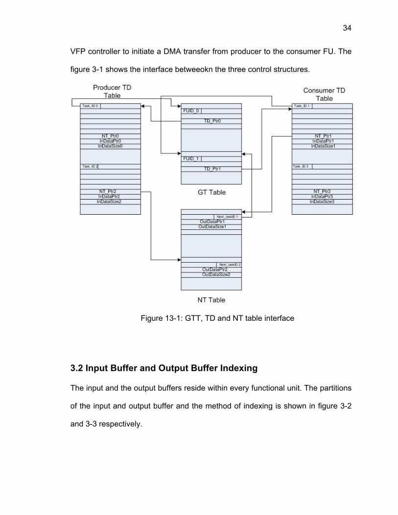
34
VFP controller to initiate a DMA transfer from producer to the consumer FU. The
figure 3-1 shows the interface betweeokn the three control structures.
Figure 13-1: GTT, TD and NT table interface
3.2 Input Buffer and Output Buffer Indexing
The input and the output buffers reside within every functional unit. The partitions
of the input and output buffer and the method of indexing is shown in figure 3-2
and 3-3 respectively.

35
3.2.1 Input Buffer
The input buffer is of size 64Kb, off which 32Kb is dedicated to the TD table. The
other half is partitioned into 16 buffers. The buffer 0 is of size 4Kb and contains
the data to be operated on by the PE. The buffer 1 contains the control
parameter information that is passed on by every FU and is of 64 bytes. The
remaining buffers can be programmed to be of variable sizes. The accessing of
the input buffer is as shown in the figure 3-2.
Figure 14: Input Buffer Partitions

36
3.2.2 Output Buffer
The output buffer is of size 64Kb and is accessed in a way similar to the input
buffer. The “out_data_ptr” for every region is specified in the register map local to
every PE. The PE accesses the register map to obtain the pointer information
and then writes into the address contained by the pointer. In case of flow context
the information is stored in the local register map.
Figure 15: Output Buffer Partitions

37
3.3 System Flow
The figure 3-4 depicts the system flow in detail. The sequence of operations is
also shown.
1. The VFP controller consists of dedicated Task Scheduler Queues (TSQ)
for every FU. The descriptor consists of the FUID, using which the
scheduler within the VFP controller schedules the task to the producer FU.
The descriptor formats are shown in the Appendix. The task can be
asynchronous, in which case it is scheduled immediately, or synchronous,
in which case it is scheduled once its start time occurs. The scheduler also
sets the “Busy Vector” field in the GTT that indicates that the particular FU
is busy in processing a task.
2. The Task Activation (TA) unit within the producer FU, accesses the TD
table whose pointer it received from the VFP controller. The TD table
contains all the relevant information required by the TA to trigger the PE,
such as the command number and flow context information. It also
updates the input buffer pointer and size information in the input buffer
that are required by the PE.
3. The PE reads the input data from the input buffer and operates on the
data.
4. The PE writes the result into the output buffer. On completing the task, the
PE sends out a “cmd_done” and a “next_task_en” signal.

38
5. The producer FU then sends out two messages, one corresponding to the
“cmd_done” to initiate the termination of task and the other corresponding
to “next_task_en” to trigger the next task – {5a, 5b}.
6. On receiving the command termination message, the Command
Termination (CT) block within the VFP, clears the Busy Vector in the GTT,
which marks the termination of the scheduled task. The producer FU is
now free to cater to other tasks. The “next_task_en” message sent by the
FU contains the physical address of the NT pointer. Using this address,
the Consumer Identification (CID) unit within the VFP, accesses the NT
table to identify the consumer FU’s. The producer FU also sends out the
physical address of the output buffer, where the processed data is stored.
It also sends out the size of the processed data. The output buffer address
serves as the source address during the data transfer over the bus, while
the “OutData_Ptr” field read from the NT table, serves as the destination
address. The CID sends out a message to the Data Transfer Initiator (DTI)
with the necessary source and destination address to activate the DMA
transfer.
7. The source and destination address and the size of the data transfer is
sent to the consumer FU identified by the VFP. The consumer FU now
initiates a transfer over the AXI bus.
8. The data is transferred by reading from the output buffer of the producer
FU and writing into the input buffer of the consumer FU.
9. Once the data transfer is completed, the consumer FU messages the VFP
controller. The Task Inserter (TI) unit within the VFP inserts a task into the

39
TSQ dedicated to the identified consumer FU. The local TI within the
consumer FU updates the TD table with the input buffer pointer and size
information.
Figure 16: System Flow
3.4 Task Scheduling
The two types of data tasks handled by the WiNC2R platform are asynchronous
and synchronous. Although, the actual processing engine is unaware of the type
of data task, the method of scheduling these tasks are different. The
“Sync/Async” field in the GTT determines the nature of the task; a value of 1
corresponds to asynchronous task while 0 corresponds to a synchronous task.
The synchronous task can be two kinds – chunking and non-chunking. The
chunking and non-chunking tasks are described in the later sections.
The asynchronous tasks are demand tasks, and hence are scheduled
immediately by the scheduler. In case the asynchronous task does not terminate

40
before the start time of a synchronous task, the asynchronous task can be
interrupted and is resumed after the completion of the synchronous task.
The synchronous tasks have pre-allocated time slots, and on the arrival of the
particular time, the synchronous task is scheduled. The synchronous task can
repeated based on the rescheduling period or the repetition number, both of
which are pre-defined in the GTT. The scheduler uses the rescheduling period to
repeat a particular synchronous task termed as a chunking task, while it uses the
repetition number to repeat the task incase of a non-chunking synchronous task.
3.4.1 Concept of Chunking
The input data can be broken up into smaller pieces called “chunks” of a pre-
defined size (chunksize) to improve the overall end-to-end latency of the system.
The “ChunkFlag” parameter in the GTT indicates whether the current task to be
scheduled is a chunking or non-chunking task. The current task is a chunking
task if the parameter is set. The functional unit handling the chunking task
obtains the chunksize and the first_chunksize information by reading the TD
table. It is the responsibility of the scheduler to keep a track of the number of
chunks. The “first_chunkflag” bit is set in the message sent by the scheduler to
the FU in case of first chunk and the “last_chunkflag” bit is set indicating that the
chunk is the final chunk. In case of the first chunk, the TA unit within the FU,
updates the size pointer in the input buffer with the first_chunksize and address
pointer with address obtained from the “InDataPtr” field in the TD table. The TA
unit then updates the “InDataPtr” field in the TD table with the previous
“InDataPtr” + first_chunksize and updates the “InDataSize” field in the TD by

41
deducting the first_chunksize from the total size. When the first_chunkflag bit is
not set, the TA updates the information the TD according to the chunksize. The
chunksize and the first_chunksize information are available in the GTT, which is
accessible by the scheduler. The scheduler deducts the chunksize or
first_chunksize (in case of first chunk only) from the total frame size and
schedules the next chunk only after a period called the “Reschduling Period”.
The last chunk is scheduled when the remaining frame size is lesser than the
chunksize and the last_chunkflag bit is set.
The following functional unit(s) can terminate the chunking or pass them along. If
the unit is passing along the chunks of data (i.e. it is neither chunking nor
terminating the chunking) the chunks will processed like the full frame – i.e. the
unit passing it along is not even aware of the chunking. If the unit it is terminating
the chunking for the particular task (TerminateChunking[x] == 1 in the Task
Descriptor) it will pass the results of each chunk processing to the following unit
as the chunks are being processed but it will enable the next task only when the
last chunk is processed. In this case the chunks are gathered into the frame at
the consumer task input buffer. Since the chunk termination unit needs to pass
the pointer to the beginning of the frame buffer to the consumer task it needs to
keep the OutDataPtr original value while the chunks are being processed and
passed along. For that purpose, in the de-chunking mode the output consumer
task entries (NextTaskIDx and associated pointers) are paired together so that
OutDataPtrx keeps the working pointer that gets incremented with the transfer of
each chunk by the corresponding OutDataSizex and OutDataPtr+1 that contains
the original OutDataPtr (before the transfer of the first chunk). The

42
OutDataSizex+1 is incremented after each chunk transfer by OutDataSizex, so
that it contains the whole frame after the last chunk has been transferred.
An optimum chunksize must be determined to achieve good system latency. The
following chapters discuss about the calculation of chunk size and its effect on
the latency of the system. The concept of chunking also helps in supporting
multiple flows (of different or same protocol) in the system. The analysis related
to multiple flows is also described in detail in the later chapters.

43
Chapter 4
WiNC2R Revision 2 Processing Engines
4.1: 802.11a Protocol Description
802.11a is an amendment to the IEEE 802.11 specification that added a
higher data rate of up to 54 Mbit/s using the 5 GHz band. It has seen widespread
worldwide implementation, particularly within the corporate workspace. The
802.11a standard uses the same core protocol as the original standard, operates
in 5 GHz band, and uses a 52-subcarrier orthogonal frequency-division
multiplexing (OFDM) with a maximum raw data rate of 54 Mbit/s, which yields
realistic net achievable throughput in the mid-20 Mbit/s. The data rate is reduced
to 48, 36, 24, 18, 12, 9 then 6 Mbit/s if required. The OFDM PHY contains three
functional entities: the physical medium dependent function, the PHY
convergence function, and the management function.(5)
• Physical Layer Convergence Procedure (PLCP) Sublayer:
In order to allow the IEEE 802.11 MAC to operate with minimum
dependence on the Physical Medium Dependent (PMD) sublayer, a PHY
convergence sublayer is defined. This function simplifies the PHY service
interface to the IEEE 802.11 MAC services. The PLCP sublayer is
described in detail in the following sections.

44
• Physical Medium Dependent (PMD) Sublayer:
The PMD sublayer provides a means to send and receive data between
two or more stations in the 5 GHz band using OFDM modulation.
• Physical Management Entity (PLME):
The PLME performs management of the local PHY functions in
conjunction with the MAC management entity.
4.1.1:PLCP Frame Format
(5)Figure 4-1 shows the format for the PLCP Protocol Data Unit (PPDU)
including the OFDM PLCP preamble, OFDM PLCP header, Physical layer
Service Data Unit (PSDU), tail bits, and pad bits. The PLCP header contains the
following fields: LENGTH, RATE, a reserved bit, an even parity bit, and the
SERVICE field. In terms of modulation, the LENGTH, RATE, reserved bit, and
parity bit (with 6 “zero” tail bits appended) constitute a separate single OFDM
symbol, denoted SIGNAL, which is transmitted with the most robust combination
of BPSK modulation and a coding rate of R = 1/2. The SERVICE field of the
PLCP header and the PSDU (with 6 “zero”tail bits and pad bits appended),
denoted as DATA, are transmitted at the data rate described in the RATE field
and may constitute multiple OFDM symbols. The tail bits in the SIGNAL symbol
enable decoding of the RATE and LENGTH fields immediately after the reception
of the tail bits. The RATE and LENGTH are required for decoding the DATA part
of the packet.

45
Figure 4-1: PPDU Frame Format
Source: IEEE 802.11a-1999, Wireless LAN MAC and PHY Specifications
The individual fields of the 802.11a PPDU frame are described below:
• PLCP Preamble: The PLCP preamble field is used for synchronization. It
consists of 10 short symbols and two long symbols as shown below in the
OFDM training sequence.
Figure 4-2: OFDM Training Sequence
Source: IEEE 802.11a-1999, Wireless LAN MAC and PHY Specifications
t1 – t10 denote the 10 short symbols, each symbol duration being 0.8us. T1 and T2
denote the 2 long symbols each of duration 3.2us. Thus, the total training
sequence sums up to 16us. The SIGNAL and the DATA fields follow the PLCP
preamble field.

46
• SIGNAL: The SIGNAL field is composed of 24 bits. Bits 0-3 encode the
RATE field, bit 4 is reserved for future use, bits 5-16 encode the LENGTH
field, bit 17 denotes the PARITY field and bits 18-23 denote the TAIL field.
o RATE: 802.11a protocol supports data rates ranging from 6
Mbits/sec to a maximum of 54Mbits/sec. The RATE field conveys
information about the coding rate to be used for the SIGNAL and
the PPDU. The encoding of the various rates is shown in the table
below:
RATE R0 – R3
6 1101
9 1111
12 0101
18 0111
24 1001
36 1011
48 0001
54 0011
Table 4-1: Rate Field Encoding
o Reserved: Bit 4 is reserved for future use.
o LENGTH: The PLCP length field is an unsigned 12-bit integer that
indicates the number of octets in the PSDU that the MAC is
currently requesting the PHY to transmit. This value is used by the
PHY to determine the number of octet transfers that will occur

47
between the MAC and the PHY after receiving a request to start
transmission.
o PARITY: Bit 17 denotes the parity bit. Even parity is selected for
bits 0 – 16.
o TAIL: Bits 18-23 constitute the TAIL field. All the 6 bits are set to
zero.
The SIGNAL field forms 1 OFDM symbol and is coded, interleaved,
modulated and converted to time domain. The SIGNAL field is NOT
scrambled and is BPSK modulated at a coding rate of ½ and transmitted
at 6Mbps.
• DATA: The DATA field of the 802.11a frame consists of PLCP header
SERVICE field, PSDU, 6 TAIL bits and PAD bits. Each field is described
below:
o SERVICE: SERVICE field has 16 bits, which shall be denoted as
bits 0 - 15. The bit 0 shall be transmitted first in time. The bits from
0 - 6 of the SERVICE field, which are transmitted first, are set to
zeros and are used to synchronize the descrambler in the receiver.
The remaining 9 bits (7 - 15) of the SERVICE field shall be
reserved for future use. All reserved bits shall be set to zero.
o PSDU: PSDU represents the contents of PPDU i.e. actual contents
of the 802.11a frame.
o TAIL: TAIL bit field shall be six bits of “0” which are required to
return the convolutional encoder to the “zero state”. This

48
procedure improves the error probability of the convolutional
decoder, which relies on future bits when decoding and which may
be not be available past the end of the message. The PLCP tail bit
field shall be produced by replacing six scrambled “zero” bits
following the message end with six nonscrambled “zero” bits.
o PAD: The number of bits in the DATA field of the PPDU frame is a
multiple of the number of coded bits (NCBPS) in an OFDM symbol.
To achieve that, the length of the message is extended so that it
becomes a multiple of NDBPS, the number of data bits per OFDM
symbol. At least 6 bits are appended to the message, in order to
accommodate the TAIL bits. The number of OFDM symbols, NSYM;
the number of bits in the DATA field, NDATA; and the number of pad
bits, NPAD, are computed from the length of the PSDU (LENGTH) as
follows:
NSYM = Ceiling ((16 + 8 * LENGTH + 6) / NDBPS
NDATA = NSYM * NDBPS
NPAD = NDATA – (16 + 8 * LENGTH + 6)

49
4.2: 802.11a TRANSMITTER
The processing units involved in an 802.11a transmitter are shown in the
Figure 4-3:
Figure 4-3: 802.11a Transmitter
Source: IEEE 802.11a-1999, Wireless LAN MAC and PHY Specifications
The 802.11a processing engines specifications are described in the sections that
follow. Since, WiNC2R Revision 1 implementation was a proof of concept, it did
not comprise of certain 802.11a processing engines such as scrambler, coder,
puncturer and interleaver. In revision2 we include all the processing blocks
involved in an 802.11a transmitter flow to achieve an ideal 802.11a transmission
flow.

50
4.3 WiNC2R 802.11a Transmitter Flow:
Figure 4-4: WiNC2R 802.11a Transmitter
The above figure depicts the WiNC2R transmitter flow. Some processing engines
such as PE_MAC, PE_HEADER(PE_HDR), PE_MODULATOR(PE_MOD) and
PE_IFFT are reused from the previous version of WiNC2R. The IFFT engine
performs the task of Preamble Generation, Cyclic Extension, IFFT and Pilot
Insertion. Engines such as scrambler, convolutional encoder and interleaver are
C functions which are imported from various sources, one being GNU Radio.
Thus, we have a combination of processing engines, some implemented in RTL
(VHDL/Verilog) and some C/C++ functions.
The following section gives a brief introduction of GNU Radio and the method
adopted to integrate the C / C++ functions into an RTL environment such as
WiNC2R.

51
4.3.1: GNU Radio
(6)The GNU Software Radio is an open source project that is hardware
independent to a certain extent. The free software kit consists of a library of
signal processing functions, which can be connected together to build and deploy
a software-defined radio (SDR). In order to implement an SDR, a signal graph
needs to be created which connects the source, signal processing blocks and the
sink together. The signal processing blocks, source and sink are C++ functions
and are connected together using a Python script.
4.3.2: Integrating GNU functions in WiNC2R
The revision2 of WiNC2R is a mixed HDL environment, where certain
blocks are coded in Verilog/SystemVerilog, while the blocks from revision 1 are in
VHDL. It was required to integrate the C++ GNU Radio functions into this mixed
HDL environment to implement an 802.11a transmission and reception. The C++
functions were integrated into the system using the concept of SystemVerilog
Direct Programming Interface (DPI).
4.3.3: Direct Programming Interface
(7)Direct Programming Interface (DPI) is an interface between
SystemVerilog and a foreign programming language. It consists of two separate
layers: the SystemVerilog layer and a foreign language layer. Both sides of DPI
are fully isolated. Which programming language is actually used as the foreign
language is transparent and irrelevant for the SystemVerilog side of this
interface. Neither the SystemVerilog compiler nor the foreign language compiler

52
is required to analyze the source code in the other’s language. Different
programming languages can be used and supported with the same intact
SystemVerilog layer. For now, however, SystemVerilog 3.1 defines a foreign
language layer only for the C programming language. DPI allows direct inter-
language function calls between the languages on either side of the interface.
Specifically, functions implemented in a foreign language can be called from
SystemVerilog; such functions are referred to as imported functions.
SystemVerilog functions that are to be called from a foreign code shall be
specified in export declarations.
4.3.4: Implementation
The desired processing block functions were taken from GNU radio and a
stand-alone C++ program was generated using the functions. The C++
processing functions were imported to a SystemVerilog wrapper file-using DPI.
The SV wrapper passes the arguments required for the C++ function to execute,
and the function returns back the final output to the SV wrapper. The SV module
can be port mapped with either the existing WiNC2R revision1 VHDL blocks or
revision2 Verilog/SystemVerilog modules. The figure below depicts the hierarchy
of WiNC2R revision2 implementation. The intermediate VHDL layer can be a
stand-alone processing engine from revision1 or can instantiate a SystemVerilog
wrapper that calls the C/ C++ function.

53
Figure 4-5: WiNC2R System Hierarchy
In this fashion the inputs required by the C++ function are passed from the top
level SystemVerilog file to middle layer of VHDL to the SystemVerilog wrapper
that calls that C++ function. In the similar manner, the outputs generated by C++
functions are passed to the top-level SystemVerilog file. In this way, it is possible
to integrate the GNU radio extracted C++ functions with the rest of WiNC2R.
4.3.5: Compiling
We required a simulator that had the capability to analyze, compile and
simulate mixed HDL designs descriptions. In addition to mixed HDL simulations,
it was also required that the simulator has the capability to handle imported
function calls from C++ or DPI. The VCS-MX simulator by Synopsys is a mixed
HDL simulator that catered to all our requirements.
System Verilog Top
VHDL
SystemVerilog Wrapper
C / C++ Functions
VHDL

54
4.4: WiNC2R Processing Engine Specifications
• PE_MAC_TX: This PE performs the tasks of a reconfigurable MAC and
currently supports two protocols – ALOHA and CSMA-CA back off. It also
uses 802.11a compatible inter-frame spacing (IFS) durations and fame
formats.
• PE_HEADER: This engine performs the task of appending the PLCP
header as shown in the PPDU frame format. It appends the header to the
frame sent by the PE_MAC_TX engine. This engine also instructs the
PE_IFFT to generate the PLCP preamble sequence by sending in a task
request to PE_IFFT engine. Apart from appending the PLCP header to the
frame, the PE_HEADER works on small parts of the frame termed as
“chunks”. The VFP controller dictates the size of each chunk and the
PE_HEADER operates on the specified size and treats each chunk as an
individual task. The successive processing engines now operate on
chunks and not the entire frame. The type of modulation scheme in use
and the data rate determine the size of individual chunk. In terms of
OFDM symbols, each chunk is equal to four OFDM symbols except the
last chunk. The PE_HEADER engine has two modes of operation – with
coder and no coder. The “with coder” mode implies that the frame is
encoded before modulation, while the “no coder” mode implies that no
encoding operation is being performed on the frame.

55
Chunk Size Calculation:
No Coder Case:
Chunk Size = (#OFDM symbols + Coded bits per OFDM symbol) / 8
With Coder Case:
Chunk Size = (#OFDM symbols + Data bits per OFDM symbol) / 8
The size of the first chunk is always different than the chunk size,
as the first chunk consists of the PLCP header and 16 service bits
in addition to the data.
FirstChunk = PLCP Header + 16 Service Bits + Data
PLCP Header = 1 OFDM symbol.
First Chunk Size = Chunk Size – (PLCP Header + 16 Service Bits)

56
Table 4-2 shows the computed values for chunksize and
firstchunksize for different data rates and modulation schemes.
Data Rate
(Mbps)
Modulation
Scheme
Coding
Rate
Coded bits
per OFDM
symbol
Data bits
per OFDM
symbol
FirstChunkSize
(bytes)
ChunkSize
(bytes)
6 BPSK ½ 48 24 7 12
9 BPSK ¾ 48 36 12 18
12 QPSK ½ 96 48 16 24
18 QPSK ¾ 96 72 25 36
24 16 – QAM ½ 192 96 34 48
36 16 – QAM ¾ 192 144 52 72
48 64 – QAM 2/3 288 192 70 96
54 64 – QAM 3/4 288` 216 79 108
Table 4-2: ChunkSize Calculation
The chunk size parameter dictates the performance of the WiNC2R architecture.
A smaller chunk size results in more number of chunks of the input frame, which
in turn leads to aggressive utilization of the VFP controller. Hence, there is a
direct relationship between chunk size and latency to transmit a frame belonging
to one flow. When the VFP controller handles multiple flows, each flow has a

57
different chunk size, which again affects the over-all system latency. The effect of
changing chunk size is discussed in detail in Chapter 5.
• PE_SCRAMBLER: Scrambler is a device that manipulates the data
stream before transmitting. A scrambler replaces sequences into other
sequences without removing undesirable sequences, and as a result it
changes the probability of occurrence of vexatious sequences. A
scrambler is implemented using memory elements (flip-flops) and modulo
2 adders (XOR gates). The connection between the memory elements
and modulo 2 adders is defined by the generator polynomial. Figure 4-6
below illustrates a scrambler. An appropriate descrambler is required at
the receiving end to recover back the original data.
Figure 4-6: Data Scrambler
Source: IEEE 802.11a-1999, Wireless LAN MAC and PHY Specifications
The PE_SCRAMBLER processing engine performs the task of
scrambling the DATA field of the PPDU frame format. The PLCP header
and the preamble bits of the PPDU frame are not scrambled. (5)The

58
scrambler is length-127 frame synchronous scrambler with a generator
polynomial
S(x) = x7 + x4 + 1 according to 802.11a protocol. A C++ scrambling
function from GNU Radio is integrated using SystemVerilog DPI into a
processing engine called PE_SCRAMBLER.
• PE_ENCODER: A convolutional code is a type of error correcting code in
which each “m” bit information symbol is transformed into an “n” bit symbol
where “m/n” is the code rate. A transformation function of “K” information
symbols is required, where “K” is the constraint length. An encoder
consists of “K” memory elements and “n” modulo 2 adders (XOR gates).
Figure 4-7 depicts a convolutional encoder of constraint length 7.
The DATA field, composed of SERVICE, PSDU, tail, and pad parts,
is encoded with a convolutional encoder of coding rate R = 1/2, 2/3, or 3/4,
corresponding to the desired data rate. (5)The convolutional encoder uses
the industry-standard generator polynomials, g0 = 1338 and g1 = 1718 for R
= ½. The bit denoted as “A” is the output from the encoder before the
bit denoted as “B”. Higher rates are derived from it by employing
“puncturing”. Puncturing is a procedure for omitting some of the encoded
bits in the transmitter (thus reducing the number of transmitted bits and
increasing the coding rate) and inserting a dummy “zero” metric into the
convolutional decoder on the receive side in place of the omitted bits.
Puncturer is not implemented in WiNC2R revision2.

59
A C function performing the task of convolutional encoder of rate ½
is integrated using SystemVerilog DPI into a processing engine called
PE_ENCODER. The engine supports only rate ½ encoding scheme.
Figure 4-7: Convolutional Encoder (Constraint Length 7)
Source: IEEE 802.11a-1999, Wireless LAN MAC and PHY Specifications
• PE_INTERLEAVER: Interleaving is method adopted in digital
communication systems to improve the performance of the forward error
correcting codes.
A C function of a block interleaver is integrated in the WiNC2R
system using SystemVerilog DPI. The C function implements a block
interleaver with block size equal to number of bits in a single OFDM
symbol. It performs a two-step process:
Permutation of bits in matrix by transposing it. The matrix is
16 column wide and “n” rows deep, where “n” varies
depending on the standard and code rate.

60
Carrying out logical and bit shift operations depending on the
standard and code rate.
• PE_MODULATOR: 802.11a protocol supports BPSK, QPSK, 16-QAM
and 64-QAM modulation schemes. We use the modulator that was
implemented in WiNC2R revision1, which is a VHDL entity supporting all
the above-mentioned modulation schemes. The PLCP header is always
BPSK rate ½ modulated, while the DATA field of the PPDU frame is
modulated depending on the data rate to be achieved, which is encoded in
the RATE field of the PLCP header.
• PE_IFFT: The PE_IFFT engine performs the task of pilot insertion for
each OFDM symbol, Inverse Fourier Transform (IFFT) of the data from the
modulator, cyclic prefix for each OFDM symbol and prefixing the preamble
bits at the beginning of the PPDU frame. The preamble generation is
triggered when the PE_IFFT engine receives a control task from
PE_HEADER. The PE_IFFT engine is a VHDL entity that was
implemented in WiNC2R revision 1.

61
CHAPTER 5
Performance Evaluation of WiNC2R
5.1 WiNC2R Test – Bench Using OVM
The verification platform used to validate WiNC2R revision2 architecture is based
on the concept of Open Verification Methodology (OVM) as against Xilinx Bus
Functional Module (BFM) used in revision1. The verification environment using
BFM was mainly used to load data into memories and did not serve the purpose
of validating the environment. On the other hand, by having a verification
environment based on OVM, one can load data into memories and also execute
random tests to validate the system architecture and hence have higher
confidence in the design. Figure 5-1 depicts the verification environment for
WiNC2R revision2 framework.

62
Figure 5-1: WiNC2R Verification Environment
As shown in the figure, the FU’s, VFP and OVM verification environment reside
within a cluster all connected to the main system bus The FU’s and VFP are
configured as master and slaves on the bus while the OVM verification
environment is configured as a master only. During initial system configuration,
the OVM loads the GTT, NTT and local TD tables. It also writes randomly
generated data into the FU_MAC_TX input buffer and triggers the system by
writing a descriptor into the FU_MAC_TX TSQ. On writing the descriptor, the
scheduler within the VFP gets triggered which later initiates the MAC_TX
processing engine.
The evaluation of the system is broadly divided into two sections:
• Effect of chunk size on the system latency
• Evaluation of multiple flow handling capability of the VFP

63
The following sections describe the experiments in detail and the results deduced
from each of the experiments. The basic experiment is described in detail that
gives an idea about the entire system flow.
5.1.1 Basic Experiment
The first experiment carried out to validate the system was to transmit a single
frame of size 64bytes at a rate of 6mbps. The frame is inserted into the
FU_MAC_TX engine and is propagated to the FU_IFFT engine. The figure 5-2
shows the command flow set up for the basic experiment. The
“Tx_Send_Data_Frame” task is inserted in the FU_MAC_TX and the successive
commands triggered are shown. The figure 5-3 depicts the transfer of the frame
starting from PE_MAC_TX and ending at PE_IFFT engine. The PE_IFFT engine
consists of FIFO from which the data is read at a constant rate and passed onto
the RF side for transmitting.
Figure 5-2: Single Flow Data Transfer
To avoid corruption of data before transmitting, it is necessary that the data being
read from the FIFO is continuous, i.e., the FIFO must never empty out or
overflow once reading has been initiated. The empty or overflow error conditions

64
are the ones that define the successful propagation of frame from PE_MAC_TX
to PE_IFFT engine.
Figure 5-3: WiNC2R Transmitter Frame Flow
The empty out or overflow condition at the PE_IFFT FIFO depends on the
latency of the system. The system latency is the difference between the times
when the FU_MAC_TX is triggered with the first command and the first data byte
appears at the output of FU_TX_IFFT. The system latency has a direct relation
with the Rescheduling Period parameter that is defined in the GTT for the task at
the PE_HDR and the processing time of each PE. The task at the FU_HDR is a
synchronous chunking task, i.e., the entire frame is broken up into smaller
number of chunks and each chunk is scheduled at a definite start time. The
Rescheduling Period parameter defines the difference between the start times of
2 chunks at the FU_HDR. The smaller the Rescheduling Period, the lesser is the
system latency as the chunks get scheduled quicker. On the other hand, with a
larger Rescheduling Period, the system latency increases as the chunks are
scheduled slower. Thus, overflow or empty out condition at the FU_IFFT FIFO

65
has a direct relation with the Rescheduling Period. If the FIFO empties out, it
implies that the chunks were scheduled too far apart. As a result the data chunks
did not reach the FU_IFFT in time and the FIFO was read out completely. This
causes data corruption and to avoid this scenario, we need to decrease the
Rescheduling Period. If the FIFO overflows, it means that the chunks were
scheduled too close to each other, and hence new data chunks are being written
in the FIFO, even before the existing chunks in the FIFO have been read out.
This cause corruption of data again and this scenario can be avoided by
increasing the Rescheduling Period.
The second parameter defining the latency of the system is processing time
required by each processing engine. The processing time determines the latency
introduced at every stage in the pipeline. Off the seven processing engines, we
have three processing engines that are C function based (scrambler, encoder
and interleaver) and hence their processing time can be varied. At present the
processing time for these engines have been set to a realistic number to build an
802.11a flow.
Pitfall: As shown in figure 4-2, the preamble generation task at the FU_IFFT is
triggered by the FU_HDR. Hence this task jumps the stages of the pipeline and is
activated. The FU_IFFT generates the preamble and stores it in the FIFO from
where it is read at a constant rate. To avoid data corruption, it is required that the
first data chunk is written into the FIFO before the preamble is completely read
out from the FIFO. From revision1 task flow, the preamble generation was an
asynchronous control task that gets scheduled immediately at the FU_IFFT with
the highest priority. In the new revision task flow, with addition of new processing

66
engines, the preamble generation task would get scheduled immediately and the
FIFO would empty out as there is an increase in latency of the data chunk. The
FIFO empty condition would occur even after reducing the rescheduling period
parameter to schedule the data chunks at FU_HDR faster. To overcome this
scenario, it was required to schedule the preamble generation task at the
FU_IFFT later in the pipeline stage. This was achieved by converting the
asynchronous control preamble generation task to a synchronous task. By
converting the task to a synchronous task, we have a greater control on
scheduling the task. The preamble task can now be triggered at a later stage in
the flow, thus ensuring that the FIFO empty error does not occur. The change
from asynchronous to synchronous task was easily achievable as it required only
changing the task type in the GTT. The error could have been overcome by
triggering the preamble generation at the FU_ENCODER or FU_INTERLEAVER
instead of the FU_HDR. This would have resulted in changing the PE’s to give
out the specific next task and status vector. On comparing the pros and cons of
the two solutions, it is seen that by changing the task to a synchronous task
would always give us more control on the start time of the preamble generation
task even in the future where there might be more processing engines in the
flow. This clearly brings out the flexibility in the WiNC2R system.
Throughput: The throughput of the system is defined as the number of data bits
transmitted per second. The revision2 WiNC2R supports rates of 6, 12 and 24
Mbps. We tested the throughput of our system for the mentioned rates only.
In an actual system, once the PE_IFFT writes the data into the FIFO, the data is
read by the DAC at a constant rate. Thus, by setting the reading rate of the FIFO

67
to an appropriate value we achieve the target throughput. The output of the IFFT
consists of complex symbols and hence the total size at the output of the IFFT is
greater than the input data size fed into the system. The formula to calculate the
required FIFO reading rate is shown below:
Information data (bits) / Rate = Complex data (bits) / FIFO Reading Rate
Thus,
FIFO Reading Rate = (Complex Data * Required Rate)/ Information Data
Once the reading rate of the FIFO is fixed to achieve the required throughput, the
Rescheduling Period must be altered in a way to avoid the FIFO from getting
empty. As we reduce the Rescheduling Period, the throughput increases. The
achieved throughput is calculated at the PE_HDR by measuring the time
required by the PE_HDR to process all the data chunks. The table 5-1 shows the
throughput achieved for different target rate requirements in a system supporting
a single flow. The throughput is calculated at the PE_HDR as explained. The
throughput calculated is the rate through the WiNC2R system before it is sent out
of the IFFT FIFO. If the throughput is measured at the FIFO, it will be at the
nominal rate.

68
Target Rate (Mbps) Peak Throughput
Measured at
HDR(Mbps)
6 7.47
12 16.25
24 34
Table 5-1: System Throughput
5.1.2 System Latency Experiment
This experiment deals with finding the latency of the system while supporting a
single flow of different rates. A total of 11 frames of size 400 bytes are sent
back – to – back for each rate.

69
Figure 5-4: Single Flow Latency
As noticed from the above graph, transmitting the first frame is always the best-
case scenario as all the processing engines are in their idle state and the
overhead introduced by the VFP controller is minimum. As more frames get lined
up in the pipeline, all the processing engines are busy at the same time and the
overhead introduced by the VFP controller also increases.
The system latency is a sum of three quantities.
1. Processing time of PE: This is the processing time taken by each PE to
process a single chunk of data.
2. DMA transfer time: This is time required to transfer a single data chunk
from FU_HDR to FU_IFFT.
0
1000
2000
3000
4000
5000
6000
7000
1 2 3 4 5 6 7 8 9 10 11
Latency (clk cycles)
Frame Number
Single Flow Latency
6mbps
12mbps
24mbps

70
3. VFP Processing Time: This is the time taken by the VFP controller to
schedule a task to the producer FU, identify the consumer FU and insert
the next task in the flow in the appropriate consumer FU.
5.1.3 Variation of chunk size on system latency
The chunk size described in section 3.4 plays an important role in defining the
latency of the system. As depicted in the Figure 4-2, the FU_MAC_TX transfers
the entire frame to the FU_HDR. The task executed by FU_HDR is a chunking
task, and hence FU_HDR works only on small chunks of the frame and passes
on the chunks to the successive FU’s. The final output is obtained at the
FU_IFFT. Thus, determining an optimum chunksize is necessary as it has a
direct effect on the latency of the system.
This experiment deals with varying the chunk size as shown in Table 3.2. We
send single frames of size 400 bytes at data rates of 6 and 12 Mbps. The chunk
size and the first chunk sizes are different for every rate and thus the aim of the
experiment is to see the effect of a larger chunk size on the system latency. The
chunksize and the first-chunksize calculated in Table 4.1 are under the
assumption that one chunk consists of four OFDM symbols. To vary the
chunksize, we have to vary the number of OFDM symbols in each chunk. The
Table 5-2 illustrates the variation in chunksize with different number of OFDM
symbols and the overall effect on system latency.

71
Rate
(Mbps)
OFDM
symbols
per chunk
Chunk
Size
(bytes)
First
Chunk
Size
(bytes)
Number of
chunks
Avg.Latency
(clk cycles)
6 4 12 7 34 3605
8 24 19 17 14099
12 4 24 16 17 4819
8 48 40 9 13437
24 4 48 34 9 5479
8 96 82 5 13450
Table 5-2: Variation of latency with chunksize
As the chunksize increases, the rescheduling period also increases. As a result,
the system latency increases even if the number of chunks is lesser. An optimum
number of OFDM symbols per chunk are required to support multiple flows. If the
number of OFDM symbols per chunk is less, lesser number of flows is supported,
as the rescheduling period is lesser. On the other hand, with greater number of
OFDM symbols per chunk, the system can support more multiple flows, but at
the expense of increased system latency.
5.1.4 Evaluation of Multiple Flow Support by VFP
An important feature of a cognitive radio is its ability to support multiple
technologies at the same time and also reusing the existing hardware. Hence,
the underlying hardware must be easily re-configurable to support different
72
technologies at the same time. The aim of this experiment is to see how
effectively the VFP switches between multiple flows. In the earlier revision of
WiNC2R, the VFP was local to every FU and hence would remain idle most of
the time after completing tasks allocated to the particular FU. To have a better
utilization of VFP, the VFP is centralized and hence it becomes important to see
the VFP utilization in case of multiple flows.
To support multiple flows, it is necessary that each flow have their own set of
tasks pre-defined. The tasks for every flow are populated in the GTT, NTT and
TD tables. The FU_TX_IFFT can handle a maximum of four OFDM flows. Each
flow is assigned a different channel id. On the basis of the channel id, the
FU_TX_IFFT engine is able to differentiate between flows, and stores the output
of each flow in a different FIFO, hence ensuring that the data from different flows
is not mixed with each other and corrupted. The number of channels imposes a
limitation on the system, as only a maximum of four flows can be supported at a
time. As the FU_MAC engine works on a single task a time, the earliest the next
flow can be inserted in the system is only after the FU_MAC completes operating
on the first flow.
Figure 5-4 depicts the command flow in case of a multiple flow scenario and
figure 5-5 shows the multiplexing of 2 flows.

73
Figure 5-5: Multiple Flow Data Transfer
Figure 5-6: Multiplexing of chunks in 2 flows
The experiment was carried out at rates 6, 12 and 24 Mbps for a frame size of
400 bytes and the effect of adding an extra flow on the latency and throughput of
the system was observed.
Limitation: As mentioned before, there are four FIFO’s available in FU_IFFT
which store the data to be sent to the DAC. Each FIFO is dedicated to a flow.

74
When the system is supporting multiple flows, it may happen that before a frame
is completely read out from the FIFO, the PE_IFFT engine gets the task of
generating the preamble for the succeeding frame of the same flow. In this case,
the preamble of the succeeding frame gets inserted into the FIFO even before
the preceding frame is completely read out leading to a channel error. To
overcome this scenario, we dedicate two FIFO’s to one flow. This way the first
frame is written into FIFO1 and the succeeding frame of the same flow gets
written into FIFO2. This pattern then gets repeated over multiple frames. As the
current implementation supports only four FIFO’s, we carried out the experiments
for two flows only.
The first experiment is to support to two flows of the same rate. The frame size
for both the flows is 400 bytes and frames are sent back-to-back in both flows.
The figures show the difference in the latency of a system supporting a single
flow versus two flows for rates 6 and 12 Mbps.

75
Figure 5-7: Variation in latency between single and two flows at rate
6Mbps
An increase in the latency of the system is noticed with the addition of one flow.
An increase of close to 88% is noticed in case of 12Mbps and 121% in case of
6Mbps. We suspect the increase in the latency is due to scheduling of the
available resources and are looking further into the different aspects that might
cause this problem.
0
2000
4000
6000
8000
10000
12000
1 2 3 4 5 6 7 8 9
Latency (clk cycles)
Frame Number
6mbps (Flow 1)
6mbps (Flow 2)
6mbps (Single Flow)

76
Figure 5-8: Variation in latency between single and two flows at rate 12Mbps
Figure 5-9: Variation in latency between single and two flows at rate 24Mbps
0
2000
4000
6000
8000
10000
12000
1 2 3 4 5 6 7 8 9 10 11
Latency (clk cycles)
Frame Number
12 mbps(Flow 1)
12 mbps (Flow 2)
12 mbps (single Flow)
0
2000
4000
6000
8000
10000
12000
1 2 3 4 5 6
Latency (clk cycles)
Frame Number
24Mbps(Single Flow)
24Mbps(Flow1)
24Mbps(Flow2)

77
It is necessary to increase the clock speed to meet the throughput requirement in
case multiple OFDM flows. The throughput achieved in case of running two flows
is shown at a higher clock rate is shown in table 5-2.
Target Rate (Mbps) Number of Flows Peak Throughput Measured
at HDR (Mbps)
6 2 26.98
12 2 51.06
24 2 88.5
Table 5-3: Throughput for two flows

78
CHAPTER 6
CONCLUSION AND FUTURE WORK
The WiNC2R was developed with an aim to achieve speed of operation through
hardware and re-configurability through software. From the analysis of the
system architecture, it is definitely proven that the WiNC2R platform is
reconfigurable to a great extent. In the new revision of WiNC2R, we have tried to
overcome the disadvantages of the previous revision, by having a new
centralized VFP controller catering to all the functional units. We replaced the
PLB bus with the AMBA AXI bus, which proves to be more efficient and helps in
reducing the bottleneck caused due to data transfer in the previous revision. We
have also set up a realistic transmitter having all the processing engines of the
802.11a protocol. The processing engines are now a mixture of hardware
engines and software engines having realistic latencies. This ensures that the
platform is able to support different types of processing engines depending on
the application.
The latency and throughput of the system was calculated for frames of rates of 6,
12 and 24 Mbps in a single flow. The system is able to support all the three rates.
We then analyzed the effect of changing the chunksize on the latency and
throughput. A higher throughput is achieved at a cost of higher latency by
increasing the chunksize. A chunksize of 4 OFDM symbols is considered
optimum to balance the tradeoff between latency and throughput.

79
An analysis was also done on the multiple flow support of the WiNC2R engine,
which is the core feature of any cognitive radio platform. The experiments were
run for flows supporting rates of 6, 12 and 24 mbps. A maximum of 2 flows is
supported by the current implementation. The system supports all the three rates
without any degradation in the throughput.
Future Work
The current architecture of the PE_IFFT engine imposes a limitation on the
latency and throughput of the system by ensuring that the FIFO’s don’t underflow
or overflow. This can be improved by terminating the chunks at the PE_IFFT
engine by the process of de-chunking. By de-chunking, the task at PE_IFFT will
be activated only once all the chunks have arrived. The PE_IFFT engine can also
generate the preamble on receiving the first chunk, hence removing the need to
trigger the task from FU_HDR.
As seen from the results, the latency increases drastically in case of multiple
flows as against a single flow. We need to analyze the overhead introduced by
the VFP controller to support multiple flows.

80
Bibliography [1]Resource Virtualization with Programmable Radio Processing Platform. Zoran
Miljanic, Predrag Spasojevic. 2008. WICON 2008.
[2] Satarkar, Sumit. PERFORMANCE ANALYSIS OF THE WINC2R PLATFORM.
Electrical and Computer Engineering, Rutgers, State University of New Jersey.
2009. Thesis.
[3] The winlab network centric cognitive radio hardware platform - WiNC2R.
Zoran Miljanic, Ivan Seskar, Khanh Le, and Dipankar Raychaudhuri. August
2007. Cognitive Radio Oriented Wireless Networks and Communications, 2007.
CrownCom 2007. 2nd International Conference. pp. 155 - 160.
[4] ARM. AMBA Open Specifications. [Online]
http://www.arm.com/products/system-ip/amba/amba-open-specifications.php.
[5] IEEE . IEEE 802.11a Physical and MAC Layer Specifications. 1999.
[6] Blossom, Eric. GNU Radio. [Online] www.gnuradio.org.
[7] Accellera. SystemVerilog 3.1a Language Reference Manual. [Online] 2004
http://www.vhdl.org/sv/SystemVerilog_3.1a.pdf.
[8] Cognitive radio: making software radios more personal. III Mitola, J. and Jr.
Maguire, G.Q. Aug 1999. Personal Communications, IEEE. pp. 13-18.
[9] Hari, Tejaswy. Physical Layer Design and Analysis of the WINLAB Network
Centric Cognitive Radio. Electrical and Computer Engineering, Rutgers, The
State University of New Jersey. 2009. Thesis.