system i performance capabilities reference version 6

System i Performance Capabilities Referencei5/OS™ Version 6, Release 1

January 2008

Thisdocument is intended for use by qualified performance related programmers or analysts fromIBM, IBM Business Partners and IBM customers using the System i platform. Information inthis document may be readily shared with IBM System i customers to understand theperformance and tuning factors in IBM i5/OS™ Version 6 Release 1. For the latest updatesand for the latest on System i performance information, please refer to the PerformanceManagement Website: http://www.ibm.com/systems/i/solutions/perfmgmt.

Requests for use of performance information by the technical trade press or consultants shouldbe directed to Systems Performance Department V3T, IBM Rochester Lab, in Rochester, MN.55901 USA.

V6R1 Performance Capabilities Reference - January 2008 © Copyright IBM Corp. 2008 System i Performance Capabilities 1

http://www.ibm.com/systems/i/solutions/perfmgmt

Note!

Before using this information, be sure to read the general information under “Special Notices.”

Twenty Fourth Edition (January 2008) SC41-0607-13

This edition applies to i5/OS Version 6, Release 1 of the System i platform.

You can request a copy of this document by download from i5/OS Information Center via the System i Internet site at: http://www.ibm.com/systems/i/ . The Version 5 Release 1 and Version 4 Release 5 Performance Capabilities Guides are alsoavailable on the IBM iSeries Internet site in the "On Line Library", at:http://publib.boulder.ibm.com/pubs/html/as400/online/chgfrm.htm.

Documents are viewable/downloadable in Adobe Acrobat (.pdf) format. Approximately 1 to 2 MB download. Adobe Acrobatreader plug-in is available at: http://www.adobe.com .

To request the CISC version (V3R2 and earlier), enter the following command on VM:

REQUEST V3R2 FROM FIELDSIT AT RCHVMW2 (your name)

To request the IBM iSeries Advanced 36 version, enter the following command on VM:

TOOLCAT MKTTOOLS GET AS4ADV36 PACKAGE

© Copyright International Business Machines Corporation 2008. All rights reserved.Note to U.S. Government Users -- Documentation related to restricted rights -- Use, duplication, or disclosure is subject torestrictions set forth in GSA ADP Schedule Contract with IBM Corp.


http://www.ibm.com/systems/i/

http://publib.boulder.ibm.com/pubs/html/as400/online/chgfrm.htm

http://www.adobe.com

Table of Contents

624.14 Performance References for DB2 . . . . . . . . . . . . . . . . . . . . . . . . . . . . . . . . . . . . . . . . . . . . . . . . .614.13 Reuse Deleted Record Space . . . . . . . . . . . . . . . . . . . . . . . . . . . . . . . . . . . . . . . . . . . . . . . . . . . . .594.12 Variable Length Fields . . . . . . . . . . . . . . . . . . . . . . . . . . . . . . . . . . . . . . . . . . . . . . . . . . . . . . . . . .584.11 Triggers . . . . . . . . . . . . . . . . . . . . . . . . . . . . . . . . . . . . . . . . . . . . . . . . . . . . . . . . . . . . . . . . . . . . .574.10 Referential Integrity . . . . . . . . . . . . . . . . . . . . . . . . . . . . . . . . . . . . . . . . . . . . . . . . . . . . . . . . . . . .564.9 DB2 Multisystem for i5/OS . . . . . . . . . . . . . . . . . . . . . . . . . . . . . . . . . . . . . . . . . . . . . . . . . . . . . . .534.8 Journaling and Commitment Control . . . . . . . . . . . . . . . . . . . . . . . . . . . . . . . . . . . . . . . . . . . . . . . .534.7 DB2 for i5/OS Memory Sharing Considerations . . . . . . . . . . . . . . . . . . . . . . . . . . . . . . . . . . . . . . .524.6 DB2 Symmetric Multiprocessing feature . . . . . . . . . . . . . . . . . . . . . . . . . . . . . . . . . . . . . . . . . . . . .514.5 Indexing . . . . . . . . . . . . . . . . . . . . . . . . . . . . . . . . . . . . . . . . . . . . . . . . . . . . . . . . . . . . . . . . . . . . . .494.4 V5R2 Highlights - Introduction of the SQL Query Engine . . . . . . . . . . . . . . . . . . . . . . . . . . . . . . .47Partitioned Table Support . . . . . . . . . . . . . . . . . . . . . . . . . . . . . . . . . . . . . . . . . . . . . . . . . . . . . . . .45i5/OS V5R3 SQE Query Coverage . . . . . . . . . . . . . . . . . . . . . . . . . . . . . . . . . . . . . . . . . . . . . . . . . .454.3 i5/OS V5R3 Highlights . . . . . . . . . . . . . . . . . . . . . . . . . . . . . . . . . . . . . . . . . . . . . . . . . . . . . . . . . . .44i5/OS V5R4 SQE Query Coverage . . . . . . . . . . . . . . . . . . . . . . . . . . . . . . . . . . . . . . . . . . . . . . . . . .444.2 DB2 i5/OS V5R4 Highlights . . . . . . . . . . . . . . . . . . . . . . . . . . . . . . . . . . . . . . . . . . . . . . . . . . . . . .41i5/OS V6R1 SQE Query Coverage . . . . . . . . . . . . . . . . . . . . . . . . . . . . . . . . . . . . . . . . . . . . . . . . . .414.1 New for i5/OS V6R1 . . . . . . . . . . . . . . . . . . . . . . . . . . . . . . . . . . . . . . . . . . . . . . . . . . . . . . . . . . . . .41Chapter 4. DB2 for i5/OS Performance . . . . . . . . . . . . . . . . . . . . . . . . . . . . . . . . . . . . . . . . . . . . . . .393.3 Tuning Parameters for Batch . . . . . . . . . . . . . . . . . . . . . . . . . . . . . . . . . . . . . . . . . . . . . . . . . . . . . .383.2 Effect of DASD Type on Batch . . . . . . . . . . . . . . . . . . . . . . . . . . . . . . . . . . . . . . . . . . . . . . . . . . . .383.1 Effect of CPU Speed on Batch . . . . . . . . . . . . . . . . . . . . . . . . . . . . . . . . . . . . . . . . . . . . . . . . . . . . .38Chapter 3. Batch Performance . . . . . . . . . . . . . . . . . . . . . . . . . . . . . . . . . . . . . . . . . . . . . . . . . . . . . .342.13.2 V5R1 DSD Performance Behavior . . . . . . . . . . . . . . . . . . . . . . . . . . . . . . . . . . . . . . . . . . . .342.13.1 V5R2 iSeries for Domino & DSD Performance Behavior updates . . . . . . . . . . . . . . . . . . . .342.13 iSeries for Domino and Dedicated Server for Domino Performance Behavior . . . . . . . . . . . . .332.12 Upgrade Considerations for Interactive Capacity . . . . . . . . . . . . . . . . . . . . . . . . . . . . . . . . . . . . .312.11 Migration from Traditional Models . . . . . . . . . . . . . . . . . . . . . . . . . . . . . . . . . . . . . . . . . . . . . . . .282.10 Managing Interactive Capacity . . . . . . . . . . . . . . . . . . . . . . . . . . . . . . . . . . . . . . . . . . . . . . . . . . .252.9 Server Dynamic Tuning (SDT) . . . . . . . . . . . . . . . . . . . . . . . . . . . . . . . . . . . . . . . . . . . . . . . . . . . .242.8 Interactive Utilization . . . . . . . . . . . . . . . . . . . . . . . . . . . . . . . . . . . . . . . . . . . . . . . . . . . . . . . . . . .232.7 Additional Server Considerations . . . . . . . . . . . . . . . . . . . . . . . . . . . . . . . . . . . . . . . . . . . . . . . . . .232.6 Performance Highlights of Custom Server Models . . . . . . . . . . . . . . . . . . . . . . . . . . . . . . . . . . . . .222.5 Performance Highlights of Model 170 Servers . . . . . . . . . . . . . . . . . . . . . . . . . . . . . . . . . . . . . . . .212.4 Performance Highlights of Model 7xx Servers . . . . . . . . . . . . . . . . . . . . . . . . . . . . . . . . . . . . . . . .192.3 Server Model Differences . . . . . . . . . . . . . . . . . . . . . . . . . . . . . . . . . . . . . . . . . . . . . . . . . . . . . . . .172.2.3 Existing Older Models . . . . . . . . . . . . . . . . . . . . . . . . . . . . . . . . . . . . . . . . . . . . . . . . . . . . . . .172.2.2 Choosing Between Similarly Rated Systems . . . . . . . . . . . . . . . . . . . . . . . . . . . . . . . . . . . . . .162.2.1 In V4R5 - V5R2 . . . . . . . . . . . . . . . . . . . . . . . . . . . . . . . . . . . . . . . . . . . . . . . . . . . . . . . . . . . .162.2 Server Model Behavior . . . . . . . . . . . . . . . . . . . . . . . . . . . . . . . . . . . . . . . . . . . . . . . . . . . . . . . . . .162.1.4 V5R2 and V5R1 . . . . . . . . . . . . . . . . . . . . . . . . . . . . . . . . . . . . . . . . . . . . . . . . . . . . . . . . . . .152.1.3 V5R3 . . . . . . . . . . . . . . . . . . . . . . . . . . . . . . . . . . . . . . . . . . . . . . . . . . . . . . . . . . . . . . . . . . . .152.1.2 Disclaimer and Remaining Sections . . . . . . . . . . . . . . . . . . . . . . . . . . . . . . . . . . . . . . . . . . . .142.1.1 Interactive Indicators and Metrics . . . . . . . . . . . . . . . . . . . . . . . . . . . . . . . . . . . . . . . . . . . . .142.1 Overview . . . . . . . . . . . . . . . . . . . . . . . . . . . . . . . . . . . . . . . . . . . . . . . . . . . . . . . . . . . . . . . . . . . . .14Chapter 2. iSeries and AS/400 RISC Server Model Performance Behavior . . . . . . . . . . . . . . . . .13Chapter 1. Introduction . . . . . . . . . . . . . . . . . . . . . . . . . . . . . . . . . . . . . . . . . . . . . . . . . . . . . . . . . . . .12Purpose of this Document . . . . . . . . . . . . . . . . . . . . . . . . . . . . . . . . . . . . . . . . . . . . . . . . . . . . . . . . . . .10Special Notices . . . . . . . . . . . . . . . . . . . . . . . . . . . . . . . . . . . . . . . . . . . . . . . . . . . . . . . . . . . . . . . . . . . .


15010.2 DB2 for i5/OS access with ODBC . . . . . . . . . . . . . . . . . . . . . . . . . . . . . . . . . . . . . . . . . . . . . . . .149References for JDBC . . . . . . . . . . . . . . . . . . . . . . . . . . . . . . . . . . . . . . . . . . . . . . . . . . . . . . . . . .148JDBC Performance Tuning Tips . . . . . . . . . . . . . . . . . . . . . . . . . . . . . . . . . . . . . . . . . . . . . . . . . .14810.1 DB2 for i5/OS access with JDBC . . . . . . . . . . . . . . . . . . . . . . . . . . . . . . . . . . . . . . . . . . . . . . . . .148Chapter 10. DB2 for i5/OS JDBC and ODBC Performance . . . . . . . . . . . . . . . . . . . . . . . . . . . . .1459.1 iSeries NetServer File Serving Performance . . . . . . . . . . . . . . . . . . . . . . . . . . . . . . . . . . . . . . . . .145Chapter 9. iSeries NetServer File Serving Performance . . . . . . . . . . . . . . . . . . . . . . . . . . . . . . . .1448.6 Additional Information . . . . . . . . . . . . . . . . . . . . . . . . . . . . . . . . . . . . . . . . . . . . . . . . . . . . . . . . .1438.5 Cryptography Observations, Tips and Recommendations . . . . . . . . . . . . . . . . . . . . . . . . . . . . . . .1418.4 Hardware Cryptographic API Performance . . . . . . . . . . . . . . . . . . . . . . . . . . . . . . . . . . . . . . . . . .1408.3 Software Cryptographic API Performance . . . . . . . . . . . . . . . . . . . . . . . . . . . . . . . . . . . . . . . . . .1398.2 Cryptography Performance Test Environment . . . . . . . . . . . . . . . . . . . . . . . . . . . . . . . . . . . . . . . .1388.1 System i Cryptographic Solutions . . . . . . . . . . . . . . . . . . . . . . . . . . . . . . . . . . . . . . . . . . . . . . . . . .138Chapter 8. Cryptography Performance . . . . . . . . . . . . . . . . . . . . . . . . . . . . . . . . . . . . . . . . . . . . . .137Resources . . . . . . . . . . . . . . . . . . . . . . . . . . . . . . . . . . . . . . . . . . . . . . . . . . . . . . . . . . . . . . . . . . . . . . .136Java i5/OS Database Access Tips . . . . . . . . . . . . . . . . . . . . . . . . . . . . . . . . . . . . . . . . . . . . . . . . .133Java Language Performance Tips . . . . . . . . . . . . . . . . . . . . . . . . . . . . . . . . . . . . . . . . . . . . . . . . .132Classic VM-specific Tips . . . . . . . . . . . . . . . . . . . . . . . . . . . . . . . . . . . . . . . . . . . . . . . . . . . . . . . .132i5/OS Specific Java Tips and Techniques . . . . . . . . . . . . . . . . . . . . . . . . . . . . . . . . . . . . . . . . . . . .131Introduction . . . . . . . . . . . . . . . . . . . . . . . . . . . . . . . . . . . . . . . . . . . . . . . . . . . . . . . . . . . . . . . . . .1317.7 Java Performance – Tips and Techniques . . . . . . . . . . . . . . . . . . . . . . . . . . . . . . . . . . . . . . . . . . .130General Guidelines . . . . . . . . . . . . . . . . . . . . . . . . . . . . . . . . . . . . . . . . . . . . . . . . . . . . . . . . . . . . .1307.6 Capacity Planning . . . . . . . . . . . . . . . . . . . . . . . . . . . . . . . . . . . . . . . . . . . . . . . . . . . . . . . . . . . . .1287.5 Determining Which JVM to Use . . . . . . . . . . . . . . . . . . . . . . . . . . . . . . . . . . . . . . . . . . . . . . . . . .127Bytecode Verification . . . . . . . . . . . . . . . . . . . . . . . . . . . . . . . . . . . . . . . . . . . . . . . . . . . . . . . . . . .126Garbage Collection . . . . . . . . . . . . . . . . . . . . . . . . . . . . . . . . . . . . . . . . . . . . . . . . . . . . . . . . . . . .124JIT Compiler . . . . . . . . . . . . . . . . . . . . . . . . . . . . . . . . . . . . . . . . . . . . . . . . . . . . . . . . . . . . . . . . . .1247.4 Classic VM (64-bit) . . . . . . . . . . . . . . . . . . . . . . . . . . . . . . . . . . . . . . . . . . . . . . . . . . . . . . . . . . . .123Garbage Collection . . . . . . . . . . . . . . . . . . . . . . . . . . . . . . . . . . . . . . . . . . . . . . . . . . . . . . . . . . . .123Native Code . . . . . . . . . . . . . . . . . . . . . . . . . . . . . . . . . . . . . . . . . . . . . . . . . . . . . . . . . . . . . . . . . .1227.3 IBM Technology for Java (32-bit and 64-bit) . . . . . . . . . . . . . . . . . . . . . . . . . . . . . . . . . . . . . . . . .1217.2 What’s new in V6R1 . . . . . . . . . . . . . . . . . . . . . . . . . . . . . . . . . . . . . . . . . . . . . . . . . . . . . . . . . . . .1217.1 Introduction . . . . . . . . . . . . . . . . . . . . . . . . . . . . . . . . . . . . . . . . . . . . . . . . . . . . . . . . . . . . . . . . . . .121Chapter 7. Java Performance . . . . . . . . . . . . . . . . . . . . . . . . . . . . . . . . . . . . . . . . . . . . . . . . . . . . . .1186.9 Connect for iSeries . . . . . . . . . . . . . . . . . . . . . . . . . . . . . . . . . . . . . . . . . . . . . . . . . . . . . . . . . . . .1186.8 WebSphere Commerce Payments . . . . . . . . . . . . . . . . . . . . . . . . . . . . . . . . . . . . . . . . . . . . . . . . .1176.7 WebSphere Commerce . . . . . . . . . . . . . . . . . . . . . . . . . . . . . . . . . . . . . . . . . . . . . . . . . . . . . . . . . .1176.6 WebSphere Portal . . . . . . . . . . . . . . . . . . . . . . . . . . . . . . . . . . . . . . . . . . . . . . . . . . . . . . . . . . . . . .1156.5 System Application Server Instance . . . . . . . . . . . . . . . . . . . . . . . . . . . . . . . . . . . . . . . . . . . . . . .1136.4 WebSphere Host Access Transformation Services (HATS) . . . . . . . . . . . . . . . . . . . . . . . . . . . . . .1036.3 IBM WebFacing . . . . . . . . . . . . . . . . . . . . . . . . . . . . . . . . . . . . . . . . . . . . . . . . . . . . . . . . . . . . . .

876.2 WebSphere Application Server . . . . . . . . . . . . . . . . . . . . . . . . . . . . . . . . . . . . . . . . . . . . . . . . . . . .786.1 HTTP Server (powered by Apache) . . . . . . . . . . . . . . . . . . . . . . . . . . . . . . . . . . . . . . . . . . . . . . . . .77Chapter 6. Web Server and WebSphere Performance . . . . . . . . . . . . . . . . . . . . . . . . . . . . . . . . . .765.9 Additional Information . . . . . . . . . . . . . . . . . . . . . . . . . . . . . . . . . . . . . . . . . . . . . . . . . . . . . . . . . . .755.8 HPR and Enterprise extender considerations . . . . . . . . . . . . . . . . . . . . . . . . . . . . . . . . . . . . . . . . . .735.7 APPC, ICF, CPI-C, and Anynet . . . . . . . . . . . . . . . . . . . . . . . . . . . . . . . . . . . . . . . . . . . . . . . . . . . .715.6 Performance Observations and Tips . . . . . . . . . . . . . . . . . . . . . . . . . . . . . . . . . . . . . . . . . . . . . . . . .685.5 TCP/IP Secure Performance . . . . . . . . . . . . . . . . . . . . . . . . . . . . . . . . . . . . . . . . . . . . . . . . . . . . . . .655.2 Communication Performance Test Environment . . . . . . . . . . . . . . . . . . . . . . . . . . . . . . . . . . . . . . .63Chapter 5. Communications Performance . . . . . . . . . . . . . . . . . . . . . . . . . . . . . . . . . . . . . . . . . . . . .


19014.1.3.1 571B RAID-5 vs RAID-6 - 10 15K 35GB DASD . . . . . . . . . . . . . . . . . . . . . . . . . . . . . . .19014.1.3 571B . . . . . . . . . . . . . . . . . . . . . . . . . . . . . . . . . . . . . . . . . . . . . . . . . . . . . . . . . . . . . . . . .18814.1.2 V5R2 Direct Attach DASD . . . . . . . . . . . . . . . . . . . . . . . . . . . . . . . . . . . . . . . . . . . . . . . . . . . .18714.1.1 Hardware Characteristics . . . . . . . . . . . . . . . . . . . . . . . . . . . . . . . . . . . . . . . . . . . . . . .18714.1.0 Direct Attach (Native) . . . . . . . . . . . . . . . . . . . . . . . . . . . . . . . . . . . . . . . . . . . . . . . . . . . . . . . .18614.1 Internal (Native) Attachment. . . . . . . . . . . . . . . . . . . . . . . . . . . . . . . . . . . . . . . . . . . . . . . . . . . .186Chapter 14. DASD Performance . . . . . . . . . . . . . . . . . . . . . . . . . . . . . . . . . . . . . . . . . . . . . . . . . . .18213.9 Top Tips for Linux on iSeries Performance . . . . . . . . . . . . . . . . . . . . . . . . . . . . . . . . . . . . . . . . .18213.8 Linux on iSeries and IBM eServer Workload Estimator . . . . . . . . . . . . . . . . . . . . . . . . . . . . . . .18113.7 DB2 UDB for Linux on iSeries . . . . . . . . . . . . . . . . . . . . . . . . . . . . . . . . . . . . . . . . . . . . . . . . . . .180Virtual Disk . . . . . . . . . . . . . . . . . . . . . . . . . . . . . . . . . . . . . . . . . . . . . . . . . . . . . . . . . . . . . . . . . .180Virtual LAN . . . . . . . . . . . . . . . . . . . . . . . . . . . . . . . . . . . . . . . . . . . . . . . . . . . . . . . . . . . . . . . . . .18013.6 Value of Virtual LAN and Virtual Disk . . . . . . . . . . . . . . . . . . . . . . . . . . . . . . . . . . . . . . . . . . . .180The Gcc Compiler, Version 3 . . . . . . . . . . . . . . . . . . . . . . . . . . . . . . . . . . . . . . . . . . . . . . . . . . . . .179Gcc and High Optimization (gcc compiler option -O3) . . . . . . . . . . . . . . . . . . . . . . . . . . . . . . . . .179Network Operations . . . . . . . . . . . . . . . . . . . . . . . . . . . . . . . . . . . . . . . . . . . . . . . . . . . . . . . . . . . .178Web Serving Performance . . . . . . . . . . . . . . . . . . . . . . . . . . . . . . . . . . . . . . . . . . . . . . . . . . . . . . .178Computational Performance -- Java . . . . . . . . . . . . . . . . . . . . . . . . . . . . . . . . . . . . . . . . . . . . . . .177Computational Performance -- C-based code . . . . . . . . . . . . . . . . . . . . . . . . . . . . . . . . . . . . . . . .17713.5 General Performance Information and Results . . . . . . . . . . . . . . . . . . . . . . . . . . . . . . . . . . . . . . .17613.4 Basic Configuration and Performance Questions . . . . . . . . . . . . . . . . . . . . . . . . . . . . . . . . . . . . .175Linux on iSeries Run-time Support . . . . . . . . . . . . . . . . . . . . . . . . . . . . . . . . . . . . . . . . . . . . . . . . .174Linux on iSeries Architecture . . . . . . . . . . . . . . . . . . . . . . . . . . . . . . . . . . . . . . . . . . . . . . . . . . . . .17413.3 Linux on iSeries Technical Overview . . . . . . . . . . . . . . . . . . . . . . . . . . . . . . . . . . . . . . . . . . . . . .17313.2 Basic Requirements -- Where Linux Runs . . . . . . . . . . . . . . . . . . . . . . . . . . . . . . . . . . . . . . . . . .173Key Ideas . . . . . . . . . . . . . . . . . . . . . . . . . . . . . . . . . . . . . . . . . . . . . . . . . . . . . . . . . . . . . . . . . . . .17313.1 Summary . . . . . . . . . . . . . . . . . . . . . . . . . . . . . . . . . . . . . . . . . . . . . . . . . . . . . . . . . . . . . . . . . . . .173Chapter 13. Linux on iSeries Performance . . . . . . . . . . . . . . . . . . . . . . . . . . . . . . . . . . . . . . . . . . .17112.4 Conclusions, Recommendations and Tips . . . . . . . . . . . . . . . . . . . . . . . . . . . . . . . . . . . . . . . . . .17112.3 Test Description and Results . . . . . . . . . . . . . . . . . . . . . . . . . . . . . . . . . . . . . . . . . . . . . . . . . . . .17012.2 Performance Improvements for WebSphere MQ V5.3 CSD6 . . . . . . . . . . . . . . . . . . . . . . . . . . .17012.1 Introduction . . . . . . . . . . . . . . . . . . . . . . . . . . . . . . . . . . . . . . . . . . . . . . . . . . . . . . . . . . . . . . . . .170Chapter 12. WebSphere MQ for iSeries . . . . . . . . . . . . . . . . . . . . . . . . . . . . . . . . . . . . . . . . . . . . .16911.14 System i NotesBench Audits and Benchmarks . . . . . . . . . . . . . . . . . . . . . . . . . . . . . . . . . . . . . .16811.13 LPAR and Partial Processor Considerations . . . . . . . . . . . . . . . . . . . . . . . . . . . . . . . . . . . . . . .16711.12 Sizing Domino on System i . . . . . . . . . . . . . . . . . . . . . . . . . . . . . . . . . . . . . . . . . . . . . . . . . . .16411.11 Main Storage Options . . . . . . . . . . . . . . . . . . . . . . . . . . . . . . . . . . . . . . . . . . . . . . . . . . . . . . . .16311.10 Performance Monitoring Statistics . . . . . . . . . . . . . . . . . . . . . . . . . . . . . . . . . . . . . . . . . . . . . . .16311.9 Domino Subsystem Tuning . . . . . . . . . . . . . . . . . . . . . . . . . . . . . . . . . . . . . . . . . . . . . . . . . . . . .16211.8 Domino Web Access . . . . . . . . . . . . . . . . . . . . . . . . . . . . . . . . . . . . . . . . . . . . . . . . . . . . . . . . . .15911.7 Performance Tips / Techniques . . . . . . . . . . . . . . . . . . . . . . . . . . . . . . . . . . . . . . . . . . . . . . . . . .15911.6 Collaboration Edition and Domino Edition offerings . . . . . . . . . . . . . . . . . . . . . . . . . . . . . . . . .15811.5 Response Time and Megahertz relationship . . . . . . . . . . . . . . . . . . . . . . . . . . . . . . . . . . . . . . .157Domino Web Access client improvements with Domino 6 . . . . . . . . . . . . . . . . . . . . . . . . . . . . . . .156Notes client improvements with Domino 6 . . . . . . . . . . . . . . . . . . . . . . . . . . . . . . . . . . . . . . . . . . .15611.4 Domino 6 . . . . . . . . . . . . . . . . . . . . . . . . . . . . . . . . . . . . . . . . . . . . . . . . . . . . . . . . . . . . . . . . . . .15511.3 Domino 7 . . . . . . . . . . . . . . . . . . . . . . . . . . . . . . . . . . . . . . . . . . . . . . . . . . . . . . . . . . . . . . . . . . .15511.2 Domino 8 . . . . . . . . . . . . . . . . . . . . . . . . . . . . . . . . . . . . . . . . . . . . . . . . . . . . . . . . . . . . . . . . . . .15411.1 Domino Workload Descriptions . . . . . . . . . . . . . . . . . . . . . . . . . . . . . . . . . . . . . . . . . . . . . . . . .153Chapter 11. Domino on System i . . . . . . . . . . . . . . . . . . . . . . . . . . . . . . . . . . . . . . . . . . . . . . . . . . .152References for ODBC . . . . . . . . . . . . . . . . . . . . . . . . . . . . . . . . . . . . . . . . . . . . . . . . . . . . . . . . . . .


23715.16 Save and Restore Scaling using 571E IOAs and U320 15K DASD units to a3580 Ultrium 3 Tape Drive. . . . . . . . . . . . . . . . . . . . . . . . . . . . . . . . . . . . . . . . . . . . . . . . . . . . . . . . . .

23615.15 Save and Restore Scaling using a Virtual Tape Drive. . . . . . . . . . . . . . . . . . . . . . . . . . . . . . . . .23515.14 Concurrent Virtual Tapes . . . . . . . . . . . . . . . . . . . . . . . . . . . . . . . . . . . . . . . . . . . . . . . . . . . . . .23415.13 Parallel Virtual Tapes . . . . . . . . . . . . . . . . . . . . . . . . . . . . . . . . . . . . . . . . . . . . . . . . . . . . . . . . .23215.12 Virtual Tape . . . . . . . . . . . . . . . . . . . . . . . . . . . . . . . . . . . . . . . . . . . . . . . . . . . . . . . . . . . . . . . .23115.11 DASD and Backup Devices Sharing a Tower . . . . . . . . . . . . . . . . . . . . . . . . . . . . . . . . . . . . . .23015.10 Number of Processors Affect Performance . . . . . . . . . . . . . . . . . . . . . . . . . . . . . . . . . . . . . . . .22915.9.4 User Mix Concurrent . . . . . . . . . . . . . . . . . . . . . . . . . . . . . . . . . . . . . . . . . . . . . . . . . . . . .22815.9.3 Large File Parallel . . . . . . . . . . . . . . . . . . . . . . . . . . . . . . . . . . . . . . . . . . . . . . . . . . . . . . .22715.9.2 Large File Concurrent . . . . . . . . . . . . . . . . . . . . . . . . . . . . . . . . . . . . . . . . . . . . . . . . . . . .22615.9.1 Hardware (2757 IOAs, 2844 IOPs, 15K RPM DASD) . . . . . . . . . . . . . . . . . . . . . . . . . . .22615.9 Parallel and Concurrent Library Measurements . . . . . . . . . . . . . . . . . . . . . . . . . . . . . . . . . . . . .22515.8 The Use of Multiple Backup Devices . . . . . . . . . . . . . . . . . . . . . . . . . . . . . . . . . . . . . . . . . . . . .22415.7 Ultra High Performing Backup Devices . . . . . . . . . . . . . . . . . . . . . . . . . . . . . . . . . . . . . . . . . . .22415.6 Medium & High Performing Backup Devices . . . . . . . . . . . . . . . . . . . . . . . . . . . . . . . . . . . . . .22415.5 Lower Performing Backup Devices . . . . . . . . . . . . . . . . . . . . . . . . . . . . . . . . . . . . . . . . . . . . . . .22315.4 Comparing Performance Data . . . . . . . . . . . . . . . . . . . . . . . . . . . . . . . . . . . . . . . . . . . . . . . . . . .22215.3 Workloads . . . . . . . . . . . . . . . . . . . . . . . . . . . . . . . . . . . . . . . . . . . . . . . . . . . . . . . . . . . . . . . . . .221Data Compaction (COMPACT) . . . . . . . . . . . . . . . . . . . . . . . . . . . . . . . . . . . . . . . . . . . . . . . . . . .221Data Compression (DTACPR) . . . . . . . . . . . . . . . . . . . . . . . . . . . . . . . . . . . . . . . . . . . . . . . . . . . .221Use Optimum Block Size (USEOPTBLK) . . . . . . . . . . . . . . . . . . . . . . . . . . . . . . . . . . . . . . . . . . . .22115.2 Save Command Parameters that Affect Performance . . . . . . . . . . . . . . . . . . . . . . . . . . . . . . . . .22015.1 Supported Backup Device Rates . . . . . . . . . . . . . . . . . . . . . . . . . . . . . . . . . . . . . . . . . . . . . . . . .220Chapter 15. Save/Restore Performance . . . . . . . . . . . . . . . . . . . . . . . . . . . . . . . . . . . . . . . . . . . . . .21914.5.1.3.2 Configuration Considerations . . . . . . . . . . . . . . . . . . . . . . . . . . . . . . . . . . . . . . . . . . .21414.5.1.3.1 7998-61X Blade running i5/OS/VIOS Performance . . . . . . . . . . . . . . . . . . . . . . . . .21414.5.1.3 VIOS and Blades Considerations . . . . . . . . . . . . . . . . . . . . . . . . . . . . . . . . . . . . . . . . . . . . . .212

14.5.1.3 Specific VIOS Configuration Recommendations -- Traditional (non-blade)Machines . . . . . . . . . . . . . . . . . . . . . . . . . . . . . . . . . . . . . . . . . . . . . . . . . . . . . . . . . . . . . . . . . . . . . . . .

20914.5.1.2 Generic Configuration Concepts . . . . . . . . . . . . . . . . . . . . . . . . . . . . . . . . . . . . . . . . . . . . . .20814.5.1.1 Generic Concepts . . . . . . . . . . . . . . . . . . . . . . . . . . . . . . . . . . . . . . . . . . . . . . . . . . . . . . .20814.5.1 General VIOS Considerations . . . . . . . . . . . . . . . . . . . . . . . . . . . . . . . . . . . . . . . . . . . . . . . . . .20614.4 SAN - Storage Area Network (External) . . . . . . . . . . . . . . . . . . . . . . . . . . . . . . . . . . . . . . . . . . .20414.3.1 Encrypted ASP . . . . . . . . . . . . . . . . . . . . . . . . . . . . . . . . . . . . . . . . . . . . . . . . . . . . . . . . . . .20414.3 New in V6R1M0 . . . . . . . . . . . . . . . . . . . . . . . . . . . . . . . . . . . . . . . . . . . . . . . . . . . . . . . . . . . . . .20314.2.3 12X Loop Testing . . . . . . . . . . . . . . . . . . . . . . . . . . . . . . . . . . . . . . . . . . . . . . . . . . . . . . . . .20214.2.2 RAID Hot Spare . . . . . . . . . . . . . . . . . . . . . . . . . . . . . . . . . . . . . . . . . . . . . . . . . . . . . . . . . .20114.2.1 9406-MMA CEC vs 9406-570 CEC DASD . . . . . . . . . . . . . . . . . . . . . . . . . . . . . . . . . . . .20114.2 New in V5R4M5 . . . . . . . . . . . . . . . . . . . . . . . . . . . . . . . . . . . . . . . . . . . . . . . . . . . . . . . . . . . . . .20014.1.10 Direct Attach 571E/574F and 571F/575B Observations . . . . . . . . . . . . . . . . . . . . . . . . .19814.1.9 Investigating 571E/574F and 571F/575B IOA, Bus and HSL limitations. . . . . . . . . . . . .19714.1.8 Performance Limits on the 571F/575B . . . . . . . . . . . . . . . . . . . . . . . . . . . . . . . . . . . . . . .19514.1.7 Comparing 571E/574F and 571F/575B RAID-5 and RAID-6 and Mirroring . . . . . . . . . .19414.1.6 Comparing 571E/574F and 571F/575B IOP and IOPLess . . . . . . . . . . . . . . . . . . . . . . . . .193

14.1.5 Comparing Current 2780/574F with the new 571E/574F and 571F/575BNOTE: V5R3 has support for the features in this section but all of ourperformance measurements were done on V5R4 systems. For information on thesupported features see the IBM Product Announcement Letters. . . . . . . . . . . . . . . . . . . . . . . . . . .

19114.1.4 571B, 5709, 573D, 5703, 2780 IOA Comparison Chart . . . . . . . . . . . . . . . . . . . . . . . . . .19014.1.3.2 571B IOP vs IOPLESS - 10 15K 35GB DASD . . . . . . . . . . . . . . . . . . . . . . . . . . . . . . . . .


272General Tips . . . . . . . . . . . . . . . . . . . . . . . . . . . . . . . . . . . . . . . . . . . . . . . . . . . . . . . . . . . . . . . . . .272V5R2 Additions . . . . . . . . . . . . . . . . . . . . . . . . . . . . . . . . . . . . . . . . . . . . . . . . . . . . . . . . . . . . . . . .272V5R3 Information . . . . . . . . . . . . . . . . . . . . . . . . . . . . . . . . . . . . . . . . . . . . . . . . . . . . . . . . . . . . . .27218.1 Introduction . . . . . . . . . . . . . . . . . . . . . . . . . . . . . . . . . . . . . . . . . . . . . . . . . . . . . . . . . . . . . . . . . .272Chapter 18. Logical Partitioning (LPAR) . . . . . . . . . . . . . . . . . . . . . . . . . . . . . . . . . . . . . . . . . . . .27017.9 Additional Sources of Information . . . . . . . . . . . . . . . . . . . . . . . . . . . . . . . . . . . . . . . . . . . . . . . .27017.8 Summary . . . . . . . . . . . . . . . . . . . . . . . . . . . . . . . . . . . . . . . . . . . . . . . . . . . . . . . . . . . . . . . . . . . .26917.7 File Level Backup Performance . . . . . . . . . . . . . . . . . . . . . . . . . . . . . . . . . . . . . . . . . . . . . . . . . .26817.6.3 Windows CPU Cost . . . . . . . . . . . . . . . . . . . . . . . . . . . . . . . . . . . . . . . . . . . . . . . . . . . . . . .26817.6.2 VE CPW Cost . . . . . . . . . . . . . . . . . . . . . . . . . . . . . . . . . . . . . . . . . . . . . . . . . . . . . . . . . . .26717.6.1 VE Capacity Comparisons . . . . . . . . . . . . . . . . . . . . . . . . . . . . . . . . . . . . . . . . . . . . . . . . .26617.6 Virtual Ethernet CPU Cost and Capacities . . . . . . . . . . . . . . . . . . . . . . . . . . . . . . . . . . . . . . . . . .26517.5 Disk I/O Throughput . . . . . . . . . . . . . . . . . . . . . . . . . . . . . . . . . . . . . . . . . . . . . . . . . . . . . . . . . . .26417.4.1 Further notes about IXS/IXA Disk Operations . . . . . . . . . . . . . . . . . . . . . . . . . . . . . . . . . .26317.4 Disk I/O CPU Cost . . . . . . . . . . . . . . . . . . . . . . . . . . . . . . . . . . . . . . . . . . . . . . . . . . . . . . . . . . . .26217.3.2 iSCSI attached servers: . . . . . . . . . . . . . . . . . . . . . . . . . . . . . . . . . . . . . . . . . . . . . . . . . . . .26217.3.1 IXS and IXA attached servers: . . . . . . . . . . . . . . . . . . . . . . . . . . . . . . . . . . . . . . . . . . . . . . .26217.3 System i memory rules of thumb for IXS/IXA and iSCSI attached servers. . . . . . . . . . . . . . . . .26217.2.5 IXS/IXA IOP Resource: . . . . . . . . . . . . . . . . . . . . . . . . . . . . . . . . . . . . . . . . . . . . . . . . . . .26117.2.4 Virtual Ethernet Connections: . . . . . . . . . . . . . . . . . . . . . . . . . . . . . . . . . . . . . . . . . . . . . .26017.2.3 iSCSI virtual I/O private memory pool . . . . . . . . . . . . . . . . . . . . . . . . . . . . . . . . . . . . . . . .25917.2.2 iSCSI Disk I/O Operations: . . . . . . . . . . . . . . . . . . . . . . . . . . . . . . . . . . . . . . . . . . . . . . . . .25817.2.1 IXS/IXA Disk I/O Operations: . . . . . . . . . . . . . . . . . . . . . . . . . . . . . . . . . . . . . . . . . . . . . . .25817.2 Effects of Windows and Linux loads on the host system . . . . . . . . . . . . . . . . . . . . . . . . . . . . . . .25717.1 Introduction . . . . . . . . . . . . . . . . . . . . . . . . . . . . . . . . . . . . . . . . . . . . . . . . . . . . . . . . . . . . . . . . . .257Chapter 17. Integrated BladeCenter and System x Performance . . . . . . . . . . . . . . . . . . . . . . . . .25616.11 IPL Tips . . . . . . . . . . . . . . . . . . . . . . . . . . . . . . . . . . . . . . . . . . . . . . . . . . . . . . . . . . . . . . . . . . .25616.10 5XX IOP vs IOPLess effects on IPL Performance (Normal) . . . . . . . . . . . . . . . . . . . . . . . . . . .25516.9 5XX IPL Performance Measurements (Abnormal) . . . . . . . . . . . . . . . . . . . . . . . . . . . . . . . . . . . .25516.8 5XX IPL Performance Measurements (Normal) . . . . . . . . . . . . . . . . . . . . . . . . . . . . . . . . . . . . . .25416.7.2 5XX Large system Hardware Configuration . . . . . . . . . . . . . . . . . . . . . . . . . . . . . . . . . . . .25416.7.1 5XX Small system Hardware Configuration . . . . . . . . . . . . . . . . . . . . . . . . . . . . . . . . . . . .25416.7 5XX System Hardware Information . . . . . . . . . . . . . . . . . . . . . . . . . . . . . . . . . . . . . . . . . . . . . . .25316.6.1 MSD Affects on IPL Performance Measurements . . . . . . . . . . . . . . . . . . . . . . . . . . . . . . . .25316.6 NOTES on MSD . . . . . . . . . . . . . . . . . . . . . . . . . . . . . . . . . . . . . . . . . . . . . . . . . . . . . . . . . . . . . .25216.5 9406-MMA IPL Performance Measurements (Abnormal) . . . . . . . . . . . . . . . . . . . . . . . . . . . . . .25216.4 9406-MMA IPL Performance Measurements (Normal) . . . . . . . . . . . . . . . . . . . . . . . . . . . . . . .25116.3.2 Large system Hardware Configurations . . . . . . . . . . . . . . . . . . . . . . . . . . . . . . . . . . . . . .25116.3.1 Small system Hardware Configuration . . . . . . . . . . . . . . . . . . . . . . . . . . . . . . . . . . . . . . .25116.3 9406-MMA System Hardware Information . . . . . . . . . . . . . . . . . . . . . . . . . . . . . . . . . . . . . . . . .25016.2 IPL Test Description . . . . . . . . . . . . . . . . . . . . . . . . . . . . . . . . . . . . . . . . . . . . . . . . . . . . . . . . . . .25016.1 IPL Performance Considerations . . . . . . . . . . . . . . . . . . . . . . . . . . . . . . . . . . . . . . . . . . . . . . . . .250Chapter 16 IPL Performance . . . . . . . . . . . . . . . . . . . . . . . . . . . . . . . . . . . . . . . . . . . . . . . . . . . . . .24815.24 9406-MMA 576B IOPLess IOA . . . . . . . . . . . . . . . . . . . . . . . . . . . . . . . . . . . . . . . . . . . . . .24715.23 9406-MMA DVD RAM . . . . . . . . . . . . . . . . . . . . . . . . . . . . . . . . . . . . . . . . . . . . . . . . . . . . .24515.21 5XX DVD RAM and Optical Library . . . . . . . . . . . . . . . . . . . . . . . . . . . . . . . . . . . . . . . . . . . .244

15.20 5XX Tape Device Rates with 571E & 571F Storage IOAs and 4327 (U320)Disk Units . . . . . . . . . . . . . . . . . . . . . . . . . . . . . . . . . . . . . . . . . . . . . . . . . . . . . . . . . . . . . . . . . . . . . . .

24015.18 BRMS-Based Save/Restore Software Encryption and DASD-Based ASPEncryption . . . . . . . . . . . . . . . . . . . . . . . . . . . . . . . . . . . . . . . . . . . . . . . . . . . . . . . . . . . . . . . . . . . . . .

23915.17 High-End Tape Placement on System i . . . . . . . . . . . . . . . . . . . . . . . . . . . . . . . . . . . . . . . . . .


325C.5.2 Model 810 and 825 iSeries for Domino (February 2003) . . . . . . . . . . . . . . . . . . . . . . . . . . . . . .324C.5.1 iSeries Model 8xx Servers . . . . . . . . . . . . . . . . . . . . . . . . . . . . . . . . . . . . . . . . . . . . . . . . . .324C.5 V5R2 Additions (February, May, July 2003) . . . . . . . . . . . . . . . . . . . . . . . . . . . . . . . . . . . . . . . .322C.4.1 IBM ~® i5 Servers . . . . . . . . . . . . . . . . . . . . . . . . . . . . . . . . . . . . . . . . . . . . . . . . . .322C.4 V5R3 Additions (May, July, August, October 2004, July 2005) . . . . . . . . . . . . . . . . . . . . . . . . .320C.3 V5R4 Additions (January/May/August 2006 and January/April 2007) . . . . . . . . . . . . . . . . . . . .320C.2 V5R4 Additions (July 2007) . . . . . . . . . . . . . . . . . . . . . . . . . . . . . . . . . . . . . . . . . . . . . . . . . . . .320C.1 V6R1 Additions (January 2008) . . . . . . . . . . . . . . . . . . . . . . . . . . . . . . . . . . . . . . . . . . . . . . . . . .319Appendix C. CPW and MCU Relative Performance Values for System i . . . . . . . . . . . . . . . . . .317B.2 Batch Modeling Tool (BCHMDL). . . . . . . . . . . . . . . . . . . . . . . . . . . . . . . . . . . . . . . . . . . . . .316B.1 Performance Data Collection Services . . . . . . . . . . . . . . . . . . . . . . . . . . . . . . . . . . . . . . . . . . . . .315Appendix B. System i Sizing and Performance Data Collection Tools . . . . . . . . . . . . . . . . . . . .313A.2 Compute Intensive Workload - CIW . . . . . . . . . . . . . . . . . . . . . . . . . . . . . . . . . . . . . . . . . . . . . .311A.1 Commercial Processing Workload - CPW . . . . . . . . . . . . . . . . . . . . . . . . . . . . . . . . . . . . . . . . . .311Appendix A. CPW and CIW Descriptions . . . . . . . . . . . . . . . . . . . . . . . . . . . . . . . . . . . . . . . . . . . .30922.4 What the Estimator is Not . . . . . . . . . . . . . . . . . . . . . . . . . . . . . . . . . . . . . . . . . . . . . . . . . . . . . . .30922.3 Estimator Access . . . . . . . . . . . . . . . . . . . . . . . . . . . . . . . . . . . . . . . . . . . . . . . . . . . . . . . . . . . . . .30922.2 Merging PM for System i data into the Estimator . . . . . . . . . . . . . . . . . . . . . . . . . . . . . . . . . . . .30822.1 Overview . . . . . . . . . . . . . . . . . . . . . . . . . . . . . . . . . . . . . . . . . . . . . . . . . . . . . . . . . . . . . . . . . . . .308Chapter 22. IBM Systems Workload Estimator . . . . . . . . . . . . . . . . . . . . . . . . . . . . . . . . . . . . . .30321.2 Geographic Mirroring . . . . . . . . . . . . . . . . . . . . . . . . . . . . . . . . . . . . . . . . . . . . . . . . . . . . . . . . . .30121.1 Switchable IASP’s . . . . . . . . . . . . . . . . . . . . . . . . . . . . . . . . . . . . . . . . . . . . . . . . . . . . . . . . . . . .301Chapter 21. High Availability Performance . . . . . . . . . . . . . . . . . . . . . . . . . . . . . . . . . . . . . . . . . . .300Models With/Without HMT . . . . . . . . . . . . . . . . . . . . . . . . . . . . . . . . . . . . . . . . . . . . . . . . . . . . . . .300HMT and SMT Compared and Contrasted . . . . . . . . . . . . . . . . . . . . . . . . . . . . . . . . . . . . . . . . . . .299HMT Described . . . . . . . . . . . . . . . . . . . . . . . . . . . . . . . . . . . . . . . . . . . . . . . . . . . . . . . . . . . . . . .29920.4 Hardware Multi-threading (HMT) . . . . . . . . . . . . . . . . . . . . . . . . . . . . . . . . . . . . . . . . . . . . . . . .298A Final Thought About Memory and Competitiveness . . . . . . . . . . . . . . . . . . . . . . . . . . . . . . . . . .298A Short but Important Tip about Data Base . . . . . . . . . . . . . . . . . . . . . . . . . . . . . . . . . . . . . . . . . .297Which is more important? . . . . . . . . . . . . . . . . . . . . . . . . . . . . . . . . . . . . . . . . . . . . . . . . . . . . . . .296A Brief Example . . . . . . . . . . . . . . . . . . . . . . . . . . . . . . . . . . . . . . . . . . . . . . . . . . . . . . . . . . . . . . .295Typical Storage Costs . . . . . . . . . . . . . . . . . . . . . . . . . . . . . . . . . . . . . . . . . . . . . . . . . . . . . . . . . . .295System Level Considerations . . . . . . . . . . . . . . . . . . . . . . . . . . . . . . . . . . . . . . . . . . . . . . . . . . . . .294Theory -- and Practice . . . . . . . . . . . . . . . . . . . . . . . . . . . . . . . . . . . . . . . . . . . . . . . . . . . . . . . . . .29420.3 How to Design for Minimum Main Storage Use (especially with Java, C, C++) . . . . . . . . . . . . .29320.2 General Performance Guidelines -- Effects of Compilation . . . . . . . . . . . . . . . . . . . . . . . . . . . . .29120.1 Adjusting Your Performance Tuning for Threads . . . . . . . . . . . . . . . . . . . . . . . . . . . . . . . . . . . .291Chapter 20. General Performance Tips and Techniques . . . . . . . . . . . . . . . . . . . . . . . . . . . . . . .28819.7 AS/400 NetFinity Capacity Planning . . . . . . . . . . . . . . . . . . . . . . . . . . . . . . . . . . . . . . . . . . . . . .28719.6 User Pool Faulting Guidelines . . . . . . . . . . . . . . . . . . . . . . . . . . . . . . . . . . . . . . . . . . . . . . . . . . .28519.5 Additional Memory Tuning Techniques . . . . . . . . . . . . . . . . . . . . . . . . . . . . . . . . . . . . . . . . . . .28419.4 Memory Tuning Using the QPFRADJ System Value . . . . . . . . . . . . . . . . . . . . . . . . . . . . . . . . .28419.3 Main Storage Sizing Guidelines . . . . . . . . . . . . . . . . . . . . . . . . . . . . . . . . . . . . . . . . . . . . . . . . .28119.2 Dynamic Priority Scheduling . . . . . . . . . . . . . . . . . . . . . . . . . . . . . . . . . . . . . . . . . . . . . . . . . . . .27919.1 Public Benchmarks (TPC-C, SAP, NotesBench, SPECjbb2000, VolanoMark) . . . . . . . . . . . . .279Chapter 19. Miscellaneous Performance Information . . . . . . . . . . . . . . . . . . . . . . . . . . . . . . . . . .27818.5 Summary . . . . . . . . . . . . . . . . . . . . . . . . . . . . . . . . . . . . . . . . . . . . . . . . . . . . . . . . . . . . . . . . . . . .27718.4 LPAR Measurements . . . . . . . . . . . . . . . . . . . . . . . . . . . . . . . . . . . . . . . . . . . . . . . . . . . . . . . . . .27418.3 Performance on a 12-way system . . . . . . . . . . . . . . . . . . . . . . . . . . . . . . . . . . . . . . . . . . . . . . . . .27318.2 Considerations . . . . . . . . . . . . . . . . . . . . . . . . . . . . . . . . . . . . . . . . . . . . . . . . . . . . . . . . . . . . . . . .273V5R1 Additions . . . . . . . . . . . . . . . . . . . . . . . . . . . . . . . . . . . . . . . . . . . . . . . . . . . . . . . . . . . . . . . .


339C.15 AS/400 CISC Model Capacities . . . . . . . . . . . . . . . . . . . . . . . . . . . . . . . . . . . . . . . . . . . . . . . . .338C.14 AS/400 Models 4xx, 5xx and 6xx Systems . . . . . . . . . . . . . . . . . . . . . . . . . . . . . . . . . . . . . . . . .337C.13 AS/400e Custom Application Server Model SB1 . . . . . . . . . . . . . . . . . . . . . . . . . . . . . . . . . . . .336C.12 AS/400 Advanced Servers . . . . . . . . . . . . . . . . . . . . . . . . . . . . . . . . . . . . . . . . . . . . . . . . . . . . .336C.11 AS/400e Custom Servers . . . . . . . . . . . . . . . . . . . . . . . . . . . . . . . . . . . . . . . . . . . . . . . . . . . . . . .336C.10 AS/400e Model Sxx Servers . . . . . . . . . . . . . . . . . . . . . . . . . . . . . . . . . . . . . . . . . . . . . . . . . . .334C.9.2 Model 170 Servers . . . . . . . . . . . . . . . . . . . . . . . . . . . . . . . . . . . . . . . . . . . . . . . . . . . . . . .333C.9.1 AS/400e Model 7xx Servers . . . . . . . . . . . . . . . . . . . . . . . . . . . . . . . . . . . . . . . . . . . . . . . . .333C.9 V4R4 Additions . . . . . . . . . . . . . . . . . . . . . . . . . . . . . . . . . . . . . . . . . . . . . . . . . . . . . . . . . . . . . . .333C.8.4 SB Models . . . . . . . . . . . . . . . . . . . . . . . . . . . . . . . . . . . . . . . . . . . . . . . . . . . . . . . . . . . . . .332C.8.3 Dedicated Server for Domino . . . . . . . . . . . . . . . . . . . . . . . . . . . . . . . . . . . . . . . . . . . . . . .332C.8.2 Model 2xx Servers . . . . . . . . . . . . . . . . . . . . . . . . . . . . . . . . . . . . . . . . . . . . . . . . . . . . . . . .331C.8.1 AS/400e Model 8xx Servers . . . . . . . . . . . . . . . . . . . . . . . . . . . . . . . . . . . . . . . . . . . . . . . . .331C.8 V4R5 Additions . . . . . . . . . . . . . . . . . . . . . . . . . . . . . . . . . . . . . . . . . . . . . . . . . . . . . . . . . . . . . . .329C.7.4.1 CPW Values and Interactive Features for CUoD Models . . . . . . . . . . . . . . . . . . . . . . . .328C.7.4 Capacity Upgrade on-demand Models . . . . . . . . . . . . . . . . . . . . . . . . . . . . . . . . . . . . . . . .328C.7.3 V5R1 Dedicated Server for Domino . . . . . . . . . . . . . . . . . . . . . . . . . . . . . . . . . . . . . . . . . .328C.7.2 Model 2xx Servers . . . . . . . . . . . . . . . . . . . . . . . . . . . . . . . . . . . . . . . . . . . . . . . . . . . . . . . .327C.7.1 Model 8xx Servers . . . . . . . . . . . . . . . . . . . . . . . . . . . . . . . . . . . . . . . . . . . . . . . . . . . . . . . .326C.7 V5R1 Additions . . . . . . . . . . . . . . . . . . . . . . . . . . . . . . . . . . . . . . . . . . . . . . . . . . . . . . . . . . . . . . .325C.6.2 Standard Models 8xx Servers . . . . . . . . . . . . . . . . . . . . . . . . . . . . . . . . . . . . . . . . . . . . . . . .325C.6.1 Base Models 8xx Servers . . . . . . . . . . . . . . . . . . . . . . . . . . . . . . . . . . . . . . . . . . . . . . . . . .325C.6 V5R2 Additions . . . . . . . . . . . . . . . . . . . . . . . . . . . . . . . . . . . . . . . . . . . . . . . . . . . . . . . . . . . . . . .


Special Notices

DISCLAIMER NOTICE

Performance is based on measurements and projections using standard IBM benchmarks in a controlledenvironment. This information is presented along with general recommendations to assist the reader tohave a better understanding of IBM(*) products. The actual throughput or performance that any user willexperience will vary depending upon considerations such as the amount of multiprogramming in theuser's job stream, the I/O configuration, the storage configuration, and the workload processed.Therefore, no assurance can be given that an individual user will achieve throughput or performanceimprovements equivalent to the ratios stated here.

All performance data contained in this publication was obtained in the specific operating environment andunder the conditions described within the document and is presented as an illustration. Performanceobtained in other operating environments may vary and customers should conduct their own testing.

Information is provided "AS IS" without warranty of any kind.

The use of this information or the implementation of any of these techniques is a customer responsibilityand depends on the customer's ability to evaluate and integrate them into the customer's operationalenvironment. While each item may have been reviewed by IBM for accuracy in a specific situation, thereis no guarantee that the same or similar results will be obtained elsewhere. Customers attempting to adaptthese techniques to their own environments do so at their own risk.

All statements regarding IBM future direction and intent are subject to change or withdrawal withoutnotice, and represent goals and objectives only. Contact your local IBM office or IBM authorized resellerfor the full text of the specific Statement of Direction.

Some information addresses anticipated future capabilities. Such information is not intended as adefinitive statement of a commitment to specific levels of performance, function or delivery scheduleswith respect to any future products. Such commitments are only made in IBM product announcements.The information is presented here to communicate IBM's current investment and development activitiesas a good faith effort to help with our customers' future planning.

IBM may have patents or pending patent applications covering subject matter in this document. Thefurnishing of this document does not give you any license to these patents. You can send licenseinquiries, in writing, to the IBM Director of Commercial Relations, IBM Corporation, Purchase, NY10577.

Information concerning non-IBM products was obtained from a supplier of these products, publishedannouncement material, or other publicly available sources and does not constitute an endorsement ofsuch products by IBM. Sources for non-IBM list prices and performance numbers are taken frompublicly available information, including vendor announcements and vendor worldwide homepages. IBMhas not tested these products and cannot confirm the accuracy of performance, capability, or any otherclaims related to non-IBM products. Questions on the capability of non-IBM products should beaddressed to the supplier of those products.


The following terms, which may or may not be denoted by an asterisk (*) in this publication, are trademarks of theIBM Corporation.

Lotus, Lotus Notes, Lotus Word Pro, Lotus 1-2-3AIXIBM Network StationAnyNet/400RPG IVADSTAR Distributed Storage Manager/400ADSM/400S/370iSeries Advanced Application ArchitectureDB2/400CICSOfficeVision/400ValuePoint400Advanced Peer-to-Peer NetworkingSystemViewSQL/DSWorkstation Remote IPL/400APPNIBMClient SeriesVTAMAFPOperational AssistantImagePlusDB2Advanced Function PrintingSQL/400OS/2Distributed Relational Database ArchitectureDRDAPS/2Facsimile Support/400CallPathSystem iOfficeVisionRPG/400System i5Application System/400COBOL/400OS/400i5/OS IPDSC/400Operating System/400System/370iSeries or AS/400

The following terms, which may or may not be denoted by a double asterisk (**) in this publication, are trademarksor registered trademarks of other companies as follows:

Digital Equipment CorporationDEC AlphaZiff-Davis Publishing CompanyNetBenchGupta CorporationSQLWindowsPowersoft CorporationPowerbuilderWordPerfect CorporationWordPerfectUNIX Systems LaboratoriesUNIXSyems Performance Evaluation CooperativeSPECNovell, Inc.NetwareIntersolve, Inc.Q+EIntersolve, Inc.INTERSOLVHewlett Packard CorporationHP 9000Hewlett Packard CorporationHP-UXGaphics Software Publishing CorporationHarvardBusiness Application Performance CorporationBAPCoCompaq Computer CorporationProliantCompaq Computer CorporationCompaqNovellNetWareBGS Systems, Inc.BEST/1Satelite Software InternationalWordPerfectBorland InternationalParadoxBorland InternationaldBASEIII PlusCorel CorporationCorelDRAW!Borland International IncorporatedBorland ParadoxAdobe Systems IncorporatedAdobe PageMakerMicrosoft CorporationVisual Basic, Visual C++Microsoft CorporationODBC, Windows NT Server, AccessTransaction Processing Performance CouncilTPC-C, TPC-DTransaction Processing Performance CouncilTPC-A, TPC-BTransaction Processing Performance CouncilTPC Benchmark

Microsoft, Windows, Windows 95, Windows NT, Internet Explorer, Word, Excel, and Powerpoint, and theWindows logo are trademarks of Microsoft Corporation in the United States, other countries, or both.Intel, Intel Inside (logos), MMX and Pentium are trademarks of Intel Corporation in the United States, othercountries, or both.Linux is a trademark of Linus Torvalds in the United States, other countries, or both.Java and all Java-based trademarks are trademarks of Sun Microsystems, Inc. in the United States, other countries,or both.Other company, product or service names may be trademarks or service marks of others.


Purpose of this Document

The intent of this document is to help provide guidance in terms of System i performance, capacityplanning information, and tips to obtain best performance on the System i platform. This documentis typically updated with each new release or more often if needed. This January 2008 edition of theV6R1 Performance Capabilities Reference Guide is an update to the January/April/August 2007 edition toreflect new product functions announced on January 29, 2008.

This edition includes performance information on the IBM System i 570 using POWER6 processortechnology, IBM i5/OS running on IBM BladeCenter JS22 using POWER6 processor technology, recentSystem i5 servers (model 515, 525, and 595) featuring new user-based licensing for the 515 and 525models and a new 2.3GHz model 595, DB2 UDB for iSeries SQL Query Engine Support, WebsphereApplication Server including WAS V6.1 both with the Classic VM and the IBM Technology for Java(32-bit) VM, WebSphere Host Access Transformation Services (HATS) including the IBM WebFacingDeployment Tool with HATS Technology (WDHT), Java including Classic JVM (64-bit), IBMTechnology for Java (32-bit) and bytecode verification, Cryptography, Domino 7, WorkplaceCollaboration Services (WCS), RAID6 versus RAID5 disk comparisons, new internal storage adapters,Virtual Tape, and IPL Performance.

The wide variety of applications available makes it extremely difficult to describe a "typical" workload.The data in this document is the result of measuring or modeling certain application programs in veryspecific and unique configurations, and should not be used to predict specific performance for otherapplications. The performance of other applications can be predicted using a system sizing tool such asIBM Systems Workload Estimator (refer to Chapter 22 for more details on Workload Estimator).


Chapter 1. IntroductionThe System i 570 is enhanced to enable medium and large enterprises to grow and extend theiri5/OS business applications more affordably and with more granularity, while offering effectiveand scalable options for deploying Linux and AIX applications on the same secure, reliablesystem.

The System i 570 now offers IBM's fastest POWER6 processors in 1 to 16-way configurations,plus an array of other technology advances. It is designed to deliver outstandingprice/performance, mainframe-inspired reliability and availability features, flexible capacityupgrades, and innovative virtualization technologies. New 4.7 GHz POWER6 processors usethe very latest 64-bit IBM POWER processor technology. Each 2-way 570 processor cardcontains one two-core chip (two processors) and comes with 32 MB of L3 cache and 8 MB of 2L2 cache.

The CPW ratings for systems with POWER6 processors are approximately 70% higher thanequivalent POWER5 systems and approximately 30% higher than equivalent POWER5+systems. For some compute-intensive applications, the new System i 570 can deliver up to twicethe performance of the original 570 with 1.65 GHz POWER5 processors.

The 515 and 525 models introduced in April 2007, introduce user-based licensing for i5/OS. Forassistance in determining the required number of user licenses, see http://www.ibm.com/systems/i/hardware/515 (model 515) or http://www.ibm.com/systems/i/hardware/525 (model 525). Note that user-based licensing is nota replacement for system sizing; instead, user-based licensing only enables appropriate userconnectivity to the system. Application environments require different amounts of systemresources per user. See Chapter 22 (IBM Systems Workload Estimator) for assistance in systemsizing.

Customers who wish to remain with their existing hardware but want to move to the V6R1operating system may find functional and performance improvements. Version 6 Release 1continues to help protect the customer's investment while providing more function and betterprice/performance over previous versions. The primary public performance information web siteis found at: http://www.ibm.com/systems/i/solutions/perfmgmt/ .

V6R1 Performance Capabilities Reference - January 2008

© Copyright IBM Corp. 2008 Chapter 1- Introduction 13

http://www.ibm.com/systems/i/hardware/515


http://www.ibm.com/systems/i/solutions/perfmgmt/

Chapter 2. iSeries and AS/400 RISC Server Model Performance Behavior

2.1 Overview

iSeries and AS/400 servers are intended for use primarily in client/server or other non-interactive workenvironments such as batch, business intelligence, network computing etc. 5250-based interactive workcan be run on these servers, but with limitations. With iSeries and AS/400 servers, interactive capacitycan be increased with the purchase of additional interactive features. Interactive work is defined as anyjob doing 5250 display device I/O. This includes:

RUMBA/400Screen scrapersInteractive subsystem monitorsTwinax printer jobsBSC 3270 emulation5250 emulation

All 5250 sessionsAny green screen interfaceTelnet or 5250 DSPT workstations5250/HTML workstation gatewayPC's using 5250 emulationInteractive program debuggingPC Support/400 work station function

Note that printer work that passes through twinax media is treated as interactive, even though there is no“user interface”. This is true regardless of whether the printer is working in dedicated mode or is printingspool files from an out queue. Printer activity that is routed over a LAN through a PC print controller arenot considered to be interactive.

This explanation is different than that found in previous versions of this document. Previous versionsindicated that spooled work would not be considered to be interactive and were in error.

As of January 2003, 5250 On-line Transaction Processing (OLTP) replaces the term “interactive” whenreferencing interactive CPW or interactive capacity. Also new in 2003, when ordering a iSeries server, thecustomer must choose between a Standard Package and an Enterprise Package in most cases. TheStandard Packages comes with zero 5250 CPW and 5250 OLTP workloads are not supported. However,the Standard Package does support a limited 5250 CPW for a system administrator to manage variousaspects of the server. Multiple administrative jobs will quickly exceed this capability. The EnterprisePackage does not have any limits relative to 5250 OLTP workloads. In other words, 100% of the servercapacity is available for 5250 OLTP applications whenever you need it.

5250 OLTP applications can be run after running the WebFacing Tool of IBM WebSphere DevelopmentStudio for iSeries and will require no 5250 CPW if on V5R2 and using model 800, 810, 825, 870, or 890hardware.

2.1.1 Interactive Indicators and Metrics

Prior to V4R5, there were no system metrics that would allow a customer to determine the overallinteractive feature capacity utilization. It was difficult for the customer to determine how much of thetotal interactive capacity he was using and which jobs were consuming interactive capacity. This gotmuch easier with the system enhancements made in V4R5 and V5R1. Starting with V4R5, two new metrics were added to the data generated by Collection Services to reportthe system's interactive CPU utilization (ref file QAPMSYSCPU). The first metric (SCIFUS) is the


© Copyright IBM Corp. 2008 Chapter 2 - Server Performance Behavior 14

interactive utilization - an average for the interval. Since average utilization does not indicate potentialproblems associated with peak activity, a second metric (SCIFTE) reports the amount of interactiveutilization that occurred above threshold. Also, interactive feature utilization was reported when printinga System Report generated from Collection Services data. In addition, Management Central nowmonitors interactive CPU relative to the system/partition capacity.

Also in V4R5, a new operator message, CPI1479, was introduced for when the system has consistentlyexceeded the purchased interactive capacity on the system. The message is not issued every time thecapacity is reached, but it will be issued on an hourly basis if the system is consistently at or above thelimit. In V5R2, this message may appear slightly more frequently for 8xx systems, even if there is nochange in the workload. This is because the message event was changed from a point that was beyond thepurchased capacity to the actual capacity for these systems in V5R2.

In V5R1, Collection Services was enhanced to mark all tasks that are counted against interactive capacity(ref file QAPMJOBMI, field JBSVIF set to ‘1’). It is possible to query this file to understand what taskshave contributed to the system’s interactive utilization and the CPU utilized by all interactive tasks. Note:the system’s interactive capacity utilization may not be equal to the utilization of all interactive tasks.Reasons for this are discussed in Section 2.10, Managing Interactive Capacity.

With the above enhancements, a customer can easily monitor the usage of interactive feature and decidewhen he is approaching the need for an interactive feature upgrade.

2.1.2 Disclaimer and Remaining Sections

The performance information and equations in this chapter represent ideal environments. Thisinformation is presented along with general recommendations to assist the reader to have a betterunderstanding of the iSeries server models. Actual results may vary significantly.

This chapter is organized into the following sections: Server Model Behavior Server Model Differences Performance Highlights of New Model 7xx Servers Performance Highlights of Current Model 170 Servers Performance Highlights of Custom Server Models Additional Server Considerations Interactive Utilization Server Dynamic Tuning (SDT) Managing Interactive Capacity Migration from Traditional Models Migration from Server Models Dedicated Server for Domino (DSD) Performance Behavior

2.1.3 V5R3

Beginning with V5R3, the processing limitations associated with the Dedicated Server for Domino (DSD)models have been removed. Refer to section 2.13, “Dedicated Server for Domino PerformanceBehavior”, for additional information.



2.1.4 V5R2 and V5R1

There were several new iSeries 8xx and 270 server model additions in V5R1 and the i890 in V5R2.However, with the exception of the DSD models, the underlying server behavior did not change fromV4R5. All 27x and 8xx models, including the new i890 utilize the same server behavior algorithm thatwas announced with the first 8xx models supported by V4R5. For more details on these new models,please refer to Appendix C, “CPW, CIW and MCU Values for iSeries”.

Five new iSeries DSD models were introduced with V5R1. In addition, V5R1 expanded the capability ofthe DSD models with enhanced support of Domino-complementary workloads such as Java Servlets andWebSphere Application Server. Please refer to Section 2.13, Dedicated Server for Domino PerformanceBehavior, for additional information.

2.2 Server Model Behavior

2.2.1 In V4R5 - V5R2

Beginning with V4R5, all 2xx, 8xx and SBx model servers utilize an enhanced server algorithm thatmanages the interactive CPU utilization. This enhanced server algorithm may provide significant userbenefit. On prior models, when interactive users exceed the interactive CPW capacity of a system,additional CPU usage visible in one or more CFINT tasks, reduces system capacity for all users includingclient/server. New in V4R5, the system attempts to hold interactive CPU utilization below the thresholdwhere CFINT CPU usage begins to increase. Only in cases where interactive demand exceeds thelimitations of the interactive capacity for an extended time (for example: from long-running,CPU-intensive transactions), will overhead be visable via the CFINT tasks. Highlights of this newalgorithm include the following:

As interactive users exceed the installed interactive CPW capacity, the response times of thoseapplications may significantly lengthen and the system will attempt to manage these interactiveexcesses below a level where CFINT CPU usage begins to increase. Generally, increased CFINTmay still occur but only for transient periods of time. Therefore, there should be remaining systemcapacity available for non-interactive users of the system even though the interactive capacity hasbeen exceeded. It is still a good practice to keep interactive system use below the system interactiveCPW threshold to avoid long interactive response times.Client/server users should be able to utilize most of the remaining system capacity even though theinteractive users have temporarily exceeded the maximum interactive CPW capacity. The iSeries Dedicated Server for Domino models behave similarly when the Non Domino CPWcapacity has been exceeded (i.e. the system attempts to hold Non Domino CPW capacity below thethreshold where CFINT overhead is normally activated). Thus, Domino users should be able to run inthe remaining system capacity available.With the advent of the new server algorithm, there is not a concept known as the interactive knee orinteractive cap. The system just attempts to manage the interactive CPU utilization to the level of theinteractive CPW capacity. Dynamic priority adjustment (system value QDYNPTYADJ) will not have any effect managing theinteractive workloads as they exceed the system interactive CPW capacity. On the other hand, itwon’t hurt to have it activated.



The new server algorithm only applies to the new hardware available in V4R5 (2xx, 8xx and SBxmodels). The behavior of all other hardware, such as the 7xx models is unchanged (see section 2.2.3Existing Model section for 7xx algorithm).

2.2.2 Choosing Between Similarly Rated Systems

Sometimes it is necessary to choose between two systems that have similar CPW values but differentprocessor megahertz (MHz) values or L2 cache sizes. If your applications tend to be compute intensivesuch as Java, WebSphere, EJBs, and Domino, you may want to go with the faster MHz processorsbecause you will generally get faster response times. However, if your response times are alreadysub-second, it is not likely that you will notice the response time improvements. If your applications tendto be L2 cache friendly such as many traditional commercial applications are, you may want to choose thesystem that has the larger L2 cache. In either case, you can use the IBM eServer Workload Estimator tohelp you select the correct system (see URL: http://www.ibm.com/iseries/support/estimator ) .

2.2.3 Existing Older Models

Server model behavior applies to: AS/400 Advanced Servers AS/400e servers AS/400e custom servers AS/400e model 150 iSeries model 170 iSeries model 7xx

Relative performance measurements are derived from commercial processing workload (CPW) on iSeriesand AS/400. CPW is representative of commercial applications, particularly those that do significantdatabase processing in conjunction with journaling and commitment control.

Traditional (non-server) AS/400 system models had a single CPW value which represented the maximumworkload that can be applied to that model. This CPW value was applicable to either an interactiveworkload, a client/server workload, or a combination of the two.

Now there are two CPW values. The larger value represents the maximum workload the model couldsupport if the workload were entirely client/server (i.e. no interactive components). This CPW value is forthe processor feature of the system. The smaller CPW value represents the maximum workload the modelcould support if the workload were entirely interactive. For 7xx models this is the CPW value for theinteractive feature of the system.

The two CPW values are NOT additive - interactive processing will reduce the system'sclient/server processing capability. When 100% of client/server CPW is being used, there is no CPUavailable for interactive workloads. When 100% of interactive capacity is being used, there is no CPUavailable for client/server workloads.

For model 170s announced in 9/98 and all subsequent systems, the published interactive CPW representsthe point (the "knee of the curve") where the interactive utilization may cause increased overhead on thesystem. (As will be discussed later, this threshold point (or knee) is at a different value for previouslyannounced server models). Up to the knee the server/batch capacity is equal to the processor capacity(CPW) minus the interactive workload. As interactive requirements grow beyond the knee, overhead



http://www.ibm.com/iseries/support/estimator

grows at a rate which can eventually eliminate server/batch capacity and limit additional interactivegrowth. It is best for interactive workloads to execute below (less than) the knee of the curve.(However, for those models having the knee at 1/3 of the total interactive capacity, satisfactoryperformance can be achieved.) The following graph illustrates these points.

Announced Capacities Stop Here!

0 Full 7/6Fraction of Interactive CPW

0

20

40

60

80

100

Ava

ilab

le C

PU

%

availableoverheadinteractive

Model 7xx and 9/98 Model 170 CPU CPU Distribution vs. Interactive Utilization

Available for Client/Server Knee

Applies to: Model 170 announced in 9/98 and ALL systems announced on or after 2/99

Figure 2.1. Server Model behavior

The figure above shows a straight line for the effective interactive utilization. Real/customerenvironments will produce a curved line since most environments will be dynamic, due to job initiation,interrupts, etc.

In general, a single interactive job will not cause a significant impact to client/server performance

Microcode task CFINTn, for all iSeries models, handles interrupts, task switching, and other similarsystem overhead functions. For the server models, when interactive processing exceeds a thresholdamount, the additional overhead required will be manifest in the CFINTn task. Note that a singleinteractive job will not incur this overhead.

There is one CFINTn task for each processor. For example, on a single processor system only CFINT1will appear. On an 8-way processor, system tasks CFINT1 through CFINT8 will appear. It is possible tosee significant CFINT activity even when server/interactive overhead does not exist. For example if thereare lots of synchronous or communication I/O or many jobs with many task switches.

The effective interactive utilization (EIU) for a server system can be defined as the useable interactiveutilization plus the total of CFINT utilization.



2.3 Server Model Differences

Server models were designed for a client/server workload and to accommodate an interactive workload.When the interactive workload exceeds an interactive CPW threshold (the “knee of the curve”) theclient/server processing performance of the system becomes increasingly impacted at an accelerating ratebeyond the knee as interactive workload continues to build. Once the interactive workload reaches themaximum interactive CPW value, all the CPU cycles are being used and there is no capacity available forhandling client/server tasks.

Custom server models interact with batch and interactive workloads similar to the server models but thedegree of interaction and priority of workloads follows a different algorithm and hence the knee of thecurve for workload interaction is at a different point which offers a much higher interactive workloadcapability compared to the standard server models. For the server models the knee of the curve is approximately:

100% of interactive CPW for:iSeries model 170s announced on or after 9/987xx models

6/7 (86%) of interactive CPW for:AS/400e custom servers

1/3 of interactive CPW for:AS/400 Advanced ServersAS/400e serversAS/400e model 150 iSeries model 170s announced in 2/98

For the 7xx models the interactive capacity is a feature that can be sized and purchased like any otherfeature of the system (i.e. disk, memory, communication lines, etc.).

The following charts show the CPU distribution vs. interactive utilization for Custom Server and pre-2/99Server models.



0 6/7 Full

Fraction of Interactive CPW

0

20

40

60

80

100

Ava

ilabl

e C

PU

availableCFINTinteractive

Custom Server Model CPU Distribution vs. Interactive Utilization

KneeAvailable for Client/Server

Applies to: AS/400e Custom Servers, AS/400e Mixed Mode Servers

Figure 2.2. Custom Server Model behavior

0 1/3 Int-CPW Full Int-CPW


0

20

40

60

80

100

Ava

ilab

le C

PU


Server Model CPU Distribution vs. Interactive Utilization

Available for Client/Server

Knee

Applies to: AS/400 Advanced Servers, AS/400e servers, Model 150, Model 170s announced in 2/98

Figure 2.3. Server Model behavior



2.4 Performance Highlights of Model 7xx Servers

7xx models were designed to accommodate a mixture of traditional “green screen” applications and moreintensive “server” environments. Interactive features may be upgraded if additional interactive capacity isrequired. This is similar to disk, memory, or other features.

Each system is rated with a processor CPW which represents the relative performance (maximumcapacity) of a processor feature running a commercial processing workload (CPW) in a client/serverenvironment. Processor CPW is achievable when the commercial workload is not constrained by mainstorage or DASD.

Each system may have one of several interactive features. Each interactive feature has an interactiveCPW associated with it. Interactive CPW represents the relative performance available to performhost-centric (5250) workloads. The amount of interactive capacity consumed will reduce the availableprocessor capacity by the same amount. The following example will illustrate this performance capacityinterplay:

0 20 40 60 80 100 117

% of Published Interactive CPU

0

20

40

60

80

100

Ava

ilab

le C

PU

%


Model 7xx and 9/98 Model 170CPU Distribution vs. Interactive Utilization

Model 7xx Processor FC 206B (240 / 70 CPW)


(7/6)

AnnouncedCapacities Stop Here!

29.2%

Knee

34%

Applies to: Model 170 announced in 9/98 and ALL systems announced on or after 2/99

Figure 2.4. Model 7xx Utilization Example

At 110% of percent of the published interactive CPU, or 32.1% of total CPU, CFINT will use anadditional 39.8% (approximate) of the total CPU, yielding an effective interactive CPU utilization ofapproximately 71.9%. This leaves approximately 28.1% of the total CPU available for client/serverwork. Note that the CPU is completely utilized once the interactive workload reaches about 34%. (CFINT would use approximately 66% CPU). At this saturation point, there is no CPU available forclient/server.



2.5 Performance Highlights of Model 170 Servers

iSeries Dedicated Server for Domino models will be generally available on September 24, 1999. Pleaserefer to Section 2.13, iSeries Dedicated Server for Domino Performance Behavior, for additionalinformation.

Model 170 servers (features 2289, 2290, 2291, 2292, 2385, 2386 and 2388) are significantly morepowerful than the previous Model 170s announced in Feb. '98. They have a faster processor (262MHz vs.125MHz) and more main memory (up to 3.5GB vs. 1.0GB). In addition, the interactive workloadbalancing algorithm has been improved to provide a linear relationship between the client/server (batch)and published interactive workloads as measured by CPW. The CPW rating for the maximum client/server workload now reflects the relative processor capacityrather than the "system capacity" and therefore there is no need to state a "constrained performance"CPW. This is because some workloads will be able to run at processor capacity if they are not DASD,memory, or otherwise limited. Just like the model 7xx, the current model 170s have a processor capacity (CPW) value and aninteractive capacity (CPW) value. These values behave in the same manner as described in thePerformance highlights of new model 7xx servers section. As interactive workload is added to the current model 170 servers, the remaining available client/server(batch) capacity available is calculated as: CPW (C/S batch) = CPW(processor) - CPW(interactive)This is valid up to the published interactive CPW rating. As long as the interactive CPW workload doesnot exceed the published interactive value, then interactive performance and client/server (batch)workloads will be both be optimized for best performance. Bottom line, customers can use the entireinteractive capacity with no impacts to client/server (batch) workload response times.

On the current model 170s, if the published interactive capacity is exceeded, system overhead growsvery quickly, and the client/server (batch) capacity is quickly reduced and becomes zero once theinteractive workload reaches 7/6 of the published interactive CPW for that model. The absolute limit for dedicated interactive capacity on the current models can be computed bymultiplying the published interactive CPW rating by a factor of 7/6. The absolute limit for dedicatedclient/server (batch) is the published processor capacity value. This assumes that sufficient disk andmemory as well as other system resources are available to fit the needs of the customer's programs, etc.Customer workloads that would require more than 10 disk arms for optimum performance should not beexpected to give optimum performance on the model 170, as 10 disk access arms is the maximumconfiguration. When the model 170 servers are running less than the published interactive workload, no Server DynamicTuning (SDT) is necessary to achieve balanced performance between interactive and client/server (batch)workloads. However, as with previous server models, a system value (QDYNPTYADJ - Server DynamicTuning ) is available to determine how the server will react to work requests when interactive workloadexceeds the "knee". If the QDYNPTYADJ value is turned on, client/server work is favored overadditional interactive work. If it is turned off, additional interactive work is allowed at the expense oflow-priority client/server work. QDYNPTYADJ only affects the server when interactive requirementsexceed the published interactive capacity rating. The shipped default value is for QDYNPTYADJ to beturned on.



The next chart shows the performance capacity of the current and previous Model 170 servers.

Previous vs. Current AS/400e server 170 Performance

* Unconstrained V4R2 rates

73114

210

319 319

50 73115

220

460 460

1090

16 23 29 40 6715 20 25 30 50 70 70

2159 2160 2164 2176 2183 2289 2290 2291 2292 2385 2386 23880

200

400

600

800

1000

1200

CPW

Val

ues

InteractiveProcessor

CurrentPrevious *

Figure 2.5. Previous vs. Current Server 170 Performance

2.6 Performance Highlights of Custom Server Models

Custom server models were available in releases V4R1 through V4R3. They interact with batch andinteractive workloads similar to the server models but the degree of interaction and priority of workloadsis different, and the knee of the curve for workload interaction is at a different point. When theinteractive workload exceeds approximately 6/7 of the maximum interactive CPW (the knee of the curve),the client/server processing performance of the system becomes increasingly impacted. Once theinteractive workload reaches the maximum interactive CPW value, all the CPU cycles are being used andthere is nocapacity available for handling client/server tasks.

2.7 Additional Server Considerations

It is recommended that the System Operator job run at runpty(9) or less. This is because the possibilityexists that runaway interactive jobs will force server/interactive overhead to their maximum. At thispoint it is difficult to initiate a new job and one would need to be able to work with jobs to hold or cancelrunaway jobs.

You should monitor the interactive activity closely. To do this take advantage of PM/400 or else run Collection Services nearly continuously and query monitor data base each day for high interactive use



and higher than normal CFINT values. The goal is to avoid exceeding the threshold (knee of the curve)value of interactive capacity.

2.8 Interactive Utilization

When the interactive CPW utilization is beyond the knee of the curve, the following formulas can be usedto determine the effective interactive utilization or the available/remaining client/server CPW. Theseequations apply to all server models.

CPWcs(maximum) = client/server CPW maximum valueCPWint(maximum) = interactive CPW maximum valueCPWint(knee) = interactive CPW at the knee of the curveCPWint = interactive CPW of the workload

X is the ratio that says how far into the overhead zone the workload has extended: X = (CPWint - CPWint(knee)) / (CPWint(maximum) - CPWint(knee))

EIU = Effective interactive utilization. In other words, the free running, CPWint(knee), interactive plus thecombination of interactive and overhead generated by X. EIU = CPWint(knee) + (X * (CPWcs(maximum) - CPWint(knee)))

CPW remaining for batch = CPWcs(maximum) - EIU

Example 1:

A model 7xx server has a Processor CPW of 240 and an Interactive CPW of 70.The interactive CPU percent at the knee equals (70 CPW / 240 CPW) or 29.2%.The maximum interactive CPU percent (7/6 of the Interactive CPW ) equals (81.7 CPW / 240 CPW) or34%.

Now if the interactive CPU is held to less than 29.2% CPU (the knee), then the CPU available for theSystem, Batch, and Client/Server work is 100% - the Interactive CPU used.

If the interactive CPU is allowed to grow above the knee, say for example 32.1 % (110% of the knee),then the CPU percent remaining for the Batch and System is calculated using the formulas above: X = (32.1 - 29.2) / (34 - 29.2) = .604 EIU = 29.2 + (.604 * (100 - 29.2)) = 71.9%

CPW remaining for batch = 100 - 71.9 = 28.1%

Note that a swing of + or - 1% interactive CPU yields a swing of effective interactive utilization (EIU)from 57% to 87%. Also note that on custom servers and 7xx models, environments that go beyond theinteractive knee may experience erratic behavior.

Example 2:

A Server Model has a Client/Server CPW of 450 and an Interactive CPW of 50.The maximum interactive CPU percent equals (50 CPW / 450 CPW) or 11%.The interactive CPU percent at the knee is 1/3 the maximum interactive value. This would equal 4%.



Now if the interactive CPU is held to less than 4% CPU (the knee), then the CPU available for theSystem, Batch, and Client/Server work is 100% - the Interactive CPU used.

If the interactive CPU is allowed to grow above the knee, say for example 9% (or 41 CPW), then the CPUpercent remaining for the Batch and System is calculated using the formulas above: X = (9 - 4) / (11 - 4) = .71 (percent into the overhead area) EIU = 4 + (.71 * (100 - 4)) = 72%

CPW remaining for batch = 100 - 72 = 28%

Note that a swing of + or - 1% interactive CPU yields a swing of effective interactive utilization (EIU)from 58% to 86%.

On earlier server models, the dynamics of the interactive workload beyond the knee is not as abrupt, butbecause there is typically less relative interactive capacity the overhead can still cause inconsistency inresponse times.

2.9 Server Dynamic Tuning (SDT)

Logic was added in V4R1 and is still in use today so customers could better control the impact ofinteractive work on their client/server performance. Note that with the new Model 170 servers (features2289, 2290, 2291, 2292, 2385, 2386 and 2388) this logic only affects the server when interactiverequirements exceed the published interactive capacity rating. For further details see the section,Performance highlights of current model 170 servers.

Through dynamic prioritization, all interactive jobs will be put lower in the priority queue, approximatelyat the knee of the curve. Placing the interactive jobs at a lesser priority causes the interactive jobs to slowdown, and more processing power to be allocated to the client/server processing. As the interactive jobsreceive less processing time, their impact on client/server processing will be lessened. When theinteractive jobs are no longer impacting client/server jobs, their priority will dynamically be raised again.

The dynamic prioritization acts as a regulator which can help reduce the impact to client/serverprocessing when additional interactive workload is placed on the system. In most cases, this results inbetter overall throughput when operating in a mixed client/server and interactive environment, but it cancause a noticeable slowdown in interactive response.

To fully enable SDT, customers MUST use a non-interactive job run priority (RUNPTY parameter) valueof 35 or less (which raises the priority, closer to the default priority of 20 for interactive jobs).

Changing the existing non-interactive job’s run priority can be done either through the Change Job(CHGJOB) command or by changing the RUNPTY value of the Class Description object used by thenon-interactive job. This includes IBM-supplied or application provided class descriptions.

Examples of IBM-supplied class descriptions with a run priority value higher than 35 include QBATCHand QSNADS and QSYSCLS50. Customers should consider changing the RUNPTY value forQBATCH and QSNADS class descriptions or changing subsystem routing entries to not use classdescriptions QBATCH, QSNADS, or QSYSCLS50.



If customers modify an IBM-supplied class description, they are responsible for ensuring the priorityvalue is 35 or less after each new release or cumulative PTF package has been installed. One way to dothis is to include the Change Class (CHGCLS) command in the system Start Up program.

NOTE: Several IBM-supplied class descriptions already have RUNPTY values of 35 or less. In thesecases no user action is required. One example of this is class description QPWFSERVER withRUNPTY(20). This class description is used by Client Access database server jobs QZDAINIT (APPC)and QZDASOINIT (TCP/IP).

The system deprioritizes jobs according to groups or "bands" of RUNPTY values. For example, 10-16 isband 1, 17-22 is band 2, 23-35 is band 3, and so on.

Interactive jobs with priorities 10-16 are an exception case with V4R1. Their priorities will not beadjusted by SDT. These jobs will always run at their specified 10-16 priority.

When only a single interactive job is running, it will not be dynamically reprioritized.

When the interactive workload exceeds the knee of the curve, the priority of all interactive jobs isdecreased one priority band, as defined by the Dynamic Priority Scheduler, every 15 seconds. If needed,the priority will be decreased to the 52-89 band. Then, if/when the interactive CPW work load fallsbelow the knee, each interactive job's priority will gradually be reset to its starting value when the job isdispatched.

If the priority of non-interactive jobs are not set to 35 or lower, SDT stills works, but its effectiveness isgreatly reduced, resulting in server behavior more like V3R6 and V3R7. That is, once the knee isexceeded, interactive priority is automatically decreased. Assuming non-interactive is set at priority 50,interactive could eventually get decreased to the 52-89 priority band. At this point, the processor isslowed and interactive and non-interactive are running at about the same priority. (There is little prioritydifference between 47-51 band and the 52-89 band.) If the Dynamic Priority Scheduler is turned off,SDT is also turned off.

Note that even with SDT, the underlying server behavior is unchanged. Customers get no more CPUcycles for either interactive or non-interactive jobs. SDT simply tries to regulate interactive jobs oncethey exceed the knee of the curve.

Obviously systems can still easily exceed the knee and stay above it, by having a large number ofinteractive jobs, by setting the priority of interactive jobs in the 10-16 range, by having a smallclient/server workload with a modest interactive workload, etc. The entire server behavior is a partnershipwith customers to give non-interactive jobs the bulk of the CPU while not entirely shutting outinteractive.

To enable the Server Dynamic Tuning enhancement ensure the following system values are on:(the shipped defaults are that they are set on)

QDYNPTYSCD - this improves the job scheduling based on job impact on the system.QDYNPTYADJ - this uses the scheduling tool to shift interactive priorities after the threshold isreached.

The Server Dynamic Tuning enhancement is most effective if the batch and client/server priorities are inthe range of 20 to 35.



Server Dynamic Tuning Recommendations

On the new systems and mixed mode servers have the QDYNPTYSCD and QDYNPTYADJ systemvalue set on. This preserves non-interactive capacities and the interactive response times will be dynamicbeyond the knee regardless of the setting. Also set non-interactive class run priorities to less than 35.

On earlier servers and 2/98 model 170 systems use your interactive requirements to determine thesettings. For “pure interactive” environments turn the QDYNPTYADJ system value off. in mixedenvironments with important non-interactive work, leave the values on and change the run priority ofimportant non-interactive work to be less than 35.



0

20

40

60

80

100

Ava

ilab

le C

PU

availableinteractive

Server Dynamic Tuning - .High "Server" Demand

Knee




0

20

40

60

80

100A

vaila

ble

CP

U

availableO.H. or ServerInt. or Serverinteractive

Server Dynamic TuningMixed "Server" Demand

Knee

With sufficient batch or client/server load, Interactive is constrained to the "knee-level" by priority degradation

Interactive suffers poor response times

Without high "server" demand, Interactive allowed to grow to limit

Overhead introduced just as when Dynamic Priority Adjust is turned off


Affects of Server Dynamic Tuning

Figure 2.6.



2.10 Managing Interactive Capacity

Interactive/Server characteristics in the real world.

Graphs and formulas listed thus far work perfectly, provided the workload on the system is highly regularand steady in nature. Of course, very few systems have workloads like that. The more typical case is adynamic combination of transaction types, user activity, and batch activity. There may very well be caseswhere the interactive activity exceeds the documented limits of the interactive capacity, yet decreasesquickly enough so as not to seriously affect the response times for the rest of the workload. On the otherhand, there may also be some intense transactions that force the interactive activity to exceed thedocumented limits interactive feature for a period of time even though the average CPU utilizationappears to be less than these documented limits.

For 7xx systems, current 170 systems, and mixed-mode servers, a goal should be set to only rarely exceedthe threshold value for interactive utilization. This will deliver the most consistent performance for bothinteractive and non-interactive work.

The questions that need to be answered are:1. “How do I know whether my system is approaching the interactive limits or not?”2. “What is viewed as ‘interactive’ by the system?”3. “How close to the threshold can a system get without disrupting performance?”

This section attempts to answer these questions.

Observing Interactive CPU utilization

The most commonly available method for observing interactive utilization is Collection Services used inconjunction with the Performance Tools program product. The monitor collects system data as well asdata for each job on the system, including the CPU consumed and the type of job. By examining the reports generated by the Performance Tools product, or by writing a query against the data in the variousperformance data base files.

Note: data is written to these files based on sample interval (Smallest is 5 minutes, default is 15minutes). This data is an average for the duration of a measurement interval.

1. The first metric of interest is how much of the system’s interactive capacity has been used. The fileQAPMSYSCPU field SCIFUS contains the amount of interactive feature CPU time used. This metricbecame available with Collection Services in V4R5.

2. Even though average CPU may be reasonable your interactive workload may still be exceeding limitsat times. The file QAPMSYSCPU field SCIFTE contains the amount of time the interactive thresholdwas exceeded during the interval. This metric became available with Collection Services in V4R5.

3. To determine what jobs are responsible for interactive feature consumption, you can look at the datain QAPMJOBL (Collection Services) or QAPMJOBS (Performance Monitor):

If using Collection Services on a V5R1 or later system, those jobs which the machine considers tobe interactive are indicated by the field JBSVIF =’1’. These are all jobs that could contribute toyour interactive feature utilization. In all cases you can examine the jobs that are considered interactive by OS/400 as indicated byfield JBTYPE = “I”. Although not totally accurate, in most cases this will provide an adequate listof jobs that contributed to interactive utilization.



There are other means for determining interactive utilization. The easiest of these is the performancemonitoring function of Management Central, which became available with V4R3. Management Centralcan provide:

Graphical, real-time monitoring of interactive CPU utilizationCreation of an alert threshold when an alert feature is turned on and the graph is highlightedCreation of an reverse threshold below which the highlights are turned offMultiple methods of handling the alert, from a console message to the execution of a command to theforwarding of the alert to another system.

By taking the ratio of the Interactive CPW rating and the Processor CPW rating for a system, one candetermine at what CPU percentage the threshold is reached (This ratio works for the 7xx models and thecurrent model 170 systems. For earlier models, refer to other sections of this document to determine whatfraction of the Interactive CPW rating to use.) Depending on the workload, an alert can be set at some percentage of this level to send a warning that it may be time to redistribute the workload or to considerupgrading the interactive feature.

Finally, the functions of PM400 can also show the same type of data that Collection Services shows, withthe advantage of maintaining a historical view, and the disadvantage of being only historical. However,signing up for the PM400 service can yield a benefit in determining the trends of how interactivecapacities are used on the system and whether more capacity may be needed in the future.

Is Interactive really Interactive?

Earlier in this document, the types of jobs that are classified as interactive were listed. In general, thesejobs all have the characteristic that they have a 5250 workstation communications path somewhere withinthe job. It may be a 5250 data stream that is translated into html, or sent to a PC for graphical display, butthe work on the iSeries is fundamentally the same as if it were communicating with a real 5250-typedisplay. However, there are cases where jobs of type “I” may be charged with a significant amount ofwork that is not “interactive”. Some examples follow:

Job initialization: If a substantial amount of processing is done by an interactive job’s initial program,prior to actually sending and receiving a display screen as a part of the job, that processing may notbe included as a part of the interactive work on the system. However, this may be somewhat rare,since most interactive jobs will not have long-running initial programs.

More common will be parallel activities that are done on behalf of an interactive job but are not donewithin the job. There are two database-related activities where this may be the case.

1. If the QQRYDEGREE system value is adjusted to allow for parallelism or the CHGQRYAcommand is used to adjust it for a single job, queries may be run in service jobs which are notinteractive in nature, and which do not affect the total interactive utilization of the system.However, the work done by these service jobs is charged back to the interactive job. In this case, Collection Services and most other mechanisms will all show a higher sum of interactive CPUutilization than actually occurs. The exception to this is the WRKSYSACT command, which mayshow the current activity for the service jobs and/or the activity that they have “charged back” tothe requesting jobs. Thus, in this situation it is possible for WRKSYSACT to show a lowersystem CPU utilization than the sum of the CPU consumption for all the jobs.



2. A similar effect can be found with index builds. If parallelism is enabled, index creation (CRTLF,Create Index, Open a file with MAINT(*REBUILD), or running a query that requires an index tobe build) will be sent to service jobs that operate in non-interactive mode, but charge their workback to the job that requested the service. Again, the work does not count as “interactive”, but theperformance data will show the resource consumption as if they were.

Lastly when only a single interactive job is running, the machine grants an exemption and does notinclude this job’s activity in the interactive feature utilization.

There are two key ideas in the statements above. First, if the workload has a significant component that isrelated to queries or there is a single interactive job running, it will be possible to show an interactive jobutilization in the performance tools that is significantly higher than what would be assumed and reportedfrom the ratings of the Interactive Feature and the Processor Feature. Second, although it may makemonitoring interactive utilization slightly more difficult, in the case where the workload has a significantquery component, it may be beneficial to set the QQRYDEGREE system value to allow at least 2processes, so that index builds and many queries can be run in non-interactive mode. Of course, if thenature of the query is such that it cannot be split into multiple tasks, the whole query is run inside theinteractive job, regardless of how the system value is set.

How close to the threshold can a system get without disrupting performance?

The answer depends on the dynamics of the workload, the percentage of work that is in queries, and theprojected growth rate. It also may depend on the number of processors and the overall capacity of theinteractive feature installed. For example, a job that absorbs a substantial amount of interactive CPU on auniprocessor may easily exceed the threshold, even though the “normal” work on the system is well underit. On the other hand, the same job on a 12-way can use at most 1/12th of the CPU, or 8.3%. a single,intense transaction may exceed the limit for a short duration on a small system without adverse affects,but on a larger system the chances of having multiple intense transactions may be greater. With all these possibilities, how much of the Interactive feature can be used safely? A good starting pointis to keep the average utilization below about 70% of the threshold value (Use double the threshold valuefor the servers and earlier Model 170 systems that use the 1/3 algorithm described earlier in thisdocument.) If the measurement mechanism averages the utilization over a 15 minute or longer period, orif the workload has a lot of peaks and valleys, it might be worthwhile to choose a target that is lower than70%. If the measurement mechanism is closer to real-time, such as with Management Central, and if theworkload is relatively constant, it may be possible to safely go above this mark. Also, with largeinteractive features on fairly large processors, it may be possible to safely go to a higher point, becausethe introduction of workload dynamics will have a smaller effect on more powerful systems.

As with any capacity-related feature, the best answer will be to regularly monitor the activity on thesystem and watch for trends that may require an upgrade in the future. If the workload averages 60% ofthe interactive feature with almost no overhead, but when observed at 65% of the feature capacity itshows some limited amount of overhead, that is a clear indication that a feature upgrade may be required.This will be confirmed as the workload grows to a higher value, but the proof point will be in having thehistorical data to show the trend of the workload.



2.11 Migration from Traditional Models

This section describes a suggested methodology to determine which server model is appropriate tocontain the interactive workload of a traditional model when a migration of a workload is occurring. It is assumed that the server model will have both interactive and client/server workloads.

To get the same performance and response time, from a CPU perspective, the interactive CPU utilizationof the current traditional model must be known. Traditional CPU utilization can be determined in anumber of ways. One way is to sum up the CPU utilization for interactive jobs shown on the Work withActive Jobs (WRKACTJOB) command.

*************************************************************************** Work with Active Jobs CPU %: 33.0 Elapsed time: 00:00:00 Active jobs: 152

Type options, press Enter.

2=Change 3=Hold 4=End 5=Work with 6=Release 7=Display message 8=Work with spooled files 13=Disconnect ...

Opt Subsystem/Job User Type CPU % Function Status __ BATCH QSYS SBS 0 DEQW __ QCMN QSYS SBS 0 DEQW __ QCTL QSYS SBS 0 DEQW __ QSYSSCD QPGMR BCH 0 PGM-QEZSCNEP EVTW __ QINTER QSYS SBS 0 DEQW __ DSP05 TESTER INT 0.2 PGM-BUPMENUNE DSPW __ QPADEV0021 TEST01 INT 0.7 CMD-WRKACTJOB RUN __ QSERVER QSYS SBS 0 DEQW __ QPWFSERVSD QUSER BCH 0 SELW __ QPWFSERVS0 QUSER PJ 0 DEQW**************************************************************************

(Calculate the average of the CPU utilization for all job types "INT" for the desired time interval forinteractive CPU utilization - "P" in the formula shown below.)

Another method is to run Collection Services during selected time periods and review the first page of thePerformance Tools for iSeries licensed program Component Report. The following is an example of thissection of the report:



*********************************************************************************** Component Report

Component Interval ActivityData collected 190396 at 1030

Member . . . : Q960791030 Model/Serial . : 310-2043/10-0751D Main St ...Library. . : PFR System name. . : TEST01 Version/Re..

32.665.545.546.899.92.45,99111:5619.956.525.774.299.91.85,06811:51

:40.764.277.416.597.90.84,52710:564986.657.435.697.91.25,62210:51

33.296.65138.897.60.75,46610:4633.9103.339.545.291.30.97,40410:4139102.946.332.285.20.86,16410:36

Disk I/Oper secAsync

Disk I/Oper secSync

CPU %Batch

CPU%Inter

CPU %Total

Rsp/TnsTns/hrITVEnd

Itv End------Interval end time (hour and minute)Tns/hr-------Number of interactive transactions per hourRsp/Tns-----Average interactive transaction response time

***********************************************************************************(Calculate the average of the CPU utilization under the "Inter" heading for the desired time interval forinteractive CPU utilization - "P" in the formula shown below.)

It is possible to have interactive jobs that do not show up with type "INT" in Collection Services or the Component Report. An example is a job that is submitted as a batch job that acquires a work station.These jobs should be included in the interactive CPU utilization count.

Most systems have peak workload environments. Care must be taken to ensure that peaks can becontained in server model environments. Some environments could have peak workloads that exceedthe interactive capacity of a server model or could cause unacceptable response times andthroughput.

In the following equations, let the interactive CPU utilization of the existing traditional system berepresented by percent P. A server model that should then produce the same response time and throughputwould have a CPW of: Server Interactive CPW = 3 * P * Traditional CPW or for Custom Models use: Server Interactive CPW = 1.0 * P * Traditional CPW (when P < 85%) or Server interactive CPW = 1.5 * P * Traditional CPW (when P >= 85%)

Use the 1.5 factor to ensure the custom server is sized less than 85% CPU utilization.

These equations provide the server interactive CPU cycles required to keep the interactive utilization at orbelow the knee of the curve, with the current interactive workload. The equations given at the end of theServer and Custom Server Model Behavior section can be used to determine the effective interactiveutilization above the knee of the curve. The interactive workload below the knee of the curve represents



one third of the total possible interactive workload, for non-custom models. The equation shown in thissection will migrate a traditional system to a server system and keep the interactive workload at or belowthe knee of the curve, that is, using less than two thirds of the total possible interactive workload. In someenvironments these equations will be too conservative. A value of 1.2, rather than 1.5 would be lessconservative. The equations presented in the Interactive Utilization section should be used by thosecustomers who understand how server models work above the knee of the curve and the ramifications ofthe V4R1 enhancement.

These equations are for migration of “existing workload” situations only. Installation workloadprojections for “initial installation” of new custom servers are generally sized by the business partner for50 - 60% CPW workloads and no “formula increase” would be needed.

For example, assume a model 510-2143 with a single V3R6 CPW rating of 66.7 and assume thePerformance Tools for iSeries report lists interactive work CPU utilization as 21%. Using the previousformula, the server model must have an interactive CPW rating of at least 42 to maintain the sameperformance as the 510-2143.

Server interactive CPW = 3 * P * Traditional CPW = 3 * .21 * 66.7 = 42

A server model with an interactive CPW rating of at least 42 could approximate the same interactivework of the 510-2143, and still leave system capacity available for client/server activity. An S20-2165 isthe first AS/400e series with an acceptable CPW rating (49.7).

Note that interactive and client/server CPWs are not additive. Interactive workloads which exceed (evenbriefly) the knee of the curve will consume a disproportionate share of the processing power and may result in insufficient system capacity for client/server activity and/or a significant increase in interactiveresponse times.

2.12 Upgrade Considerations for Interactive Capacity

When upgrading a system to obtain more processor capacity, it is important to consider upgrading theinteractive capacity, even if additional interactive work is not planned. Consider the followinghypothetical example:

The original system has a processor capacity of 1000 CPW and an interactive capacity of 250 ICPWThe proposed upgrade system has a processor capacity of 4000 CPW and also offers an interactivecapacity of 250 ICPW.On the original system, the interactive capacity allowed 25% of the total system to be used forinteractive work. On the new system, the same interactive capacity only allows 6.25% of the totalsystem to be used for interactive work. Even though the total interactive capacity of the system has not changed, the faster processors (andlikely larger memory and faster disks) will allow interactive requests to complete more rapidly, whichcan cause greater spikes of interactive demand.So, just as it is important to consider balancing memory and disk upgrades with processor upgrades,optimal performance may also require an interactive capacity upgrade when moving to a new system.



2.13 iSeries for Domino and Dedicated Server for Domino Performance Behavior

In preparation for future Domino releases which will provides support for DB2 files, the previousprocessing limitations associated with DSD models have been removed in i5/OS V5R3.

In addition, a PTF is available for V5R2 which also removes the processing limitations for DSD modelsand allows full use of DB2. Please refer to PTF MF32968 and its prerequisite requirements.

The sections below from previous versions of this document are provided for those users on OS/400releases prior to V5R3.

2.13.1 V5R2 iSeries for Domino & DSD Performance Behavior updates

Included in the V5R2 February 2003 iSeries models are five iSeries for Domino offerings. These includethree i810 and two i825 models. The iSeries for Domino offerings are specially priced and configured forDomino workloads. There are no processing guidelines for the iSeries for Domino offerings as withnon-Domino processing on the Dedicated Server for Domino models. With the iSeries for Dominoofferings the full amount of DB2 processing is available, and it is no longer necessary to have Dominoprocessing active for non-Domino applications to run well. Please refer to Chapter 11 for additionalinformation on Domino performance in iSeries, and Appendix C for information on performancespecifications for iSeries servers.

For existing iSeries servers, OS/400 V5R2 (both the June 2002 and the updated February 2003 version) will exhibit similar performance behavior as V5R1 on the Dedicated Server for Domino models. Thefollowing discussion of the V5R1 Domino-complimentary behavior is applicable to V5R2. Five new DSD models were announced with V5R1. These included the iSeries Model 270 with a 1-wayand a 2-way feature, and the iSeries Model 820 with 1-way, 2-way, and 4-way features. In addition,OS/400 V5R1 was enhanced to bolster DSD server capacity for robust Domino applications that requireJava Servlet and WebSphere Application Server integration. The new behavior which supportsDomino-complementary workloads on the DSD was available after September 28, 2001 with a refreshed version of OS/400 V5R1. This enhanced behavior is applicable to all DSD models including the model170 and previous 270 and 820 models. Additional information on Lotus Domino for iSeries can be foundin Chapter 11, “Domino for iSeries”.

For information on the performance behavior of DSD models for releases prior to V5R1, please refer theto V4R5 version of this document.

Please refer to Appendix C for performance specifications for DSD models, including the number of Mailand Calendaring Users (MCU) supported.

2.13.2 V5R1 DSD Performance Behavior

This section describes the performance behavior for all DSD models for the refreshed version of OS/400V5R1 that was available after September 28, 2001.

A white paper, Enhanced V5R1 Processing Capability for the iSeries Dedicated Server for Domino,provides additional information on DSD behavior and can be accessed at: http://www.ibm.com/eserver/iseries/domino/pdf/dsdjavav5r1.pdf .



http://www.ibm.com/eserver/iseries/domino/pdf/dsdjavav5r1.pdf

Domino-Complementary ProcessingPrior to V5R1, processing that did not spend the majority of its time in Domino code was considerednon-Domino processing and was limited to approximately 10-15% of the system capacity. With V5R1, many applications that would previously have been treated as non-Domino may now be considered asDomino-complementary when they are used in conjunction with Domino. Domino-complementary processing is treated the same as Domino processing, provided it also meets the criteria that the DB2processing is less than 15% CPU utilization as described below. This behavioral change has been made tosupport the evolving complexity of Domino applications which frequently require integration withfunction such as Java Servlets and WebSphere Application Server. The DSD models will continue tohave a zero interactive CPW rating which allows sufficient capacity for systems management processing.Please see the section below on Interactive Processing.

In other words, non-Domino workloads are considered complementary when used simultaneously withDomino, provided they meet the DB2 processing criteria. With V5R1, the amount of DB2 processing on aDSD must be less than 15% CPU. The DB2 utilization is tracked on a system-wide basis and allapplications on the DSD cumulatively should not exceed 15% CPU utilization. Should the 15% DB2 processing level be reached, the jobs and/or threads that are currently accessing DB2 resources mayexperience increased response times. Other processing will not be impacted.

Several techniques can used to determine and monitor the amount of DB2 processing on DSD (and non-DSD) iSeries servers for V4R5 and V5R1.

Work with System Status (WRKSYSSTS) command, via the % DB capability statisticWork with System Activity (WRKSYSACT) command which is part of the IBM Performance Toolsfor iSeries, via the Overall DB CPU util statistic Management Central - by starting a monitor to collect the CPU Utilization (Database Capability)metric Workload section in the System Report which can be generated using the IBM Performance Tools foriSeries, via the Total CPU Utilization (Database Capability) statistic

V5R1 Non-Domino ProcessingSince all non-interactive processing is considered Domino-complementary when used simultaneouslywith Domino, provided it meets the DB2 criteria, non-Domino processing with V5R1 refers to theprocessing that is present on the system when there is no Domino processing present. (Interactiveprocessing is a special case and is described in a separate section below). When there is no Dominoprocessing present, all processing, including DB2 access, should be less than 10-15% of the systemcapacity. When the non-Domino processing capacity is reached, users may experience increasedresponse times. In addition, CFINT processing may be present as the system attempts to manage thenon-Domino processing to the available capacity. The announced “Processor CPW” for the DSD modelsrefers to the amount of non-Domino processing that is supported .

Non-Domino processing on the 270 and 820 DSD models can be tracked using the Management Centralfunction of Operations Navigator. Starting with V4R5, Management Central provides a special metriccalled “secondary utilization” which shows the amount of non-Domino processing. Even when Dominoprocessing is present, the secondary utilization metric will include the Domino-complementaryprocessing. And , as discussed above, the Domino-complementary processing running in conjunctionwith Domino will not be limited unless it exceeds the DB2 criteria.

Interactive Processing



Similar to previous DSD performance behavior for interactive processing, the Interactive CPW rating of 0allows for system administrative functions to be performed by a single interactive user. In practice, asingle interactive user will be able to perform necessary administrative functions without constraint. Ifmultiple interactive users are simultaneously active on the DSD, the Interactive CPW capacity will likelybe exceeded and the response times of those users may significantly lengthen. Even though theInteractive CPW capacity may be temporarily exceeded and the interactive users experience increasedresponse times, other processing on the system will not be impacted. Interactive processing on the 270and 820 DSD models can be tracked using the Management Central function of Operations Navigator.

Logical Partitioning on a Dedicated ServerWith V5R1, iSeries logical partitioning is supported on both the Model 270 and Model 820. Just to beclear, iSeries logical partitioning is different from running multiple Domino partitions (servers). It is notnecessary to use iSeries logical partitioning in order to be able to run multiple Domino servers on aniSeries system. iSeries logical partitioning lets you run multiple independent servers, each with its ownprocessor, memory, and disk resources within a single symmetric multiprocessing iSeries. It also providesspecial capabilities such as having multiple versions of OS/400, multiple versions of Domino, differentsystem names, languages, and time zone settings. For additional information on logical partitioning on theiSeries please refer to Chapter 18. Logical Partitioning (LPAR) and LPAR web at: http://www.ibm.com/eserver/iseries/lpar . When you use logical partitioning with a Dedicated Server, the DSD CPU processing guidelines arepro-rated for each logical partition based on how you divide up the CPU capability. For example,suppose you use iSeries logical partitioning to create two logical partitions, and specify that each logicalpartition should receive 50% of the CPU resource. From a DSD perspective, each logical partition runsindependently from the other, so you will need to have Domino-based processing in each logicalpartition in order for non-Domino work to be treated as complementary processing. Other DSDprocessing requirements such as the 15% DB2 processing guidelines and the 15% non-Dominoprocessing guideline will be divided between the logical partitions based on how the CPU was allocatedto the logical partitions. In our example above with 50% of the CPU in each logical partition, the DB2database guideline will be 7.5% CPU for each logical partition. Keep in mind that WRKSYSSTS andother tools show utilization only for the logical partition they are running in; so in our example of apartition that has been allocated 50% of the processor resource, a 7.5% system-wide load will be shownas 15% within that logical partition. The non-Domino processing guideline would be divided in a similarmanner as the DB2 database guideline.

Running Linux on a Dedicated ServerAs with other iSeries servers, to run Linux on a DSD it is necessary to use logical partitioning. BecauseLinux is it’s own unique operating environment and is not part of OS/400, Linux needs to have its ownlogical partition of system resources, separate from OS/400. The iSeries Hypervisor allows each partitionto operate independently. When using logical partitioning on iSeries, the first logical partition, theprimary partition, must be configured to run OS/400. For more information on running Linux on iSeries,please refer to Chapter 13. iSeries Linux Performance and Linux for iSeries web site at:Http://www.ibm.com/eserver/iseries/linux .

Running Linux in a DSD logical partition will exhibit different performance characteristics than runningOS/400 in a DSD logical partition. As described in the section above, when running OS/400 in a DSDlogical partition, the DSD capacities such as the 15% DB2 processing guideline and the 15% non-Dominoprocessing guidelines are divided proportionately between the logical partitions based on how theprocessor resources were allocated to the logical partitions. However, for Linux logical partitions, theDSD guidelines are relaxed, and the Linux logical partition is able to use all of the resources allocated toit outside the normal guidelines for DSD processing. This means that it is not necessary to have Domino



http://www.ibm.com/eserver/iseries/lpar

Http://www.ibm.com/eserver/iseries/linux

processing present in the Linux logical partition, and all resources allocated to the Linux logical partitioncan essentially be used as though it were complementary processing. It is not necessary to proportionallyincrease the amount of Domino processing in the OS/400 logical partition to account for the fact thatDomino processing is not present in the Linux logical partition .

By providing support for running Linux logical partitions on the Dedicated Server, it allows customers torun Linux-based applications, such as internet fire walls, to further enhance their Domino processingenvironment on iSeries. At the time of this publication, there is not a version of Domino that is supportedfor Linux logical partitions on iSeries.



Chapter 3. Batch PerformanceIn a commercial environment, batch workloads tend to be I/O intensive rather than CPU intensive. Thefactors that affect batch throughput for a given batch application include the following:

Memory (Pool size)CPU (processor speed)DASD (number and type)System tuning parameters

Batch Workload Description

The Batch Commercial Mix is a synthetic batch workload designed to represent multiple types of batchprocessing often associated with commercial data processing. The different variations allow testing ofsequential vs random file access, changing the read to write ratio, generating "hot spots" in the data andrunning with expert cache on or off. It can also represent some jobs that run concurrently with interactivework where the work is submitted to batch because of a requirement for a large amount of disk I/O.

3.1 Effect of CPU Speed on Batch

The capacity available from the CPU affects the run time of batch applications. More capacity can beprovided by either a CPU with a higher CPW value, or by having other contending applications on thesame system consuming less CPU.

Conclusions/Recommendations

For CPU-intensive batch applications, run time scales inversely with Relative Performance Rating(CPWs). This assumes that the number synchronous disk I/Os are only a small factor.

For I/O-intensive batch applications, run time may not decrease with a faster CPU. This is becauseI/O subsystem time would make up the majority of the total run time.

It is recommended that capacity planning for batch be done with tools that are available for iSeries.For example, PATROL for iSeries - Predict from BMC Software, Inc. * (PID# 5620FIF) can be usedfor modeling batch growth and throughput. BATCH400 (an IBM internal tool) can be used forestimating batch run-time.

3.2 Effect of DASD Type on Batch

For batch applications that are I/O-intensive, the overall batch performance is very dependent on thespeed of the I/O subsystem. Depending on the application characteristics, batch performance (run time)will be improved by having DASD that has:

faster average service timesread ahead bufferswrite caches

Additional information on DASD devices in a batch environment can be found in Chapter 14, “DASDPerformance”.


© Copyright IBM Corp. 2008 Chapter 3 - Batch Performance 38

3.3 Tuning Parameters for Batch

There are several system parameters that affect batch performance. The magnitude of the effect for eachof them depends on the specific application and overall system characteristics. Some general informationis provided here.

Expert Cache

Expert Cache did not have a significant effect on the Commercial Mix batch workload. Expert Cachedoes not start to provide improvement unless the following are true for a given workload. Theseinclude:

the application that is running is disk intensive, and disk I/O's are limiting the throughput.the processor is under-utilized, at less than 60%.the system must have sufficient main storage.

For Expert Cache to operate effectively, there must be spare CPU, so that when the average diskaccess time is reduced by caching in main storage, the CPU can process more work. In theCommercial Mix benchmark, the CPU was the limiting factor.

However, specific batch environments that are DASD I/O intensive, and process data sequentiallymay realize significant performance gains by taking advantage of larger memory sizes available onthe RISC models, particularly at the high-end. Even though in general applications require moremain storage on the RISC models, batch applications that process data sequentially may only requireslightly more main storage on RISC. Therefore, with larger memory sizes in conjunction with usingExpert Cache, these applications may achieve significant performance gains by decreasing thenumber of DASD I/O operations.

Job Priority

Batch jobs can be given a priority value that will affect how much CPU processing time the job willget. For a system with high CPU utilization and a batch job with a low job priority, the batchthroughput may be severely limited. Likewise, if the batch job has a high priority, the batchthroughput may be high at the expense of interactive job performance.

Dynamic Priority Scheduling

See 19.2, “Dynamic Priority Scheduling” for details.

Application Techniques

The batch application can also be tuned for optimized performance. Some suggestions include:

Breaking the application into pieces and having multiple batch threads (jobs) operate concurrently. Since batch jobs are typically serialized by I/O, this will decrease the overall required batchwindow requirements.

Reduce the number of opens/closes, I/Os, etc. where possible.

If you have a considerable amount of main storage available, consider using the Set Object Access(SETOBJACC) command. This command pre-loads the complete database file, database index, orprogram into the assigned main storage pool if sufficient storage is available . The objective is to



improve performance by eliminating disk I/O operations.

If communications lines are involved in the batch application, try to limit the number ofcommunications I/Os by doing fewer (and perhaps larger) larger application sends and receives.Consider blocking data in the application. Try to place the application on the same system as thefrequently accessed data.

* BMC Software, the BMC Software logos and all other BMC Software products including PATROL foriSeries - Predict are registered trademarks or trademarks of BMC Software, Inc.



Chapter 4. DB2 for i5/OS PerformanceThis chapter provides a summary of the new performance features of DB2 for i5/OS on V6R1, V5R4 andV5R3, along with V5R2 highlights. Summaries of selected key topics on the performance of DB2 fori5/OS are provided. General information and some recommendations for improving performance areincluded along with links to the latest information on these topics. Also included is a section ofperformance references for DB2 for i5/OS.

4.1 New for i5/OS V6R1

In i5/OS V6R1 there are several performance enhancements to DB2 for i5/OS. The evolution of the SQLQuery Engine (SQE), with this release, again supports more queries. Some of the new function supportedmay also have a sizable effect on performance, including derived key indexes, decimal floating-point datatype, and select from insert. Lastly, modifications specifically to improve performance were made inseveral key areas, including optimization improvements to produce more efficient access plans, reducingfull open and optimization time, and path length reduction of some basic, high use paths.

i5/OS V6R1 SQE Query Coverage

The query dispatcher controls whether an SQL query will be routed to SQE or to the Classic QueryEngine (CQE). SQL queries with the following attributes, which were routed to CQE in previous releases,may now be routed to SQE in i5/OS V6R1:

NLSS/CCSID translation between columnsUser-defined table functionsSort sequenceLateral correlationUPPER/LOWER functions UTF8/16 Normalization support (NORMALIZE_DATA INI option of *YES)LIKE with UTF8/UTF16 dataCharacter based substring and length for UTF8/UTF16 data

Also, in V6R1, the default value for the QAQQINI option IGNORE_DERIVED_INDEX has changedfrom *NO to *YES. The default behavior will now be to run supported queries through SQE even ifthere is a select/omit logical file index created over any of the tables in the query. In V6R1 many typesof derived indexes are now supported by the SQE optimizer and usage of the QAQQINI optionIGNORE_DERIVED_INDEX only applies to select/omit logical file indexes.

SQL queries with the attributes listed above will be processed by the SQE optimizer and engine in V6R1.Due to the robust SQE optimizer potentially choosing a better plan along with the more efficient queryengine processing, there is the potential for better performance with these queries than was experienced inprevious releases.

SQL queries which continue to be routed to CQE in i5/OS V6R1 have the following attributes:INSERT WITH VALUES statement or the target of an INSERT with subselect statementLogical files referenced in the FROM clauseTables with Read TriggersRead-only queries with more than 1000 dataspaces or updateable queries with more than 256dataspaces.


© Copyright IBM Corp. 2008 Chapter 4 - DB2 Performance41

DB2 Multisystem tables

New function available in V6R1 whose use may affect SQL performance are derived key indexes,decimal floating point data type support, and the select from insert statement. A derived key index canhave an expression in place of a column name that can use built-in functions, user defined functions, orsome other valid expression. Additionally, you can use the SQL CREATE INDEX statement to create asparse index using a WHERE condition.

The decimal floating-point data type has been implemented in V6R1. A decimal floating-point number isan IEEE 754R number with a decimal point. The position of the decimal point is stored in each decimalfloating-point value. The maximum precision is 34 digits. The range of a decimal floating-point number iseither 16 or 34 digits of precision, and an exponent range of 10-383 to 10384 or 10-6143 to 106144 respectively.Use of the new decimal floating-point data type depends on whether you desire the new functionality. Ingeneral, more CPU is used to process data of this type versus decimal or floating-point data. Theincreased amount of processing time needed depends on the processor technology being used. Power6hardware has special hardware support for processing decimal floating-point data, while Power5 does not. Power6 hardware enables much better performance for decimal floating-point processing. The CPU usedto process this data depends on other factors also, including the application code, the functions used, andthe data itself. As an example, for a specific set of queries run over a particular database, ranges forincreased processing time for decimal floating-point data versus either decimal or floating point areshown in the chart below in Figure 4.1. The query attribute column shows the type of operations over thedecimal floating-point columns in the queries.

0% to 35%0% to 20%Inserts, Updates, and Create Index35% improved to 500%40% improved to 600%Casts ( to/from int, decimal, float)35% improved to 300%15% improved to 1200%Functions ( AVG, MAX, MIN, SUM, CHAR, TRUN)35% improved to 45%15% improved to 400%Arithmetic ( +, -, *, / )

0% to 15%0% to 15%Select POWER6 ProcessorPOWER5 ProcessorQuery Attribute

Figure 4.1 Processing time degradation with decimal floating-point data versus decimal or float

Given the additional processing time needed for decimal floating-point data, the recommendation is to usethis data type only when the increased precision and rounding capabilities are needed. It is alsorecommended to avoid conversions to and from this data type, when possible. It should not normally benecessary to migrate existing packed or zoned decimal fields within a mature data base file to the newdecimal floating point data type. Any decimal fields in the file will be converted to decimal float in hostvariables, as provided by the languages and APIs chosen. That will, in many cases, be a better performeroverall (especially including existing code considerations) than a migration of the data field to a newformat.

The ability to insert records into a table and then select from those inserted records in one statement,called Select From Insert, has been added to V6R1. Using a single SQL statement to insert and thenretrieve the records can perform much better than doing an insert followed by a select statement. Thechart below in figure 4.2 shows an example of the performance of a basic select from insert compared tothe insert followed by select when inserting/selecting various number of records, from 1 to 1000. Thedata is for a particular database and SQL queries, and one specific hardware and software configurationrunning V6R1 i5/OS. The ratio of the clock times for these operations is shown. A ratio of less than 1indicates that the select from insert ran faster than the insert followed by a select. Select from insertusing NEW TABLE performs better than insert then select for all quantities of rows inserted. Selectfrom insert using FINAL TABLE performs better in the one row case, but takes longer with more rows.This is due to the additional locking needed with FINAL TABLE to insure the rows are not modified until



the statement is complete. The implementation to invoke the locking causes a physical DASD write tothe journal for each record, which causes journal waits. Journal caching on allows the journal writes toaccumulate in memory and have one DASD write per multiple journal entries, greatly reducing thejournal wait time. So select from insert statements with FINAL TABLE run much faster with journalcaching on. Figure 4.2 shows that select from insert with FINAL TABLE and journal caching on ranfaster than the insert followed by select for all but the 1000 row insert size.

Figure 4.2 Select from Insert versus Insert followed by Select clock time ratios

In addition to updates for new functionality, in V6R1 substantial performance improvements were madeto some SQL code paths. Improvements were made to the optimizer to make query execution costestimates more accurate. This means that the optimizer is producing more efficient access plans for somequeries, which may reduce their run time. The time required to full open and optimize queries was alsolargely reduced for many queries in V6R1. On average, for a group of greatly varying queries, the totalopen time including optimization has been reduced 45%. For a given set of very simple queries which gothrough a full open, but whose access plan already exists in the plan cache, the full open time was reducedby up to 30%.

In addition to the optimization and full open performance improvements, for V6R1 there was acomprehensive effort to reduce the basic path of a simple query which is running in re-use mode (pseudoopen), and in particular is using JDBC to access the database. The results of this are potentially largereductions in the CPU time used in processing queries, particularly very simple queries. For a stock tradeworkload running through JDBC, throughput improvements of up to 78% have been measured. For moreinformation please see Chapter 6. Web Server and WebSphere Performance.

4.2 DB2 i5/OS V5R4 Highlights

In i5/OS V5R4 there were several performance enhancements to DB2 for i5/OS. With support in SQE forLike/Substring, LOBs and the use of temporary indexes, many more queries now go down the SQE path.Thus there is the potential for better performance due to the robust SQE optimizer choosing a better planalong with the more efficient query engine processing. Also supported is use of Recursive Common



0.00

1.00

2.00

3.00

4.00

5.00

6.00

1 10 100 1000

Records Inserted/Selected

Clo

ck T

ime

Rat

io

Sele

ct fr

om In

sert

/ In

sert

then

Sel

ect

Select from Insert: Final Table

Select from Insert: Final TableJournal caching on

Select from Insert: New Table

Select from Insert: New TableJournal caching on

Table Expressions (RCTE) which allow for more elegant and better performing implementations ofrecursive processing. In addition, enhancements have been made in i5/OS V5R4 to the support formaterialize query tables (MQTs) and partitioned table processing, which were both new in i5/OS V5R3.


The query dispatcher controls whether an SQL query will be routed to SQE or to CQE. SQL queries withthe following attributes, which were routed to CQE in previous releases, may now be routed to SQE ini5/OS V5R4:

ALWCPYDTA(*NO)Like/Substring predicatesLOB columnsSensitive cursor

SQL queries which continue to be routed to CQE in i5/OS V5R4 have the following attributes:

User-defined table unctionsTables with select/omit logicals over themNLSS/CCSID translation between columnsDB2 MultisystemReferences to DDS logical files

In general, queries with Like and Substring predicates which are newly routed to SQE see substantialperformance improvements in i5/OS V5R4. For a group of widely varying queries and data, including awide range of Like and Substring predicates and various file sizes, a large percentage of the queries sawup to a 10X reduction in query run time. Queries with references to LOB columns, which were newlyrouted to SQE,, in general, also experience substantial performance improvements in i5/OS V5R4. For aset of queries which have references to LOB columns, in which the queries and data vary greatly a largepercentage ran up to a 5X faster. .

A new addition to SQE is the creation and use of temporary indexes. These indexes will be createdbecause they are required for implementing certain types of query requests or because they allow forbetter performance. The implementation of queries which require live data may require temporaryindexes, for example, queries that run with a sensitive cursor or with ALWCPYDTA(*NO). In the caseof using a temporary index for better performance, the SQE optimizer costs the creation and use oftemporary indexes during plan optimization. An access plan will choose a temporary index if theamortized cost of building the index, provided one does not exist, reduces the query run time of the accessplan enough that this plan wins over other plan options. The temporary indexes that the optimizerconsiders building are the same indexes in the ‘index advised’ list for a given query. Features unique toSQE temporary indexes, compared to CQE temporary indexes, are the longer lifetimes and higher degreeof sharing of these indexes. SQE temporary indexes may be reused by the same query or other queries inthe same job or in other jobs. The SQE temporary indexes will persist and will be maintained until the lastquery which references the temporary index is hard closed and the plan is removed from the plan cache.In many cases, this means the temporary indexes will persist until the last job which was using the indexis ended. The high degree of sharing and longer lifetime allow for more reuse of the indexes withoutrepeated create index cost.

New function for implementing applications that work with recursive data has been added to i5/OSV5R4. Recursive Common Table Expressions (RCTE) and Recursive Views may now be used in thesetypes of applications, versus using SQL Stored Procedures and temporary results tables. For moreinformation on using RCTEs and Recursive Views see the DB2 for System i Database Performance andQuery Optimization manual.



Enhancements to extend the use of materialized query tables (MQTs) were added in i5/OS V5R4. Newsupported function in MQT queries by the MQT matching algorithm are unions and partitioned tables,along with limited support for scalar subselects, UDFs and user defined table functions, RCTE, and somescalar functions. Also new to i5/OS V5R4, the MQT matching algorithm now tries to match constants inthe MQT with parameter markers or host variable values in the query. For more information on usingMQTs see the DB2 for System i Database Performance and Query Optimization manual and the whitepaper, The creation and use of materialized query tables within IBM DB2 FOR i5/OS, available at http://www-304.ibm.com/jct09002c/partnerworld/wps/servlet/ContentHandler/SROY-6UZ5E6

The performance of queries which reference partitioned tables has been enhanced in i5/OS V5R4. Theoverhead when optimizing queries which reference a partitioned table has been reduced. Additionally,general improvements in plan quality have yielded run time improvements as well.

4.3 i5/OS V5R3 Highlights

In i5/OS V5R3, the SQL Query Engine (SQE) roll-out in DB2 for i5/OS took the next step. The new SQLQuery Optimizer, SQL Query Engine and SQL Database Statistics were introduced in V5R2 with alimited set of queries being routed to SQE. In i5/OS V5R3 many more SQL queries are implemented inSQE. In addition, many performance enhancements were made to SQE in i5/OS V5R3 to decrease queryruntime and to use System i resources more efficiently. Additional significant new features in this releaseare: table partitioning, the lookahead predicate generation (LPG) optimization technique for enhancedstar-join support and a technology preview of materialized query tables. Also an April 2005 addition tothe DB2 FOR i5/OS V5R3 support was query optimizer support for recognizing and using materializedquery tables (MQTs) (also referred to as automatic summary tables or materialized views) for limitedquery functions. Two other improvements worth mentioning are faster delete support and SQE constraintawareness. This section contains a summary of the V5R3 information in the System i PerformanceCapabilities Reference i5/OS Version 5 Release 3 available at http://publib.boulder.ibm.com/infocenter/iseries/v5r3/topic/rzahx/sc410607.pdf.


The query dispatcher controls whether an SQL query will be routed to SQE or to CQE (Classic QueryEngine). The staged implementation of SQE enabled a very limited set of queries to be routed to SQE inV5R2. In general, read only single table queries with a limited set of attributes would be routed to SQE.The details of the query attributes for routing to SQE versus CQE in V5R2 are documented in the V5R2redbook Preparing for and Tuning the V5R2 SQL Query Engine. With the V5R2 enabling PTF applied, PTF SI07650 documented in Info APAR II13486, the dispatcher routes many more queries through SQE.More single table queries and a limited set of multi-table queries are able to take advantage of the SQEenhancements. Queries with OR and IN predicates may be routed to SQE with the enabling PTF as willSQL queries with the appropriate attributes on systems with SMP enabled.

In i5/OS V5R3 a much larger set of queries are implemented in SQE including those with the enablingPTF on V5R2 and many queries with the following types of attributes:

Derived tablesDeletesCommon table expressionsUpdates ViewsUnionsSubqueries



http://www-304.ibm.com/jct09002c/partnerworld/wps/servlet/ContentHandler/SROY-6UZ5E6

http://publib.boulder.ibm.com/infocenter/iseries/v5r3/topic/rzahx/sc410607.pdf

SQL queries which continue to be routed to CQE in i5/OS V5R3 have the following attributes:

Tables with select/omit logicals over themReferences to DDS logical filesALWCPYDTA(*NO)LOB columnsDB2 MultisystemLike/Substring predicatesNLSS/CCSID translation between columns Sensitive cursor

i5/OS V5R3 SQE Performance Enhancements

Many enhancements were made in i5/OS V5R3 to enable faster query runtime and use less systemresource. Highlights of these enhancements include the following:

New optimization techniques including Lookahead Predication Generation and Constraint AwarenessSharing of temporary result sets across jobsReduction in size of temporary result setsMore efficient I/O for temporary result setsAbility to do some aggregates with EVI symbol table access onlyReduction in memory used during optimizationReduction in DB structure memory usageMore efficient statistics generation during optimizationGreater accuracy of statistics usage for optimization plan generation

The DB2 performance enhancements in i5/OS V5R3 substantially reduced the runtime of many queries.Performance improvements vary substantially due to many factors -- file size and layout, indexes andstatistics available -- making generalization of performance expectations for a given query difficult.However, longer running queries which are newly routed to SQE in i5/OS V5R3, in general, have agreater likelihood of significant performance benefit.

For the short running queries, those that run less than 2 seconds, performance improvements are nominal.For subsecond queries there is little to no improvement for most queries. As the runtime increases, thereduction in runtime and CPU time become more substantial. In general, for short running queries there isless opportunity for improving performance. Also, the first execution of all the queries in these figureswas measured so that a database open and full optimization were required. Database open and fulloptimization overhead may be higher with SQE, as it evaluates more information and examines morepotential query implementation plans. As this overhead is much more expensive relative to actual queryimplementation for short running queries, performance benefits from SQE for the short running queriesare minimized. However, in OLTP environments the plan caching and open data path (ODP) reuse designminimizes the number of opens and full optimizations needed. A very small percentage of queries intypical customer OLTP workloads go through full open and optimization.

The performance benefits are substantial for many of the medium to long running queries newly routed toSQE in i5/OS V5R3. Typically, the longer the runtime, the more potential for improvements. This is dueto the optimizer constructing a more efficient access plan and the faster execution of the access plan withthe SQE query engine. Many of the queries with runtimes greater than 2 seconds, especially those withruntimes greater than 10 seconds, reduced their runtime by a factor of 2 or more. Queries which runlonger than 200 seconds were typically improved from 15% to over 100 times.



Partitioned Table Support

Table partitioning is a new feature introduced in i5/OS V5R3. The design is localized on an individualtable basis rather than an entire library. The user specifies one or more fields which collectively act as apartitioning key. Next the records in the table are distributed into multiple disjoint sets based on thepartitioning scheme used: either a system-supplied hashing function or a set of value ranges (such as datesby month or year) supplied by the user. The user can partition data using up to 256 partitions in i5/OSV5R3. The partitions are stored as multiple members associated with the same file object, whichcontinues to represent the overall table as a single entity from an SQL data-access viewpoint.

The primary motivations for the initial release of this feature are twofold:

Eliminate the limitation of at most 4 billion (2^32) rows in a single tableEnhance data administration tasks such as save/restore, import/export, and add/drop which can bedone more quickly on a partition basis (subset of a table)

In theory, table partitioning also offers opportunities for performance gains on queries that specifyselection referencing a single or small number of partitions. In reality, however, the performance impactof partitioned tables in this initial release are limited on the positive side and may instead result inperformance degradation when adopted too eagerly without carefully considering the ramifications ofsuch a change. The resulting performance after partitioning a table depends critically on the mix ofqueries used to access the table and the number of partitions created. If fields used as partitioning keysare frequently included in selection criteria the resulting performance can be much better due to improvedlocality of reference for the desired records. When used incorrectly, table partitioning may degrade theperformance of queries by an order of magnitude or more -- particularly when a large number ofpartitions (>32) are created.

Performance expectations of table partitioning on i5/OS V5R3 should not be equated at this time withpartitioning concepts on other database platforms such as DB2 for Linux, Unix and Windows or offeringsfrom other competitors. Nor should table partitioning on V5R3 be confused with the DB2 Multisystemfor i5/OS offering. Carefully planned data storage schemes with active end-user disk arm managementlead to the performance gains experienced with partitioned databases on those other platforms. Furthergains are realized in other approaches through execution on clusters of physical nodes (in an approachsimilar to DB2 Multisystem for i5/OS). In addition, the entire schema is involved in the partitioningapproach. On the other hand, the System i table partitioning design continues to utilize single levelstorage which already automatically spreads data to all disks in the relevant ASP. No new performancegains from I/O balancing are achieved when partitioning a table. Instead the gains tend to involveimproved locality of reference for a subset of the data contained in a single partition or ease ofadministration when adding or deleting data on partition boundaries.

An in-depth discussion of table partitioning for i5/OS V5R3 is available in the white paper TablePartitioning Strategies for DB2 FOR i5/OS available at http://www.ibm.com/servers/eserver/iseries/db2/awp.html

This publication covers additional details such as: Migration strategies for deployment Requirements and Limitations Sample Environments (OLTP, OLAP, Limits to Growth, etc.) & Recommended Settings Indexing Strategies



http://www.ibm.com/servers/eserver/iseries/db2/awp.html

Statistical Strategies SMP Considerations Administration Examples (Adding a Partition, Dropping a Partition, etc.)

Materialized Query Table Support

The initial release of i5/OS V5R3 includes the Materialized Query Table (MQT) (also referred to asautomatic summary tables or materialized views) support in UDB DB2 for i5/OS as essentially atechnology preview. Pre-April 2005 i5/OS V5R3 provides the capability of creating materialized querytables, but no optimizer awareness of these MQTs. An April 2005 addition to DB2 for i5/OS V5R3 isquery optimizer support for recognizing and using MQTs. This additional support for recognizing andusing MQTs is limited to certain query functions. MQTs can provide performance enhancements in amanner similar to indexes. This is done by precomputing and storing results of a query in the materializedquery table. The database engine can use these results instead of recomputing them for a user specifiedquery. The query optimizer will look for any applicable MQTs and can choose to implement the queryusing a given MQT provided this is a faster implementation choice. For long running queries, the run timemay be substantially improved with judicious use of MQTs. For more information on MQTs includinghow to enable this new support, for which queries support MQTs and how to create and use MQTs seethe DB2 for System i Database Performance and Query Optimization manual. For the latest informationon MQTs see http://www-1.ibm.com/servers/eserver/iseries/db2/mqt.html.

Fast Delete Support

As developers have moved from native I/O to embedded SQL, they often wonder why a Clear PhysicalFile Member (ClrPfm) command is faster than the SQL equivalent of DELETE FROM table. The reasonis that the SQL DELETE statement deletes a single row at a time. In i5/OS V5R3, DB2 for System i hasbeen enhanced with new techniques to speed up processing when every row in the table is deleted. If theDELETE statement is not run under commitment control, then DB2 for System i will actually use theClrPfm operation underneath the covers. If the Delete is performed with commitment control, then DB2FOR i5/OS can use a new method that’s faster than the old delete one row at a time approach. Notehowever that not all DELETEs will use the new faster support. For example, delete triggers are stillprocessed the old way.

4.4 V5R2 Highlights - Introduction of the SQL Query Engine

In V5R2 major enhancements, entitled SQL Query Engine (SQE), were implemented in DB2 for i5/OS.SQE encompasses changes made in the following areas:

SQL query optimizer SQL query engine Database statistics

A subset of the read-only SQL queries are able to take advantage of these enhancements in V5R2.

SQE Optimizer

The SQL query optimizer has been enhanced with new optimization capabilities implemented in objectoriented technology. This object oriented framework implements new optimization techniques andallows for future extendibility of the optimizer. Among the new capabilities of the optimizer areenhanced query access plan costing. For queries which can take advantage of the SQE enhancements,



http://www-1.ibm.com/servers/eserver/iseries/db2/mqt.html

more information may be used in the query plan costing phase than was available to the optimizerpreviously. The optimizer may now use newly implemented database statistics to make more accuratedecisions when choosing the query access plan. Also, the enhanced optimizer may more often selectplans using hash tables and sorted partial result lists to hold partial query results during query processing,rather than selecting access plans which build temporary indexes. With less reliance on temporary indexesthe SQE optimizer is able to select more efficient plans which save the overhead of building temporaryindexes and more fully take advantage of single-level store. The optimizer changes were designed tocreate efficient query access plans for the enhanced database engine.

SQE Query Engine

The database engine is the part of the database implementation which executes the access plan producedby the query optimizer. It accesses the data, processes it, and returns the SQL query results. The newengine enhancements, the SQE database engine, employ state of the art object oriented implementation.The SQE database engine was developed in tandem with the SQE optimization enhancements to allow foran efficient design which is readily extendable. Efficient new algorithms for the data access methods areused in query processing by the SQE engine.

The basic data access algorithms in SQE are designed to take full advantage of the System i single-levelstore to give the fastest query response time. The algorithms reduce I/O wait time by making use ofavailable main memory and aggressively reading data from disk into memory. The goal of the dataread-ahead algorithms is that the data is in memory when it is needed. This is done through the use ofasynchronous I/Os. SQL queries which access large amounts of data may see a considerableimprovement in the query runtime. This may also result in higher peak disk utilization.

The effects of the SQE enhancements on SQL query performance will vary greatly depending on manyfactors. Among these factors are hardware configuration (processor, memory size, DASDconfiguration...), system value settings, file layout, indexes available, query options file QAQQINIsettings, and the SQL queries being run.

SQE Database Statistics

The third area of SQE enhancements is the collection and use of new database statistics. Efficientprocessing of database queries depends primarily on a query optimizer that is able to make judiciouschoices of access plans. The ability of an optimizer to make a good decision is critically influenced by theavailability of database statistics on tables referenced in queries. In the past such statistics wereautomatically gathered during optimization time for columns of tables over which indexes exist. WithSQE statistics on columns without indexes can now be gathered and will be used during optimization.Column statistics comprise histograms, frequent values list, and column cardinality.

With System i servers, the database statistics collection process is handled automatically, while on manyplatforms statistics collection is a manual process that is the responsibility of the database administrator. Itis rarely necessary for the statistics to be manually updated, even though it is possible to manage statisticsmanually. The Statistics Manager determines on what columns statistics are needed, when the statisticscollection should be run and when the statistics need to be refreshed. Statistics are automaticallycollected as low priority work in the background, so as to minimize the impact to other work on thesystem. The manual collection of statistics is run with the normal user job priority.

The system automatically determines what columns to collect statistics on based on what queries have runon the system. Therefore for queries which have slower than expected performance results, a check



should be made to determine if the needed statistics are available. Also in environments where longrunning queries are run only one time, it may be beneficial to ensure that statistics are available prior torunning the queries.

Some properties of database column statistics are as follows:

Column statistics occupy little storage, on average 8-12k per column.

Column Statistics are gathered through one full scan of the database file for any given number of columns in the database file.

Column statistics are maintained periodically through means of statistics refreshing mechanismsthat require a full scan of the database file.

Column statistics are packed in one concise data structure that requires few I/Os to page it intomain memory during query optimization.

As stated above, statistics may have a direct effect on the quality of the access plan chosen by the queryoptimizer and thereby influence the end user query performance. Shown below is an illustrative examplethat underscores the effect of statistics on access plan selection process.

Statistic Usage Example:

Select * from T1, T2 where T1.A=T2.A and T1.B = ’VALUE1’ and T2.C = ‘VALUE2’

Database characteristics: indexes on T1.A and T2.A exist, NO column statistics, T1 has 100 million rows,T2 has 10 million rows. T1 is 1 GB and T2 0.1 GB

Since statistics are not available, the optimizer has to consider default estimates for selectivity of T1.B =’VALUE1’ ==> 10% T2.C = ‘VALUE2’ ==> 10%

The actual estimates are T1.B = ’VALUE1’ ===>10% and T2.C = ‘VALUE2’ ===>0.00001%

Based on selectivity estimates the optimizer will select the following access plan

Scan(T1) - Probe (T2.A index) - > Probe (T2 Table) ---

the real cost for the above access plan would be approximately 8192 I/Os + 3600 I/Os ~ 11792 I/Os

If column statistics existed on T2.C the selectivity estimate for T2.C = ‘VALUE2’ would be 10 rows or0.00001%

And the query optimizer would select the following plan instead

Scan(T2) - Probe (T1.A index) - > Probe (T1 Table)

Accordingly the real cost could be calculated as follows:

819 I/Os + 10 I/Os ~ 830 I/Os. The result of having statistics on T2.C led to an access plan that isfaster by order of magnitude from a case where no statistics exist.For more information on database statistics collection see the DB2 for i5/OS Database Performance andQuery Optimization manual.



SQE for V5R2 Summary

Enhancements to DB2 for i5/OS, called SQE, were made in V5R2. The SQE enhancements are objectoriented implementations of the SQE optimizer, the SQE query engine and the SQE database statistics. InV5R2 a subset of the read-only SQL queries will be optimized and run with the SQE enhancements. Theeffect of SQE on performance will vary by workload and configuration. For the most recent informationon SQE please see the SQE web page on the DB2 for i5/OS web site located at www.iseries.ibm.com/db2/sqe.html. More information on SQE for V5R2 is also available in the V5R2redbook Preparing for and Tuning the V5R2 SQL Query Engine.

4.5 Indexing

Index usage can dramatically improve the performance of DB2 SQL queries. For detailed information onusing indexes see the white paper Indexing Strategies for DB2 for i5/OS at http://www-1.ibm.com/servers/enable/site/education/abstracts/indxng_abs.html . The paper provides basicinformation about indexes in DB2 for i5/OS, the data structures underlying them, how the system usesthem and index strategies. Also discussed are the additional indexing considerations related tomaintenance, tools and methods.

Encoded Vector Indices (EVIs)

DB2 for i5/OS supports the Encoded Vector Index (EVI) which can be created through SQL. EVIscannot be used to order records, but in many cases, they can improve query performance. An EVI hasseveral advantages over a traditional binary radix tree index.

The query optimizer can scan EVIs and automatically build dynamic (on-the-fly) bitmaps much morequickly than from traditional indexes.

EVIs can be built much faster and are much smaller than traditional indexes. Smaller indexes requireless DASD space and also less main storage when the query is run.

EVIs automatically maintain exact statistics about the distribution of key values, whereas traditionalindexes only maintain estimated statistics. These EVI statistics are not only more accurate, but alsocan be accessed more quickly by the query optimizer.

EVIs are used by the i5/OS query optimizer with dynamic bitmaps and are particularly useful foradvanced query processing. EVIs will have the biggest impact on the complex query workloads found inbusiness intelligence solutions and ad-hoc query environments. Such queries often involve selecting alimited number of rows based on the key value being among a set of specific values (e.g. a set of statenames).

When an EVI is created and maintained, a symbol table records each distinct key value and also acorresponding unique binary value (the binary value will be 1, 2, or 4 bytes long, depending on thenumber of distinct key values) that is used in the main part of the EVI, the vector (array). The subscriptof each vector (array) element represents the relative record number of a database table row. The vectorhas an entry for each row. The entry in each element of the vector contains the unique binary valuecorresponding to the key value found in the database table row.



http://www.iseries.ibm.com/db2/sqe.html

http://www-1.ibm.com/servers/enable/site/education/abstracts/indxng_abs.html

4.6 DB2 Symmetric Multiprocessing feature

Introduction

The DB2 SMP feature provides application transparent support for parallel query operations on a singletightly-coupled multiprocessor System i (shared memory and disk). In addition, the symmetricmultiprocessing (SMP) feature provides additional query optimization algorithms for retrieving data. Thedatabase manager can automatically activate parallel query processing in order to engage one or moresystem processors to work simultaneously on a single query. The response time can be dramaticallyimproved when a processor bound query is executed in parallel on multiple processors. For moreinformation on access methods which use the SMP feature and how to enable SMP see the DB2 for i5/OSDatabase Performance and Query Optimization manual in the System i information center.

Decision Support Queries

The SMP feature is most useful when running decision support (DSS) queries. DSS queries whichgenerally give answers to critical business questions tend to have the following characteristics:

examine large volumes of dataare far more complex than most OLTP transactionsare highly CPU intensiveincludes multiple order joins, summarizations and groupings

DSS queries tend to be long running and can utilize much of the system resources such as processorcapacity (CPU) and disk. For example, it is not unusual for DSS queries to have a response time longerthan 20 seconds. In fact, complex DSS queries may run an hour or longer. The CPU required to run aDSS query can easily be 100 times greater than the CPU required for a typical OLTP transaction. Thus, itis very important to choose the right System i for your DSS query and data warehousing needs.

SMP Performance Summary

The SMP feature provides performance improvement for query response times. The overall response timefor a set of DSS queries run serially at a single work station may improve more than 25 percent whenSMP support is enabled. The amount of improvement will depend in part on the number of processorsparticipating in each query execution and the optimization algorithms used to implement the query. Someindividual queries can see significantly larger gains.

An online course, DB2 Symmetric Multiprocessing for System i: Database Parallelism within i5/OS,including a pdf form of the course materials is available at http://www-03.ibm.com/servers/enable/site/education/ibp/4aea/index.html.

4.7 DB2 for i5/OS Memory Sharing Considerations

DB2 for i5/OS has internal algorithms to automatically manage and share memory among jobs. Thiseliminates the complexity of setting and tuning many parameters which are essential to getting goodperformance on other database products. The memory sharing algorithms within SQE and i5/OS willlimit the amount of memory available to execute an SQL query to a ‘job share’. The optimizer willchoose an access plan which is optimal for the job’s share of the memory pool and the query engine willV6R1 Performance Capabilities Reference - January 2008


http://www-03.ibm.com/servers/enable/site/education/ibp/4aea/index.html

limit the amount of data it brings into and keeps in memory to a job’s share of memory. The amount ofmemory available to each job is inversely proportional to the number of active jobs in a memory pool.

The memory-sharing algorithms discussed above provide balanced performance for all the jobs running ina memory pool. Running short transactional queries in the same memory pool as long running, dataintensive queries is acceptable. However, if it is desirable to get maximum performance for long-running,data-intensive queries it may be beneficial to run these types of queries in a memory pool dedicated tothis type of workload. Executing long-running, data-intensive queries in the same memory pool with alarge volume of short transactional queries will limit the amount of memory available for execution of thelong-running query. The plan choice and engine execution of the long-running query will be tuned to runin the amount of memory comparable to that available to the jobs running the short transactional queries.In many cases, data-intensive, long-running queries will get improved performance with larger amountsof memory. With more memory available the optimizer is able to consider access plans which may usemore memory, but will minimize runtime. The query engine will also be able to take advantage ofadditional memory by keeping more data in memory potentially eliminating a large number of DASDI/Os. Also, for a job executing long-running performance critical queries in a separate pool, it may bebeneficial to set QQRYDEGREE=*MAX. This will allow all memory in the pool to be used by the job toprocess a query. Thus running the longer-running, data intensive queries in a separate pool maydramatically reduce query runtime.

4.8 Journaling and Commitment Control

Journaling

The primary purpose of journal management is to provide a method to recover database files. Additionaluses related to performance include the use of journaling to decrease the time required to back updatabase files and the use of access path journaling for a potentially large reduction in the length ofabnormal IPLs. For more information on the uses and management of journals, refer to the Sytem iBackup and Recovery Guide. For more detailed information on the performance impact of journaling seethe redbook Striving for Optimal Journal Performance on DB2 Universal Database for System i.

The addition of journaling to an application will impact performance in terms of both CPU and I/O as theapplication changes to the journaled file(s) are entered into the journal. Also, the job that is making thechanges to the file must wait for the journal I/O to be written to disk, so response time will in many casesbe affected as well.

Journaling impacts the performance of each job differently, depending largely on the amount of databasewrites being done. Applications doing a large number of writes to a journaled file will most likely show asignificant degradation both in CPU and response time while an application doing only a limited numberof writes to the file may show only a small impact.

Remote Journal Function

The remote journal function allows replication of journal entries from a local (source) System i to aremote (target) System i by establishing journals and journal receivers on the target system that areassociated with specific journals and journal receivers on the source system. Some of the benefits ofusing remote journal include:



Allows customers to replace current programming methods of capturing and transmitting journalentries between systems with more efficient system programming methods. This can result in lowerCPU consumption and increased throughput on the source system.

Can significantly reduce the amount of time and effort required by customers to reconcile their sourceand target databases after a system failure. If the synchronous delivery mode of remote journal is used(where journal entries are guaranteed to be deposited on the target system prior to control beingreturned to the user application), then there will be no journal entries lost. If asynchronous deliverymode is used, there may be some journal entries lost, but the number of entries lost will most likely befewer than if customer programming methods were used due to the reduced system overhead ofremote journal.

Journal receiver save operations can be offloaded from the source system to the target system, thusfurther reducing resource and consumption on the source system.

Hot backup, data replication and high availability applications are good examples of applications whichcan benefit from using remote journal. Customers who use related or similar software solutions fromother vendors should contact those vendors for more information.

System-Managed Access Path Protection (SMAPP)

System-Managed Access Path Protection (SMAPP) offers system monitoring of potential access pathrebuild time and automatically starts and stops journaling of system selected access paths. In the unlikelyevent of an abnormal IPL, this allows for faster access path recovery time.

SMAPP does implicit access path journaling which provides for limited partial/localized recovery of thejournaled access paths. This provides for much faster IPL recovery steps. An estimation of how longaccess path recovery will take is provided by SMAPP, and SMAPP provides a setting for the acceptablelength of recovery. SMAPP is shipped enabled with a default recovery time. For most customers, thedefault value will minimize the performance impact, while at the same time provide a reasonable andpredictable recovery time and protection for critical access paths. But the overhead of SMAPP will varyfrom system to system and application to application. As the target access path recovery time is lowered,the performance impact from SMAPP will increase as the SMAPP background tasks have to work harderto meet this target. There is a balance of recovery time requirements vs. the system resources required bySMAPP.

Although SMAPP may start journaling access paths, it is recommended that the mostimportant/large/critical/performance sensitive access paths be journaled explicitly with STRJRNAP. Thiseliminates the extra overhead of SMAPP evaluating these access paths and implicitly starting journalingfor the same access path day after day. A list of the currently protected access paths may be seen as anoption from the DSPRCYAP screen. Indexes which consistently show up at the top of this list may begood candidates for explicit journaling via the STRJRNAP command. As identifying important accesspaths can be a difficult task, SMAPP provides a good safety net to protect those not explicitly journaled.

In addition to the setting to specify a target recovery time, SMAPP also has the following special settingswhich may be selected with the EDTRCYAP and CHGRCYAP commands:

*MIN - all exposed indexes will be protected*NONE - no indexes will be protected; SMAPP statistics will be maintained*OFF - no indexes will be protected; No SMAPP statistics will be maintained (Restricted Mode)

It is highly recommended that SMAPP protection NOT be turned off.



There are 3 sets of tasks which do the SMAPP work. These tasks work in the background at low priorityto minimize the impact of SMAPP on system performance. The tasks are as follows:

JO_EVALUATE-TASK - Evaluates indexes, estimates rebuild time for an index, and may start orstop implicit journaling of an index.JO-TUNING-TASK - Periodically wakes up to consider where the user recovery threshold is set andmanages which indexes should be implicitly journaled. JORECRA-DEF-XXX and JORECRA-USR-XXX tasks are the worker tasks which sweep agedjournal pages from main memory to minimize the amount of recovery needed during IPL.

Here are guidelines for lowering the amount of work for each of these tasks:If the JO-TUNING-TASK seems busy, you may want to increase SMAPP recovery target time.If the JO-EVALUATE task seems busy, explicitly journaling the largest access paths may help orlooks for jobs that are opening/closing files repeatedly. If the JORECRA tasks seem busy, you may want to increase journal recovery ratio. Also, if the target recovery time is not being met there may be SMAPP ineligible access paths. Theseshould be modified so as to become SMAPP eligible.

To monitor the performance impacts of SMAPP there are Performance Explorer trace points and asubstantial set of Collection Services counters which provide information on the SMAPP work. SMAPP makes a decision of where to place the implicit access path journal entries. If the underlyingphysical file is not journaled, SMAPP will place the entries in a default (hidden) system journal. If theunderlying physical file is journaled, SMAPP will place the implicit journal entries in the same place.SMAPP automatically manages the system journal. For the user journal receivers used by SMAPP,RCVSIZOPT(*RMVINTENT), as specified on the CHGJRN command, is a recommended option. Thedisk space used by SMAPP may be displayed with the EDTRCYAP and DSPRCYAP commands. Itrarely exceeds 1% of the ASP size.

For more information on SMAPP see the Systems management -> Journal management -> System-managed access path protection section in the System i information center.

Commitment Control

Commitment control is an extension to the journal function that allows users to ensure that all changes toa transaction are either all complete or, if not complete, can be easily backed out. The use of commitmentcontrol adds two more journal entries, one at the beginning of the committed transaction and one at theend, resulting in additional CPU and I/O overhead. In addition, the time that record level locks are heldincreases with the use of commitment control. Because of this additional overhead and possible additionalrecord lock contention, adding commitment control will in many cases result in a noticeable degradationin performance for an application that is currently doing journaling.

4.9 DB2 Multisystem for i5/OS

DB2 Multisystem for i5/OS offers customers the ability to distribute large databases across multipleSystem i servers in order to gain nearly unlimited scalability and improved performance for many largequery operations. Multiple System i servers are coupled together in a shared-nothing cluster where eachsystem uses its own main memory and disk storage. Once a database is properly partitioned among the



multiple nodes in the cluster, access to the database files is seamless and transparent to the applicationsand users that reference the database. To the users, the partitioned files still behave as though they werelocal to their system.

The most important aspect of obtaining optimal performance with DB2 Multisystem is to plan ahead forwhat data should be partitioned and how it should be partitioned. The main idea behind this planning is toensure that the systems in the cluster run in parallel with each other as much as possible when processingdistributed queries while keeping the amount of communications data traffic to a minimum. Following isa list of items to consider when planning for the use of distributed data via DB2 Multisystem.

Avoid large amounts of data movement between systems. A distributed query often achieves optimalperformance when it is able to divide the query among several nodes, with each node running itsportion of the query on data that is local to that system and with a minimum number of accesses toremote data on other systems. Also, if a file that is heavily used for transaction processing is to bedistributed, it should be done such that most of the database accesses are local since remote accessesmay add significantly to response times.

Choosing which files to partition is important. The largest improvements will be for queries on largefiles. Files that are primarily used for transaction processing and not much query processing aregenerally not good candidates for partitioning. Also, partitioning files with only a small number ofrecords will generally not result in much improvement and may actually degrade performance due tothe added communications overhead.

Choose a partitioning key that has many different values. This will help ensure a more evendistribution of the data across the multiple nodes. In addition, performance will be best if thepartitioning key is a single field that is a simple data type.

It is best to choose a partition key that consists of a field or fields whose values are not updated.Updates on partition keys are only allowed if the change to the field(s) in the key will not cause thatrecord to be partitioned to a different node.

If joins are often performed on multiple files using a single field, use that field as the partitioning keyfor those files. Also, the fields used for join processing should be of the same data type.

It will be helpful to partition the database files based on how quickly each node can process itsportion of the data when running distributed queries. For example, it may be better to place a largeramount of data on a large multiprocessor system than on a smaller single processor system. Inaddition, current normal utilization levels of other resources such as main memory, DASD and IOPsshould be considered on each system in order to ensure that no one individual system becomes abottleneck for distributed query performance.

For the best query performance involving distributed files, avoid the use of commitment control whenpossible. DB2 Multisystem uses two-phase commit, which can add a significant amount of overheadwhen running distributed queries.

For more information on DB2 Multisystem refer to the DB2 Multisystem manual.



4.10 Referential Integrity

In a database user environment, there are frequent cases where the data in one file is dependent upon thedata in another file. Without support from the database management system, each application programthat updates, deletes or adds new records to the files must contain code that enforces the data dependencyrules between the files. Referential Integrity (RI) is the mechanism supported by DB2 that offers its usersthe ability to enforce these rules without specifically coding them in their application(s). The datadependency rules are implemented as referential constraints via either CL commands or SQL statements that are available for adding, removing and changing these constraints.

For those customers that have implemented application checking to maintain integrity of data amongfiles, there may be a noticeable performance gain when they change the application to use the referentialintegrity support. The amount of improvement depends on the extent of checking in the existingapplication. Also, the performance gain when using RI may be greater if the application currently usesSQL statements instead of HLL native database support to enforce data dependency rules.

When implementing RI constraints, customers need to consider which data dependencies are the mostcommonly enforced in their applications. The customer may then want to consider changing one or moreof these dependencies to determine the level of performance improvement prior to a full scaleimplementation of all data dependencies via RI constraints.

For more information on Referential Integrity see the chapter Ensuring Data Integrity with ReferentialConstraints in DB2 Universal Database for System i Database Programming manual and the redbookAdvanced Functions and Administration on DB2 Universal Database for System i .

4.11 Triggers

Trigger support for DB2 allows a user to define triggers (user written programs) to be called when recordsin a file are changed. Triggers can be used to enforce consistent implementation of business rules fordatabase files without having to add the rule checking in all applications that are accessing the files. Bydoing this, when the business rules change, the user only has to change the trigger program.

There are three different types of events in the context of trigger programs: insert, update and delete.Separate triggers can be defined for each type of event. Triggers can also be defined to be called before orafter the event occurs.

Generally, the impact to performance from applying triggers on the same system for files opened withoutcommitment control is relatively low. However, when the file(s) are under commitment control, applyingtriggers can result in a significant impact to performance.

Triggers are particularly useful in a client server environment. By defining triggers on selected files onthe server, the client application can cause synchronized, systematic update actions to related files on theserver with a single request. Doing this can significantly reduce communications traffic and thus providenoticeably better performance both in terms of response time and CPU. This is true whether or not the fileis under commitment control.



The following are performance tips to consider when using triggers support:

Triggers are activated by an external call. The user needs to weigh the benefit of the trigger againstthe cost of the external call.

If a trigger is going to be used, leave as much validation to the trigger program as possible.

Avoid opening files in a trigger program under commitment control if the trigger program does notcause changes to commitable resources.

Since trigger programs are called repeatedly, minimize the cost of program initialization andunneeded repeated actions. For example, the trigger program should not have to open and close a fileevery time it is called. If possible, design the trigger program so that the files are opened during thefirst call and stay open throughout. To accomplish this, avoid SETON LR in RPG, STOP RUN inCOBOL and exit() in C.

If the trigger program opens a file multiple times (perhaps in a program which it calls), make use ofshared opens whenever possible.

If the trigger program is written for the Integrated Language Environment (ILE), make sure it uses thecaller's activation group. Having to start a new activation group every time the time the triggerprogram is called is very costly.

If the trigger program uses SQL statements, it should be optimized such that SQL makes use ofreusable ODPs.

In conclusion, the use of triggers can help enforce business rules for user applications and can possiblyhelp improve overall system performance, particularly in the case of applying changes to remote systems.However, some care needs to be used in designing triggers for good performance, particularly in the caseswhere commitment control is involved. For more information see the redbook Stored Procedures,Triggers and User Defined Functions on DB2 Universal Database for System i.

4.12 Variable Length Fields

Variable length field support allows a user to define any number of fields in a file as variable length, thuspotentially reducing the number of bytes that need to be stored for a particular field.

Description

Variable length field support on i5/OS has been implemented with a spill area, thus creating two possiblesituations: the non-spill case and the spill case. With this implementation, when the data overflows, all ofthe data is stored in the spill portion. An example would be a variable length field that is defined ashaving a maximum length of 50 bytes and an allocated length of 20 bytes. In other words, it is expectedthat the majority of entries in this field will be 20 bytes or less and occasionally there will be a longerentry up to 50 bytes in length. When inserting an entry that has a length of 20 bytes or less that entry willbe inserted into the allocated part of the field. This is an example of a non-spill case. However, if an entryis inserted that is, for example, 35 bytes long, all 35 bytes will go into the spill area.



To create the variable length field just described, use the following DB2 statement:

CREATE TABLE library/table-name

(field VARCHAR(50) ALLOCATE(20) NOT NULL)

In this particular example the field was created with the NOT NULL option. The other two options areNULL and NOT NULL WITH DEFAULT. Refer to the NULLS section in the SQL Reference todetermine which NULLS option would be best for your use. Also, for additional information on variablelength field support, refer to either the SQL Reference or the SQL Programming Concepts.

Performance Expectations

Variable length field support, when used correctly, can provide performance improvements in manyenvironments. The savings in I/O when processing a variable length field can be significant. Thebiggest performance gains that will be obtained from using variable length fields are for descriptionor comment types of fields that are converted to variable length. However, because there is additionaloverhead associated with accessing the spill area, it is generally not a good idea to convert a field tovariable length if the majority (70-100%) of the records would have data in this area. To avoid thisproblem, design the variable length field(s) with the proper allocation length so that the amount ofdata in the spill area stays below the 60% range. This will also prevent a potential waste of spacewith the variable length implementation.

Another potential savings from the use of variable length fields is in DASD space. This is particularlytrue in implementations where there is a large difference between the ALLOCATE and theVARCHAR attributes AND the amount of spill data is below 60%. Also, by minimizing the size ofthe file, the performance of operations such as CPYF (Copy File) will also be improved.

When using a variable length field as a join field, the impact to performance for the join will dependon the number of records returned and the amount of data that spills. For a join field that contains alow percentage of spill data and which already has an index built over it that can be used in the join, auser would most likely find the performance acceptable. However, if an index must be built and/orthe field contains a large amount of overflow, a performance problem will likely occur when the joinis processed.

Because of the extra processing that is required for variable length fields, it is not a good idea toconvert every field in a file to variable length. This is particularly true for fields that are part of anindex key. Accessing records via a variable length key field is noticeably slower than via a fixedlength key field. Also, index builds over variable length fields will be noticeably slower than overfixed length fields.

When accessing a file that contains variable length fields through a high-level language such asCOBOL, the variable that the field is read into must be defined as variable or of a varying length. Ifthis is not done, the data that is read in to the fixed length variable will be treated as fixed length. Ifthe variable is defined as PIC X(40) and only 25 bytes of data is read in, the remaining 15 bytes willbe space filled. The value in that variable will now contain 40 bytes. The following COBOLexample shows how to declare the receiving variable as a variable length variable:



01 DESCR. 49 DESCR-LEN PIC S9(4) COMP-4. 49 DESCRIPTION PIC X(40).

EXEC SQL FETCH C1 INTO DESCR END-EXEC.

For more detail about the vary-length character string, refer to the SQL Programmer's Guide.

The above point is also true when using a high-level language to insert values into a variable lengthfield. The variable that contains the value to be inserted must be declared as variable or varying. APL/I example follows:

DCL FLD1 CHAR(40) VARYING; FLD1 = XYZ Company;

EXEC SQL INSERT INTO library/file VALUES ("001453", FLD1, ...);

Having defined FLD1 as VARYING will, for this example, insert a data string of 11 bytes into thefield corresponding with FLD1 in this file. If variable FLD1 had not been defined as VARYING, adata string of 40 bytes would be inserted into the corresponding field. For additional information onthe VARYING attribute, refer to the PL/I User's Guide and Reference.

In summary, the proper implementation and use of DB2 variable length field support can help provideoverall improvements in both function and performance for certain types of database files. However,the amount of improvement can be greatly impacted if the new support is not used correctly, so usersneed to take care when implementing this function.

4.13 Reuse Deleted Record Space

Description of Function

This section discusses the support for reuse of deleted record space. This database support provides thecustomer a way of placing newly-added records into previously deleted record spaces in physical files.This function should reduce the requirement for periodic physical file reorganizations to reclaim deletedrecord space. File reorganization can be a very time consuming process depending on the size of the fileand the number of indexes over it, along with the reorganize options selected. To activate the reusefunction, set the Reuse deleted records (REUSEDLT) parameter to *YES on the CRTPF (Create PhysicalFile) The default value when creating a file with CRTPF is *NO (do not reuse). The default for SQLCreate Table is *YES.

Comparison to Normal Inserts

Inserts into deleted record spaces are handled differently than normal inserts and have differentperformance characteristics. For normal inserts into a physical file, the database support will find the endof the file and seize it once for exclusive use for the subsequent adds. Added records will be written inblocks at the end of the file. The size of the blocks written will be determined by the default block size orby the size specified using an Override Database File (OVRDBF) command. The SEQ(*YES number ofrecords) parameter can be used to set the block size.V6R1 Performance Capabilities Reference - January 2008


In contrast, when reuse is active, the database support will process the added record more like an updateoperation than an add operation. The database support will maintain a bit map to keep track of deletedrecords and to provide fast access to them. Before a record can be added, the database support must usethe bit-map to find the next available deleted record space, read the page containing the deleted recordentry into storage, and seize the deleted record to allow replacement with the added record. Lastly, theadded records are blocked as much as permissible and then written to the file.

To summarize, additional CPU processing will be required when reuse is active to find the deletedrecords, perform record level seizes and maintain the bit-map of deleted records. Also, there may be someadditional disk I/O required to read in the deleted records prior to updating them. However, this extraoverhead is generally less than the overhead associated with a sequential update operation.

Performance Expectations

The impact to performance from implementing the reuse deleted records function will vary depending onthe type of operation being done. Following is a summary of how this function will affect performancefor various scenarios:

When blocking was not specified, reuse was slightly faster or equivalent to the normal insertapplication. This is due to the fact that reuse by default blocks up records for disk I/Os as much aspossible.

Increasing the number of indexes over a file will cause degradation for all insert operations,regardless of whether reuse is used or not. However, with reuse activated, the degradation to insertoperations from each additional index is generally higher than for normal inserts.

The RGZPFM (Reorganize Physical File Member) command can run for a long period of time,depending on the number of records in the file and the number of indexes over the file and the chosencommand options. Even though activating the reuse function may cause some performancedegradation, it may be justified when considering reorganization costs to reclaim deleted recordspace.

The reuse function can always be deactivated if the customer encounters a critical time window whereno degradation is permissible. The cost of activating/de-activating reuse is relatively low in mostcases.

Because the reuse function can lead to smaller sized files, the performance of some applications mayactually improve, especially in cases where sequential non-keyed processing of a large portion of thefile(s) is taking place.

4.14 Performance References for DB2

1. The home page for DB2 Universal Database for System i is found at http://www-1.ibm.com/servers/eserver/iseries/db2/ This web site includes the recent announcement information, white paper and technical articles, andDB2 education information.



http://www-1.ibm.com/servers/eserver/iseries/db2/

2. The System i information center section on DB2 for i5/OS under Database and file systems hasinformation on all aspects of DB2 for i5/OS including the section Monitor and Tune database underAdministrative topics. This can be found at url:http://www.ibm.com/eserver/iseries/infocenter

3. Information on creating efficient running queries and query performance monitoring and tuning isfound in the DB2 for i5/OS Database Performance and Query Optimization manual. This documentcontains detailed information on access methods, the query optimizer, and optimizing queryperformance including using database monitor to monitor queries, using QAQQINI file options andusing indexes. To access this document look in the Printable PDF section in the System i informationcenter.

4. The System i redbooks provide performance information on a variety of topics for DB2. The redbookrepository is located at http://publib-b.boulder.ibm.com/Redbooks.nsf/portals/systemi.



http://www.ibm.com/eserver/iseries/infocenter

http://publib-b.boulder.ibm.com/Redbooks.nsf/portals/systemi

Chapter 5. Communications Performance

There are many factors that affect System i performance in a communications environment. This chapterdiscusses some of the common factors and offers guidance on how to help achieve the best possibleperformance. Much of the information in this chapter was obtained as a result of analysis experiencewithin the Rochester development laboratory. Many of the performance claims are based on supportingperformance measurement and analysis with the NetPerf and Netop workloads. In some cases, the actualperformance data is included here to reinforce the performance claims and to demonstrate capacitycharacteristics. The NetPerf and Netop workloads are described in section 5.2.

This chapter focuses on communication in non-secure and secure environments on Ethernet solutionsusing TCP/IP. Many applications require network communications to be secure. Communications andcryptography, in these cases, must be considered together. Secure Socket Layer (SSL), Transport LayerSecurity (TLS) and Virtual Private Networking (VPN) capacity characteristics will be discussed insection 5.5 of this chapter. For information about how the Cryptographic Coprocessor improvesperformance on SSL/TLS connections, see section 8.4 of Chapter 8, “Cryptography Performance.”

Communications Performance Highlights for i5/OS V5R4M0:

The support for the new Internet Protocol version 6 (IPv6) has been enhanced. The new IPv6functions are consistent at the product level with their respective IPv4 counterparts.

Support is added for the 10 Gigabit Ethernet optical fiber input/output adapters (IOAs) 573A and576A. These IOAs do not require an input/output processor (IOP) to be installed in conjunction withthe IOA. Instead the IOA can be plugged into a PCI bus slot and the IOA is controlled by the mainprocessor. The 573A is a 10 Gigabit SR (short reach) adapter, which uses multimode fiber (MMF)and has a duplex LC connector. The 573A can transmit to lengths of 300 meters. The 576A is a 10Gigabit LR (long reach) adapter, which uses single mode fiber (SMF) and has a duplex SC connector.The 576A can transmit to lengths of 10 kilometers. Both of these adapters support TCP/IP, 9000-bytejumbo frames, checksum offloading and the IEEE 802.3ae standard.

The IBM 5706 2-Port 10/100/1000 Base-TX PCI-X IOA and IBM 5707 2-Port Gigabit Ethernet-SXPCI-X IOA supports checksum offloading and 9000-byte jumbo frames (1 Gigabit only). Theseadapters do not require an IOP to be installed in conjunction with the IOA.

The IBM 5701 10/100/1000 Base-TX PCI-X IOA does not require an IOP to be installed inconjunction with the IOA.

The IBM Cryptographic Access Provider product, 5722-AC3 (128-bit) is no longer required. This isa new development for the V5R4 release of i5/OS. All V5R4 systems are capable of the function thatwas previously provided in the 5722-AC3 product. This is relevant for SSL communications.

Communications Performance Highlights for i5/OS V5R4M5:

The IBM 5767 2-Port 10/100/1000 Based-TX PCI-E IOA and IBM 5768 2-Port Gigabit Ethernet-SXPCI-E IOA supports checksum offloading and 9000-byte jumbo frames (1 Gigabit only). Theseadapters do not require an IOP to be installed in conjunction with the IOA.


© Copyright IBM Corp. 2008 Chapter 5 - Communications Performance 63

IBM’s Host Ethernet Adapter (HEA) integrated 2-Port 10/100/1000 Based-TX PCI-E IOA supportschecksum offloading and 9000-byte jumbo frames (1 Gigabit only). These adapters do not require anIOP to be installed in conjunction with the IOA. Additionally, each physical port has 16 logical portsthat may be assigned to other partitions and allows each partition to utilize the same physical portsimultaneously with the following limitation: one logical port, per physical port, per partition.

Communications Performance Highlights for i5/OS V6R1:

Additional enhancement in Internet Protocol version 6 (IPv6) in the following areas: 1. Advanced Sockets APIs 2. Path MTU Discovery3. Correspondent Node Mobility Support4. Support of Privacy extensions to stateless address auto-configuration5. Virtual IP address, 6. Multicast Listener Discovery v2 support7. Router preferences and more specific route advertisement support8. Router load sharing.

Additional enhancement in Internet Protocol version 4 (IPv4) in the following areas: 1. Remote access proxy fault tolerance2. IGMP v3 support for IPv4 multicast.

Large Send Offload support was implemented for Host Ethernet Adapter ports.

5.1 System i Ethernet Solutions

The need for communication between computer systems has grown over the last decades, and TCP/IPover Ethernet has grown with it. We currently have arrived where different factors influence thecapabilities of the Ethernet. Some of these influences can come from the cabling and adapter typechosen. Limiting factors can be the capabilities of the hub or switch used, the frame size you are able totransmit and receive, and the type of connection used. The System i server is capable of transmitting andreceiving data at speeds of 10 megabits per second (10 Mbps) to 10 gigabits per second (10 Gbps or 10000 Mbps) using an Ethernet IOA. Functions such as full duplex also enhance the communication speedsand the overall performance of Ethernet.

Table 5.1 contains a list of Ethernet input/output adapters that are used to create the results in this chapter.

YesYesN/AYesn/a5Blade8N/ANoYesN/AYesn/a5Virtual Ethernet4N/AYesYesYesYes10 / 100 / 1000IBM 2-Port 10/100/1000 Base-TX PCI-e7181A1NoYesNoYes10000IBM 10 Gigabit Ethernet-SX PCI-X573A2NoYesYesYes1000IBM 2-Port Gigabit Ethernet-SX PCI-e757682YesYesYesYes10 / 100 / 1000IBM 2-Port 10/100/1000 Base-TX PCI-e757671NoYesYesYes1000IBM 2-Port Gigabit Ethernet-SX PCI-X757072YesYesYesYes10 / 100 / 1000IBM 2-Port 10/100/1000 Base-TX PCI-X757061YesYesNoYes10 / 100 / 1000IBM 10/100/1000 Base-TX PCI-X57011NoYesNoYes1000IBM Gigabit Ethernet-SX PCI-X57002YesYesYesNo10 / 10010/100 Mbps Ethernet28491

HalfFullDuplex mode capabilityOperations

Consolesupported

Jumboframes

supported

Speed6

(Mbps)DescriptionCCIN3

Ethernet input/output adaptersTable 5.1



Notes:1. Unshielded Twisted Pair (UTP) card; uses copper wire cabling2. Uses fiber optics3. Custom Card Identification Number and System i Feature Code4. Virtual Ethernet enables you to establish communication via TCP/IP between logical partitions and can be used without

any additional hardware or software.5. Depends on the hardware of the system.6. These are theoretical hardware unidirectional speeds7. Each port can handle 1000 Mbps 8. Blade communicates with the VIOS Partition via Virtual Ethernet

All adapters support Auto-negotiationThe Gigabit ethernet solutions are near identical in their performance

5.2 Communication Performance Test Environment

Hardware

All PCI-X measurements for 100 Mbps and 1 Gigabit were completed on an IBM System i 570+ 8-Way(2.2 GHz). Each system is configured as an LPAR, and each communication test was performed betweentwo partitions on the same system with one dedicated CPU. The gigabit IOAs were installed in a133MHz PCI-X slot.

The measurements for 10 Gigabit were completed on two IBM System i 520+ 2-Way (1.9 GHz) servers.Each System i server is configured as a single LPAR system with one dedicated CPU. Eachcommunication test was performed between the two systems and the 10 Gigabit IOAs were installed inthe 266 MHz PCI-X DDR(double data rate) slot for maximum performance. Only the 10 Gigabit ShortReach (573A) IOA’s were used in our test environment.

All PCI-e measurements were completed on an IBM System i 9406-MMA 7061 16 way. Each system isconfigured as an LPAR, and each communication test was performed between two partitions on the samesystem with one dedicated CPU. The Gigabit IOA's where installed in a PCI-e 8x slot.

All Blade Center measurements where collected on a 4 processor 7998-61X Blade in a Blade CenterH chassis, 32 GB of memory. The AIX partition running the VIOS server was not limited. Allperformance data was collect with the Blade running as the server. The System i partition (on the Blade)was limited to 1 CPU with 4 GB of memory and communicated with an external IBM System i 570+8-Way (2.2 GHz) configured as a single LPAR system with one dedicated CPU and 4 GB of Memory.

Software

The NetPerf and Netop workloads are primitive-level function workloads used to explorecommunications performance. Workloads consist of programs that run between a System i client and aSystem i server, Multiple instances of the workloads can be executed over multiple connections toincrease the system load. The programs communicate with each other using sockets or SSL APIs.

To demonstrate communications performance in various ways, several workload scenarios are analyzed.Each of these scenarios may be executed with regular nonsecure sockets or with secure SSL using theGSK API:



1. Request/Response (RR): The client and server send a specified amount of data back and forth overa connection that remains active.

2. Asymmetric Connect/Request/Response (ACRR): The client establishes a connection with theserver, a single small request (64 bytes) is sent to the server, and a response (8K bytes) is sent by theserver back to the client, and the connection is closed.

3. Large transfer (Stream): The client repetitively sends a given amount of data to the server over aconnection that remains active.

The NetPerf and Netop tools used to measure these benchmarks merely copy and transfer the data frommemory. Therefore, additional consideration must be given to account for other normal applicationprocessing costs (for example, higher CPU utilization and higher response times due to disk access time).A real user application will have this type of processing as only a percentage of the overall workload.The IBM Systems Workload Estimator, described in Chapter 23, reflects the performance of real userapplications while averaging the impact of the differences between the various communications protocols. The real world perspective offered by the Workload Estimator can be valuable for projecting overallsystem capacity.

5.3 Communication and Storage observations

With the continued progress in both communication and storage technology, it is possible that theperformance bottleneck shifts. Especially with high bandwidth communication such as 10 Gigabit andVirtual ethernet, storage technology could become the limiting factor.

DASD Performance

Storage performance is dependent on the configuration and amount of disk units within your partition.Table 14.1.2.2 in chapter 14. DASD Performance shows this for save and restore operations for 2different IOA’s. See the chapter for detailed information.

25016582Restore25016582Save*SAVF

2757 IOA1228341Restore1228341Save*SAVF

45 Units30 Units15 Units2778 IOANumber of 35 GB DASD units (Measurement numbers in GB/HR)IOA and operation

Table 5.2 - Copy of Table 14.1.2.2 in chapter 14. DASD Performance

Large data transfer (FTP)

When transferring large amounts of data, for example with FTP, DASD performance plays an importantrole. Both the sending and receiving end could limit the communication speed when using highbandwidth communication. Also in a multi-threading environment, having more then one streamingsession could improve overall communication performance when the DASD throughput is available.

75.010.43 Sessions70.010.52 Sessions42.010.81 Session

15 Disk Units ASP on 2757 IOA1 Disk Unit ASP on 2757 IOAFTPPerformance in MB per secondVirtual Ethernet

Table 5.3



5.4 TCP/IP non-secure performance

In table 5.4 you will find the payload information for the different Ethernet types. The most importantfactor with streaming is to determine how much data can be transferred. The results are listed in bits andbytes per second. Virtual Ethernet does not have a raw bit rate, since the maximum throughput isdetermined by the CPU.

Notes:1. The Raw bit rate value is the physical media bit rate and does not reflect physical media overheads2. Maximum Transmission Unit. The large (8992 bytes) MTU is also referred to as Jumbo Frames.3. Simplex is a single direction TCP data stream.4. Duplex is a bidirectional TCP data stream.5. The 10 Gigabit results were obtained by using multiple sessions, because a single sessions is incapable to fully utilize the

10 Gigabit adapter.6. Virtual Ethernet uses Jumbo Frames only, since large packets are supported throughout the whole connection path.7. HEA P.P.U.T (Partition to Partition Unicast Traffic or internal switch) 16 Gbps per port group.8. 4 Processor 7998-61X Blade9. All measurements are performed with Full Duplex Ethernet.

11972.38553.08,992n/aVirtual61014.4933.11,492n/aBlade810586.49800.78,9926331.02811.81,49216,000 7

1960.9986.48,9921481.0938.11,4921,000

HEA 1 Gigabit

9297.08789.68,9924400.73745.41,49210,00010 Gigabit5

1753.1935.98,9921740.3935.41,4921,0001 Gigabit

170.093.51,492100100 Megabit

Payload Duplex4

(Mbits per second)Payload Simplex3

(Mbits per second)MTU2Raw bit rate1

(Mbits per second)Ethernet Type

Streaming PerformanceTable 5.4

Streaming data is not the only type of communication handled through Ethernet. Often server and clientapplications communicate with small packets of data back and forth (RR). In the case of web browsers,the most common type is to connect, request and receive data, then disconnect (ACRR). Table 5.5provides some rough capacity planning information for these RR and ACRR communications.

Notes:Capacity metrics are provided for nonsecure transactions

221.21279.6426218.82261.511Asym. Connect/Request/Response

(ACRR) 8K Bytes

912.341330.4526873.62991.321Request/Response

(RR) 128 Bytes

Virtual1 GigabitThreadsTransaction Type

RR & ACRR Performance(Transactions per second per server CPU)

Table 5.5



The table data reflects System i as a server (not a client)The data reflects Sockets and TCP/IPThis is only a rough indicator for capacity planning. Actual results may differ significantly.All measurement where taken with Packet Trainer off (See 5.6 for line dependent performance enhancements)

RR & ACRR Performance(Transactions per second per server CPU)

Here the results show the difference in performance for different Ethernet cards compared with VirtualEthernet. We also added test results with multiple threads to give an insight on the performance when asystem is stressed with multiple sessions. This information is of similar type to that provided in Chapter 6, Web Server Performance. There are alsocapacity planning examples in that chapter.

5.5 TCP/IP Secure Performance

With the growth of communication over public network environments like the Internet, securing thecommunication data becomes a greater concern. Good examples are customers providing personal data tocomplete a purchase order (SSL) or someone working away from the office, but still able to connect tothe company network (VPN).

SSLSSL was created to provide a method of session security, authentication of a server or client, and messageauthentication. SSL is most commonly used to secure web communication, but SSL can be used for anyreliable communication protocol (such as TCP). The successor to SSL is called TLS. There are slightdifferences between SSL v3.0 and TLS v1.0, but the protocol remains substantially the same. For thedata gathered here we only use the TLS v1.0 protocol. Table 5.6 provides some rough capacity planninginformation for SSL communications, when using 1 Gigabit Ethernet.

Notes:Capacity metrics are provided for nonsecure and each variation of security policyThe table data reflects System i as a server (not a client)This is only a rough indicator for capacity planning. Actual results may differ significantly.Each SSL connection was established with a 1024 bit RSA handshake.

6.531.936.953.355.7478.4Large Transfer (Stream) 16K Bytes

4.827.431.348.053.4249.7Asym. Connect/Request/Response(ACRR) 8K Bytes

202.2462.1479.6530.0565.41167Request/Response(RR) 128 Byte

TDES /SHA-1

AES256 /SHA-1

AES128 /SHA-1

RC4 /SHA-1

RC4 /MD5

NonsecureTCP/IPTransaction Type:

SSL Performance (transactions per second per server CPU)

Table 5.6



This table gives an overview on performance results on using different encryption methods in SSLcompared to regular TCP/IP. The encryption methods we used range from fast but less secure (RC4 withMD5) to the slower but more secure (AES or TDES with SHA-1).

With SSL there is always a fixed overhead, such as the session handshake. The variable overhead isbased on the number of bytes that need to be encrypted/decrypted, the size of the public key, the type ofencryption, and the size of the symmetric key.

These results may be used to estimate a system’s potential transaction rate at a given CPU utilizationassuming a particular workload and security policy. Say the result of a given test is 5 transactions persecond per server CPU. Then multiplying that result with 50 will tell that at 50% CPU utilization atransaction rate of 250 transactions per second is possible for this type of SSL communication on thisenvironment. Similarly when a capacity of 100 transactions per second is required, the CPU utilizationcan be approximated by dividing 100 by 5, which gives a 20% CPU utilization in this environment. Theseare only estimations on how to size the workload, since actual results might vary. Similar informationabout SSL capacity planning can be found in Chapter 6, Web Server Performance.

Table 5.7 below illustrates relative CPU consumption for SSL instead of potential capacity. Essentially,this is a normalized inverse of the CPU capacity data from Table 5.6. It gives another view of the impactof choosing one security policy over another for various NetPerf scenarios.

Notes:Capacity metrics are provided for nonsecure and each variation of security policyThe table data reflects System i as a server (not a client)This is only a rough indicator for capacity planning. Actual results may differ significantly.Each SSL connections was established with a 1024 bit RSA handshake.x, y and z are scaling constants, one for each NetPerf scenario.

73.715.013.09.08.61.0 zLarge Transfer (Stream) 16K Bytes

51.79.18.05.24.71.0 yAsym. Connect/Request/Response(ACRR) 8K Bytes

5.82.52.42.22.11.0 xRequest/Response(RR) 128 Byte

TDES /SHA-1

AES256 /SHA-1

AES128 /SHA-1

RC4 /SHA-1

RC4 /MD5


SSL Relative Performance (scaled to Nonsecure baseline)

Table 5.7

VPNAlthough the term Virtual Private Networks (VPN) didn’t start until early 1997, the concepts behind VPNstarted around the same time as the birth of the Internet. VPN creates a secure tunnel to communicatefrom one point to another using an unsecured network as media. Table 5.8 provides some rough capacityplanning information for VPN communication, when using 1 Gigabit Ethernet.

Table 5.8



Notes:Capacity metrics are provided for nonsecure and each variation of security policyThe table data reflects System i as a server (not a client)VPN measurements used transport mode, TDES, AES128 or RC4 with 128-bit key symmetric cipher and MD5 messagedigest with RSA public/private keys. VPN antireplay was disabled.This is only a rough indicator for capacity planning. Actual results may differ significantly.

5.425.631.044.0478.4Large Transfer (Stream) 16K Bytes

9.132.737.749.9249.7Asym. Connect/Request/Response(ACRR) 8K Bytes

148.4307.71322.9428.51167.0Request/Response(RR) 128 Byte

ESP with TDES /SHA-1

ESP withAES128 /

SHA-1

ESP withRC4 / MD5

AH withMD5


VPN Performance (transactions per second per server CPU)

This table also shows a range of encryption methods to give you an insight on the performance betweenless secure but faster, or more secure but slower methods, all compared to unsecured TCP/IP.

Table 5.9 below illustrates relative CPU consumption for VPN instead of potential capacity. Essentially,this is a normalized inverse of the CPU capacity data from Table 5.6. It gives another view of the impactof choosing one security policy over another for various NetPerf scenarios.

Notes:Capacity metrics are provided for nonsecure and each variation of security policyThe table data reflects System i as a server (not a client)VPN measurements used transport mode, TDES, AES128 or RC4 with 128-bit key symmetric cipher and MD5 messagedigest with RSA public/private keys. VPN anti-replay was disabled.This is only a rough indicator for capacity planning. Actual results may differ significantly.x, y and z are scaling constants, one for each NetPerf scenario.

88.818.715.410.91.0 zLarge Transfer (Stream) 16K Bytes

27.57.66.65.01.0 yAsym. Connect/Request/Response(ACRR) 8K Bytes

7.93.83.62.71.0 xRequest/Response(RR) 128 Byte

ESP with TDES /SHA-1

ESP withAES128 /

SHA-1

ESP withRC4 / MD5

AH withMD5


VPN Relative Performance (scaled to Nonsecure baseline)

Table 5.9

The SSL and VPN measurements are based on a specific set of cipher methods and public key sizes.Other choices will perform differently.



5.6 Performance Observations and Tips

Communication performance on Blades may see an increase when the processors are in shared mode.This is workload dependent.

Virtual ethernet should always be configured with jumbo frame enabled

In V6R1 Packet Trainer is defaulted to "off" but can be configured per Line Description in V6R1.

Virtual ethernet may see performance increases with Packet Trainer turn on. This depends onworkload, connection type and utilization.

Physical Gigabit lines may see performance increases with Packet Trainer off. This depends onworkload, connection type and utilization.

Host Ethernet Adapter should not be used for performance sensitive workloads, your throughput canbe greatly affected by the use of other logical ports connected to your physical port on additionalpartitions.

Host Ethernet Adapter may see performance increases with Packet Trainer set to on, especially withregard to HEA’s internal Logical Switch and Partition to Partition traffic via the same port group.

For additional information regarding your Host Ethernet Adapter please see your specificationmanual and the Performance Management page for future white papers regarding iSeries and HEA.

1 Gigabit Jumbo frame Ethernet enables 12% greater throughput compared to normal frame 1 GigabitEthernet. This may vary significantly based on your system, network and workload attributes.Measured 1 Gigabit Jumbo Frame Ethernet throughput approached 1 Gigabit/sec

The jumbo frame option requires 8992 Byte MTU support by all of the network componentsincluding switches, routers and bridges. For System Adapter configuration, LINESPEED(*AUTO)and DUPLEX(*FULL) or DUPLEX(*AUTO) must also be specified. To confirm that jumbo frameshave been successfully configured throughout the network, use NETSTAT option 3 to “DisplayDetails” for the active jumbo frame network connection.

Using *ETHV2 for the "Ethernet Standard" attribute of CRTLINETH may see slight performanceincrease in STREAMING workloads for 1 Gigabit lines.

Always ensure that the entire communications network is configured optimally. The maximumframe size parameter (MAXFRAME on LIND) should be maximized. The maximumtransmission unit (MTU) size parameter (CFGTCP command) for both the interface and the routeaffect the actual size of the line flows and should be configured to *LIND and *IFC respectively.Having configured a large frame size does not negatively impact performance for small transfers.Note that both the System i and the other link station must be configured for large frames. Otherwise,the smaller of the two maximum frame size values is used in transferring data. Bridges may also limitthe maximum frame size.

When transferring large amounts of data, maximize the size of the application's send and receiverequests. This is the amount of data that the application transfers with a single sockets API call.



Because sockets does not block up multiple application sends, it is important to block in theapplication if possible.

With the CHGTCPA command using the parameters TCPRCVBUF and TCPSNDBUF you can alterthe TCP receive and send buffers. When transferring large amounts of data, you may experiencehigher throughput by increasing these buffer sizes up to 8MB. The exact buffer size that provides thebest throughput will be dependent on several network environment factors including types ofswitches and systems, ACK timing, error rate and network topology. In our test environment we used1 MB buffers. Read the help for this command for more information.

Application time for transfer environments, including accessing a data base file, decreases themaximum potential data rate. Because the CPU has additional work to process, a smaller percentageof the CPU is available to handle the transfer of data. Also, serialization from the application's use ofboth database and communications will reduce the transfer rates.

TCP/IP Attributes (CHGTCPA) now includes a parameter to set the TCP closed connection waittime-out value (TCPCLOTIMO) . This value indicates the amount of time, in seconds, for which asocket pair (client IP address and port, server IP address and port) cannot be reused after a connectionis closed. Normally it is set to at least twice the maximum segment lifetime. For typical applicationsthe default value of 120 seconds, limiting the system to approximately 500 new socket pairs persecond, is fine. Some applications such as primitive communications benchmarks work best if thissetting reflects a value closer to twice the true maximum segment lifetime. In these cases a setting ofonly a few seconds may perform best. Setting this value too low may result in extra error handlingimpacting system capacity.

No single station can or is expected to use the full bandwidth of the LAN media. It offers up to themedia's rated speed of aggregate capacity for the attached stations to share. The disk access time isusually the limiting resource. The data rate is governed primarily by the application efficiencyattributes (for example, amount of disk accesses, amount of CPU processing of data, applicationblocking factors, etc.).

LAN can achieve a significantly higher data rate than most supported WAN protocols. This is due tothe desirable combination of having a high media speed along with optimized protocol software.

Communications applications consume CPU resource (to process data, to support disk I/O, etc.) andcommunications line resource (to send and receive data). The amount of line resource that isconsumed is proportional to the total number of bytes sent or received on the line. Some additionalCPU resource is consumed to process the communications software to support the individual sends(puts or writes) and receives (gets or reads).

When several sessions use a line concurrently, the aggregate data rate may be higher. This is due tothe inherent inefficiency of a single session in using the link. In other words, when a single job isexecuting disk operations or doing non-overlapped CPU processing, the communications link is idle.If several sessions transfer concurrently, then the jobs may be more interleaved and make better useof the communications link.

The CPU usage for high speed connections is similar to "slower speed" lines running the same type ofwork. As the speed of a line increases from a traditional low speed to a high speed, performancecharacteristics may change.

Interactive transactions may be slightly faster



Large transfers may be significantly fasterA single job may be too serialized to utilize the entire bandwidthHigh throughput is more sensitive to frame sizeHigh throughput is more sensitive to application efficiencySystem utilization from other work has more impact on throughput

When developing scalable communication applications, consider taking advantage of theAsynchronous and Overlapped I/O Sockets interface. This interface provides methods for threadedclient server model applications to perform highly concurrent and have memory efficient I/O.Additional implementation information is available in the Sockets Programming guide.

5.7 APPC, ICF, CPI-C, and Anynet

• Ensure that APPC is configured optimally for best performance: LANMAXOUT on the CTLD (forAPPC environments): This parameter governs how often the sending system waits for anacknowledgment. Never allow LANACKFRQ on one system to have a greater value thanLANMAXOUT on the other system. The parameter values of the sending system should match thevalues on the receiving system. In general, a value of *CALC (i.e., LANMAXOUT=2) offers thebest performance for interactive environments, and adequate performance for large transferenvironments. For large transfer environments, changing LANMAXOUT to 6 may provide asignificant performance increase. LANWNWSTP for APPC on the controller description (CTLD): Ifthere is network congestion or overruns to certain target system adapters, then increasing the valuefrom the default=*NONE to 2 or something larger may improve performance. MAXLENRU forAPPC on the mode description (MODD): If a value of *CALC is selected for the maximum SNArequest/response unit (RU) the system will select an efficient size that is compatible with the framesize (on the LIND) that you choose. The newer LAN IOPs support IOP assist. Changing the RU sizeto a value other than *CALC may negate this performance feature.

• Some APPC APIs provide blocking (e.g., ICF and CPI-C), therefore scenarios that include repetitivesmall puts (that may be blocked) may achieve much better performance.

• A large transfer with the System i sending each record repetitively using the default blockingprovided by OS/400 to the System i client provides the best level of performance.

• A large transfer with the System i flushing the communications buffer after each record (FRCDTAkeyword for ICF) to the System i client consumes more CPU time and reduces the potential data rate.That is, each record will be forced out of the server system to the client system without waiting to beblocked with any subsequent data. Note that ICF and CPI-C support blocking, Sockets does not.

• A large transfer with the System i sending each record requiring a synchronous confirm (e.g.,CONFIRM keyword for ICF) to the System is client uses even more CPU and places a high level ofserialization reducing the data rate. That is, each record is forced out of the server system to the clientsystem. The server system program then waits for the client system to respond with a confirm(acknowledgment). The server application cannot send the next record until the confirm has beenreceived.

• Compression with APPC should be used with caution and only for slower speed WAN environments.Many suggest that compression should be used with speeds 19.2 kbps and slower and is dependent onthe data being transmitted (# of blanks, # and type of repetitions, etc.). Compression is veryCPU-intensive. For the CPB benchmark, compression increases the CPU time by up to 9 times. RLEcompression uses less CPU time than LZ9 compression (MODD parameters).

• ICF and CPI-C have very similar performance for small data transfers.



• ICF allows for locate mode which means one less move of the data. This makes a significantdifference when using larger records.

• The best case data rate is to use the normal blocking that OS/400 provides. For best performance, theuse of the ICF keywords force data and confirm should be minimized. An application's use of thesekeywords has its place, but the tradeoff with performance should be considered. Any deviation fromusing the normal blocking that OS/400 provides may cause additional trips through thecommunications software and hardware; therefore, it increases both the overall delay and the amountof resources consumed.

• Having ANYNET = *YES causes extra CPU processing. Only have it set to *YES if it is neededfunctionally; otherwise, leave it set to *NO.

• For send and receive pairs, the most efficient use of an interface is with it's "native" protocol stack.That is, ICF and CPI-C perform the best with APPC, and Sockets performs best with TCP/IP. Thereis CPU time overhead when the "cross over" is processed. Each interface/stack may performdifferently depending on the scenario.

• Copyfile with DDM provides an efficient way to transfer files between System i systems. DDMprovides large blocking which limits the number of times the communications support is invoked. Italso maximizes efficiencies with the data base by doing fewer larger I/Os. Generally, a higher datarate can be achieved with DDM compared with user-written APPC programs (doing data baseaccesses) or with ODF.

• When ODF is used with the SNDNETF command, it must first copy the data to the distribution queueon the sending system. This activity is highly CPU-intensive and takes a considerable amount oftime. This time is dependent on the number and size of the records in the file. Sending an object tomore than one target System i server only requires one copy to the distribution queue. Therefore, therealized data rate may appear higher for the subsequent transfers.

• FTS is a less efficient way to transfer data. However, it offers built in data compression for linespeeds less than a given threshold. In some configurations, it will compress data when using LAN;this significantly slows down LAN transfers.

5.8 HPR and Enterprise extender considerations

Enterprise Extender is a protocol that allows the transmission of APPC data over IP only infrastructure. InSystem i support for Enterprise Extender is added in V5R4M0. The communications using EnterpriseExtender protocol can be achieved by creating a special kind of APPC controller, with LINKTYPEparameter of *HPRIP.

Enterprise Extender (*HPRIP) APPC controllers are not attached to a specific line. Because of this, thecontroller uses the LDLCLNKSPD parameter to determine the initial link speed to the remote system.After a connection has been started, this speed is adjusted automatically, using the measured networkvalues. However if the value of LDLCLNKSPD is too different to the real link speed value at thebeginning, the initial connections will not be using optimally the network. A high value will cause toomany packets to be dropped, and a low value will cause the system not to reach the real link speed forshort bursts of data.

In a laboratory controlled environment with an isolated 100 Mbps Ethernet network, the followingaverage response times were observed on the system (not including the time required to start a SNAsession and allocate a conversation):

LANAnyNetHPRIP Link SpeedHPRIP LinkTest TypeTable 5.9



5:23 min5:40 min5:16 min5:12 minSend File usingsndnetf (1GB)

3:00 min3:33 min2:17 min2:32 min1GB Request

6:04 min7:22 min6:08 min6:14 min1GB Requestwith echo

1 sec5 sec0.010 sec0.019 sec64K Request

2 sec13 sec0.010 sec0.019 sec64K Requestwith echo

0.003 sec0.003 sec0.001 sec0.001 secShort Request

0.001 sec0.001 sec0.001 sec0.001 secShort Requestwith echo

= 100MbpsSpeed = 10Mbps

The tests were done between two IBM System i5 (9406-820 and 9402-400) servers in an isolatednetwork.

Allocation time refers to the time that it takes for the system to start a conversation to the remote system.The allocation time might be greater when a SNA session has not yet started to the remote system.Measured allocation speed times where of 14 ms, in HPRIP systems in average, while in AnyNetallocation times where of 41 ms in average.

The HPRIP controllers have slightly higher CPU usage than controllers that use a direct LAN attach. TheCPU usage is similar to the one measured on AnyNet APPC controllers. On laboratory testing, a LANtransaction took 3 CPW, while HPRIP and AnyNet, both took 3.7 CPW.



5.9 Additional Information

Extensive information can be found at the System i Information Center web site at: http://www.ibm.com/eserver/iseries/infocenter .

For network information select “Networking”:See “TCP/IP setup” d “Internet Protocol version 6” for IPv6 informationSee “Network communications” d “Ethernet” for Ethernet information.

For application development select “Programming”:See “Communications” d “Socket Programming” for the Sockets Programming guide.

Information about Ethernet cards can be found at the IBM Systems Hardware Information Center. Thelink for this information center is located on the IBM Systems Information Centers Page at: http://publib.boulder.ibm.com/eserver .

See “Managing your server and devices” d “Managing devices” d “Managing PeripheralComponent Interconnect (PCI) adapters” for Ethernet PCI adapters information.




http://publib.boulder.ibm.com/eserver

Chapter 6. Web Server and WebSphere Performance This section discusses System i performance information in Web serving and WebSphere environments.Specific products that are discussed include: HTTP Server (powered by Apache) (in section 6.1),WebSphere Application Server and WebSphere Application Server - Express (6.2), Web Facing (6.3),WebSphere Portal Server (6.4), WebSphere Commerce (6.5), WebSphere Commerce Payments (6.6), andConnect for iSeries (6.7).

The primary focus of this section will be to discuss the performance characteristics of the System iplatform as a server in a Web environment, provide capacity planning information, and recommendactions to help achieve high performance. Having a high-performance network infrastructure is veryimportant for Web environments; please refer to Chapter 5, “Communications Performance” for relatedinformation and tuning tips.

Web Overview: There are many factors that can impact overall performance (e.g., end-user responsetime, throughput) in the complex Web environment, some of which are listed below:

1) Web Browser or clientprocessing speed of the client systemperformance characteristics and configuration of the Web browserclient application performance characteristics

2) Networkspeed of the communications linkscapacity and caching characteristics of any proxy serversthe responsiveness of any other related remote servers (e.g., payment gateways) congestion of network resources

3) System i Web Server and ApplicationsSystem i processor capacity (indicated by the CPW value)utilization of key System i server resources (CPU, IOP, memory, disk)Web server performance characteristicsapplication (e.g., CGI, servlet) performance characteristics

Comparing traditional communications to Web-based transactions: For commercial applications,data accesses across the Internet differs distinctly from accesses across 'traditional' communicationsnetworks. The additional resources to support Internet transactions by the CPU, IOP, and line aresignificant and must be considered in capacity planning. Typically, in a traditional network:

there is a request and response (between client and server)connections/sessions are maintained between transactionsnetworks are well-understood and tuned

Typically for Web transactions, there may be a dozen or more line transmissions per transaction:a connection is established/closed for each transactionthere is a request and response (between client and server)one user transaction may contain many separate Internet transactionssecure transactions are more frequent and consume more resourcewith the Internet, the network may not be well-understood (route, components, performance)


© Copyright IBM Corp. 2008 Chapter 6 - Web Server and WebSphere 77

Information source and disclaimer: The information in the sections that follow is based onperformance measurements and analysis done in the internal IBM performance lab. The raw data is notprovided here, but the highlights, general conclusions, and recommendations are included. Results listedhere do not represent any particular customer environment. Actual performance may vary significantlyfrom what is provided here. Note that these workloads are measured in best-case environments (e.g.,local LAN, large MTU sizes, no errors). Real Internet networks typically have higher contention, higherlevels of logging and security, MTU size limitations, and intermediate network servers (e.g., proxy,SOCKS); and therefore, it would likely consume more resources.

6.1 HTTP Server (powered by Apache)

The HTTP Server (powered by Apache) for i5/OS has some exciting new features for V5R4. The level ofthe HTTP Server has been increased to support Apache 2.0.52 and is now a UTF-8 server. This meansthat requests are being received and then processed as UTF-8 rather than first being converted to EBCDICand then processed. This will make porting open source modules for the HTTP Server on your IBMSystem i easier than before. For more information on what’s new for HTTP Server for i5/OS, visit http://www.ibm.com/servers/eserver/iseries/software/http/news/sitenews.html

This section discusses some basic information about HTTP Server (powered by Apache) and gives yousome insight about the relative performance between primitive HTTP Server tests.

The typical high-level flow for Web transactions: the connection is made, the request is received andprocessed by the HTTP server, the response is sent to the browser, and the connection is ended. If thebrowser has multiple file requests for the same HTTP server, it is possible to get the multiple requestswith one connection. This feature is known as persistent connection and can be set using the KeepAlivedirective in the HTTP server configuration.

To understand the test environment and to better interpret performance tools reports or screens it ishelpful to know that the following jobs and tasks are involved: communications router tasks(IPRTRnnn), several HTTP jobs with at least one with many threads, and perhaps an additional set ofapplication jobs/threads.

“Web Server Primitives” Workload Description: The “Web Server Primitives” workload is driven bythe program ApacheBench 2.0.40-dev that runs on a client system and simulates multiple Web browserclients by issuing URL requests to the Web Server. The number of simulated clients can be adjusted tovary the offered load, which was kept at a moderate level. Files and programs exist on the IBM System iplatform to support the various transaction types. Each of the transaction types used are quite simple, andwill serve a static response page of specified data length back to the client. Each of the transactions canbe served in a secure (HTTPS:) or a non-secure (HTTP:) fashion. The HTTP server environment is apartition of an IBM System i 570+ 8-Way (2.2Ghz), configured with one dedicated CPU and a 1 Gbpscommunication adapter.

Static Page: HTTP retrieves a file from IFS and serves the static page. The HTTP server can beconfigured to cache the file in its local cache to reduce server resource consumption. FRCA (FastResponse Caching Accelerator) can also be configured to cache the file deeper in the operatingsystem and further reduce resource consumption.



http://www.ibm.com/servers/eserver/iseries/software/http/news/sitenews.html

CGI: HTTP invokes a CGI program which builds a simple HTML page and serves it via the HTTPserver. This CGI program can run in either a new or a named activation group. The CGI programswere compiled using a "named" activation group unless specified otherwise.

Web Server Capacity Planning: Please use the IBM Systems Workload Estimator to do capacityplanning for Web environments using the following workloads: Web Serving, WebSphere, WebFacing,WebSphere Portal Server, WebSphere Commerce. This tool allows you to suggest a transaction rate andto further characterize your workload. You’ll find the tool along with good help text at: http://www.ibm.com/systems/support/tools/estimator . Work with your marketing representative toutilize this tool (also chapter 23).

The following tables provide a summary of the measured performance data for both static and dynamicWeb server transactions. These charts should be used in conjunction with the rest of the information inthis section for correct interpretation. Results listed here do not represent any particular customerenvironment. Actual performance may vary significantly from what is provided here.

Relative Performance Metrics:“Relative Capacity Metric: This metric is used throughout this section to demonstrate the relativecapacity performance between primitive tests. Because of the diversity of each environment theability to scale these results could be challenging, but they are provided to give you an insight into therelation between the performance of each primitive HTTP Server test..



http://www.ibm.com/systems/support/tools/estimator

Notes/Disclaimers:Data assumes no access logging, no name server interactions, KeepAlive on, LiveLocalCache offSecure: 128-bit RC4 symmetric cipher and MD5 message digest with 1024-bit RSA public/private keysThese results are relative to each other and do not scale with other environmentsTransactions using more complex programs or serving larger files will have lower capacities that what is listed here.

n/a34.730Static Page - FRCA2.2353.538Static Page - Local Cache1.4812.016Static Page - IFSSecureNon-secure

Relative Capacity Metrics

Transaction Type:

Table 6.1 i5/OS V5R4 Web Serving Relative Capacity - Static Page

IFS Local Cache FRCA0

5

10

15

20

25

30

35

Rel

ativ

e C

apac

ity

Non-Secure Secure

HTTP Server (powered by Apache) for i5/OSV5R4 Relative Capacity for Static Page

Figure 6.1 i5/OS V5R4 Web Serving Relative Capacities - Various Transactions



Notes/Disclaimers:Data assumes no access logging, no name server interactions, KeepAlive on, LiveLocalCache offSecure: 128-bit RC4 symmetric cipher and MD5 message digest with 1024-bit RSA public/private keysThese results are relative to each other and do not scale with other environmentsTransactions using more complex programs or serving larger files will have lower capacities that what is listed here.

0.4360.475CGI - Named Activation0.0900.092CGI - New Activation

SecureNon-secure


Transaction Type:

Table 6.2 i5/OS V5R4 Web Serving Relative Capacity - CGI

New Activation Named Activation0

0.1

0.2

0.3

0.4

0.5

Rel

ativ

e C

apac

ity

Non-Secure Secure

HTTP Server (powered by Apache) for i5/OSV5R4 Relative Capacity for CGI

Figure 6.2 i5/OS V5R4 Web Serving Relative Capacities - Various Transactions



Notes/Disclaimers:These results are relative to each other and do not scale with other environments.IBM System i CPU features without an L2 cache will have lower web server capacities than the CPW value would indicate

2.6221.87313.5397.69134.73011.564Static Page - FRCA1.2430.9583.0442.0953.5382.407Static Page - Local Cache1.0680.8301.7931.3472.0161.558Static Page - IFSOnOffOnOffOnOffKeepAlive

100K Bytes`10K Bytes1K BytesTransaction Type:


Table 6.3 i5/OS V5R4 Web Serving Relative Capacity for Static (varied sizes)

1KB 10KB 100KB 1KB 10KB 100KB

0

5

10

15

20

25

30

35

Rel

ativ

e C

apac

ity

IFS Local Cache FRCA

HTTP Server (powered by Apache) for i5/OSV5R4 Relative Capacities for Static Pages by Size

<- - - - - - - - KeepAlive on - - - - - - - - > <- - - - - - - - KeepAlive off - - - - - - - ->

Figure 6.3 i5/OS V5R4 Web Serving Relative Capacity for Static Pages and FRCA

Web Serving Performance Tips and Techniques:

1. HTTP software optimizations by release:



a. V5R4 provides similar Web server performance compared with V5R3 for most transactions (withsimilar hardware). In V5R4 there are opportunities to exploit improved CGI performance. Moreinformation can be found in the FAQ section of the HTTP server website http://www.ibm.com/servers/eserver/iseries/software/http/services/faq.html under “How can Iimprove the performance of my CGI program?”

b. V5R3 provided similar Web server performance compared with V5R2 for most transactions (withsimilar hardware).

c. V5R2 provided opportunities to exploit improved performance. HTTP Server (powered byApache) was updated to current levels with improved performance and scalability. FRCA (FastResponse Caching Accelerator) was new with V5R2 and provided a high-performancecompliment to the HTTP Server for highly-used static content. FRCA generally reduces the CPUconsumption to serve static pages by half, potentially doubling the Web server capacity.

2. Web Server Cache for IFS Files: Serving static pages that are cached locally in the HTTP Server’scache can significantly increase Web server capacity (refer to Table 6.3 and Figure 6.3). Ensure thathighly used files are selected to be in the cache to limit the overhead of accessing IFS. To keep thecache most useful, it may be best not to consume the cache with extremely large files. Ensure thathighly used small/medium files are cached. Also, consider using the LiveLocalCache off directive ifpossible. If the files you are caching do not change, you can avoid the processing associated withchecking each file for any updates to the data. A great deal of caution is recommeded before enablingthis directive.

3. FRCA: Fast Response Caching Accelerator is newly implemented for V5R2. FRCA is based onAFPA (Adaptive Fast Path Architecture), utilizes NFC (Network File Cache) to cache files, andinteracts closely with the HTTP Server (powered by Apache). FRCA greatly improves Web serverperformance for serving static content (refer to Table 6.3 and Figure 6.3). For best performance,FRCA should be used to store static, non-secure content (pages, gifs, images, thumbnails). Keep inmind that HTTP requests served by FRCA are not authenticated and that the files served by FRCAneed to have an ASCII CCSID and correct authority. Taking advantage of all levels of caching isreally the key for good e-Commerce performance (local HTTP cache, FRCA cache, WebSphereCommerce cache, etc.).

4. Page size: The data in the Table 6.1 and Table 6.2 assumes that a small amount of data is beingserved (say 100 bytes). Table 6.3 illustrates the impact of serving larger files. If the pages are larger,more bytes are processed, CPU processing per transaction significantly increases, and therefore thetransaction capacity metrics are reduced. This also increases the communication throughput, whichcan be a limiting factor for the larger files. The IBM Systems Workload Estimator can be used forcapacity planning with page size variations (see chapter 23).

5. CGI with named activations: Significant performance benefits can be realized by compiling a CGIprogram into a "named" versus a "new" activation group, perhaps up to 5x better. It is essential forgood performance that CGI-based applications use named activation groups. Refer to the i5/OS ILEConcepts for more details on activation groups. When changing architectures, recompiling CGIprograms could boost server performance by taking advantage of compiler optimizations.

6. Secure Web Serving: Secure Web serving involves additional overhead to the server for Webenvironments. There are primarily two groups of overhead: First, there is the fixed overhead ofestablishing/closing a secure connection, which is dominated by key processing. Second, there is the



http://www.ibm.com/servers/eserver/iseries/software/http/services/faq.html

variable overhead of encryption/decryption, which is proportional to the number of bytes in thetransaction. Note the capacity factors in the tables above comparing non-secure and secure serving.From Table 6.1, note that simple transactions (e.g., static page serving), the impact of secure servingis around 20%. For complex transactions (e.g., CGI, servlets), the overhead is more watered down.This relationship assumes that KeepAlive is used, and therefore the overhead of key processing canbe minimized. If KeepAlive is not used (i.e., a new connection, a new cached or abbreviatedhandshake, more key processing, etc.), then there will be a hit of 7x or more CPU time for usingsecure transaction. To illustrate this, a noncached SSL static transaction using KeepAlive has arelative capacity of 1.481(from Table 6.1); this compares to 0.188 (not included in the table) whenKeepAlive is off. However, if the handshake is forced to be a regular or full handshake, then theCPU time hit will be around 50x (relative capacity 0.03). The lesson here is to: 1) limit the use ofsecurity to where it is needed, and 2) use KeepAlive if possible.

7. Persistent Requests and KeepAlive: Keeping the TCP/IP connection active during a series oftransactions is called persistent connection. Taking advantage of the persistent connection for a seriesof Web transactions is called Persistent Requests or KeepAlive. This is tuned to satisfy an entiretypical Web page being able to serve all imbedded files on that same connection.

a. Performance Advantages: The CPU and network overhead of establishing and closing aconnection is very significant, especially for secure transactions. Utilizing the same connectionfor several transactions usually allows for significantly better performance, in terms of reducedresource consumption, higher potential capacity, and lower response time.

b. The down side: If persistent requests are used, the Web server thread associated with that seriesof requests is tied up (only if the Web Server directive AsyncIO is turned Off). If there is ashortage of available threads, some clients may wait for a thread non-proportionally long. Atime-out parameter is used to enforce a maximum amount of time that the connection and threadcan remain active.

8. Logging: Logging (e.g., access logging) consumes additional CPU and disk resources. Typically, itmay consume 10% additional CPU. For best performance, turn off unnecessary logging.

9. Proxy Servers: Proxy servers can be used to cache highly-used files. This is a great performanceadvantage to the HTTP server (the originating server) by reducing the number of requests that it mustserve. In this case, an HTTP server would typically be front-ended by one or more proxy servers. Ifthe file is resident in the proxy cache and has not expired, it is served by the proxy server, and theback-end HTTP server is not impacted at all. If the file is not cached or if it has expired, then arequest is made to the HTTP server, and served by the proxy.

10. Response Time (general): User response time is made up of Web browser (client work station) time,network time, and server time. A problem in any one of these areas may cause a significantperformance problem for an end-user. To an end-user, it may seem apparent that any performanceproblem would be attributable to the server, even though the problem may lie elsewhere. It iscommon for pages that are being served to have imbedded files (e.g., gifs, images, buttons). Each ofthese transactions may be a separate Internet transaction. Each adds to the response time since theyare treated as independent HTTP requests and can be retrieved from various servers (some browserscan retrieve multiple URLs concurrently). Using Persistent Connection or KeepAlive directive canimprove this.



11. HTTP and TCP/IP Configuration Tips: Information to assist with the configuration for TCP/IPand HTTP can be viewed at http://publib.boulder.ibm.com/infocenter/iseries/v5r4/index.jsp and http://www.ibm.com/servers/eserver/iseries/software/http/

a. The number of HTTP server threads: The reason for having multiple server threads is thatwhen one server is waiting for a disk or communications I/O to complete, a different server jobcan process another user's request. Also, if persistent requests are being used and AsyncIO is Off,a server thread is allocated to that user for the entire length of the connection. For N-waysystems, each CPU may simultaneously process server jobs. The system will adjust the number ofservers that are needed automatically (within the bounds of the minimum and maximumparameters). The values specified are for the number of "worker" threads. Typically, the defaultvalues will provide the best performance for most systems. For larger systems, the maximumnumber of server threads may have to be increased. A starting point for the maximum number ofthreads can be the CPW value (the portion that is being used for Web server activity) divided by20. Try not to have excessively more than what is needed as this may cause unnecessary systemactivity.

b. The maximum frame size parameter (MAXFRAME on LIND) is generally satisfactory forEthernet because the default value is equal to the maximum value (1.5K). For Token-Ring, it canbe increased from 1994 bytes to its maximum of 16393 to allow for larger transmissions.

c. The maximum transmission unit (MTU) size parameter (CFGTCP command) for both the routeand interface affect the actual size of the line flows. Optimizing the MTU value will most likelyreduce the overall number of transmissions, and therefore, increase the potential capacity of theCPU and the IOP. The MTU on the interface should be set to the frame size (*LIND). The MTUon the route should be set to the interface (*IFC). Similar parameters also exist on the Webbrowsers. The negotiated value will be the minimum of the server and browser (and perhaps anybridges/routers), so increase them all.

d. Increasing the TCP/IP buffer size (TCPRCVBUF and TCPSNDBUF on the CHGTCPA orCFGTCP command) from 8K bytes to 64K bytes (or as high as 8MB) may increase theperformance when sending larger amounts of data. If most of the files being served are 10Kbytes or less, it is recommended that the buffer size is not increased to the max of 8MB because itmay cause a negative effect on throughput.

e. Error and Access Logging: Having logging turned on causes a small amount of system overhead(CPU time, extra I/O). Typically, it may increase the CPU load by 5-10%. Turn logging off forbest capacity. Use the Administration GUI to make changes to the type and amount of loggingneeded.

f. Name Server Accesses: For each Internet transaction, the server accesses the name server forinformation (IP address and name translations). These accesses cause significant overhead (CPUtime, comm I/O) and greatly reduce system capacity. These accesses can be eliminated by editingthe server’s config file and adding the line: “HostNameLookups Off”.

12. HTTP Server Memory Requirements: Follow the faulting threshold guidelines suggested in thework management guide by observing/adjusting the memory in both the machine pool and the poolthat the HTTP servers run in (WRKSYSSTS). Factors that may significantly affect the memoryrequirements include using larger document sizes and using CGI programs.



http://publib.boulder.ibm.com/infocenter/iseries/v5r4/index.jsp

http://www.ibm.com/servers/eserver/iseries/software/http/

13. File System Considerations: Web serving performance varies significantly based on which filesystem is used. Each file system has different overheads and performance characteristics. Note thatserving from the ROOT or QOPENSYS directories provide the best system capacity. If Web pagedevelopment is done from another directory, consider copying the data to a higher-performing filesystem for production use. The Web serving performance of the non-thread-safe file systems issignificantly less than the root directory. Using QDLS or QSYS may decrease capacity by 2-5 times. Also, be sensitive to the number of sub-directories. Additional overhead is introduced with eachsub-directory you add due to the authorization checking that is performed. The HTTP Server servesthe pages in ASCII, so make sure that the files have the correct format, else the HTTP Server needs toconvert the pages which will result in additional overhead.

14. Communications/LAN IOPs: Since there are a dozen or more line flows per transaction (assumingKeepAlive is off), the Web serving environment utilizes the IOP more than other communicationsenvironments. Use the Performance Monitor or Collection Services to measure IOP utilization.Attempt to keep the average IOP utilization at 60% or less for best performance. IOP capacitydepends on page size, the MTU size, the use of KeepAlive directive, etc. For the best projection ofIOP capacity, consider a measurement and observe the IOP utilization.



6.2 WebSphere Application Server

This section discusses System i performance information for the WebSphere Application Server,including the recently released WebSphere Application Server V6.1. WebSphere Application ServerV6.0, WebSphere Application Server V5.0 and V5.1, and WebSphere Application Server Express V5.1continue to be addressed in this section. Historically, both WebSphere and i5/OS Java performanceimprove with each version. Note from the figures and data in this section that the most recent versions ofWebSphere and/or i5/OS generally provides the best performance.

What’s new in V6R1?

The release of i5/OS V6R1 brings with it significant performance benefits for many WebSphereapplications. The following chart shows the amount of improvement in transactions per second (TPS) forthe Trade 6.1 workload using various data access methods:

This chart shows that in V6R1, throughput levels for Trade 6.1 increased from 50% to nearly 80% versusV5R4, depending on which JDBC provider was being used. All measurement results were obtained in a2-tier environment (both application and database on the same partition) on a 2-core 2.2Ghz System ipartition, using Version 6.1 of WebSphere Application Server and IBM Technology for Java VM.Although many of the improvements are applicable to 3-tier environments as well, the communicationsoverhead in these environments may affect the amount of improvement that you will see.

The improvements in V6R1 were primarily in the JDBC, DB2 for i5/OS and Java areas, as well aschanges in other i5/OS components such as seize/release and PASE call overhead. The majority of theimprovements will be achieved without any changes to your application, although some improvements dorequire additional tuning (discussed below in Tuning Changes for V6R1). Although some of the changesare now available via V5R4 PTFs, the majority of the improvement will only be realized by moving toV6R1. The actual amount of improvement in any particular application will vary, particularly dependingon the amount of JDBC/DB activity, where a significant majority of the changes were made. In addition,because the improvements largely resulted from significant reductions in pathlength and CPU,



0200400600800

100012001400

Native JDBC Toolbox JDBC Universal JCC

V5R4 GA V6R1 GA

+68% +78%

+50%

environments that are constrained by other resources such as IO or memory may not show the same levelof improvements seen here.

Tuning changes in V6R1

As indicated above, most improvements will require no changes to an application. However, there are afew changes that will require some tuning in order to be realized:

Using direct map (native JDBC)

For System i, the JDBC interfaces run more efficiently if direct mapping of data is used, where thedata being retrieved is in a form that closely matches how the data is stored in the database files. InV6R1, significant enhancements were made in JDBC to allow direct map to be used in more cases.For the toolbox and JCC JDBC drivers, where direct map is the default, there is no change needed torealize these gains. However, for native JDBC, you will need to use the “directMap=true” customproperty for the datasource in order to maximize the gain from these changes. For Trade 6.1,measurements show that adding this property results in about a 3-5% improvement in throughput.Note that there is no detrimental effect from using this property, since the JDBC interfaces will onlyuse direct map if it is functionally viable to do so. Use of unix sockets (toolbox JDBC)

For toolbox JDBC, the default is to use TCP/IP inet sockets for requests between the applicationserver and the database connections. In V6R1, an enhancement was added to allow the use of unixsockets in a 2-tier toolbox environment (application and database reside on the same partition). Usingunix sockets for the Trade 6.1 2-tier workload in V6R1 resulted in about an 8-10% improvement inthroughput. However, as the default is still to use inet sockets, you will need to ensure that the classpath specified in the JDBC provider is set to use the jt400native.jar file (not the jt400.jar file) in orderto use unix sockets. Note that the improvement is applicable only to 2-tier toolbox environments. Inetsockets will continue to be used for all other multiple tier toolbox environments no matter which .jarfile is used..Using ‘threadUsed=false” custom property (toolbox JDBC)

In toolbox JDBC, the default method of operation is to use multiple application server threads foreach request to a database connection, with one thread used for sending data to the connection andanother thread being used to receive data from the connection. In V6R1, changes were made to allowboth the send and receive activity to be done within a single application server thread for eachrequest, thus reducing the overhead associated with the multiple threads. To gain the potentialimprovement from this change, you will need to specify the “threadUsed=false” custom property inthe toolbox datasource, since the default is still to use multiple threads. For the Trade 6.1 workload,use of the this property resulted in about a 10% improvement in throughput.

Tuning for WebSphere is important to achieve optimal performance. Please refer to the WebSphereApplication Server for iSeries Performance Considerations or the iSeries WebSphere Info Centerdocuments for more information. These documents describe the performance differences between thedifferent WebSphere Application Server versions on the System i platform. They also contain manyperformance recommendations for environments using servlets, Java Server Pages (JSPs), and EnterpriseJava Beans.



For WebSphere 5.1 and earlier refer to the Performance Considerations guide at:www.ibm.com/servers/eserver/iseries/software/websphere/wsappserver/product/PerformanceConsiderations.htmlFor WebSphere 5.1, 6.0 and 6.1 please refer to the following page and follow the appropriate link:www.ibm.com/software/webservers/appserv/was/library/

Although some capacity planning information is included in these documents, please use the IBMSystems Workload Estimator as the primary tool to size WebSphere environments. The WorkloadEstimator is kept up to date with the latest capacity planning information available.



http://www.ibm.com/servers/eserver/iseries/software/websphere/wsappserver/product/PerformanceConsideratio

http://www.ibm.com/software/webservers/appserv/was/library/

Trade 6 Benchmark (IBM Trade Performance Benchmark Sample for WebSphere Application Server)Description:

Trade 6 is the fourth generation of the WebSphere end-to-end benchmark and performance sampleapplication. The Trade benchmark is designed and developed to cover the significantly expandingprogramming model and performance technologies associated with WebSphere Application Server. Thisapplication provides a real-world workload, enabling performance research and verification test of theJavaTM 2 Platform, Enterprise Edition (J2EETM) 1.4 implementation in WebSphere Application Server,including key performance components and features.

Overall, the Trade application is primarily used for performance research on a wide range of softwarecomponents and platforms. This latest revision of Trade builds off of Trade 3, by moving from the J2EE1.3 programming model to the J2EE 1.4 model that is supported by WebSphere Application Server V6.0.Trade 6 adds DistributedMap based data caching in addition to the command bean caching that isused in Trade 3. Otherwise, the implementation and workflow of the Trade application remainsunchanged.

Trade 6 also supports the recent DB2® V8.2 and Oracle® 10g databases. The new design of Trade 6enables performance research on J2EE 1.4 including the new Enterprise JavaBeansTM (EJBTM) 2.1component architecture, message-driven beans, transactions (1-phase, 2-phase commit) and Web services(SOAP, WSDL, JAX-RPC, enterprise Web services). Trade 6 also drives key WebSphere ApplicationServer performance components such as dynamic caching, WebSphere Edge Server, and EJB caching.

NOTE: Trade 6 is an updated version of Trade 3 which takes advantage of the new JMS messagingsupport available with WebSphere 6.0. The application itself is essentially the same as Trade 3 sodirect comparisons can be made between Trade 6 and Trade 3. However, it is important to notethat direct comparisons between Trade2 and Trade3 are NOT valid. As a result of the redesign andadditional components that were added to Trade 3, Trade 3 is more complex and is a heavierapplication than the previous Trade 2 versions.

Figure 6. 1 Topology of the Trade Application



The Trade 6 application allows a user, typically using a Web browser, to perform the following actions:Register to create a user profile, user ID/password and initial account balanceLogin to validate an already registered userBrowse current stock price for a ticker symbolPurchase shares Sell shares from holdingsBrowse portfolioLogout to terminate the users active interval

Each action is comprised of many primitive operations running within the context of a single HTTPrequest/response. For any given action there is exactly one transaction comprised of 2-5 remote methodcalls. A Sell action for example, would involve the following primitive operations:

Browser issues an HTTP GET command on the TradeAppServletTradeServlet accesses the cookie-based HTTP Session for that userHTML form data input is accessed to select the stock to sellThe stock is sold by invoking the sell() method on the Trade bean, a stateless Session EJB. Toachieve the sell, a transaction is opened and the Trade bean then calls methods on Quote, Accountand Holdings Entity EJBs to execute the sell as a single transaction.The results of the transaction, including the new current balance, total sell price and other data,are formatted as HTML output using a Java Server Page, portfolio.jsp.Message Driven Beans are used to inform the user that the transaction has completed on the nextlogon of that user.

To measure performance across various configuration options, the Trade 6 application can be run inseveral modes. A mode defines the environment and component used in a test and is configured bymodifying settings through the Trade 6 interface. For example, data object access can be configured touse JDBC directly or to use EJBs under WebSphere by setting the Trade 6 runtime mode. In the Sellexample above, operations are listed for the EJB runtime mode. If the mode is set to JDBC, the sell actionis completed by direct data access through JDBC from the TradeAppServlet. Several testing modes areavailable and are varied for individual tests to analyze performance characteristics under variousconfigurations.



WebSphere Application Server V6.1

Historically, new releases of WebSphere Application Server have offered improved performance andfunctionality over prior releases of WebSphere. WebSphere Application Server V6.1 is no exception.Furthermore, the availability of WebSphere Application Server V6.1 offers an entirely new opportunityfor WebSphere customers. Applications running on V6.1 can now operate with either the “Classic”64-bit Virtual Machine (VM) or the recently released IBM Technology for Java, a 32-bit VM that is builton technology being introduced across all the IBM Systems platforms.

Customers running releases of WebSphere Application prior to V6.1 will likely be familiar with theClassic 64-bit VM. This continues to be the default VM on i5/OS, offering competitive performance andexcellent vertical scalability. Experiments conducted using the Trade6 benchmark show that WebSphereApplication Server V6.1 running on the Classic VM realized performance gains of 5-10% betterthroughput when compared to WebSphere Application Server V6.0 on identical hardware.

In addition to the presence of the Classic 64-bit VM, WebSphere Application Server V6.1 can also takeadvantage of IBM Technology for Java, a 32-bit implementation of Java supported on Java 5.0 (JDK 1.5).For V6.1 users, IBM Technology for Java has two key potentially beneficial characteristics:

Significant performance improvements for many applications - Most applications will see at leastequivalent performance when comparing WebSphere Application Server on the Classic VM to IBMTechnology for Java, with many applications seeing improvements of up to 20%. 32-bit addressing allows for a potentially considerable reduction in memory footprint - Object

references require only 4 bytes of memory as opposed to the 8 bytes required in the 64-bit ClassicVM. For users running on small systems with relatively low memory demands this could offer asubstantially smaller memory footprint. Performance tests have shown approximately 40% smallerJava Heap sizes when using IBM Technology for Java when compared to the Classic VM.

It is important to realize that both the Classic VM and IBM Technology for Java have excellent benefitsfor different applications. Therefore, choosing which VM to use is an extremely important consideration. Chapter 7 - Java Performance has an extensive overview of many of the key decisions that go intochoosing which VM to use for a given application. Most of the points in Chapter 7 are very muchimportant to WebSphere Application Server users. One issue that will likely not be a concern toWebSphere Application Server users is the additional overhead to native ILE calls that is seen in IBMTechnology for Java. However, if native calls are relevant to a particular application, that considerationwill of course be important. While choosing the appropriate VM is important, WebSphere ApplicationServer V6.1 allows users to toggle between the Classic VM and IBM Technology for Java either for theentire WebSphere installation or for individual application server profiles.

While 32-bit addressing can provide smaller memory footprints for some applications, it is imperative tounderstand the other end of the spectrum: applications requiring large Java heaps may not be able to fit inthe space available to a 32-bit implementation of Java. The 32-bit VM has a maximum heap size of 3328MB for Java applications. However, WebSphere Application Server V6.1 using IBM Technology forJava has a practical maximum heap size of around 2500 MB due in part to WebSphere related memorydemands like shared classes. The Classic VM should be used for applications that require a heap largerthan 2500 MB (see Chapter 7 - Java Performance for further details).



Trade3 Measurement Results:

Figure 6.2 Trade Capacity Results

Trade3 chart: WebSphere 5.0 was measured on both V5R2 and V5R3 on a 4 way (LPAR) 825/2473 system WebSphere 5.1 was measured on V5R3 on a 4 way (LPAR) 825/2473 system WebSphere 6.0 was measured on V5R3 on a 4 way (LPAR) 825/2473 system WebSphere 6.0 was measured on V5R4 on a 2 way (LPAR) 570/7758 system WebSphere 6.1 using Classic VM was measured on V5R4 on a 2 way (LPAR) 570/7758 system WebSphere 6.1 using IBM Technology for Java was measured on V5R4 on a 2 way (LPAR) 570/7758 system

Notes/Disclaimers: WebSphere Application Server Trade Results



Trade on S ystem i - H istorica l V iewC apacity

Trade3-EJB Trade3-JDBC0

50100150200250300350400450500550

Tran

sact

ions

/Sec

ond

V5R2 WAS 5.0V5R3 WAS 5.0

V5R3 WAS 5.1V5R3 WAS 6.0 (Trade6)

V5R4 WAS 6.0 (Trade6)V5R4 WAS 6.1 Classic (Trade 6.1)

V5R4 WAS 6.1 IBM Tech For Java (Trade 6.1)

Trade 3 /6 on m odel 825 2 W ay LP AR

Trade Scalability Results:

Figure 6.3 Trade Scaling Results

Trade 3 chart: V5R2 - 890/2488 32-Way 1.3 GHz, V5R2 was measured with WebSphere 5.0 and WebSphere 5.1 V5R3 - 890/2488 32-Way 1.3 GHz, V5R3 was measured with WebSphere 5.1POWER5 chart: POWER4 - V5R3 825/2473 2-Way (LPAR) 1.1 GHz., Power4 was measured with WebSphere 5.1 POWER5 - V5R3 520/7457 2-Way 1.65 GHz., Power5 was measured with WebSphere 5.1 POWER5 - V5R4 570/7758 2-Way (LPAR) 2.2 GHz, Power5 was measured with WebSphere 6.0POWER6 chart:

POWER5 - V5R4 570/7758 2-Way (LPAR) 2.2 GHz, Power5 was measured with WebSphere 6.0 POWER6 - V5R4 9406-MMA 2-Way (LPAR) 4.7 GHz, Power6 was measured with WebSphere 6.1

Notes/Disclaimers: WebSphere Application Server Trade Results

Trade 6 PrimitivesTrade 6 provides an expanded suite of Web primitives, which singularly test key operations in theenterprise Java programming model. These primitives are very useful in the Rochester lab forrelease-to-release comparison tests, to determine if a degradation occurs between releases, andwhat areas to target performance improvements. Table 6.1 describes all of the primitives that areshipped with Trade 6, and Figure 6.4 shows the results of the primitives from WAS 5.0 andWAS 5.1. In V5R4 a few of the primitives were tracked on WAS 6.0, showing a change of0-2%, the results of which are not included in Figure 6.4. In the future, additional primitives areplanned again to be measured for comparison.



Trade on System i Scaling of Hardware and Software

EJB JDBC0

500

1000

1500

2000

2500

3000

3500

4000

Tran

sact

ions

/Sec

ond

V5R2 WAS 5.0 V5R2 WAS 5.1 V5R3 WAS 5.1

EJB JDBC0

200

400

600

800

1000

1200

Tran

sact

ions

/Sec

ond

Power4 2 Way (LPAR) 1.1 GhzPower5 2 Way 1.65 GhzPower5 2 way (LPAR) 2.2 Ghz

Trade 3 Power 5

EJB JDBC0

500

1000

1500

2000

Tran

sact

ions

/Sec

ond

Power5 2 way (LPAR) 2.2 GhzPower6 2 way (LPAR) 4.6 Ghz

Power 6

PingServlet2TwoPhase drives a Session EJB which invokes an Entity EJB with findByPrimaryKey(DB Access) followed by posting a message to an MDB through a JMS Queue (Message access).These operations are wrapped in a global 2-phase transaction and commit.

PingServlet2TwoPhase

PingServlet2MDBTopic drives messages to a Topic based Publish/Subscribe Message Driven EJB(MDB).Each request to the servlet posts a message to the Topic. The TradeStreamMDB receives themessage asynchronously and prints message delivery statistics on each 100th message. Othersubscribers to the Topic will also receive the messages.

PingServlet2MDBTopic

PingServlet2MDBQueue drives messages to a Queue based Message Driven EJB (MDB).Eachrequest to the servlet posts a message to the Queue. The MDB receives the message asynchronouslyand prints message delivery statistics on each 100th message.

PingServlet2MDBQueue

This test drives an Entity EJB to get another Entity EJB's data through an EJB 2.0 CMR One toMany relationship

PingServlet2Session2CMROne2Many

This test drives an Entity EJB to get another Entity EJB's data through an EJB 2.0 CMR One to Onerelationship

PingServlet2Session2CMROne2One

This test extends the previous EJB Entity test by calling a Session EJB which uses a finder methodon the Entity that returns a collection of Entity objects. Each object is displayed by the servlet

PingServlet2Session2EntityCollection

Tests the full servlet to Session EJB to Entity EJB path to retrieve a single row from the database.PingServlet2Session2Entity

PingServlet2EntityEJB tests key function of a servlet call to an EJB 2.0 Container Managed Entity.In this test the EJB entity represents a single row in the database table. The Local version uses theEJB Local interface while the Remote version uses the Remote EJB interface. (Note:PingServlet2EntityEJBLocal will fail in a multi-tier setup where the Trade3 Web and EJB apps areseperated.)

PingServlet2EntityEJBLocal

PingServlet2EntityEJBRemote

PingServlet2SessionEJB tests key function of a servlet call to a stateless SessionEJB. TheSessionEJB performs a simple calculation and returns the result.

PingServlet2SessionEJB

PingServlet2JNDI tests the fundamental J2EE operation of a servlet allocating a JNDI context andperforming a JNDI lookup of a JDBC DataSource.

PingServlet2JNDI

PingJDBCRead tests fundamental servlet to JDBC access to a database performing a single-rowwrite using a prepared SQL statment.

PingJDBCWrite

PingJDBCRead tests fundamental servlet to JDBC access to a database performing a single-row readusing a prepared SQL statment.

PingJDBCRead

PingHTTPSession3 large session object tests the servers ability to manage and persist largeHTTPSession data objects. The servlet creates a large custom java object. The class containsmultiple data fields and results in 2048 bytes of data. This large session object is retrieved and storedto the session on each user request.

PingHTTPSession3

PingHTTPSession2 session create/destroy further extends the previous test by invalidating the HTTPSession on every 5th user access. This results in testing HTTPSession create and destroy.

PingHTTPSession2

PingHTTPSession1 - SessionID tests fundamental HTTP session function by creating a uniquesession ID for each individual user. The ID is stored in the users session and is accessed anddisplayed on each user request.

PingHTTPSession1

PingServlet2JSP tests a commonly used design pattern, where a request is issued to servlet providingserver side control processing. The servlet creates a JavaBean object with dynamically set attributesand forwards the bean to the JSP through a RequestDispatcher The JSP obtains access to theJavaBean and provides formatted display with dynamic HTML output based on the JavaBean data.

PingServlet2JSP

PingJSPEL tests a direct call to JavaServer Page providing server-side dynamic HTML through JSPscripting and the usage of the new JSP 2.0 Expression Language.

PingJSPEL

PingJSP tests a direct call to JavaServer Page providing server-side dynamic HTML through JSPscripting.

PingJSP

PingServlet2Servlet tests request dispatching. Servlet 1, the controller, creates a new JavaBeanobject forwards the request with the JavaBean added to Servlet 2. Servlet 2 obtains access to theJavaBean through the Servlet request object and provides dynamic HTML output based on theJavaBean data.

PingServlet2ServletPingServlet2Include tests response inclusion. Servlet 1 includes the response of Servlet 2.PingServlet2Include

PingServletWriter extends PingServlet by using a PrintWriter for formatted output vs. the outputstream used by PingServlet.

PingServletWriterPingServlet tests fundamental dynamic HTML creation through server side servlet processing.PingServlet

PingHtml is the most basic operation providing access to a simple "Hello World" page of staticHTML.

PingHtmlDescription of PrimitivePrimitive Name

Table 6.1 Description of Trade primitives in Figure 6.4



Figure 6.4 WebSphere Trade 3 primitive results.

Note: The measurements were performed on the same machine, an 270-2434 600 MHz 2-Way. All results are for a non-secureenvironment.



WebSphere Trade 3 Primitives Pi

ngH

tml

Ping

Serv

let

Ping

Serv

letW

riter

Ping

Serv

let2

Serv

let

Ping

JSP

Ping

Serv

let2

JSP

Ping

HTT

PSes

sion

1

Ping

HTT

PSes

sion

2

Ping

HTT

PSes

sion

3

Ping

JDB

CR

ead

Ping

JDB

CW

rite

Ping

Serv

let2

JND

I

Ping

Serv

let2

Sess

ionE

JB

Ping

Serv

let2

Entit

yEJB

Loca

l

Ping

Serv

let2

Entit

yEJB

Rem

ote

Ping

Serv

let2

Sess

ion2

Entit

y

Ping

Serv

let2

Sess

2 En

tityC

oll.

Ping

Serv

let2

Sess

ion2

CM

R1-

1

Ping

Serv

let2

Sess

ion2

CM

R1-

M

Ping

Serv

let2

MD

BQ

ueue

Ping

Serv

let2

MD

BTo

pic

Ping

Serv

let2

TwoP

hase

0

500

1000

1500

2000

2500

3000

WAS 5.0.2WAS 5.1

Accelerator for System i

Coinciding with the release of i5/OS V5R4, IBM introduces new entry IBM System i models. Themodels introduce accelerator technologies and/or L3 cache in order to improve options for clients in thelow-end server space. As an overview, the Accelerator for System i affects two 520 Models: (1) 600CPW with no L3 cache and (2) 1200 CPW with L3 cache. With the Accelerator for System i, the 600CPW can be accelerated to a 3100 CPW system, whereas the 1200 CPW can be accelerated to 3800CPW.

In order to showcase the abilities of thesesystems, experiments were completed onWAS 6.0 running Trade 6 to display thebenefits. The following informationdescribes the models in the context of bothcapacity and response time. Results werecollected on System i Model 520 withvarying feature codes depending on thepresence of the Accelerator for System i.With regards to capacity, Figure 6.5 showsthe 600 CPW model accelerated to 3100CPW increases capacity 5.5 times.Additionally, the 1200 CPW modelaccelerated to 3800 CPW increases capacity3 times. This provides an extraordinarybenefit when running WebSphereApplications.

It is also important to note the benefits ofL3 cache. For example, the 1200 CPWmodel has 2.5 times more capacity than thatof the 600 CPW system. Additionally, Javaworkloads tend to perform better with L3cache. Thus, besides the benefit of increasedcapacity, a move from a system with no L3

cache to a system with L3 cache may scale better than CPWratings would indicate.



Trade JDBC Throughput

0

50

100

150

200

250

300

350

500 600 1000 1200 2400 3100 3300 3800

CPW Rating

Tran

sact

ion

per s

econ

d

Accelerator

New Models

Old Models

Figure 6.5 - Accelerator for System iperformance data - Capacity comparison(WAS 6.0 running Trade 6).

Figure 6.6 provides insight into response time information regarding low-end System i models. There aretwo key concepts that are displayed in the data in Figure 6.6. The first is that Accelerator for System imodels can provide substantially better response times than previous models for a single or many users.The 600 CPW accelerated to 3100 CPW reduces the response time by 5 times while the 1200 CPWaccelerated to 3800 CPW reduces the response time by 2.5 times. The second idea to note is that thepresence of L3 cache has little effect on the response time of a single user. Of course there are benefits ofL3 cache, however, the absence of L3 cache does not imply poorer performance with regards to responsetime.



Figure 6.6 - Accelerator for System iperformance data - Single user response timecomparison (WAS 6.0 running Trade 6).

Trade JDBC Response Time (1 User)

0

0.01

0.02

0.03

0.04

0.05

0.06

0.07

0.08

0.09

500 600 1000 1200 2400 3100 3300 3800

CPW Rating

resp

onse

tim

e (s

econ

ds)

New Models

Accelerator

Old Models

Performance Considerations When Using WebSphere Transaction Processing (XA)

In a general sense, a transaction is the execution of a set of related operations that must be completedtogether. This set of operations is referred to as a unit-of-work. A transaction is said to commit when itcompletes successfully. Otherwise it is said to roll back. When an application needs to access more thanone resource (backend) and needs to guarantee job consistency, a global transaction is required tocoordinate the interactions among the resources, application and transaction manager, as defined by theXA specification.

WebSphere Application Server is compliant with the XA specification. It uses the two-phase commitprotocol to guarantee the All-or-Nothing semantics that either all the resources commit the changepermanently or none of them precede the update (rollback). Such a transaction scenario requires theparticipating resource managers, such as WebSphere JMS/MQ and DB2 UDB, to support the XAspecification and provide the XA interface for a two-phase commit. It is the role of the resource managersto manage access to shared resources involved in a transaction and guarantee that the ACID properties(Atomicity, Consistency, Isolation, and Durability) of a transaction are maintained. It is the role ofWebSphere Transaction manager to control all of the global transaction logic as defined by the J2EEStandard. Within WebSphere there are two ways of using WebSphere global transaction: ContainerManaged Transaction (CMT) and Bean Managed Transaction (BMT). With Container Managed, you donot need to write any code to control the transaction behavior. Instead, the J2EE container, WebSphere inthis case, controls all the transaction logic. It is a service provided by WebSphere.

When your application involves multiple resources, such as DB2, in a transaction, you need to ensure thatyou select an XA compliant JDBC provider. For WebSphere on the System i platform you have twooptions depending on if you are running in a two tier environment (application server and database serveron the same system) or in a three tier environment (application server and database server on separatesystems). For a two tier environment you would select DB2 UDB for iSeries (Native XA - V5R2 andlater). For a three tier environment you would select DB2 UDB for iSeries (Toolbox XA).

However, since the overhead of running XA is quite significant, you should ensure that you do notconfigure an XA compliant JDBC provider if your application does not require XA functionality. In thiscase, in a two tier environment you would select DB2 UDB for iSeries (Native - V5R2 and later) and fora three tier environment you would select DB2 UDB for iSeries (Toolbox).

In WebSphere 6.0 the JMS provider was totally rewritten. It is now 100% pure Java and it no longerrequires WebSphere MQ to be installed. Also, the datastore for the messaging engine can be configured tostore persistent data in DB2 UDB for iSeries. As a result, you can configure your application to share theJDBC connection used by a messaging engine, and the EJB container. This enables you to use one-phasecommit (non-XA) transactions since you now have only one resource manager (DB2) involved in atransaction. Previously with 5.1 you had to use XA since the transaction would involve MQ and DB2resource managers. By utilizing one-phase commit optimization, you can improve the performance ofyour application.

You can benefit from the one-phase commit optimization in thefollowing circumstances:

Your application must use the assured persistent reliabilityattribute for its JMS messages. Your application must use CMP entity beans that are bound to the same JDBC data source that themessaging engine uses for its data store.



Figure 6.8 WebSphere ApplicationServer V51 Express has equivelant runtime performance as WebSphere V51Base, running the Trade2 Benchmark.

Restriction: You cannot benefit from the one-phase commit optimization in the following circumstances: If your application uses a reliability attribute other than assured persistent for its JMS messages. If your application uses Bean Managed Persistence (BMP) entity beans, or JDBC clients.

Before you configure your system, ensure that you consider all of the components of your J2EEapplication that might be affected by one-phase commits. Also, since the JDBC datasource connectionwill now be shared by the messaging engine and the EJB container, you need to ensure that you increasethe number of connections allocated to the connection pool. To optimize for one-phase committransactions, refer to the following website:

http://publib.boulder.ibm.com/infocenter/ws60help/index.jsp?topic=/com.ibm.websphere.pmc.doc/tasks/tjm0280_.html



http://publib.boulder.ibm.com/infocenter/ws60help/index.jsp?topic=/com.ibm.websphere.pmc.doc/tasks/tj

WebSphere Application Server V51 Express

Starting with V5.0, WebSphere had a new offering, called WebSphere Application Server Express.Express is an attractive solution for many small and midsized customers. Whether the customer isdeploying an application which requires a WebSphere solution (such as WebFacing), or the customer islooking to write their own solution to leverage the Web, Express can be a lower cost alternative to the fullJ2EE compliant Base WebSphere Application Server. There are features that the base WebSphereApplication Server has that Express does not have. The most notable of these features include EJBsupport, JMS, and horizontal and vertical scaling using clones. Because WebSphere Express does notsupport the EJB version, all of the measurements in the Express section are running the JDBC version ofTrade2. Underneath the covers, the WebSphere Express code base is almost equivalent to the WebSphereApplication Server Base. The only differences are the added features of WAS Base, and the way WASExpress is packaged (See below).

In the WebSphere Application Server Express V5, Express shipped the Direct Execution (DE) Javaprograms for the classes that are used during startup. This allowedfaster startup with Express compared to Base but as a drawbackruntime performance was slightly less than Base, since JIT allowsadditional performance optimizations to be done that cannot be

done with DE. For more information about theseplease see Chapter 7 - Java. Starting with WebSphere Application Server ExpressV5.1 these DE programs are no longer shipped andthe JIT is used instead. Figure 6.7 shows that thestartup times of WebSphere Express V5.1 is stillslightly faster than the WebSphere V5.1 Base whilerunning the Trade2 application.

Figure 6.8 shows that the performance of WebSphere Express V5.1 is now near equivalent to WebSphere V5.1 Base while running theTrade2 application.



2,700i810-24691,090170-2388300800-2463CPWModel

Table 6.5 iSeries models used in WebFacing studies conductedin the Rochester lab.

Figure 6.7 - WebSphere Application ServerV51 Express start up time is slightly fasterthan the WebSphere V51 Base.

Trade2 Runtime Throughput, Comparison Between WAS

Express and Base

472.6 484.60

0.00

100.00

200.00

300.00

400.00

500.00

1

Tran

s / S

ec

WAS 5.1 Express (2700 CPW)

WAS 5.1 Base (2700 CPW)

Trade2 Startup Times, Comparison Between WAS Express and Base

00:40

00:44

00:00

00:09

00:17

00:26

00:35

00:43

00:52

1WAS 5.1 Express (2700 CPW)WAS 5.1 Base (2700 CPW)

The IBM recommended minimum for WebSphere Express is a 300 CPW machine with a minimum of512 MB of memory. If the customer utilizes the HTTP Server GUI admin to administrate theirsite, another 256 MB of memory is recommended.

Although IBM and the Workload Estimator do not recommend any machine lower then the 300 CPWmachine to run WebSphere Application Server V5.1 Express, additional tests have been performedagainst a Model 270-2248, which is a 150 CPW machine.

These tests, in Figure 6.9, proved that it is possible to run Express onthis machine, with cautious planning. When doing this, however, thecustomer must be aware of the longer startup times and decreasedthroughput, and be sure they are tolerable in their environment.

Use the IBM Systems Workload Estimator to predict the capacity characteristics for WebSphereApplication Server V5 Express performance (using the WebSphere workload category). The WorkloadEstimator contains the most recent capacity planning data available, and will ask you a series of questionsthat make sense to your application. You can find the tool at: http://www.ibm.com/eserver/iseries/support/estimator. A workload description along with good help textis available on this site. Work with your marketing representative to utilize this tool (see also chapter 23).



Trade Startup Times

05:14

00:00

00:43

01:26

02:10

02:53

03:36

04:19

05:02

05:46

1WAS Express (150 CPW)

Figure 6.9 WebSphere Application Server V5 Express results on Model i270-2248, 150CPW machine. With careful planning and low expectations, a smaller customer can seeacceptable results with the 150 CPW machine running WAS Express, even though it isnot a recommended system from IBM

http://www.ibm.com/eserver/iseries/support/estimator

6.3 IBM WebFacing

The IBM WebFacing tool converts your 5250 application DDS display files, menu source, and help filesinto Java Servlets, JSPs, JavaBeans, and JavaScript to allow your application to run in either WebSphereApplication Server V5 or V4. This is an easy way to bring your application to either the Internet, or theIntranet, both quickly and inexpensively.

The Number of Screens processed per second and the number of Input/Output fields per screen arethe main metric to tell how heavy a WebFaced application will be on the WebSphere Application Server.The number of Input/Output fields are simple to count for most of the screens, except when dealing withsubfiles. Subfiles can affect the number of input/output fields dramatically. The number of fields insubfiles are significantly impacted by two DDS keywords:1. SFLPAG - The number of rows shown on a 5250 display.2. SFLSIZ - The number of rows of data extracted from the database.

When using a DDS subfile, there are 3 typical modes of operation:1. SFLPAG=SFLSIZ. In this mode, there are no records that are cached. When more records are

requested, WebFacing will have to get more rows of data. This is the recommended way to run yourWebFacing application.

2. SFLPAG < SFLSIZ. In this mode, WebFacing will get SFLSIZ rows of data at a time. WebFacingwill display SFLPAG rows, and cache the rest of the rows. When the user requests more rows with apage-down, WebFacing will not have to access the database again, unless they page below the valueof SFLSIZ. When this happens, WebFacing will go back to the database and receive more rows.

3. SFLPAG = (SFLSIZ) * (Number of times requesting the data). This is a special case of option 2above, and is the recommended approach to run GreenScreen applications. For the first time the pageis requested, SFLPAG rows will be returned. If the user performs a page down, then SFLPAG * 2rows will be returned. This is very efficient in 5250 applications, but less efficient with WebFacing.

Since WebFacing is performance sensitive to the number of input/output fields that are requested fromWebFacing, the best option would be the first mode, since this will minimize the number of these fieldsfor each 5250 panel requested through WebFacing. The number of fields for a subfile is the number ofrows requested from the database (SFLSIZE) times the number of columns in each row.

Figure 6.10 shows a theoretical algorithm to graphically describe the effect the number of Input/Outputfields has on the performance of the WebFacedapplication. The Y-axis metric is not important,but merely can be used to measure the relativeamount of CPU horsepower that the applicationneeds to serve one single 5250 panel. In thiscase, serving one single panel with 50 I/O fieldsis approximately one half the CPU horsepowerneeded to serve one 5250 panel with 350 I/Ofields. As you can see, the number of I/O fieldsdramatically impacts the performance of yourWebFacing application, thereby reducing the I/Ofields will improve your performance.

In our studies, we selected three customerWebFaced applications, one simple, onemoderate, and one complex. See table 6.4, forV6R1 Performance Capabilities Reference - January 2008


Figure 6.10 Shows the impact on CPU that the number of I/Ofields has per WebFaced panel

0

10

20

30

40

50

60

50 100 150 200 250 300 350

Average Number of Fields per Panel

Constant Overhead Per Panel Overhead for I/O Fields

details on the number of I/O fields for each of these workloads. We ran the workloads on three separatemachines (see table 6.5) to validate the performance characteristics with regard to CPW. In our runningof the workloads, we tolerated only a 1.5 second server response time per panel. This value does notinclude the time it takes to render the image on the client system, but only the time it took the server toget the information to the client system. The machines that we used are in Table 6.5, and include the 800and i810 (V5R2 Hardware) and the 170 (V4R4 Hardware). All systems were running OS/400 V5R2. Some of the results that we saw in our tests are shown in Figure 6.11. This figure shows the scalabilityacross different hardware running the same workload. A user is defined as a client that requests one new5250 panel every 15 seconds. According to our tests, we see relatively even results across the threemachines. The one machine that is a slight difference is the V4R4 hardware (1090 CPW). This slightdifference can be explained by release-to-release degradation. Since the CPW measurement were made inV4R4, there have been three major releases, each bringing a slight degradation in performance. This

results in a slight difference in CPW value. Withthis taken into effect, the CPW/User measurement ismore in line with the other two machines.

Many 5250 applications have been implementedwith "best performance" techniques, such asminimized number of fields and amount of dataexchanged between the device and the application.

Other 5250 applications may not be as efficiently implemented, such as restoring a complete window ofdata, when it was not required. Therefore it is difficult to give a generalized performance comparisonbetween the same application written to a 5250 device and that application using WebFacing to abrowser. In the three workloads that we measured, we saw a significant amount of resource needed toWebFace these applications. The numbers varied from 3x up to 8x the amount of CPU resources neededfor the 5250 green screen application.

Use the IBM Systems Workload Estimator to predict the capacity characteristics for IBM WebFacing This site will be updated, more often then this paper, so it will contain the most recent information. TheWorkload Estimator will ask you to specify a transaction rate (5250 panels per hour) for a peak time ofday. It will further attempt to characterize yourworkload by considering the complexity of the panelsand the number of unique panels that are displayed bythe JSP. You’ll find the tool at: http://www.ibm.com/eserver/iseries/support/estimator. A workload description along with good help text isavailable on this site. Work with your marketingrepresentative to utilize this tool (also see chapter 23).

Version 5.0 of WebfacingThere have been a significant number of enhancementsdelivered with V5.0 of Webfacing including:

• (Advanced Edition Only) Support for viewingand printing spooled files

• (Advanced Edition Only) Struts-compliant code generated by the WebFacing Tool conversionprocess which sets the foundation for extending your Webfaced applications usingstruts-compliant action architecture



Table 6.4 Average number of I/O fields for each workloaddefined in this section.

612Workload C99Workload B37Workload AAverage number of I/O Fields / panelName

Figure 6.11 CPW per User across the machinesdocumented in table 6.5

CPW / User

0

1

2

3

4

5

6

2700 CPW 1090 CPW 300 CPW

WorkLoad C WorkLoad B


• Automatic configuration for UTF-8 support when you deploy to WebSphere Application Serverversion 5.0

• Support for function keys within window records

• Enhanced hyperlink support

• Improved memory optimization for record I/O processing.

• Support to enable compression to improve response times on slow connections.The two important enhancements from a performance perspective will be discussed below. For otherinformation related to Webfacing V5.0, please refer to the following website: http://www.ibm.com/software/awdtools/wdt400/about/webfacing.html

Display File Record I/O Processing

Display file record I/O processing has been optimized to decrease the WebSphere Application Serverruntime memory utilization. This has been accomplished by enhancing the Webfacing runtime to betterutilize the java objects required for processing display I/O requests for each end user transaction.Formerly on each record I/O, Webfacing had to create a record data bean object to describe the I/Orequest, and then create the record bean using this definition to pass the I/O data to the associated JSP.These definition objects were not reused and were created for each user. With the optimizationimplemented in V5.0, the record bean definitions are now reused and cached so that one instance for eachdisplay file record can be shared by all users.

This optimization has decreased the overall memory requirements for Webfacing V5.0 versus V4.0. Thismemory savings helps reduce the total memory required by the WebSphere Application Server, which isreferred to as the JVM Heap Size. The amount of memory savings depends on a number of parameters,such as the complexity of the screens (based on number of fields per screen), the transaction rate, and thenumber of concurrent end users. On measurements made with approximately 250 users and varyingscreen complexity, the JVM Heap decreased by approximately 5 % for simple to moderate screens (99fields per screen) and up to 20 % for applications with more complex screens (600 fields per screen).When looking at the overall memory requirements for an application, the JVM Heap size is just onecomponent. If you are running the back-end application on the same server as the WebSphere Applicationserver, the overall decrease in system memory required for the Webfaced application will be less.

In terms of WebSphere CPU utilization, this optimization offers up to a 10% improvement for complexworkloads. However, when taking into account the overall CPU utilization for a Webfaced application(Webfacing plus the application), you can expect equal or slightly better performance with WebfacingV5.0. Tuning the Record Definition Cache

In order to best use the optimization provided by this enhancement, servlet utilities have been included inthe Webfacing support to assess cache efficiency, set the cache size, and preload it with the mostfrequently accessed record definitions. If you do not use the Record Definition Cache, or it is not tunedproperly, you will see degraded performance of Webfacing V5.0 versus V4.0.

When set to an appropriate level for the Webfaced application, the Record Definition Cache can provide adecrease in memory usage, and slightly decreased processor usage. The number of record definitions thatthe cache will retain is set by an initialization parameter in the Webfaced application’s deployment



http://www.ibm.com/software/awdtools/wdt400/about/webfacing.html

descriptor (web.xml). By changing the cache size, the Webfaced application can be tuned for bestperformance and minimum memory requirements. The cache size determines the number of record datadefinitions that will be retained in the cache. There is one record data definition for each record format.

If the cache is set too large then all record data definitionsfor the Webfaced application would be cached, likelyconsuming memory for seldom used definitions.

too large

With the cache set correctly, 90% of all accessed record datadefinitions would be retained in the cache with few cachemisses for not commonly used records.

correct

When the cache size is set too small for the Webfacedapplication it will adversely affect the performance. In thiscase, the definitions would be cached then discarded beforebeing re-used. There is significant overhead to create therecord definitions.

too smallEffectCache Size

In order to determine what is the correct size for a given Webfaced application, the number of commonlyused record formats needs to estimated. This can be used as a starting point for setting the cache size.The default size, if no size is specified, would be 600 record data definitions. To set the cache size tosomething other than the default size, you need to add a session context parameter in the Webfacedapplication’s web.xml file. In the following example the cache size is set to 200 elements, which may beappropriate for a very small application, like the Order Entry example program.

<context-param> <param-name>WFBeanCacheSize</param-name> <param-value>200</param-value> <description>WebFacing Record Definition Bean Cache Size</description> </context-param>

NOTE: For information on defining a session context parameter in the web.xml file, refer to theWebSphere Application Server Info Center. You can also edit the web.xml file of a deployed application.Typically this file will be located in the following directory for WebSphere V5.0 applications:

/QIBM/UserData/WebAS5/Base/<application-server>/config/cells/..../WEB_INF

And the following directory for WebSphere Express V5.0 applications:

/QIBM/UserData/WebASE/ASE5/<application-server>/config/cells/..../WEB_INF

Cache Management - Definition Cache Content Viewer

To assist with managing the Record Definition Cache, two servlets can be enabled. One is used to displaythe elements currently in the cache and the other can be used to load the cache. Both of these servlets arenot normally enabled in a WebFacing application in order to prevent mis-use or exposure of data.To enable the servlet that will display the contents of the cache, first add the following segments to theWebfaced application’s web.xml.

<servlet> <servlet-name>CacheDumper</servlet-name>



<display-name>CacheDumper</display-name> <servlet-class>com.ibm.etools.iseries.webfacing.diags.CacheDumper</servlet-class> </servlet>

<servlet-mapping> <servlet-name>CacheDumper</servlet-name> <url-pattern>/CacheDumper</url-pattern></servlet-mapping>

This servlet can then be invoked with a URL like: http://<server>:<port>/<webapp>/CacheDumper.

Then a Web page like that shown below will be displayed. Notice that the total number of cache hits andmisses are displayed, as are the hits for each record definition.

Refer to the following table for the functionality provided by the Cache Viewer servlet.

Temporarily sets the cache limit to a new value.Setting the value lower than the current value willcause the cache to be cleared as well.

Set LimitResets the cache hit and miss counters back to 0.Reset CountersOperationButton

Cache Viewer Button operations



Save a list of all the cached record data definitions.This list is saved in the RecordJSPs directory of theWebfaced application. The actual record definitionsare not saved, just the list of what record definitionsare cached. Once the cache is optimally tuned, this listcan be used to preload the Record Definition cache.

Save ListDrop all the cached definitions.Clear CacheRefresh the display of cache elements.Refresh

Cache Management - Record Definition Loader

As a companion to the Cache Content Viewer tool, there is also a Record Definition Cache Loader tool,which is also referred to as the Bean Loader. This servlet can be used to pre-load the cache to aid in thedetermination of the optimal cache size, and then finally, to pre-load the cache for production use. Toenable this servlet add the following two xml segments in the web.xml file.

<servlet> <servlet-name>BeanLoader</servlet-name> <display-name>BeanLoader</display-name> <servlet-class>com.ibm.etools.iseries.webfacing.diags.BeanLoader</servlet-class> </servlet>

<servlet-mapping> <servlet-name>BeanLoader</servlet-name> <url-pattern>/BeanLoader</url-pattern> </servlet-mapping>

Invoking this servlet will present a Web page similar to the following.

Refer to the following table for the functionality provided by the Record Definition Loader servlet.

OperationButtonRecord Definition Loader Button operations



This option will load the record definitions listed in afile in the RecordJSPs directory. Typically this file iscreated with the CacheDumper servlet previouslydescribed.

Load from File

This will cause the loader servlet to infer recorddefinition names from the names or the JSP'scontained in the RecordJsps directory. It will not findall the record definitions but it will get most of them.

Infer from JSPNames

The Record Definition Loader servlet can also be used to pre-load the bean definitions when theWebfaced application is started. To enable this the servlet definition in the web.xml needs to be updatedto define two init parameters: FileName and DisableUI. The FileName parameter indicates the name ofthe file in the RecordJSPs directory that contains the list of definitions to pre-load the cache with. TheDisableUI parameter indicates that the Web UI (as presented above) would be disabled so that the servletcan be used to safely pre-load the definitions without exposing the Webfaced application.

<servlet> <servlet-name>BeanLoader</servlet-name> <display-name>BeanLoader</display-name> <servlet-class>com.ibm.etools.iseries.webfacing.diags.BeanLoader</servlet-class> <init-param> <param-name>FileName</param-name> <param-value>cachedbeannames.lst</param-value> </init-param> <init-param> <param-name>DisableUI</param-name> <param-value>true</param-value> </init-param> <load-on-startup>10</load-on-startup> </servlet>

Compression

LAN connection speeds and Internet hops can have a large impact on page response times. A fast serverbut slow LAN connection will yield slow end-user performance and an unhappy customer.

It is very common for a browser page to contain 15-75K of data. Customers who may be running a Webfaced application over a 256K internet connection might find results unacceptable. If every screenaverages 60K, the time for that data spent on the wire is significant. Multiply that by several userssimultaneously using the application, and page response times will be longer.

There are now two options available to support HTTP compression for Webfaced applications, which willsignificantly improve response times over a slow internet connection. As of July 1, 2003, compressionsupport was added with the latest set of PTFs for IBM HTTP Server (powered by Apache) for i5/OS(5722-DG1). Also, Version 5.0 of Webfacing was updated to support compression available inWebSphere Application Server. On System i servers, the recommended WebSphere applicationconfiguration is to run Apache as the web server and WebSphere Application Server as the applicationserver. Therefore, it is recommended that you configure HTTP compression support in Apache. However,in certain instances HTTP compression configuration may be necessary using the Webfacing/WebSphereApplication Server support. This is discussed below.



The overall performance in both cases is essentially equivalent. Both provide significant improvement forend-user response times on slower Internet connections, but also require additional HTTP/WebSphereApplication Server CPU resources. In measurements done with compression, the amount of CPU required by HTTP/WebSphere Application Server increased by approximately 25-30%. When compression is enabled, ensure that there is sufficient CPU to support it. Compression is particularlybeneficial when end users are attached via a Wide Area Network (WAN) where the network connectionspeed is 256K or less. In these cases, the end user will realize significantly improved response times (seechart below). If the end users are attached via a 512K connection, evaluate whether the realized responsetime improvements offset the increased CPU requirements. Compression should not be used if end usersare connected via a local intranet due to the increased CPU requirements and no measurable improvementin response time.

Webfacing - Compression

01234567

64K 128K 512K Local

Network Data Rate

Resp

onse

Tim

e (S

econ

ds)

WithoutCompressionWith Compression

NOTE: The above results were achieved in a controlled environment and may not be repeatable in otherenvironments. Improvements depend on many factors.

Enabling Compression in IBM HTTP Server (powered by Apache)

The HTTP compression support was added with the latest set of PTFs for IBM HTTP Server fori5/OS (5722-DG1). For V5R1, the PTFs are SI09287 and SI09223. For V5R2, the PTFs are SI09286 andSI09224.

There is a LoadModule directive that needs to be added to the HTTP config file in order to getcompression based on this new support. It looks like this:

LoadModule deflate_module /QSYS.LIB/QHTTPSVR.LIB/QZSRCORE.SRVPGM

You also need to add the directive:

SetOutputFilter DEFLATE



to the container to be compressed, or globally if the compression can always be done. There isdocumentation on the Apache website on mod_deflate(http://httpd.apache.org/docs-2.0/mod/mod_deflate.html) that has information specific to setting up forcompression. That is the best place to look for details. The LoadModule and SetOutputFilter directivesare required for mod_deflate to work. Any other directives are used to further define how thecompression is done.

Since the compression support in Apache for i5/OS is a recent enhancement , Information Centerdocumentation for the HTTP compression support was not available when this paper was created. TheIBM HTTP Server or i5/OS website (http://www.ibm.com/servers/eserver/iseries/software/http/) will beupdated with a splash when the InfoCenter documentation has been completed. Until the documentationis available, the information at http://httpd.apache.org/docs-2.0/mod/mod_deflate.html can be used as areference for tuning how mod_deflate compression is done.

Enabling Compression using IBM Webfacing Tool and WebSphere Application Server Support

You would configure compression using the Webfacing/WebSphere support in environments where theinternal HTTP server in WebSphere Application Server is used. This may be the case in a testenvironment, or in environments running WebSphere Express V5.0 on an xSeries Server.

With the IBM WebFacing Tool V5.0, compression is ‘turned on’ by default. This should be ‘turned off’ ifcompression is configured in Apache or if the LAN environment is a local high speed connection. This isparticularly important if the CPU utilization of interactive types of users (Priority 20 jobs) is about70-80% of the interactive capacity. In order to ‘turn off’ compression, edit the web.xml file for adeployed Web application. There is a filter definition and filter mapping definition that definescompression should be used by the WebFacing application (see below). These statements should bedeleted in order to ‘turn off’ compression. In a future service pack of the WebFacing Tool, it is plannedthat compression will be configurable from within WebSphere Development Studio Client.

<filter id="Filter_1051910189313"> <filter-name>CompressionFilter</filter-name> <display-name>CompressionFilter</display-name> <description>WebFacing Compression Filter</description> <filter-class>com.ibm.etools.iseries.webfacing.runtime.filters.CompressionFilter</filter-class> </filter> <filter-mapping id="FilterMapping_1051910189315"> <filter-name>CompressionFilter</filter-name> <url-pattern>/WFScreenBuilder</url-pattern> </filter-mapping>

Additional Resources

The following are additional resources that include performance information for Webfacing includinghow to setup pretouch support to improve JSP first-touch performance:

PartnerWorld for Developers Webfacing website: http://www.ibm.com/servers/enable/site/ebiz/webfacing/index.html



http://httpd.apache.org/docs-2.0/mod/mod_deflate.html

http://www.ibm.com/servers/eserver/iseries/software/http/

http://httpd.apache.org/docs-2.0/mod/mod_deflate.html

http://www.ibm.com/servers/enable/site/ebiz/webfacing/index.html

IBM WebFacing Tool Performance Update - This white paper expains how to help optimizeWebFaced Applications on IBM System i servers. Requests for the paper require user registration; thereare no charges. http://www-919.ibm.com/servers/eserver/iseries/developer/ebiz/documents/webfacing/

6.4 WebSphere Host Access Transformation Services (HATS)

WebSphere Host Access Transformation Services (HATS) gives you all the tools you need to quickly andeasily extend your legacy applications to business partners, customers, and employees. HATS makes your5250 applications available as HTML through the most popular Web browsers, while converting yourhost screens to a Web look and feel. With HATS it is easy to improve the workflow and navigation ofyour host applications without any access or modification to source code.

What’s new with V5R4 and HATS 6.0.4

The IBM WebFacing Tool has been delivering reliable and customizable Web-enabled applications foryears. Host Access Transformation Services (HATS) has been providing seamless runtimeWeb-enablement. Now, with the IBM WebFacing Deployment Tool with HATS Technology (WDHT),IBM offers a single product with the power of both technologies.

This offering replaces HATS for iSeries and HATS for System i model 520. For HATS applicationscreated using HATS Toolkit 6.0.4 and deployed to a V5R4 system, you can now connect to theWebFacing Server and eliminate the Online Transaction Processing charge. Without the OLTPrequirement for deploying a HATS application to i5/OS starting with V5R4, the overall cost of HATSsolutions is significantly reduced. HATS applications can now be deployed to i5/OS Standard Edition.

With WDHT, WebFacing applications can call non-WebFacing applications and those programs will bedynamically transformed for the Web using HATS technology.

Performance Improvements in V5

HATS Version 5 provides enhanced application performance over Version 4 and server capacityimprovements. It is important that you use the latest HATS service pack (CSD). Improvements weremade in the following areas.

General HATS runtime improvements:o Reduced the number of objects createdo Used object cloning to eliminate repetitive processing

Default renderingo Code optimization for component recognitiono Code optimization for subfile recognitiono Code optimization for selection list recognition

Subfile processingo Reduced the number of string creationso Reduced the number of method calls

Selection list processing

For a detailed discussion on the performance improvements provided by the above enhancements pleaserefer to the HATS Version 5.0 Capacity and Performance Guidelines at the following website.



http://www-919.ibm.com/servers/eserver/iseries/developer/ebiz/documents/webfacing/

http://submit.boulder.ibm.com/wsdd/

This website is available to IBM personnel and IBM Business Partners. If you do not have access to thesite, please contact your IBM representative or IBM Business Partner for more information.HATS Customization

HATS uses a rules-based engine to dynamically transform 5250 applications to HTML. The processpreserves the flow of the application and requires very little technical skill or customization. Unless you do explicit customization for an application, the default HATS rules will be used to transformthe application interface dynamically at runtime. This is referred to as default rendering. Basically adefault template JSP is used for all application screens. There is the capability to change the defaulttemplate to customize the web appearance, but at runtime the application screens are still dynamicallytransformed.

As an alternative, you can use HATS studio (built upon the common WebSphere Studio Workbenchfoundation) to capture and customize select screens or all screens in an application. In this case a JSP iscreated for each screen that is captured. Then at runtime the first step HATS performs is to check to see ifthere are any screens that have been captured and identified that match the current host screen. If there areno screen customizations, then the default dynamic transformation is applied. If there is a screencustomization that matches the current host screen, then whatever actions have been associated with thisscreen are executed.

Since default rendering results in dynamic screen transformation at run time, it will require more CPUresources than if the screens of an application have been customized. When an application is customized,JSPs are created so that much of the transformation is static at run time. Based on measurements for a mixof applications using the following levels of customizations, Moderate Customization typically requires5-10% less CPU as compared to Default Rendering. With Advanced Customization, typically 20-25%less CPU is required as compared to Default Rendering. You have to take into account, though, thatcustomization requires development effort, while Default Rendering requires minimal developmentresources.

Default: The screens in the application’s main path are unchanged.Moderate: An average of 30% of the screens have been customized.Advanced: All screens have been customized.



http://submit.boulder.ibm.com/wsdd/

IBM Systems Workload Estimator for HATS

The purpose of the IBM Systems Workload Estimator (WLE) is to provide a comprehensive System isizing tool for new and existing customers interested in deploying new emerging workloads standalone orin combination with their current workloads. The Estimator recommends the model, processor, interactivefeature, memory, and disk resources necessary for a mixed set of workloads. WLE was enhanced tosupport sizing a System i server to meet your HATS workload requirements.

This tool allows you to input an interactive transaction rate and to further characterize your workload.Refer to the following website to access WLE, http://www.ibm.com/eserver/iseries/support/estimator .Work with your marketing representative to utilize this tool, and also refer to chapter 23 for more

information.

6.5 SystemApplicationServer Instance

WebSphereApplicationServer - Expressfor iSeries V5(5722-IWE) isdelivered withi5/OS V5R3providing anout-of-the-boxsolution forbuilding static and

dynamic websites. In addition, V5R3 is shipped with a pre-configured Express V5 application serverinstance referred to as the System Application Server Instance (SYSINST). The SYSINST has thefollowing IBM supplied system administrative web applications pre-installed1, providing an easy-to-useweb GUI interface to administration tasks:

iSeries Navigator Tasks for the Web Access core systems management tasks and access multiple systems through one System i server from a web browser . Please see the following for more information: http://publib.boulder.ibm.com/iseries/v5r3/ic2924/info/rzatg/rzatgoverview.htm

Tivoli Directory Server Web Administration Tool Setup new or manage existing (LDAP) directories for business application data. Please see the following for more information:

http://publib.boulder.ibm.com/iseries/v5r3/ic2924/info/rzahy/rzahywebadmin.htm



1 Only IBM supplied administrative web applications can be installed in the SYSINST. Customer webapplications will need to be deployed to a customer-created application server instance

HATS Customization (CPW/User)

0

1

2

3

4

5

6

Application1 Application2

CPW

/Use

r

DefaultModerateAdvanced


http://publib.boulder.ibm.com/iseries/v5r3/ic2924/info/rzatg/rzatgoverview.htm

http://publib.boulder.ibm.com/iseries/v5r3/ic2924/info/rzahy/rzahywebadmin.htm

The SYSINST is not started by default when V5R3 is installed. Before you begin working with the abovefunctions, the Administration instance of the HTTP Server (port 2001) must be running on your system.The HTTP Admin instance provides an easy-to-use interface to manage web server and application server instances, and allows you to configure the SYSINST to start whenever the HTTP Admin instance isstarted. The above administrative web applications will then be accessible once the SYSINST is started.Please refer to the following website for more information on how to work with the HTTP Admininstance in configuring the SYSINST:

http://publib.boulder.ibm.com/iseries/v5r3/ic2924/info/rzatg/rzatgprereq.htm

The minimum recommended requirements to support a limited number of users accessing a set ofadministration functions provided by the SYSINST is 1.25 GB of memory and a system with at least 450CPW. If you are utilizing only one of the administration functions, such as iSeries Navigator Tasks forthe Web or Tivoli Directory Server Web Administration Tool, then the recommended minimum memoryis 1 GB. Since the administration functions are integrated with the HTTP Administration Server, theresources for this are included in the minimum recommended requirements. The recommended minimumrequirements do not take into account the requirement for other web applications, such as customerapplications. You should use IBM Systems Workload Estimator (http://www-912.ibm.com/wle/EstimatorServlet) to determine the system requirements for additional webapplications.



http://publib.boulder.ibm.com/iseries/v5r3/ic2924/info/rzatg/rzatgprereq.htm

http://www-912.ibm.com/wle/EstimatorServlet

6.6 WebSphere Portal

The IBM WebSphere Portal suite of products enables companies to build a portal website serving theindividual needs of their employees, business partners and customers. Users can sign on to the portal andview personalized web pages that provide access to the information, people and applications they need.This personalized, single point of access to resources reduces information overload, acceleratesproductivity and increases website usage. As WebSphere Portal supports access through mobile devices,as well as the desktop browser, critical information is always available. Visit the WebSphere PortalInfoCenter for more information:http://www.ibm.com/developerworks/websphere/zones/portal/proddoc.html

Use the IBM Systems Workload Estimator (Estimator) to predict the capacity characteristics forWebSphere Portal (using the WebSphere Portal workload category). For custom applications, theWorkload Estimator will ask you questions about your portal pages served, such as the number of portletsper page and the complexity of each portlet. It will also ask you to specify a transaction rate (visits perhour) for a peak time of day. In addition to custom applications, the Estimator supports Portal DocumentManager (PDM) and Web Content Management (WCM) for some releases of WebSphere Portal. Becauseof potential performance differences between WebSphere Portal releases, the projections for one releasecannot be applied to other releases.

WebSphere Portal Enable 5.1 - Custom applications only.WebSphere Portal 6.0 - Custom applications and PDM.WebSphere Portal Express 6.0 - Custom applications, PDM, and WCM.

The Estimator is available at: http://www.ibm.com/systems/support/tools/estimator. Extensivedescriptions and help text for the Portal workloads are available in the Estimator. Please work with yourmarketing representative when using the Estimator to size Portal workloads (see also chapter 22).

6.7 WebSphere Commerce

Use the IBM Systems Workload Estimator to predict the capacity characteristics for WebSphereCommerce performance (using the Web Commerce workload category). The Workload Estimator willask you to specify a transaction rate (visits per hour) for a peak time of day. It will further attempt tocharacterize your workload by considering the complexity of shopping visits (browse/order ratio, numberof transactions per user visit, database size, etc.). Recently, the Estimator has also been enhanced toinclude WebSphere Commerce Pro Entry Edition. The Web Commerce workload also incorporatesWebSphere Commerce Payments to process payment transactions. You’ll find the tool at: http://www.ibm.com/eserver/iseries/support/estimator. A workload description along with good help textis available on this site. Work with your marketing representative to utilize this tool (see also chapter 23).

To help you tune your WebSphere Commerce website for better performance on the System i platform,there is a performance tuning guide available at: http://www-1.ibm.com/support/docview.wss?uid=swg21198883. This guide provides tips and techniques,as well as recommended settings or adjustments, for several key areas of WebSphere and DB2 that areimportant to ensuring that your website performs at a satisfactory level.



http://www.ibm.com/developerworks/websphere/zones/portal/proddoc.html



http://www-1.ibm.com/support/docview.wss?uid=swg21198883

6.8 WebSphere Commerce Payments

Use the IBM Systems Workload Estimator to predict the capacities and resource requirements forWebSphere Commerce Payments. The Estimator allows you to predict a standalone WCP environmentor a WCP environment associated with the buy visits from a WebSphere Commerce estimation. Workwith your marketing representative to utilize this tool. You’ll find the tool at: http://www.ibm.com/eserver/iseries/support/estimator.

Workload Description: The PayGen workload was measured using clients that emulate the paymenttransaction initiated when Internet users purchase a product from an e-commerce shopping site. Thepayment transaction includes the Accept and Approve processing for the initiated payment request.WebSphere Commerce Payments has the flexibility and capability to integrate different types of paymentcassettes due to the independent architecture. Payment cassettes are the plugins used to accommodatepayment requirements on the Internet for merchants who need to accept multiple payment methods. Formore information about the various cassettes, follow the link below: http://www-4.ibm.com/software/webservers/commerce/paymentmanager/lib.html

Performance Tips and Techniques:

1. DTD Path Considerations: When using the Java Client API Library (CAL), the performance of theWebSphere Commerce Payments can be significantly improved if the merchant application specifiesthe dtdPath parameter when creating a PaymentServerClient. When this parameter is specified, theoverhead of sending the entire IBMPaymentServer.dtd file with each response is avoided. ThedtdPath parameter should contain the path of the locally stored copy of the IBMPaymentServer.dtdfile. For the exact location of this file, refer to the Programmer's Guide and Reference at thefollowing link: http://www-4.ibm.com/software/webservers/commerce/payment/docs/paymgrprog22as.html

2. Other Tuning Tips: More performance tuning tips can be found in the Administrator’s Guide underAppendix D at the following link: http://www-4.ibm.com/software/webservers/commerce/payment/docs/paymgradmin22as.html

3. WebSphere Tuning Tips: Please refer to the WebSphere section in section 6.2, for a discussion onWebSphere Application Server performance as well as related web links.

6.9 Connect for iSeries

IBM Connect for iSeries is a software solution designed to provide System i server customers andbusiness partners a way to communicate with an eMarketplace. Connect for iSeries was developed as asoftware integration framework that allows customers to integrate new and existing back-end businessapplications with those of their trading partners. It is built on industry standards such as Java, XML andMQ Series.The framework supports plugins for multiple trading partner protocols. Connect for iSeries also providespluggable connectors that make it easy to communicate to various back-end applications through a varietyof access mechanisms. Please see the Connect for iSeries white paper located at the following URL formore information on Connect for iSeries.




http://www-4.ibm.com/software/webservers/commerce/paymentmanager/lib.html

http://www-4.ibm.com/software/webservers/commerce/payment/docs/paymgrprog22as.html

http://www-4.ibm.com/software/webservers/commerce/payment/docs/paymgradmin22as.html

http://www-1.ibm.com/servers/eserver/iseries/btob/connect/pdf/whtpaperv11.pdf

“B2B New Order Request” Workload Description: This workload is driven by a program that runs ona client work station that simulates multiple Web users. These simulated users send in cXML “NewOrder Request” transactions to the System i server by issuing an HTTP post which includes the cXMLNew Order Request file as the body of the message. Besides the Connect for iSeries product, other filesand back-end application code exist to complete this transaction flow. For this workload, XML validationwas disabled for both requests and response flows. The intention of this workload is to drive the serverwith a heavy load and to quantify the performance of Connect for iSeries.

Measurement Results: One of the main focal points was to evaluate and compare the differencesbetween the back-end application connector types. The five connector types compared were the Java,JDBC, MQ Series, Data Queue, and PCML connectors. The graphs below illustrates the relativecapacities for each of the connector types. Please visit this link to learn about differences in connectortypes. http://www-1.ibm.com/servers/eserver/iseries/btob/connect/pdf/whtpaperv11.pdf

Java JDBC Data Queue MQ Series PCML

Rel

ativ

e C

apac

ity

Connect for iSeriesConnector Types

Figure 6.12 Connect for iSeries - Connector Types

Performance Observations/Tips:

1. Connector relative capacity: The different back-end connector types are meant to allow users asimple way to connect the Connect for iSeries product to their back-end application. Your choice in a





connector type may be dictated by several factors. Clearly, one of these factors relate to your existingback-end application and the programming language it is written in. This, in itself, may limit yourchoice for a back-end connector type. Please see the Connect for iSeries white paper to assist you inunderstanding the different connector types.http://www-1.ibm.com/servers/eserver/iseries/btob/connect/pdf/whtpaperv11.pdf

Performance was measured for a simple cXML New Order Request. The Java connector performancemay vary depending on the code you write for it. All connectors “mapped” approximately the samenumber of “fields” to make a fair comparison. The PCML connector has overhead associated with itin starting a job for each transaction via “SBMJOB”. You can pre-start a pool of these jobs whichmay increase performance for this connector type.

2. XML Validation: XML validation should be avoided when not needed. Although many businesseswill decide to have this feature on (you may not be able to assume the request is both “well formedand validated”) there are significant performance implications with this property “on”. One thoughtwould be to enable XML validation during your testing phase. Once your confident that your tradingpartner is sending valid and well-formed XML, you may want to disable XML validation to improveperformance.

3. Tracing: Try to avoid tracing when possible. If enabled, it will impact your performance. However,in some cases it is unavoidable (e.g. trouble shooting problems).

4. Management Central Logging: This feature will log transaction data to be queried and viewed withManagement Central. Performance is impacted with this feature “on” and must be taken intoconsideration when deciding to use this feature.

5. MQ Series Management Central Audit Queue: Due to the fact that the Management CentralAuditing logs messages into a MQ Series queue for processing, the default queue size may not belarge enough if you run at a very high transaction rate. This can be adjusted by issuing wrkmqm andselecting the queue manager for your Connect for iSeries instance, selecting option 18 (work withqueues) on that queue manager, selecting option 2 (change) and increasing the Maximum QueueDepth property. This property, when enabled, added approximately 15% overhead to the “B2B NewOrder Request” workload.

6. Recovery (Check pointing): Enabling transaction recovery adds significant overhead. This shouldbe avoided when not needed. This property when enabled added approximately 50% overhead to the“B2B New Order Request” workload.

7. MQ Series Connector Queue Configuration: By default, in MQ Series 5.2, the queue manager uses a single threaded listener which submits a job to handle each incoming connection request. Thishas performance implications also. The queue manager can be changed to having a multithreadedlistener by adding the following property to the file\QIBM\UserData\mqm\qmgrs\QMANAGERNAME\qm.iniChannels:

ThreadedListener=YesThe multithreaded listener can boast a higher throughput, but the single threaded listener is able tohandle many more concurrent connections. Please see MQ Series site for help with MQ Series.http://www-4.ibm.com/software/ts/mqseries/messaging/




http://www-4.ibm.com/software/ts/mqseries/messaging/

Chapter 7. Java PerformanceHighlights:

IntroductionWhat’s new in V6R1IBM Technology for Java (32-bit and 64-bit)Classic VM (64-bit)Determining Which JVM to UseCapacity PlanningTips and TechniquesResources

7.1 Introduction

Beginning in V5R4, IBM began a transition to a new VM implementation for i5/OS, IBM Technology forJava, to replace the Classic VM. This transition continues in V6R1 with the introduction of a 64-bitversion of IBM Technology for Java, providing a new solution for Java applications which require largeamounts of memory. The transition is expected to be completed in the next version of i5/OS, which willno longer support the Classic VM. In the mean time, one of the key performance -related decisions fori5/OS Java users is which JVM to use.

Earlier versions of this document have followed the performance of Java from its infancy to maturity.Early Java applications were often a departure from the traditional OS/400 application architecture, withcustom application code responsible for a large portion of the CPU used by the application. Therefore,earlier versions of this document emphasized micro-optimizations – relatively small (though oftenpervasive) changes to application code to improve performance.

Today’s Java applications, however, typically rely on a variety of system services such as JDBC,encryption, and security provided by i5/OS, the Java Virtual Machine (VM), and WebSphere ApplicationServer (WAS), along with other products built on top of WebSphere. As a result, many Java applicationsnow spend far more time in these system services than in custom code. For many applications, this meansthat performance depends mainly on the performance of IBM code (i5/OS, the Java VM, WebSphere,etc.) and the way that these services are used by the application. Micro-optimizations can still beimportant in some cases, but are not as critical as they have been in the past.

Tuning is also important for getting good performance in the Java environment. Tuning garbagecollection is perhaps the most common example. Thread and connection pool tuning is also frequentlyimportant. Proper tuning of i5/OS can also make a big impact on Java application performance.

7.2 What’s new in V6R1

In V5R4 IBM introduced IBM Technology for Java, a new VM implementation built on technology usedacross all of the IBM Systems platforms. In V5R4 only a 32-bit version of IBM Technology for Java wassupported; in V6R1, a new 64-bit version of IBM Technology for Java is also available, providing a new


© Copyright IBM Corp. 2008 Chapter 7 - Java Performance 120

option for Java applications which require large amounts of memory. The Classic VM remains availablein V6R1, but future i5/OS releases are expected to support only IBM Technology for Java.

The default VM in V6R1 is IBM Technology for Java 5.0, 32-bit. Other supported versions of IBMTechnology for Java include 5.0 64-bit, 6.0 32-bit, and 6.0 64-bit. (6.0 versions will require the latestPTFs to be loaded.) The Classic VM supports Java versions 1.4, 5.0, and 6.0. In V5R4, the default VMis Classic 1.4. Classic 1.3, 5.0, and 6.0 are also supported, as well as IBM Technology for Java 5.0 32-bitand 6.0 32-bit.

Java applications using the Classic VM will generally have equivalent performance between V5R4 andV6R1, although applications which use JDBC to access database may see some improvement. TheClassic VM no longer supports Direct Execution (DE) in V6R1; all applications will run with the Just InTime (JIT) compiler. As a result, applications which previously used DE may see some performancedifference (usually a significant improvement) when moving to V6R1. Because the same underlying VMis used for all versions of Classic, most applications will see little performance difference between thedifferent JDK levels.

V6R1 offers significant performance improvements over V5R4 when running IBM Technology for Java-- on the order of 10% for many applications, with larger improvements possible when using the -Xlp64kflag to enable 64k pages. In addition, there are substantial performance improvements when moving fromIBM Technology for Java 5.0 to 6.0. Performance improvements are frequently introduced in PTFs.

Recent generations of hardware have greatly improved the performance of computationally-intensiveapplications, which include most Java applications. Since their introduction in V5R3, System i5 serversemploying POWER5 processors – models 520, 550, 570, and 595 – have a proven record of providingexcellent performance for Java applications. The POWER5+ models introduced with V5R4 build on thissuccess, with performance improvements of up to 30% for the same number of processors in somemodels. The new POWER6 models introduced in 2007 provide further performance gains, especially forJava applications, which tend to be computationally intensive.

The 515 and 525 models introduced in April, 2007 all include a minimum of 3800 CPW and include L3cache. These systems deliver solid Java performance at the low-end. Other attractive options at thelow-end are the 600 and 1200 CPW models (520-7350 and 520-7352), which have an accelerator featurewhich allow them to be upgraded to 3100 and 3800 CPW (non-interactive), respectively.

7.3 IBM Technology for Java (32-bit and 64-bit)

IBM’s extensive research and development in Java technology has resulted in significant advances inperformance and reliability in IBM’s Java implementations. Many of these advances have beenincorporated into the i5/OS Classic VM, but in order to make the latest developments available toSystem i customers as quickly as possible, IBM introduced a new 32-bit implementation of Java to i5/OSin V5R4. This VM is built on the same technology as IBM’s VMs for other platforms, and provides amodular and flexible base for further improvements in the future. In V6R1, a 64-bit version of the sameVM is also available.

IBM Technology for Java currently supports Java 5.0 (JDK version 1.5) and (with the latest PTFs) Java 6(JDK version 1.6). Older versions of the JDK are only supported with the Classic 64-bit VM.



On i5/OS, IBM Technology for Java runs in i5/OS Portable Application Solutions Environment (i5/OSPASE) with either a 32-bit (for the 32-bit VM) or 64-bit (for the 64-bit VM) environment. Due tosophisticated memory management, both the 32-bit and 64-bit VMs provide a significant reduction inmemory requirements over the Classic VM for most applications. Because the 32-bit VM uses only 4bytes (instead of 8 bytes) for object references, applications will have an even smaller memory footprintwith the 32-bit VM; however, the 32-bit address space leads to a maximum heap size of 2.5 - 3.25 GB,which may not be enough memory for some applications.

Because IBM Technology for Java shares a common implementation with IBM’s VMs on otherplatforms, the available tuning parameters are essentially the same on i5/OS as on other platforms. Thiswill require some adjustment for users of the i5/OS Classic VM, but may be a welcome change for thosewho work with Java on multiple platforms.

Some of the key areas to be aware of when considering use of IBM Technology for Java are describedbelow.

Native Code

Because IBM Technology for Java runs in i5/OS PASE, there is some additional overhead in calls tonative ILE code. This may affect performance of certain applications which make calls to native ILEcode through the Java Native Interface (JNI). Calls to certain operating system services, such as IFS fileaccess and socket communication, may also have some additional overhead, although the overheadshould be minimal for applications with a typical use of these services. Conversely, JNI calls to PASEnative methods will have less overhead than they did with the Classic VM, offering a performanceimprovement for some applications.

The performance impact for JNI method calls to ILE will depend on the frequency of JNI calls and thecomplexity of the native methods. If the calls are infrequent, or if the native methods are very complex(and therefore take a long time to execute), the increased overhead may not make a big difference in theoverall performance of the application. Applications which make frequent calls to simple native methodsmay see a more significant performance impact compared to the 64-bit Classic VM.

For some applications, it may be possible to port these native methods to run in i5/OS PASE rather thanin ILE, greatly reducing the overhead of the native call. In other cases, it may be possible to modify theapplication to require fewer JNI calls.

Garbage Collection

Recommendations for Garbage Collector (GC) tuning with the i5/OS Classic VM have always been a bitdifferent from tuning recommendations for Java VMs on other platforms. While the main GC tuningparameters (initial and max heap size) have the same names as the key parameters for other VMs, and areset in the same way when running Java from qsh (-Xms and -Xmx), the meaning of these parameters inthe Classic 64-bit VM is significantly different. However, with IBM Technology for Java theseparameters mean the same thing that they do in IBM VMs on other platforms. Many users will welcomethis commonality; however, it does make the transition to the new VM a bit more complicated. The movefrom a 64-bit VM to a 32-bit VM also complicates matters somewhat, as the ideal heap size will besignificantly lower in a 32-bit VM than in a 64-bit VM.



Fortunately, it is not too difficult to come up with parameter values which will provide good performance.If you are moving an application from the Classic VM to IBM Technology for Java, you can use a toollike DMPJVM or verbose GC to determine how large the heap grows when running your application.This value can be used as the maximum heap size for 64-bit IBM Technology for Java; in 32-bit IBMTechnology for Java, about 75% of this value is a reasonable starting point. For example, if yourapplication’s heap grows to 256 MB when running in the Classic VM, try setting the maximum heap sizeto 192 MB when running in the 32-bit VM. The initial heap size can be set to about half of this value –96 MB in our example. These settings are unlikely to provide the best possible performance or thesmallest memory footprint, but the application should run reasonably well. Additional performance testsand tuning could result in better settings.

If your application also runs on IBM VMs on other platforms, such as AIX, then you might considertrying the GC parameters from those platforms as a starting point when using IBM Technology for Javaon i5/OS.

If you are testing a new application, or aren’t certain about the performance characteristics of an existingapplication running in the Classic 64-bit VM, start by running the application with the default heap sizeparameters (currently an initial heap size of 4 MB and a maximum of 2 GB). Run the application and seehow large the heap grows under a typical peak load. The maximum heap size can be set to this value (orperhaps slightly larger). Then the initial heap size can be increased to improve performance. The optimalvalue will depend on the application and several other factors, but setting the initial heap size to about25% of the maximum heap size often provides reasonable performance.

Keep in mind that the maximum heap size for the 32-bit VM is 3328 MB. Attempting to use a largervalue for the initial or maximum heap size will result in an error. The maximum heap size is reducedwhen using IBM Technology for Java’s “Shared Classes” feature or when files are mapped into memory(via the java.nio APIs). The maximum heap size can also be impacted when running large numbers ofthreads, or by the use of native code running in i5/OS PASE, since the memory used by this native codemust share the same 32-bit address space as the Java VM. As a result, many applications will have apractical limit of 3 GB (3072 MB) or even less. Applications with larger heap requirements may need touse one of the 64-bit VMs (either IBM Technology for Java or the Classic VM).

When heap requirements are not a factor, the 64-bit version of IBM Technology for Java will tend to beslightly slower (on the order of 10%) than 32-bit with a somewhat larger (on the order of 70%) memoryfootprint. Thus, the 32-bit VM should be preferred for applications where the maximum heap sizelimitation is not an issue.

7.4 Classic VM (64-bit)

The 64-bit Classic Java Virtual Machine continues to be supported in V6R1, though most applicationsshould begin migrating to IBM Technology for Java to take advantage of its performance benefits. Theintegration of the Classic VM into i5/OS provides some unique features and benefits, although this canresult in some confusion to users who are familiar with running Java applications on other platforms.Some of the performance-related features you may need to be aware of are described below.

JIT Compiler

Interpreting the platform-neutral bytecodes of a Java class file, bytecode by bytecode, is one valid androbust way to execute Java object code; it is not, however, the fastest way. To approach optimal JavaV6R1 Performance Capabilities Reference - January 2008


performance, it pays to apply analysis and optimizations to the Java bytecodes, and the resulting machinecode.

One approach to optimizing Java bytecode involves analyzing the object code “ahead of time” – before itis actually running. This “ahead-of-time” (AOT) compiler technology was used exclusively by theoriginal AS/400 Java Virtual Machine, whose success proved the power of such an approach.

However, any static AOT analysis suffers one fatal flaw: in a dynamically loading language such as Java,it is impossible for an AOT compiler to know exactly what the environment will look like when the codeis actually being executed. Certain valuable optimizations – such as inter-class method inlining orparameter-passing optimizations – cannot be made without adding extra checks to ensure that theoptimization is still valid at run-time. While these checks are trimmed down as much as possible, someamount of overhead is unavoidable.

When Java was first introduced to the AS/400 it used an AOT compilation approach, with a combinationof bytecode interpretation and Direct Execution (DE) programs to statically optimize Java code for theOS/400 environment, with startup and runtime performance usually significantly faster than what otherJava implementations at the time could provide.

Later, “Just-In-Time” (JIT) compiler technology was introduced in many Java VMs. Unlike AOTcompilation, JIT compiles Java bytecodes to machine code on-the-fly as the application is running. Whilethis introduces some overhead as the compilation occurs, the compiler can optimize much moreaggressively, because it knows the exact state of the system it is compiling for.

Over time, JIT compilation technology improved and was implemented alongside DE in the i5/OS ClassicVM. JIT performance overtook DE in the V5R2 time frame for most applications, and has continued toimprove at a faster rate. In V6R1, support for DE was eliminated, so the JIT will be used for all Javaapplications.

Despite the improvements to JIT for both runtime and startup performance, startup time does tend to beslightly longer for JIT than DE. Beginning in V5R2, the Mixed Mode Interpreter (MMI) is used tointerpret code until it has been executed a number of times (2000 by default, can be overridden by settingthe system property os400.jit.mmi.threshold) before JIT compiling it, resulting in improvedstartup time. V5R3 introduced asynchronous JIT compilation, which further improved startup time,especially on multiprocessor systems. As a result of these and other improvements, many applicationswill no longer see a significant difference in startup time between DE and JIT. Even if startup time is abit longer with JIT, the improvement in runtime performance may be worth it, especially for long-runningapplications which don’t start up frequently.

Prior to V6R1, the default execution mode is “jitc_de”, which uses DE for Java classes which alreadyhave DE programs, and JIT for classes which do not. Notably, JDK classes are shipped with DE programobjects created, and will therefore use DE by default. Set the system property java.compiler to jitcto force JIT to be used for all Java code in your application. (See InfoCenter for instructions about settingJava system properties.)

Note that even when running with the JIT, the VM will have to create a Java program object (withoptimization level *INTERPRET) the first time a particular Java class is used on the system, if one doesnot already exist. Creation of this program object is much faster than creating a full DE program, but itmay still make a noticeable difference in startup time the first time your application is used, particularly in



applications with a large number of classes. Running CRTJVAPGM with OPTIMIZE(*INTERPRET)will create this program ahead of time, making the first startup faster.

Garbage Collection

Java uses Garbage Collection (GC) to automatically manage memory by cleaning up objects and memorywhen they are no longer in use. This eliminates certain types of memory leaks which can be caused byapplication bugs for applications written in other languages. But GC does have some overhead as itdetermines which objects can be collected. Tuning the garbage collector is often the simplest way toimprove performance for Java applications.

The Garbage Collector in the i5/OS Classic VM works differently from collectors in Java VMs on otherplatforms, and therefore must be tuned differently. There are two parameters that can be used to tune GC: GCHINL (-Xms) and GCHMAX (-Xmx). The JAVA/RUNJVA commands also include GCHPTY andGCHFRQ, but these parameters are ignored and have no effect on performance.

The Garbage Collector runs asynchronously in one or more background threads. When a GC cycle istriggered, the Garbage Collector will scan the entire Java heap, and mark each of the objects which canstill be accessed by the application. At the end of this “mark” phase, any objects which have not beenmarked are no longer accessible by the application, and can be deleted. The Garbage Collector then“sweeps” the heap, freeing the memory used by all of these inaccessible objects.

A GC cycle can be triggered in a few different ways. The three most common are:1. An amount of memory exceeding the collection threshold value (GCHINL) has been allocated since

the previous GC cycle began.2. The heap size has reached the maximum heap value (GCHMAX).3. The application called java.lang.System.gc( ) [not recommended for most applications]

The collection threshold value (GCHINL or -Xms, often referred to as the “initial heap size”) is the mostimportant value to tune. The default size for V5R3 and later is 16 MB. Using larger values for thisparameter will allow the heap to grow larger, which means that GC will run less frequently, but eachcycle will take longer. Using smaller values will keep the heap smaller, but GC will run more often. Thebest value depends on the number, size, and lifetime of objects in your application as well as the amountof memory available to the application. Most applications will benefit from using a larger collectionthreshold value – 96 MB is reasonable for many applications. For WebSphere applications on largersystems, heap threshold values of 512 MB or more are not uncommon.

The maximum heap size (GCHMAX, or -Xmx) specifies the largest that the heap is allowed to grow. Ifthe heap reaches this size, a synchronous garbage collection will be performed. All other applicationthreads will have to wait while this GC cycle occurs, resulting in longer response times. If thissynchronous GC cycle is not able to free up enough memory for the application to continue, anOutOfMemoryError will be thrown. The default value for this parameter is *NOMAX, meaning thatthere is no limit to the heap size. In practice, a well behaved application will settle out to some steadystate heap size, so *NOMAX does not mean that the heap will grow infinitely large. Most applicationscan leave this parameter at its default value.

One important consideration is to not allow the Java heap to grow beyond the amount of physical memoryavailable to the application. For example, if the application is running in the *BASE memory pool with asize of 1 GB, and the heap grows to 1.5 GB, the paging rate will tend to get quite high, especially when aGC cycle is running. This will show up as non-database page faults on the WRKSYSSTS command



display; rates of 20 to 30 faults per second are usually acceptable, but larger values may indicate aperformance problem. In this case, the size of the memory pool should be increased, or the collectionthreshold value (GCHINL or -Xms) should be decreased so the heap isn’t allowed to grow as large. Inmany cases the scenario may be complicated by the fact that multiple applications may be running in thesame memory pool. Therefore, the total memory requirements of all of these applications must beconsidered when setting the pool size. In some environments it may be useful to run key Javaapplications in a private pool in order to have more control over the memory available to theseapplications.

In some cases it may also be helpful to set the maximum heap size to be slightly larger than the memorypool size. This will act as a safety net so that if the heap does grow beyond the memory pool size, it willnot cause high paging rates. In this case, the application will probably not be usable (due to thesynchronous garbage collection cycles and OutOfMemoryErrors that may occur), but it will have lessimpact on any other applications running on the system.

A final consideration is the application’s use of objects. While the garbage collector will prevent certaintypes of memory leaks, it is still possible for an application to have an “object leak”. One commonexample is when the application adds new objects to a List or Map, but never removes the objects.Therefore the List or Map continues to grow, and the heap size grows along with it. As this growthcontinues, the garbage collector will begin taking longer to run each cycle, and eventually you mayexhaust the physical memory available to the application. In this case, the application should be modifiedto remove the objects from the List or Map when they are no longer needed so the heap can remain at areasonable size. A similar example involves the use of caches inside the application. If these caches areallowed to grow too large, they may consume more memory than is physically available on the system.Using smaller cache sizes may improve the performance of your application.

Bytecode Verification

In order to maintain system stability and security, it is important that Java bytecodes are verified beforethey are executed, to ensure that the bytecodes don’t try to do anything not allowed by the J ava VMspecification. This verification is important for any Java implementation, but especially critical for serverenvironments, and perhaps even more so on i5/OS where the JVM is integrated into the operating system.Therefore, in i5/OS, bytecode verification is not only turned on by default, but it is impossible to turn itoff. While the bytecode verification step isn’t especially slow, it can impact startup time in certain cases– especially when compared to VMs on other platforms which may not do bytecode verification bydefault. In most cases, full bytecode verification can be done just once for a class, and the resultingJVAPGM objects saved with its corresponding class or jar file as long as the class doesn’t change.

However, when user classloaders are used to load classes, the VM may not be able to locate the file fromwhich the class was loaded (in particular, if the standard URLClassLoader mechanism is not being usedby the user classloader). In this case, the bytecode verification cache is used to minimize the cost ofbytecode verification.

In V5R3 and later the bytecode verification cache is enabled by default, and tuning is usuallyunnecessary. In V5R2 and earlier releases the cache was disabled by default, and tuning was sometimesnecessary. The cache can be turned on by specifying a valid value (e.g.,/QIBM/ProdData/Java400/QDefineClassCache.jar) for the os400.define.class.cache.file systemproperty. It may also be helpful to set os400.define.class.cache.maxpgms to a value of around20000, since the default of 5000 had been shown to be too small for many applications. In V5R3 and



later releases the cache is enabled and the maxpgms set to 20000 by default, so no adjustment is usuallynecessary.

The verification cache operates by caching JVAPGMs that have been dynamically created fordynamically loaded classes. When the verification cache is not operating, these JVAPGMs are created astemporary objects, and are deleted as the JVM shuts down. When the verification cache is enabled,however, these JVAPGMs are created as persistent objects, and are cached in the (user specified)machine-wide cache file. If the same (byte-for-byte identical) class is dynamically loaded a second time(even after the machine is re-IPLed), the cached JVAPGM for that class is located in the cache andreused, eliminating the need to verify the class and create a new JVAPGM (and eliminating the time andperformance impact that would be required for these actions). Older JVAPGMs are "aged out" of thecache if they are not used within a given period of time (default is one week).

In general, the only cost of enabling the verification cache is a modest amount of disk space. If it turns outthat your application is not using one of the problem user class loaders, the cache will have no impact,positive or negative, while if your application is using such a class loader then the time taken to createand cache the persistent JVAPGM is only slightly more than the time required to create a temporaryJVAPGM. With next to zero downside risk, and a decent potential to improve performance, theverification cache is well worth a try.

Maintenance is not a problem either: if the source for a cached JVAPGM is changed, the currently-cachedversion will simply "age out" (since its class will no longer be a byte-for-byte match), and a newJVAPGM will be silently created and cached. Likewise, the cache doesn't care about JDK versions, PTFsinstalled, application upgrades, etc.

7.5 Determining Which JVM to Use

Beginning in V5R4, applications can run in either the Classic 64-bit VM or with IBM Technology forJava (32-bit only in V5R4, 32-bit or 64-bit in V6R1). Both VM implementations provide a fullycompliant implementation of the Java specifications, and pure Java applications should be able to runwithout changes in either VM by setting the JAVA_HOME environment variable appropriately. (SeeInfoCenter for details on specifying which VM will be used to execute a Java program.) However, someapplications may have dependencies which will prevent them from working on one of the VMimplementations.

In general, applications should use 32-bit IBM Technology for Java when possible. Applications whichrequire larger heaps than can be managed with a 32-bit VM should use 64-bit IBM Technology for Java(on V6R1). The Classic VM also remains available for cases where IBM Technology for Java is notappropriate and to ease migration from older releases.

Some factors to consider include:

Functional Considerations

1. IBM Technology for Java was introduced in i5/OS V5R4M0. Older versions of OS/400 and i5/OSsupport only the Classic VM.

2. IBM Technology for Java only supports Java 5.0 (JDK 1.5) and higher. Older versions of Java (1.4,1.3, etc.) are not supported. While the Java versions are generally backward compatible, some



libraries and environments may require a particular version. The Classic VM continues to supportJDK 1.3, 1.4, 1.5 (5.0), and 1.6 (6.0) in V5R4, and JDK 1.4, 1.5 (5.0), and 1.6 (6.0) in V6R1.

3. The Classic VM supported an i5/OS-specific feature called Adopted Authority. IBM Technology forJava does not support this feature, so applications which require Adopted Authority must run in theClassic VM. This will not affect most applications. Applications which do use Adopted Authorityshould consider migrating to APIs in IBM Toolbox for Java which can serve a similar purpose.

4. Java applications can call native methods through the Java Native Interface (JNI) with either VM.When using IBM Technology for Java, these native programs must be compiled with teraspacestorage enabled. In addition, whenever a buffer is passed to JNI functions such asGetxxxArrayRegion, the pointer must point to teraspace storage.

5. When using 32-bit IBM Technology for Java runs in a 32-bit PASE environment, any PASE nativemethods must also be 32-bit. With 64-bit IBM Technology for Java, PASE native methods must be64-bit. The Classic VM can call both 32-bit and 64-bit PASE native methods. All of the VMs cancall ILE native methods as well.

Performance Considerations

1. When properly tuned, applications will tend to use significantly less memory when running in IBMTechnology for Java than in the Classic VM. Performance tests have shown a reduction of 40% ormore in the Java heap for most applications when using the 32-bit IBM Technology for Java VM,primarily because object references are stored with only 4 bytes (32 bits) rather than 8 bytes (64 bits). Therefore, an application using 512 MB of heap space in the 64-bit Classic VM might require 300MB or even less when running in 32-bit IBM Technology for Java. The difference between theClassic VM and 64-bit IBM Technology for Java is somewhat less noticable, but 64-bit IBMTechnology for Java will still tend to have a smaller footprint than Classic for most applications.

2. The downside to using a 32-bit address space is that it limits the amount of memory available to theapplication. As discussed above, the 32-bit VM has a maximum heap size of 3328 MB, althoughmost applications will have a practical limit of 3 GB or less. Applications which require a larger heapshould use 64-bit IBM Technology for Java or the Classic VM. Since applications will use lessmemory when running in the 32-bit VM, this means that applications which require up to about 5 GBin the Classic VM will probably be able to run in the 32-bit VM. Of course, applications with heaprequirements near the 3 GB limit will require extra testing to ensure that they are able to run properlyunder full load over an extended period of time.

3. Applications which use a single VM to fully utilize large systems (especially 8-way and above) willtend to require larger heap sizes, and therefore may not be able to use the 32-bit VM. In some cases itmay be possible to divide the work across two or more VMs. Otherwise, it may be necessary to useone of the 64-bit VMs on large systems to allow larger heap sizes.

4. Because calls to native ILE code are more expensive in IBM Technology for Java, extra care shouldbe taken when moving Java applications which make heavy use of native ILE code to the new VM.Performance testing should be performed to determine whether or not the overhead of the native ILEcalls are hurting performance in your application. If this is an issue, the techniques discussed aboveshould be used to attempt to improve the performance. If the performance is still unacceptable, itmay be best to continue using the Classic VM at this time. Conversely, applications which make useof i5/OS PASE native methods may see a performance improvement when running in IBMTechnology for Java due to the reduced overhead of calling i5/OS PASE methods.

5. Remember that microbenchmarks (small tests to exercise a specific function) do not provide a goodmeasure of performance. Comparisons between the IBM Technology for Java and Classic based onmicrobenchmarks will not give an accurate picture of how your application will perform in the twoVMs, because your application will have different characteristics than the microbenchmark. The bestway to determine which VM provides the best performance for your application is to test with the



application itself or a reasonably complete subset of the application, using a load generating tool tosimulate a load representative of your planned deployment environment.

WebSphere applications running with IBM Technology for Java will be subject to the same constraints asplain Java applications; however, there are some considerations which are specific to WebSphere, asdescribed in Chapter 6 (Web Server and WebSphere Performance).

7.6 Capacity Planning

Due to the wide variety of Java applications which can be developed, it is impossible to make precisecapacity planning recommendations which would apply to all applications. It is possible, however, tomake some general statements which will apply to most applications. Determining specific systemrequirements for a particular application requires performance testing with that application. TheWorkload Estimator can also be used to assist with capacity planning for specific environments, such asWebSphere Application Server or WebSphere Commerce applications.

Despite substantial progress at the language execution level, Java continues to require, on average,processors with substantially higher capabilities than the same machine primarily running RPG andCOBOL. This is partially due to the overhead of using an object oriented, garbage collected language.But perhaps more important is that Java applications tend to do more than their counterparts written inmore traditional languages. For example, Java applications frequently include more network access anddata transformation (like XML) than the RPG and COBOL applications they replace. Java applicationsalso typically use JDBC with SQL to access the database, while traditional iSeries applications tend to useless expensive data access methods like Record Level Access. Therefore, Java applications will continueto require more processor cycles than applications with “similar” functionality written in RPG orCOBOL.

As a result, some models at the low end may be suitable for traditional applications, but will not provideacceptable performance for applications written in Java.

General GuidelinesRemember to account for non-Java work on the system. Few System i servers are used for a singleapplication; most will have a combination of Java and non-Java applications running on the system.Be sure to factor in capacity requirements for both the Java and the non-Java applications which willrun on the system. The eServer Workload Estimator can be used to estimate system requirements fora variety of application types.

Similarly, be sure to consider additional system services which will be used when adding a new Javaapplication to the system. Most Java applications will make use of system services like networkcommunications and database, which may require additional system resources. In particular, the useof JDBC and dynamic SQL can increase the cost of database access from Java compared to traditionalapplications with similar function.

Also consider which applications on the system are likely to experience future growth, and adjust thesystem requirements accordingly. For example, if a Java/WebSphere application is used as the coreof an e-business application, then it may see significantly more growth (requiring additional systemresources) over time or during particular times of the year than other applications on the system.



Beware of misleading benchmarks. Many benchmarks are available to test Java performance, butmost of these are not good predictors of server-side Java performance. Some of these benchmarks aresingle-threaded, or run for a very short period of time. Others will stress certain components of theJVM heavily, while avoiding other functionality that is more typical of real applications. Even thebest benchmarks will exercise the JVM differently than real applications with real data. This doesn’tmean that benchmarks aren’t useful; however, results from these benchmarks must be interpretedcarefully.

5250 OLTP isn’t needed for Java applications, although some Java applications will execute 5250operations that do require 5250 OLTP. Again, be sure to account for non-Java workloads on thesystem that do require 5250 OLTP.

Java applications are inherently multi-threaded. Even if the application itself runs in a single thread,VM functionality like Garbage Collection and asynchronous JIT compilation will run in separatethreads. As a result, Java will tend to benefit from processors which support SimultaneousMulti-threading (SMT). See Chapter 20 for additional information on SMT. Java applications mayalso benefit more from systems with multiple processors than single-threaded traditional applications,as multiple application threads can be running in parallel.

Java tends to require more main storage (memory) than other languages, especially when using theClassic VM. The 64-bit VMs (both Classic and IBM Technology for Java) will also tend to requiremore memory than is needed by 32-bit VMs on other platforms.

Along the same lines, Java applications generally benefit more from L3 cache than applications inother languages. Therefore, Java performance may scale better than CPW ratings would indicatewhen moving from a system with no L3 cache to a system that does have L3 cache. Conversely, Javaperformance on a system without L3 cache may be worse than the CPW rating suggests. SeeAppendix C of this document for information on which systems include L3 cache.

DASD (hard disk) requirements typically don’t change much for Java applications compared toapplications written in languages like RPG. The biggest use of DASD is usually database, anddatabase sizes do not inherently change when running Java.

7.7 Java Performance – Tips and Techniques

Introduction

Tips and techniques for Java fall into several basic categories:

1. i5/OS Specific. These should be checked out first to ensure you are getting all you should be fromyour i5/OS Java application.

2. Classic VM Specific. Many i5/OS-specific tips apply only when using the Classic VM and not forIBM Technology for Java.

3. Java Language Specific. Coding tips that will ordinarily improve any Java application, or especiallyimprove it on i5/OS.



4. Database Specific. Use of database can invoke significant path length in i5/OS. Invoking itefficiently can maximize the performance and value of a Java application.

i5/OS Specific Java Tips and Techniques

Load the latest CUM package and PTFsTo be sure that you have the best performing code, be sure to load the latest CUM packages and PTFsfor all products that you are using. In particular, performance improvements are often introduced innew Java Group PTFs (SF99269 for V5R3, SF99291 for V5R4, and SF99562 for V6R1).

Explore the General Performance Tips and Techniques in Chapter 20Some of the discussion in that chapter will apply to Java. Pay particular attention to the discussion"Adjusting Your Performance Tuning for Threads." Specifically, ensure that MAXACT is set highenough to allow all Java threads to run.

Consider running Java applications in a separate memory poolOn systems running multiple workloads simultaneously, putting Java applications in their own poolwill ensure that the Java applications have enough memory allocated to them.

Make sure SMT is enabled on systems that support itJava applications are always multi-threaded, and should benefit from Simultaneous Multi-threading(SMT). Ensure that it is turned on by setting the system value QPRCMLTTSK to 1 (On). Seechapter 20 for additional details on SMT.

Avoid starting new Java VMs frequentlyStarting a new VM (e.g. through the JAVA/RUNJVA commands) is expensive on any platform, butperhaps a bit more so on i5/OS, due to the relatively high cost of starting a new job. Other factorswhich make Java startup slow include class loading, bytecode verification, and JIT compilation. As aresult, it is far better to use long-running Java programs rather than frequently starting new VMs. Ifyou need to invoke Java frequently from non-Java programs, consider passing messages through ani5/OS Data Queue. The ToolBox Data Queue classes may be used to implement "hot" VM's.

Classic VM-specific Tips

Use java.compiler=jitcThe JIT compiler now outperforms Direct Execution for nearly all applications. Therefore,java.compiler=jitc should be used for most Java applications. One possible exception is when startuptime is a critical issue, but JIT may be appropriate even in these cases. Setting java.compiler isnot necessary for Classic on V6R1, or for IBM Technology for Java on either V5R4 or V6R1 -- theJIT compiler is always used in these cases.

Delete existing DE program objectsWhen using the JIT, JVAPGM objects containing Direct Execution machine code are not used.These program objects can be large, so removing the unused JVAPGM objects can free up disk space. This is not needed on V6R1. To determine if your class/zip/jar file has a permanent, hidden programobject on previous releases, use the DSPJVAPGM command. If a Java program is associated with thefile, and the “Optimization” level is something other than *INTERPRET, use DLTJVAPGM to deletethe hidden program. DLTJVAPGM does not affect the jar or zip file itself; only the hidden program.Do not use DLTJVAPGM on IBM-shipped JDK jar files (such as rt.jar). As explained earlier, the JIT



does take advantage of programs created at optimization *INTERPRET. These programs requiresignificantly less space and do not need to be deleted. Program objects (even at *INTERPRET) arenot used by IBM Technology for Java.

Consider the special property os400.jit.mmi.threshold.This property sets the threshold for the MMI of the JIT. Setting this to a small value will result iscompilation of the classes at startup time and will increase the start up time. In addition, using a verysmall value (less than 50) may result in a slower compiled version, since profiling data gatheredduring the interpreted phase may not be representative of the actual application characteristics.Setting this to a high value may result in a somewhat faster startup time and compilation of theclasses will occur once the threshold is reached. However, if the value is set too high then anincreased warm-up time may occur since it will take additional time for the classes to be optimized bythe JIT compiler.

The default value of 2000 is usually OK for most scenarios. This property has no effect when usingIBM Technology for Java.

Package your Java application as a .jar or .zip file. Packaging multiple classes in one .zip or .jar file should improve class loading time and also codeoptimization when using Direct Execution (DE). Within a .zip or .class file, i5/OS Java will attemptto in-line code from other members of the .zip or .jar file.

Java Language Performance Tips

Due to advances in JIT technology, many common code optimizations which were critical forperformance a few years ago are no longer as necessary in modern JVMs. Even today, these techniqueswill not hurt performance. But they may not make a big positive difference either. When making thesetypes of optimizations, care should be taken to balance the need for performance with other factors suchas code readability and the ease of future maintenance. It is also important to remember that the majorityof the application’s CPU time will be spent in a small amount of code. CPU profiling should be used toidentify these “hot spots”, and optimizations should be focused on these sections of code.

Various Java code optimizations are well documented. Some of the more common optimizations aredescribed below:

Minimize object creation Excessive object creation is a common cause of poor application performance. In addition to the costof allocating memory for the new object and invoking its constructor, the new object will use space inthe Java heap, which will result in longer garbage collection cycles. Of course, object creation cannotbe avoided, but it can be minimized in key areas.

The most important areas to look at for reducing object creation is inside loops and othercommonly-executed code paths. Some common causes of object creation include:

String.substring( ) creates a new String object.

The arithmetic methods in java.math.BigDecimal (add, divide, etc) create a new BigDecimalobject.



The I/O method readLine( ) (e.g. in java.io.BufferedReader) will create a new String.

String concatenation (e.g.: “The value is: “ + value) will generally result in creation of aStringBuffer, a String, and a character array.

Putting primitive values (like int or long) into a collection (like List or Map) requires wrapping itin a new object (e.g. Java.lang.Integer). This is usually obvious in the code, but Java 5.0introduced the concept of autoboxing which will perform this wrapping automatically, hiding theobject creation from the programmer.

Some objects, like StringBuffer, provide a way to reset the object to its initial state, which can beuseful for avoiding object creation, especially inside loops. For StringBuffer, this can be done bycalling setLength(0).

Minimize synchronized methodsSynchronized methods/blocks can have significantly more overhead than non-synchronized code.This includes some overhead in acquiring locks, flushing caches to correctly implement the Javamemory model, and contention on locks when multiple threads are trying to hold the same lock at thesame time. From a performance standpoint, it is best if synchronized code can be avoided. However,it is important to remember that improperly synchronized code can cause functional or data-integrityissues; some of these issues may be difficult to debug since they may only occur under heavy load.As a result, it is important to ensure that changes to synchronization are “safe”. In many cases,removing synchronization from code may require design changes in the application.

Some common synchronization patterns are easily illustrated with Java’s built-in String classes. Mostother Java classes (including user-written classes) will follow one of these patterns. Each hasdifferent performance characteristics.

java.lang.String is an immutable object – once constructed, it cannot be changed. As a result, it isinherently thread-safe and does not require synchronization. However, since Strings cannot bemodified, operations which require a modified String (like String.substring()) will have to createa new String, resulting in more object creation.

java.lang.StringBuffer is a mutable object which can change after it is constructed. In order tomake it thread-safe, nearly all methods in the class (including some which do not modify theStringBuffer) are synchronized.

java.lang.StringBuilder (introduced in Java 5.0) is an unsynchronized version of StringBuffer.Because its methods are not synchronized, this class is not thread-safe, so StringBuilder instancescan not be shared between threads without external synchronization.

Dealing with synchronization correctly requires a good understanding of Java and your application,so be careful about applying this tip.

Use exceptions only for “exceptional” conditionsThe “try” block of an exception handler carries little overhead. However, there is significantoverhead when an exception is actually thrown and caught. Therefore, you should use exceptionsonly for “exceptional” conditions; that is, for conditions that are not likely to happen during normalexecution. For example, consider the following procedure:

public void badPrintArray (int arr[]) {



int i = 0; try { while (true) { System.out.println (arr[i++]); } } catch (ArrayOutOfBoundsException e) { // Reached the end of the array....exit }}

Instead, the above procedure should be written as:

public void goodPrintArray (int arr[]) { int len = arr.length; for (int i = 0; i < len; i++) { System.out.println (arr[i]); }}

In the “bad” version of this code, an exception will always be thrown (and caught) in every executionof the method. In the “good” version, most calls to the method will not result in an exception.However, if you passed “null” to the method, it would throw a NullPointerException. Since this isprobably not something that would normally happen, an exception may be appropriate in this case.(On the other hand, if you expect that null will be passed to this method frequently, it may be a goodidea to handle it specifically rather than throwing an exception.)

Use static final when creating constantsWhen data is invariant, declare it as static final. For example here are two array initializations:

class test1 { int myarray[] = { 1,2,3,4,5,6,7,8,9,10, 2,3,4,5,6,7,8,9,10,11, 3,4,5,6,7,8,9,10,11,12, 4,5,6,7,8,9,10,11,12,13, 5,6,7,8,9,10,11,12,13,14 }; }

class test2 { static final int myarray2[] = { 1,2,3,4,5,6,7,8,9,10, 2,3,4,5,6,7,8,9,10,11, 3,4,5,6,7,8,9,10,11,12, 4,5,6,7,8,9,10,11,12,13, 5,6,7,8,9,10,11,12,13,14 }; }

Since the array myarray2 in class test2 is defined as static, there is only one myarray2 array for all themany creations of the test2 object. In the case of the test1 class, there is an array myarray for eachtest1 instance. The use of final ensures that the array cannot be changed, making it safe to use frommultiple threads.

Java i5/OS Database Access Tips

Use the native JDBC driverThere are two i5/OS JDBC drivers that may be used to access local data: the Native driver (using aJDBC URL "jdbc:db2:system-name") and the Toolbox driver (with a JDBC URL"jdbc:as400:system-name"). The native JDBC driver is optimized for local database access, andgives the best performance when accessing the database on the same system as your Java



applications. The Toolbox driver supports remote access, and should be used when accessing thedatabase on a separate system. This recommendation is true for both the 64-bit Classic VM and thenew 32-bit VM.

Pool Database ConnectionsConnection pooling is a technique for sharing a small number of database connections among anumber of threads. Rather than each thread opening a connection to the database, executing somerequests, and then closing the connection, a connection can be obtained from the connection pool,used, and then returned to the pool. This eliminates much of the overhead in establishing a newJDBC connection. WebSphere Application Server uses built-in connection pooling when getting aJDBC connection from a DataSource.

Use Prepared StatementsThe JDBC prepareStatement method should be used for repeatable executeQuery or executeUpdatemethods. If prepareStatement, which generates a reusable PreparedStatement object, is not used, theexecute statement will implicitly re-do this work on every execute or executeQuery, even if the queryis identical. WebSphere’s DataSource will automatically cache your PreparedStatements, so youdon’t have to keep a reference to them – when WebSphere sees that you are attempting to prepare astatement that it has already prepared, it will give you a reference to the already prepared statement,rather than creating a new one. In non-WebSphere applications, it may be necessary to explicitlycache PreparedStatement objects.

When using PreparedStatements, be sure to use parameter markers for variable data, rather thandynamically building query strings with literal data. This will enable reuse of the PreparedStatementwith new parameter values.

Avoid placing the prepareStatement inside of loops (e.g. just before the execute). In some non-i5/OSenvironments, this just-before-the-query coding practice is common for non-Java languages, whichrequired a "prepare" function for any SQL statement. Programmers may carry this practice over toJava. However, in many cases, the prepareStatement contents don't change (this includes parametermarkers) and the Java code will run faster on all platforms if it is executed only one time, instead ofonce per loop. This technique may show a greater improvement on i5/OS.

Store or at least fetch numeric data in DB2 as double Fixed-precision decimal data cannot be represented in Java as a primitive type. When accessingnumeric and decimal fields from the database through JDBC, values can be retrieved usinggetDouble( ) or getBigDecimal( ). The latter method will create a new java.math.BigDecimal objecteach time it is called. Using getDouble (which returns a primitive double) will give betterperformance, and should be preferred when floating-point values are appropriate for your application(i.e. for most applications outside the financial industry).

Consider using ToolBox record I/OThe IBM Toolbox for Java provides native record level access classes. These classes are specific tothe i5/OS platform. They may provide a significant performance gain over the use of JDBC accessfor applications where portability to other databases is not required. See the AS400File object underRecord Level access in the InfoCenter.



Resources

The i5/OS Java and WebSphere performance team maintains a list of performance-related documents at http://www.ibm.com/systems/i/solutions/perfmgmt/webjtune.html.

The Java Diagnostics Guide provides detailed information on performance tuning and analysis whenusing IBM Technology for Java. Most of the document applies to all platforms using IBM’s Java VM; inaddition, one chapter is written specifically for i5/OS information. The Diagnostics Guide is available athttp://www.ibm.com/developerworks/java/jdk/diagnosis/.



http://www.ibm.com/systems/i/solutions/perfmgmt/webjtune.html

http://www.ibm.com/developerworks/java/jdk/diagnosis/

Chapter 8. Cryptography Performance

With an increasing demand for security in today’s information society, cryptography enables us toencrypt the communication and storage of secret or confidential data. This also requires data integrity, authentication and transaction non-repudiation. Together, cryptographic algorithms, shared/symmetrickeys and public/private keys provide the mechanisms to support all of these requirements. This chapterfocuses on the way that System i cryptographic solutions improve the performance of secure e-Businesstransactions.

There are many factors that affect System i performance in a cryptographic environment. This chapterdiscusses some of the common factors and offers guidance on how to achieve the best possibleperformance. Much of the information in this chapter was obtained as a result of analysis experiencewithin the Rochester development laboratory. Many of the performance claims are based on supportingperformance measurement and other performance workloads. In some cases, the actual performance datais included here to reinforce the performance claims and to demonstrate capacity characteristics.

Cryptography Performance Highlights for i5/OS V5R4M0:

Support for the 4764 Cryptographic Coprocessor is added. This adapter provides both cryptographiccoprocessor and secure-key cryptographic accelerator function in a single PCI-X card.5722-AC3 Cryptographic Access Provider withdrawn. This product is no longer required to enabledata encryption.Cryptographic Services API function added. Key management function has been added, which helpsyou securely store and handle cryptographic keys.

8.1 System i Cryptographic Solutions

On a System i, cryptographic solutions are based on software and hardware Cryptographic ServiceProviders (CSP). These solutions include services required for Network Authentication Service,SSL/TLS, VPN/IPSec, LDAP and SQL.

IBM Software Solutions

The software solutions are either part of the i5/OS Licensed Internal Code or the Java CryptographyExtension (JCE).

IBM Hardware Solutions

One of the hardware based cryptographic offload solutions for the System i is the IBM 4764 PCI-XCryptography Coprocessor (Feature Code 4806). This solution will offload portions of cryptographicprocessing from the host CPU. The host CPU issues requests to the coprocessor hardware. The hardwarethen executes the cryptographic function and returns the results to the host CPU. Because this hardwarebased solution handles selected compute-intensive functions, the host CPU is available to support othersystem activity. SSL/TLS network communications can use these options to dramatically offloadcryptographic processing related to establishing an SSL/TLS session.

V6R1 Performance Capabilities Reference - January 2008 © Copyright IBM Corp. 2008 Chapter 8 Cryptography Performance 137

CSP API Sets

User applications can utilize cryptographic services indirectly via i5/OS functions (SSL/TLS, VPN IPSec)or directly via the following APIs:

The Common Cryptographic Architecture (CCA) API set is provided for running cryptographicoperations on a Cryptographic Coprocessor.The i5/OS Cryptographic Services API set is provided for running cryptographic operations withinthe Licensed Internal Code.Java Cryptography Extension (JCE) is a standard extension to the Java Software Development Kit(JDK).GSS (Generic Security Services), Java GSS, and Kerberos APIs are part of the NetworkAuthentication Service that provides authentication and security services. These services includesession level encryption capability.i5/OS SSL and JSSE support the Secure Sockets Layer Protocol. APIs provide session levelencryption capability.Structured Query Language is used to access or modify information in a database. SQL supportsencryption/decryption of database fields.

8.2 Cryptography Performance Test Environment

All measurements were completed on an IBM System i5 570+ 8-Way (2.2 GHz). The system isconfigured as an LPAR, and each test was performed on a single partition with one dedicated CPU. Thepartition was solely dedicated to run each test. The IBM 4764 PCI-X Cryptographic Coprocessor card isinstalled in a PCI-X slot.

This System i model is a POWER5 hardware system, which provides Simultaneous Multi-Threading. Thetools used to obtain this data are in some cases only single threaded (single instruction stream)applications, which don’t take advantage of the performance benefits of SMT. See section 8.6 foradditional information.

Cryptperf is an IBM internal use primative-level cryptographic function test driver used to explore andmeasure System i cryptographic performance. It supports parameterized calls to various i5/OS CSPs. Seesection 8.6 for additional information.

Cipher: Measures the performance of either symmetric or asymmetric key encrypt depending onalgorithm selected.Digest: Measures the performance of hash functions.Sign: Measures the performance of hash with private key encrypt .Pin: Measures encrypted PIN verify using the IBM 3624 PIN format with the IBM 3624 PINcalculation method.

All i5/OS and JCE test cases run at a near 100% CPU utilization. The test cases that use theCryptographic Coprocessor will offload all cryptographic functions, so that CPU utilization is negligible.

The relative performance and recommendations found in this chapter are similar for other models, but thedata presented here is not representative of a specific customer environment. Cryptographic functions arevery CPU intensive and scale easily. Adding or removing CPU’s to an environment will changeperformance, so results in other environments may vary significantly.


8.3 Software Cryptographic API Performance

This section provides performance information for System i systems using the following cryptographicservices; i5/OS Cryptographic Services API and IBM JCE 1.2.1, an extension of JDK 1.4.2.

Cryptographic performance is an important aspect of capacity planning, particularly for applications usingsecure network communications. The information in this section may be used to assist in capacityplanning for this complex environment.

Measurement Results

The cryptographic performance measurements in the following three tables were made using i5/OSCryptographic Services API and Java Cryptography Extension.

Notes:See section 8.2 for Test Environment Information

n/a35n/a165100204810RSAn/a246n/a1,187100102410RSAn/a30n/a12810020481RSAn/a197n/a89710010241RSA

27,183,77341582,392,0381,2576553625610AES27,824,57527,17228,005,44627,349102425610AES34,350,709524110,892,8311,6926553612810AES35,754,19034,91631,137,52330,408102412810AES22,614,60734572,782,3971,111655362561AES23,313,52622,76724,601,42824,02510242561AES28,080,03842896,930,8531,479655361281AES28,784,25928,11027,275,58526,63610241281AES54,321,919207266,579,8891,01726214412810RC432,704,635125248,224,2079472621441281RC4

7,657,5511177,139,8141096553611210Triple DES7,697,9177,5176,783,6586,625102411210Triple DES6,086,464935,710,92587655361121Triple DES6,140,8935,9975,159,7565,03910241121Triple DES

20,241,95519,76815,771,65615,40210245610DES15,909,51515,53711,547,05811,2761024561DES

JCE (Bytes/Second)

JCE(Transactions

/Second)

i5/OS (Bytes/ Second)

i5/OS (Transactions/

Second)

TransactionLength(Bytes)

Key Length(Bits)ThreadsEncryption

Algorithm

Cipher Encrypt Performance Table 8.1


Notes:Transaction Length set at 1024 bytesSee section 8.2 for Test Environment Information

35163204810SHA-1 / RSA3012920481SHA-1 / RSA

2401,155102410SHA-1 / RSA19790110241SHA-1 / RSA

JCE(Transactions/Second)

i5/OS(Transactions/Second)

RSA Key Length(Bits)ThreadsEncryption

Algorithm

Signing Performance Table 8.2

Notes:Key Length set at 1024 bitsTransaction Length set at 16384 bytesSee section 8.2 for Test Environment Information

78,659,5614,801132,059,8078,06010SHA-51269,098,7314,217115,201,8007,0311SHA-51275,925,6684,634132,301,8788,07510SHA-38465,865,3274,020115,505,5487,0501SHA-38439,184,9232,39273,086,4114,46110SHA-25633,576,5232,04963,645,2283,8851SHA-25648,401,7732,954178,172,75110,87510SHA-137,608,1722,295110,642,8966,7531SHA-1

JCE (Bytes/Second)

JCE(Transactions/

Second)

i5/OS (Bytes/ Second)

i5/OS(Transactions/

Second)ThreadsEncryption

Algorithm

Digest Performance Table 8.3

8.4 Hardware Cryptographic API Performance

This section provides information on the hardware based cryptographic offload solution IBM 4764PCI-X Cryptography Coprocessor (Feature Code 4806). This solution will improve the system CPUcapacity by offloading CPU demanding cryptographic functions.

IBM System i5Platform SupportNo IOP RequiredRequired HardwareSecure hardware moduleCryptographic Key ProtectionSecure accelerator (SSL)Banking/finance (B/F)Applications#4806System i hardware feature codeIBM 4764 PCI-X Cryptographic CoprocessorIBM Common Name

The 4764 Cryptographic Coprocessor provides both cryptographic coprocessor and secure-keycryptographic accelerator functions in a single PCI-X card. The coprocessor functions are targeted tobanking and finance applications. The secure-key accelerator functions are targeted to improving theperformance of SSL (secure socket layer) and TLS (transport layer security) based transactions. The 4764Cryptographic Coprocessor supports secure storage of cryptographic keys in a tamper-resistant module,


which is designed to meet FIPS 140-2 Level 4 security requirements. This new cryptographic card offersthe security and performance required to support e-Business and emerging digital signature applications.

For banking and finance applications the 4764 Cryptographic Coprocessor delivers improvedperformance for T-DES, RSA, and financial PIN processing. IBM CCA (Common CryptographicArchitecture) APIs are provided to enable finance and other specialized applications to access the servicesof the coprocessor. For banking and finance applications the 4764 Coprocessor is a replacement for the4758-023 Cryptographic Coprocessor (feature code 4801).

The 4764 Cryptographic Coprocessor can also be used to improve the performance ofhigh-transaction-rate secure applications that use the SSL and TLS protocols. These protocols are usedbetween server and client applications over a public network like the Internet, when private information isbeing transmitted in the case of Consumer-to-Business transactions (for example, a web transaction withpayment information containing credit card numbers) or Business-to-Business transactions. SSL/TLS isthe predominant method for securing web transactions. Establishing SSL/TLS secure web connectionsrequires very compute intensive cryptographic processing. The 4764 Cryptographic Coprocessoroff-loads cryptographic RSA processing associated with the establishment of a SSL/TLS session, thusfreeing the server for other processing. For cryptographic accelerator applications the 4764 CryptographicCoprocessor is a replacement for the 2058 Cryptographic Accelerator (feature code 4805).

Cryptographic performance is an important aspect of capacity planning, particularly for applications usingSSL/TLS network communications. Besides host processing capacity, the impact of one or moreCryptographic Coprocessors must be considered. Adding a Cryptographic Coprocessor to yourenvironment can often be more beneficial then adding a CPU. The information in this chapter may beused to assist in capacity planning for this complex environment.

Measurement Results

The following three tables display the cryptographic test cases that use the Common CryptographicArchitecture (CCA) interface to measure transactions per second for a variety of 4764 CryptographicCoprocessor functions.

Notes:See section 8.2 for Test Environment informationAES is not supported by the IBM 4764 Cryptographic Coprocessor

n/a462100204810RSAn/a1,044100102410RSAn/a30710020481RSAn/a79610010241RSA

8,035,1641236553611210Triple DES1,045,5351,021102411210Triple DES7,191,327110655361121Triple DES1,025,7981,00210241121Triple DES1,078,4581,05310245610DES1,050,2831,0261024561DES

4764(Bytes/second)

4764(Transactions/second)

Transaction Length(Bytes)

Key Length(Bits)ThreadsEncryption

Algorithm

Cipher Encrypt Performance CCA CSP

Table 8.4


Notes:Transaction Length set at 1024 bytesSee section 8.2 for Test Environment information

465204810SHA-1 / RSA30820481SHA-1 / RSA

1,074102410SHA-1 / RSA79410241SHA-1 / RSA

4764 (Transactions/second)

RSA Key Length(Bits)ThreadsEncryption

Algorithm

Signing Performance CCA CSP

Table 8.5

Notes:See section 8.2 for Test Environment information

96610000010945100001

4764(Transactions/second)Total RepetitionsThreads

Financial PINs PerformanceCCA CSP

Table 8.6

8.5 Cryptography Observations, Tips and Recommendations

The IBM Systems Workload Estimator, described in Chapter 23, reflects the performance of real userapplications while averaging the impact of the differences between the various communicationsprotocols. The real world perspective offered by the Workload Estimator may be valuable in somecases

SSL/TLS client authentication requested by the server is quite expensive in terms of CPU and shouldbe requested only when needed. Client authentication full handshakes use two to three times the CPUresource of server-only authentication. RSA authentication requests can be offloaded to an IBM 4764Cryptographic Coprocessor.

With the use of Collection Services you can count the SSL/TLS handshake operations. Thiscapability allows you to better understand the performance impact of secure communications traffic.Use this tool to count how many full versus cached handshakes per second are being serviced by theserver. Start the Collection Services with the default “Standard plus protocol”. When the collection isdone you can find the SSL/TLS information in the QAPMJOBMI database file in the fields JBASH(full) and JBFSHA (cached) for server authentications or JBFSHA (full) and JBASHA (cached) forserver and client authentications. Accumulate the full handshake numbers for all jobs and you willhave a good method to determine the need for a 4764 Cryptographic Coprocessor. Information aboutCollection Services can be found at the System i Information Center. See section 8.6 for additionalinformation.

• Symmetric key encryption and signing performance improves significantly when multithreaded.


Supported number of 4764 Cryptographic Coprocessors:

88IBM System i5 520, 550, 570 2/4W832IBM System i5 570 8/12/16W, 595

Maximum per partitionMaximum per serverserver modelsTable 8.8

Applications requiring a FIPS 140-2 Level 4 certified, tamper resistant module for storingcryptographic keys should use the IBM 4764 Cryptographic Coprocessor.

Cryptographic functions demand a lot of a system CPU, but the performance does scale well whenyou add a CPU to your system. If your CPU handles a large number of cryptographic requests,offloading them to an IBM 4764 Cryptographic Coprocessor might be more beneficial then adding anew CPU.

8.6 Additional Information

Extensive information about using System i Cryptographic functions may be found under “Security” and“Networking Security” at the System i Information Center web site at: http://www.ibm.com/eserver/iseries/infocenter .

IBM Security and Privacy specialists work with customers to assess, plan, design, implement and managea security-rich environment for your online applications and transactions. These Security, Privacy,Wireless Security and PKI services are intended to help customers build trusted electronic relationshipswith employees, customers and business partners. These general IBM security services are described at:http://www.ibm.com/services/security/index.html .

General security news and information are available at: http://www.ibm.com/security .

System i Security White Paper, “Security is fundamental to the success of doing e-business” is availableat:http://www.ibm.com/security/library/wp_secfund.shtml .

IBM Global Services provides a variety of Security Services for customers and Business Partners. Theirservices are described at: http://www.ibm.com/services/ .

Links to other Cryptographic Coprocessor documents including custom programming information can befound at: http://www.ibm.com/security/cryptocards .

Other performance information can be found at the System i Performance Management website at: http://www.ibm.com/servers/eserver/iseries/perfmgmt/resource.html .

More details about POWER5 and SMT can be found in the document Simultaneous Multi-Threading(SMT) on eServer iSeries POWER5 Processors at: http://www.ibm.com/servers/eserver/iseries/perfmgmt/pdf/SMT.pdf .



http://www.ibm.com/services/security/index.html

http://www.ibm.com/security

http://www.ibm.com/security/library/wp_secfund.shtml

http://www.ibm.com/services/

http://www.ibm.com/security/cryptocards

http://www.ibm.com/servers/eserver/iseries/perfmgmt/resource.html

http://www.ibm.com/servers/eserver/iseries/perfmgmt/pdf/SMT.pdf

Chapter 9. iSeries NetServer File Serving Performance

This chapter will focus on iSeries NetServer File Serving Performance.

9.1 iSeries NetServer File Serving Performance

iSeries Support for Windows Network Neighborhood (iSeries NetServer) supports the Server MessageBlock (SMB) protocol through the use of Transmission Control Protocol/Internet Protocol (TCP/IP) oniSeries. This communication allows clients to access iSeries shared directory paths and shared outputqueues. PC clients on the network utilize the file and print-sharing functions that are included in theiroperating systems. iSeries NetServer properties and the properties of iSeries NetServer file shares andprint shares are configured with iSeries Navigator.

Clients can use iSeries NetServer support to install Client Access from the iSeries since the clients usefunction that is included in their operating system. See: http://www-1.ibm.com/servers/eserver/iseries/netserver for additional information concerningiSeries NetServer.

In V5R4, enhancements were made help optimize the performance of the iSeries NetServer, increasingthroughput and reducing client response time. The optimizations allow access to thread safe file systemsin the integrated file system from a new multithreaded file serving job. In addition, other optimizationshave been added and are used when accessing/using files in the “root” (/), QOpenSys, and user-definedfile systems (UDFS). See the iSeries NetServer articles in the iSeries Information Center for moreinformation.

iSeries NetServer Performance

ServeriSeries partition with 2 dedicated processors having equivalent CPW of 2400. 16384 MB main memory5-4318 CCIN 6718 18 GB disk drives2-5700 1000 MB (1 GB) Ethernet IOAs2

Clients60 6862-27U IBM PC 300PL Pentium II 400 MHz 512KB L2, 320 MB RAM, 6.4 GB disk driveIntel® 8255x based PCI Ethernet Adapter 10/100Microsoft Windows XP Professional Version 2002 Service Pack 1

Controller PC: 6862-27U IBM PC 300PL Pentium II 400 MHz 512KB L2, 320 MB RAM, 6.4 GB diskdrive Intel® 8255x based PCI Ethernet Adapter 10/100Microsoft Windows 2000 5.00.2195 Service Pack 4

WorkloadPC Magazine’s NetBench® 7.0.3 with the test suite ent_dm.tst was used to provide the benchmark data3.


© Copyright IBM Corp. 2008 Chapter 9 - iSeries NetServer File Serving 144

3 The testing was performed without independent verification by VeriTest testing division of Lionbridge Technologies, Inc. ("VeriTest") or ZiffDavis Media Inc. and that neither Ziff Davis Media Inc. nor VeriTest make any representations or warranties as to the result of the test.NetBench® is a registered trademark of Ziff Davis Media Inc. or its affiliates in the U.S. and other countries. Further details on the test

2 The clients used 100 MB Ethernet and were switched into the 1 GB network of the server.

http://www-1.ibm.com/servers/eserver/iseries/netserver

Measurement Results:

Conclusion/Explanations:



environment can be obtained by sending an email to [email protected].

Throughput

0.000

50.000

100.000

150.000

200.000

250.000

1 4 8 12 16 20 24 28 32 36 40 44 48 52 56 60

Clients

MB

its/s

econ

d

V5R2V5R3V5R4

Response Time

0.000

2.000

4.000

6.000

8.000

10.000

12.000

1 4 8 12 16 20 24 28 32 36 40 44 48 52 56 60

Clients

Mill

isec

onds V5R2

V5R3V5R4

mailto:[email protected]

From the charts above in the Measurement Results section, it is evident that when customers upgrade toV5R4 they can expect to see an improvement in throughput and response time when using iSeriesNetServer.



Chapter 10. DB2 for i5/OS JDBC and ODBC Performance

DB2 for i5/OS can be accessed through many different interfaces. Among these interfaces are: Windows.NET, OLE DB, Windows database APIs, ODBC and JDBC. This chapter will focus on access throughJDBC and ODBC by providing programming and tuning hints as well as links to detailed information.

10.1 DB2 for i5/OS access with JDBC

Access to the System i data from portable Java applications can be achieved with the universal databaseaccess APIs available in JDBC (Java Database Connectivity). There are two JDBC drivers for the Systemi. The Native JDBC driver is a type 2 driver. It uses the SQL Call Level Interface for database access and is bundled in the System i Developer Kit for Java. The JDBC Toolbox driver is a type 4 driverwhich is bundled in the System i Toolbox for Java. In general, the Native driver is chosen when runningon the System i server directly, while the Toolbox driver is typically chosen when accessing data on theSystem i server from another machine. The Toolbox driver is typically used when accessing System i datafrom a Windows machine, but it could be used when accessing the System i server from any Java capablesystem. More detailed information on which driver to choose may be found in the JDBC references.

JDBC Performance Tuning Tips

JDBC performance depends on many factors ranging from generic best programming practices fordatabases to specific tuning which optimizes JDBC API performance. Tips for both SQL programmingand JDBC tuning techniques to improve performance are included here.

In general when accessing a database it takes less time to retrieve smaller amounts of data. This iseven more significant for remote database access where the data is sent over a network to a client.For good performance, SQL queries should be written to retrieve only the data that is needed. Selectonly needed fields so that additional data is not unnecessarily retrieved and sent. Use appropriatepredicates to minimize row selection on the server side to reduce the amount of data sent for clientprocessing.

Follow the ‘Prepare once, execute many times’ rule of thumb. For statements that are executed manytimes, use the PreparedStatement object to prepare the statement once. Then use this object to dosubsequent executes of this statement. This significantly reduces the overhead of parsing andcompiling the statement every time it is executed.

Do not use a PreparedStatement object if an SQL statement is run only one time. Compiling andrunning a statement at the same time has less overhead than compiling the statement and running it intwo separate operations.

Consider using JDBC stored procedures. Stored procedures can help reduce network communicationtime and traffic which improves response time. Java supports stored procedures via CallableStatementobjects.

Turn off autocommit, if possible. Explicitly manage commits in the application, but do not leavetransactions uncommitted for long periods of time.


© Copyright IBM Corp. 2008 Chapter 10 - DB2 for i5/OS JDBC and ODBC 147

Use the lowest isolation level required by the application. Higher isolation levels can reduce performance levels as more locking and synchronization are required. Transaction levels in order ofincreasing level are: TRANSACTION_NONE, TRANSACTION_READ_UNCOMMITTED,TRANSACTION_READ_COMMITTED, TRANSACTION_REPEATABLE_READ,TRANSACTION_SERIALIZABLE

Reuse connections. Minimize the opening and closing of connections where possible. Theseoperations are very expensive. If possible, keep connections open and reuse them. A connection poolcan help considerably.

Consider use of Extended Dynamic support. In generally provides better performance by caching theSQL statements in SQL packages on the System i.

Use appropriate cursor settings. Use a fetch forward only cursor type if the data does not need to bescrollable. Use read only cursors for retrieving data which will not be updated.

Use block inserts and batch updates.

Tune connection properties to maximize application performance. The connection properties areexplained in the driver documentation. Among the properties are ‘block size’ and ‘data compression’which should be tuned as follows:

1. Choose the right ‘block size” for the application. ‘block size’ specifies the amount of data toretrieve from the server and cache on the client. For the Toolbox driver ‘block size’ specifies thetransfer size in kilobytes, with 32 as the default. For the native driver ‘block size’ specifies thenumber of rows that will be fetched at a time for a result set, with 32 as the default. When largeramounts of data are retrieved a larger block size may help minimize communication time.

2. The Toolbox driver has a ‘data compression’ property to enable compressing the data blocksbefore sending them to the client. This is set to true by default. In general this gives betterresponse time, but may use more CPU.

References for JDBC

The System i Information CenterHttp://publib.boulder.ibm.com/iseries/

The home page for Java and DB2 for i5/OS http://www-03.ibm.com/systems/i/software/db2/javadb2.html

Sun’s JDBC web pagehttp://java.sun.com/products/jdbc/

10.2 DB2 for i5/OS access with ODBC

ODBC (Open Database Connectivity) is a set of API's which provide clients with an open interface toany ODBC supported database. The ODBC APIs are part of System i Access.

In general, the JDBC Performance tuning tips also apply to the performance of ODBC applications:



Http://publib.boulder.ibm.com/iseries/

http://www-03.ibm.com/systems/i/software/db2/javadb2.html

http://java.sun.com/products/jdbc/

Employ efficient SQL programming techniques to minimize the amount of data processedPrepared statement reuse to minimize parsing and optimization overhead for frequently run queriesUse stored procedures when appropriate to bundle processing into fewer database requestsConsider extended dynamic package support for SQL statement and package cachingProcess data in blocks of multiple rows rather than single records when possible (e.g. Block inserts)

In addition for ODBC performance ensure that each statement has a unique statement handle. Sharingstatement handles for multiple sequential SQL statements causes DB2 on i5/OS to do FULL OPENoperations since the database cursor can not be reused. By ensuring that an SQLAllocStmt is done beforeany SQLPrepare or SQLExecDirect commands, database processing can be optimized. This is especiallyimportant when a set of SQL statements are executed in a loop. Ensuring each SQL statement has its ownhandle reduces the DB2 overhead.

Tools such as ODBC Trace (available through the ODBC Driver Manager) are useful in understandingwhat ODBC calls are made and what activity occurs as a result. Client application profilers may also be useful in tuning client applications. These are often included in application development toolkits.

ODBC Performance Settings

You may be able to further improve the performance of your ODBC application by configuring theODBC data source through the Data Sources (ODBC) administrator in the Control Panel. Listed beloware some of the parameters that can be set to better tune the performance of the System i Access ODBCDriver. The ODBC performance parameters discussed in detail are:

PrefetchExtendedDynamicRecordBlockingBlockSizeKBLazyCloseLibraryView

Prefetch : The Prefetch option is a performance enhancement to allow some or all of the rows of aparticular ODBC query to be fetched at PREPARE time. We recommend that this setting be turned ON.However, if the client application uses EXTENDED FETCH (SQLExtendedFetch) this option should beturned OFF.

ExtendedDynamic: Extended dynamic support provides a means to "cache" dynamic SQL statements onthe System i server. With extended dynamic, information about the SQL statement is saved away in anSQL package object on the System i the first time the statement is run. On subsequent uses of thestatement, System i Access ODBC recognizes that the statement has been run before and can skip asignificant part of the processing by using the information saved in the SQL package. Statements whichare cached include SELECT, positioned UPDATE and DELETE, INSERT with subselect, DECLAREPROCEDURE, and all other statements which contain parameter markers.

All extended dynamic support is application based. This means that each application can have its ownconfiguration for extended dynamic support. Extended dynamic support as a whole is controlled throughthe use of the ExtendedDynamic option. If this option in not selected, no packages are used. If the optionis selected (default) custom settings per application can be configured with the “Custom Settings PerApplication” button. When this button is clicked a “Package information for application” window popsup and package library and name fields can be filled in and usage options can be selected.



Packages may be shared by several clients to reduce the number of packages on the System i server. Toenable sharing, the default libraries of the clients must be the same and the clients must be running thesame application. Extended dynamic support will be deactivated if two clients try to use the samepackage but have different default libraries. In order to reactivate extended dynamic support, the packageshould be deleted from the System i and the clients should be assigned different libraries in which to storethe package(s).

Package Usage: The default and preferred performance setting enables the ODBC driver to use thepackage specified and adds statements to the package as they are run. If the package does not exist when astatement is being added, the package is created on the server.

Considerations for using package support: It is recommended that if an application has a fixed numberof SQL statements in it, a single package be used by all users. An administrator should create thepackage and run the application to add the statements from the application to the package. Once that isdone, configure all users of the package to not add any further statements but to just use the package.Note that for a package to be shared by multiple users each user must have the same default library listedin their ODBC library list. This is set by using the ODBC Administrator.

Multiple users can add to or use a given package at the same time. Keep in mind that as a statement isadded to the package, the package is locked. This could cause contention between users and reduce thebenefits of using the extended dynamic support.

If the application being used has statements that are generated by the user and are ad hoc in nature, then itis recommended that each user have his own package. Each user can then be configured to addstatements to their private package. Either the library name or all but the last 3 characters of the packagename can be changed.

RecordBlocking: The RecordBlocking switch allows users to control the conditions under which thedriver will retrieve multiple rows (block data) from the System i. The default and preferred performancesetting to Use Blocking will enable blocking for everything except SELECT statements containing anexplicit "FOR UPDATE OF" clause.

BlockSizeKB (choices 2 through 512): The BlockSizeKB parameter allows users to control the numberof rows fetched from the System i per communications flow (send/receive pair). This value represents theclient buffer size in Kilobytes and is divided by the size of one row of data to determine the number ofrows to fetch from the System i in one request. The primary use of this parameter is to speed up queriesthat send a lot of data to the client. The default value 32 will perform very well for most queries. If youhave the memory available on the client, setting a higher value may improve some queries.

LazyClose: The LazyClose switch allows users to control the way SQLClose commands are handled bythe System i Access ODBC Driver. The default and preferred performance setting enables Lazy Close.Enabling LazyClose will delay sending an SQLClose command to the System i until the next ODBCrequest is sent. If Lazy Close is disabled, a SQLClose command will cause an immediate explicit flow tothe System i to perform the close. This option is used to reduce flows to the System i, and is purely aperformance enhancing option.

LibraryView: The LibraryView switch allows users to control the way the System i Access ODBCDriver deals with certain catalog requests that ask for all of the tables on the system. The default andpreferred performance setting ‘Default Library List’ will cause catalog requests to use only the librariesspecified in the default library list when going after library information. Setting the LibraryView value to



‘All libraries on the system’ will cause all libraries on the system to be used for catalog requests and maycause significant degradation in response times due to the potential volume of libraries to process.

References for ODBC

DB2 Universal Database for System i SQL Call Level Interface (ODBC) is found under the System i Information Center under Printable PDFs and Manuals

The System i Information CenterHttp://publib.boulder.ibm.com/iseries/

Microsoft ODBC webpage http://msdn2.microsoft.com/en-us/library/ms710252.aspx



Http://publib.boulder.ibm.com/iseries/

http://msdn2.microsoft.com/en-us/library/ms710252.aspx

Chapter 11. Domino on System iThis chapter includes performance information for Lotus Domino on System i. The primary focus of thissection will be to discuss the performance characteristics of the System i platform as a server in a Dominoenvironment, and help provide information and recommendations for optimal performance.

Some of the information previously included in this section has been removed. Earlier versions of thedocument can be accessed at http://www.ibm.com/servers/eserver/iseries/perfmgmt/resource.html

January 2008 Updates:V6R1 (see below)Domino 8 white papers (see section 11.2)Workload Estimator v2008.1 (see below)

V6R1V6R1 requires object conversion for all program objects, including the Domino program objects. Thisconversion occurs when starting a Domino server for the first time after installing V6R1, or afterinstalling Domino on a V6R1 system, and may take a significant amount of time to complete. For moreinformation on Domino support for V6R1, see: http://www.ibm.com/systems/i/software/domino/support/v6r1.html.

Workload Estimator v2008.1Workload Estimator v2008.1 Domino application support has been changed as follows:

Sametime support has been updated.Quickr for Domino support has been added.

When sizing Domino on System i servers, the latest maintenance release of the selected version isassumed.

POWER6 hardwareHardware models based on POWER6 processors may provide improvements in processing capability forDomino environments. For systems that use POWER5 and earlier processors, MCU (Mail and CalendarUsers) ratings, rather than CPW ratings, are used to compare Domino performance across hardwaremodels. With the introduction of the POWER6 models, it is less necessary to provide separate MCU andCPW ratings. Appendix C provides projected MCU ratings for POWER6 models that were available as ofJuly 2007, but may not provide ratings for future hardware models. The IBM Systems WorkloadEstimator should be used for sizing Domino mail and application workloads.

The remainder of this chapter provides performance information for Domino environments.

Additional ResourcesAdditional performance information for Domino on iSeries can be found in the following articles,redbooks and redpapers:

Best Practices for Large Lotus Notes Mail Files, October 2005http://www.ibm.com/developerworks/lotus/library/notes-mail-files/

Lotus Domino 7 Server Performance, Part 1, September 2005 http://www.ibm.com/developerworks/lotus/library/nd7-perform/index.html

V6R1 Performance Capabilities Reference - January 2008 © Copyright IBM Corp. 2008 Chapter 11 - Domino 152

http://www.ibm.com/servers/eserver/iseries/perfmgmt/resource.html

http://www.ibm.com/systems/i/software/domino/support/v6r1.html

http://www.ibm.com/developerworks/lotus/library/notes-mail-files/

http://www.ibm.com/developerworks/lotus/library/nd7-perform/index.html

Lotus Domino 7 Server Performance, Part 2, November 2005 http://www.ibm.com/developerworks/lotus/library/domino7-internet-performance/index.html

Lotus Domino 7 Server Performance, Part 3, November 2005 http://www.ibm.com/developerworks/lotus/library/domino7-enterprise-performance/

IBM Lotus Notes V8 workloads: Taking performance to a new level, September 2007 http://www.ibm.com/developerworks/lotus/library/notes8-workloads/index.html

IBM Lotus Domino V8 server with the IBM Lotus Notes V8 client: Performance, October 2007 http://www.ibm.com/developerworks/lotus/library/domino8-performance/index.html

Redbook and Red Paper Resources found at ( http://www.redbooks.ibm.com/ and http://publib-b.boulder.ibm.com/Redbooks.nsf/redpapers/ )

Domino 6 for iSeries Best Practices Guide (SG24-6937), March 2004 Lotus Domino 6 for iSeries Multi-Versioning Support on iSeries (SG24-6940), March 2004Sizing Large-Scale Domino Workloads on iSeries (redpaper), December 2003Domino 6 for iSeries Implementation (SG24-6592), February 2003Upgrading to Domino 6: The Performance Benefits (redpaper), January 2003 Domino for iSeries Sizing and Performance Tuning (SG24-5162), April 2002iNotes Web Access on the IBM eServer iSeries Server (SG24-6553), February 2002

11.1 Domino Workload Descriptions

The Mail and Calendaring Users workload and the Domino Web Access mail scenarios discussed in thischapter were driven by an automated environment which ran a script similar to the mail workloads fromLotus NotesBench. Lotus NotesBench is a collection of benchmarks, or workloads, for evaluating theperformance of Domino servers. The results from the Mail and Calendaring Users and Domino WebAccess workloads are not official NotesBench tests. The numbers discussed for these workloads may notbe used officially or publicly to compare to NotesBench results published for other Domino serverenvironments.

Official NotesBench audit results for System i are discussed in section 11.14 System i NotesBench Auditsand Benchmarks. Audited NotesBench results can be found at http://www.notesbench.org .

Mail and Calendaring Users (MCU)Each user completes the following actions an average of every 15 minutes except where noted:

Open mail database which contains documents that are 10Kbytes in size.Open the current viewOpen 5 documents in the mail fileCategorize 2 of the documentsSend 1 new mail memos/replies 10Kbytes in size to 3 recipients. (every 90 minutes)Mark several documents for deletionDelete documents marked for deletionCreate 1 appointment (every 90 minutes)Schedule 1 meeting invitation (every 90 minutes)Close the view


http://www.ibm.com/developerworks/lotus/library/domino7-internet-performance/index.html

http://www.ibm.com/developerworks/lotus/library/domino7-enterprise-performance/

http://www.ibm.com/developerworks/lotus/library/notes8-workloads/index.html

http://www.ibm.com/developerworks/lotus/library/domino8-performance/index.html

http://www.redbooks.ibm.com/and

http://www.redbooks.ibm.com/and

http://publib-b.boulder.ibm.com/Redbooks.nsf/redpapers/

http://www.notesbench.org

Domino Web Access (formerly known as iNotes Web Access) Each user completes the following actions an average of every 15 minutes except where noted:

Open mail database which contains documents that are 10Kbytes in size.Open the current viewOpen 5 documents in the mail fileSend 1 new mail memos/replies 10Kbytes in size to 3 recipients (every 90 minutes)Mark one document for deletionDelete document marked for deletionClose the view

The Domino Web Access workload scenario is similar to the Mail and Calendaring workload exceptthat the Domino mail files are accessed through HTTP from a Web browser and there is noscheduling or calendaring taking place. When accessing mail through Notes, the Notes clientperforms the majority of the work. When a web browser accesses mail from a Domino server, theDomino server bears the majority of the processing load. The browser’s main purpose is to displayinformation.

11.2 Domino 8

Domino 8 may provide performance improvements for Notes clients. Test results comparing Dominoperformance with Domino 7 and Domino 8 have been published in a 2-part series of articles. The following links refer to these articles:

IBM Lotus Notes V8 workloads: Taking performance to a new level, September 2007 http://www.ibm.com/developerworks/lotus/library/notes8-workloads/index.html

IBM Lotus Domino V8 server with the IBM Lotus Notes V8 client: Performance, October 2007 http://www.ibm.com/developerworks/lotus/library/domino8-performance/index.html

11.3 Domino 7

Domino 7 provides performance improvements for both Notes and Domino Web Access clients. Testresults comparing Domino performance with Domino 6.5 and Domino 7 have been published in a 3-partseries of articles titled Domino 7 Server Performance. The results show that Domino 7 reduces theamount of CPU required for a given number of users and workload rate as compared with Domino 6.5.The articles also show that the added function in the new Domino 7 mail templates do require some extraprocessing resources. Results with Domino 7 using the Domino 7 templates show improvements overDomino 6.5 with the Domino 6 mail templates, while Domino 7 with the Domino 6 template provides theoptimal performance but of course without the function provided in the Domino 7 templates. The following links refer to these articles:

Lotus Domino 7 Server Performance, Part 1, September 2005 http://www.ibm.com/developerworks/lotus/library/nd7-perform/index.html


http://www.ibm.com/developerworks/lotus/library/notes8-workloads/index.html

http://www.ibm.com/developerworks/lotus/library/domino8-performance/index.html

http://www.ibm.com/developerworks/lotus/library/nd7-perform/index.html

Lotus Domino 7 Server Performance, Part 2, November 2005 http://www.ibm.com/developerworks/lotus/library/domino7-internet-performance/index.html

Lotus Domino 7 Server Performance, Part 3, November 2005 http://www.ibm.com/developerworks/lotus/library/domino7-enterprise-performance/

Additional improvements have been made in Domino 7 to support more users per Domino partition. Internal benchmark tests have been run with as many as 18,000 Notes clients in a single partition. Whilewe understand most customers will not configure a single Domino server to regularly run that number ofclients, improvements have been made to enable this type scaling within a Domino partition if desired. Arecently published audit report (January 2006) for the System i5 595 demonstrates that 250,500 R6Mailusers were run using only 14 Domino mail partitions with most running 18,000 users each.

Domino Domain Monitor

Included with Domino 7 is the Domino Domain Monitoring facility which provides a means to monitorand determine the health of an entire domain at a single location and quickly resolve problems. Some ofthe System i guidelines included for acceptable faulting rates have shown to be a bit aggressive, such thatcustomers have reported that memory alerts and alarms are being triggered even though systemperformance and response times are acceptable. Work is in progress to make adjustments to futureversions of the tool to adjust the faulting guidelines. If you are running this tool and experience alerts forhigh faulting rates (above 100 per processor), the alerts can be disregarded if you are experiencingacceptable response time and system performance.

11.4 Domino 6

Domino 6 provided some very impressive performance improvements over Domino 5, both for workloadswe’ve tested in our lab and for customers who have already deployed Domino 6 on iSeries. In thissection we’ll provide data showing these improvements based on testing done with the Mail andCalendaring User and Domino Web Access workloads.

Notes client improvements with Domino 6Using the Mail and Calendaring User workload, we compared performance using Domino 5.0.11 andDomino 6. The table below summarizes our results.

<1%72ms51.5%20,000Domino 6<1%>5sec96.2%20,000Domino 5.0.11

<1%65ms11.0%3,800Domino 6 <1%119ms19.4%3,800Domino 5.0.11

<1%64ms24.0%2,000Domino 6<1%96ms41.5%2,000Domino 5.0.11

Average DiskUtilization

Average ResponseTime

Average CPUUtilization

Number of DominoWeb Access users

Domino Version


http://www.ibm.com/developerworks/lotus/library/domino7-internet-performance/index.html

http://www.ibm.com/developerworks/lotus/library/domino7-enterprise-performance/

The 3000 user comparison above was done on an iSeries model i270-2253 which has a 2-way 450MHzprocessor. This system was configured with 8 Gigabytes (GB) of memory and 12 18GB disk drivesconfigured with RAID5. Notice the 30% improvement in CPU utilization with Domino 6, along with asubstantial improvement in response time.

The 8000 user comparison was done on a model i810-2469 which has a 2-way 750MHz processor. Thesystem had 24 8.5GB disk drives configured with RAID5. In this test we notice a slightly greater than30% improvement in CPU utilization as well as a significant reduction in response time with Domino 6.For this comparison we intentionally created a slightly constrained main storage (memory) environmentwith 8GB of memory available for the 8000 users. We found that we needed to add 13% more memory,an additional 1GB in this case, when running with Domino 6 in order to achieve the same paging rates,faulting rates, and average disk utilization as the Domino 5.0.11 test. In Domino 6 new memory cachingtechniques are being used for the Notes client to improve response time and may require additionalmemory.

Both comparisons shown in the table above were made using single Domino partitions. Similar improvements can be expected for environments using multiple Domino partitions.

Domino Web Access client improvements with Domino 6Using the Domino Web Access workload, we compared performance using Domino 5.0.11 and Domino6. The table below summarizes our results.

26.1%46ms46.7%8,000Domino 6* 25.2% 67ms69.7%8,000Domino 5.0.11

5.2%18ms27.6%3,000Domino 67.1%26ms39.4%3,000Domino 5.0.11

Average DiskUtilization

Average ResponseTime

Average CPUUtilization

Number of Mail andCalendaring Users

Domino Version

* Additional memory was added for this test

Notice that Domino 6 provides at least a 40% CPU improvement in each of the Domino Web Accesscomparisons shown above, along with significant response time reductions. The comparisons shownabove were made on systems with abundant main storage and disk resources so that CPU was the onlyconstraining factor. As a result, the average disk utilization during all of these tests was less than onepercent. The purpose of the tests was to compare iNotes Web Access performance using Domino 5.0.11and Domino 6.

The 2000 user comparison was done on a model i825-2473 with 6 1.1GHz POWER4 processors, 45GBof memory, and 60 18GB disk drives configured with RAID5, in a single Domino partition. The 3800user comparison used a single Domino partition on a model i890-0198 with 32 1.3GHz POWER4processors. This system had 64GB of memory and 89 18GB disk drives configured with RAID5protection. The 20,000 user comparison used ten Domino partitions, also on an i890-0198 32-waysystem with 1.3GHz POWER4 processors. This particular system was equipped with 192GB of memoryand 360 18GB disk drives running with RAID5 protection.

In addition to the test results shown above, many more measurements were performed to study theperformance characteristics of Domino 6. One form of tests conducted are what we call “paging curves.”To accomplish the paging curves, a steady state was achieved using the workload. Then, over a course of


several hours, we gradually reduced the main storage available to the Domino server(s) and observed theeffect on paging rates, faulting rates, and response times. These tests allowed us to build a performancecurve of the amount of memory available per user versus the paging rate and response time. Based on apaging curve study of the Domino Web Access workload on Domino 6, we determined that, similar to theMail and Calendaring Users workload, some additional memory was required in order to achieve thesame faulting and paging rates as with Domino 5.0.11.

11.5 Response Time and Megahertz relationship

The iSeries models and processor speeds described in this section are obviously dated, but the conceptsand relationships of response time and megahertz (and gigahertz) described herein are still applicable.

NOTE: When comparing models which have different processors types, such as SSTAR, POWER4 andPOWER5 it is important to use appropriate rating metrics (see Appendix C) or a sizing tool such as theIBM Systems Workload Estimator. The POWER4 and POWER5 processors have been designed to run atsignificantly higher MHz than SSTAR processors, and the MHz on SSTAR does not compare directly tothe MHz on POWER4 or POWER5.

In general, Domino-related processing can be described as compute intensive (See Appendix C for morediscussion of compute intensive workloads). That is, faster processors will generally provide lowerresponse times for Domino processing. Of course other factors besides CPU time need to be consideredwhen evaluating overall performance and response time, but for the CPU portion of the response time thefollowing applies: faster megahertz processors will deliver better response times than an “equivalent”total amount of megahertz which is the sum of slower processors. For example, the 270-2423 processoris rated at 450MHz and the 170-2409 has 2 processors rated at 255MHz; the 1-way 450MHz processorwill provide better response time than a 2-way 255MHz processor configuration. The 540MHz, 600MHz,and 750MHz processors perform even faster. Figure 11.3 below depicts the response time performancefor three processor types over a range of utilizations. Actual results will vary based on the type ofworkload being performed on the system.

Using a web shopping application, we measured the following results in the lab. In tests involving 100web shopping users, the 2-way 170-2409 ran at 71.5% CPU utilization with 0.78 seconds averageresponse time. The 1-way 450MHz 270-2423 ran at 73.6% CPU with average response time of 0.63seconds. This shows a response time improvement of approximately 20% near 70% CPU utilizationwhich corresponds with the data shown in Figure 11.3. Response times at lower CPU utilizations willsee even more improvement from faster processors. The 270-2454 was not measured with the webshopping application, but would provide even better response times than the 270-2423 as projected inFigure 11.3.

When using MHz alone to compare performance capabilities between models, it is necessary for thosemodels to have the same processor technology and configuration. Factors such as L2 cache and type andspeed of memory controllers also influence performance behavior and must be considered. For thisreason we recommend using the tables in Appendix C when comparing performance capabilities betweeniSeries servers. The data in the Appendix C tables take the many performance and processor factors intoaccount and provides comparisons between the iSeries models using three different metrics, CPW, CIWand MCU.


10 20 30 40 50 60 70 80 9

CPU Utilization

0

0.5

1

1.5

2

2.5

3R

elat

ive

Res

pons

e Ti

me 2 X 255Mhz 170-2409 450 Mhz 270-2423 540Mhz 270-2452

Megahertz and Response Time Relationship

Figure 11.3 Response Time and Megahertz relationship

11.6 Collaboration Edition and Domino Edition offerings

Collaboration Edition

The System i Collaboration Edition, announced May 9, 2006, delivers a lower-priced business system tohelp support the transformation for small and medium sized clients. This edition helps support flexibledeployment of Domino, Workplace, and Portal solutions, enabling clients to build an on demandcomputing environment. It provides support for collaboration applications while offering the flexibilityof a customizable package of hardware, software, and middleware. Please visit the following site(s) forthe additional information:

http://www.ibm.com/systems/i/hardware/520collaboration/http://www.ibm.com/systems/i/solutions/collaboration/

Domino Edition

The eServer i5 Domino Edition builds on the tradition of the DSD (Dedicated Server for Domino) and theiSeries for Domino offering - providing great price/performance for Lotus software on System i5 andi5/OS. Please visit the following sites for the latest information on Domino Edition solutions:

http://www.ibm.com/servers/eserver/iseries/domino/http://www.ibm.com/servers/eserver/iseries/domino/edition.html

11.7 Performance Tips / Techniques


http://www.ibm.com/systems/i/hardware/520collaboration/

http://www.ibm.com/systems/i/solutions/collaboration/

http://www.ibm.com/servers/eserver/iseries/domino/

http://www.ibm.com/servers/eserver/iseries/domino/edition.html

1. Refer to the redbooks listed at the beginning of this chapter which provide Tips and Techniquesfor tuning and analyzing Domino environments on System i servers.

2. Our mail tests show approximately a 10% reduction in CPU utilization with the system valueQPRCMLTTSK(Processor multi-tasking) set to 1 for the pre-POWER4 models. This allows thesystem to have two sets of task data ready to run for each physical processor. When one of thetasks has a cache miss, the processor can switch to the second task while the cache miss for thefirst task is serviced. With QPRCMLTTSK set to 0, the processor is essentially idle during acache miss. This parameter does not apply to the POWER4-based i825, i870, and i890 servers. NOTE: It is recommended to always set QPRCMLTTSK to “1” for the POWER5 models forDomino processing as it has an even greater CPU impact than the 10% described above.

3. It has been shown in customer settings that maintaining a machine pool faulting rate of less than 5faults per second is optimal for response time performance.

4. iSeries notes.ini / server document settings: Mail.box settingSetting the number of mail boxes to more than 1 may reduce contention and reduce the CPUutilization. Setting this to 2, 3, or 4 should be sufficient for most environments. This is in theServer Configuration document for R5.Mail Delivery and Transfer ThreadsYou can configure the following in the Server Configuration document:

Maximum delivery threads. These pull mail out of mail.box and place it in the usersmail file. These threads tended to use more resources than the transfer threads, sowe needed to configure twice as many of these so they would keep up.Maximum Transfer threads. These move mail from one server’s mail.box to anotherserver’s mail.box. In the peer-to-peer topology, at least 3 were needed. In the huband spoke topology, only 1 was needed in each spoke since mail was transferred toonly one location (the hub). Twenty-five were configured for the hubs (one for eachspoke). Maximum concurrent transfer threads. This is the number of transfer threads fromserver ‘A’ to server ‘B’. We set this to 1, which was sufficient in all our testing.

NSF_Buffer_Pool_Size_MBThis controls the size of the memory section used for buffering I/Os to and from disk storage. If you make this too small and more storage is needed, Domino will begin using its ownmemory management code which adds unnecessary overhead since OS/400 already ismanaging the virtual storage. If it is made too large, Domino will use the space inefficientlyand will overrun the main storage pool and cause high faulting. The general rule of thumb isthat the larger the buffer pool size, the higher the fault rate, but the lower the cpu cost. If thefaulting rate looks high, decrease the buffer pool size. If the faulting rate is low but your cpuutilization is high, try increasing the buffer pool size. Increasing the buffer pool sizeallocates larger objects specifically for Domino buffers, thus increasing storage poolcontention and making less storage available for the paging/faulting of other objects on thesystem. To help optimize performance, increase the buffer pool size until it starts to impactthe faulting rate then back it down just a little. Changes to the buffer pool size in the Notes.inifile will require the server to be restarted before taking effect.

Server_Pool_Tasks


In the NOTES.INI file starting with 5.0.1, you can set the number of server threads in apartition. Our tests showed best results when this was set to 1-2% of the number of activethreads. For example, with 3000 active users, the Server_Pool_Tasks was set to 60.Configuring extra threads will increase the thread management cost, and increase your overallcpu utilization up to 5%.

Route at onceIn the Server Connection document, you can specify the number of normal-priority messagesthat accumulate before the server routes mail. For our large server runs, we set this to 20. Overall, this decreased the cpu utilization by approximately 10% by allowing the router todeliver more messages when it makes a connection, rather than 1 message per connection.

Hub-and-spoke topology versus peer-to-peer topology.We attempted the large server runs with both a peer-to-peer topology and a hub-and-spoketopology (see the Domino Administrators guide for more details on how to set this up). While the peer-to-peer funtioned well for up to 60,000 users, the hub-and-spoke topology hadbetter performance beyond 60,000 users due to the reduced number of server to serverconnections (on the order of 50 versus 600) and the associated costs. A hub topology is alsoeasier to manage, and is sometimes necessitated by the LAN or WAN configuration. Also,according to the Domino Administrators guide, the hub-and-spoke topology is more stable.

5. Dedicate servers to a specific taskThis allows you to separate out groups of users. For example, you may want your mail deliveredat a different priority than you want database accesses. This will reduce the contention betweendifferent types of users. Separate servers for different tasks are also recommended for highavailability.

6. MIME format.For users accessing mail from both the Internet and Notes, store the messages in both Notes andMIME format. This offers the best performance during mail retrieval because a format conversionis not necessary. NOTE: This will take up extra disk space, so there is a trade-off of increasedperformance over disk space.

7. Full text indexesConsider whether to allow users to create full text indexes for their mail files, and avoid the useof them whenever possible. These indexes are expensive to maintain since they take up CPUprocessing time and disk space.

8. Replication.To improve replication performance, you may need to do the following:

Use selective replicationReplicate more often so there are fewer updates per replicationSchedule replications at off-peak hoursSet up replication groups based on replication priority. Set the replication priority to high,medium, or low to replicate databases of different priorities at different times.

9. Unread marks.Select “Don’t maintain unread marks” in the advanced properties section of Database propertiesif unread marks are not important. This can save a significant amount of cpu time on certainapplications. Depending on the amount of changes being made to the database, not maintaining


unread marks can have a significant improvement. Test results in the lab with a Web shoppingapplications have shown a cpu reduction of up to 20%. For mail, setting this in the NABdecreased the cpu cost by 1-2%. Setting this in all of the user’s mail files showed a largememory and cpu reduction (on the order of 5-10% for both). However, unread marks is an oftenused feature for mail users, and should be disabled only after careful analysis of the tradeoffbetween the performance gain and loss of usability.

10. Don’t overwrite free spaceSelect “Don’t overwrite free space” in the advanced properties section of Database properties ifsystem security can be maintained through other means, such as the default of PUBLIC*EXCLUDE for mail files. This can save on the order of 1-5% of cpu. Note you can set this forthe mail.box files as well.

11. Full vs. Half duplex on Ethernet LAN.Ensure the iSeries and the Ethernet switches in the network are configured to enable a full duplexconnection in order to achieve maximum performance. Poor performance can result whenrunning half duplex. This seems rather obvious, but the connection may end up running halfduplex even if the i5/OS line description is set to full duplex and even if the switch is enabled forfull duplex processing. Both the line description duplex parameter and the switch must be set toagree with each other, and typically it is best to use auto-negotiate to achieve this (*AUTO for theduplex parameter in the line description). Just checking the settings is usually not sufficient, aLAN tester must be plugged into the network to verify full vs. half duplex.

12. Transaction Logging.Enabling transaction logging typically adds CPU cost and additional I/Os. These CPU and diskcosts can be justified if transaction logging is determined to be necessary for server reliability andrecovery speed. The redbook listed at the beginning of this chapter, “Domino for iSeries Sizingand Performance Tuning,” contains an entire chapter on transaction logging and performanceimpacts.

11.8 Domino Web Access

The following recommendations help optimize your Domino Web Access environment:

1. Refer to the redbooks listed at the beginning of this chapter. The redbook, “iNotes Web Accesson the IBM eServer iSeries server,” contains performance information on Domino Web Accessincluding the impact of running with SSL.

2. Use the default number of 40 HTTP threads. However, if you find that the Domino.Threads.Active.Peak is equal to Domino.Threads.Total, HTTP requests may be waitingor the HTTP server to make an active thread idle before handling the request. If this is the casefor your environment, increase the number of active threads until Domino.Threads.Active.Peak isless than Domino.Threads.Total. Remember that if the number of threads is set very large, CPUutilization will increase. Therefore, the number of threads should not exceed the peak by verymuch.

3. Enable Run Web Agents Concurrently on the Internet Protocols HTTP tab in the ServerDocument.


4. For optimal messaging throughput, enable two MAIL.BOX files. Keep in mind that MAIL.BOXfiles grow as a messages queue and this can potentially impact disk I/O operations. Therefore, werecommend that you monitor MAIL.BOX statistics such as Mail.Waiting andMail.Maximum.Deliver.Time. If either or both statistics increase over time, you should increasethe number of active MAIL.BOX files and continue to monitor the statistics.

11.9 Domino Subsystem Tuning

The objects needed for making subsystem changes to Domino are located in library QUSRNOTES andhave the same name as the subsystem that the Domino servers run in. The objects you can change are:

Class (timeslice, priority, etc.)Subsystem description (pool configuration)Job queue (max active)Job description

The system supplied defaults for these objects should enable Domino to run with optimal performance.However, if you want to ensure a specific server has better response time than another server, you couldconfigure that server in its own partition and change the priority for that subsystem (change the class),and could also run that server in its own private pool (change the subsystem description).

You can create a class for each task in a Domino server. You would do this if, for example, you wantedmail serving (SERVER task) to run at a higher priority than mail routing (ROUTER task). To enable thislevel of priority setting, you need to do the following: 1. Create the classes that you want your Domino tasks to use. 2. Modify the following IFS file ‘/QIBM/USERDATA/LOTUS/NOTES/DOMINO_CLASSES’. In

that file, you can associate a class with a task within a given server. 3. Refer to the release notes in READAS4.NSF for details.

11.10 Performance Monitoring Statistics

Function to monitor performance statistics was added to Domino Release 5.0.3. Domino will trackperformance metrics of the operating system and output the results to the server. Type "show statplatform" at the server console to display them. This feature can be enabled by setting the parameter PLATFORM_STATISTICS_ENABLED=1 in the NOTES.INI file and restarting your server and isautomatically enabled in some versions of Domino. Informal testing in the lab has shown that theoverhead of having statistics collection enabled is quite small and typically not even measurable.

The i5/OS Performance Tools and Collection Services function can be enabled to collect and reportDomino performance information by specifying to run the COLSRV400 task in the Domino servernotes.ini file parameter: ServerTasks=UPDATE,COLSRV400,ROUTER,COLLECT,HTTP. With V5R4a new Domino Server Activity section has been added to the Performance Tools Component Reportwhich looks like the following:

Component Report 10/20/05 16:21:33 Domino Server Activity Page 76Member . . . : PERFMON01 Model/Serial . : 595/55-55555 Main storage . . : 374.0 GB Started . . . . : 10/20/05 07:56:10 Library . . : NZEN101905 System name . . :MySystemi Version/Release : 5/ 4.0 Stopped . . . . : 10/20/05 08:28:00Partition ID : 001 Feature Code . :7487-8966 Int Threshold . : 100.00 %Virtual Processors: 16 Processor Units : 16.0Server : 855626/QNOTES/SERVER


Peak ------- Mail ------ ------- Database ------- ----- Name lookup ------ Itv Tns CPU Concur Pending Waiting Cache Cache Cache Cache URLs End /Hour Users Util Users Outbound Inbound Hits Lookups Hits Lookups Rcv/Sec----- -------- ------ ------ ------- -------- --------- ----------- ----------- ----------- ----------- -------07:58 1515420 18001 39.50 18001 23 0 0 264 0 0 007:59 1550099 18001 37.25 18001 23 0 0 0 0 0 008:00 1536840 18001 31.95 18001 24 0 0 0 0 0 008:01 1874520 18001 35.46 18001 24 0 0 0 0 0 0...08:24 1580400 18001 37.21 18001 34 0 0 0 0 0 008:25 1589159 18001 34.79 18001 40 0 0 0 0 0 008:26 1575959 18001 35.99 18001 40 0 0 0 0 0 008:27 1579739 18001 35.31 18001 40 0 0 0 0 0 008:28 1516680 18001 36.84 18001 40 0 0 0 0 0 0 Column Average ------------------------------ ---------------- Tns/Hour 1,531,036 Users 18,001 CPU Util 36.55 Peak Concurrent Users 18,001 Mail Pending Outbound 829 Mail Waiting Inbound 0 Database Cache Hits 0 Database Cache Lookups 906 Name Lookup Cache Hits 0 Name Lookup Cache Lookups 0

URLs Rcv/Sec 0

11.11 Main Storage Options

V5R3 provides performance improvements for the *DYNAMIC setting for Main Storage Option onstream files. The charts found later in this section show the improved performance characteristics that canbe observed with using the *DYNAMIC setting in V5R3.

In V5R2 two new attributes were added to the OS/400 CHGATR command, *DISKSTGOPT and*MAINSTGOPT. In this section we will describe our results testing the *MAINSTGOPT using the Mailand Calendar workload. The allowed values for this attribute include the following:

1. *NORMAL The main storage will be allocated normally. That is, as much main storage as possible will beallocated and used. This minimizes the number of disk I/O operations since the information is cachedin main storage. If the *MAINSTGOPT attribute has not been specified for an object, this value isthe default.

2. *MINIMIZE The main storage will be allocated to minimize the space used by the object. That is, as little mainstorage as possible will be allocated and used. This minimizes main storage usage while increasingthe number of disk I/O operations since less information is cached in main storage.

3. *DYNAMIC The system will dynamically determine the optimum main storage allocation for the object dependingon other system activity and main storage contention. That is, when there is little main storagecontention, as much storage as possible will be allocated and used to minimize the number of disk I/Ooperations. When there is significant main storage contention, less main storage will be allocated andused to minimize the main storage contention. This option only has an effect when the storage pool'spaging option is *CALC. When the storage pool's paging option is *FIXED, the behavior is the sameas *NORMAL. When the object is accessed through a file server, this option has no effect. Instead,its behavior is the same as *NORMAL.

These values can be used to affect the performance of your Domino environment. As described above, thedefault setting is *NORMAL which will work similarly to V5R1. However, there is a new default for theblock transfer size of stream files which are created in V5R2. Stream files created in V5R2 will use a


block transfer size of 16k bytes, versus 32k bytes in V5R1 and earlier. Files created prior to V5R2 willretain the 32k byte block transfer size. To change stream files created prior to V5R2 to use the 16k blocktransfer size, you can use the CHGATR command and specify the *NORMAL attribute. Testing showedthat the 16k block transfer size is advantageous for Domino mail and calendaring function which typicallyaccesses less than 16k at a time. This may affect the performance of applications that access stream fileswith a random access patterns. This change will likely improve the performance of applications that readand write data in logical I/O sizes smaller than 16k. Conversely, it may slightly degrade the performanceof applications that read and write data with a specified data length greater than 16k.

The *MINIMIZE main storage option is intended to minimize the main storage required when readingand writing stream files and changes the block transfer size of the stream file object to 8k. When readingor writing sequentially, main storage pages for the stream file are recycled to minimize the working setsize. To offset some of the adverse effects of the smaller block transfer size and the reduce likelihood thata page is resident, *MINIMIZE synchronously reads several pages from disk when a read or write requestwould cause multiple page faults. Also, *MINIMIZE avoids reading data from disk when the block ofdata to be written is page aligned and has a length that is a multiple of the page size. The *DYNAMIC main storage option is intended to provide a compromise between the *NORMAL and*MINIMIZE settings. This option only has an effect when the storage pool is set to *CALC. The ExpertCache feature of the iSeries allows the file system read and write functions to adjust their internalalgorithms based on system tuning recommendations. A system with low paging rates will use analgorithm similar to *NORMAL, but when the paging rates are too high due to main storage contention,the algorithm used will be more like *MINIMIZE. When specifying *DYNAMIC, the block transfer sizeis set to 12k, midway between the value of *NORMAL and *MINIMIZE.

Deciding when it is appropriate to use the CHGATR command to change the *MAINSTGOPT for aDomino environment is not necessarily straightforward. The rest of this section will discuss test results ofusing the various attributes. For all of the test results shown here for the *MINIMIZE and *DYNAMICattributes, the CHGATR command was used to change all of the user mail .NSF files being used in thetest.

The following is an example of how to issue the command:

CHGATR OBJ( name of object) ATR(*MAINSTGOPT) VALUE(*NORMAL, *MINIMIZE, or*DYNAMIC)

The chart below depicts V5R3-based paging curve measurements performed with the following settingsfor the mail databases: *NORMAL, *MINIMIZE, and *DYNAMIC.


60775040 47026568 36388264 28156548 21787000BASE POOL SIZE(KB)

0

1

2

3

4

5Th

ousa

nds

BA

SE P

OO

L FA

ULT

S/SE

C

V5R3 *DYNAMIC V5R3 *NORMAL V5R3 *MINIMIZE

V5R3 Main Storage Options Fault Rates

Figure 11.4 V5R3 Main Storage Options on a Power4 System - Page Fault Rates

In figures 11.4 and 11.5, results are shown for tests that were performed with a Mail and CalendaringUsers workload and various settings for Main Storage Option. The tests started with the users running at steady state with adequate main storage resource available, and then the main storage available to the*base pool containing the Domino servers was gradually reduced The tests used an NSF Buffer Pool Sizeof 300MB with multiple Domino partitions.

Notice in Figure 11.4 above that as the base pool decreased in size (moving to the right on the chart), thepage faulting increased for all settings of main storage option. Using the *DYNAMIC and *NORMALattributes provided the lowest fault rates when memory was most abundant at the left side of the curve.Moving to the right on the chart as main storage became more constrained, it shows that less page faultingtakes place with the *MINIMIZE storage option compared to the other two options. Less page faultingwill generally provide better performance.

In V5R3 the performance of *DYNAMIC has been improved and provides a better improvement forfaulting rates as compared to *NORMAL than was the case in V5R2. When running with *DYNAMICin V5R2, information about how the file is being accessed is accumulated for the open instance andadjustments are made for that file based on that data. But when the file is closed and reopened, thealgorithm essentially needs to start over. V5R3 includes improvements to keep track of the history of thefile access information over open/close instances.

During the tests, the *DYNAMIC and *MINIMIZE settings used up to 5% more CPU resource than*NORMAL.

Figure 11.5 below shows the response time data rather than fault rates for the same test shown in Figure11.4 for the attributes *NORMAL, *DYNAMIC, and *MINIMIZE.


60775040 47026568 36388264 28156548 21787000BASE POOL SIZE(KB)

0

10

20

30

40

50

60

70

80

AVE

RA

GE

RES

PON

SE T

IME

(ms)

V5R3 *DYNAMIC V5R3 *NORMAL V5R3 *MINIMIZE

V5R3 Main Storage Options Response Times

Figure 11.5 V5R3 Main Storage Options - Response Times

Notice that there is not an exact correlation between fault rates and response times as shown in Figures11.4 and 11.5. The *NORMAL and *DYNAMIC option showed the lowest average response times at theleft side of the chart where the most main storage was available. As main storage was constrained(moving to the right on the chart), *MINIMIZE provided lower response times.

As is the case with many performance settings, “your mileage will vary” for the use of *DYNAMIC and*MINIMIZE. Depending on the relationship between the CPU, disk and memory resources on a givensystem, use of the Main Storage Options may yield different results. As has already been mentioned,both *MINIMIZE and *DYNAMIC required up to 5% more CPU resource than *NORMAL. The testenvironment used to collect the results in Figures 11.4 and 11.5 had an adequate number of disk drivessuch that disk utilizations were below recommended levels for all tests.

11.12 Sizing Domino on System i

To compare Domino processing capabilities for System i servers that use POWER5 and earlierprocessors, you should use the MCU ratings provided in Appendix C . The ratings are based on the Mailand Calendaring User workload and provide a better means of comparison for Domino processing than doCPW ratings for these earlier models.

NOTE: MCU ratings should NOT be used directly as a sizing guideline for the number of supportedusers. MCU ratings provide a relative comparison metric which enables System i models to becompared with each other based on their Domino processing capability. MCU ratings are based onan industry standard workload and the simulated users do not necessarily represent a typical loadexerted by “real life” Domino users.


When comparing models which have different processors types, such as SSTAR, POWER4 andPOWER5, it is important to use appropriate rating metrics (see Appendix C) or a sizing tool such as theIBM Systems Workload Estimator. The POWER4 and POWER5 processors have been designed to run atsignificantly higher MHz than SSTAR processors, and the MHz on SSTAR does not compare directly tothe MHz on POWER4 or POWER5.

For sizing Domino mail and application workloads on System i servers, including the new POWER6models, the recommended method is the IBM Systems Workload Estimator. This tool was previouslycalled the IBM eServer Workload Estimator. You can access the Workload Estimator from the Dominoon iSeries home page (select “sizing Information”) or at this URL: http://www.ibm.com/eserver/iseries/support/estimator .

The Workload Estimator is typically refreshed 3 to 4 times each year, and enhancements are continuallyadded for Domino workloads. Be sure to read the “What’s New” section for updates related to Dominosizing information. The estimator's rich help text describes the enhancements in more detail. Some of therecent additions include: SameTime Application Profiles for Chat, Meeting, and Audio/Video, Domino6, Transaction Logging, a heavier mail client type, adjustments to take size of database into account,LPAR updates, and enhancement to defining and handling Domino Clustering activity.

Be sure to note the redpaper “Sizing Large-Scale Domino Workloads on iSeries” which is available at: http://www.redbooks.ibm.com/redpapers/pdfs/redp3802.pdf . The paper contains test results for avariety of experiments such as for mail and calendar workloads using different sized documents, andcomparisons of the effect of a small versus very large mail database size. A more recent article describes“Best Practices for Large Lotus Notes Mail Files” and is found at: http://www.ibm.com/developerworks/lotus/library/notes-mail-files/

Additional information on sizing Domino HTTP applications for AS/400 can be found at http://www.ibm.com/servers/eserver/iseries/domino/d4appsz.html . Several sizing examples areprovided that represent typical Web-enabled applications running on a Domino for AS/400 server. Theexamples show projected throughput rates for various iSeries servers. To observe transaction rates for aDomino sever you can use the “show stat domino” command and note the Domino.Requests.Per1hour,Domino.Requests.Per1min, and Domino.Requests.Per5min results. The applications described in theseexamples are included as IBM defined applications in the Workload Estimator.

For more information on performance data collection and sizing, see Appendix B - iSeries Sizing andPerformance Data Collection Tools.

11.13 LPAR and Partial Processor Considerations

Many customers have asked whether the lowest rated i520 models will provide acceptable performancefor Domino. Given the CPU intensive nature of most collaborative transactions, the 500 CPW and 600CPW models may not provide acceptable response times for these types of workloads. The issue is one ofresponse time rather than capacity. So even if the anticipated workload only involves a small number ofusers or relatively low transaction rates, response times may be significantly higher for a small LPAR(such as 0.2 processor) or partial processor model as compared to a full processor allocation of the sametechnology. The IBM Systems Workload Estimator will not recommend the 500 CPW or 600 CPWmodels for Domino processing.



http://www.redbooks.ibm.com/redpapers/pdfs/redp3802.pdf

http://www.ibm.com/developerworks/lotus/library/notes-mail-files/

http://www.ibm.com/servers/eserver/iseries/domino/d4appsz.html

Be sure to read the section “Accelerator for System i5” in Chapter 6, Web Server and WebSpherePerformance. That section describes the new “Accelerator” offerings which provide improvedperformance characteristics for the i520 models. In particular, note Figure 6.6 to observe potentialresponse time differences for a 500 CPW or 600 CPW model as compared with a higher rated orAccelerated CPW model for a CPU intensive workload.

11.14 System i NotesBench Audits and Benchmarks

NotesBench audit reports can be accessed at www.notesbench.org . The results can also be viewedon-line at www.ideasinternational.com/benchmark/bench.html#NotesBench .



http://www.ideasinternational.com/benchmark/bench.html#NotesBench

Chapter 12. WebSphere MQ for iSeries

12.1 Introduction

The WebSphere MQ for iSeries product allows application programs to communicate with each otherusing messages and message queuing. The applications can reside either on the same machine or ondifferent machines or platforms that are separated by one or more networks. For example, iSeriesapplications can communicate with other iSeries applications through WebSphere MQ for iSeries, or theycan communicate with applications on other platforms by using WebSphere MQ for iSeries and theappropriate MQ Series product(s) for the other platform (HP-UX, OS/390, etc.).

MQ Series supports all important communications protocols, and shields applications from having to dealwith the mechanics of the underlying communications being used. In addition, MQ Series ensures thatdata is not lost due to failures in the underlying system or network infrastructure. Applications can alsodeliver messages in a time independent mode, which means that the sending and receiving applicationsare decoupled so the sender can continue processing without having to wait for acknowledgement that themessage has been received.

This chapter will discuss performance testing that has been done for Version 5.3 of WebSphere MQ foriSeries and how you can access the available performance data and reports generated from these tests. Abrief list of conclusions and results are provided here, although it is recommended to obtain the reportsprovided for a more comprehensive look at WebSphere MQ for iSeries performance.

12.2 Performance Improvements for WebSphere MQ V5.3 CSD6

WebSphere MQ V5.3 CSD6 introduces substantial performance improvements at queue manager startand during journal maintenance.

Queue Manager Start Following an Abnormal EndWebSphere MQ cold starts by customers in the field are a common occurrence after a queue managerends abnormally because the time needed to clean up outstanding units of work is lengthy (or worse,because the restart does not complete). Note that during a normal shutdown, messages in the outstandingunits of work would be cleaned up gracefully.

In tests done in our Rochester development lab, we simulated a large customer environment with 50-500customers connected, each with an outstanding unit of work in progress, and then ended the queuemanager abnormally. These tests showed that with the performance enhancement applied, a queuemanager start that previously took hours to complete finished in less than three minutes. Overall, we saw90% or greater improvement in start times in these cases.

Checkpoint Following a Journal Receiver Roll-overOur goal in this case was to improve responsiveness and throughput with regards to persistent messaging,and reduce the amount of time WebSphere MQ is unavailable during the checkpoint taken after a journalreceiver roll-over. Tests were done in the Rochester lab with several different journal receiver sizes andvarious numbers of journal receivers in the chain in order to assess the impact of this performanceenhancement. Our results showed up to a 90% improvement depending on the size and number of journalreceivers involved, with scenarios having larger amounts of journal data receiving the most benefit. This


© Copyright IBM Corp. 2008 Chapter 12 - MQ Series 169

enhancement should allow customers to run with smaller, more manageable, receivers with less concernabout the checkpoint taken following a receiver roll-over during business hours.

12.3 Test Description and Results

Version 5.3 of WebSphere MQ for iSeries includes several performance enhancements designed tosignificantly improve queue manager throughput and application response time, as well as improve theoverall throughput capacity of MQ Series. Measurements were done in the IBM Rochester laboratorywith assistance from IBM Hursley to help show how Version 5.3 compares to Version 5.2 of MQ Seriesfor iSeries.

The workload used for these tests is the standard CSIM workload provided by Hursley to measureperformance for all MQ Series platforms. Measurements were done using both client-server anddistributed queuing processing. Results of these tests, along with test descriptions, conclusions,recommendations and tips and techniques are available in support pacs at the following URL: http://v06dbl07.hursley.ibm.com/hursley/hiumqweb.nsf/pages/WMQPerformanceTeamHome

From this page, you can select to view all performance support pacs. The most current support pacdocument at this URL is the “WebSphere MQ for iSeriesV5.3- Performance Evaluations”. This documentcontains performance highlights for V5.3 of this product, and includes measurement data, performancerecommendations, and performance tips and techniques.

12.4 Conclusions, Recommendations and Tips

Following are some basic performance conclusions, recommendations and tips/techniques to consider forWebSphere MQ for iSeries. More details are available in the previously mentioned support pacs.

MQ V5.3 shows an improvement in peak throughput over MQ V5.2 for persistent and nonpersistentmessaging, both in client-server and distributed messaging environments. The peak throughput forpersistent messaging improved by 15-20%, while for nonpersistent messaging, the peak increased byabout 5-10%.

Tests were also done to determine how many driving applications could be run with a reduced rate ofmessages per second. The purpose of these tests was not to measure peak throughput, but instead howmany of these applications could be running and still achieve response times under 1 second.Compared to MQ Series V5.2, WebSphere MQ for iSeries V5.3 shows an improvement of 40-70% inthe number of client-server applications that can be driven in this manner, and an improvement ofabout 10% in the number of distributed applications.

Use of a trusted listener process generally results in a reduction in CPU utilization of 5-10% versususing the standard default listener. In addition, the use of trusted applications can result in reductionsin CPU of 15-40%. However, there are other considerations to take into account prior to using atrusted listener or applications. Refer to the “Other Sources of Information” section below to findother references on this subject.

MQ performance can be sensitive to the amount of memory that is available for use by this product. Ifyou are seeing a significant amount of faulting and paging occurring in the memory pools where



http://v06dbl07.hursley.ibm.com/hursley/hiumqweb.nsf/pages/WMQPerformanceTeamHome

applications using MQ Series are running, you may need to consider adding memory to these pools tohelp performance.

Nonpersistent messages use significantly less CPU and IO resource than persistent messages dobecause persistent messages use native journaling support on the iSeries to ensure that messages arerecoverable. Because of this, persistent messages should not be used where nonpersistent messageswill be sufficient.

If persistent messages are needed, the user can manually create the journal receiver used by MQSeries on a user ASP in order to ensure best overall performance (MQ defaults to creating the receiveron the system ASP). In addition, the disk arms and IOPs in the user ASP should have good responsetimes to ensure that you achieve maximum capacities for your applications that use persistentmessages.

Other Sources of Information

In addition to the above mentioned support pacs, you can refer to the following URL for reference guides,online manuals, articles, white papers and other sources of information on MQ Series:http://www.ibm.com/software/ts/mqseries/



http://www.ibm.com/software/ts/mqseries/

Chapter 13. Linux on iSeries Performance

13.1 Summary

Linux on iSeries expands the iSeries platform solutions portfolio by allowing customers and softwarevendors to port existing Linux applications to the iSeries with minimal effort. But, how does it shape upin terms of performance? What does it look like generally and from a performance perspective? Howcan one best configure an iSeries machine to run Linux?

Key Ideas

"Linux is Linux." Broadly speaking, Linux on iSeries has the same tools, function, look-and-feel ofany other Linux.Linux operates in its own independent partition, though it has some dependency on OS/400 for a fewkey services like IPL ("booting").Virtual LAN and Virtual Disk provide differentiation for iSeries Linux.Shared Processors (fractional CPUs) provides additional differentiation.Linux on iSeries provides a mechanism to port many UNIX and Linux applications to iSeries.Linux on iSeries particularly permits Linux-based middleware to exploit OS/400 function and data ina single hardware package.Linux on iSeries is available on selected iSeries hardware (see IBM web site for details).Linux is not dependent per se on OS/400 releases. Technically, any Linux distribution could behosted by any of the present two releases (V5R1 or V5R2) that allow Linux. It becomes a question ofservice and support. Users should consult product literature to make sure there is support for theirdesired combination.Linux and other Open Source tools are almost all constructed from a single Open Source compilerknown as gcc. Therefore, the quality of its code generation is of significant interest. Java is asignificant exception to this, having its own code generation.

13.2 Basic Requirements -- Where Linux Runs

For various technical reasons, Linux may only be deployed on systems with certain hardware facilities.

These are:

Logical partitioning (LPAR). Linux is not part of OS/400. It needs to have its own partition of thesystem resources, segregated from OS/400 and, for that matter, any other Linux partitions. A specialsoftware feature called the Hypervisor keeps each partition operating separately.“Guest” Operating System Capability. This begins in V5R1. Part of the iSeries Linux freedomstory is to run Linux as Linux, including code from third parties running with root authority and otherprivilege modes. By definition, such code is not provided by IBM. Therefore, to keep OS/400 andLinux segregated from each other, a few key hardware facilities are needed that are not present onearlier models. (When all partitions run OS/400, the hypervisor’s task is simplified, permitting olderiSeries and AS/400 to run LPAR).

In addition, some models and processor feature codes can run Linux more flexibly than others. The twokey features that not all Linux-capable processors support are:


© Copyright IBM Corp. 2008 Chapter 13 - Linux 172

Shared Processors. This variation of LPAR allows the Hypervisor to use a given processor inmultiple partitions. Thus, a uni-processor might be divided in various fractions between (say) threeLPAR partitions. A four way SMP might give 3.9 CPUs to one partition and 0.1 CPUs to another.This is a large and potentially profitable subject, suitable for its own future paper. Imagineconsolidating racks of old, under utilized servers to several partitions, each with a fraction of aniSeries CPU driving it.Hardware Multi-tasking. This is controlled by the system-wide value QPRCMLTTSK, which, inturn, is controlled by the primary partition. Recent AS/400 and iSeries machines have a feature calledhardware multi-tasking. This enables OS/400 (or, now, Linux) to load two jobs (tasks, threads, Linuxprocesses, etc.) into the CPU. The CPU itself will then alternate execution between the two tasks ifone task waits on a hardware resource (such as during a cache miss). Due to particular details ofsome models, Linux cannot run with this enabled. If so, as a practical matter, the entire machine mustrun with it disabled. In machines where Linux supports this, the choice would be based onexperience -- enabling hardware multi-tasking usually boosts throughput, but on occasion would beturned off.

Which models and feature codes support Linux at all and which enable the specific features such asshared processors and hardware multi-tasking are revealed on the IBM iSeries Linux web site.

13.3 Linux on iSeries Technical Overview

Linux on iSeries Architecture



iSeries Linux is a program-execution environment on the iSeries system that provides a traditionalmemory model (not single-level store) and allows direct access to machine instructions (without themapping of MI architecture). Because they run in their own partition on a Linux Operating System,programs running in iSeries Linux do have direct access to the full capabilities of the user-state and evenmost supervisor state architecture of the original PowerPC architecture. They do not have access to thesingle level store and OS/400 facilities. To reach OS/400 facilities requires some sort ofmachine-to-machine interface, such as sockets. A high speed Virtual LAN is available to expedite andsimplify this communication.

Storage for Linux comes from two sources: Native and Virtual disks (the latter implemented as OS/400Network Storage). Native access is provided by allocating ordinary iSeries hard disk to the Linuxpartition. Linux can, by a suitable and reasonably conventional mount point strategy, intermix bothnative and virtual disks. The Virtual Disk is analogous to some of the less common Linux on Inteldistributions where a Linux file system is emulated out of a large DOS/Windows file, except that onOS/400, the storage is automatically “striped” to multiple disks and, ordinarily, RAIDed.

Linux partitions can also have virtual or native local area networks. Typically, a native LAN would beused for communications to the outside world (including the next fire wall) and the virtual LAN would beused to communicate with OS/400. In a full-blown DMZ (“demilitarized zone”) solution, one Linuxapplication partition could provide a LAN interface to the outer fire wall. It could then talk to a secondproviding the inner fire wall, and then the second Linux partition could use virtual LAN to talk to OS/400to obtain OS/400 services like data base. This could be done as three total Linux partitions and anOS/400 partition in the back-end.

See "The Value of Virtual LAN and Virtual Disk" for more on the virtual facilities.

Linux on iSeries Run-time Support

Linux brings significant support including X-Windows and a large number of shells and utilities.Languages other than C (e.g. Perl, Python, PHP, etc.) are also supported. These have their own historyand performance implications, but we can do no more than acknowledge that here. There are a couple ofgeneric issues worth highlighting, however.

Applications running in iSeries Linux work in ASCII. At present, no Linux-based code generatorsupports EBCDIC nor is that likely. When talking from Linux to OS/400, care must be taken to deal withASCII/EBCDIC questions. However, for a great fraction of the ordinary Internet and other socketsprotocols, it is the OS/400 that is required to shoulder the burden of translation -- the Linux code can andshould supply the same ASCII information it would provide in a given protocol. Typically, thetranslation costs are on the order of five percent of the total CPU costs, usually on the OS/400 side.

iSeries Linux, as a regular Linux distribution, has as much support for Unicode as the application itselfprovides. Generally, the Linux kernel itself currently has no support for Unicode. This can complicatethe question of file names, for instance, but no more or no less than any other Linux environment. Costsfor translating to and from Unicode, if present, will also be around five percent, but this will becomparable to other Linux solutions.



13.4 Basic Configuration and Performance Questions

Since, by definition, iSeries Linux means at least two independent partitions, questions of configurationand performance get surprisingly complicated, at least in the sense that not everything is on one operatingsystem and whose overall performance is not visible to a single set of tools.

Consider the following environments:

A machine with a Linux and an OS/400 partition, both running CPU-bound work with little I/O.A machine with a Linux and an OS/400 partition, both running work with much I/O or with Linuxrunning much I/O and the OS/400 partition extremely CPU-bound.

The first machine will tend to run as expected. If Linux has 3 of 4 CPUs, it will consume about 0.75 ofthe machine's CPW rating. In many cases, it will more accurately be observed to consume 0.75 of theCIW rating (processor bound may be better predicted by CIW, absent specific history to the contrary).

The second machine may be less predictable. This is true for regular applications as well, but it could bemuch more visible here.

Special problems for I/O bound applications:

The Linux environment is independently operated.Virtual disk, generally a good thing, may result in OS/400 and Linux fighting each other for diskaccess. This is normal if one simply were deploying two traditional applications on an iSeries, butthe partitioning may make this more difficult to observe. In fact, one may not be able to attribute theI/O to “anything” running on the OS/400 side, since the various OS/400 performance tools don’tknow about any other partition, much less a Linux one. Tasks representing Licensed Internal Codemay show more activity, but attributing this to Linux is not straightforward.If the OS/400 partition has a 100 per cent busy CPU for long periods of time, the facilities driving theI/O on the OS/400 side (virtual disk, virtual LAN, shared CD ROM) must fight other OS/400 workfor the processor. They will get their share and perhaps a bit more, but this can still slow down I/Oresponse time if the '400 partition is extremely busy over a long period of time.

Some solutions:

In many cases, awareness of this situation may be enough. After all, new applications are deployed ina traditional OS/400 environment all the time. These often fight existing, concurrent applications forthe disk and may add "system" level overhead beyond the new jobs alone. In fact, deploying VirtualDisk in a large, existing ASP will normally optimize performance overall, and would be the firstchoice. Still, problems may be a bit harder to understand if they occur.Existing OS/400 guidelines suggest that disk utilization be kept below 42 per cent for non-load sourceunits. That is, controlling disk utilization for both OS/400 and the aggregate Linux Virtual Disks willalso control CPU costs. If this can be managed, sharing an ASP should usually work well.However, since Linux is in its own partition, and doesn’t support OS/400 notions of subsystem andjob control, awareness may not be enough. Alternate solutions include native disk and, usually better,segregating the Linux Virtual Disk (using OS/400 Network Storage objects) into a separate ASP.



13.5 General Performance Information and Results

A limited number of performance related tests have been conducted to date, comparing the performanceof iSeries Linux to other environments on iSeries and to compare performance to similarly configured(especially CPU MHz) pSeries running the application in an AIX environment.

Computational Performance -- C-based code

A factor not immediately obvious is that most Linux and Open Source code are constructed with a singlecompiler, the GNC (gcc or g++) compiler.

In Linux, computational performance is usually dominated by how the gcc/g++ compiler stacks upagainst commercial alternatives such as xlc (OS/400 PASE) and ILE C/C++ (OS/400). The leading causeof any CPU performance deficit for Linux (compared to Native OS/400 or OS/400 PASE) is the quality ofthe gcc compiler's code generation. This is widely known in the Open Source community and isindependent of the CPU architecture.

Generally, for integer-based applications (general commercial):

OS/400 PASE (xlc) gives the fastest integer performance.ILE C/C++ is usually nextLinux (gcc) is last.

Ordinarily, all would be well within a binary order of magnitude of each other. The difference is closeenough that ILE C/C++ sometimes is faster than OS/400 PASE. Linux usually lags slightly more, but isusually not significantly slower.

Generally, for applications dominated by floating point, the rankings change somewhat.

OS/400 PASE almost always gives the fastest performance.Linux and ILE C/C++ often trail substantially. In one measurement, Linux took 2.4 times longer thanPASE.

ILE C/C++ floating point performance will be closer to Linux than to OS/400 PASE. Note carefully thatmost commercial applications do not feature floating point.

This chart shows some general expectations that have been confirmed in several workloads.



Linux ILE PASEComputational Environment

0

0.2

0.4

0.6

0.8

1

1.2

Rel

ativ

e P

erfo

rman

ce (B

igge

r Bet

ter)

IntegerFloatingPoint

Fraction of ILE Performance

One virtue of the i870, i890, and i825 machines is that the hardware floating point unit can make up forsome of the code generation deficit due to its superior hardware scheduling capabilities.

Computational Performance -- Java

Generally, Java computational performance will be dictated by the quality of the JVM used. Gccperformance considerations don't apply (occasional exception: Java Native Methods). Performance onthe same hardware with other IBM JVMs will be roughly equal, except that newer JVMs will often arrivea bit later on Linux. The IBM JVM is almost always much faster than the typical open source JVMsupplied in many distributions.

Web Serving Performance

Work has been done with web serving solutions. Here is some information (primarily useful for sizing,not performance per se), which gives some idea of the web serving capacity for static web serving.

4,9613,9841,726860# of web serverhits per second,khttpd

3,7551,8781,024514# of web serverhits per second,Apache 1.3

4210.5Number of 840Processors inPartition



Here, a model 840 was subdivided into the partition sizes shown and a typical web serving load was used.A "hit" is one web page or one image. The kttpd is a kernel-based daemon available on Linux whichserves only static web pages or images. It can be cascaded with ordinary Apache to provide dynamiccontent as well. The other is a standard Apache 1.3 installation. The 820 or 830 would be a bit less, byabout 10 per cent, than the above numbers.

Network Operations

Here's some results using Virtual and 100 megabit ethernet. This pattern was repeated in severalworkloads using 820 and 840 processors:

1100-9500 connections persecond

200-3000 connections persecond

Make Connections200-400 megabits per second50-90 megabits per secondTransmit DataVirtual LAN100 megabit Ethernet LANTCP/IP Function

The 825, 870, and 890 should produce slightly higher virtual data rates and nearly the same 100 megabitethernet rates (since the latter is ultimately limited by hardware). The very high variance in the "makeconnections" relates, in part, to the fact that several workloads with different complexities were involved.

We also have more limited measurements on Gigabit ethernet showing about 450 megabits per second forsome forms of data transmission. For planning purposes, a rough parity between gigabit and Virtual LANshould be assumed.

Gcc and High Optimization (gcc compiler option -O3)

The current gcc compiler is used for a great fraction of Linux applications and the Linux kernel. At thiswriting, the current gcc version is ordinarily 2.95, but this will change over time. This section appliesregardless of the gcc version used. Note also that some things that appear to be different compilers (e.g.g++) are front-ends for other languages (e.g. C++) but use gcc for actual generation of code.

Generally speaking, RISC architectures have assumed that the final, production version of an applicationwould be deployed at a high optimization. Therefore, it is important to specify the best optimization level(gcc option -O3) when compiling with gcc or any gcc derivatives. When debugging (-g), optimization isless important and even counterproductive, but for final distribution, optimization often has dramaticperformance differences from the base case where optimization isn’t specified.

Programs can run twice as fast or even faster at high versus low optimization. It may be worthwhile tocheck and adjust Makefiles for performance critical, open source products. Likewise, if compilers otherthan gcc are deployed, they should be examined to see if their best optimizations are used.

One should check the man page (man gcc at a command line) to see if other optimizations are warranted.Some potentially useful optimizations are not automatically turned on because not all applications maysafely use them.

The Gcc Compiler, Version 3



As noted above, many distributions are based on the 2.95 gcc compiler. The more recent 3.2 gcc is alsoused by some distributions. Results there shows some variability and not much net improvement. To theextent it improves, the gap with ILE should close somewhat. Floating point performance is improved, butproportionately. None of the recommendations in terms of Linux versus other platforms change becausethe improvement is too inconsistent to alter the rankings, though it bears watching in the future as gcc hasmore room to improve. This is comparing at -O3 as per the prior section's recommendations.

13.6 Value of Virtual LAN and Virtual Disk

Virtual LAN

Virtual LAN is a high speed interconnect mechanism which appears to be an ordinary ethernet LAN asfar as Linux is concerned.

There are several benefits from using Virtual LAN:

Performance. It functions approximately on a par with Gigabit ethernet (see previous section,Network Primitives).Cost. Since it uses built-in processor facilities accessed via the Hypervisor (running on the hostingOS/400 partition), there are no switches, hubs, or wires to deal with. At gigabit speeds, these costscan be significant.Simplification and Consolidation. It is easy to put multiple Linux partitions on the same VirtualLAN, achieving the same kinds of topologies available in the real world. This makes Virtual LANideal for server consolidation scenarios.

The exact performance of Virtual LAN, as is always the case, varies based on items like average IPpacket size and so on. However, in typical use, we've observed speeds of 200 to 400 megabits per secondon 600 MHz processors. The consumption on the OS/400 side is usually 10 per cent of one CPU or less.

Virtual Disk

Virtual Disk simulates an arbitrarily sized disk. Most distributions make it "look like" a large, single IDEdisk, but that is an illusion. In reality, the disks used to implement it are based on OS/400 NetworkStorage (*NWSSTG object) and will be allocated from all available (SCSI) disks on the AuxiliaryStorage Pool (ASP) containing the Network Storage. By design, OS/400 Single Level Store always"stripes" the data, so Linux files of a nontrivial size are accordingly spread over multiple physical disks.Likewise, a typical ASP on OS/400 will have RAID-5 or mirrored protection, providing all the benefits ofthese functions without any complexity on the Linux side at all.

Thus, the advantages are:

Performance. Parallel access is possible. Since the data is striped, it is possible for the data to beconcurrently read from multiple disks.Reduction in Complexity. Because it looks like one large disk to Linux, but is typically implementedwith RAID-5 and striping, the user does not need to deploy complex strategies such as Linux VolumeManagement and other schemes to achieve RAID-5 and striping. Moreover, obtaining both strategies(which are, in effect, true by default in OS/400) is more complex still in the Linux environment.



Cost. Because the disk is virtual, it can be created to any size desired. For some kinds of Linuxpartitions, a single modern physical disk is overkill -- providing far more data than required. Theserequirements only increase if RAID, in particular, is specified. Here, the Network Storage object canbe created to any desired size, which helps keep down the cost of the partition. For instance, for somekinds of middleware function, Linux can be deployed anywhere between 200 MB and 1 GB or so,assuming minimal user data. Physical disks are nowadays much larger than this and, often, muchlarger than the actual need, even when user/application data is added on.Simplification and Consolidation. The above advantages strongly support consolidation scenarios.By "right sizing" the required disk, multiple Linux partitions can be deployed on a single iSeries,using only the required amount of disk space, not some disk dictated or RAID-5 dictated minimum.Additional virtual disks can be readily added and they can be saved, copied. etc. using OS/400facilities.

In terms of performance, the next comparison is compelling, but also limited. Virtual Disk can be muchfaster than single Native disks. In a really large and complex case, a Native Disk strategy would alsohave multiple disks, possibly managed by the various Linux facilities available for RAID and striping.Such a usage would be more competitive. But we anticipate that, for many uses of Linux, that level ofcomplexity will be avoided. This makes our comparison fair in the sense that we are comparing what realcustomers will select between and solutions which, for the iSeries customer, have comparable complexityto deploy.

1 disk Intel box, 667 MHz CPU: 5 MB/sec for block writes, 3.4 MB/sec for block reads.Virtual Disk, OS/400 1 600 MHz CPU: 112 MB/sec for block writes, 97 MB/sec for block reads

As noted, this is not an absolute comparison. Linux has some file system caching facilities that willmoderate the difference in many cases. The absolute numbers are less important than the fact that there isan advantage. The point is: To be sure of this level of performance from the Intel side, more work has tobe done, including getting the right hardware, BIOS, and Linux tools in place. Similar work would alsohave to be done using Native Disk on iSeries Linux. Whereas, the default iSeries Virtual Diskimplementation has this kind of capability built-in.

13.7 DB2 UDB for Linux on iSeries

One exciting development has been the release of DB2 UDB V8.1 for Linux on iSeries. The iSeries nowoffers customers the choice of an enterprise level database in Linux as well as OS/400.

The choice of which operating environment to use (OS/400 or Linux) will typically be determined bywhich database a specific application supports. In some cases (e.g., home-grown applications), bothoperating environments are choices to support the new application. Is performance a reason to selectLinux or OS/400 for DB2 UDB workloads?

Initial performance work suggests :

1. If an OLTP application runs well with either of these two data base products, there would not normallybe enough performance difference to make the effort of porting from one to the other worthwhile. TheOS/400-based DB2 product is a bit faster in our measurements, but not enough to make a compellingdifference. Note also that all Linux DB2 performance work to date has used the iSeries virtual storagecapabilities where the Linux storage is managed as objects within OS/400. The virtual storage option is



typically recommended because it allows the Linux partitions to leverage the storage subsystem thecustomer has in the OS/400 hosting partition.

2. As the application gains in complexity, it is probably less likely that the application should switchfrom one product to the other. Such applications tend to implicitly play to particular design choices oftheir current product and there is probably not much to gain from moving them between products.

3. As scalability requirements grow beyond a 4-way, the DB2 on OS/400 product provides provenscalability that Linux may not match at this time. If functional requirements of the application requireDB2 UDB on Linux and scaling beyond 4 processors, then a partitioned data base and multiple LPARsshould be explored.

See also the IBM eServer Workload Estimator for sizing information and further considerations whenadding the DB2 UDB for Linux on iSeries workload to your environment.

13.8 Linux on iSeries and IBM eServer Workload Estimator

At this writing, the Workload Estimator contains the following workloads for Linux on iSeries:

File ServingWeb ServingNetwork Infrastructure (Firewall, DNS/DHCP)Linux DB2 UDB

These contain estimators for the above popular applications, helpful for estimating system requirements.Consult the latest version of Workload Estimator, including its on-line help text, when specifying asystem containing relevant Linux partitions. The workload estimator can be accessed from a web browserat http://www-912.ibm.com/wle/EstimatorServlet.

13.9 Top Tips for Linux on iSeries Performance

Here's a summary of top tips for improving your Linux on iSeries LPAR performance:

Keep up to date on OS/400 PTFs for your hosting partition. This is a traditional, but still usefulrecommendation. So far, some substantial performance improvements have been delivered in fixesfor Virtual LAN and Virtual Disk in particular.

Investigate keeping up to date with your distribution's kernel. Since these are not offered byIBM, this document cannot make any claims whatever about the value of upgrading the kernelprovided by your Linux distributor. That said, it may be worth your while to investigate and see ifany kernel updates are provided and whether you, yourself can determine if they aid yourperformance.

If possible, compare your Distribution's versions. This is a topic well beyond this paper in anydetail, but in practice fairly simple. A Linux distributor might offer several versions of Linux at anygiven moment. Usually, you will wish the latest version, as it should be the fastest. But, if you can



http://www-912.ibm.com/wle/EstimatorServlet

do so, you may wish to compare with the next previous version. This would be especially importantif you have one key piece of open source code largely responsible for the performance of a givenpartition. There is no way of ensuring that a new distribution is actually faster than the predecessorexcept to test it out. While, formally, no open source product can ever be withdrawn from themarketplace, actual support (from your distributor or possibly other sources) is always a considerationin making such a call.

Evaluate upgrading to gcc 3 or sticking with 2.95. At this writing, the 3.2 version of gcc andperhaps later versions are being delivered, but some other version may be more relevant by the timeyou read these words. Check with your Linux distributor about when or if they choose to make itavailable. With sufficiently strong Linux skills, you might evaluate and perform the upgrade to thislevel yourself for some key applications if it helps them. The distribution may also continue to make2.95 available (largely for functional reasons). Note also that many distributions will distribute onlyone compiler. If multiple compilers are shipped with your distribution, and the source isn't dependenton updated standards, you might have the luxury of deciding which to use.

Avoid "awkward" LPAR sizes. If you are running with shared processors, and your sizingrecommends one Linux partition to have 0.29 CPUs and the other one 0.65 CPUs, check again. Youmight be better off running with 0.30 and 0.70 CPUs. The reason this may be beneficial is that yourtwo partitions would tend to get allocated to one processor most of the time, which should give a littlebetter utilization of the cache. Otherwise, you may get some other partition using the processorsometimes and/or your partitions may more frequently migrate to other processors. Similarly, on avery large machine (e.g. an 890), the overall limit of 32 partitions on the one hand and the largernumber of processors on the other begins to make shared processors less interesting as a strategy.

Use IBM's JVM, not the default Java typically provided. IBM's PowerPC Java for Linux is nowpresent on most distributions or it might be obtained in various ways from IBM. For both functionand performance, the IBM Java should be superior for virtually all uses. On at least one distribution,deselecting the default Java and selecting IBM's Java made IBM's Java the default. In other cases,you might have to set the PATH and CLASSPATH environment variables to put IBM's Java ahead ofthe one shipped with most distributions.

For Web Serving, investigate khttpd. There is a kernel extension, khttpd, which can be used toserve "static" web pages and still use Apache for the remaining dynamic functionality. Doing soordinarily improves performance

Keep your Linux partitions to a 4-way or less if possible. There will be applications that canhandle larger CPU counts in Linux, and this is improving as new kernels roll out (up to 8-way is nowpossible). Still, Linux scaling remains inferior to OS/400 overall. In many cases, Linux will runmiddleware function which can be readily split up and run in multiple partitions.

Make sure you have enough storage in the machine pool to run your Virtual Disk function .Often, an added 512 MB is ample and it can be less. In addition, make sure you have enough CPU tohandle your requirements as well. These are often very nominal (often, less than a full CPU for fairlylarge Linux partition, such as a 4-way), but they do need to be covered. Keep some reserve CPUcapacity in the OS/400 partition to avoid being "locked out" of the CPU while Linux waits for VirtualDisk and LAN function.

Make sure you have some "headroom" in your OS/400 hosting partition for Virtual I/O. A ruleof thumb would be 0.1 CPUs in the host for every CPU in a Linux partition, presuming it uses a



substantial amount of Virtual I/O. This is probably on the high side, but can be important to havesomething left over. If the hosting partition uses all its CPU, Virtual I/O may slow substantially.

Use Virtual LAN for connections between iSeries partitions whether OS/400 or Linux. If yourOS/400 PTFs are up to date, it performs roughly on a par with gigabit ethernet and has zero hardwarecost, no switches and wires, etc.

Use Virtual Disk for disk function. Because virtual disk is spread ("striped") amongst all the diskson an OS/400 ASP, virtual disk will ordinarily be faster. Moreover, with available features likemirroring and RAID-5, the data is also protected much better than on a single disk. Certainly, theequivalent function can be built with Linux, but it is much more complex (especially if both RAID-5and striping is desired). A virtual disk gives the advantages of both RAID-5 and data "striping" andyet it looks like an ordinary, single hard file to Linux.

Use Hardware Multithreading if available. While this will not always work, Hardwaremultithreading (a global parameter set for all partitions) will ordinarily improve performance by 10 to25 per cent. Make sure that it profits all important partitions, not just the current one under study,however. Note that some models cannot run with QPRCMLTTSK set to one ("on") and for themodels 825, 870, and 890, it is not applicable.

Use Shared Processors, especially to support consolidation. There is a global cost of about 8 percent (sometimes less) for using the Shared Processors facility. This is a general Hypervisor overhead.While this overhead is not always visible, it should be planned for as it is a normal and expectedresult. After paying this penalty, however, you can often consolidate several existing Linux serverswith low utilization into a single iSeries box with a suitable partition strategy. Moreover, the VirtualLAN and Virtual Disk provide further performance, functional, and cost leverage to support suchuses. Remember that some models do not support Shared Processors.

Use spread_lpevents=n when using multiple Virtual Processors from a Shared Processor Pool.This kernel parameter causes processor interrupts for your Linux partition to be spread across nprocessors. Workloads that experience a high number of processor interrupts may benefit when usingthis parameter. See the Redbooks or manuals for how to set kernel parameters at boot time.

Avoid Shared Processors when their benefits are absent. Especially as larger iSeries boxes areused (larger in terms of CPU count), the benefits of consolidation may often be present without usingShared Processors and its expected overhead penalty. After all, with 16 or more processors, addingor subtracting a processor is now less than 10 per cent of the overall capacity of the box. Similarly,boxes lacking Shared Processor capability may still manage to fit particular consolidationcircumstances very well and this should not be overlooked.

Watch your "MTU" sizes on LANs. Normally, they are set up correctly, but it is possible tomismatch the MTU (transmission unit) sizes for OS/400 and Linux whether Virtual or Native LAN.For Virtual LAN, both sides should be 9000. For 100 megabit Native, they should be 1500. Theseare the values seen in ifconfig under Linux. On OS/400, for historical reasons, the correct values are8996 and 1496 respectively and tend to be called "frame size." If OS/400 says 1496 and Linux says1500, they are identical. Also, when looking at the OS/400 line description, make sure the "SourceService Access Point" for code AA is also the same as the frame size value. The others aren't critical.While it is certain that the frame sizes on the same device should be identical, it may also beprofitable to have all the sizes match. In particular, testing may show that virtual LAN should bechanged to 1500/1496 due to end-to-end considerations on critical network paths involving both



Native and Virtual LAN (e.g. from outside the box on Native LAN, through the partition with theNative LAN, and then moving to a second partition via Virtual LAN then to another).



Chapter 14. DASD PerformanceThis chapter discusses DASD subsystems available for the System i platform.

There are two separate considerations. Before V6R1, one only had to consider particulardevices, IOAs, IOPs, and SAN devices. All attached through similar strategies directly to i5/OSand were all supported natively.

Starting in V6R1, however, i5/OS will be permitted to become a virtual client of an IBM productknown as VIOS. The 7998-61X Blade product will only be available in this fashion. For otherSystem I systems, it will be possible to attach all or some of the disks in this manner. Thisproduct and its implications will be discussed commencing with section 14.5.

14.1 Internal (Native) Attachment.

This section is intended to show relative performance differences in Disk Controllers which Iwill refer to as IOAs, DASD and IOPs, for customers to compare some of the availablehardware. The workload used for our throughput measurements should not be used to gauge theworkload capabilities of your system, since it is not a customer like workload.

The workload is designed to concentrate more on DASD, IOAs and IOPs, not the system as awhole. Workload throughput is not a measurement of operations per second but an activitycounter in the workload itself. No LPAR’s were used, all system resources were dedicated to thetesting. The workload is batch and I/O intensive (small block reads and writes).

This chapter refers to disk drives and disk controllers (IOAs) using their CCIN number/code.The CCIN is what the system uses to understand what components are installed and is unique byeach device. It is a four character, alphanumeric code. When you use commands in i5/OS toprint your system configuration like PRTSYSINF or use the WRKHDWRSC *STG command todisplay hardware configuration information for your storage devices like the 571E or 571F diskcontrollers you see a listing of CCIN codes.

Note that the feature codes used in IBM's ordering system, e-config tool and inventory recordsare a four character numeric code which may or may not match the CCIN. IBM will sometimesuse different features for the exact same physical device in order to communicate how thehardware is configured to the e-config tool or to provide packaging or pricing structures for thedisk drive or IOA. For example, feature code 5738 and 5777 both identify a 571E IOA. Afairly complete list of CCIN and their feature codes can be found in an appendix of the SystemBuilder located near the end of the publication, and a partial list can be found on the followingpage.


© Copyright IBM Corp. 2008 Chapter 14 DASD Performance 185

14.1.0 Direct Attach (Native)

14.1.1 Hardware Characteristics

14.1.1.1 Devices & Controllers

N/AN/AN/A24.03.515K280433DN/AN/AN/A24.03.515K140433CN/AN/AN/A24.03.515K70433B320160Not Supported24.03.615K1404328320160Not Supported24.03.615K704327320160Not Supported24.03.615K354326NA1608035.34.710K356719 NA808035.94.910K186718

5786/5787

5094/52945074/5079WriteRead

Max Drive Interface Speed (MB/s)when mounted in a given enclosureLatency

(ms)

Seek Time (ms)RPM

Approximate Size(GB)

CCINCodes

300NANANA572C

3203/18 RAID-54/18 RAID-6

390 MB write/up to 1.5GB415 MB read/up to 1.6 GB

5739, 5778, 5781, 5782,5799, 5800571F/575B

3203/18 RAID-54/18 RAID-6

390 MB write/up to 1.5GB415 MB read/up to 1.6GB5738, 5777, 5582, 5583571E/574F

3203/18 RAID-54/18 RAID-690 MB5737, 5776, 0648571B

320NANA5736, 5775, 0647571A

NA3/840 MB5727, 5728, 9510573D

Write cache cardfor built in IOA

NA3/816 MB5709, 5726, 95095709

Write cache cardfor built in IOA

3203/18235 MB write/up to 757256 MB read/up to 1GB5580, 2780, 55902780

1603/18235 MB / up to 7575581, 2757, 559127573203/1840 MB57035703160NANA5705, 5712, 5715, 06245702

Max DriveInterface Speed

supported #1(MB/s)

Min/Max # ofdrives in aRAID set

Cache non-compressed

/ up to compressed

(IOA)Feature Codes

CCIN Codes

Note: The actual drive interface speed (MB/s) is the minimum value of the maximum supported speeds of the drive,the enclosure and the IOA. Also note that the minimum value for the various drive & enclosure combinations areidentified in the above table.

Not all disk enclosures support the maximum number of disks in a RAID set.



14.1.2 V5R2 Direct Attach DASD

This section discusses the direct attach DASD subsystem performance improvements that werenew with the V5R2 release. These consist of the following new hardware and softwareofferings :

2757 SCSI PCI RAID Disk Unit Controller (IOA)2780 SCSI PCI RAID Disk Unit Controller (IOA)2844 PCI Node I/O Processor (IOP) 4326 35 GB 15K RPM DASD4327 70 GB 15K RPM DASD

Note: for more information on the older IOAs and IOPs listed here see a previous copy of thePerformance Capabilities Reference.14.1.2.1

For our workload we attempt to fill the DASD units to between 40 and 50% full so you arecomparing units with more actual data, but trying to keep the relative seek distances similar. Thereason is that larger capacity drives can appear to be faster than lower capacity drives in thesame environment running the same workload in the same size database. That perceivedimprovement can disappear, or even reverse depending upon the workload (primarily because ofwhere on the disks the data is physically located).



0 1000 2000 3000 4000 5000 6000 7000Workload Throughput

0

0.05

0.1

0.15

0.2

0.25

0.3

0.35

Syst

em R

espo

nse

Tim

e (S

ec)

2778/6718 5074 tower 18GB 10K rpm2757/6718 5074 tower 18GB 10K rpm2778/6719 5074 tower 35GB 10K rpm2757/6719 5074 tower 35GB 10K rpm2757/6719 5094 tower 35GB 10K rpm

2757/4326 5094 tower 35GB 15K rpm2757/4327 5094 tower 70GB 15K rpm2757/4328 5094 tower 140GB 15K rpm40% DASD Subsystem Utilization

I/O Intensive Workload Performance ComparisonCompare 2778/2757 & 5074 vs 5094

14.1.2.2

25016582Restore25016582Save*SAVF

2757 IOA1228341Restore1228341Save*SAVF

45 Units30 Units15 Units2778 IOANumber of 35 GB DASD units (Measurement numbers in GB/HR)IOA and operation

This restrictive test is intended to show the effect of the 2757 IOAs in a backup and recoveryenvironment. The save and restore operations to *SAVF (save files) were done on the same setof DASD, meaning we were reading from and writing to the same 15, 30, and 45 DASD units atthe same time. So the number of I/O DASD operations are double when saving to *SAVF.This was not meant to show what can be expected from a backup environment, see chapter 15for save and restore device information.



0 500 1000 1500 2000Ops/Sec

0

10

20

30

40

50

DA

SD R

espo

nse

Tim

e (M

S)

2778/6718 10K RPM2778/6719 10K RPM2757/6718 10K RPM2757/6719 10K RPM2757/4326 15K RPM2757/4327 15K RPM2757/4328 15K RPM

I/O Intensive Workload 2778 IOA vs 2757 IOA 15 RAID DASD

14.1.3 571B

V5R4 offers two new options on DASD configuration. RAID-6 which offers improved system protection on supported IOAs. NOTE: RAID6 is supported under V5R3 but we have chosen to look at performance data ona V5R4 system. IOPLess operation on supported IOAs.

14.1.3.1 571B RAID-5 vs RAID-6 - 10 15K 35GB DASD

14.1.3.2 571B IOP vs IOPLESS - 10 15K 35GB DASD

The system CPU % used with and without and IOP was basically the same for the 571B with ourworkload tests.



RAID-5 vs RAID-6 .

0

0.05

0.1

0.15

0.2

0.25

0 500 1000 1500 2000 2500 3000 3500

Workload Throughput

Sys

tem

Res

ponc

e Ti

me

(sec

)

571B RAID-5 571B RAID-6

IOP vs IOPLess

0

0.05

0.1

0.15

0.2

0.25

0 500 1000 1500 2000 2500 3000 3500

Workload Throughput

Sys

tem

Res

ponc

e Ti

me

(sec

)

571B RAID-5 IOP 571B RAID-5 IOPLess

14.1.4 571B, 5709, 573D, 5703, 2780 IOA Comparison Chart

In the following two charts we are modeling a System i 520 with a 573D IOA using RAID5,comparing 3 70GB 15K RPM DASD to 4 70GB 15K RPM DASD. The 520 is capable ofholding up to 8 DASD but many of our smaller customers do not need the storage. The chartstry to point out that there may be performance considerations even when the space isn’t needed.

14.1.4.1

14.1.4.2



0

0.1

0.2

0.3

0.4

0.5

0 200 400 600 800

573D 3 RAID5 DASD 573D 4 RAID5 DASD

Workload Throughput

Syst

em R

espo

nse

Tim

e

0

10

20

30

40

0 100 200 300 400 500

573D 3 RAID5 DASD 573D 4 RAID5 DASD

Ops/Sec

DA

SD

Res

pons

e Ti

me

The charts below are an attempt to allow the different IOAs available to be compared on a singlechart. An I/O Intensive Workload was used for our throughput measurements. The system usedwas a 520 model with a single 5094 attached which contained the IOAs for the measurements.

Note: the 5709 and 573D are cache cards for the built in IOA in the 520/550/570 CECs, eventhough I show them in the following chart like they are the IOA. The 5709 had 8 - 15K 35GBDASD units and the 573D had 8 - 15K 70 GB DASD, the maximum DASD allowed on the builtin IOAs.

The other IOAs used 10 - 15K 35GB DASD units. Again this is all for relative comparisonpurposes as the 571B only supports 10 DASD units in a 5094 enclosure and a maximum of 12DASD units in a 5095 enclosure. The 2757 and 2780 can support up to 18 DASD units with thesame performance characteristics as they display with the 10 DASD units, so when you areconsidering the right IOA for your environment remember to take into account your capacityneeds along with this performance information.

14.1.4.3

14.1.4.4



00.10.20.30.4

0 1000 2000 3000 4000 5000

571B RAID-5 IOP 571B RAID-5 IOPLess571B RAID-6 5709 RAID-5573D RAID-5 5703 RAID-52780 RAID-5

Workload ThroughputSyst

em R

espo

nse

Tim

e (s

ec)

01020304050

0 200 400 600 800 1000 1200 1400

571B RAID-5 IOP 571B RAID-5 IOPLess571B RAID-6 5709 RAID-5573D RAID-5 5703 RAID-52780 RAID-5

Ops/Sec

DA

SD

Res

pons

e Ti

me

(ms)

14.1.5 Comparing Current 2780/574F with the new 571E/574F and 571F/575B NOTE: V5R3 has support for the features in this section but all of our performance measurementswere done on V5R4 systems. For information on the supported features see the IBMProduct Announcement Letters.

A model 570 4 way system with 48 GB of mainstore memory was used for the following. Incomparing the new 571E/574F and 571F/575B with the current 2780/574F IOA, the larger readand write cache available on the new IOA’s can have a very positive effect on workloads.Remember this workload is used to get a general comparison between new and current hardwareand cannot predict what will happen with all workloads.

Also note the 571E/574F requires the auxiliary cache card to turn on RAID and the 571F/575Bhas the function included in its double-wide card packaging for better system protection.Understanding of the general results are intended to help customers gauge what might happen intheir environments.

14.1.5.1

14.1.5.2



2780/571E/571F 15 DASD RAID5

0

0.05

0.1

0.15

0.2

0 2500 5000 7500 10000

2780/574F (15 DASD): IOP, RAID-5571E/574F (15 DASD): IOPLess, RAID-5571F/575B (15 DASD): IOPLess, RAID-5

Workload Throughput

Syst

em R

espo

nse

Tim

e (s

ec)

2780/571E/571F 15 DASD RAID5

01020

3040

0 1,000 2,000 3,000 4,000

2780/574F (15 DASD): IOP, RAID-5571E/574F (15 DASD): IOPLess, RAID-5571F/575B (15 DASD): IOPLess, RAID-5

Ops/Sec

DA

SD R

espo

nse

Tim

e (m

s)

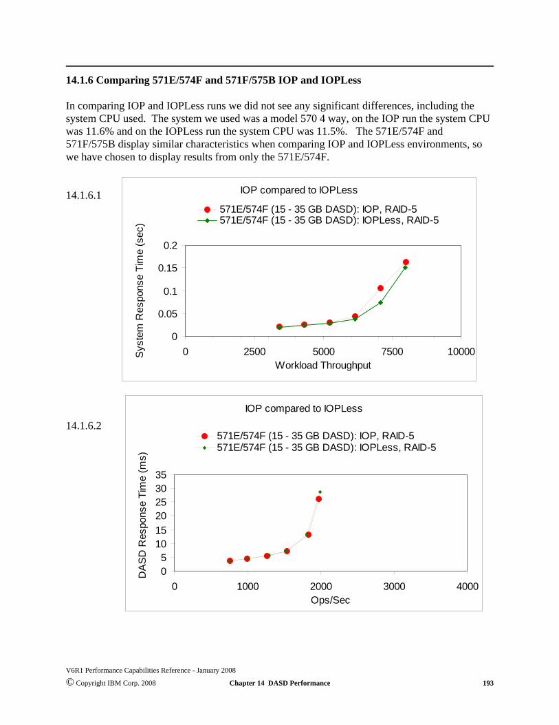
14.1.6 Comparing 571E/574F and 571F/575B IOP and IOPLess

In comparing IOP and IOPLess runs we did not see any significant differences, including thesystem CPU used. The system we used was a model 570 4 way, on the IOP run the system CPUwas 11.6% and on the IOPLess run the system CPU was 11.5%. The 571E/574F and571F/575B display similar characteristics when comparing IOP and IOPLess environments, sowe have chosen to display results from only the 571E/574F.

14.1.6.1

14.1.6.2



IOP compared to IOPLess

0

0.05

0.1

0.15

0.2

0 2500 5000 7500 10000

571E/574F (15 - 35 GB DASD): IOP, RAID-5571E/574F (15 - 35 GB DASD): IOPLess, RAID-5

Workload Throughput

Sys

tem

Res

pons

e Ti

me

(sec

)

IOP compared to IOPLess

05

101520253035

0 1000 2000 3000 4000

571E/574F (15 - 35 GB DASD): IOP, RAID-5571E/574F (15 - 35 GB DASD): IOPLess, RAID-5

Ops/Sec

DA

SD

Res

pons

e Ti

me

(ms)

14.1.7 Comparing 571E/574F and 571F/575B RAID-5 and RAID-6 and Mirroring

System i protection information can be found at http://www.redbooks.ibm.com/ in the currentSystem i Handbook or the Info Center http://publib.boulder.ibm.com/iseries/ . When comparingRAID-5, RAID-6 and Mirroring we are interested in looking at the strength of failure protectionvs storage capacity vs the performance impacts to the system workloads.

A model 570 4 way system with 48 GB of mainstore memory was used for the following. Firstcomparing characteristics of RAID-5 and RAID-6; a customer can use Operations Navigator tobetter control the number of DASD in a RAID set but for this testing we signed on at DST andused default available to turn on our protection schemes. When turning on RAID-5 the systemconfigured two RAID sets under our IOA, one with 9 DASD and one with 6 DASD with a totaldisk capacity of 457 GB. For RAID-6 the system created one RAID set with 15 DASD and acapacity of 456 GB. This would generally be true for most customer configurations.

As you look at our run information you will notice that the performance boundaries of RAID-6on the 571E/574F is about the same as the performance boundaries of our 2780/574F configuredusing RAID-5, so better protection could be achieved at current performance levels.

Another point of interest is that as long as a system is not pushing the boundaries, performance issimilar in both the RAID-5 and RAID-6 environments. RAID-6 is overwhelmed quicker thanRAID-5, so if RAID-6 is desired for protection and the system workloads are approaching theboundaries, DASD and IOAs may need to be added to the system to achieve the desiredperformance levels. NOTE: If customers need better protection greater than RAID-5 it might beworth considering the IOA level mirroring information on the following page.

14.1.7.1

14.1.7.2



RAID-5 Compared to RAID-6

050

100

0 1000 2000 3000 4000

2780/574F (15 - 35 GB DASD): IOP, RAID-5571E/574F (15 - 35 GB DASD): IOPLess, RAID-5571E/574F (15 - 35 GB DASD): IOPLess, RAID-6

Ops/SecDA

SD

Res

pons

e Ti

me

(ms)

RAID-5 Compared to RAID-6

0

0.1

0.2

0 2000 4000 6000 8000 10000

2780/574F (15 - 35 GB DASD): IOP, RAID-5571E/574F (15 - 35 GB DASD): IOPLess, RAID-5571E/574F (15 - 35 GB DASD): IOPLess, RAID-6

Workload ThroughputSys

tem

Res

pons

e Ti

me

(sec

)

http://www.redbooks.ibm.com/

http://publib.boulder.ibm.com/iseries/

In comparing Mirroring and RAID one of the concerns is capacity differences and the hardwareneeded. We tried to create an environment where the capacity was the same in bothenvironments. To do this we built the same size database on “15 35GB DASD using RAID-5”and “14 70GB DASD using Mirroring spread across 2 IOAs”. The protection in the Mirroredenvironment is better but it also has the cost of an extra IOA in this low number DASDenvironment. For the 30 DASD and 60 DASD environments the number of IOAs needed isequal.

14.1.7.3

14.1.7.4



RAID-5 compared to Mirroring

00.050.1

0.150.2

0.25

0 5000 10000 15000 20000 25000 30000 35000 40000

571E/574F (15 - 35 GB DASD): IOPLess, RAID-5571E (14 - 70 GB DASD): IOPLess, 7 Mirrored Pairs 2 IOAs571E (30 DASD): IOPLess, 15 Mirrored Pairs 2 IOAs571E/574F (30 DASD): IOPLess, RAID-5 2 IOAs571E (60 DASD): IOPLess, 30 Mirrored Pairs 4 IOAs571E/574F (60 DASD): IOPLess, RAID-5 4 IOAs

Workload Throughput

Sys

tem

Res

pons

e Ti

me

(sec

)

RAID-5 compared to Mirroring

0

10

20

30

40

0 2000 4000 6000 8000 10000

571E/574F (15 - 35 GB DASD): IOPLess, RAID-5571E (14 - 70 GB DASD): IOPLess, 7 Mirrored Pairs 2 IOAs571E (30 DASD): IOPLess, 15 Mirrored Pairs 2 IOAs571E/574F (30 DASD): IOPLess, RAID-5 2 IOAs571E (60 DASD): IOPLess, 30 Mirrored Pairs 4 IOAs571E/574F (60 DASD): IOPLess, RAID-5 4 IOAs

Ops/Sec

DA

SD

Res

pons

e Ti

me

(ms)

14.1.8 Performance Limits on the 571F/575B

In the following charts we try to characterize the 571F/575B in different DASD configuration.The 15 DASD experiment is used to give a comparison point with DASD experiments fromchart 14.1.5.1 and 14.1.5.2. The 18, 24 and 36 DASD configurations are used to help in thediscussion of performance vs capacity.

Our DASD IO workload scaled well from 15 DASD to 36 DASD on a single 571F/575B

14.1.8.1

14.1.8.2



571F/575B Scaling

0

0.05

0.1

0.15

0.2

0 5000 10000 15000 20000

571F/575B (15 DASD): IOPLess, RAID-5571F/575B (1 IOA 18 DASD 3 cages each off 1 571F port): IOPLess, RAID-5571F/575B (24 DASD): IOPLess, RAID-5571F/575B (36 DASD 1 IOA 12 DASD off each 571F port): IOPLess, RAID-5571F/575B (36 DASD 2 IOAs 6 DASD off each 571F port): IOPLess, RAID-5

Workload Throughput

Sys

tem

Res

pons

e Ti

me

(sec

)

571F/575B Scaling

05

1015202530

0 1,000 2,000 3,000 4,000 5,000 6,000

571F/575B (15 DASD): IOPLess, RAID-5571F/575B (1 IOA 18 DASD 3 cages each off 1 571F port): IOPLess, RAID-5571F/575B (24 DASD): IOPLess, RAID-5571F/575B (36 DASD 1 IOA 12 DASD off each 571F port): IOPLess, RAID-5571F/575B (36 DASD 2 IOAs 6 DASD off each 571F port): IOPLess, RAID-5

Ops/Sec

DAS

D R

espo

nse

Tim

e (m

s)

14.1.9 Investigating 571E/574F and 571F/575B IOA, Bus and HSL limitations.

With the new DASD controllers and IOPLess capabilities, IBM has created many new optionsfor our customers. Customers who needed more storage in their smaller configurations can nowgrow. With the ability to add more storage into an HSL loop the capacity and performance havethe potential to grow. In the past a single HSL loop only allowed 6 5094 towers with 45 DASDper tower, giving a loop a capacity of 270 DASD, with the new DASD controllers that capacityhas grown to 918 DASD. With the new configurations, you can see that 500 and even 600DASD could make better use of the HSL loop's potential as opposed to the current limit of 270DASD. Customer environments are unique and these options will allow our customers to look attheir space, performance, and capacity needs in new ways.

With the ability to attach so much more DASD to existing towers we want to try to characterizewhere possible bottlenecks might exist. The first limits are the IOAs and we have attempted tocharacterize the 571E/574F and 571F/575B in RAID and Mirroring environments. The nextlimit will be the buses in a single tower. We are using a large file concurrent RSTLIB operationsfrom multiple virtual tape drives located on the DASD in the target HSL loop, to try to helpcharacterize the Bus and HSL limits. The tower is by itself in a single HSL loop, with all theDASD configured into a single user ASP, and RAID-5 activated on the IOAs.

As the scenarios progress 2 then 3 towers are added up to 6 in the HSL loop. All 6 have 3571E/574F’s controlling the 45 DASD in the 5094 towers and 3 571F/575B IOAs controlling108 DASD in #5786 EXP24 Disk Drawer. Multiple Virtual tape drives were created in the userASP. The 3 other HSL loops contained the system ASP where the data is written to. We usedthree HSL loops to prevent the destination ASP from being the bottleneck. The system was a570 ML16 way with 256 GB of memory and originating ASP contained 916 DASD units on571E/574F and 571F/575B IOAs. Restoring from the virtual tape would create runs of 100%reads from the ASP on the single loop. The charts show the maximum throughput we were ableto achieve from this workload.

NOTE: This is a DASD only workload. No other IOAs such as communication IOAs werepresent.



14.1.9.1

14.1.9.2



Large Block READs on a Single 5094 Tower in an HSL Loop

1_To

wer

81

_DAS

D3_

571E

&1_

571F

1_To

wer

117_

DASD

3_57

1E &

2_57

1F

1_To

wer

153_

DASD

3_57

1E &

3_57

1F

Large Block READs on Multiple 5094 Towers in a Single HSL Loop

1_To

wer

3_57

1E_&

_3_5

71F

153_

DAS

D

2_To

wer

s6_

571E

_&_6

_571

F30

6_DA

SD

3_To

wer

s9_

571E

_&_9

_571

F45

9_DA

SD

4_To

wer

s12

_571

E_&_

12_5

71F

612_

DAS

D

5_To

wer

s15

_571

E_&_

15_5

71F

765_

DAS

D

6_To

wer

s18

_571

E_&_

18_5

71F

918_

DAS

D

14.1.10 Direct Attach 571E/574F and 571F/575B Observations

We did some simple comparison measurements to provide graphical examples for customers toobserve characteristics of new hardware. We collected performance data using CollectionServices and Performance Explorer to create our graphs after running our DASD IO workload(small block reads and writes).

IOP vs IOPLess: no measurable difference in CPU or throughput.

Newer models of DASD are U320 capable and with the new IOAs can improve workloadthroughput with the same number of DASD or even less in some workload situations.

IOA’s 571E/574F and the 571F/575B achieved up to 25% better throughput at the 40% DASDSubsystem Utilization point than the 2780/574F IOA. The 571E/574F and 2780/574F weremeasured with 15 DASD units in a 5094 enclosure. The 571F/575B IOAs attached to #5786EXP24 Disk Drawers.

System Models and Enclosures: Although an enclosure supports the new DASD or new IOA,you must ensure the system is configured optimally to achieve the increased performancedocumented above. This is because some card slots or backplanes may only support the PCIprotocol versus the PCI-X protocol. Your performance can vary significantly from ourdocumentation depending upon device placement. For more information on card placementrules see the following link:i5/OS V5R2: http://www.redbooks.ibm.com/redpapers/pdfs/redp3638.pdfi5/OS V5R3, V5R4: http://www.redbooks.ibm.com/redpapers/pdfs/redp4011.pdf

Conclusions: There can be great benefits in updating to new hardware depending upon thesystem workload. Most DASD intense workloads should benefit from the new IOAs available.Large block operations will greatly benefit from the 5094/5294 feature code #6417/9517enclosures in combination with the new IOA’s and DASD units.Note: The #6417/9517 provides a faster HSL-2 interface compared to the #2887/9877 and isavailable for I/O attached to POWER-5 based systems





14.2 New in V5R4M5

14.2.1 9406-MMA CEC vs 9406-570 CEC DASD



0.020.04

0.060.080.1

0.12

0.140.16

0 200 400 600 800 1000 1200

9406-MMA 4 way 6 433B 70 GB DASD Mirrored "No Cache"9406-570 4 way 6 4327 70 GB DASD Mirrored "No Cache"9406-570 4 way 6 4327 70 GB DASD Mirrored "With Cache"

Workload Throughput

Sys

tem

Res

pons

e Ti

me

(sec

)

02468

10121416

0 100 200 300 400 500 600

9406-MMA 4 way 6 433B 70 GB DASD Mirrored "No Cache"9406-570 4 way 6 4327 70 GB DASD Mirrored "No Cache"9406-570 4 way 6 4327 70 GB DASD Mirrored "With Cache"

Ops/Sec

DA

SD

Res

pons

e Ti

me

(ms)

14.2.2 RAID Hot Spare

For the following test, the IO workload was setup to run for 14 hours. About 5 hours afterstarting A DASD was pulled from the configurations. This forced a RAID set rebuild.



0.02

0.05

0.08

0.11

0.14

5000 6000 7000 8000 9000 10000 11000 12000 13000

9406-570 4 way 24 4328 140 GB RAID5 24 active9406-570 4 way 24 4328 140 GB RAID5 22 active 2 Hot Spares9406-570 4 way 24 4328 140 GB RAID6 24 active9406-570 4 way 24 4328 140 GB RAID6 22 active 2 Hot Spares

Workload Throughput

Sys

tem

Res

pons

e Ti

me

(sec

)

00.20.40.60.8

11.21.41.61.8

2 4 6 8 10 12

570 4 way 24 4328 140 GB DASD RAID5 2 Hot Spares

Runtime in Hours

Syst

em R

espo

nse

Tim

e (s

ec)

14.2.3 12X Loop Testing

A 9406-MMA 8 Way system with 96 GB of mainstore and 396 DASD in #5786 EXP24 DiskDrawer on 3 12X loops for the system ASP were used, ASP 2 was created on a 4th 12X loop byadding 5796 system expansion units with 571F IOAs attaching 36 4327 70 GB DASD in #5786EXP24 Disk Drawer with RAID5 turned on. I created a virtual tape drive in ASP2 and I used a320GB file to save to the tape drive for this test.

When I completed the testing up to 288 DASD on 8 IOAs, I moved the 12X loop to the other 12X GX adapter in the CEC and ran the test again and saw no difference in the testing betweenthe two loops. The 12X loop is rated for more throughput than the DASD configuration wouldallow for. So the test isn’t a tell all about the 12X loops capabilities only a statement of supportto the maximum number of 571F IOAs allowed in the loop.



0

200

400600

800

1000

12001400

1600

1800

1 2 3 4 5 6 7 8

Number of 571F IOAs

GB

/HR

12X Loop testing from 1 571F to 8 571F IOAs with 36 DASD off each 571F

14.3 New in V6R1M0

14.3.1 Encrypted ASP

More CPU and memory may be needed to achieve the same performance once encryption isenabled.



Non Encrypted ASP vs Encrypted ASP

0

0.05

0.1

0.15

0.2

2000 4000 6000 8000 10000 12000 14000

DASD/IO Workload Throughput

Syst

em R

espo

nse

Tim

e (m

s)

9406 MMA 4 Way 571F w ith 24 DASD Non Encrypted ASP

9406 MMA 4 Way 571F w ith 24 DASD Encrypted ASP


0

5

10

15

20

25

30

35

0 500 1000 1500 2000 2500 3000 3500

Ops/sec

Das

d R

espo

nse

Tim

e (m

s)

9406 MMA 4 Way 571F with 24 DASD Non Encrypted ASP

9406 MMA 4 Way 571F with 24 DASD Encrypted ASP




0

5

10

15

20

25

6000 7300 8600 9800

Workload Throughput

CPU

9406 MMA 4 Way 571F with 24 DASD Non Encrypted ASP9406 MMA 4 Way 571F with 24 DASD Encrypted ASP

14.4 SAN - Storage Area Network (External)

There are many factors to consider when looking at external storage options, you can get moreinformation through your IBM representative and the white papers that are available to them at thefollowing locations.

White paper on the DS8300Http://tucgsa.ibm.com//gsa/home/s/s/sspadmin/web/public/docs/disk/white%20papers/ds8300iserieswhitepaper_011206.pdf

White paper on the DS6000Http://w3-1.ibm.com/sales/systems/portal/_s.155/254?navID=f320s260&geoID=All&prodID=IBM%20Systems&docID=ditlDS6800PerfWPSystemi



Http://tucgsa.ibm.com//gsa/home/s/s/sspadmin/web/public/docs/disk/white%20papers/ds8300ise

Http://w3-1.ibm.com/sales/systems/portal/_s.155/254?navID=f320s260&geoID=All&prodID=I

14.5 V6R1 -- VIOS and IVM Considerations

Beginning in V6R1, i5/OS will participate in a new virtualization strategy by becoming a clientof the VIOS product. Customers will view the VIOS product two different ways:

On blade products, through the regular configuration tool IVM (which includes an easy touse interface to VIOS).On traditional (non-blade) products, through a combination of HMC and the VIOS commandline.

The blade products have a simpler interface which, on our testing, appear to be sufficient for theenvironments involved. On blades, customers are restricted to a single set of 16 logical units(which i5/OS perceives as if they were physical drives). This substantially reduces the numberand value of tuning options. It is possible for blade-based customers to use the VIOS commandline. However, we did not discover the need to do so and do not think most customers will needto either. The tuning available from IVM proved sufficient and should be preferred for its easeof use when it is workable.

Customers should strongly consider their disk requirements here and consult with their supportteams before ordering. Customers with more sophisticated disk-based requirements (or, simply,larger numbers of disks) should choose systems that allow a greater number of LUNs andthereby enable more substantial tuning options provided from the VIOS command line. No hardand fast rules are possible here and we again emphasize that one consult with their support teamon what will work for them. However, as a broad rule of thumb, customers with 200 or morephysical drives very likely need something beyond the 16 LUNs provided by the IVMenvironment. Customers below 100 physical disks can, in most cases, get by with IVM.Customers with 50 or fewer very likely will do just fine with IVM.



14.5.1 General VIOS Considerations

14.5.1.1 Generic Concepts

520 versus 512. Long time i5/OS users know that i5/OS disks are traditionally configured with520 byte sectors. The extra eight bytes beyond the 512 used for data are used for variouspurposes by Single Level Store.

For a variety of reasons, VIOS will always surface 512 byte sectors to i5/OS whatever the actualsector size of the disk may be. This means that 520 byte sectors must be emulated within 512byte sectors when using disks supported by VIOS. This is done, simply enough, by reading nine512 byte data sectors for every eight sectors of actual data and placing the Single Level Storeinformation within the extra sector. Since all disk operations are controlled by Single Levelstore in an i5/OS system, there are no added security implications from this extra sector,provided standard, sensible configuration practices are followed just as they would be for regular520 byte devices.

However, reading nine sectors when only eight contain data will cost some performance, most ofit being the sheer cost of the extra byte transfer of the extra sector. The gains are the standardones of virtualization -- one might be able to share or re-purpose existing hardware for System i'suse in various ways.

Note carefully that some "512" byte sectored devices actually have a range of sizes like 522,524, and others. Confusingly for us, the industry has gone away from strictly 512 byte sectorsfor some devices. They, too, have headers that consume extra bytes. However, as noted above,these extra bytes are not available for i5/OS and so, for our purposes, they should be consideredas if they were 512 byte sectored, because that is what i5/OS will see. Some configuration tools,however, will discuss "522 byte" or whatever the actual size of the sectors is in variousinterfaces (IVM users will not see any of this).

VIOS will virtualize the devices. Many configuration options are available for mapping physicaldevices, as seen by VIOS, to virtual devices that VIOS will export to DST and Single LevelStore. Much more of this will be done by the customer than was done with internal disks.Regardless of whether the environment is blades or traditional, it is important to make goodchoices here. Even though there is much functional freedom, many choices are not optimized forperformance or optimized in an i5/OS context. Moreover, nearly as a matter of sheer physics,some choices, once made, cannot be much improved without very drastic steps (e.g. dedicatingthe system, moving masses of data around, etc.). Choosing the right configuration in the firstplace, in other words, is very important. Most devices, especially SAN devices, will have “BestPractices” manuals that should be consulted.



14.5.1.2 Generic Configuration Concepts

There are several important principles to keep track of in terms of getting good performance.Most of the following are issues when the disks are configured. A great many problems can beeliminated (or, created) when the drives are originally configured. The exact nature of some ofthese difficulties might not be easily predicted. But, much of what follows will simply avoidtrouble at no other cost.

1. Ensure that RAID protection is performed as close to the physical device as possible . Thisis typically done out at an I/O adapter level or on the external disk array product. This meansthat either the external disk's configuration tools or (for internal disks assigned to VIOS) VIOS'tools will be used to create RAID configurations (RAID5, RAID10, or RAID1). When this isdone, as far as i5/OS disk status displays are concerned, the resulting virtual drives appear to be"unprotected." It might be superficially reassuring to have i5/OS do the protection (if i5/OSeven permits it). WRKDSKSTS would then show the protection on that path. DST/SST diskconfiguration functions would show the protection, too. However, it is better to put up withwhat appears to i5/OS's disk status routines to be unprotected devices (which are, after all,actually protected) than to take on the performance problems of doing this under i5/OS. RAIDrecovery procedures will have to be pursued outside of i5/OS in any event, so the protection mayas well go where the true physicality is understood (either in VIOS or the external disk arrayproduct). Note also that you also want to configure things so that the outboard devices, rather than VIOS,do the RAID protection whenever possible. This enables I/O to flow directly from the device toi5/OS as directed by VIOS.

High Availability scenarios also need to be considered. In some cases, to enable appropriateredundancy, it may be necessary to do the protection a little farther away from the device (e.g.spread over a couple of adapters) so as to enable the proper duplexing for high availability. Ifthis applies to you, consult the documentation. Some external storage devices have extensiveduplexing within themselves, for instance, which could allow one to keep the protection close tothe device after all.

2. Recognize that Internal Disks remain the "gold standard" for performance. We haveconsistently measured external disks as having less performance than 520 byte, internallyattached disks. However, the loss of throughput, with proper configuration, is not a majorconcern. What is harder to control is response time. If you have sensitivity to response time,consider internal disks more strongly.



3. Prefer external disks attached directly to i5/OS over those attached via VIOS This isbasically a statement of the Fibre Channel adapter and who owns it. In some cases, it affectswhich adapter is purchased. If you do not need to share a given external disk's resources withnon-i5/OS partitions, and the support is available, avoiding VIOS altogether will give betterperformance. First, the disks will usually have 520 byte support. Second, the i5/OS support willknow the device it is dealing with. Third, VIOS will typically run as a separate partition. If yourun VIOS as your first shared partition, simply turning on shared support costs about five toeight percent overall. The alternative, a dedicated partition for VIOS, would be a nice thing toavoid if possible. If you would not have used shared processor support otherwise, or would haveto give VIOS a whole processor or more otherwise, this is a consideration.

4. Prefer standard i5/OS internal disks to VIOS internal disks. This describes who should owna given set of internal disks. If there is a choice, giving the available internal disks to i5/OSinstead of going through VIOS will result in noticeably better performance. VIOS is a better fitfor external disk products that do not support the i5/OS 520 byte sector. The VIOS case wouldinclude internal disks that came originally from pSeries or System p. However, one shouldinvestigate those devices also. If those devices support 520 byte sectors (or, alternatively, if it isstated they are supported by i5/OS), they should be reconfigured instead as native i5/OS internaldisks. It should be exceptional to use VIOS for internal disks.

5. Prefer RAID 1 or RAID 10 to RAID 5. We are now beginning to generally recommendRAID 1 ("mirroring") or RAID 10 (a "mirroring" variant) for disks generally in On-lineTransaction Processing (OLTP) environments. OLTP environments have long had to deal withconfigurations based on total arm count, not capacity as such. If that applies to you, you haveextra space that is of marginal value. Those in this situation can nowadays use the same numberof arms deployed as RAID 1 or RAID 10 to gain increased performance. This is at least as truefor external disks as it is for internal disks. Note that in this recommendation, one deploys thesame arm count -- just deploys them differently, trading unused space for performance. Alsonote that if one goes this route, two physical disks per RAID 10 or RAID 1 set is better than alarger number of disks per RAID 1 or RAID 10 set. (See also “Ensure, within reason” below).

6. For VIOS, Prefer External Disks (SAN disks) to Internal Disks. SAN disks will havegreater flexibility and better tuning options than internal disks. Accordingly, when there is achoice, VIOS is best used for external disks.

7. Separate Journal ASPs from other ASPs. Generally, we have long recommended that agiven set of data base files (aka SQL tables) keep its set of journal receivers in a separate ASPfrom the data base ASP or ASPs. With VIOS, we recommend that this continue to the extentfeasible. It may be necessary to share things like Fibre Channel links, but it should be possibleto have separate physical devices at the very least. To the extent possible, arrange for journal touse its own internal busses also (of whatever sort the device provides).



8. Ensure, within reason, a reasonable number of virtual disks are created and madeavailable to i5/OS. One is tempted to simply lump all the storage one has in a virtualenvironment into a couple (or even one) large virtual disk. Avoid this if at all possible.

For traditional (non-blade) systems: There is a great deal of variability here, sogeneralizations are difficult. However, in the end, favor virtual disks that are within a binaryorder of magnitude or two of the physical disk sizes. Make each them as close to the same size ifpossible. In any case, strive to have half a dozen or more in an ASP if you can. Years of systemtuning (at all levels) tacitly expect a reasonable number of devices, so it makes sense to provide abunch. You don't need a count larger than the physical device count, however, unless the devicecount is very small.

For blades-based systems: You only have 16 LUNs available. However, you should usea good fraction of them rather than merely one or two. In our tests, we tended to use twelve tosixteen LUNs. One wishes a sufficient number for i5/OS to work with -- one wishes also tosegregate physical devices between ASPs to the extent feasible.

9. Prefer Symmetrical Configurations. To the extent possible, we have found that physicalsymmetry pays off more than we have seen before. Balancing the number of physical disks asmuch as possible seems to help. Strive to have uniform LUN sizes, uniform number of disks ineach RAID set, balance (at least at the static configuration level) between the various internaland external busses, etc. To the extent practical, the user should strive for even numbers ofitems.

10. In general, do not share the same physical disk with multiple partitions. Only If you arerunning some minimal i5/OS partition (say, a very small Domino partition or perhaps a middletier partition that has no local data base), should you consider strategies where i5/OS is sharingphysical disks with other partitions. For more traditional application sets (whether a traditionalsystem or a blade) you'll have a data base or large enough data contents generally to give eachi5/OS partition its own physical devices. Once you get to multiple devices, sharing them withother partitions will lead to performance problems as the two partitions fight (in mutualignorance) for the same arm, which may increase seek time (at least) a little to a lot. Servicetime could be adversely affected as well.

11. To the extent possible, think multiple VIOS partitions for multiple i5/OS partitions. If thephysical disks deserve segmentation, multiple VIOS partitions may also be justified. The mainissue is load. If the i5/OS partitions are small (under two CPUs), then you're probably better offwith a shared VIOS partition hosting a couple of small i5/OS partitions. As the i5/OS partitionsgrow, it will be possible to justify dedicated VIOS partitions. Our current measurements suggestone VIOS processor for every three i5/OS processors, but this will vary by the application.



14.5.1.3 Specific VIOS Configuration Recommendations -- Traditional (non-blade)Machines

1. Avoid volume groups if possible. VIOS "hdisks" must have a volume identifier (PVID).Creating a volume group is an easy way to assign one and some literature will lead you to do itthat way. However, the volume group itself adds overhead for no particular value in a typicali5/OS context where physical volumes (or, at least, RAID sets) are exported as a whole withoutany sort of partitioning or sub-setting. Volume groups help multiple clients share the samephysical disks. In an i5/OS setting, this is seldom relevant and the overhead volume groupsemploy is therefore not needed. It is better to assign a PVID by simply changing the attribute ofeach individual hdisk. For instance, the VIOS command: chdev -dev hdisk03 -attrpv=yes will assign a PVID to hdisk3.

2. For VIOS disks, use available location information to aid your RAID planning. To obtainRAID sets in i5/OS, you simply point DST at particular groups you want and i5/OS decideswhich disks go together. Under VIOS, for internal disks, you have to do this yourself. Thenames help show you what to do. For instance, suppose VIOS shows the following for a set ofinternal disks:

Name Location State Description Size pdisk0 07-08-00-2,0 Active Array Member 35.1GB pdisk1 07-08-00-3,0 Active Array Member 35.1GB pdisk2 07-08-00-4,0 Active Array Member 35.1GB pdisk3 07-08-00-5,0 Active Array Member 35.1GB pdisk4 07-08-00-6,0 Active Array Member 35.1GB pdisk5 07-08-01-0,0 Active Array Member 35.1GB pdisk6 07-08-01-1,0 Active Array Member 35.1GB

Here, it turns out that these particular physical disks are on two internal SCSI busses (00 and 01)and have device IDs of 2, 3, 4, 5, and 6 on SCSI bus 00 and device IDs of 0 and 1 on SCSI bus01. If this was all there was, a three disk RAID set of pdisk0, pdisk1, and pdisk5 would be agood choice. Why? Because pdisk0 and 1 are on internal SCSI bus 00 and the other one is oneSCSI bus 01. That provides a good balance for the available drives. This could also be repeatedfor pdisk2, pdisk3, pdisk4, and pdisk6. This would result in two virtual drives being created torepresent the seven physical drives. The fact that these are two RAID5 disk sets (of three andfour physical disks, respectively) would be unknown to i5/OS, but managed instead by VIOS.One or may be two virtual SCSI busses would be required to present them to i5/OS by VIOS.

A large configuration could provide for RAID5 balance over even more SCSI busses (real andvirtual).

On external storage, the discussion is slightly more complicated, because these products tend topackage data into LUNs that already involve multiple physical drives. Your RAID set workwould have to use whatever the external disk storage product gives you to work with in terms ofnaming conventions and what degree of control you have available to reflect favorable physicalboundaries. Still, the principles are the same.



3. Limited number of virtual devices per virtual SCSI adapter. You will have to configuresome number of virtual SCSI adapters so that VIOS can provide a path for i5/OS to talk to VIOSas if these were really physical SCSI devices. These adapters, in turn, implement some existingrules, so that only 16 virtual disks can be made part of a given virtual adapter. You probablywould not want to exceed this limit anyway. Note that the virtual adapters need not relate tophysical boundaries of the various underlying devices. The main issue is to balance the load.You may be able to segregate data base and journal data at this level. Note also that in a properconfiguration, the virtual SCSI adapters will carry command traffic only. The actual data DMAwill be direct to the i5/OS partition.

4. VIOS and Shared Processors. On the whole, dedicated VIOS processors will work betterthan shared processors, especially as the i5/OS partition needs three or more CPUs itself. If youdo not need shared processors for other reasons, experiment and see if dedicated VIOSprocessors work better. In fact, it might be an experiment worth running even if you have sharedprocessors configured generally.

5. VIOS and memory. VIOS arranges for the DMA to go directly to the i5/OS memory (withthe help of PHYP and i5/OS to ensure integrity). This means that actual data transfer will not gothrough VIOS. It only needs enough main storage to deal with managing disk traffic, not thedata the traffic itself consumes. Our current measurements suggests that 1 GB of main storage isthe minimum recommended. Other work suggest that unless substantial virtual LAN is involved,between 1 GB and 2 GB tends to suffice at the 1 to 3 CPU ratio we typically measured.

6. VIOS and Queue Depth. Queue depth is a value you can change, so one can experiment tofind the best value, at least on a per IPL basis. VIOS tends the set the queue depth parameter tosmaller values. Especially if you follow our recommendations for the number of virtual disks,you will find values like 32 to work well for the device as a starting point. If you do that, youwill also want to set the queue depth for the adapter (usually called num_cmd_elems) to itslarger value, often 512. Consult the documentation.



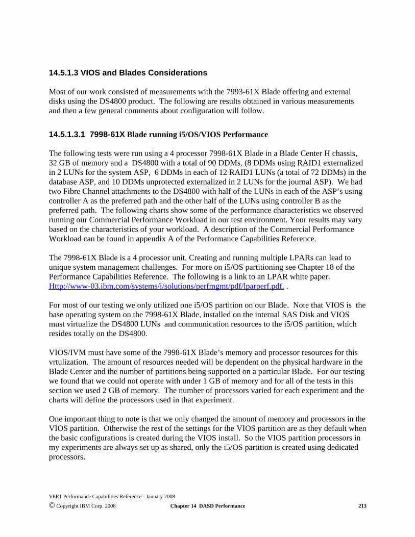
14.5.1.3 VIOS and Blades Considerations Most of our work consisted of measurements with the 7993-61X Blade offering and externaldisks using the DS4800 product. The following are results obtained in various measurementsand then a few general comments about configuration will follow.

14.5.1.3.1 7998-61X Blade running i5/OS/VIOS Performance

The following tests were run using a 4 processor 7998-61X Blade in a Blade Center H chassis,32 GB of memory and a DS4800 with a total of 90 DDMs, (8 DDMs using RAID1 externalizedin 2 LUNs for the system ASP, 6 DDMs in each of 12 RAID1 LUNs (a total of 72 DDMs) in thedatabase ASP, and 10 DDMs unprotected externalized in 2 LUNs for the journal ASP). We hadtwo Fibre Channel attachments to the DS4800 with half of the LUNs in each of the ASP’s usingcontroller A as the preferred path and the other half of the LUNs using controller B as thepreferred path. The following charts show some of the performance characteristics we observedrunning our Commercial Performance Workload in our test environment. Your results may varybased on the characteristics of your workload. A description of the Commercial PerformanceWorkload can be found in appendix A of the Performance Capabilities Reference.

The 7998-61X Blade is a 4 processor unit. Creating and running multiple LPARs can lead to unique system management challenges. For more on i5/OS partitioning see Chapter 18 of thePerformance Capabilities Reference. The following is a link to an LPAR white paper. Http://www-03.ibm.com/systems/i/solutions/perfmgmt/pdf/lparperf.pdf. .

For most of our testing we only utilized one i5/OS partition on our Blade. Note that VIOS is thebase operating system on the 7998-61X Blade, installed on the internal SAS Disk and VIOSmust virtualize the DS4800 LUNs and communication resources to the i5/OS partition, whichresides totally on the DS4800.

VIOS/IVM must have some of the 7998-61X Blade’s memory and processor resources for thisvrtulization. The amount of resources needed will be dependent on the physical hardware in theBlade Center and the number of partitions being supported on a particular Blade. For our testingwe found that we could not operate with under 1 GB of memory and for all of the tests in thissection we used 2 GB of memory. The number of processors varied for each experiment and thecharts will define the processors used in that experiment.

One important thing to note is that we only changed the amount of memory and processors in theVIOS partition. Otherwise the rest of the settings for the VIOS partition are as they default whenthe basic configurations is created during the VIOS install. So the VIOS partition processors inmy experiments are always set up as shared, only the i5/OS partition is created using dedicatedprocessors.



Http://www-03.ibm.com/systems/i/solutions/perfmgmt/pdf/lparperf.pdf

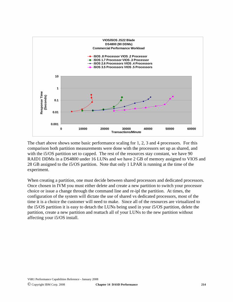
The chart above shows some basic performance scaling for 1, 2, 3 and 4 processors. For thiscomparison both partition measurements were done with the processors set up as shared, andwith the i5/OS partition set to capped. The rest of the resources stay constant, we have 90RAID1 DDMs in a DS4800 under 16 LUNs and we have 2 GB of memory assigned to VIOS and28 GB assigned to the i5/OS partition. Note that only 1 LPAR is running at the time of theexperiment.

When creating a partition, one must decide between shared processors and dedicated processors.Once chosen in IVM you must either delete and create a new partition to switch your processorchoice or issue a change through the command line and re-ipl the partition. At times, theconfiguration of the system will dictate the use of shared vs dedicated processors, most of thetime it is a choice the customer will need to make. Since all of the resources are virtualized tothe i5/OS partition it is easy to detach the LUNs being used in your i5/OS partition, delete thepartition, create a new partition and reattach all of your LUNs to the new partition withoutaffecting your i5/OS install.



VIOS/i5OS JS22 BladeDS4800 (90 DDMs)

Commercial Performance Workload

0.001

0.01

0.1

1

10

0 10000 20000 30000 40000 50000 60000Transactions/Minute

Res

pons

e Ti

me

(Sec

onds

)

i5OS .8 Processor VIOS .2 Processori5OS 1.7 Processor VIOS .3 Processori5OS 2.6 Processors VIOS .4 Processorsi5OS 3.5 Processors VIOS .5 Processors

The following charts are a view of the characteristics we observed during our CommercialPerformance Workload testing on our JS22 Blade. The first chart shows the effect on theCommercial Performance Workload when we apply 3 Dedicated processors and then switch to 3shared processors.

In our experiment turning on shared processors had the following affects on performance for thatpartition.. The effect you observe will be dependent upon your environment and your workload.Our observation was that turning on shared processors had overhead associated with doing so.We then increased the amount of shared processors we assigned to the i5/OS partition, butcouldn’t recover the difference. The two charts that follow show the CPU usage on the i5/OSpartition and the underlying VIOS partition.



VIOS/i5OS 7998-61X 4 WAY Blade DS4800 (90 DDMs)

Commercial Performance Workload

0.001

0.01

0.1

1

10

20000 25000 30000 35000 40000 45000 50000 55000 60000Transactions/Minute

Res

pons

e Ti

me

(Sec

onds

)

3 Dedicated Processors i5 Partition 1 Processor VIOS Partition3 Shared Processors i5 Partition 1 Processor VIOS Partition3.5 Shared Processors Partition i5 .5 Processor VIOS Partition

In following single partition Commercial Performance Workload runs the average VIOS CPUstayed under 40%, so we would still seem to have VIOS resource available but in a lot ofcustomer environments communications and other resources are also running and these resourceswill also be routed through VIOS.



i5/OS CPU Usage While Running the Commercial Performance Workload

10

20

30

40

50

60

70

80

90

100

20000 25000 30000 35000 40000 45000 50000 55000 60000Transactions/Minute

i5/O

S %

CPU

3 Dedicated Processors i5 Partition 1 Processor VIOS Partition

3 Shared Processors i5 Partition 1 Processor VIOS Partition

3.5 Shared Processors Partition i5 .5 Processor VIOS Partition

VIOS CPU Usage While Running the i5OS Commercial Performance Workload

10

20

30

40

50

20000 25000 30000 35000 40000 45000 50000 55000

Transactions/Minute

VIO

S %

CPU

3 Dedicated Processors i5 Partition 1 Processor VIOS Partition

3 Shared Processors i5 Partition 1 Processor VIOS Partition

3.5 Shared Processors Partition i5 .5 Processor VIOS Partition

The following chart shows two i5/OS partitions using 14GB of memory and 1.7 processors eachserved by 1 VIOS partition using 2GB of memory and .6 processors. The CommercialPerformance Workload was running the same amount of transactions on each of the partitionsfor the same time intervals. Although there is an observed cost for VIOS to manage multiplepartitions, VIOS was able to balance services to the two partitions. Experimenting with thenumber of processors and memory assigned to the partitions might yield a better environment forother workloads.



VIOS/i5OS JS22 2 Partition ExperimentsCommercial Performance Workload

0.0001

0.1001

0.2001

0 10000 20000 30000 40000 50000 60000Transactions/Minute

Res

pons

e Ti

me

(Sec

onds

)

1 of 2 i5/OS 1.7 Processor Partitions on a .6 Processor VIOS Partition Using 48 DS4800 DDMs2 of 2 i5/OS 1.7 Processor Partitions on a .6 Processor VIOS Partition Using 48 DS4800 DDMs1 Single i5?OS Partition 3.5 Processors on a .5 Processor VIOS Partition Using 96 4800 DDMs

14.5.1.3.2 Configuration Considerations

The Blades environment is simpler and therefore easier to configure.

1. The aggregate total of virtual disks (LUNs) will be sixteen at most. The previous generalconsiderations apply within this limit. Many customers will want to deploy between 12 and 16LUNs and maximize symmetry. Consult carefully with your support team on the choices here.This is the most important consideration as it is most difficult to change later. Properconfiguration of the physical disks into LUNs is probably the most important thing to get right ina blade environment as far as disk performance goes. Consult also any available Best Practicesmanuals for a given SAN.

2. The VIOS partition should be provided with between 1 and 2 GB of memory for disk-basedusage's. If virtual LAN is a substantial factor, more storage may be required.

3. See the above measurements for processor allocation.



Chapter 15. Save/Restore PerformanceThis chapter’s focus is on the System i platform. For legacy system models, older device attachmentcards, and the lower performing backup devices see the V5R3 performance capabilities reference.

Many factors influence the observable performance of save and restore operations. These factors include:The backup device models, number of DASD units the data is spread across, processors, LPARconfigurations, IOA used to attach the devices.Workload type: Large Database File, User Mix, Source File, integrated file system (Domino, NetworkStorage, 1 Directory Many Objects, Many Directory Many Objects.The use of data compression, data compaction, and Optimum Block Size (USEOPTBLK) Directory structure can have a dramatic effect on save and restore operations.

15.1 Supported Backup Device Rates

As you look at backup devices and their performance rates, you need to understand the backup devicehardware and the capabilities of that hardware. The different backup devices and IOAs have differentcapabilities for handling data for the best results in their target market. The following table containsbackup devices and rates. Later in this document the rates are used to help determine possibleperformance. A study of some customer data showed that compaction on their database file dataoccurred at a ratio of approximately 2.8 to 1. The database files used for the performance workloads werecreated to simulate that result.

#1. Software compression is used here because the hardware doesn’t support device compaction2.8100.03592E Fiber Channel1.5120.03580 Ultrium 4 Fiber Channel2.080.03580 Ultrium 3 Fiber Channel)2.840.03592J Fiber Channel 2.835.03580 Ultrium 22.818.05755 ½ High Ultrium-2 2.06.06258 4MM tape Drive2.012.06279 VXA-3202.06.0VXA-22.05.0SLR1002.04.0SLR60

2.8 #12.5SAS DVD-RAM2.8 #10.75 Write/2.8 ReadDVD-RAM

COMPACT Rate (MB/S)Backup DeviceTable 15.1.1 backup device speed and compaction information


© Copyright IBM Corp. 2008 Chapter 15. Save/Restore Performance 219

15.2 Save Command Parameters that Affect Performance

Use Optimum Block Size (USEOPTBLK)The USEOPTBLK parameter is used to send a larger block of data to backup devices that can takeadvantage of the larger block size. Every block of data that is sent has a certain amount of overhead thatgoes with it. This overhead includes block transfer time, IOA overhead, and backup device overhead. Theblock size does not change the IOA overhead and backup device overhead, but the number of blocksdoes. For example, sending 8 small blocks will result in 8 times as much IOA overhead and backupdevice overhead. This allows the actual transfer time of the data to become the gating factor. In thisexample, 8 software operations with 8 hardware operations essentially become 1 software operation with1 hardware operation when USEOPTBLK(*YES) is specified. The usual results are significantly lowerCPU utilization and the backup device will perform more efficiently.

Data Compression (DTACPR)Data compression is the ability to compress strings of identical characters and mark the beginning of thecompressed string with a control byte. Strings of blanks from 2 to 63 bytes are compressed to a singlebyte. Strings of identical characters between 3 and 63 bytes are compressed to 2 bytes. If a string cannotbe compressed a control character is still added which will actually expand the data. This parameter isusually used to conserve storage media. If the backup device does not support data compaction, thesystem i software can be used to compress the data. This situation can require a considerable amount ofCPU.

Data Compaction (COMPACT)Data compaction is the same concept as software compression but available at the hardware level. If youwish to use data compaction, the backup device you choose must support it.



15.3 Workloads

The following workloads were designed to help evaluate the performance of single, concurrent andparallel save and restore operations for selected devices. Familiarization with these workloads can help inunderstanding differences in the save and restore rates.

Database File related Workloads:The following workloads are designed to show some possible customer environments using databasefiles.

User Mix User Mix 3GB, User Mix 12GB - The User Mix data is contained in a single library andmade up of a combination of source files, database files, programs, command objects,data areas, menus, query definitions, etc. User Mix 12GB contains 49,500 objects andUser Mix 3GB contains 12,300 objects.

Source File Source File 1GB - 96 source files with approximately 30,000 members.

Large Database File Large File 4GB, 32GB, 64GB, 320GB - The Large Database File workload is asingle database file. The members in the 4GB and 32GB files are 4GB in size. TheMembers in the 64GB and 320GB files are 64GB in size.

Integrated File System related Workloads:Analysis of customer systems indicates about 1.5 to 1 compaction on the tape drives with integrated filesystem data. This is partly due to the fact that the i5/OS programs that store data in the integrated filessystem, do some disk management functions where they keep the IFS space cleaned up and compressed.And the fact that the objects tend to be smaller by nature, or are mail documents, HTML files or graphicobjects that don’t compact. The following workloads (1 Directory Many Objects, Many DirectoriesMany Objects, Domino, Network Storage Space) show some possible customer integrated file systemenvironments.

1 Directory Many objects This integrated file system workload consists of 111,111 stream files in asingle directory where the stream files have 32K of allocated space, 24K of which is data.Approximately 4 GB total sampling size.

Many Directories Many objects This integrated file system workload is 6 levels deep, 10directories wide where each directory level contains 10 directories resulting in a total of111,111 Directories and 111,111 stream files, where the stream files have 32K ofallocated space, 24K of which is data. Approximately 5 GB total sampling size.

Domino This integrated file system workload consists of a single directory containing 90 mailfiles. Each mail file is 152 MB in size. The mail files contain mail documents withattachments where approximately 75% of the 152 MB is attachments. Approximately 13GB total sampling size.

Network Storage Space This integrated file system workload consists of a Linux storage space ofapproximately 6 GB total sampling size.



15.4 Comparing Performance Data

When comparing the performance data in this document with the actual performance on your system,remember that the performance of save and restore operations is data dependent. If the same backupdevice was used on data from three different systems, three different rates may result.

The performance of save and restore operations are also dependent on the system configuration, mostdirectly affected by the number and type of DASD units on which the data is stored and by the type ofstorage IOAs being used.

Generally speaking, the Large Database File data that was used in testing for this document was designedto compact at an approximate 2.8 to1 ratio. If we were to write a formula to illustrate how performanceratings are obtained, it would be as follows:

((DeviceSpeed * LossFromWorkLoadType) * Compaction) = MB/Sec * 3600 = MB/HR /1000 = GB/HR.

But the reality of this formula is that the “LossFromWorkLoadType” is far more complex than describedhere. The different workloads have different overheads, different compaction rates, and the backupdevices use different buffer sizes and different compaction algorithms. The attempt here is to group theseworkloads as examples of what might happen with a certain type of backup device and a certainworkload.

Note: Remember that these formulas and charts are to give you an idea of what you might achieve froma particular backup device. Your data is as unique as your company and the correct backup devicesolution must take into account many different factors.

The save and restore rates listed in this document were obtained on a dedicated system. A dedicatedsystem is one where the system is up and fully functioning but no other users or jobs are running exceptthe save and restore operations. All processors and Memory were dedicated to the system and no partialprocessors were used. Other subsystems such as QBATCH are required in order to run concurrent andparallel operations. All workloads were deleted before restoring them again.



15.5 Lower Performing Backup Devices

With the lower performing backup devices, the devices themselves become the gating factor so the saverates are approximately the same, regardless of system CPU size (DVD-RAM).

25%Source File / 1 Directory Many Objects / Many Directories Many Objects55%User Mix / Domino / Network Storage Space95%Large Database FileAmount of LossWorkload Type

Table 15.5.1 Lower performing backup devices LossFromWorkLoadType Approximations (Save Operations)

Example for a DVD-RAM:DeviceSpeed * LossFromWorkLoad * Compression 0.75 * 0.95 = (.71) * 2.8 = (1.995) MB/S * 3600 = 7182 MB/HR = 7 GB/HR 0.75 * 0.95 = (.71) * No Compression * 3600 = 2556 MB/HR = 2.5 GB/HR

15.6 Medium & High Performing Backup Devices

Medium & high performing backup devices (SLR60, SLR100, VXA-2, VXA-320).

25%Source File / 1 Directory Many Objects / Many Directories Many Objects65%User Mix / Domino / Network Storage Space95%Large Database FileAmount of LossWorkload Type

Table 15.6.1 Medium performing backup devices LossFromWorkLoadType Approximations (Save Operations)

Example for SLR100:DeviceSpeed * LossFromWorkLoad * Compaction 5.0 * 0.95 = (4.75) * 2.0 = (9.5) MB/S * 3600 = 34200 MB/HR = 34 GB/HR

15.7 Ultra High Performing Backup Devices

High speed backup devices are designed to perform best on large files. The use of multiple high speedbackup devices concurrently or in parallel can also help to minimize system save times. See section onMultiple backup devices for more information (3580 Ultrium-2, 3580 Ultrium-3 (2Gb & 4Gb FiberChannel), 3592J, 3592E).

5%Source File / 1 Directory Many Objects / Many Directories Many Objects50% User Mix / Domino / Network Storage Space95%Large Database FileAmount of LossWorkload Type

Table 15.7.1 Higher performing backup devices LossFromWorkLoadType Approximations (Save Operations)

Example for 3580 ULTRIUM-2 Fiber:DeviceSpeed * LossFromWorkLoad * CompactionLG File 35.0 * 0.95 = (33.25) * 2.8= (93.1) MB/S *3600 = 335160 MB/HR = 335 GB/HRUserMix 35.0 * 0.50 = (17.5) * 2.8= (49) MB/S *3600 = 176400 MB/HR = 176 GB/HRSource 35.0 * 0.05 = (1.75) * 2.8= (4.9) MB/S *3600 = 17640 MB/HR = 17.6 GB/HR NOTE: Actual performance is data dependent, these formulas are for estimating purposes and maynot match actual performance on customer systems.



15.8 The Use of Multiple Backup Devices

Concurrent Saves and Restores - The ability to save or restore different objects from a singlelibrary/directory to multiple backup devices or different libraries/directories to multiple backup devices atthe same time from different jobs. The workloads that were used for the testing were Large DatabaseFile and User Mix from libraries. For the tests multiple identical libraries were created, a library for eachbackup device being used.

Parallel Saves and Restores - The ability to save or restore a single object or library/directory acrossmultiple backup devices from the same job. Understand that the function was designed to help thosecustomers, with very large database files which are dominating the backup window. The goal is toprovide them with options to help reduce that window. Large objects, using multiple backup devices,using the parallel function, can greatly reduce the time needed for the object operation to complete ascompared to a serial operation on the same object.

Concurrent operations to multiple backup devices will probably be the preferred solution for mostcustomers. The customers will have to weigh the benefits of using parallel verses concurrent operationsfor multiple backup devices in their environment. The following are some thoughts on possible solutionsto save and restore situations. Remember that memory, processors and DASD play a large factor inwhether or not you will be able to make use of parallel or concurrent operations that can be used to affectthe back up window.

- For save and restore with a User Mix or small to medium object workloads, the use of concurrentoperations will allow multiple objects to be processed at the same time from different jobs, making betteruse of the backup devices and the system.

- For systems with a large quantity of data and a few very large database files whether in libraries ordirectories, a mixture of concurrent and parallel might be helpful. (Example: Save all of thelibraries/directories to one backup device, omitting the large files from the library or the directory the fileis located in. At the same time run a parallel save of those large files to multiple backup devices.)

- For systems dominated by Large Files the only way to make use of multiple backup devices is by usingthe parallel function. - For systems with a few very large files that can be balanced over the backup devices, use concurrentsaves.

- For backups where libraries/directories increase or decrease in size significantly throwing concurrentsaves out of balance constantly, the customer might benefit from the parallel function as thelibraries/directories would tend to be balanced against the backup devices no matter how the librarieschange. Again this depends upon the size and number of data objects on the system.

- Customers planning for future growth where they would be adding backup devices over time, mightbenefit by being able to set up Backup Recovery Media Services (BRMS/400) using *AVAIL for backupdevices. Then when a new backup device is added to the system and recognized by BRMS/400 it will beused, leaving the BRMS/400 configuration the same but benefiting from the additional backup device. Also the same is true in reverse: If a backup device is lost, the weekly backup doesn't have to bepostponed and the BRMS/400 configuration doesn't need to change, the backup will just use the availablebackup devices at the time of the save.



15.9 Parallel and Concurrent Library Measurements

This section discusses parallel and concurrent library measurements for tape drives, while sections later inthis chapter discuss measurements for virtual tape drives.

15.9.1 Hardware (2757 IOAs, 2844 IOPs, 15K RPM DASD)

Hardware Environment.This testing consisted of an 840 24 way system with 128 GB of memory. The model 840 doesn’t supportthe 15K RPM DASD in the main tower so only 4, 18 GB 10K RPM RAID protected DASD units were inthe main tower.

15 PCI-X towers (5094 towers), were attached and filled with 45, 35 GB 15K RPM RAID protectedDASD units. 2757 IOAs in all 15 towers and 2844 IOPs. All of the towers attached to the system wereconfigured into 8 High Speed Link (HSL) with two towers in each link. One 5704 fiber channelconnector in each tower, or two per HSL. A total of 679 DASD, 675 of which were 35 GB 15K RPMDASD units all in the system ASP. We used the new high speed ULTRIUM GEN 2 tape drives, model3580 002 fiber channel attached.

There were a lot of different options we could have chosen to try to view this new hardware, we werelooking for a reasonable system to get the maximum data flow, knowing that at some point someone willask what is the maximum. As you look at this information you will need to put it in prospective of yourown system or system needs.

We chose 8 HSLs because our bus information would tell us that we can only flow so much data across asingle HSL. The total number of 3580 002 tape drives we believe we could put on a link was something alittle greater than 2, but the 3rd tape drive would probably be slowed greatly by what the HSL couldsupport, so to maximize the data flow we chose to put only two on a HSL.

What does this mean to your configuration? If you are running large file save and restore operations wewould recommend only 2 high speed tape drives per HSL. If your data leans more toward user mix youcould probably make use of more drives in a single HSL. How many will depend upon your data.Remember there are other factors that affect save and restore operations, like memory, number ofprocessors available, number and type of DASD available to feed those tape drives, and type of storageIOAs being used.

Large File operations create a great deal of data flow without using a lot of processing power but UserMix data will need those Processors, memory and DASD. Could the large file tests have been done byfewer processors? Yes, probably by something between 8 and 16 but in order to also do the user mix inthe same environment we choose to have the 24 processors available. The user mix is a more genericcustomer environment and will be informational to a larger set of customers and we wanted to be able toprovide some comparison information for most customers to be able to use here.



15.9.2 Large File Concurrent

For the concurrent testing 16 libraries were built, each containing a single 320 GB file with 80 4 GBmembers. The file size was chosen to sustain a flow across the HSL, system bus, processors, memory andtapes drives for about an hour. We were not interested in peak performance here but sustainedperformance. Measurements were done to show scaling from 1 to 16 tape drives, knowing that near thetop number of tape drives that the system would become the limiting factor and not the tape drives. Thiscould be used by customers to give them an estimate at what might be a reasonable number of tape drivesfor their situation.

4.68TB/HR

4.54TB/HR

4.28TB/HR

4.02TB/HR

3.73TB/HR

2.56TB/HR

1.33TB/HR

1.01TB/HR

680GB/HR

340GB/HRR

5.21TB/HR

5.14TB/HR

4.90TB/HR

4.63TB/HR

4.15TB/HR

2.88TB/HR

1.45TB/HR

1.09TB/HR

730GB/HR

365GB/HRS320 GB

DB file with80 4 GBmembers

161514131284321# 3580.002Tape drives

Table 15.9.2.1 V5R2 16 - 3580.002 Fiber Channel Tape Device Measurements (Concurrent)(Save = S, & Restore = R)

In the table above, you will notice that the 16th drive starts to loose value. Even though there is gain wefeel we are starting to see the system saturation points start to factor in. Unfortunately, we didn’t haveanymore drives to add in but believe that the total data throughput would be relatively equal, even if anymore drives were added.



5.2 TB/HR

12

34

56

78

910

1112

1314

1516

# 3580 model 002 Tape Drives

0

1

2

3

4

5

6

TB/H

R Save

Restore

Save and Restore RatesLarge File Concurrent Runs

15.9.3 Large File Parallel

For the measurements in this environment, BRMS was used to manage the save and restore, takingadvantage of the ability built into BRMS to split an object between multiple tape drives. Starting with a320 GB file in a single library and building it up to 2.1 TB for tape drive tests 1 - 4 and 8. The file wasthen duplicated in the library for tape drive tests 12 - 16, a single library with two 2.1 TB files was used.Not quite the same as having a 4.2 TB file. Because of certain limitations in building our test data, wefelt this was the best way to build the test data. The goal is to see scaling of tape drives on the systemalong with trying to locate any saturation points that might help our customers identify limitations in theirown environment.

3.65TB/HR

3.55TB/HR

3.35TB/HR

3.14TB/HR

2.95TB/HR

1.90TB/HR

1.23TB/HR

936GB/HR

613GB/HR

340GB/HRR

4TB/HR

3.90TB/HR

3.71TB/HR

3.60TB/HR

3.29TB/HR

2.1TB/HR

1.34TB/HR

997GB/HR

641GB/HR

363GB/HRS

161514131284321

#3580.002

Tapedrives

Table 15.9.3.1 V5R2 16 - 3580.002 Fiber Channel Tape Device Measurements (Parallel)(Save = S, & Restore = R)



4 TB/HR

12

34

56

78

910

1112

1314

1516


0

1

2

3

4

5

TB/H

R Save

Restore

Save and Restore RatesLarge File Parallel Runs

15.9.4 User Mix Concurrent

User Mix will generally portray a fair population of customer systems, where the real data is a mixture ofprograms, menus, commands along with their database files. The new ultra tape drives are in their glorywhen streaming large file data, but a lot of other factors play a part when saving and restoring multiplesmaller objects.

380GB/HR

358GB/HR

333GB/HR

321GB/HR

290GB/HR

277GB/HR

231GB/HR

213GB/HR

176GB/HR

150GB/HR

135GB/HR

69GB/HRR

1010GB/HR

995GB/HR

965GB/HR

932GB/HR

858GB/HR

782GB/HR

699GB/HR

627GB/HR

504GB/HR

399GB/HR

272GB/HR

140GB/HRS

12 GB totalLibrary size

workloadwas used

formodelingthis, as

described insection

15.3

121110987654321# 3580.002Tape drives

Table 15.9.4.1 V5R2 16 - 3580.002 Fiber Channel Tape Device Measurements (Concurrent)(Save = S, & Restore = R)



1 TB/HR

12

34

56

78

910

1112


0

200

400

600

800

1000

1200

GB

/HR Save

Restore

Save and Restore RatesUser Mix Concurrent Runs

15.10 Number of Processors Affect Performance

With the Large Database File workload, it is possible to fully feed two backup devices with a singleprocessor, but with the User Mix workload it takes 1+ processors to fully feed a backup device. Arecommendation might be 1 and 1/3 processors for each backup device you want to feed with User Mixdata.



0

50

100

150

200

GB/HR

Save RestoreOperation

.1 Processor to 2 Processors Backup Operations (User Mix Workload) to Ultrium 3 Tape

520 2 way 16GB Memory 60 Dasd

.1 Processor

.2 Processor

.3 Processor

.5 Processor1.0 Processor2.0 Processors

420430440450460470480490500

GB/HR

Save Restore

Operation

.1 Processor to 2 Processors Backup Operations (Large File Workload) to Ultrium 3 Tape

520 2 way 16GB Memory 60 Dasd

.1 Processor

.2 Processor

.3 Processor

.5 Processor1.0 Processor2.0 Processors

15.11 DASD and Backup Devices Sharing a Tower

The system architecture does not require that DASD and backup devices be kept separated. Testing in theIBM Rochester Lab, we had attached one backup device to each tower and all towers had 45 DASD unitsin them, when we did the 3580 002 testing. The 3592J has similar characteristics to the 3580 002 but the3580 003 and 3592E models have greater capacities which create new scenarios. You aren’t physicallylimited to putting one backup device in a tower, but for the newest high speed backup devices you cansaturate the bus if you have multiple devices in a tower. You need to look at your total system orpartition configuration in order to determine if it is possible to use multiple high speed devices on thesystem and still get the most out of these devices. No matter what you determine is possible we advocatespreading your backup devices amongst the towers available.



0

50

100

150

200

GB/HR

Save Restore

Operation

5 to 75 DASD Backup Operations(User Mix Workload) to Ultrium 3 Tape

520 2 way 16GB Memory5 Dasd10 Dasd15 Dasd20 Dasd25 Dasd30 Dasd35 Dasd40 Dasd45 Dasd50 Dasd55 Dasd60 Dasd75 Dasd

0

100

200

300

400

500

GB/HR

Save Restore

Operation

5 to 75 DASD Backup Operations (Large File Workload) to Ultrium 3 Tape

520 2 way 16GB Memory5 Dasd10 Dasd15 Dasd20 Dasd25 Dasd30 Dasd35 Dasd40 Dasd45 Dasd50 Dasd55 Dasd60 Dasd75 Dasd

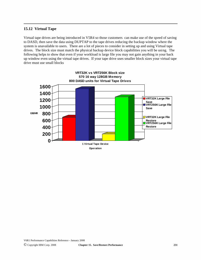
15.12 Virtual Tape

Virtual tape drives are being introduced in V5R4 so those customers can make use of the speed of savingto DASD, then save the data using DUPTAP to the tape drives reducing the backup window where thesystem is unavailable to users. There are a lot of pieces to consider in setting up and using Virtual tapedrives. The block size must match the physical backup device block capabilities you will be using. The following helps to show that even if your workload is large file you may not gain anything in your backup window even using the virtual tape drives. If your tape drive uses smaller block sizes your virtual tapedrive must use small blocks



0200400600800

1000120014001600

GB/HR

1 Virtual Tape DeviceOperation

VRT32K vs VRT256K Block size570 16 way 128GB Memory

800 DASD units for Virtual Tape Drives

VRT32K Large FileSaveVRT256K Large FileSave

VRT32K Large FileRestoreVRT256K Large FileRestore

The following measurements were done on a system with newer hardware including a 3580 Ultrium 34Gb Fiber Channel Tape Drive, 571E storage adapters, and 4327 70GB (U320) DASD.

Measurements were also done comparing save of 1000 empty libraries to tape versus save of theselibraries to virtual tape followed by DUPTAP from the virtual tape to tape. The save to tape was muchslower which can be explained as follows. When data is being saved to tape, a flush buffer is requestedafter each file is written to ensure that the file is actually on the tape. This forces the drive to backhitch foreach file and greatly reduces the performance. The DUPTAP command does not need to send a flushbuffer until the duplicate command completes, so it does not have the same performance impact.



0

0.5

1

1.5

2

2.5

3

3.5

4

Hou

rs to

Sav

e 1

TB o

f Dat

a

Larg

e Fi

leSa

ve to

Tap

e

Larg

e Fi

leSa

ve to

Virt

ual

Tape

then

DU

PTA

P

Use

r Mix

Sav

eto

Tap

e

Use

r Mix

Sav

eto

Virt

ual T

ape

then

DU

PTA

P

Save to Tape Vs. Save to Virtual Tape then DUPTAP to Tape570, 8 Way, 96GB Memory, 305 DASD units for Virtual Tape Drives

Restricted State Save to Tape Restricted State Save to Virtual Tape Non Restricted DUPTAP

0

10

20

30

Min

utes

to S

ave

Dat

a

Save to Tape Save to Virtual Tape then DUPTAP

Save to Tape Vs. Save to Virtual Tape then DUPTAP to Tape1000 Empty Libraries

3580 Ultrium 3 4Gb Fiber Tape Drive, 5761 4Gb Fiber Adapter571E Storage Adapters, 4327 70GB (U320) DASD

305 DASD units for Virtual Tape Drives570, 8 Way, 96GB Memory

Restricted State Save to Tape Restricted State Save to Virtual TapeNon Restricted DUPTAP

15.13 Parallel Virtual Tapes

NOTE: Virtual tape is reading and writing to the same DASD so the maximum throughput with ourconcurrent and parallel measurements is different than our tape drive tests where we were reading fromDASD and writing to tape.



0500

100015002000250030003500

GB/HR


Parallel Virtual Tape for Large File570 16 way 128GB Memory


1 Virtual Tape Device2 Virtual Tape Devices3 Virtual Tape Devices4 Virtual Tape Devices5 Virtual Tape Devices

0

50

100

150

200

250

300

GB/HR

Save Restore

Operation

Parallel Virtual Tape for User Mix570 16 way 128GB Memory



15.14 Concurrent Virtual Tapes

NOTE: Virtual tape is reading and writing to the same DASD so the maximum throughput with ourconcurrent and parallel measurements is different than our tape drive tests where we were reading fromDASD and writing to tape.



0500

100015002000250030003500

GB/HR


Concurrent Virtual Tape for Large File570 16 way 128GB Memory



0

200

400

600

800

1000

GB/HR

Save Restore

Operation

Concurrent Virtual Tape for User Mix570 16 way 128GB Memory



15.15 Save and Restore Scaling using a Virtual Tape Drive.

A 570 8 way System i was used for the following tests. A user ASP was created using up to 3 571FIOAs with up to 36 U320 70 GB DASD on each IOA. The Chart shows the number of DASD in each testand the Virtual tape drive was created using that DASD.

The workload data was restored into the system ASP and was then saved to the Virtual tape drive in theuser ASP. The system ASP consisted of 2 HSL loops, a mix of 571E and 571F IOAs and 312 - 70GBU320 DASD units. These charts are very specific to this DASD but the scaling flow would be similarwith different IOAs the actual rates would vary. For more information on the IOAs and DASD seeChapter 14 of this guide. Restoring the workloads from the Virtual tape drives started at 900 GB/HR reading from 6 DASD and scaled up to 1.5 TB/HR on the 108 DASD. The bottle neck will be limited towhere you are writing and how many DASD are available to the write operation.



Large File Virtual Tape Scaling(SAVE) Write to Virtual tape

0100200300400500600700800

6 DASD

12 D

ASD

18 D

ASD

24 D

ASD

30 D

ASD

36 D

ASD

42 D

ASD

48 D

ASD

54 D

ASD

60 D

ASD

66 D

ASD

72 D

ASD

78 D

ASD

84 D

ASD

90 D

ASD

96 D

ASD

102 D

ASD

108 D

ASD

GB

/HR

RAID5 SAVE RAID6 SAVE MIRRORING SAVE

User Mix Virtual Tape Scaling(SAVE) Write to Virtual Tape

050

100150200250300

6 DASD

12 D

ASD

18 D

ASD

24 D

ASD

30 D

ASD

36 D

ASD

42 D

ASD

48 D

ASD

54 D

ASD

60 D

ASD

66 D

ASD

72 D

ASD

78 D

ASD

84 D

ASD

90 D

ASD

96 D

ASD

102 D

ASD

108 D

ASD

GB

/HR


15.16 Save and Restore Scaling using 571E IOAs and U320 15K DASD units to a 3580Ultrium 3 Tape Drive.

A 570 8 way System i was used for the following tests. A user ASP was created with the number ofDASD listed in each test . The workload data was then saved to the tape drive , deleted from the systemand restored to the user ASP. These charts are very specific to the new IOAs and U320 capable DASDavailable. For more information on the IOAs and DASD see Chapter 14 of this guide.



Large File Save

0100200300400500600

6 DASD

12 D

ASD

18 D

ASD

24 D

ASD

30 D

ASD

36 D

ASD

42 D

ASD

48 D

ASD

54 D

ASD

60 D

ASD

66 D

ASD

72 D

ASD

78 D

ASD

84 D

ASD

90 D

ASD

GB

/HR


Large File Restore

0100200300400500600

6 DASD

12 D

ASD

18 D

ASD

24 D

ASD

30 D

ASD

36 D

ASD

42 D

ASD

48 D

ASD

54 D

ASD

60 D

ASD

66 D

ASD

72 D

ASD

78 D

ASD

84 D

ASD

90 D

ASD

GB/

HR

RAID5 RESTORE RAID6 RESTORE MIRRORING RESTORE



User Mix Saves

050

100150200250300350

6 DASD

12 D

ASD

18 D

ASD

24 D

ASD

30 D

ASD

36 D

ASD

42 D

ASD

48 D

ASD

54 D

ASD

60 D

ASD

66 D

ASD

72 D

ASD

78 D

ASD

84 D

ASD

90 D

ASD

GB/

HR


User Mix Restores

020406080

100120140160180

6 DASD

12 D

ASD

18 D

ASD

24 D

ASD

30 D

ASD

36 D

ASD

42 D

ASD

48 D

ASD

54 D

ASD

60 D

ASD

66 D

ASD

72 D

ASD

78 D

ASD

84 D

ASD

90 D

ASD

GB/

HR

RAID5 RESTORE RAID6 RESTORE MIRRORING RESTORE

15.17 High-End Tape Placement on System i

The current high-end tape drives (ULTRIUM-2 / ULTRIUM-3 and 3592-J / 3592-E) need to be placedcarefully on the System i buses and HSLs in order to avoid bottlenecking. The following rules-of thumbwill help optimize performance in a large-file save environment, and help position the customer for futuregrowth in tape activity:

vLimit the number of drives per fibre tape adapter as follows:For ULTRIUM-2, 3592-J, and slower drives, two drives can share a fc 5704 or fc 5761 fibre tape adapter.If running on a 2 GByte loop, a 3rd drive can share a fc 5761 fibre tape adapterFor ULTRIUM-3 and TS1120 (3592-E) drives, each drive should be on a separate fibre tape adapter

vPlace the fc 5704 or fc 5761 in a 64-bit slot on a “fast bus” as follows:PCI-X

In a 5094/5294 tower use slot C08 or C09.In a 5088/0588 tower use slot C08 or C09. You may need to purchase RPQ #847204 to allow the towerto connect with RIO-G performanceIn an 0595 or 5095 or 5790 expansion unit, use any valid slot

PCIIn a 5074/5079/5078 tower, use slot C02, C03 or C04

Note“Ensure the fc 5761 is supported on your CPU type”

vPut one fc 5704 or fc 5761 per tower initially. On loops running at 2 GByte speeds, a second fc 5704 card can beadded according to the locations recommended above if needed.

vSpread tape fibre cards across as many HSL’s as possible, with maximums as followOn Loops running at 1 GByte (e.g. all loops on 8xx systems, or loops with HSL-1 towers )

Maximum of two drives per HSL loopOn Loops running at 2 GByte (eg loops with all HSL-2 / RIO-G towers on system i systems)

Maximum of six ULTRIUM-2 or 3592-J drives per RIO-G loop. Maximum of four ULTRIUM-3 drives or TS1120 (3592-E) drives per RIO-G loop using the fc5704 IOA. Maximum of two TS1120 (3592-E) drives per RIO-G loop using the fc 5761 IOA

v If Gbit Ethernet cards are present on the system and will be running during the backups, then treat them as thoughthey were ULTRIUM-3 or TS1120 (3592-E) tape drives when designing the card and HSL placement using therules above since they can command similar bandwidth

The rules above assume that the customer is running a large-file workload and that all tape drives are activesimultaneously. If your customer is running a user-mix tape workload or the high load cards are not runningsimultaneously, then it may be possible to put more gear on the bus/HSL than shown. There may also be certaincard layouts that will allow more drives per bus/tower/HSL, but these need to be reviewed individually.



15.18 BRMS-Based Save/Restore Software Encryption and DASD-Based ASP Encryption

The Ultrium-3 was used in the following experiments, which attempt to characterize the effects ofBRMS-based save /restore software encryption and DASD-based ASP encryption. Some of the newertape drives offer hardware encryption as an option but for those who are not looking to upgrade or investin these tape units at this time, software encryption can be a fair solution. In the experiments we used fullprocessors that were dedicated to the partition. We used a 9406-MMA 4 way partition and a 9406-570 4way partition. Both systems had 40 GB of main memory. The workload data was located on a singleuser ASP with 36 - 70GB 15K RPM DASD attached through a 571F IOA. The experiments were not setup to show the best possible environment or to take into account all of the possible hardwareenvironments, instead these experiments were an attempt to portray some of the differences customersmight observe if they choose software encryption as a back up strategy over their current non-encryptedenvironment. Software encryption has a significant impact on save times but only a minor impact torestore times



Tape Backup Performance - Saves

0100200300400500600700

1 GB Source File 12 GB User Mix 64 GB Large File 320 GB Large File

GB/

HR

9406-MMA-4w ay Encrypted ASP SAVLIBBRM NO Softw are Encryption9406-MMA-4w ay Encrypted ASP SAVLIBBRM With Softw are Encryption9406-MMA-4w ay NON Encrypted ASP SAVLIBBRM NO Softw are Encryption9406-MMA-4w ay NON Encrypted ASP SAVLIBBRM With Softw are Encryption9406-570-4w ay NON Encrypted ASP SAVLIBBRM NO Softw are Encryption9406-570-4w ay NON Encrypted ASP SAVLIBBRM With Softw are Encryption

CPU Utilization during Saves

05

10152025


%CP

U Us

ed

9406-MMA-4w ay %CPU Used Encrypted ASP SAVLIBBRM NO Softw are Encryption9406-MMA-4w ay %CPU Used Encrypted ASP SAVLIBBRM With Softw are Encryption9406-MMA-4w ay %CPU Used NON Encrypted ASP SAVLIBBRM NO Softw are Encryption9406-MMA-4w ay %CPU Used NON Encrypted ASP SAVLIBBRM With Softw are Encryption9406-570-4w ay %CPU Used NON Encrypted ASP SAVLIBBRM NO Softw are Encryption9406-570-4w ay %CPU Used NON Encrypted ASP SAVLIBBRM With Softw are Encryption

Performance will be limited to the native drive rates (shown in table 15.1.1) because encrypted datablocks have a very low compaction ratio.



Tape Backup Performance - Restores

050

100150200250300


GB/

HR

9406-MMA-4w ay Encrypted ASP RSTLIBBRM NO Softw are Encryption9406-MMA-4w ay Encrypted ASP RSTLIBBRM With Softw are Encryption9406-MMA-4w ay NON Encrypted ASP RSTLIBBRM NO Softw are Encryption9406-MMA-4w ay NON Encrypted ASP RSTLIBBRM With Softw are Encryption9406-570-4w ay NON Encrypted ASP RSTLIBBRM NO Softw are Encryption9406-570-4w ay NON Encrypted ASP RSTLIBBRM With Softw are Encryption

CPU Utilization during Restores

0

5

10

15

20


%C

PU U

sed

9406-MMA-4w ay %CPU Used Encrypted ASP RSTLIBBRM NO Softw are Encryption9406-MMA-4w ay %CPU Used Encrypted ASP RSTLIBBRM With Softw are Encryption9406-MMA-4w ay %CPU Used NON Encrypted ASP RSTLIBBRM NO Softw are Encryption9406-MMA-4w ay %CPU Used NON Encrypted ASP RSTLIBBRM With Softw are Encryption9406-570-4w ay %CPU Used NON Encrypted ASP RSTLIBBRM NO Softw are Encryption9406-570-4w ay %CPU Used NON Encrypted ASP RSTLIBBRM With Softw are Encryption

15.19 5XX Tape Device RatesNote: Measurements for the high speed devices were completed on a 570 4 way system with 2844 IOPsand 2780 IOA’s and 180 15K RPM RAID5 DASD units. The smaller tape device tests were completedon a 520 2 way with 75 DASD units. The Virtual tape and *SAVF runs were completed on a 570 ML16with 256GB of memory and 924 DASD units. The goal of each of the tests is to show the capabilities ofthe device and so a system large enough to achieve the maximum throughput for that device was used.Customer performance will be dependent on over all systems resources and if those resources match themaximum capabilities of the device. See other sections in this guide about memory, CPU and DASD.

1100105049038038026020014056403434R1100110050038035023020012570403434S

Network Storage Space

1200100056050042023019011055332929R1250100053050041023019012567352929S

Domino Mail Files

3023303030992320999R555050505050503540302525SMany Directories

Many Objects

605060605016144730131312R706565656565653540272523S1 Directory

Many Objects

15301340830570510R

17001420890580525SLarge File 320GB

1500134083056050039033017568R

1450133083056050036535022582SLarge File 64GB

8005605003903301756840R8005605003653502258241S

Large File 32GB

340280373432R280280373432S

Large File 4GB

180125180180150120809653353130R22022021021020018015014570403532S

User Mix 12GB

1155048333130R13011348333130SUser Mix 3GB

202030302920202419191719R353530302217172119141717S

Source File 1GB

V5R4V5R3V5R4V5R4V5R4V5R3V5R3V5R4V5R4V5R3V5R4V5R4Release Measurements were done

Virtual Tape D

rive

*SAV

F

3592E Fiberfc 5761 4G

B Fiber A

dapter

3592E Fiber5704 2G

B Fiber A

dapter

3580 Ultrium

35704 2G

B Fiber A

dapter

3592J5704 2G

B Fiber A

dapter

3580 Ultrium

25704 2G

B Fiber A

dapter

5755½

High U

LTRIU

M 2

6279 VX

A-320

VX

A-2

SLR100

SLR60

WorkloadS = Save

R = Restore

Table 15.19.1 Measurements in (GB/HR) Workload data Saved and Restored from User ASP 2.



3419R3419S


2915R2915S

Domino Mail Files


Many Objects

128R2312S1 Directory

Many Objects

3237R

3239SLarge File 32GB

3030R3034S

User Mix 12GB

1915R1722S

Source File 1GB

V5R4V5R4M0Release Measurements were done

SLR60 from

table 15.18.1

6258 4MM

tape Drive

WorkloadS = Save

R = Restore

Table 15.19.2 - V5R4M0 Measurements on an 5XX 1-way system 8 RAID5 protected DASD Units 8 GB memoryMeasurements in (GB/HR) all 8 DASD in the system ASP .



15.20 5XX Tape Device Rates with 571E & 571F Storage IOAs and 4327 (U320) Disk Units

Save/restore rates of 3580 Ultrium 3 (2Gb and 4Gb Fiber Channel) tape devices and of virtual tapedevices were measured on a 570 8-way system with 571E and 571F storage adapters and 714 type 432770GB (U320) disk units. Customer performance will be dependent on overall system resources and howwell those resources match the maximum capabilities of the device. See other sections in this guide aboutmemory, CPU and DASD.

1230525460405380R1300425410355350S


1190600460460420R1410550450440410S

Domino Mail Files


Many Objects

6545606050R8090808065S1 Directory

Many Objects

1240760785550510R

1420650635525525SLarge File 320GB

1230760785550500R

1380650585510500SLarge File 64GB

195182175175150R345295290290200S

User Mix 12GB

4026404029R110551109522S

Source File 1GB

V5R4V5R4V5R4V5R4V5R4Release Measurements were done

Virtual Tape D

rive

3580 Ultrium

4 5761 4G

b Fiber Adapter

3580 Ultrium

35761 4G

b Fiber Adapter

3580 Ultrium

35704 2G

b Fiber Adapter

3580 Ultrium

35704 2G

b Fiber Adapter

571E/571F Storage IOAs4327 70GB (U320) DASD

2780 StorageIOAs

4326 35GB(U160) DASD

(Data from table15.18.1)

WorkloadS = Save

R = Restore

Table 15.20.1 Measurements in (GB/HR)

Workload data Saved and Restored from User ASP 2.



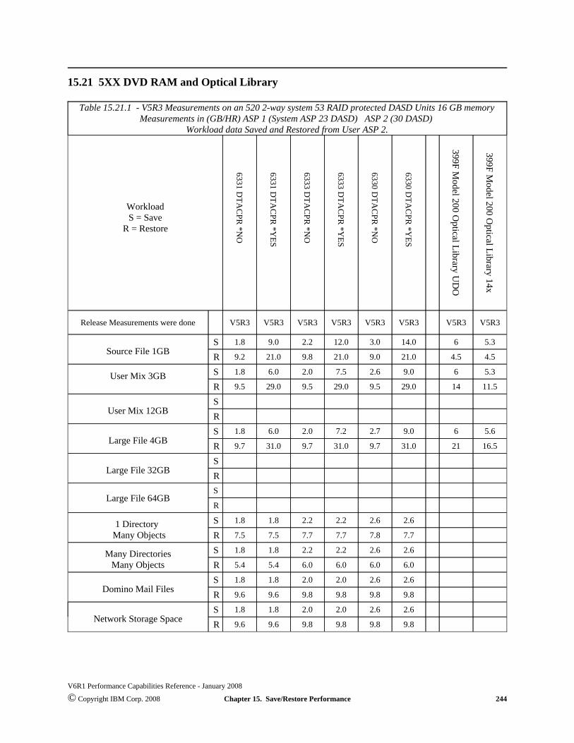
15.21 5XX DVD RAM and Optical Library

9.89.89.89.89.69.6R2.62.62.02.01.81.8S


9.89.89.89.89.69.6R2.62.62.02.01.81.8S

Domino Mail Files

6.06.06.06.05.45.4R2.62.62.22.21.81.8SMany Directories

Many Objects

7.77.87.77.77.57.5R2.62.62.22.21.81.8S1 Directory

Many Objects

R

SLarge File 64GB

RS

Large File 32GB

16.52131.09.731.09.731.09.7R5.669.02.77.22.06.01.8S

Large File 4GB

RS

User Mix 12GB

11.51429.09.529.09.529.09.5R5.369.02.67.52.06.01.8SUser Mix 3GB

4.54.521.09.021.09.821.09.2R5.3614.03.012.02.29.01.8S

Source File 1GB

V5R3V5R3V5R3V5R3V5R3V5R3V5R3V5R3Release Measurements were done

399F Model 200 O

ptical Library 14x

399F Model 200 O

ptical Library UD

O

6330 DTA

CPR

*YES

6330 DTA

CPR

*NO

6333 DTA

CPR

*YES

6333 DTA

CPR

*NO

6331 DTA

CPR

*YES

6331 DTA

CPR

*NO

WorkloadS = Save

R = Restore

Table 15.21.1 - V5R3 Measurements on an 520 2-way system 53 RAID protected DASD Units 16 GB memoryMeasurements in (GB/HR) ASP 1 (System ASP 23 DASD) ASP 2 (30 DASD)

Workload data Saved and Restored from User ASP 2.



15.22 Software CompressionThe rates a customer will achieve will depend upon the system resources available. This test was run in avery favorable environment to try to achieve the maximum rates. Software compression rates weregathered using the QSRSAVO API. The CPU used in all compression schemes was near 100%. Thecompression algorithm cannot span CPUs so the fact that measurements were performed on a 24-waysystem doesn’t affect the software compression scenario.

6539Restore3:166SaveV5R2 Using

API DTACPR*HIGH

3123Restore2.7:12726SaveV5R2 Using

API DTACPR*MED

5737Restore1.5:110888SaveV5R2 Using

API DTACPR*LOW

480507Restore48020019SaveV5R2170457Restore17013519SaveV5R1

SoftwareCompression

RatioSR16GBNUMX12GBNSRC1GB

Table 15.22.1 - Measurements on an 840 24-way system 1080 RAID protected DASD Units (GB/HR) 128 GBmainstore



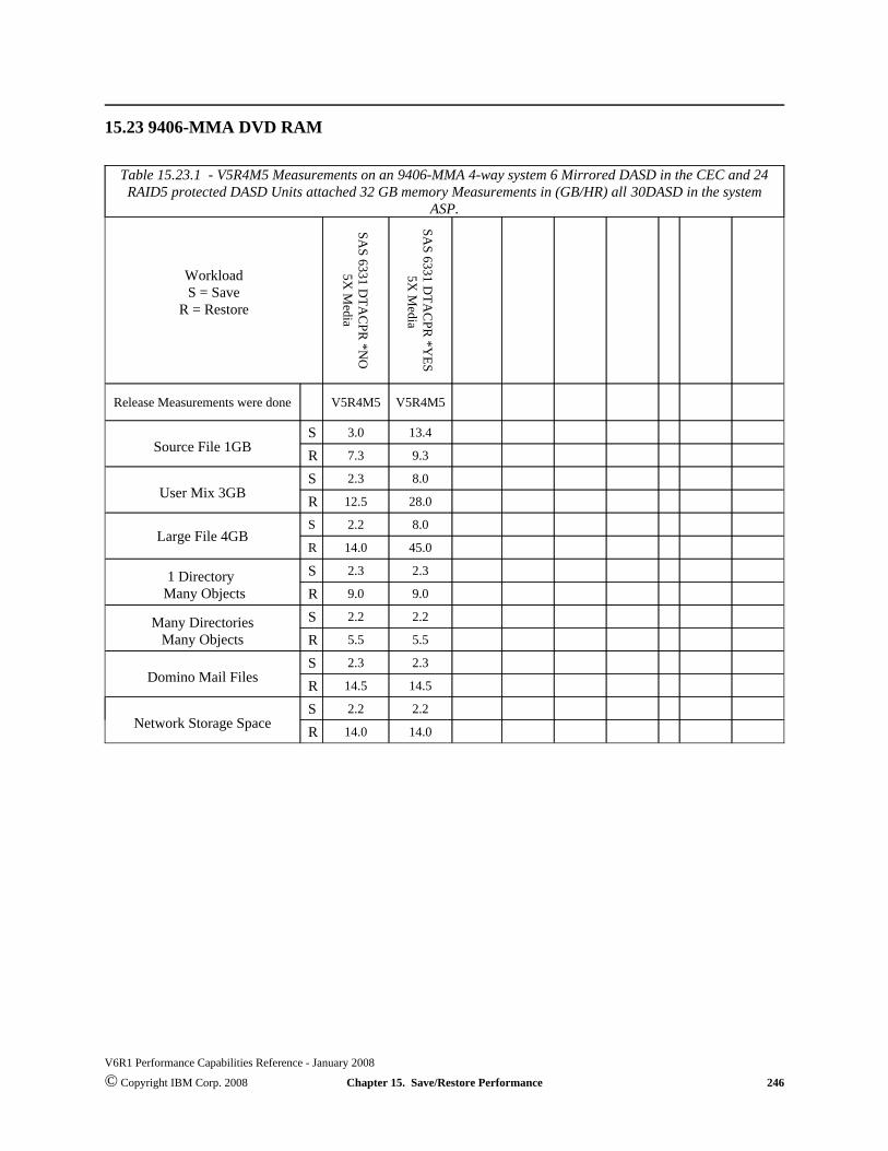
15.23 9406-MMA DVD RAM

14.014.0R2.22.2S


14.514.5R2.32.3S

Domino Mail Files

5.55.5R2.22.2SMany Directories

Many Objects

9.09.0R2.32.3S1 Directory

Many Objects

45.014.0R

8.02.2SLarge File 4GB

28.012.5R8.02.3S

User Mix 3GB

9.37.3R13.43.0S

Source File 1GB

V5R4M5V5R4M5Release Measurements were done

SAS 6331 D

TAC

PR *Y

ES 5X

Media

SAS 6331 D

TAC

PR *N

O5X

Media

WorkloadS = Save

R = Restore

Table 15.23.1 - V5R4M5 Measurements on an 9406-MMA 4-way system 6 Mirrored DASD in the CEC and 24RAID5 protected DASD Units attached 32 GB memory Measurements in (GB/HR) all 30DASD in the system

ASP.



15.24 9406-MMA 576B IOPLess IOA

700700580450R700330500450S

Domino Mail Files


Many Objects

50505050R50505050S1 Directory

Many Objects

770750845590R


770750810590R


220220230190R280220230280S

User Mix 12GB

42424545R40402740S

Source File 1GB

V6R1M0V6R1M0V6R1M0V6R1M0Release Measurements weredone

Virtual Tape

120 DA

SD in A

SP2

Virtual Tape

60 DA

SD in A

SP2

3592E Fiber576B

2 Port 4G

b Fiber Adapter

3580 Ultrium

3576B

2 Port 4G

b Fiber Adapter

WorkloadS = Save

R = Restore

Table 15.24.1 - V6R1M0 Measurements on an 9406-MMA 4-way system 145 RAID5 protected DASD Units inthe system ASP, attached via 571F IOAs 40 GB memory Measurements in (GB/HR).Two different Virtual tape experiments with 60 DASD ASP2 and 120 DASD in ASP2



15.25 What’s New and Tips on Performance

What’s New

V6R1M0March 2008BRMS-Based Save/Restore Software Encryption and DASD-Based ASP Encryption576B IOPLess Storage IOA

V5R4M5 July 20073580 Ultrium 4 - 4Gb Fiber Channel Tape Drive6331 SAS DVD RAM for 9406-MMA system models

V5R4January 2007 571E and 571F storage IOAs (see DASD Performance chapter for more information)

August 20061. DUPTAP performance PTFs (V5R4 - SI23903, MF39598, MF39600, and MF39601) 2. 3580 Ultrium 3 4Gb Fiber Channel Tape Drive

January 20061. Virtual Tape2. Parallel IFS3. 3580 Ultrium 3 2Gb Fiber Channel Tape Drive4. 3592E 5. VXA-3206. ½ High Ultrium 27. IFS Restore Improvements for the Directory Workloads8. 5761 4Gb Fiber Adapter

TIPS

1. Backup devices are affected by the media type. For most backup devices the right media and densitycan greatly affect the capacity and speed of your save or restore operation. USE THE RIGHTMEDIA FOR YOUR BACKUP DEVICE. (i.e. Use a 25 GB tape cartridge in a 25 GB drive).

2. A Backup and Recovery Management System such as BRMS/400 is recommended to keep track ofthe data and make the most of multiple backup devices.

3. Domino Online Performance Tips:Http://www-03.ibm.com/servers/eserver/iseries/service/brms/domperftune.html



Http://www-03.ibm.com/servers/eserver/iseries/service/brms/domperftune.html

Chapter 16 IPL Performance Performance information for Initial Program Load (IPL) is included in this section.

The primary focus of this section is to present observations from IPL tests on different System i models.The data for both normal and abnormal IPLs are broken down into phases, making it easier to see the detail. For information on previous models see a prior Performance Capabilities Reference.

NOTE: The information that follows is based on performance measurements and analysis done in theServer Group Division laboratory. Actual performance may vary significantly from these tests.

16.1 IPL Performance Considerations

The wide variety of hardware configurations and software environments available make it difficult tocharacterize a 'typical' IPL environment and predict the results. The following section provides a simpledescription of the IPL tests.

16.2 IPL Test Description

Normal IPL Power On IPL (cold start after managed system was powered down completely)For a normal IPL, benchmark time is measured from power-on until the System i server consolesign-on screen is available.

Abnormal IPLSystem abnormally terminated causing recovery processing to be done during the IPL. Theamount of processing is determined by the system activities at the time the system terminates. For an abnormal IPL, the benchmark consists of bringing up a database workload and letting itrun until the desired number of jobs are running on the system. Once the workload is stabilized,the system is forced to terminate, forcing a mainstore dump (MSD). The dump is then copied toDASD via the Auto Copy function. The Auto Copy function is enabled through System ServiceTools (SST). The System i partition is set to normal so that once the dump is copied, the systemcompletes the remaining IPL with no user intervention. Benchmark time is measured from thetime the system is forced to terminate, to when the System i server console sign on screen isavailable.Settings: on the CHGIPLA command the parameter, HDWDIAG, set to (*MIN). All physicalfiles are explicitly journaled. Also logical files are journaled using SMAPP (System ManagedAccess Path Protection) by using the EDTRCYAP command set to *MIN.

NOTE: Due to some longer starting tasks ( like TCP/IP ), all workstations may not be up and ready at thesame time as the console workstation displays a sign-on screen.


© Copyright IBM Corp. 2008 Chapter 16 IPL Performance 249

16.3 9406-MMA System Hardware Information

16.3.1 Small system Hardware Configuration 9406-MMA 7051 4 way - 32 GB Mainstore DASD / 30 70GB 15K rpm arms, 6 DASD in CEC Mirrored 24 DASD in a #5786 EXP24 Disk Drawer attached with a 571F IOA RAID5 Protected

Software Configuration 100,000 spool files (100,000 completed jobs with 1 spool file per job) 500 jobs in job queues (inactive) 600 active jobs in system during Mainstore dump 1000 user profiles, 1000 libraries Active Database: 2 libraries with 500 physical files and 20 logical files

16.3.2 Large system Hardware Configurations 9406-MMA 7056 8 way - 96 GB Mainstore DASD / 432 70GB 15K rpm arms, 3 ASP's defined, 108 RAID5 DASD in ASP1, 288 RAID5 DASD in ASP2, 36 DASD no protection in ASP3 - Mainstore dump set to ASP 2

This system was tested with database files unrelated to this test covering 30% of the DASD space available, this database load causes a long directory recovery.

9406-MMA 7061 16 way - 512 GB Mainstore DASD / 1000 70GB 15K rpm arms, 3 ASP's defined, 196 Nonconfigured DASD, 120 RAID5 DASD in ASP1, 612 RAID5 DASD in ASP2, 72 DASD no protection in ASP3 - Mainstore dump set to ASP 2

This system was tested with database files unrelated to this test covering 30% of the DASD space available, this database load causes a long directory recovery.

Software Configuration400,000 spool files (400,000 completed jobs with 1 spool files each)1000 jobs waiting on job queues (inactive)11000 active jobs in system during mainstore dump200 remote printers, 6000 user profiles, 6000 librariesActive Database:

25 libraries with 2600 physical files and 452 logical files2 libraries with 10,000 physical files and 200 logical files

NOTE:Physical files are explicitly journaledLogical files are journaled using SMAPP set to *MINCommitment Control used on 20% of the files



16.4 9406-MMA IPL Performance Measurements (Normal)

The following tables provide a comparison summary of the measured performance data for a normal and abnormal IPL. Results provided do not represent any particular customer environment.

Measurement units are in minutes and seconds

34:2732:0317:58 9:428:47 Total2:222:412:12 1:23:48 OS/4009:5810:057:53 5:074:49 SLIC

22:0719:177:533:123:10 Hardware

V6R1GA3 Firmware

16 Way9406-MMA

7061512 GB

1000 DASD

V5R4M5 GA1 Firmware

16 Way9406-MMA

7061512 GB

1000 DASD

V5R4M5GA1 Firmware

8 Way9406-MMA

705696 GB

432 DASD

V6R1GA3 Firmware

4 Way9406-MMA

705132 GB

30 DASD

V5R4M5 GA1 Firmware

4 Way 9406-MMA

7051 32 GB

30 DASD

Table 16.4.1 V5R4M5 Normal IPL - Power-On (Cold Start)

Generally, the hardware phase is composed of C1xx xxxx, C3xx xxxx and C7xx xxxx. SLIC iscomposed of C200 xxxx and C600 xxxx. OS/400 is composed of C900 xxxx SRCs to the System i serverconsole sign-on.

16.5 9406-MMA IPL Performance Measurements (Abnormal)

Measurement units are in minutes and seconds.

42:4952:0045:0820:4418:44 Total20:4729:2728:065:044:22 OS/400

3:284:022:321:293:09 SLICre-ipl

3:042:283:182:242:00 Shutdown re-ipl

10:5611:357:0010:457:23 SLIC MSDIPL

with Copy

4:344:284:121:021:50 ProcessorMSD

V6R1 GA3 Firmware

16 Way9406-MMA

7061512 GB

1000 DASD

V5R4M5 GA1 Firmware

16 Way9406-MMA

7061512 GB

1000 DASD

V5R4M5GA1 Firmware

8 Way9406-MMA

705696 GB

432 DASD

V6R1GA3 Firmware

4 Way9406-MMA

705132 GB

30 DASD

V5R4M5 GA1 Firmware

4 Way 9406-MMA

7051 32 GB

30 DASD

Table 16.5.1 V5R4M5 Abnormal IPL (Partition MSD)



16.6 NOTES on MSD

MSD is Mainstore Dump. General IPL phase as it relates to the SRCs posted on the operation panel: Processor MSD includes the D2xx xxxx and C2xx xxxx right after the system is forced to terminate.SLIC MSD IPL with Copy follows with the next series of C6xx xxxx, see the next heading for moreinformation on the SLIC MSD IPL with Copy. The copy occurs during the C6xx 4404 SRCs. Shutdownincludes the Dxxx xxxx SRCs. Hardware re-ipl includes the next phase of D2xx xxxx and C2xx xxxx.SLIC re-IPL follows which are the C600 xxxx SRCs. OS/400 completes with the C900 xxxx SRCs.

16.6.1 MSD Affects on IPL Performance Measurements

SLIC MSD IPL with Copy is affected by the number of DASD units and the jobs executing at the time ofthe mainstore dump.

When a system is abnormally terminated, in-process changes to the directories used by the system tomanage storage may be lost. During the subsequent IPL, storage management directory recovery isperformed to ensure the integrity of the directories and the underlying storage allocations.

The duration of this recovery step will depend on the type of recovery performed and on the size of thedirectories. In most cases, a subset directory recovery (SRC C6004250) will be performed which maytypically run from 2 minutes to 30 minutes depending upon the system. In rare cases, a full directoryrecovery (SRC C6004260) is performed which typically runs much longer than a subset directoryrecovery. The duration of the subset directory recovery is dependent on the size of the directory (whichrelates to the amount of data stored on the system) and on the amount of in-process changes. With theamount of data stored on our largest configurations with one to two thousand disk units, subset directoryrecovery (SRC C6004250) took from 14 minutes to 50 minutes depending upon the system.

DASD Unit’s Effect on MSD Time - Through experimental testing we found the time spent in MSDcopying the data to disk is related to the number of DASD arms available. Assigning the MSD copy to anASP with a larger number of DASD can help reduce your recovery time if an MSD should occur.



16.7 5XX System Hardware Information

16.7.1 5XX Small system Hardware Configuration

520 7457 2 way - 16 GB MainstoreDASD / 23 35GB 15K rpm arms,RAID Protected

Software Configuration100,000 spool files (100,000 completed jobs with 1 spool file per job)500 jobs in job queues (inactive)500 active jobs in system during Mainstore dump1000 user profiles1000 libraries

Database:2 libraries with 500 physical files and 20 logical files

16.7.2 5XX Large system Hardware Configuration

570 7476 16 way - 256 GB MainstoreDASD / 924 35GB arms 15K rpm arms,RAID protected, 3 ASP's defined, majority of the DASD in ASP2 - Mainstore dump was to ASP 2

This system was tested with 2 TB of database files unrelated to this test, but this load causes a longdirectory recovery.

595 7499 32-way - 384 GB MainstoreDASD / 1125 35GB arms 15K rpm armsRAID protected, 3 ASP's defined, majority of the DASD in ASP2 - Mainstore dump was to ASP 2

This system was tested with 4 TB of database files unrelated to this test, but this load causes a longdirectory recovery.

Software Configuration400,000 spool files (400,000 completed jobs with 1 spool files each)1000 jobs waiting on job queues (inactive)11000 active jobs in system during mainstore dump200 remote printers6000 user profiles6000 libraries

Database:25 libraries with 2600 physical files and 452 logical files2 libraries with 10,000 physical files and 200 logical files

NOTE:Physical files are explicitly journaledLogical files are journaled using SMAPP set to *MINCommitment Control used on 20% of the files



16.8 5XX IPL Performance Measurements (Normal)

The following tables provide a comparison summary of the measured performance data for a normal andabnormal IPL. Results provided do not represent any particular customer environment.

Measurement units are in minutes and seconds

The workloads were increased for V5R4 to better reflect common system load affecting the OS/400 portion of the IPL 39:4637:1026:5926:518:5010:08Total3:432:302:321:32:501:00OS/4009:368:506:436:424:303:49SLIC26:2725:5017:4418:373:305:19Hardware

V5R4GA7 Firmware

32 Way5957499

384 GB1125 DASD

V5R3GA3 Firmware

32 Way595

7499384 GB MS1125 DASD

V5R4 GA7 Firmware

16 Way570

7476256 GB

924 DASD

V5R3 GA3 Firmware

16 Way570

7476256 GB

924 DASD

V5R4GA7 Firmware

2 Way5207457

16 GB23 DASD

V5R3GA3 Firmware

2 Way5207457

16 GB23 DASD

Table 16.8.1 Normal IPL - Power-On (Cold Start)

Generally, the hardware phase is composed of C1xx xxxx, C3xx xxxx and C7xx xxxx on the 5xxsystems. SLIC is composed of C200 xxxx and C600 xxxx. OS/400 is composed of C900 xxxx SRCs tothe System i5 server console sign-on.

16.9 5XX IPL Performance Measurements (Abnormal)

Measurement units are in hours, minutes and seconds.

The workloads were increased for V5R4 to better reflect common system load affecting the MSD and the OS/400 portion of theIPL

1:40:371:08:021:22:2744:1730:0113:31Total44:1013:5625:4509:564:2003:21OS/400

6:2104:165:2203:592:1701:59SLICre-ipl

3:5703:592:2304:192:5002:46Shutdown re-ipl

40:0343:1042:1824:1015:4004:50SLIC MSDIPL

with Copy

6:0602:416:3901:534:5400:35ProcessorMSD

V5R4GA7 Firmware

32 Way5957499

384 GB1125 DASD

V5R3GA3 Firmware

32 Way595

7499384 GB MS1125 DASD

V5R4GA7 Firmware

16 Way5707476

256 GB 924 DASD

V5R3 GA3 Firmware

16 Way570

7476256 GB

924 DASD

V5R4GA7 Firmware

2 Way5207457

16 GB23 DASD

V5R3GA3 Firmware

2 Way520

745716 GB

23 DASD

Table 16.9.1 Abnormal IPL (Partition MSD)



16.10 5XX IOP vs IOPLess effects on IPL Performance (Normal)

Measurement units are in minutes and seconds.

28:1826:59Total2:522:32OS/4007:206:43SLIC

18:0617:44Hardware

V5R4 GA7 Firmware

16 Way IOPLess5707476

256 GB 924 DASD

V5R4 GA7 Firmware

16 Way IOP5707476

256 GB924 DASD

Table 16.10.2 Normal IPL - Power-On (Cold Start)

16.11 IPL Tips

Although IPL duration is highly dependent on hardware and software configuration, there are tasks thatcan be performed to reduce the amount of time required for the system to perform an IPL. The followingis a partial list of recommendations for IPL performance:

Remove unnecessary spool files. Use the Display Job Tables (DSPJOBTBL) command to monitorthe size of the job table(s) on the system. Change IPL Attributes (CHGIPLA) command can be usedto compress job tables if there is a large number of available job table entries. The IPL to compressthe tables maybe longer, so try to plan it along with a normal maintenance IPL where you have thetime to wait for the table to compress.

Reduce the number of device descriptions by removing any obsolete device descriptions.

Control the level of hardware diagnostics by setting the CHGIPLA command to specifyHDWDIAG(*MIN), the system will perform only a minimum, critical set of hardware diagnostics.This type of IPL is appropriate in most cases. The exceptions include a suspected hardware problem,or when new hardware, such as additional memory, is being introduced to the system.

Reduce the amount of rebuild time for access paths during an IPL by using System Managed AccessPath Protection (SMAPP). The System i5 Backup and Recovery book (SC41-5304) describes thismethod for protecting access paths from long recovery times during an IPL.

For additional information on how to improve IPL performance, refer to System i5 Basic SystemOperation, Administration, and Problem Handling (SC41-5206) - or to the redbook The SystemAdministrator’s Companion to System i5 Availability and Recovery (SG24-2161).



Chapter 17. Integrated BladeCenter and System x Performance

This chapter provides a performance overview and recommendations for the Integrated xSeries Server4, theIntegrated xSeries Adapter and the iSCSI host bus adapter. In addition, the chapter presents some performancecharacteristics and impacts of these solutions on System i™.

17.1 Introduction

The Internet SCSI Host Bus Adapter (iSCSI HBA), the Integrated xSeries® Server for iSeries™ (IXS),and the Integrated xSeries Adapter (IXA) extend the utility of the System i solution by integrating x86and AMD based servers with the System i platform. Selected models of Intel based servers may runWindows® 2000 Server editions, Windows Server 2003 editions, Red Hat® Enterprise Linux®, orSUSE® LINUX Enterprise Server. In addition, the iSCSI HBA allows System i models to integrate andcontrol IBM System x and IBM BladeCenter® model servers. For more information about supported models, operating systems, and options, please see the “System iintegration with BladeCenter and System x” web page referenced at the end of this chapter. Also, see theiSeries Information Center content titled “Integrated operating environments - Windows environment oniSeries” for iSCSI and IXS/IXA concepts and operation details.In the text following, the System i platform is often referred to as the “host” server. The IXS, IXAattached server, or the iSCSI HBA attached server is referred to as the “guest” server.V5R4 iSCSI Host Bus Adapter (iSCSI HBA)

The iSCSI host bus adapters (hardware type #573B Copper and #573C Fiber-optic) have been introducedin V5R4. The iSCSI HBA supports 1Gbit Ethernet network connections, and provides i5/OS systemmanagement and disk consolidation for guest System x and BladeCenter platforms.

The iSCSI HBA solution provides an extensive scalability range - from connecting up to 8 guest serversthrough one iSCSI HBA for a lower cost connectivity, to allowing up to 4 iSCSI HBAs per individualguest server for scalable bandwidth. For information about the numbers of supported adapters please seethe “System i integration with BladeCenter and System x” web page.

With the iSCSI HBA solution, no disks are installed on the guest servers. The host i5/OS server providesdisks, storage consolidation, guest server management, along with the tape, optical, and virtual ethernetdevices. Currently, only Windows 2003 Server editions, with SP1 or release 2, are supported with theiSCSI solution.

The Integrated xSeries Adapter (IXA)

The Integrated xSeries Adapter (IXA - hardware type #2689-001 or #2689-002) is a PCI-based interfacecard that installs inside selected models of System x, providing a High Speed Link (HSL) connection to ahost i5/OS system. The guest server provides the processors, memory, and Server Proven adapters, but nodisks5. IXA attached SMP servers support larger workloads, more users and greater flexibility to attachdevices than the IXS uni-processor models.

V6R1 Performance Capabilities Reference - January 2008 © Copyright IBM Corp. 2008 Chapter 17 - Integrated BladeCenter and System x Performance 256

5 With the IXA - all the disk drives used by the guest server are under the control of the host server. The are nodisk drives in the guest server.

4 The IBM System i and IBM System x product family names have replaced the IBM eSeries iSeries and xSeriesproduct family names. However, the IXS and IXA adapters retain the iSeries and xSeries brand labels.

Integrated xSeries Servers (IXS)

An Integrated xSeries Server is an Intel processor-based server on a PCI-based interface card that plugsinto a host system. This card provides the processor, memory, USB interfaces, and in some cases, abuilt-in gigabit Ethernet adapter. There are several hardware versions of the IXS:

The 2.0 GHz Pentium® M IXS (hardware type #4812-001)6.The 2.0 GHz PCI IXS (hardware type #2892-002).

Older versions of the IXS Card are: the 1.6 GHz PCI IXS (hardware type #2892-001), 1 GHz (type#2890-003), 850 Mhz (type #2890-002), and 700 MHz (type #2890-001).

17.2 Effects of Windows and Linux loads on the host system

The impact of IXS and IXA device I/O operations on the host system is similar for all versions of the IXAand IXS cards. The IXA and IXS cards and drivers channel the host directed device I/O through an Input /Output processor (IOP) on the card..

The iSCSI HBA is an IOP-less input/output adapter. The internal operation and performancecharacteristics differ from the IXS/IXA solutions - with a slightly higher host CPU, and memoryrequirements. However, the iSCSI solution offers greater scalability and overall improved performancecompared to the IXS/IXA. The iSCSI solution adds support for IBM BladeCenter and additional Systemx models.

Depending on the Windows or Linux application activity, integrated guest server I/O operations imposean indirect load on the System i native CPU, memory and storage subsystems. The rest of this chapterdescribes some of the performance and memory resource impacts.

17.2.1 IXS/IXA Disk I/O Operations:The integrated xSeries servers use i5/OS network server storage spaces for its hard drives, which areallocated out of i5/OS storage. For the IXS/IXA server - IBM supplied virtual SCSI drivers render these storage spaces as physical disksin Windows or Linux. The device drivers cooperate with i5/OS to perform the disk operations, andadditional host CPU resource is used during disk access, along with a fixed amount of storage. Theamount of CPU impact is a function of the disk I/O rate and disk operation size.The disk linkage type and Windows driver write cache property alters the CPU cost and average writelatency.

Fixed and Dynamically Linked Disks

Fixed (statically) and dynamically linked disk drives have the same performance characteristics. Oneadvantage of dynamically linked drives is that in most cases, they may be linked and unlinked whilethe server is active.

Shared Disks

System i Windows integration supports the Microsoft Clustering Service, which supports “shared”disks. When a storage space is linked as a “shared” disk, all write operations require extendedcommunications to insure data integrity, which slightly increases the host CPU cost and responsetime.


6 Requires a separate IOP card, which is included with features 4811, 4812 and 4813.

Write Cache Property

When the disk device write cache property is disabled, disk operations have similar performancecharacteristics to shared disks. You may examine or change the “Write Cache” property on Windowsby selecting disk “properties” and then the “Hardware tab”. Then view “Properties” for a selecteddisk and view the “Disk Properties” or “Device Options” tab.

All dynamically and statically linked storage spaces have “Write Cache” enabled by default. Sharedlinks have “Write Cache” disabled by default. While it is possible to enable “Write Cache” on shareddisks, we recommend to keep it disabled to insure integrity during clustering fail-over operations.There is also negligible performance benefit to enabling the write cache on shared disks.

Extended Write OperationsEven though a Windows disk driver may have write cache enabled, the system or applicationsconsider some write operations sensitive enough to request extended writes or flush operations “writethrough” to the disk. These operations incur the higher CPW cost regardless of the write cachingproperty.For the IXS and IXA solutions - do not enable the disk driver “Enable advanced performance”property provided in Windows 2003. When enabled, all extended writes are turned into normalcached operations and flush operations are masked. This option is only intended to be used when theintegrity of the write operations can be guaranteed via write through or battery backed memory. TheIXS/IXA with write caching enabled cannot make this guarantee.IXS/IXA Disk Capacity ConsiderationsThe level of disk I/O achieved on the IXS or IXA varies depending on many variables, but given anadequate storage subsystem, the upper cap on I/O for a single server is limited by the IXS/IXA IOPcomponent. Except in extreme test loads, it’s unlikely the IOP will saturate due to disk activity.When multiple IXS/IXA servers are attached under the same System i partition, the partition softwareimposes a cap on the aggregate total I/O from all the servers. It is not a strict limitation, but a typicalcapacity level is approximately 6000 to 10000 disk operations/sec.

17.2.2 iSCSI Disk I/O Operations:The iSCSI disk operations use a more scalable storage I/O access architecture than the IXS and IXAsolutions. As a result, a single integrated server can scale to greater capacity by using multiple targetand initiator iSCSI HBAs to allow multiple data paths. In addition, there is no inherent partition cap to the iSCSI disk I/O. The entire performance capacityof installed disks and disk IOAs is available to iSCSI attached servers.

• The Windows disk drive “write cache” policy does not directly affect iSCSI operations. Writeoperations always “write through” to the host disk IOAs, which may or may not cache in batterybacked memory (depending on the capabilities and configuration of the disk IOA).iSCSI attached servers use non-reserved System i virtual storage in order to perform disk input oroutput. Thus, disk operations use host memory as an intermediate read cache. Write operations areflushed to disk immediately, but the disk data remains in memory and can be read on subsequentoperations to the same sectors.While the disk operations page through a memory pool, the paging activity is not visible in the “Non-DB”pages counters displayable via the WRKSYSSTS command. This doesn’t mean the memory is notactively used, it’s just difficult to visualize how much memory is active. WRKSYSSTS will show faultsand paging activity if the memory pool becomes constrained, but some write operations also result infaulting activity.


With iSCSI, there are some Windows side disk configuration rules you must take into account toenable efficient disk operations. Windows disks should be configured as:

1 disk partition per virtual drive.File system formatted with cluster sizes of 4 kbyte or 4 kbyte multiples. 2 gigabyte or larger storage spaces (for which Windows creates a default NTFS cluster size of4kbytes).

If necessary, you can use care to configure multiple disk partitions on a single virtual drive.For storage spaces that are 1024 MB or less, make the partitions a multiple of 1 MB (1,048,576bytes).For storage spaces that are 511000 MB or less, the partition should be a multiple of 63 MB(66060288 bytes).For storage spaces that are greater than 511000 MB, the partition should be a multiple of 252 MB(264,241,152 bytes).

These guidelines allow file system structures to align efficiently between iSCSI Windows/Linux andi5/OS7. They allow i5/OS to efficiently manage the storage space memory, mitigate disk operationfaulting activity, and thus improve overall iSCSI disk I/O performance. Failure to follow theseguidelines will cause iSCSI disk write operations to incur performance penalties, including pagefaults and increased serialization of disk operations.In V5R4 – the CHGNWSSTG command and iSeries Navigator now supports the expansion of a storagespace size. After the expansion, the file system in the disk should also be expanded - but take care oniSCSI disks: don’t create a new partition in the expanded disk free space (unless the new partitionsmeeting the size guidelines above).

The Windows 2003 “DISKPART” command can be used to perform the file system expansion – howeverit only actually expands the file system on “basic” disks. If a disk has been converted to a “dynamic”disk8, the DISKPART command creates a new partition and configures a spanned set across the partitions.With iSCSI, the second partition may experience degraded disk performance.

17.2.3 iSCSI virtual I/O private memory pool

Applications sharing the same memory pool with iSCSI disk operations may be adversely impacted if theiSCSI network servers perform levels of disk I/O which can flush the memory pool. Thus, it is possiblefor other applications to begin to page fault because their memory has been flushed out to disk by theiSCSI operations. By default, the iSCSI virtual disk I/O operations occur through the *BASE memorypool. In order to segregate iSCSI disk activity, V5R4 PTF SI23027 has been created to enable iSCSI virtualdisk I/O operations to run out of an allocated private memory pool. The pool is enabled by creating asubsystem description named QGPL/QFPHIS and allocating a private memory pool of at least 4096kilobytes. The amount of memory you want to allocate will depend on a number of factors, includingnumber of iSCSI network servers, expected sustained disk activity for all servers, etc. See the “System iMemory Rules of Thumb” section below for more guidelines on the “iSCSI private pool” minimum size.To activate the private memory pool for all iSCSI network servers, perform the following:

1. CRTSBSD SBSD(QGPL/QFPHIS) POOLS((1 10000 1))9


9 Pick a larger or smaller pool size as appropriate. 10,000 KByte is a reasonable minimum value, but 4096 KByteis the absolute minimum supported.

8 Not to be confused with “dynamically linked” storage spaces.

7 These guidelines could also slightly improve IXS and IXA attached servers’ disk performance, but to a muchsmaller degree.

2. Vary on any Network Server Description (NWSD) with a Network server connection type of *ISCSI.During the iSCSI network server vary on processing the QFPHIS subsystem is automatically started ifnecessary. The subsystem will activate the private memory pool. iSCSI network server descriptions thatare varied on will then utilize the first private memory pool configured with at least the minimum (4MB)size for virtual disk I/O operations. The private memory pool is used by the server as long as the subsystem remains active. If the QFPHISsubsystem is ended prematurely (while an iSCSI network server is active), the server will continue tofunction properly but future virtual disk I/O operations will revert to the *BASE memory pool until thesystem memory pool is once again allocated. NOTE: When ending the QFPHIS subsystem, i5/OS can reallocate the memory pool, possibly assigningthe same identifier to another subsystem! Any active iSCSI network servers that are varied on and usingthe memory pool at the time the subsystem is ended may adversely impact other applications either whenthe memory pool reverts to *BASE or when the memory pool identifier is reassigned to anothersubsystem! To prevent unexpected impacts – do not end the QFPHIS subsystem while iSCSI servers areactive.

17.2.4 Virtual Ethernet Connections: The virtual Ethernet connections utilize the System i systems licensed internal code tasks duringoperation. When a virtual Ethernet port is used to communicate between Integrated servers, or betweenservers across i5/OS partitions, the host server CPU is used during the transfer. The amount of CPU usedis primarily a function of the number of transactions and their size. There are three forms of Virtual Ethernet connections used with the IXS/IXA and iSCSI attached servers:

The “Point to point virtual Ethernet” is primarily used for the controlling partition to communicatewith the integrated server. This network is called point to point because it has only two endpoints, theintegrated server and the i5/OS platform. It is emulated within the host platform and no additionalphysical network adapters or cables are used. In host models, it is configured as an Ethernet linedescription with Port Number value *VRTETHPTP.

A “Port-based”10 virtual Ethernet connection allows IXS, IXA or iSCSI attached servers tocommunicate together over a virtual Ethernet (typically used for clustered IXS configurations), or tojoin an inter-LPAR virtual Ethernet available on non-POWER5 based systems This type of virtualEthernet uses “network numbers”, and integrated servers can participate by configuring a port numbervalue in the range *VRTETH0 through *VRTETH9.

“Port-based” virtual Ethernet communications also require the host CPU to switch thecommunications data between guest servers.

A “VLAN-based” (noted as Phyp in charts) virtual Ethernet connection allows IXS, IXA and iSCSIattached servers to participate in inter-LPAR virtual Ethernets. Each participating integrated serverneeds an Ethernet line description that associates a port value such as *VRTETH0 with a virtualadapter having a virtual LAN ID. You create the virtual adapter via the Hardware ManagementConsole (HMC).

VLAN-based communications also use the System i CPU to switch the communications data betweenserver.

17.2.5 IXS/IXA IOP Resource:


10“Port-Based” refers to the original method of supporting VE introduced in V5R2 for models earlier than Systemi5. It is still available for integrated servers to communicate within a single partition on System i models.

IXS and IXA I/O operations (disk, tape, optical and virtual Ethernet) communications occur through theindividual IXS and IXA IOP resource. This IOP imposes a finite capacity. The IOP processor utilizationmay be examined via the iSeries Collection Services utilities.

The performance results presented in the rest of this chapter are based on measurements andprojections using standard IBM benchmarks in a controlled environment. The actual throughputor performance that any user will experience will vary depending upon considerations such as theamount of multiprogramming in the user's job stream, the I/O configuration, the storageconfiguration, and the workload processed. Therefore, no assurance can be given that anindividual user will achieve throughput or performance improvements equivalent to the ratiosstated here.

17.3 System i memory rules of thumb for IXS/IXA and iSCSI attached servers.

The i5/OS machine pool memory “rule of thumb” is generally to size the machine pool with at least twicethe active machine pool reserved size. Automatic performance adjustments may alter this according to theactive load characteristics. But, there are base memory requirements needed to support the hardware andset of adapters used by the i5/OS partition. You can refer to the System i sales manual or Work LoadEstimator for estimates of these base requirements. The “rules of thumb” below estimates the additionalmemory required to support iSCSI and IXS/IXA.

17.3.1 IXS and IXA attached servers:I/O occurs through fixed memory in the machine pool. The IXS and IXA attached servers requireapproximately an additional 4MBytes of memory per server in the machine pool.

17.3.2 iSCSI attached servers:IBM Director Server is required in each i5/OS partition running iSCSI HBA targets. IBM Directorrequires a minimum of 500 Mbytes in the base pool.The specific memory requirements of iSCSI servers vary based on many configuration choices, includingthe number of LUNs, number of iSCSI target HBAs, number of NWSDs, etc. A suggested minimummemory “rule of thumb”11 is:


11Based on a rough configuration of 5 LUNS per server, 2 VE connections per server, and two target HBAconnections per server.

2.5 MBytes22.5 MBytesTotal:

1 MByte120.5 MByteQFPHIS Private Pool:

0.5 MByte1 MByteBase Pool:

1 MByte21 MBytes Machine Pool:

For Each NWSDFor Each Target HBA

Warning: To ensure expected performance and continuing machine operation, it is critical toallocate sufficient memory to support all of the devices that are varied on. Inadequate memorypools can cause unexpected machine operation.

17.4 Disk I/O CPU Cost

155IXS/IXA shared or quorum linked disks or write cachingdisabled

130IXS/IXA static or dynamically linked disks with write cachingenabled

190iSCSI linked disks

CPWs13 / 1k ops/secDisk Operation Rules of Thumb

While the disk I/O activity driven by the IXS/IXA or iSCSI is not strictly a “CPW” type load, the CPWestimate is still a useful metric to estimate the amount of i5/OS CPU required for a load. You can use thevalues above to estimate the CPW requirements if you know the expected I/O rate. For example, if youexpect the Windows application server to generate 800 disk ops/sec on a dynamically or statically linkedstorage space, you can estimate the CPW usage as:

130 cpws/1kops * 800ops * 1kops/1000ops = 130 * 800/1000 = 104 CPWs out of the host processor CPW capacity. While it is always better to project the performance of anapplication from measurements based on that same application, it is not always possible. This calculationtechnique gives a relative estimate of performance.These rules of thumb are estimated from the results of performing file serving or application types ofloads. In more detail, the chart below indicates an approximate amount of host processor (in CPW)required to perform a constant number of disk operations (1000) of various sizes. You can reasonablyadjust this estimate linearly for your expected I/O level.


13A CPW is the “Relative System Performance Metric” from Appendix C. Note that the I/O CPU capacities maynot scale exactly by rated system CPW, as the disk I/O doesn’t represent a CPW type of load . This calculation isa convenient metric to size the load impacts. The measured CPW cost will actually decrease from the abovevalues as the number of processors in the NWSD hosting partition increases, and may be higher than estimatedwhen partial processors are used.

12Private pool assigned to QFPAIS must still be a 4 MB minimum size.

CPW per 1k Disk Operations

0

100

200

300

400

500

60051

2 W

rite

1k W

rite

2k W

rite

4k W

rite

8k W

rite

16k

Writ

e24

k W

rite

32k

Writ

e64

k W

rite

512

Rea

d1k

Rea

d2k

Rea

d4k

Rea

d8k

Rea

d16

k R

ead

24k

Rea

d32

k R

ead

64k

Rea

d

512

RW

1k R

W2k

RW

4k R

W8k

RW

16k

RW

24k

RW

32k

RW

64k

RW

File

Ser

v

AppS

erv

CPW

/ 1k

Ops

/sec

iSCSI IXS/IXA w Caching Disabled or Shared IXS/IXA w Caching Enabled

The charts shows the relative cost when performing 5 different types of operations14. Random write operations of a uniform size (512, 1k, ... 64k).Random read operations of a uniform size (512, 1k, ... 64k). A 35% random write, 65% random read mix of operations with a uniform size (termed transactionprocessing type load).A fileserving type load - which consists of a mix of operations of various sizes similar in ratio totypical fileserving loads. This load is 80% random reads. An application server - database type load. This is also a mix to simulate the character of applicationand database type accesses - mostly random with about 40% reads.

17.4.1 Further notes about IXS/IXA Disk OperationsMaximum disk operation size supported by the IXS or IXA is 32k. Thus, any Windows diskoperations greater than 32k will result in the Windows operating system splitting the operation into 2or more sequential operations. The IXS/IXA cost calculation is slightly greater on a POWER5® system (System i5) than on earlier8xx systems. This includes some increased overhead costs in V5R4, and the new processor types. Usethe newer rules of thumb listed above for CPW calculations.It does not matter if a storage space is linked statically or dynamically, the performancecharacteristics are identical. It does not matter if a server is an IXS or an IXA attached System x server, the disk performance isalmost identical.


14Measured on a System i Model 570 - 2-way 26F2 processor (7495 capacity card), rated at 6350 CPWs, V5R4release of i5/OS, 40 parity protected (RAID 5) 4326 disks, 3 2780 disk controllers. The IXA attached server wasa x365xSeries (4way 2.5Ghz Xeon with IXA and Windows Server 2003 with SP1. The iSCSI servers were HS20BladeCenter servers with a copper iSCSI (p/n 26K6489) daughter card. Switches were Nortel L2/3 Ethernet (p/n26K6524) and Cisco Intelligent Gigabit Switch (p/n )

A storage space which is linked as shared, or a disk with caching disabled, requires more CPU toprocess write operations (approx. 45%). Sequential operations cost approximately 10% less than the random I/O results shown above.Even though a Windows disk driver may have write cache enabled, some Windows applications mayrequest to bypass the cache for some operations (extended writes), and these operations would incurthe higher CPW cost.If your application load is skewed to the upper or lower average disk operations, you may encounter asmaller or larger CPW cost than indicated by the “rules of thumb”.

17.5 Disk I/O Throughput

The chart below compares the throughput performance characteristics of the current IXA product againstthe new iSCSI solution. The charts indicates an approximate capacity of a single target HBA whenrunning various sizes and types of random operations. The chart below also demonstrates that the new page based architecture utilized in the iSCSI solutionprovides better over all performance in Write and Read scenarios. While the sector based architecture ofthe current IXA provides slightly better performance in small block Write operations, that difference isquickly reversed when block sizes reach 4k. 4k block sizes and higher are representative of more I/Oserver scenarios.As with all performance analysis, the actual values that you will achieve are dependent on a number ofvariables including workload, network traffic, etc..

iSCSI Target, IXA Capacity ComparisonMB per Second

020406080

100120140160

512

Ran

dWrit

e1k

Ran

dWrit

e2k

Ran

dWrit

e4k

Ran

dWrit

e8k

Ran

dWrit

e16

k R

andW

rite

24k

Ran

dWrit

e32

k R

andW

rite

64k

Ran

dWrit

e12

8k R

andW

rite

512

Ran

dRea

d1k

Ran

dRea

d2k

Ran

dRea

d4k

Ran

dRea

d8k

Ran

dRea

d16

k R

andR

ead

24k

Ran

dRea

d32

k R

andR

ead

64k

Ran

dRea

d12

8k R

andR

ead

512

Ran

dRW

1k R

andR

W2k

Ran

dRW

4k R

andR

W8k

Ran

dRW

16k

Ran

dRW

24k

Ran

dRW

32k

Ran

dRW

64k

Ran

dRW

128k

Ran

dRW

MB

/sec

IXA iSCSI 1 Targ 1 Init StdiSCSI 1 Targ 4 Init Std iSCSI 1 Targ 4 Init Jumbo


The blue square line shows an iSCSI connection with a single target iSCSI HBA - single initiator iSCSIHBA connection, configured to run with standard frames. The pink circle line is a single target iSCSIHBA to multiple servers and initiators running also running with standard frames. With the initiators andswitches configured to use 9k jumbo frames, a 15% to 20% increase in upper capacity is demonstrated.15

17.6 Virtual Ethernet CPU Cost and Capacities

If the virtual Ethernet connections are used for any significant LAN traffic, you need to account foradditional System i CPU requirements. There is no single rule of thumb applicable to network traffics, asthere are a great number of variables involved. The charts below demonstrate approximate capacity for single TCP/IP connections, and illustrates theminimum CPW impacts for some network transaction sizes (send/receive operations) and types gatheredwith the Netperf 16exerciser. The CPW chart below gives CPWs per Mbit/sec for increasing transactionsizes. When the transaction size is small, the CPW requirements are greater per transaction. When thearrival rate is high enough, some consolidation of operations within the process stream can occur andincrease efficiency of operations. Several charts are presented comparing the virtual ethernet capacity and costs between an iSCSI serverrunning jumbo frames and standard frames, and a IXS or IXA server. In addition, a comparison of costswhile using external NICs is added, to place the measurements in context. The “Point-to-Point” refers tothe cost between an iSCSI, IXS or IXA attached server and an host system across the point to pointconnection. “Port Based VE” refers to a port-based connection between two guest servers in the samepartition. “VLAN based VE” refers to a Virtual LAN based connection between two guest servers in thesame partition, but using the VLAN to port associated virtual adapters. In the latter two cases, the totalCPW cost would be split across partitions if the communication would occur between guest servershosted by different partitions17.

17.6.1 VE Capacity ComparisonsIn general, VE has less capacity than an external Gigabit NIC. Greater capacity with VE is possible using9k jumbo frames than with using standard 1.5k frames. Also, the iSCSI connection has a greater capacity


17Netperf TCP_STREAM measured on a System i Model 570 - 2-way 26F2 processor (7495 capacity card), rated at6350 CPWs, V5R4 release of i5/OS. The IXA attached server was a x365xSeries (4way 2.5Ghz Xeon with IXAand Windows Server 2003 with SP1. The iSCSI servers were HS20 BladeCenter 32.Ghz uniprocessor serverswith a copper iSCSI (p/n 26K6489) daughter card. Switches were Nortel L2/3 Ethernet (p/n 26K6524). This isonly a rough indicator for capacity planning, actual results may differ for other hardware configurations.

16Note that the Netperf benchmark consists of C programs which use a socket connection to read and write databetween buffers. The CPW results above don’t attempt to factor out the minimal application CPU cost. That is,the CPW results above include the primitive Netperf application, socket, TCP, and Ethernet operation costs. Areal user application will only have this type of processing as a percentage of the overall workload.

15In addition, jumbo frame configuration has no effect on the CPW cost of iSCSI disk operations.

than an IXS or IXA attached VE connection. “Stream” means that the data is pushed in one direction,with only the TCP acknowledge packets running in the other direction.

17.6.2 VE CPW Cost CPW cost below is listed as CPW per Mbit/sec. For the point to point connection, the results are differentdepending on the direction of transfer. For connections between guest servers - the direction of transferdoesn’t matter to the results.


PP TCP Stream i5/OS to Windows

0100200300400500600700800900

1000

16 32 64 128

256

512

1024

2048

4096

8192

1638

432

768

Transaction Size (bytes)

Thro

ughp

ut (M

Bits

/sec

)

iscsi jumboiscsi standardIXS/IXAexternal NICs

PP TCP Stream Windows to i5/OS

0100200300400500600700800900

1000

16 32 64 128

256

512

1024

2048

4096

8192

1638

432

768


Thro

ughp

ut (M

Bits

/sec

)


VE Internal (port based)

0100200300400500600700800900

1000

16 64 256 1024 4096 16384Transaction Size (bytes)

Thro

ughp

ut (M

Bits

/sec

)


VEPhyp Stream TCP

0100200300400500600700800900

1000

16 64 256 1024 4096 16384Transaction Size (bytes)

Thro

ughp

ut (M

Bits

/sec

)iscsi jumboiscsi standardIXS/IXAexternal NICs

PP TCP Stream i5/OS to Windows

0.0

5.0

10.0

15.0

20.0

25.0

128

256

512

1024

2048

4096

8192

1638

432

768


CPW

per

MB

its/s

ec


PP TCP Stream Windows to i5/OS

0.05.0

10.015.020.025.030.035.040.0

128

256

512

1024

2048

4096

8192

1638

432

768


CPW

per

MB

its/s

ec

iscsi jumboiscsi standardIXS/IXAexternal NICsVE Internal (port based)

02

46

810

1214

16

128

256

512

1024

2048

4096

8192

1638

432

768


CPW

per

MB

its/s

ec

iscsi jumboiscsi standardIXS/IXA

VEPhyp Stream TCP

0

5

10

15

20

25

128

256

512

1024

2048

4096

8192

1638

432

768


CPW

per

MB

its/s

ec

iscsi jumboiscsi standardIXS/IXA

The chart above shows the CPW efficiency of operations (larger is better). Note the CPW per Mbits/secscale on the left - as it’s different for each chart. For an IXS or IXA, the port-based VE has the least CPW or smaller packets due to consolidation oftransfers available in Licensed Internal Code. The VLAN-based transfers have the greatest cost (Howeverthe total would be split during inter-LPAR communications).For iSCSI, the cost of using standard frames is 1.5 to 4.5 times higher than jumbo frames. 17.6.3 Windows CPU CostThe next chart illustrates the cost of iSCSI port-based, and VLAN-based virtual ethernet operations on awindows CPU. In this case, the CPUs used are 3.2Ghz Xeon uniprocessor between HS20 BladeCenterservers. This cost is compared to operations across the external gigabit NIC connections. Again, thejumbo frames operations are less expensive than standard frames, though the external NIC is twice asefficient in General.

Streaming TCP Total Windows CPU Util

0.000.100.200.300.400.500.600.700.800.901.00

128

256

512

1024

2048

4096

8192

1638

432

768


Tota

l CPU

Util

per

MB

its/s

ec External - Window s to Window s (std)External - Window s to Window s (jumbo)Port Based VE - Window s to Window s (std)Port Based VE - Window s to Window s (jumbo)Vlan Based VE - Window s to Window s (std)Vlan Based VE - Window s to Window s (jumbo)

17.7 File Level Backup Performance

The Integrated Server support allows you to save integrated server data (files, directories, shares, and theWindows registry) to tape, optical or disk (*SAVF) in conjunction with your other i5/OS data. That is,this “file level backup” approach saves or restores the Windows files on an individual basis within thestream of other i5/OS data objects. It’s not recommended that this approach is used as a primary backupprocedure. Rather, you should still periodically save your NWS storage spaces and the NWSD associatedwith your Windows server or Linux server for disaster recovery.

Saving individual files does not operate as fast as saving the individual storage spaces. The save of astorage space on a equivalent machine and tape is about 210 Gbytes per hour, compared to theapproximately 70 Gbytes per hour achieved using iSCSI below.

The chart below compares some SAV and RST rates for iSCSI and an IXA attached server. These resultswere measured on a System i Model 570 2-way 26F2 processor (7495 capacity card). The i5/OS releasewas V5R4. The IXA attached comparison server was an x365 xSeries (4way 2.5Ghz Xeon with IXA andWindows Server 2003 with SP1). The iSCSI servers were HS20 BladeCenter servers with a copperiSCSI (p/n 26K6489) daughter card. Switches were Nortel L2/3 Ethernet (p/n 26K6524). The target tapedrive was a model 5755-001 (Ultrium LTO 2). All tests were run with jumbo frames enabled.


The legend label “Mixed Files” indicates a save of many files of mixed sizes - equivalent to the save ofthe Windows system file disk. “Large files” indicates a save of many large files - in this case many100MB files.

FLBU SAV / RST Rates

0.00

10.00

20.00

30.00

40.00

50.00

60.00

70.00

80.00

90.00

SAV to disk SAV to Tape RST from disk RST from Tape

GB

per

Hr

iSCSI Large iSCSI Mixed IXA Large IXA Mixed

17.8 Summary

The iSCSI host bus adapter, Integrated xSeries Server and Integrated xSeries Adapter provides scalableintegration for full file, print and application servers running Windows 2000 Server, Windows Server2003 or with Intel Linux editions. They provide flexible consolidation of System i solutions andWindows or Linux services, in combination with improved hardware control, availability, and reducedmaintenance costs. These solutions perform well as a file or application server for popular applications,using the System i host disks, tape and optical resources. The iSCSI HBA addition in V5R4 increasesIntegrated server configuration flexibility and performance scalability. As part of the preparation forintegrated server installations, care should be taken to estimate the expected workload of the Windows orLinux server applications and reserve sufficient i5/OS resources for the integrated servers.

17.9 Additional Sources of Information

System i integration with BladeCenter and System x URL: http://www.ibm.com/systems/i/bladecenter/

Redbook: “Microsoft Windows Server 2003 Integration with iSeries”, SG246959 at http://www.redbooks.ibm.com/abstracts/SG246959.html

Redbook: “Tuning IBM eServer xSeries Servers for Performance SG24-5287”http://www.redbooks.ibm.com/abstracts/sg245287.html While this document doesn’t address the integrated server configurations specifically, it is anexcellent resource for understanding and addressing performance issues with Windows or Linux.

Online documentation: “Integrated operating environments on iSeries”http://publib.boulder.ibm.com/iseries/


http://www.ibm.com/systems/i/bladecenter/

http://www.redbooks.ibm.com/abstracts/SG246959.html

http://www.redbooks.ibm.com/abstracts/sg245287.html

http://publib.boulder.ibm.com/iseries/

Choose V5R4. In the “Contents” panel choose “iSeries Information Center”.Expand “Integrated operating environments” and then “Windows environment on iSeries” forWindows environment information or “Linux” and then “Linux on an integrated xSeries solutionfor Linux Information on an IXS or attached xSeries server.

Microsoft Hardware Compatibility Test URL: See http://www.microsoft.com/whdc/hcl/search.mspx search on IBM for product types Storage/SCSI Controller and System/Server Uniprocessor.


http://www.microsoft.com/whdc/hcl/search.mspx

Chapter 18. Logical Partitioning (LPAR)

18.1 Introduction

Logical partitioning (LPAR) is a mode of machine operation where multiple copies of operating systemsrun on a single physical machine.

A logical partition is a collection of machine resources that are capable of running an operating system. The resources include processors (and associated caches), main storage, and I/O devices. Partitionsoperate independently and are logically isolated from other partitions. Communication between partitionsis achieved through I/O operations.

The primary partition provides functions on which all other partitions are dependent. Any partition thatis not a primary partition is a secondary partition. A secondary partition can perform an IPL, can bepowered off, can dump main storage, and can have PTFs applied independently of the other partitions onthe physical machine. The primary partition may affect the secondary partitions when activities occur thatcause the primary partition’s operation to end. An example is when the PWRDWNSYS command is runon a primary partition. Without the primary partition’s continued operation all secondary partitions areended.

V5R3 Information

Please refer to the whitepaper ‘i5/OS LPAR Performance on POWER4 and POWER5 Systems’ for thelatest information on LPAR performance. It is located at the following website:

http://www-1.ibm.com/servers/eserver/iseries/perfmgmt/pdf/lparperf.pdf

V5R2 Additions

In V5R2, some significant items may affect one's LPAR strategy (see "General Tips"):

"Zero" interactive partitions. You do not have to allocate a minimum amount of interactiveperformance to every partition when V5R2 OS is in the Primary partition.

In V5R2, the customer no longer has to assign a minimum interactive percentage to LPAR partitions (canbe 0). For partitions with no assigned interactive capability, LPAR system code will allow interactive asfollows: 0.1% x (processors in partition/total processors) x processor CPW.

In V5R1, the customer had to allocate a minimum interactive percentage to LPAR partitions as follows: 1.5% x (processors in partition/total processors) x processor CPW. It is expected that the LPARsystem code will issue a PTF to change the percentage from 1.5% to 0.5% for V5R1 systems. Notes: 1. The above formulas yield the minimum ICPW for an LPAR region. The customer still has to divide this value bythe total ICPW to get the percentage value to specify for the LPAR partition. 2. If there is not enough interactive CPW available for the partition given the previous formula ... the interactivepercentage can be set to the percentage of the (processors in partition/total processors).

General Tips


© Copyright IBM Corp. 2008 Chapter 18 - LPAR 270

http://www-1.ibm.com/servers/eserver/iseries/perfmgmt/pdf/lparperf.pdf

Allocate fractional CPUs wisely. If your sizing indicates two partitions need 0.7 and 0.4 CPUs, see ifthere will be enough remaining capacity in one of the partitions with 0.6 and 0.4 or else 0.7 and 0.3CPUs allocated. By adding fractional CPUs up to a "whole" processor, fewer physical processorswill be used. Design implies that some performance will be gained.Avoid shared processors on large partitions if possible. Since there is a penalty for having sharedprocessors (see later discussion), decide if this is really needed. On a 32 way machine, a wholeprocessor is only about 3 per cent of the configuration. On a 24 way, this is about 4 per cent. Thoughwe haven't measured this, the general penalty for invoking shared processors (often, five per cent)means that rounding up to whole processors may actually gain performance on large machines.

V5R1 Additions

In V5R1, LPAR provides additional support that includes: dynamic movement of resources without asystem or partition reset, processor sharing, and creating a partition using Operations Navigator. For moreinformation on these enhancements, click on System Management at URL: http://submit.boulder.ibm.com/pubs/html/as400/bld/v5r1/ic2924/index.htm

With processor sharing, processors no longer have to be dedicated to logical partitions. Instead, a sharedprocessor pool can be defined which will facilitate sharing whole or partial processors among partitions.There is an additional system overhead of approximately 5% (CPU processing) to use processor sharing.

Uniprocessor Shared Processors. You can now LPAR a single processor and allocate as little as 0.1CPUs to a partition. This may be particularly useful for Linux (see Linux chapter).

18.2 ConsiderationsThis section provides some guidelines to be used when sizing partitions versus stand-alone systems. Theactual results measured on a partitioned system will vary greatly with the workloads used, relative sizes,and how each partition is utilized. For information about CPW values, refer to Appendix D, “CPW, CIWand MCU Values for iSeries”.

When comparing the performance of a standalone system against a single logical partition with similarmachine resources, do not expect them to have identical performance values as there is LPAR overheadincurred in managing each partition. For example, consider the measurements we ran on a 4-way systemusing the standard AS/400 Commercial Processing Workload (CPW) as shown in the chart below.

For the standalone 4-way system we used we measured a CPW value of 1950. We then partitioned thestandalone 4-way system into two 2-way partitions. When we added up the partitioned 2-way values asshown below we got a total CPW value of 2044. This is a 5% increase from our measured standalone4-way CPW value of 1950. I.e. (2044-1950)/1950 = 5 %. The reason for this increased capacity can beattributed primarily to a reduction in the contention for operating system resources that exist on thestandalone 4-way system.

Separately, when you compare the CPW values of a standalone 2-way system to one of the partitions (i.e.one of the two 2-ways), you can get a feel for the LPAR overhead cost. Our test measurement showed acapacity degradation of 3%. That is, two standalone 2-ways have a combined CPW value of 2100. Thetotal CPW values of two 2-ways running on a partitioned four way, as shown above, is 2044. I.e.(2100-2044)/2044 = -3%.



http://submit.boulder.ibm.com/pubs/html/as400/bld/v5r1/ic2924/index.htm

The reasons for the LPAR overhead can be attributed to contention for the shared memory bus on apartitioned system, to the aggregate bandwidth of the standalone systems being greater than thebandwidth of the partitioned system, and to a lower number of system resources configured for a systempartition than on a standalone system. For example on a standalone 2-way system the main memoryavailable may be X, and on a partitioned system the amount of main storage available for the 2-waypartition is X-2.

LPAR Performance Considerations

1019 10501950

1025 1050

S/Alone 4-W LPAR 2/2 W 2 x 2-W0

500

1000

1500

2000

2500

Th

rou

ghp

ut

in C

PW

5% increase 3% decrease

Figure 18.1. LPAR Performance Measured Against Standalone Systems

In summary, the measurements on the 4-way system indicate that when a workload can be logically splitbetween two systems, using LPAR to configure two systems will result in system capacities that aregreater than when the two applications are run on a single system, and somewhat less than splitting theapplications to run on two physically separate systems. The amount of these differences will varydepending on the size of the system and the nature of the application.

18.3 Performance on a 12-way system

As the machine size increases we have seen an increase in both the performance of a partitioned systemand in the LPAR overhead on the partitioned system. As shown below you will notice that the capacityincrease and LPAR overhead is greater on a 12-way system than what was shown above on a 4-waysystem.



Also note that part of the performance increase of an larger system may have come about because of areduction in contention within the CPW workload itself. That is, the measurement of the standalone12-way system required a larger number of users to drive the system’s CPU to 70 percent than what isrequired on a 4-way system. The larger number of users may have increased the CPW workload’sinternal contention. With a lower number of users required to drive the system’s CPU to 70 percent on astandalone 4-way system., there is less opportunity for the workload’s internal contention to be a factor inthe measurements.

The overall performance of a large system depends greatly on the workload and how well the workloadscales to the large system. The overall performance of a large partitioned system is far more complicatedbecause the workload of each partition must be considered as well as how each workload scales to thesize of the partition and the resources allocated to the partition in which it is running. While the partitionsin a system do not contend for the same main storage, processor, or I/O resources, they all use the samemain storage bus to access their data. The total contention on the bus affects the performance of eachpartition, but the degree of impact to each partition depends on its size and workload.

In order to develop guidelines for partitioned systems, the standard AS/400 Commercial ProcessingWorkload (CPW) was run in several environments to better understand two things. First, how does thesum of the capacity of each partition in a system compare to the capacity of that system running as asingle image? This is to show the cost of consolidating systems. Second, how does the capacity of apartition compare to that of an equivalently sized stand-alone system?

The experiments were run on a 12-way 740 model with sufficient main storage and DASD arms so thatCPU utilization was the key resource. The following data points were collected:

Stand-alone CPW runs of a 4-way, 6-way, 8-way, and 12-wayTotal CPW capacity of a system partitioned into an 8-way and a 4-way partitionTotal CPW capacity of a system partitioned into two 6-way partitionsTotal CPW capacity of a system partitioned into three 4-way partitions

The total CPW capacity of a partitioned system is greater than the CPW capacity of the stand-alone12-way, but the percentage increase is inversely proportional to the size of the largest partition. The CPWworkload does not scale linearly with the number of processors. The larger the number of processors, thecloser the contention on the main storage bus approached the contention level of the stand-alone 12-waysystem.

For the partition combinations listed above, the total capacity of the 12-way system increases as shown inthe chart below.



LPAR Throughput Increase

12-way 8-way+4-way 2 x 6-way 3 x 4-way

LPAR Configuration

4600

4700

4800

4900

5000

5100

5200

5300

5400

Tota

l CPW

of a

ll Pa

rtiti

ons

Total Increase in CPW Capacity of an LPAR System

7%

9%

13%

Figure 18.2. 12 way LPAR Throughput Example

To illustrate the impact that varying the workload in the partitions has on an LPAR system, the CPWworkload was run at an extremely high utilization in the stand-alone 12-way. This high utilizationincreased the contention on the main storage bus significantly. This same high utilization CPWbenchmark was then run concurrently in the three 4-way partitions. In this environment, the totalcapacity of the partitioned 12-way exceeded that of the stand-alone 12-way by 18% because the totalmain storage bus contention of the three 4-way partitions is much less than that of a stand-alone 12-way.

The capacity of a partition of a large system was also compared to the capacity of an equally sizedstand-alone system. If all the partitions except the partition running the CPW are idle or at lowutilization, the capacity of the partition and an equivalent stand-alone system are nearly identical.However, when all of the partitions of the system were running the CPW, then the total contention for themain storage bus has a measurable effect on each of the partitions.

The impact is greater on the smaller partitions than on the larger partitions because the relative increase ofthe main storage bus contention is more significant in the smaller partitions. For example, the 4-waypartition is degraded by 12% when an 8-way partition is also running the CPW, but the 8-way partition isonly degraded by 9%. The two 6-way partitions and three 4-way partitions are all degraded by about 8%when they run CPW together. The impact to each partition is directly proportional to the size of thelargest partition.



18.4 LPAR Measurements

The following chart shows measurements taken on a partitioned 12-way system with the system’s CPUutilized at 70 percent capacity. The system was at the V4R4M0 release level.

Note that the standalone 12-way CPW value of 4700 in our measurement is higher than the publishedV4R3M0 CPW value of 4550. This is because there was a contention point that existed in the CPWworkload when the workload was run on large systems. This contention point was relieved in V4R4M0and this allowed the CPW value to be improved and be more representative of a customer workload whenthe workload is run on large systems.

9 %17501770177013%52904700(3) 4-ways9 %n/a253526059%51404700(2) 6-ways

10 %n/a169033307%502047008-way, 4-way

SecondarySecondaryPrimaryAverage LPAR

Overhead

LPAR CPWCPWIncrease

TotalLPARCPW

Stand alone12-wayCPW

LPARConfiguration

Table 18.1 12-way system measurements

While we saw performance improvements on a 12-way system as shown above, part of thoseimprovements may have come about because of a reduction in contention within the CPW workloaditself. That is, the measurement of the standalone 12-way system required a larger number of users todrive the system’s CPU to 70 percent than what is required on a 4-way system. The larger number ofusers may have increased the CPW workload’s internal contention.

With a lower number of users required to drive the system’s CPU to 70 percent on a standalone 4-waysystem., there is less opportunity for the workload’s internal contention to be a factor in themeasurements.

The following chart shows our 4-way measurements.

3 %101910255%20441950(2) 2-ways

SecondaryPrimaryAverage LPAR Overhead

LPAR CPWCPWIncrease

TotalLPARCPW

Stand alone4-wayCPW

LPARConfiguration

Table 18.2 4-way system measurements

The following chart shows the overhead on n-ways of running a single LPAR partition alone vs. runningwith other partitions. The differing values for managing partitions is due to the size of the memory nestand the number of processors to manage (n-way size).

-9.0 %126.0 %-8

-3.0 %41.5 %-2

ProjectedMeasuredProcessorsTable 18.3 LPAR overhead per partition



The following chart shows projected LPAR capacities for several LPAR configurations. The projectionsare based on measurements on 1 and 2 way measurements when the system’s CPU was utilized at 70percent capacity. The LPAR overhead was also factored into the projections. The system was at theV4R4M0 release level.

21 %57002-ways626 %59201-ways12

ProcessorsNumberProjected CPW Increase

Over a Standalone 12-wayProjected LPAR CPWLPAR ConfigurationTable 18.4 Projected LPAR Capacities

18.5 Summary

On a partitioned system the capacity increases will range from 5% to 26%. The capacity increase willdepend on the number of processors partitioned and on the number of partitions. In general the greaterthe number of partitions the greater the capacity increase.

When consolidating systems, a reasonable and safe guideline is that a partition may have about 10% lesscapacity than an equivalent stand-alone system if all partitions will be running their peak loadsconcurrently. This cross-partition contention is significant enough that the system operator of apartitioned system should consider staggering peak workloads (such as batch windows) as much aspossible.



Chapter 19. Miscellaneous Performance Information

19.1 Public Benchmarks (TPC-C, SAP, NotesBench, SPECjbb2000, VolanoMark)

iSeries systems have been represented in several public performance benchmarks. The purpose of thesebenchmarks is to give an indication of relative strength in a general field of computing. Benchmarkresults can give confidence in a system's capabilities, but should not be viewed as a sole criterion for thepurchase or upgrading of a system. We do not include specific benchmark results in this chapter, becausethe positioning of these results are constantly changing as other vendors submit their own results. Instead,this section will reference several locations on the internet where current information may be found.

A good source of information on many benchmark results can be found at the ideasInternationalbenchmark page, at http://www.ideasinternational.com/benchmark/bench.html.

TPC-C Commercial Performance

The Transaction Processing Performance Council's TPC Benchmark C (TPC-C (**)) is a publicbenchmark that stresses systems in a full integrity transaction processing environment. It was designed tostress systems in a way that is closely related to general business computing, but the functional emphasismay still vary significantly from an actual customer environment. It is fair to note that the business modelfor TPC-C was created in 1990, so computing technologies that were developed in subsequent years arenot included in the benchmark.

There are two methods used to measure the TPC-C benchmark. One uses multiple small systemsconnected to a single database server. This implementation is called a "non-cluster" implementation bythe TPC. The other implementation method grows this configuration by coupling multiple databaseservers together in a clustered environment. The benchmark is designed in such a way that these clustersscale far better than might be expected in a real environment. Less than 10% of the transactions touchmore than one of the database server systems, and for that small number the cross-system access istypically for only a single record. Because the benchmark allows unrealistic scaling of clusteredconfigurations, we would advise against making comparisons between clustered and non-clusteredconfigurations. All iSeries results and AS/400 results in this benchmark are non-clustered configurations -showing the strengths of our system as a database server.

The most current level of TPC-C benchmark standards is Version 5, which requires the same performancereporting metrics but now requires pricing of configurations to include 24 hr x 7 day a week maintenancerather than 8 hr x 5 day a week and some additional changes in pricing the communication connections.All previous version submissions from reporting vendors have been offered the opportunity to simplyrepublish their results with these new metric ground rules. And as of April, 2001 not all vendors havechosen to republish their results to the new Version 5 standard. iSeries and pSeries has republished.

For additional information on the benchmark and current results, please refer to the TPC's web site at: http://www.tpc.org

SAP Performance Information

Several Business Partner companies have defined benchmarks for which their applications can be rated ondifferent hardware and middle ware platforms. Among the first to do this was SAP. SAP has defined asuite of "Standard Application Benchmarks", each of which stresses a different part of SAP's solutions.V6R1 Performance Capabilities Reference - January 2008

© Copyright IBM Corp. 2008 Chapter 19 - Misc Perf Information 277

http://www.ideasinternational.com/benchmark/bench.html

http://www.tpc.org

The most commonly run of these is the SAP-SD (Sales and Distribution) benchmark. It can be run in a2-tier environment, where the application and database reside on the same system, or on a 3-tierenvironment, where there are many application servers feeding into a database server.

Care must be taken to ensure that the same level of software is being run when comparing results of SAPbenchmarks. Like most software suppliers, SAP strives to enhance their product with useful functions ineach release. This can yield significantly different performance characteristics between releases such as4.0B, 4.5B, and 4.6C. It should be noted that, although SAP is used as an example here, this situation isnot restricted to SAP software.

For more information on SAP benchmarks, go to http://www.sap.com and process a search for StandardApplication Benchmarks Published Results.

NotesBench

There are several benchmarks that are called "Notesbench xxx". All come from the NotesbenchConsortium, a consortium of vendors interested in using benchmarks to help quantify system capabilitiesusing Lotus Domino functions. The most popular benchmark is Notesbench R5 Mail, which is actually amail and calendar benchmark that was designed around the functions of Lotus Domino Release 5.0.AS/400 and iSeries systems have traditionally demonstrated very strong performance in both capacity andresponse time in Notesbench results.

For official iSeries audited NotesBench results, see http://www.notesbench.org . (Note: in order to accessthe NotesBench results you will need to apply for a userid/password through the Notesbenchorganization. Click on Site Registration at the above address.) An alternate is to refer to theideasInternational web site listed above.

For more information on iSeries performance in Lotus Domino environments, refer to Chapter 11 of thisdocument.

SPECjbb2000The Standard Performance Evaluation Corporation (SPEC) defined, in June, 2000, a server-side Javabenchmark called SPECjbb2000. It is one of the only Java-related benchmarks in the industry thatconcentrates on activity in the server, rather than a single client. The iSeries architecture is well suited foran object-oriented environment and it provides one of the most efficient and scalable environments forserver-side Java workloads. iSeries and AS/400 results are consistently at or near the top rankings for thisbenchmark.

For more information on SPECjbb2000 and for published results, see http://www.spec.org/osg/jbb2000/

For more information on iSeries performance in Java environments, refer to Chapter 7 of this document.

VolanoMarkIBM has chosen the VolanoMark benchmark as another means for demonstrating strength withserver-side Java applications. VolanoMark is a 100% Pure Java server benchmark characterized bylong-lasting network connections and high thread counts. It is as much a test of tcp/ip strengths as it is ofmultithreaded, server-side Java strengths. In order to scale well in this benchmark, a solution needs toscale well in tcp/ip, Java-based applications, multithreaded application, and the operating system ingeneral. Additional information on the benchmark can be found at http://www.volano.com/benchmarks.html.



http://www.sap.com


http://www.spec.org/osg/jbb2000/

http://www.volano.com/benchmarks.html

This web site is primarily focused on results for systems that the Volano company measures themselves.These results tend to be for much smaller, Intel-based systems that are not comparable with iSeriesservers. The web site also references articles written by other groups regarding their measurements of thebenchmark, including AS/400 and iSeries articles. iSeries servers have demonstrated significant strengthsin this benchmark, particularly in scaling to large systems.

19.2 Dynamic Priority Scheduling

On an AS/400 CISC-model, all ready-to-run OS/400 jobs and Licensed Internal Code (LIC) tasks aresequenced on the Task Dispatching Queue (TDQ) based on priority assigned at creation time. In addition,for N-way models, there is a cache affinity field used by Horizontal Licensed Internal Code (HLIC) tokeep track of the processor on which the job was most recently active. A job is assigned to the processorfor which it has cache affinity, unless that would result in a processor remaining idle or an excessivenumber of higher-priority jobs being skipped. The priority of jobs varies very little such that theresequencing for execution only affects jobs of the same initially assigned priority. This is referred to asFixed Priority Scheduling.

For V3R6 and beyond, the new algorithm being used is Dynamic Priority Scheduling. This newscheduler schedules jobs according to "delay costs" dynamically computed based on their time waiting inthe TDQ as well as priority. The job priority may be adjusted if it exceeded its resource usage limit. Thecache affinity field is no longer used in a N-way multiprocessor machine. Thus, on an N-waymultiprocessor machine, a job will have equal affinity for all processors, based only on delay cost.

A new system value, QDYNPTYSCD, has been implemented to select the type of job dispatching. Thejob scheduler uses this system value to determine the algorithm for scheduling jobs running on thesystem. The default for this system value is to use Dynamic Priority Scheduling (set to '1'). Thisscheduling scheme allows the CPU resource to be spread to all jobs in the system.

The benefits of Dynamic Priority Scheduling are:No job or set of jobs will monopolize the CPULow priority jobs, like batch, will have a chance to progressJobs which use too much resource will be penalized by having their priority reducedJobs response time/throughput will still behave much like fixed priority scheduling

By providing this type of scheduling, long running, batch-type interactive transactions, such as a query,will not run at priority 20 all the time. In addition, batch jobs will get some CPU resources rather thaninteractive jobs running at high CPU utilization and delivering response times that may be faster thanrequired.

To use Fixed Priority Scheduling, the system value has to be set to '0'.

Delay Cost Terminology

Delay Cost

Delay cost refers to how expensive it is to keep a job in the system. The longer a job spends in thesystem waiting for resources, the larger its delay cost. The higher the delay cost, the higher thepriority. Just like the priority value, jobs of higher delay cost will be dispatched ahead of other jobs



of relatively lower delay cost.

Waiting Time

The waiting time is used to determine the delay cost of a job at a particular time. The waiting time ofa job which affects the cost is the time the job has been waiting on the TDQ for execution.

Delay Cost Curves

The end-user interface for setting job priorities has not changed. However, internally the priority of ajob is mapped to a set of delay cost curves (see "Priority Mapping to Delay Cost Curves" below).The delay cost curve is used to determine a job's delay cost based on how long it has been waiting onthe TDQ. This delay cost is then used to dynamically adjust the job's priority, and as a result, possiblythe position of the job in the TDQ.

On a lightly loaded system, the jobs' cost will basically stay at their initial point. The jobs will notclimb the curve. As the workload is increased, the jobs will start to climb their curves, but will havelittle, if any, effect on dispatching. When the workload gets around 80-90% CPU utilization, some ofthe jobs on lower slope curves (lower priority), begin to overtake jobs on higher slope curves whichhave only been on the dispatcher for a short time. This is when the Dynamic Priority Schedulerbegins to benefit as it prevents starvation of the lower priority jobs. When the CPU utilization is at apoint of saturation, the lower priority jobs are climbing quite a way up the curve and interacting withother curves all the time. This is when the Dynamic Priority Scheduler works the best.

Note that when a job begins to execute, its cost is constant at the value it had when it beganexecuting. This allows other jobs on the same curve to eventually catch-up and get a slice of theCPU. Once the job has executed, it "slides" down the curve it is on, to the start of the curve.

Priority Mapping to Delay Cost Curves

The mapping scheme divides the 99 'user' job priorities into 2 categories:

User priorities 0-9

This range of priorities is meant for critical jobs like system jobs. Jobs in this range will NOT beovertaken by user jobs of lower priorities. NOTE: You should generally not assign long-running,resource intensive jobs within this range of priorities.

User priorities 10-99

This range of priorities is meant for jobs that will execute in the system with dynamic priorities. Inother words, the dispatching priorities of jobs in this range will change depending on waiting time inthe TDQ if the QDYNPTYSCD system value is set to '1'.

The priorities in this range are divided into groups:Priority 10-16Priority 17-22Priority 23-35Priority 36-46



Priority 47-51Priority 52-89Priority 90-99

Jobs in the same group will have the same resource (CPU seconds and Disk I/O requests) usagelimits. Internally, each group will be associated with one set of delay cost curves. This would givesome preferential treatment to jobs of higher user priorities at low system utilization.

With this mapping scheme, and using the default priorities of 20 for interactive jobs and 50 for batch jobs,users will generally see that the relative performance for interactive jobs will be better than that of batchjobs, without CPU starvation.

Performance Testing Results

Following are the detailed results of two specific measurements to show the effects of the DynamicPriority Scheduler:

In Table 19.1, the environment consists of the RAMP-C interactive workload running at approximately70% CPU utilization with 120 workstations and a CPU intensive interactive job running at priority 20.

In Table 19.2 below, the environment consists of the RAMP-C interactive workload running atapproximately 70% CPU utilization with 120 workstations and a CPU intensive batch job running atpriority 50.

28.9%21.9%Priority 20 CPU Intensive Job CPU0.750.32RAMP-C Average Response Time

5695160845RAMP-C Transactions per Hour82.2%77.6%Interactive CPU Utilization97.8%93.9%Total CPU Utilization

QDYNPTYSCD = ‘0’QDYNPTYSCD = ‘1’ (ON)Table 19.1. Effect of Dynamic Priority Scheduling: Interactive Only

01:07:4001:06:52Batch Priority 50 Job Run Time14.5%15.0%Batch Priority 50 Job CPU0.210.30RAMP-C Average Response Time

6169261083RAMP-C Transactions per Hour57.2%56.3%Interactive CPU Utilization90.0%89.7%Total CPU Utilization

QDYNPTYSCD = ‘0’QDYNPTYSCD = ‘1’ (ON)Table 19.2. Effect of Dynamic Priority Scheduling: Interactive and Batch

Conclusions/Recommendations

When you have many jobs running on the system and want to ensure that no one CPU intensive job'takes over' (see Table 19.1 above), Dynamic Priority Scheduling will give you the desired result. Inthis case, the RAMP-C jobs have higher transaction rates and faster response times, and the priority20 CPU intensive job consumes less CPU.

Dynamic Priority Scheduling will ensure your batch jobs get some of the CPU resources withoutsignificantly impacting your interactive jobs (see Table 96). In this case, the RAMP-C workload gets



less CPU utilization resulting in slightly lower transaction rates and slightly longer response times.However, the batch job gets more CPU utilization and consequently shorter run time.

It is recommended that you run with Dynamic Priority Scheduling for optimum distribution ofresources and overall system performance.

For additional information, refer to the Work Management Guide.

19.3 Main Storage Sizing Guidelines

To take full advantage of the performance of the new AS/400 Advanced Series using PowerPCtechnology, larger amounts of main storage are required. To account for this, the new models areprovided with substantially more main storage included in their base configurations. In addition, sincemore memory is required when moving to RISC, memory prices have been reduced.

The increase in main storage requirements is basically due to two reasons:

When moving to the PowerPC RISC architecture, the number of instructions to execute the sameprogram as on CISC has increased. This does not mean the function takes longer to execute, but itdoes result in the function requiring more main storage. This obviously has more of an impact onsmaller systems where fewer users are sharing the program.

The main storage page size has increased from 512 bytes to 4096 bytes (4KB). The 4KB page size isneeded to improve the efficiency of main storage management algorithms as main storage sizesincrease dramatically. For example, 4GB of main storage will be available on AS/400 AdvancedSystem model 530.

The impact of the 4KB page size on main storage utilization varies by workload. The impact of the4KB page size is dependent on the way data is processed. If data is being processed sequentially, the4KB page size will have little impact on main storage utilization. However, if you are processingdata randomly, the 4KB page size will most likely increase the main storage utilization.

19.4 Memory Tuning Using the QPFRADJ System Value

The Performance Adjustment support (QPFRADJ system value) is used for initially sizing memory poolsand managing them dynamically at run time. In addition, the CHGSHRPOOL and WRKSHRPOOLcommands allow you to tailor memory tuning parameters used by QPFRADJ. You can specify your ownfaulting guidelines, storage pool priorities, and minimum/maximum size guidelines for each sharedmemory pool. This allows you the flexibility to set unique QPFRADJ parameters at the pool level.

For a detailed discussion of what changes are made by QPFRADJ, see the Work Management Guide.What follows is a description of some of the affects of this system value and some discussion of when thevarious settings might be appropriate.

When the system value is set to 1, adjustments are made to try to balance the machine pool, base pool,spooling pool, and interactive pool at IPL time. The machine pool is based on the amount of storageneeded for the physical configuration of the system; the spool pool is fairly small and reflects the number



of printers in the configuration. 70% of the remaining memory is allocated to the interactive pool; 30% tothe base pool.

A QPFRADJ value of 1 ensures that memory is allocated on the system in a way that the system willperform adequately at IPL time. It does not allow for reaction to changes in workload over time. Ingeneral, this value is avoided unless a routine will be run shortly after an IPL that will make adjustmentsto the memory pools based on the workload.

When the system value is set to 2, adjustments are made as described, plus dynamic changes are madeas changes in workload occur. In addition to the pools mentioned above, shared pools (*SHRPOOLxxx)are also managed dynamically. Adjustments are based on the number of jobs active in the subsystemusing the pool, the faulting rates in the pool, and on changes in the workload over the course of time.

This is a good option for most environments. It attempts to balance system memory resources based onthe workload that is being run at the time. When workload changes occur, such as time-of-day changeswhen one workload may increase while another may decrease, memory resources are gradually shifted toaccommodate the heaviest loads.

When the system value is set to 3, adjustments are only made during the runtime, not as a result of anIPL.

This is a good option if you believe that your memory configuration was reasonable prior to schedulingan IPL. Overall, having the system value set to 2 or 3 will yield a similar effect for most environments.

When the system value is set to 0, no adjustments are made. This is a good option if you plan onmanaging the memory by yourself. Examples of this may be if you know times when abrupt changes inmemory are likely to be required (such as a difference between daytime operations and nighttimeoperations) or when you want to always have memory available for specific, potentially sporadic work,even at the expense of not having that memory available for other work. It should be noted, however, thatthis latter case can also be covered by using a private memory pool for this work. The QPFRADJ systemvalue only affects tuning of system-supplied shared pools.

19.5 Additional Memory Tuning Techniques

Expert Cache

Normally, the system will treat all data that is brought into a memory pool in a uniform way. In a purelyrandom environment, this may be the best option. However, there are often situations where some filesare accessed more often than others or when some are accessed in blocks of information instead ofrandomly. In these situations, the use of "Expert Cache" may improve the efficiency of the memory in apool. Expert Cache is enabled by changing the pool attribute from *FIXED to *CALC. One advantage forusing Expert Cache (*CALC) is that the system dynamically determines which objects should have largerblocks of data brought into main storage. This is based on how frequently the object is accessed. If theobject is no longer accessed heavily, the system automatically makes the storage available for otherobjects that are accessed. If the newly accessed objects then become heavily accessed, the objects havelarger blocks of data placed in main storage.

Expert Cache is often the best solution for batch processing, when relatively few files may be accessed inlarge blocks at a time or in sequential order. It is also beneficial in many interactive environments when



files of differing characteristics are being accessed. The pool attribute can be changed from *FIXED to*CALC and back at any time, so making a change and evaluating its affect over a period of time is afairly safe experiment.

More information about Expert Cache can be found in the Work Management guide.

In some situations, you may find that you can achieve better memory utilization by defining the cachingcharacteristics yourself, rather than relying on the system algorithms. This can be done using theQWCCHGTN (Change Pool Tuning Information) API, which is described in the Work Management APIreference manual. This API was provided prior to the offering of the *CALC option for the system. It isstill available for use, although most situations will see relatively little improvement over the *CALCoption and it is quite possible to achieve less improvement than with *CALC. When the API is used toadjust the pool attribute, the value that is shown for the pool is USRDFN (user defined).

SETOBJACC (Set Object Access)

In some cases, the object access performance is improved when the user manually defines (names aspecific object) which object is placed into main storage. This can be achieved with the SETOBJACCcommand. This command will clear any pages of an object that are in other storage pools and moves theobject to the specified pool. If the object is larger than the pool, the first portions of the object arereplaced with the later pages that are moved into the pool. The command reports on the current amount ofstorage that is used in the pool.

If SETOBJACC is used when the QPFRADJ system value is set to either 2 or 3, the pool that is used tohold the object should be a private pool so that the dynamic adjustment algorithms do not shrink the poolbecause of the lack of job activity in the pool.

Large Memory Systems

Normally, you will use memory pools to separate specific sets of work, leaving all jobs which do a similaractivity in the same memory pool. With today's ability to configure many gigabytes of mainstore, youmay also find that work can be done more efficiently if you divide large groups of similar jobs intoseparate memory pools. This may allow for more efficient operation of the algorithms which need tosearch the pool for the best candidates to purge when new data is being brought in. Laboratoryexperiments using the I/O intensive CPW workload on a fully configured 24-way system have shownabout a 2% improvement in CPU utilization when the transaction jobs were split among pools of about16GB each, rather than all running in a single memory pool.

19.6 User Pool Faulting Guidelines

Due to the large range of AS/400 processors and due to an ever increasing variance in the complexity ofuser applications, paging guidelines for user pools are no longer published. Even the system wideguidelines are just that...guidelines. Each customer needs to track response time, throughput, and cpuutilization against the paging rates to determine a reasonable paging rate.

There are two choices for tuning user pools:

1. Set system value QPFRADJ = 2 or 3, as described earlier in this chapter.2. Manual tuning. Move storage around until the response times and throughputs are acceptable. The

rest of this section deals with how to determine these acceptable levels.



To determine a reasonable level of page faulting in user pools, determine how much the paging isaffecting the interactive response time or batch throughput. These calculations will show the percentageof time spent doing page faults.

The following steps can be used: (all data can be gathered w/STRPFRMON and printed w/PRTSYSRPT).The following assumes interactive jobs are running in their own pool, and batch jobs are running in theirown pool.

Interactive:

1. flts = sum of database and non-database faults per second during a meaningful sample interval for theinteractive pool.

2. rt = interactive response time for that interval.

3. diskRt = average disk response time for that interval.

4. tp = interactive throughput for that interval in transactions per second. (transactions per hour/3600seconds per hour)

5. fltRtTran = diskRt * flts / tp = average page faulting time per transaction.

6. flt% = fltRtTran / rt * 100 = percentage of response time due to

7. If flt% is less than 10% of the total response time, then there's not much potential benefit of addingstorage to this interactive pool. But if flt% is 25% or more of the total response time, then addingstorage to the interactive pool may be beneficial (see NOTE below).

Batch:

1. flts = sum of database and non-database faults per second during a meaningful sample interval for thebatch pool.

2. flt% = flts * diskRt X 100 = percentage of time spent page faulting in the batch pool. If multiple batchjobs are running concurrently, you will need to divide flt% by the number of concurrently runningbatch jobs.

3. batchcpu% = batch cpu utilization for the sample interval. If higher priority jobs (other than the batchjobs in the pool you are analyzing) are consuming a high percentage of the processor time, then flt%will always be low. This means adding storage won't help much, but only because most of the batchtime is spent waiting for the processor. To eliminate this factor, divide flt% by the sum of flt% andbatchcpu%. That is: newflt% = flt% / (flt% + batchcpu%)This is the percentage of time the job is spent page faulting compared to the time it spends at theprocessor.

4. Again, the potential gain of adding storage to the pool needs to be evaluated. If flt% is less than 10%,then the potential gain is low. If flt% is greater than 25% then the potential gain is high enough towarrant moving main storage into this batch pool.



NOTE:

It is very difficult to predict the improvement of adding storage to a pool, even if the potential gaincalculated above is high. There may be instances where adding storage may not improve anythingbecause of the application design. For these circumstances, changes to the application design may benecessary.

Also, these calculations are of limited value for pools that have expert cache turned on. Expert cache canreduce I/Os given more main storage, but those I/Os may or may not be page faults.

19.7 AS/400 NetFinity Capacity Planning

Performance information for AS/400 NetFinity attached to a V4R1 AS/400 is included below. Thefollowing NetFinity functions are included:

Time to collect software inventory from client PCsTime to collect hardware inventory from client PCs

The figures below illustrate the time it takes to collect software and hardware inventory from variousnumbers of client PCs. This test was conducted using the Rochester development site, during normalworking hours with normal activity (i.e.. not a dedicated environment). This environment consists of:

16 and 4Mb token ring LANs (mostly 16)LANs connected via routers and gatewaysDedicated AS/400TCP/IPClient PCs varied from 386s to Pentiums (mostly 100 MHz with 32MB memory), using OS/2,Windows/95 and NTAbout 20K of data was collected, hardware and software, for each client

While these tests were conducted in a typical work environment, results from other environments mayvary significantly from what is provided here.



0 100 200 300 400 500 600

Number of PC Clients

020406080

100120140160180200220240

Tota

l Col

lect

ion

Tim

e (m

in)

AS/400 NetFinity Software Inventory Performance

AS/400 510-2142Token RingsTPC/IPV4R1

About 100 clients were collected in 42 minutes

Figure 19.1. AS/400 NetFinity Software Inventory Performance

0 100 200 300 400 500 600

Number of PC Clients

0

20

40

60

80

100

Tota

l Col

lect

ion

Tim

e (m

in)

AS/400 NetFinity Hardware Inventory Performance

AS/400 510-2142Token RingsTCP/IPV4R1

Figure 19.2. AS/400 NetFinity Hardware Inventory Performance



Conclusions/Recommendations for NetFinity

1. The time to collect hardware or software information for a number of clients is fairly linear.

2. The size of the AS/400 CPU is not a limitation. Data collection is performed at a batch priority. CPUutilization can spike quite high (ex. 80%) when data is arriving, but in general is quite low (ex. 10%).

3. The LAN type (4 or 16Mb Token Ring or Ethernet) is not a limitation. Hardware collection tends tobe more chatty on the LAN than software collection, depending on the hardware features.

4. The communications protocol (IPX, TCP/IP, or SNA) is not a limitation.

5. Collected data is automatically stored in a standard DB2/400 database file, accessible by SQL andother APIs.

6. Collection time depends on clients being powered-on and the needed software turned on. The serverwill retry 5 times.

7. The number of jobs on the server increases during collection and decreases when not needed.



Chapter 20. General Performance Tips and Techniques This section's intent is to cover a variety of useful topics that "don't fit" in the document as a whole, butprovide useful things that customers might do or deal with special problems customers might run into oniSeries. It may also contain some general guidelines.

20.1 Adjusting Your Performance Tuning for Threads

History

Historically, the iSeries and AS/400 programmers have not had to worry very much about threads. True,they were introduced into the machine some time ago, but the average RPG application does not use themand perhaps never will, even if it is now allowed. Multiple-thread jobs have been fairly rare. That meansthat those who set up and organize AS/400 subsystems (e.g. QBATCH, QINTER,MYOWNSUBSYSTEM, etc.) have not had to think much about the distinction between a "job" and a"thread."

The Coming Change

But, threads are a good thing and so applications are increasingly using them. Especially for customersdeploying (say) a significant new Java application, or Domino, a machine with the typicalone-thread-per-job model may suddenly have dozens or even hundreds of threads in a particular job.Unfortunately, they are distinct ideas and certain AS/400 commands carefully distinguish them. If iSeries System Administrators are careless about these distinctions, as it is so easy to do today, poorperformance can result as the system moves on to new applications such as Lotus Domino or especiallyJava.

With Java generally, and with certain applications, it will be commonplace to have multiple threads in ajob. That means taking a closer look at some old friends: MAXACT and MAXJOB.

Recall that every subsystem has at least one pool entry. Recall further that, in the subsystem descriptionitself, the pool number is an arbitrary number. What is more important is that the arbitrary number mapsto a particular, real storage pool (*BASE, *SHRPOOL1, etc.). When a subsystem is actually started, theactual storage pool (*SHRPOOL1), if someone else isn't already using it, comes to life and obtains itsstorage.

However, storage pools are about more than storage. They are also about job and thread control. Eachpool has an associated value called MAXACT that also comes into play. No matter how manysubsystems share the pool, MAXACT limits the total number of threads able to reside and execute in thepool. Note that this is threads and not jobs.

Each subsystem, also, has a MAXJOBS value associated with it. If you reach that value, you are notsupposed to be able to start any more jobs in the subsystem. Note that this is a jobs value and not athreads value. Further, within the subsystem, there are usually one or more JOBQs in the subsystem.Within each entry you can also control the number of jobs using a parameter. Due to an unfortunate turnin history, this parameter, which might more logically be called MAXJOBS today is called MAXACT.However, it controls jobs, not threads.


© Copyright IBM Corp. 2008 Chapter 20 - General Tips and Techniques 289

Problem

It is too easy to use the overall pool's value of MAXACT as a surrogate for controlling the number of Jobs. That is, you can forget the distinction between jobs and threads and use MAXACT to control theactivity in a storage pool. But, you are not controlling jobs; you are controlling threads.

It is also too easy to have your existing MAXACT set too low if your existing QBATCH subsystemsuddenly sees lots of new Java threads from new Java applications.

If you make this mistake (and it is easy to do), you'll see several possible symptoms:

v Mysterious failures in Java. If you set the value of MAXACT really low, certainly as low as one,sometimes Java won't run, but it also won't always give a graceful message explaining why.

v Mysterious "hangs" and slowdowns in the system. If you don't set the value pathologically low,but still too low, the system will function. But it will also dutifully "kick out" threads to a limboknown as "ineligible" because that's what MAXACT tells it to do. When MAXACT is too low, theresult is useless wait states and a lot of system churn. In severe cases, it may be impossible to"load up" a CPU to a high utilization and/or response times will substantially increase.

v Note carefully that this can happen as a result of an upgrade. If you have just purchased a newmachine and it runs slower instead of faster, it may be because you're using "yesterday's" limits forMAXACT

If you're having threads thrown into "ineligible", this will be visible via the WRKSYSSTS command.Simply bring it up, perhaps press PF11 a few times, and see if the Act->Inel is something other than zero.Note that other transitions, especially Act->Wait, are normal.

Solution

Make sure the storage pool's MAXACT is set high enough for each individual storage pool. AMAXACT of *NOMAX will sometimes work quite well, especially if you use MAXJOBS to control theamount of working coming into each subsystem.

Use CHGSHRPOOL to change the number of threads that can be active in the pool (note that multiplesubsystems can share a pool):

CHGSHRPOOL ACTLVL(newmax)

Use MAXJOB in the subsystem to control the amount of outstanding work in terms of jobs:

CHGSBSD QBATCH MAXJOBS(newmax)

Use the Job Queue Entry in the subsystem to have even finer control of the number of jobs:

CHGJOBQE SBSD(QBATCH) JOBQ(QBATCH) MAXACT(newqueue job maximum)

Note in this particular case that MAXACT does refer to jobs and not threads.



20.2 General Performance Guidelines -- Effects of Compilation

In general, the higher the optimization, the less easy the code will be to debug. It may also be the casethat the program will do things that are initially confusing.

In-lining

For instance, suppose that ILE Module A calls ILE Module B. ILE Module B is a C program that doesallocation (malloc/free in C terms). However, in the right circumstances, compiler optimization will "inline" Module B. In-lining means that the code for B is not called, but it is copied into the callingmodule instead and then further optimized. So, for at least Module A, then, the "in-lined" Module B willcease to be an individual compiled unit and simply have its code copied, verbatim, into A.

Accordingly, when performance traces are run, the allocation activity of Module B will show up underModule A in the reports. Exceptions would also report the exception taking place in Module A ofProgram X.

In-lining of "final" methods is possible in Java as well, with similar implications.

Optimization Levels

Most of the compilers and Java support a reasonably compatible view of optimization. That is, if youspecify OPTIMIZE(10) in one language, it performs similar levels of optimization in another language,including Java's CRTJVAPGM command. However, these things can differ at the detailed level. Consultthe manuals in case of uncertainty.

Generally:

v OPTIMIZE(10) is the lowest and most debuggable.

v OPTIMIZE(20) is a trade-off between rapid compilation and some minimal optimization

v OPTIMIZE(30) provides a higher level of optimization, though it usually avoids the moreaggressive options. This level can debug with difficulty.

v OPTIMIZE(40) provides the highest level of optimization. This includes sophisticated analysis,"code motion" (so that the execution results are what you asked for, but not on astatement-by-statement basis), and other optimizations that make debugging difficult. At this levelof optimization, the programmer must pay stricter attention to the manuals. While it is surprisinglyoften irrelevant in actual cases, many languages have specific definitions that allow latitude tohighly optimized compilers to do or, more importantly, "not do" certain functions. If the coder isnot aware of this, the code may behave differently than expected at high optimization levels.

LICOPT

A new option has been added to most ILE Languages called LICOPT. This allows language specificoptimizations to be turned on and off as individual items. A full description of this is well beyond thescope of this paper, but those interested in the highest level of performance and yet minimizing potentialdifficulties with specific optimization types would do well to study these options.



20.3 How to Design for Minimum Main Storage Use (especially with Java, C, C++)

The iSeries family has added popular languages whose usage continues to increase -- Java, C, C++.These languages frequently use a different kind of storage -- heap storage.

Many iSeries programmers, with a background in RPG or COBOL are unaware of the influence this mayhave on storage consumption. Why? Simply because these languages, by their nature, do not make muchif any use of the heap. Meanwhile, C, C++, and Java very typically do.

The implications can be very profound. Many programmers are unclear about the tradeoffs and, whenreducing memory usage, frequently attack the wrong problem. It is surprisingly easy, with theselanguages, to spend many megabytes and even hundreds of megabytes of main storage without reallyunderstanding how and why this was done.

Conversely, with the right understanding of heap storage, a programmer might be able to solve a muchlarger problem on the identical machine.

Theory -- and Practice

This is one place where theory really matters. Often, programmers wonder whether a theory applies inpractice. After surveying a set of applications, we have concluded that the theory of memory usageapplies very widely in practice.

In computer science theory, programmers are taught to think about how many “entities” there are, nothow big the entity is. It turns out that controlling the number of entities matters most in terms ofcontrolling main storage -- and even processor usage (it costs some CPU, after all, to have and initializestorage in the first place). This is largely a function of design, but also of storage layout. It is alsoknowing which storage is critical and which is not. Formally, the literature talks about:

Order(1) -- about one entity per systemOrder(N) -- about “N” entities, where “N” are things like number of data base records, Java objects, andlike items.Order(N log N) -- this can arise because there is a data base and it has an accompanying index.Order(N squared) -- data base joins of two data bases can produce this level of storage cost

Note the emphasis on “about.” It is the number of entities in relation to the elements of the problem thatcount. An element of the problem is not a program or a subsystem description. Those are Order(1) costs.It is a data base record, objects allocated from the heap inside of loops, or anything like these examples.In practice, Order(N) storage predominates, so this paper will concentrate on Order(N).

Of course, one must eventually get down to actual sizes. Thus, one ends up with actual costs that getOrder(N) estimated like this:

ActualCostForOrder(1) = a

ActualCostInBytes(N) = a + (b x N)



Where a and b are constants. “a” is determined by adding up things like the static storage taken up by theapplication program. “b” is the size of the data base record plus the size of anything else, such as a Javaobject, that is created one entity per data base record. In some applications, “N” will refer to somefreestanding fact, like the maximum number of concurrent web serving operations or the number ofoutstanding new orders being processed.

However, the number of data base records will very often be the source of “N.” Of course, with multipledata base files, there may be more than one actual “N”. Still, it is usually true that the record count of onefile compared to another will often be available as a ratio. For instance, one could have an “Order” recordand average of three and a half “Order Detail” records. As long as the ratio is reasonably stable or can beplanned at a stable value, it is a matter of convention which is picked to be “N” in that case; one merelyadjusts “b” in the above equation to account for what is picked for “N”.

System Level Considerations

In terms of the computer science textbooks, we are largely done. But, for someone in charge ofcommercial application deployment, there is one more practical thing to consider: Jobs and those neweritems that now often come with them, threads.

Formally, if there is only one job or thread, then these are part of the Order(1) storage. If there are many,they end up proportional to N (e.g. One job for every 100,000 active records) and so are part of theOrder(N) storage cost.

However, it is frequently possible to adjust these based on observed performance effects; the ratio to N isnot entirely fixed. So, it is remains of interest to segregate these when planning storage. So, while theywill not appear on the formal computer science literature, this paper will talk about Order(j) and Order(t)storage.

Typical Storage Costs

Here are typical things in modern systems and where they ordinarily sit in terms of their “entity”relationships.



SQL records in a resultset

Program stack storageJava Virtual Machineand most WebSpherestorage

System values

Operating Systemcopies (e.g. Data Base)copies of applicationrecords

SQL Result Set(nonrecord)

Static storage fromRPG and COBOL.Static final in Java.

Direct Execution JavaPrograms

Java (and C/C++)objects

File Buffers of all kindsTotal Job StorageSubsystem Descriptions

Data Base Records andIFS file records

Java threadsJust In Time compiledprograms (Java *JIT)

ILE and OS/400Programs

Order(N)Order(t)Order(j)Order(1)

A Brief Example

To show these concepts, consider a simple example.

Part of a financial system has three logical elements to deal with:

1. An order record (order summary including customer information, sales tax, etc.)2. An order detail record (individual purchased items, quantities, prices).3. A table containing international currency rates of exchange between two arbitrary countries.

Question: What is more important? Reducing the cost of the detail record by a couple of bytes, orreducing the currency table from a cost of N squared (where “N” is the number of countries) to 2 times N.

There are two obvious implementations of the currency table:

1. Implement the table as a two dimensional array such that CurrencyExchangei,j will give the exchangebetween countryi and countryj for all countries.

2. Implement the table as a single dimension array with the ith element being the exchange rate betweencountryi and the US dollar. One can convert to any country simply by converting twice; once to dollarsand once to the other currency.

Clearly, the second is more storage efficient.

Now consider the first problem. The detail record looks like this:

Quantity as a four byte number (9B or 10B in RPG terms).Name of the item (up to 60 characters)Price of the item (as a zoned decimal field, 15 total digits with two decimal points).

A simple scrub would give:

Quantity as a two byte number (4B in RPG terms).Name of the item (probably still 60 characters)Price of the item (as a packed decimal field, probably 10 total digits with two decimal points).



How practical this change would be, if it represented a large, existing data base, would be a separatequestion. If this is at the initial design, however, this is an easy change to make.

Boundary considerations. In Java, we are done because Java will order the three entities such that theleast amount of space is wasted. In C and C++, it might be possible to lay out the storage entities suchthat the compiler will not introduce padding between elements. In this particular example, the order givenabove would work out well.

Which is more important?

Reading the above superficially, one would expect the currency table improvement to matter most. Therewas a reduction from an N squared to an 2 times N relationship. However, this cannot be right. In fact,the number of countries is not “N” for this problem. “N” is the number of outstanding orders, a numberthat is likely in a practical system to be much larger than the number of countries. More critically, thenumber of countries is essentially fixed. Yes, the number of countries in the world change from time totime. But, of course, this is not the same degree of change as order records in an order entry system. Infact, the currency table is part of the Order(1) storage. The choice between 2 times N and N squaredshould be based on whatever is operationally simpler.

Perform this test to know what “N” really is: If your department merged with a department of the samesize, doing the same job, which storage requirements would double? It is these factors that reveal whatthe value of “N” is for your circumstances.

And, of course, the detail order record would be one such item. So, where are the savings? The aboverecommendations will save 9 bytes per record. If you write the code in RPG, this does not seem likemuch. That would be 9 bytes times the number of jobs used to process the incoming records. After all,there is only one copy of the record in a typical RPG program.

However, one must account for data base. Especially when accessing the records through an index ofsome kind, the number of records data base will keep laying about will be proportional to “N” -- the totalnumber of outstanding orders. In Java, this can be even more clear-cut. In some Java programs, oneprocesses records one at a time, just as in RPG. The most straightforward case is some sort of “search”for a particular record. In Java, this would look roughly the same as RPG and potentially consume thesame storage.

However, Java can also use the power of the heap storage to build huge networks of records. A customsort of some kind is one easy example of this.

In that case, it is easy for Java to contain the summary record and “dozens” of detail records, all at once,all connected together in a whole variety of ways. If necessary, modern applications might bring in theentire file for the custom sort function, which would then have a peak size at least as large as the data basefile(s) itself or themselves.

Once you get above a couple hundred records, even in but one application, the storage savings for therecord scrub will swamp the currency table savings. And, since one might have to buy for peak storageusage, even one application that references thousands of detail records would be enough to tip the scale.

A Short but Important Tip about Data Base



One thing easily misunderstood is variable length characters. At first, one would think every characterfield should be variable length, especially if one codes in Java, where variable length data is the norm.

However, when one considers the internals of data base, a field ought to be ten to twenty bytes longbefore variable length is even considered. The reason is, there is a cost of about ten bytes per record forthe first variable length field. Obviously, this should not be introduced to “save” a few bytes of data.

Likewise, the “ALLOCATE” value should be understood (in OS/400 SQL, “ALLOCATE” represents theminimum amount of a variable record always present). Getting this right can improve performance.Getting it wrong simply wastes space. If in doubt, do not specify it at all.

A Final Thought About Memory and Competitiveness

The currency storage reduction example remains a good one -- just at the wrong level of granularity.Avoiding a SQL join that produces N squared records would be an example where the 2 times Nalternative, if available, saves great amounts of storage.

But, more critically, deploying the least amount of Order(N) storage in actual implementation is acompetitive advantage for your enterprise, large or small. Reducing the size of each N in main storage (oreven on disk) eventually means more “things” in the same unit of storage. That is more competitivewhether the cost of main storage falls by half tomorrow or not. More “things” per byte is always anadvantage. It will always be cheaper. Your competitor, after all, will have access to the same costs. Thequestion becomes: Who uses it better?



20.4 Hardware Multi-threading (HMT)

Hardware multi-threading is a facility present in several iSeries processors. The eServer i5 modelsinstead have the Simultaneous Multi-threading (SMT) facility, which are discussed in the SMT whitepaper at the following website: http://www-1.ibm.com/servers/eserver/iseries/perfmgmt/pdf/SMT.pdf.

HMT is mentioned here primarily to compare-and-contrast with the SMT. Moreover, several systemfacilities operate slightly differently on HMT machines versus SMT machines and these differences needsome highlighting.

HMT Described

Broadly, HMT exploited the concept that modern processors are often quite fast relative to certainmemory accesses.

Without HMT, a modern CPU might spend a lot of time stalled on things like cache misses. In modernmachines, the memory can be a considerable distance from the CPU, which translates to more cycles perfetch when a cache miss occurs. The CPU idles during such accesses.

Since many OS/400 applications feature database activity, cache misses often figured noticeably in theexecution profile. Could we keep the CPU busy with something else during these misses?

HMT created two securely segregated streams of execution on one physical CPU, both controlled byhardware. It was created by replicating key registers including another instruction counter. Generally,there is a distinction between the one physical processor and its two logical processors. However, forHMT, the customer seldom sees any of this as the various performance facilities of the system continue toreport on a physical CPU basis.

Unlike SMT, HMT allows only one instruction stream to execute at a time. But, if one instruction streamtook a cache miss, the hardware switches to the other instruction stream (hence, "hardwaremulti-threading" or, some say, "hardware multi-tasking"). There would, of course, be times when bothwere waiting on cache misses, or, conversely, applications that hardly ever had misses. Yet, on thewhole, the facility works well for OS/400 applications.

The system value QPRCMLTTSK was introduced in order to turn HMT on or off. This could only takeaffect when the whole system was IPLed, so (for clarity) one should change the system value itselfshortly before a full system IPL. The default is to have it set on ('1').

Generally, in most commercial workloads, HMT enabled ('1') gives gains in throughput between 10 and25 percent, often without impact to response time.

In rare cases, HMT results in losses rather than gains.



http://www-1.ibm.com/servers/eserver/iseries/perfmgmt/pdf/SMT.pdf

HMT and SMT Compared and Contrasted

Some key similarities and differences are:

SMT can improve throughput up to 40 per cent,in rare cases, higher.

HMT typically improves throughput by 10 to 25per cent.

SMT can allow QPRCMLTTSK to change at anytime.

HMT needs a full IPL for the change toQPRCMLTTSK to be activated.

SMT has three values for QPRCMLTTSK ("0"for off, also called "ST mode", "1" for on, and "2"for "controlled" where OS/400 decides,dynamically, whether to be in ST or SMT mode.

HMT operation is controlled by the system valueQPRCMLTTSK ("1" means active, "0" meansinactive)

SMT machines continue to report data on aphysical processor basis, but some of themeasurements are harder to interpret (reporting ona logical CPU basis would be no better).

System performance counters and CPUutilization values continue to be reported on aphysical CPU basis.

SMT complicates the question of measuringCPU utilization.

CPU utilization measurements are not greatlyaffected by HMT.

SMT allows multiple streams of executionsimultaneously.

HMT executes only one instruction stream at atime.

SMT, because it is more dynamic, the SMT stateneed not be identical across partitions.

All partitions have the same value for HMT

SMT can be turned on and off dynamically atany time. No IPL required

HMT is can be turned on and off only by awhole system IPL.

SMT FeatureHMT Feature

Models With/Without HMT

Not all prior models have HMT. In fact, some recent models have neither HMT nor SMT.

The following models have HMT available:

270, 800, 810, 820, 830, 840

The following have neither SMT nor HMT:

825, 870, 890

Earlier models than the 270 or 820 series (e.g. 170, 7xx, etc.) did not have either HMT nor SMT.



Chapter 21. High Availability Performance

The primary focus of this chapter is to present data that compares the effects of high availability scenariosusing different hardware configurations. The data for the high availability test are broken down into twodifferent categories which include Switchable IASP’s, and Geographic Mirroring.

High Availability Switchable Resources Considerations

Switchable IASPs are the physical resource that can be switched between systems in a cluster. Aswitchable IASP contains objects, the directories and libraries that contain the objects, and other objectattributes such as authorization and ownership attributes. Geographic Mirroring is a subfunction of cross-site mirroring (XSM) that generates a mirror image of an IASP on a system, which can be geographically distant from the originating site.

21.1 Switchable IASP’s

There are three different switchover/failover scenarios that can occur in a switchable IASPenvironment.

Switchover: A cluster event where the primary database server or application server switchesover to a backup system due to a manual intervention from the cluster management interface.

Failover: A cluster event where the primary database server or application server automaticallyswitches to a backup system due to the failure of the primary server Partition: A cluster event where communication is lost between one or more nodes in the clusterand a failure of the lost nodes cannot be confirmed. When a cluster partition condition isdetected, cluster resource services limits the types of actions that you can perform on the nodesin the cluster partition.

NOTE: Failover performance is similar to switchover performance and therefore the workloadwas only run for switchover performance.

Workload Description

Switchable IASP’s using hardware resourcesActive Switchover - For an active switchover, the workload consists of bringing up a databaseworkload on the IASP until the desired number of jobs are running on the system. Once theworkload is stabilized the CHGCRGPRI(Change Cluster Resource Group Primary) command isissued from the command prompt. Switching time is measured from the time the CHGCRGPRIcommand is issued on the primary system until the new primary system’s IASP is available. TheCHGCRGPRI command ends all the jobs in the susbsystems that are using the IASP and thustime depends heavily on how many jobs are active on the IASP at the time the command isissued.


© Copyright IBM Corp. 2008 Chapter 21 High Availability Performance 299

· Inactive switchover - The switching time is measured from the point at which the CHGCRGPRIcommand is issued from the primary system which has no work until the IASP is available on thenew primary system.

· Partition - An active partition is created by starting the database workload on the IASP. Once theworkload is stabilized an option 22(force MSD) is issued on the panel. Switching time ismeasured from the time the MSD is forced on the primary side until new primary node varies onthe IASP.

Workload Configuration

The wide variety of hardware configurations and software environments available make itdifficult to characterize a ‘typical’ high availability environment. The following sectionprovides a simple description of the high availability test environment used in our lab.

System Configuration

Cabling Map

HSL Line

870 Cluster HSL Cabling Map

System ASP

System ASP

iASP

Hardware Configuration

64 Gig64Gig Memory35 Gig35 GigSize of Dasd

27572757Type of IOA's15k15kSpeed of Dasd5050

# of Arms inSystem ASP

2200022000CPW24862486Processor74217421Interactive Code74217421Feature code

870870ModelSystem BSystem A

35 GigSize of Dasd2757Type of IOA's

15kSpeed of Dasd180# of Arms

iASP



Switchover Measurements

NOTE: The information that follows is based on performance measurements and analysis done in theServer Group Division laboratory. Actual performance may vary significantly from these tests.

Switchable IASP’s using Hardware Resources

Time Required to Switch the IASP using Hardware Resources

6:5510:194:31Time(Minutes)Active PartitionsActive SwitchoversInactive Switchovers

Switchover TipsWhen planning an iSeries availability solution consider the characteristics of IASPs, as well as theiradvantages and disadvantages. For example, consider these statements regarding switched disks or IASPswhen determining their value in an availability solution:

For a faster vary on, keep the user-ID(UID) and group-ID(GID) of user profiles that own objectson the IASP the same between nodes of the cluster group. Having different UID’s lengthens thevary on time significantly.The time to vary on an IASP during the switching process depends on the number of objects onthe IASP, and not the size of the objects. If possible, keep the number of objects small.The number of devices in a tower affects switchover time. A larger number of devices in aswitchable resource increases switchover time because devices must be reset.Keep the number of database objects in SYSBAS low on both systems. Larger number of objectsin SYSBAS can slow the switchover.

21.2 Geographic Mirroring

A variety of scenarios exist in Cross-Site Mirroring that could be tested for performance. The bestrepresentative scenarios for the majority of our customers was measured.

With Geographic Mirroring we assessed the performance of the following components:

Synchronization: The geographic mirroring processing that copies data from the production copy to themirror copy. During synchronization the mirror copy contains unusable data. When synchronization iscompleted, the mirror copy contains usable data.

Three resume priority options exist which may affect synchronization performance and time. Resumepriority of low, medium, and high for geographic mirroring will affect the CPU utilization and the speedat which data is transferred. The default value is set at medium. A system set at high will transfer datafaster and consume more CPU than a lower setting. Your choice will depend on how much time and CPUyou want to allocate for this synchronization function.

Switchable IASP’s using Geographic Mirroring: Refer to the switchable IASP’s for a description of thedifferent switchover scenarios that can occur using switchable IASP’s with geographic mirroring.



Active State: In geographic mirroring, pertaining to the configuration state of a mirror copy that indicatesgeographic mirroring is being performed, if the IASP is online.

Workload Description

Synchronization: This workload is performed by starting the synchronization process on the source sidefrom an unsynchronized geographic mirrored IASP. The workload time is measured from the timegeographic mirroring is activated on the source side until the target side has completed synchronization.Synchronization time is measured using the three resume priority levels of low, medium, and high.

Switchable IASPs using Geographic Mirroring:• Active Switchover - The workload consists of bringing up a database workload on the IASP and

letting it run until the desired number of jobs are active on the system. Once the workload isstabilized and the geographic mirror copy is synchronized the command is issued from the GUIor the CHGCRGPRI command to change the primary owner of the geographic mirrored copy.Switchover time is measured from the time the role change is issued from the GUI or theCHGCRGPRI until the new primary systems IASP is available.

• Inactive Switchover- Once the geographic mirror copy is synchronized the switchover is issuedfrom the GUI or CHGCRGPRI command. Switchover time is measured from the time at whichthe switchover command is issued until the new primary systems IASP is available.

• Partition – After the geographic mirror copy is synchronized and the active workload is stabilizedan option 22(force MSD) is issued on the panel. Switchover time is measured from the time theMSD is forced on the source side until the source node reports a failed status. After the failedstatus is reported the commands are issued to perform the switchover of the mirrored copy to aproduction copy.

Active State: The workload used was a slightly modified CPW workload for iASP environments.Initially a baseline without Geographic Mirroring is performed at 70% CPU utilization on a System/UserASP. The baseline value is then compared to various environment to assess the overhead of GeographicMirroring.



Workload Configuration

The wide variety of hardware configurations and software environments available make it difficult tocharacterize a ‘typical’ high availability environment and predict the results. The following sectionprovides a simple description of the high availability test.

Large System Configuration

Cabling Map

HSL Line

870 Cluster HSL Cabling Map

switch

4 Gigabit Lines

4 Gigabit Lines

System ASP iASP

System ASP iASP

Hardware Configuration

64 Gig64Gig Memory35 Gig35 GigSize of Dasd

27572757Type of IOA's15k15kSpeed of Dasd5050

# of Arms inSystem ASP

2200022000CPW24862486Processor74217421Interactive Code74217421Feature code

870870ModelSystem BSystem A

35 GigSize of Dasd2757Type of IOA's

15kSpeed of Dasd180# of Arms

iASP



Geographic Mirroring MeasurementsNOTE: The information that follows is based on performance measurements and analysis done in theIBM Server Group Division laboratory. Actual performance may vary significantly from this test.

Synchronization on an idle system:The following data shows the time required to synchronize 1 terabyte of data. This test case could varygreatly depending on the speed and latency of communication between the two systems. In the followingmeasurements, the same switch was used for both the source and target systems. Also, large objects weresynchronized were synchronized, which tend to synchronize faster than small objects.

Time Required in Hours to Synchronize 1 Terabyte of Data using High Priority in Asynchronous mode

1.11.251.42.75Time(Hours)4 Gigabit Lines3 Gigabit Lines2 Gigabit Lines1 Gigabit Line

*This case represents best case scenario. An environment with objects ¼ the size of the objects used inthis test caused synchronization times 4x’s larger.

Effects of Resume Priority Settings on Synchronization of 1 Terabyte of data using 4 gigabit lines inAsynchronous Mode.

18%16%12%Target System CPU Overhead16%12%9%Source System CPU Overhead63:00 75:00 96:00Time(Minutes)HighMediumLow

*This case represents best case scenario. An enviroment with objects ¼ the size of the objects used in thistest caused synchronization times 4x’s larger.

Switchable Towers using Geographic Mirroring:The following data shows the time required to switch a geographic mirrored IASP that is synchronizedfrom the source system to the target system.

Time Required to Switch Towers using Geographic Mirroring using Asynchronous Mode

6:006:00Time(Minutes)Active SwitchoversInactive Switchovers

Active State:The following measurements show the CPU overhead from an System/User ASP baseline on the sourcesystem.

CPU Overhead caused by Geographic Mirroring

13%13%13%13%Target System CPU Overhead24%19%24%19%Source System CPU Overhead

SynchronousGeographicMirroring

Synchronous Geographic MirroringSynchronization Stage

AsynchronousGeographicMirroring

AsynchronousGeographic MirroringSynchronization Stage

• Geographic Mirroring Synchronization Stage: The number reflects the amount of CPU utilizedwhile in the synchronization mode on a 1-line system.

• Asynchronous Geographic Mirroring: The number reflects the overhead caused by mirroring inasynchronous mode using 1-line system and running the CPW workload.

• Synchronous Geographic Mirroring: The number reflects overhead caused by mirroring insynchronous mode using 1-line and running the CPW workload



Geographic Mirroring Tips• For a quicker switchover time, keep the user-ID (UID) and group-ID (GID) of user profiles that

own objects on the IASP the same between nodes of the cluster group. Having different UID’s lengthens vary on times.

• Geographic mirroring is optimized for large files. A large number of small files will produce aslower synchronization rate.

• The priority settings available in the disk management section of iSeries navigator can improvethe speed of the synchronization process. The tradeoff for faster speed however is a higher CPUutilization and could possibly degrade the applications running on the system during thesynchronization process.

• Multiple TCP lines should be configured using TCP routes. Failure to use TCP routes will leadto a single line on the target side to be flooded with data. For more information look on the IBMInfoCenter.

• If geographic mirroring is not being used, geographic mirroring should not be configured.Configuring geographic mirroring without actually mirroring your data consumes up to 5% extraCPU.

• Increasing the number of lines will increase performance and reliability• Place the journal in an IASP separate from the database to help the synchronization process



Chapter 22. IBM Systems Workload Estimator

22.1 Overview

The IBM Systems Workload Estimator (a.k.a., the Estimator or WLE), located at: http://www.ibm.com/systems/support/tools/estimator, is a web-based sizing tool for System i, System p,and System x. You can use this tool to size a new system, to size an upgrade to an existing system, or tosize a consolidation of several systems. The Workload Estimator allows measurement input to best reflectyour current workload and provides a variety of built-in workloads to reflect your emerging applicationrequirements. Virtualization can be reflected in the sizing to yield a more robust solution, by usingvarious types of partitioning and virtual I/O. The Workload Estimator will provide current and growthrecommendations for processor, memory, and disk that satisfy the overall customer performancerequirements.

The Estimator supports sizings dealing with multiple systems, multiple partitions, multiple operatingsystems, and multiple time intervals. The Estimator also provides the ability to easily do multiple sizings.These features can be coordinated by using the functions on the Workload Selection screen.

The Estimator will recommend the system model including processor, memory, and DASD requirementsthat are necessary to handle the overall workload with reasonable performance expectations. In the case ofSystem i5™, the Estimator may also recommend the 5250 OLTP feature or the Accelerator feature. Touse the Estimator, you select one or more workloads and answer a few questions about each workload.Based on the answers, the Estimator generates a recommendation and shows the predicted CPU utilizationof the recommended system in graphical format. The results can be viewed, printed, or generated inPortable Document Format (PDF). The visualize solution function can be used to better understand therecommendation in terms of time intervals and virtualization. The Estimator can also be optionally linkedto the System Planning Tool so that the configuration and validation may continue.

Sizing recommendations from the Estimator are based on processing capacity, which reflect the system'soverall ability to handle the aggregate transaction rate. Again, this recommendation will yield processor,memory, and DASD requirements. Other aspects of sizing must also be considered beyond the scope ofthis tool. For example, to satisfy overnight batch windows or to deal with single-threaded applications,there may be additional unique hardware requirements that would allow adequate completion time. Also,you may need to increase the overall DASD recommendation to ensure that there is enough space tosatisfy the overall storage requirements.

Sizing recommendations start with benchmarks and performance measurements based on well-defined,consistent workloads. For the built-in workloads in the Estimator, measurements have been done withnumerous systems to characterize the workloads. Most of those workloads have parameters that allowthem to be tailored to best suit the customer environment. This, again, is based on measurements andfeedback from customers and Business Partners. Keep in mind, however, that many of these technologiesare constantly evolving. IBM will continue to refine these workloads and sizing rules of thumb as IBMand our customers gain more experience.

As with every performance estimate (whether a rule of thumb or a sophisticated model), you always needto treat it as an estimate. This is particularly true with robust IBM systems that offer so many differentcapabilities where each installation will have unique performance characteristics and demands. The


© Copyright IBM Corp. 2008 Chapter 22 - Workload Estimator 306


typical disclaimers that go with any performance estimate ("your experience might vary...") are especiallytrue. We provide these sizing estimates as general guidelines only.

22.2 Merging PM for System i data into the Estimator

The Measured Data workload of the Estimator is designed to accept data from various data sources. Themost common ones are the PM for System i™ and PM for System p™. These are two tools that are toolsavailable for the IBM System i™ and IBM System p™ respectively. These tools assist with many of thefunctions associated with capacity planning and performance analysis -- automatically. Either one willcollect various data from your system that is critical to sizing and growth estimation. This data is thenconsolidated and sent to the Estimator. The Estimator will then use monthly, or weekly, statistics recordedfrom your system and show the system performance over time. The Estimator can use this information tomore accurately determine the growth trends of the system workload.

The PM data is easily merged into the Estimator while viewing your PM graphs on the web. To viewyour PM iSeries graphs on the web, go to http://www.ibm.com/eserver/iseries/pm. Choose the ‘click hereto view your online reports’ button.

Follow these instructions to merge the PM for System i data into the Estimator:1. Enter your user id/password on the PM web site2. Choose the ‘Size my next upgrade’ button.

Your PM data is then passed into the Estimator. If this is your first time using PM data with theEstimator, it is recommended that you take a few minutes to read the Measured Workload Integrationtutorial, found on the help/tutorial tab in the Estimator.

22.3 Estimator Access

The intent is to provide a new version of the IBM Systems Workload Estimator 3 to 4 times peryear. Each version includes an update message after approximately 3 months.

The IBM Systems Workload Estimator is available in two formats, on-line and as a download. Both aredescribed in http://www.ibm.com/systems/support/tools/estimator. The on-line version is usuallypreferred.

It is also highly recommended that there should be involvement of IBM Sales or IBM Business Partnersbefore making any purchasing decisions based on the results obtained from the Estimator.

The approximate size requirements are about 16.5 MB of hard disk space for the Workload Estimator and60 MB for the server setup. A rough expectation of the time required to install the entire tool (server andWorkload Estimator) is 20 minutes. A rough estimate of the time required for installing the update toWorkload Estimator only, assuming the server was set up previously, is about 5 minutes.

22.4 What the Estimator is Not

The Estimator focuses on sizing based on capacity for processor, memory, and DASD. The Estimatordoes not recommend network adapters, communications media, I/O adapters, or configuration topology.The Estimator is not a configurator nor a configuration validation tool. The Estimator does not take into



http://www.ibm.com/eserver/iseries/pm


account features like detailed journaling, resource locking, single-threaded applications, time-limitedbatch job windows, or poorly tuned environments.

The Estimator is a capacity sizing tool. Even though it does not represent actual transaction responsetimes, it does adhere to the policy of giving recommendations that abide by generally accepted utilizationthresholds. This means that the recommendation will likely have acceptable response times with thesolution being prior to the knee of the curve on the common throughput vs. response time graph.



Appendix A. CPW and CIW Descriptions"Due to road conditions and driving habits, your results may vary." "Every workload is different." Theseare two hallmark statements of measuring performance in two very different industries. They are bothabsolutely correct. For iSeries and AS/400 systems, IBM has provided a measure called CPW to representthe relative computing power of these systems in a commercial environment. The type of caveats listedabove are always included because no prediction can be made that a specific workload will perform in thesame way that the workload used to generate CPW information performs.

Over time, IBM analysts have identified two sets of characteristics the appear to represent a large numberof environments on iSeries and AS/400 systems. Many applications tend to follow the same patterns asCPW - which stands for Commercial Processing Workload. These applications tend to have many jobsrunning brief transactions in an environment that is dominated by IBM system code performing databaseoperations. Other applications tend to follow the same patterns as CIW - which stands for ComputeIntensive Workload. These applications tend to have somewhat fewer jobs running transactions whichspend a substantial amount of time in the application, itself. The term "Compute Intensive" does not meanthat commercial processing is not done. It simply means that more CPU power is typically expended ineach transaction because more work is done at the application level instead of at the IBM licensed internalcode level.

A.1 Commercial Processing Workload - CPW

The CPW rating of a system is generated using measurements of a specific workload that is maintainedinternally within the iSeries Systems Performance group. CPW is designed to evaluate a computer systemand associated software in the commercial environment. It is rigidly defined for function, performancemetrics, and price/performance metrics. It is NOT representative of any specific environment, but it isgenerally applicable to the commercial computing environment.

What CPW isTest of a range of data base applications, including simple and medium complexity updates,simple and medium complexity inquiries, realistic user interfaces, and a combination ofinteractive and batch activities.Test of commitment controlTest of concurrent data access by large numbers of users running a single group of programs.Reasonable approximation of a steady-state, data base oriented commercial application.

What CPW is not:An indication of the performance capabilities of a system for any specific customer situationA test of "ad-hoc" (query) data base performance

When to use CPW dataApproximate product positioning between different AS/400 models where the primaryapplication is expected to be oriented to traditional commercial business uses (order entry,payroll, billing, etc.) using commitment control


© Copyright IBM Corp. 2008 Appendix A - CPW and CIW Descriptions 309

CPW Application Description

The CPW application simulates the database server of an online transaction processing (OLTP)environment. Requests for transactions are received from an outside source and are processed byapplication service jobs on the database server. It is based, in part, on the business model frombenchmarks owned and managed by the Transaction Processing Performance Council. However, there aresubstantive differences between this workload and public benchmarks that preclude drawing anycorrelation between them. For more information on public benchmarks from the Transaction ProcessingPerformance Council, refer to their web page at www.tpc.org.

Specific choices were made in creating CPW to try to best represent the relative positioning of iSeries andAS/400 systems. Some of the differences between CPW and public benchmarks are:

The code base for public benchmarks is constantly changing to try to obtain the best possible results,while an attempt is made to keep the base for CPW as constant as possible to better represent relativeimprovements from release to release and system to system.Public benchmarks typically do not require full security, but since IBM customers tend to run onsecure systems, Security Level 50 is specified for the CPW workload Public benchmarks are super-tuned to obtain the best possible results for that specific benchmark,whereas for CPW we tend to use more of the system defaults to better represent the way the system isshipped to our customers.Public benchmarks can use different applications for different sized systems and take advantage of allof the resources available on a particular system, while CPW has been designed to run as the sameapplication at all levels with approximately the same disk and memory resources per simulated useron all systemsPublic benchmarks tend to stress extreme levels of scaling at very high CPU utilizations for verylimited applications. To avoid misrepresenting the capacity of larger systems, CPW is measured atapproximately 70% CPU utilization.Public benchmarks require extensive, sophisticated driver and middle tier configurations. In order tosimplify the environment and add a small computational component into the workload, CPW isdriven by a batch driver that is included as a part of the overall workload.

The net result is an application that IBM believes provides an excellent indicator of transaction processingperformance capacity when comparing between members of the iSeries and AS/400 families. Asindicated above, CPW is not intended to be a guarantee of performance, but can be viewed as a goodindicator.

The CPW application simulates the database server of an online transaction processing (OLTP)environment. There are five business functions of varying complexity that are simulated. Thesetransactions are all executed by batch server jobs, although they could easily represent the type oftransactions that might be done interactively in a customer environment. Each of the transactions interactswith 3-8 of the 9 database files that are defined for the workload. Database functions and file sizes vary.Functions exercised are single and multiple row retrieval, single and multiple row insert, single rowupdate, single row delete, journal, and commitment control. These operations are executed against filesthat vary from 100's of rows to 100's of millions of rows. Some files have multiple indexes, some onlyone. Some accesses are to the actual data and some take advantage of advanced functions such asindex-only access.



http://www.tpc.org

A.2 Compute Intensive Workload - CIW

Unlike CPW values, CIW values are not derived from specific measurements of a single workload. Theyare modeled projections which are based upon the characteristics of internal workloads such as Dominoworkloads and application server environments such as can be found with SAP or JDEdwardsapplications. CIW is meant to depict a workload that has the following characteristics:

The majority of the system procession time is spent in the user (or software supplier) applicationinstead of system services. For example, a Domino Mail and Calendar workload might spend 80% ofthe total processing time outside of OS/400, while the CPW workload spends most of its time inOS/400 database code. Compute intensive applications tend to be considerably less I/O intensive than most commercialapplication processing. That is, more time is spent manipulating each piece of data than in aCPW-like environment.

What CIW isIndicator of relative performance in environments where a significant amount of transaction timeis spent computing within the processorIndicator of some of the differences between this type of workload and a "commercial" workload

What CIW is not:An indication of the performance capabilities of a system for any specific customer situationA measure of pure numeric-intensive computing

When to use CIW dataApproximate product positioning between different iSeries or AS/400 models where the primaryapplication spends much of its time in the application code or middleware.

What guidelines exist to help decide whether my workload is CIW-like or CPW-like?An absolute assignment of a workload is difficult without doing a very detailed analysis. The generalrules listed here are probable placements, but not absolute guarantees. The importance of having the twomeasures is to show that different workloads react differently to changes in the configuration. IBM'sWorkload Estimator tries to take some of these differences into account when projecting how a workloadwill fit into a new system (see Appendix B.)

In general, if your application is online transaction processing (order entry, billing, accounts receivable,and the like), it will be CPW-like. If there are many, many jobs that spend more time waiting for a user toenter data than for the system to process it, it is likely to be CPW-like. If a significant part of thetransaction response time is spent in disk and communications I/O, it is likely to be CPW-like. If theprimary purpose of the application is to retrieve, process, and store database information, it is likely to beCPW-like.

CIW-like workloads tend to process less data with more instructions than CPW-like workloads. If yourapplication is an "information manipulator" rather than an "information processor", it is probable that itwill be CIW-like. This includes web-servers where much time is spent in generating and sending webframes and pages. It also includes application servers, where data is received from end-users, massagedand formatted into transaction requests, and then sent on to another system to actually service thedatabase requests. If an application is both a "manipulator" and a "processor", experience has shown thatenough time is spent in the manipulation portion of the application that it tends to be the dominant factorand the workload tends to be CIW-like. This is especially true of applications that are written using"modern" tools like Java, WebSphere Application Server, and WebSphere Commerce Suite. AnotherV6R1 Performance Capabilities Reference - January 2008


category that often fits into the CIW-like classification is overnight batch. Even though batch jobs oftenprocess a great deal of database work, there are relatively few jobs which means there is little switchingof jobs from processor to processor. As a result, overnight batch data processing jobs sometimes act morelike compute-intensive jobs.

What are the differences in how these workloads react to hardware configurations?

When you upgrade your system, the effectiveness of the upgrade may be affected by the type of workloadyou are running. CPW-like workloads tend to respond well to upgrades in memory and to processorupgrades where the increase in MHz of the processor is accompanied by improvements in the processorcache and memory subsystem. CIW-like workloads tend to respond more to pure MHz improvements andto increasing the number of processors. You may experience both kinds of improvements. For example, there may be a difference between the way the daytime OLTP application reacts to an upgrade and theway the nighttime batch application reacts.

In a CPW-type workload, a lot of data is moved around and a wide variety of instructions are executed tomanage the data. Because the transactions tend to be fairly short and because tasks are often waiting fornew data to be brought from disk, processors are switched rapidly from task to task to task. This type ofworkload runs most efficiently when large amounts of the data it must process are readily available. Thus,it reacts favorably to large memory and large processor caches. We say that this type of workload iscache-sensitive. The bigger and faster the cache is, the more efficiently the workload runs (Note thatcache is not an orderable feature. For iSeries, we attempt to balance processor upgrades with cache andmemory subsystem upgrades whenever possible.) Increasing the MHz of the processor also helps, butyou should not expect performance to scale directly with MHz unless other aspects of the system areequally improved. An example of this scenario can be found in V4R1, when the Model 640 systems wereintroduced as an upgrade path to Model 530 systems. The Model 640 systems actually had a lower MHzthan the Model 530s, yet because they had much more cache and a much stronger memoryimplementation, they delivered a significantly higher CPW rating. Another aspect of CPW-typeworkloads is a dependency on a strong memory I/O subsystem. iSeries systems have always had a strongmemory subsystem, but with the model 890, that subsystem was again significantly enhanced. Thus,CPW-like workloads see an additional benefit when moving to these systems.

In a CIW-type workload, the situation is somewhat different. Compute intensive workloads tend toprocesses less data with more instructions. As a consequence, the opportunity for both instruction anddata cache hits is much higher in this kind of workload. Furthermore, because the instruction path lengthtends to be longer, it is likely that processors will switch from task to task much less often. Having somecache is very important for these workloads, but having a big cache is not nearly as important as it is forCPW-like workloads. For systems that are designed with enough cache and memory to accommodateCPW-like work, there is usually more than enough to assist CIW-like work and so an increase in MHzwill tend to have a more dramatic effect on these workloads than it does on CPW-like work. CIW-likeworkloads tend to be MHz-sensitive. Furthermore, since tasks stay resident on individual processorslonger, we tend to see better scaling on multiprocessor systems.

CPW and CIW ratings for iSeries systems can be found in Appendix D of this manual.



Appendix B. System i Sizing and Performance Data Collection Tools The following section presents some of the alternative tools available for sizing and capacity planning.(Note: There are products from vendors not included here that perform similar functions.) All of thetools discussed here support the current range of System i products, and include the capability to modellogical partitions, partial processors (micropartitions) and server workload consolidation. The productssupplied by vendors other than IBM require usage licenses from the respective vendor. All of theseproducts depend on performance data collected through Collection Services.

Performance Data Collection ServicesThis tool which is part of the operating system collects system and job performance data which is theinput for many of the sizing tools that are available today. It replaced the Performance Monitor inV5R1 and provides a more efficient and flexible way to collect performance data.

IBM Systems Workload Estimator The IBM Systems Workload Estimator (a.k.a., the Estimator or WLE) is a web-based sizing tool forSystem i, System p, and System x. You can use this tool to size a new system, to size an upgrade toan existing system, or to size a consolidation of several systems. See Chapter 22 for a discussion anda link for the IBM Systems Workload Estimator.

System i Batch Modeling tool STRBCHMDL. (BATCH400)This is best for MES upgrade sizing where the 'Batch Window' is important. BCHMDL usesCollection Services data to allow the user to view the batch jobs on a timeline. The elapsed timecomponents (cpu, cpu queuing, disk, disk queuing, page faulting, etc.) are also available for viewing.The user can change the jobs or the configuration and run an analysis to determine the effect on batchruntime. The user can also model the effect of changing a single job into multiple jobs runningconcurrently. It can be found at: http://www.ibm.com/servers/eserver/iseries/perfmgmt/sizing.html

PATROL for iSeries - Predict - BMC Software IncUsers of PATROL for iSeries – Predict interact through a 5250-interface with the performancedatabase files to develop a capacity model for a system based on performance data collected during aperiod of peak utilization. The model is then downloaded to a PC for stand-alone predictiveevaluation. The results show resource utilization and response times in reports and graphics. Anenhancement supports LPAR configurations and the assignment of partial processors to partitions andattempts to predict the response time impact of virtual processors specifications. You will be able tofind information about this product at http://www.bmc.com

Performance Navigator - Midrange Performance Group IncSizing is one of the options included in the Performance Navigator product. Performance data can becollected on a regular (with the installation of Performance Navigator on the System i) or on an adhoc basis. It can also use data prepared by PM for the System i platform. The sizing option isusually selected after evaluation of summary performance data, and represents a day of data.Continuous interaction with a System i host is required. A range of graphics present resourceutilization of the system selected. The tool supports LPAR configurations and the assignment ofpartial processors to partitions. Performance Navigator presents a consolidated view of amulti-partition system. You will be able to find information about this product at http://www.mpginc.com

For more information on other System i Performance Tools, see the Performance Management web pageat http://www.ibm.com/servers/eserver/iseries/perfmgmt/ .V6R1 Performance Capabilities Reference - January 2008

© Copyright IBM Corp. 2008 Appendix B - System i Platform Sizing 313

http://www.ibm.com/servers/eserver/iseries/perfmgmt/sizing.html

http://www.bmc.com

http://www.mpginc.com

http://www.ibm.com/servers/eserver/iseries/perfmgmt/

B.1 Performance Data Collection Services

Collecting performance data with Collection Services is an operating system function designed to runcontinuously that collects system and job level performance data at regular intervals which can be setfrom 15 seconds to 1 hour. It runs a number of collection routines called probes which collect data frommany system resources including jobs, disk units, IOPs, buses, pools, and communication lines.Collection Services is the replacement for the Performance Monitor function which you may have used inprevious releases to collect performance data by running the STRPFRMON command. CollectionServices has been available in OS/400 since V4R4. The Performance Monitor remained on the systemthrough V4R5 to allow time to switch over to the new Collection Services function.

How Collection Services works

Collection Services has an improved method for storing the performance data that is collected. A systemobject called a management collection object (*MGTCOL) was created in V4R4 to store CollectionServices data. The management collection object takes advantage of teraspace support to make it a moreefficient way to store large quantities of performance data. Collection Services stores the data in a singlecollection object and supports a release independent design which allows you to move data to a system ata different release without requiring database file conversions.

A command called CRTPFRDTA (Create Performance Data) can be used to create the database files fromthe contents of the management collection object. The CRTPFRDTA command gives you the flexibilityto generate only the database files you need to analyze a specific situation. If you decide that you alwayswant to generate the database, you can configure Collection Services to run CRTPFRDTA as alow-priority batch job while data is being collected. Separating the collection of the data from thedatabase generation, and running the database function at a lower priority are key reasons why CollectionServices is efficient and can collect data from large quantities of jobs and threads at very frequentintervals. With Collection Services, you can collect performance data at intervals as frequent as every 15seconds if you need that level of granularity to diagnose a performance problem. Collection Services alsosupports collection intervals of 30 seconds, and 1, 5, 15, 30, and 60 minutes.

The overhead associated with collecting performance data is minimal enough that Collection Services canrun continuously, no matter what workload is being run on your system. If Collection Services is runcontinuously as designed, you will capture the data needed to analyze and solve many performanceslowdowns before they turn into a serious problem.

Starting Collection Services

You can start Collection Services by using option 2 on the Performance menu (GO PERFORM), theCollection Services component of iSeries Navigator, the STRPFRCOL command, or the QYPSSTRC(Start Collector) API. For more details on these options, see Performance under the SystemsManagement topic in the latest version of Information Center which is available at http://www.ibm.com/eserver/iseries/infocenter .

When using the Collection Services component of iSeries Navigator, you will find that it gives youflexibility to collect only the performance data you are interested in. Collection Services data isorganized into over 20 categories and you have the ability to turn on and off each category or select a




predefined profile containing commonly used categories. For example, if you do not have a need tomonitor the performance of SNADS transaction data on a regular basis, you can choose to turn thatcategory off so that SNADS transaction data is not collected.

Since Collection Services is intended to be run continuously and trace mode is not, trace mode was notintegrated into the start options of Collection Services. To run the trace mode facility you need to use twocommands; STRPFRTRC (Start Performance Trace) and ENDPFRTRC (End Performance Trace). Formore information on these commands, see Performance under the Systems Management topic in the latestInformation Center which is available at http://www.ibm.com/eserver/iseries/infocenter.

B.2 Batch Modeling Tool (BCHMDL).

BCHMDL is a tool for Batch Window Analysis available for recent systems. Instructions for requesting acopy are at the end of this description.

BCHMDL is a tool to enable System i batch window analysis to be done using information collected byCollection Services.

BCHMDL addresses the often asked question: 'What can I do to my system in order to meet myovernight batch run-time requirements (also known as the Batch Window).'

BCHMDL creates a 'model' from Collection Services performance data. This model will reside in a set offiles named ‘QAB4*’ in the target library. The tool can then be asked to analyze the model and provideresults for various 'what-if' conditions. Individual batch job run-time, and overall batch windowrun-times will be reported by this tool.

BCHMDL Output description:

1. Configuration summary shows the current and modeled hardware for DASD and CPU.

2. Job Statistics show the modeled results such as the following: elapsed time, cpu seconds, cpu queuingseconds (how long the job waited for the processor due to it being in use by other jobs), disk seconds, disk queuing, exceptional wait time, cpu %busy, etc.

3. Graph of Threads vs. Time of Day shows a 'horizontal' view of all threads in the model. This outputis very handy in showing the relationship of job transitions within threads. It might indicateopportunities to break threads up to allow jobs to start earlier and run in parallel with jobs currentlyrunning in a sequential order.

4. Total CPU utilization shows a 'horizontal' view of how busy the CPU is. This report is on the sametime-line as the previous Threads report.

After looking at the results, use the change option to make changes to the processor, disk, or to the jobsthemselves. You can increase the total workload by making copies of jobs or by increasing the amount ofwork done by any given job. If you have a long running single threaded job, you could model how fast itwould run as 4 multithreaded jobs by making 4 copies but make each job do 1/4th the work.

This tool will be available soon at:




http://www.ibm.com/servers/eserver/iseries/perfmgmt/batch.html

Unzip this file, transfer to your System i platform as a save file and restore library QBCHMDL. Add thislibrary to your library list and start the tool by using the STRBCHMDL command. Tips, disclaimers,and general help are available in the QBCHMDL/README file. It is recommended that you workclosely with your IBM Technical Support Representative when using this tool.



http://www.ibm.com/servers/eserver/iseries/perfmgmt/batch.html

Appendix C. CPW and MCU Relative Performance Values for System iThis chapter details the relative system performance values:

Commercial Processing Workload (CPW). For a detailed description, refer to Appendix A, “CPWBenchmark Description”. CPW values are relative system performance metrics and reflect therelative system capacity for the CPW workload. CPW values can be used with caution in a capacityplanning analysis (e.g., to scale CPU-constrained capacities, CPU time per transaction). However,these values may not appropriately reflect the performance of workloads other CPW because ofdiffering detailed characteristics (e.g., cache miss ratios, average cycles per instruction, softwarecontention, I/O characteristics, memory requirements, and application performance characteristics).The CPW values shown in the tables are based on IBM internal tests. Actual performance in acustomer environment may vary significantly. Use the “IBM Systems Workload Estimator” forassistance with sizing; please refer to Chapter 22. Mail and Calendar Users (MCU). For a detailed description, refer to Chapter 11, “Domino forSystem i”. The MCU values represent the number Domino users executing a Mail and CalendaringWorkload that are supported when the system CPU is at 70% utilization. These values provide abetter means to compare Domino capacity for various System i models than does the CPW ratingbecause MCU is computed using a Domino-specific workload and used an average of 3000 users perDomino partition. Note that estimated MCU values may not be provided for future hardware models.MCU ratings should not be used as a sizing guideline for the number of supported users. MCUratings are based on an industry standard workload and the simulated users do not necessarilyrepresent a typical load exerted by “real life” Domino users. Use the “IBM Systems WorkloadEstimator” for assistance with sizing. Compute Intensive Workload (CIW) values are not currently used. For more information, refer toAppendix A, “CPW Benchmark Description”.

User-based Licensing. The new 515 and 525 models introduced in April 2007, introduce user-basedlicensing for i5/OS. For assistance in determining the required number of user licenses, see http://www.ibm.com/systems/i/hardware/515 (model 515) or http://www.ibm.com/systems/i/hardware/525 (model 525). Note that user-based licensing is not aperformance statement or a replacement for system sizing; instead, user-based licensing only enablesappropriate user connectivity to the system. Application environments differ in their requirements forsystem resources. Use the “IBM Systems Workload Estimator” for assistance with sizing.

Relative Performance metric for System p (rPerf). System i systems that run AIX can be expected toproduce the same performance as equivalent System p models given the same memory, disk, I/O, andworkload configurations. The relative capacity of System p is often expressed in terms of rPerfvalues. The definition and the performance ratings for System p can be found at:

rPerf definition: http://www.ibm.com/systems/p/hardware/rperf.htmlrPerf table: http://www.ibm.com/systems/p/hardware/system_perf.html

C.1 V6R1 Additions (January 2008)

C.1.1 IBM i5/OS running on IBM BladeCenter JS22 using POWER6 processor technology


© Copyright IBM Corp. 2008 Appendix C CPW, CIW and MCU for System i Platform 317



http://www.ibm.com/systems/p/hardware/rperf.html

http://www.ibm.com/systems/p/hardware/system_perf.html

110403 of 44x4MB / 0 MB40007998n/an/aJS22 (7998-61X)

Processor CPWCPUs(2) L2/L3 cache (1)

per coreChip Speed

MHzProcessorFeature

EditionFeature

ServerFeatureModel

Table C.1.1. IBM BladeCenter models

*Note: 1. These models have a dedicated L2 cache per processor core, and no L3 cache 2. CPW value is for a 3-core dedicated partition with a 1-core VIOS

C.2 V5R4 Additions (July 2007)

C.2.1 IBM System i using the POWER6 processor technology

24200-17200010800-769002 - 162x4MB / 32MB470073807063(3)4924i570 (9406-MMA)12300-897005500-401001 - 82x4MB / 32MB470073807058(3)4923i570 (9406-MMA)

12300-475005500-212001 - 42x4MB / 32MB470073807053(3)4922i570 (9406-MMA)45000-17200020100-769004 - 162x4MB / 32MB4700738054624912i570 (9406-MMA)24200-8970010800-401002 - 82x4MB / 32MB4700738054614911i570 (9406-MMA)12300-475005500-212001 - 42x4MB / 32MB4700738054604910i570 (9406-MMA)

MCU(4)Processor CPW

CPU (5) Range

L2/L3 cache (1)

per chipChip Speed

MHzProcessorFeature

EditionFeature2

ServerFeatureModel

Table C.2.1. System i models

*Note: 1. These models have a dedicated L2 cache per processor core, and share the L3 cache between two processor cores.

2. This is the Edition Feature for the model. This is the feature displayed when you display the system value QPRCFEAT.

3. Capacity Backup model.4. Projected values. See Chapter 11 for more information.5. The range of the number of processor cores per system.

C.3 V5R4 Additions (January/May/August 2006 and January/April 2007)

C.3.1 IBM System i using the POWER5 processor technology

18300(7)- 131K(7)Per Processor8200-588002-161.9/36MB2300NA5895(4)9406-595 68400(7)- 131K(7)031500-588008-161.9/36MB2300NA58709406-595 68400(7)- 131K(7)Per Processor31500-588008-161.9/36MB2300NA58909406-595 35800(7)- 242K(7)016000-1080004 - 321.9/36MB2300NA5876(4)9406-595 35800(7)- 242K(7)Per Processor16000-1080004 - 321.9/36MB2300NA5896(4)9406-595 131K(7)- 242K(7) 061000-10800016 - 321.9/36MB2300NA58719406-595 131K(7)- 242K(7) Per Processor61000-10800016 - 321.9/36MB2300NA58919406-595 242K(7)- 460K(7) 0108000-21600032 - 64 (8)1.9/36MB2300NA58729406-595 242K(7)- 460K(7) Per Processor108000-21600032 - 64 (8)1.9/36MB2300NA58929406-595

MCU5250 OLTP CPW

Processor CPW

CPU Range

L2/L3 cache per CPU (1)

Chip SpeedMHz

AcceleratorFeature

EditionFeature2Model

Table C.3.1.1. System i models



2600120012001(3)1.9/36MB1900NA77349406-520 2600120012001(3)1.9/36MB1900NA7373(5)9406-520 6100280028001(3)1.9/36MB1900NA77359406-520 6100280028001(3)1.9/36MB1900NA7374(5)9406-520 82000380011.9/36MB1900NA7691(10)9406-52082000380011.9/36MB1900NA77849406-520

8200 - 1560003800-71001 - 21.9/36MB1900NA77859406-520 8200 - 156003800-71003800-71001 - 21.9/36MB1900NA77369406-520 8200 - 156003800-71003800-71001 - 21.9/36MB1900NA7375(5)9406-520

8200(12)38003800(12)11.9/36MB1900NA6010(11)9407-515 8200(12)38003800(12)11.9/36MB1900NA6011(11)9407-515 8200(12)38003800(12)11.9/36MB1900NA6018(11)9407-515 15600(12)71007100(12)21.9/36MB1900NA6021(11)9407-515 15600(12)71007100(12)21.9/36MB1900NA6028(11)9407-515

8200 - 156003800-71003800-71001-21.9/36MB1900NA7790(11)9406-525 8200 - 156003800-71003800-71001-21.9/36MB1900NA7791(11)9406-525 8200 - 156003800-71003800-71001-21.9/36MB1900NA7792(11)9406-525 8200 - 30000 Per Processor3800-140001 - 41.9/36MB1900NA7921(4)9406-5508200 - 30000 Per Processor3800-140001 - 41.9/36MB1900NA7920(4)9406-5508200 - 30000 03800-140001 - 41.9/36MB1900NA71549406-5508200 - 30000 Per Processor3800-140001 - 41.9/36MB1900NA71559406-550 8200 - 30000 03800-140001 - 41.9/36MB1900NA7629(6)9406-550 8200 - 30000 Per Processor3800-140001 - 41.9/36MB1900NA7551(5)9406-550 9100 - 34500Per Processor4200-16000 1 - 41.9/36MB2200NA7915(4)9406-570 9100 - 34500Per Processor4200-16000 1 - 41.9/36MB2200NA7914(4)9406-570

18200 - 34500 08400-16000 2 - 41.9/36MB2200NA77579406-570 18200 - 34500 Per Processor8400-160002 - 41.9/36MB2200NA77479406-570 18200 - 34500 Per Processor8400-160002 - 41.9/36MB2200NA7763(5)9406-570 9100 - 67500Per Processor4200-31100 1 - 81.9/36MB2200NA7917(4)9406-570 9100 - 67500Per Processor4200-31100 1 - 81.9/36MB2200NA7916(4)9406-570

35500 - 67500016700-31100 4 - 81.9/36MB2200NA77589406-57035500 - 67500Per Processor16700-311004 - 81.9/36MB2200NA77489406-570 35500 - 67500Per Processor16700-311004 - 81.9/36MB2200NA7764(5)9406-570 67500 - 130000031100-585008 - 161.9/36MB2200NA77599406-57067500 - 130000Per Processor31100-585008 - 161.9/36MB2200NA77499406-570 67500 - 130000Per Processor31100-585008 - 161.9/36MB2200NA7765(5)9406-570 18200 - 130000Per Processor8100-585002 - 161.9/36MB2200NA7918(4)9406-570 18200 - 130000Per Processor8100-585002 - 161.9/36MB2200NA7760(4)9406-570 15125 - 114000Per Processor6675-505002 - 161.9/36MB1900NA7911(4)9406-595 15125 - 114000Per Processor6675-505002 - 161.9/36MB1900NA7910(4)9406-595 60500 - 114000026700-505008 - 161.9/36MB1900NA74809406-59560500 - 114000Per Processor26700-505008 - 161.9/36MB1900NA74819406-59560500 - 114000Per Processor26700-505008 - 161.9/36MB1900NA7580(5)9406-595 31500 - 213K(7)Per Processor13600-920004 - 321.9/36MB1900NA7912(4)9406-595 31500 - 213K(7)Per Processor13600-920004 - 321.9/36MB1900NA7590(4)9406-595 115000 - 213K(7)051000-92000 16 - 321.9/36MB1900NA74829406-595115000 - 213K(7)Per Processor51000-9200016 - 321.9/36MB1900NA74839406-595 115000 - 213K(7)Per Processor51000-9200016 - 321.9/36MB1900NA7581(5)9406-595 213K(7)- 405K(7)092000-18400032 - 64 (8)1.9/36MB1900NA74869406-595 213K(7)- 405K(7)Per Processor92000-18400032 - 64 (8)1.9/36MB1900NA74879406-595 213K(7)- 405K(7)Per Processor92000-18400032 - 64 (8)1.9/36MB1900NA7583(5)9406-595

18300(7)- 131K(7)08200-588002-161.9/36MB2300NA5875(4)9406-595

MCU5250 OLTP CPW

Processor CPW

CPU Range


Chip SpeedMHz

AcceleratorFeature





NR - 6600 (9)30600-3100 9 1(3)1.9MB/NA1900768071409405-520NR - 6600 (9)30600-3100 9 1(3)1.9MB/NA1900768171419405-520 NR - 6600 (9)30600-3100 9 1(3)1.9MB/NA1900768271429405-520NR - 6600 (9)30600-3100 91(3)1.9/NA1900735371569405-520

2600 - 8200 (9)601200-3800 9 1(3)1.9/36MB1900768771489405-520 2600 - 8200 (9) 601200-3800 9 1(3)1.9/36MB1900735471439405-520

8200603800 1 1.9/36MB1900NA71449405-520 8200603800 1 1.9/36MB1900NA71529405-520

Express NR - 660030600-3100 9 1(3)1.9MB/NA1900735573509406-5202600 - 8200601200-3800 9 1(3)1.9/36MB190073577352 9406-520

Value

MCU5250 OLTP CPW

Processor CPW

CPU Range


Chip SpeedMHz

AcceleratorFeature



*Note: 1. These models share L2 and L3 cache between two processor cores. 2. This is the Edition Feature for the model. This is the feature displayed when you display the

system value QPRCFEAT. 3. CPU Range - entry model is a partial processor model, offering multiple price/performance points for the entry market.

4. Capacity Backup model. 5. High Availability model. 6. Domino edition. 7. The MCU rating is a projected value. 8. The 64-way CPW value is reflects two 32-way partitions.

9. These models are accelerator models. The base CPW or MCU value is the capacity with the default processor feature. The max CPW or MCU value is the capacity when

purchasing the accelerator processor feature. 10. Collaboration Edition. (Announced May 9, 2006) 11. User based pricing models. 12. These values listed are unconstrained CPW or MCU values (there is sufficient I/O such that

the processor would be the first constrained resource). The I/O constrained CPW value for an 8-disk configuration is approximately 800 CPW (100 CPW per disk). NR - Not Recommended: the 600 CPW processor offering is not recommended for Domino.

C.4 V5R3 Additions (May, July, August, October 2004, July 2005)

New for this release is the eServer i5 servers which provide a significant performance improvement whencompared to iSeries model 8xx servers.

C.4.1 IBM ~® i5 Servers

54000-10400012000-4550024500-455008 - 1636 MB1.9 MB1650595-0946 (7497)105000 -194000(7)046000-8500016 - 3236 MB1.9 MB1650595-0947 (7498)105000 -194000(7)12000-8500046000-8500016 - 3236 MB1.9 MB1650595-0947 (7499)196000(7)-375000(7)086000-16500032 - 64 (8)36 MB1.9 MB1650595-0952 (7484)196000(7)-375000(7)12000-16500086000-16500032 - 64 (8)36 MB1.9 MB1650595-0952 (7485)

MCU5250 OLTP CPW

Processor CPW

CPU Range

L3 cacheper CPU(2)

L2 cache per CPU (1)

Chip SpeedMHzModel

Table C.4.1.1. ~® i5 Servers



NA recommended30500 1 (3) NA1.9 MB1500520-0900 (7450)2300601000 1 (3) NA1.9MB1500 520-0901 (7451)230010001000 1 (3) NA1.9 MB1500520-0902 (7552)5

230001000 1 (3) NA1.9 MB1500520-0902 (7458)230010001000 1 (3) NA1.9 MB1500520-0902 (7459)

)

5500240024001 NA1.9 MB1500520-0903 (7553)55500024001 NA1.9 MB1500520-0903 (7452)55006024001NA1.9 MB1500520-0912 (7395)55006024001NA1.9 MB1500520-0912 (7397)5500240024001NA1.9 MB1500520-0903 (7453)73003,3003300136 MB1.9 MB1650520-0904 (7554)5730003300136 MB1.9 MB1650520-0904 (7454)73003,3003300136 MB1.9 MB1650520-0904 (7455)133003,300-6,0006000236 MB1.9 MB1650520-0905 (7555)51330006000236 MB1.9 MB1650520-0905 (7456)133003,300-60006000236 MB1.9 MB1650520-0905 (7457)

7300-266003,300-12,0003300-120001 - 436 MB1.9 MB1650550-0915 (7558)7300-2660003300-120001 - 436 MB1.9 MB1650550-0915 (7462)7300-266003,300-12,0003300-120001 - 436 MB1.9 MB1650550-0915 (7463)

14,100-2660006350-120002 - 436 MB1.9 MB1650550-0915 (7530)6

7300-1330003300-60001 - 236 MB1.9 MB1650570-0919 (7488)7300-13300Max3300-60001 - 236 MB1.9 MB1650570-0919 (7489)

14100-2660006350-120002 - 436 MB1.9 MB1650570-0920 (7469)14100-26600Max6350-120002 - 436 MB1.9 MB1650570-0920 (7470)7300-133006,0003300-60001 - 236 MB1.9 MB1650570-0930 (7559)57300-1330003300-60001 - 236 MB1.9 MB1650570-0930 (7490)7300-1330060003300-60001 - 236 MB1.9 MB1650570-0930 (7491)

14100-26600120006350-120002 - 436 MB1.9 MB1650570-0921 (7560)514100-2660006350-120002 - 436 MB1.9 MB1650570-0921 (7494)14100-26600120006350-120002 - 436 MB1.9 MB1650570-0921 (7495)33600-5250012,000-23,50015200-235005 - 836 MB1.9 MB1650570-0922 (7561)533600-52500015200-235005 - 836 MB1.9 MB1650570-0922 (7471)33600-5250012,000-23,50015200-235005 - 836 MB1.9 MB1650570-0922 (7472)57300-7700012000-44,70025500-334009 - 1236 MB1.9 MB1650570-0924 (7562)557300-77000025500-334009 - 1236 MB1.9 MB1650570-0924 (7473)57300-7700012,000-33,40025500-334009 - 1236 MB1.9 MB1650570-0928 (7474)14100-1020006,350-44,7006350-447002 - 1636 MB1.9 MB1650570-0928 (7570)483600-10200012000-44,70036300-4470013 - 1636 MB1.9 MB1650570-0926 (7563)583600-102000036300-4470013 - 1636 MB1.9 MB1650570-0926 (7475)83600-10200012,000-44,70036300-4470013 - 1636 MB1.9 MB1650570-0926 (7476)54000-104000024500-455008 - 1636 MB1.9 MB1650595-0946 (7496)

MCU5250 OLTP CPW

Processor CPW

CPU Range

L3 cacheper CPU(2)

L2 cache per CPU (1)

Chip SpeedMHzModel

Table C.4.1.1. ~® i5 Servers

*Note: 1. 1.9MB - These models share L2 cache between 2 processors. 2. 36MB - These models share L3 cache between 2 processors. 3. CPU Range - Partial processor models, offering multiple price/performance points for the entry market.

4. Capacity Backup model. 5. High Availability model. 6. Domino edition. 7. The MCU rating is a projected value. 8. The 64-way is measured as two 32-way partitions since i5/OS does not support a 64-way partition.



9. IBM stopped publishing CIW ratings for iSeries after V5R2. It is recommended that the IBM Systems Workload Estimator be used for sizing guidance, available at: http://www.ibm.com/eserver/iseries/support/estimator

C.5 V5R2 Additions (February, May, July 2003)

New for this release is a product line refresh of the iSeries hardware which simplifies the model structureand minimizes the number of interactive choices. In most cases, the customer must choose between aStandard edition which includes a 5250 interactive CPW value of 0, or an Enterprise edition whichsupports the maximum 5250 OLTP capacity. The table in the following section lists the entire productline for 2003.

C.5.1 iSeries Model 8xx Servers

--2530010 MB540800-2463 (7400)29003505095012 MB540800-2464 (7408)

1900 250075012 MB540810-2465 (7404)1900250Max75012 MB540810-2465 (7406)31003800102012 MB540810-2466 (7407)3100380Max102012 MB540810-2466 (7409)42005300147014 MB750810-2467 (7410)4200530Max147014 MB750810-2467 (7412)79009500270024 MB750810-2469 (7428)7900950Max270024 MB750810-2469 (7430)

8700-174001570-289003600-66003 - 61.41 MB*1100825-2473 (7416)8700-174001570-2890Max3600-66003 - 61.41 MB*1100825-2473 (7418)

20200-296003600-5280Max7700-115005 - 81.41 MB*1300870-2489 (7433)20200-296003600-528007700-115005 - 81.41 MB*1300870-2489 (7431)29600-576005280-9100011500-200008 - 161.41 MB*1300870-2486 (7419)29600-576005280-9100Max11500-200008 - 161.41 MB*1300870-2486 (7421)

57600-841008840-12900020000-2930016 - 241.41 MB*1300890-2497 (7422)57600-841008840-12900Max20000-2930016 - 241.41 MB*1300890-2497 (7424)

84100-10890012900-16700029300-3740024 - 321.41 MB*1300890-2498 (7425)84100-10890012900-16700Max29300-3740024 - 321.41 MB*1300890-2498 (7427)

MCUProcessorCIW*

5250 OLTPCPW*Processor CPWCPU

RangeL2 cache per CPU

Chip SpeedMHzModel

Table C.5.1.1. iSeries Models 8xx Servers

*Note: 1. 5250 OLTP CPW - Max (maximum CPW value). There is no limit on 5250 OLTP workloads and the full capacity of the server (Processor CPW) is available for 5250 OLTP work. 2. 1.41MB - These models share L2 cache between 2 processors 3. IBM does not intend to publish CIW ratings for iSeries after V5R2. It is recommended that the eServer Workload Estimator be used for sizing guidance, available at: http://www.ibm.com/eserver/iseries/support/estimator





C.5.2 Model 810 and 825 iSeries for Domino (February 2003)

31003800102012 MB540810-2466 (7407)42005300147014 MB750810-2467 (7410)79009500270024 MB750810-2469 (7428)

11600na0na41.41 MB1100825-2473 (7416)1740028900660061.41 MB1100825-2473 (7416)

MCUProcessorCIW*

5250 OLTPCPW*Processor CPWCPU


Chip SpeedMHzModel

Table C.5.2.1. iSeries for Domino 8xx Servers

*Note: 1. 5250 OLTP CPW - With a rating of 0, adequate interactive processing is available for a single 5250 job to perform system administration functions. 2. IBM does not intend to publish CIW ratings for iSeries after V5R2. It is recommended that the eServer Workload Estimator be used for sizing guidance, available at: http://www.ibm.com/eserver/iseries/support/estimator na - indicates the rating is not available for the 4-way processor configuration

C.6 V5R2 Additions

In V5R2 the following new iSeries models were introduced:890 Base and Standard models840 Base models830 Base and Standard models

Base models represent server systems with “0” interactive capability. Standard Models represent systemsthat have interactive features available and also may have Capacity Upgrade on Demand Capability.

See Chapter 2, iSeries RISC Server Model Performance Behavior, for a description of the performancehighlights of the new Dedicated servers for Domino models.

C.6.1 Base Models 8xx Servers

2091032200735084 MB540830-0153 (none) 4050057000120001216 MB600840-0158 (none)77800109500202002416 MB600840-0159 (none)8410012900029300241.41 MB*1300890-0197 (none)

10890016700037400321.41 MB*1300890-0198 (none)MCU

ProcessorCIW

InteractiveCPW

ProcessorCPWCPUsL2 cache

per CPUChip Speed

MHzModel

Table C.6.1.1 Base Models 8xx Servers

* 890 Models share L2 cache between 2 processors

C.6.2 Standard Models 8xx ServersStandard models have an initial offering of processor and interactive capacity with featured upgrades foractivation of additional processors and increased interactive capacity. Processor features are offeredthrough Capacity Upgrade on Demand, described in C.5 V5R1 Additions.




10680 - 209101630 - 322045504200-73504 - 84 MB540830-2349 (1537)10680 - 209101630 - 322020004200-73504 - 84 MB540830-2349 (1536)10680 - 209101630 - 322010504200-73504 - 84 MB540830-2349 (1535)10680 - 209101630 - 32205604200-73504 - 84 MB540830-2349 (1534)10680 - 209101630 - 32202404200-73504 - 84 MB540830-2349 (153310680 - 209101630 - 32201204200-73504 - 84 MB540830-2349 (1532)10680 - 209101630 - 3220704200-73504 - 84 MB540830-2349 (1531)

57600-841008840-129002020020000-2930016 - 241.41 MB*1300890-2487 (1588)57600-841008840-129001650020000-2930016 - 241.41 MB*1300890-2487 (1587)57600-841008840-129001000020000-2930016 - 241.41 MB*1300890-2487 (1585)57600-841008840-12900455020000-2930016 - 241.41 MB*1300890-2487 (1583)57600-841008840-12900200020000-2930016 - 241.41 MB*1300890-2487 (1581)57600-841008840-12900105020000-2930016 - 241.41 MB*1300890-2487 (1579)57600-841008840-1290056020000-2930016 - 241.41 MB*1300890-2487 (1578)57600-841008840-1290024020000-2930016 - 241.41 MB*1300890-2487 (1577)57600-841008840-1290012020000-2930016 - 241.41 MB*1300890-2487 (1576)

84100-10890012900-167003740029300-3740024 - 321.41 MB*1300890-2488 (1591)84100-10890012900-167002020029300-3740024 - 321.41 MB*1300890-2488 (1588)84100-10890012900-167001650029300-3740024 - 321.41 MB*1300890-2488 (1587)84100-10890012900-167001000029300-3740024 - 321.41 MB*1300890-2488 (1585)84100-10890012900-16700455029300-3740024 - 321.41 MB*1300890-2488 (1583)84100-10890012900-16700200029300-3740024 - 321.41 MB*1300890-2488 (1581)84100-10890012900-16700105029300-3740024 - 321.41 MB*1300890-2488 (1579)84100-10890012900-1670056029300-3740024 - 321.41 MB*1300890-2488 (1578)84100-10890012900-1670024029300-3740024 - 321.41 MB*1300890-2488 (1577)84100-10890012900-1670012029300-3740024 - 321.41 MB*1300890-2488 (1576)

MCUProcessorCIW

InteractiveCPW Processor CPWCPU


Chip SpeedMHzModel

Table C.6.2.1 Standard Models 8xx Servers

* 890 Models share L2 cache between 2 processors

Other models available in V5R2 and listed in C.4 V5R1 Additions are as follows: All 270 Models All 820 Models Model 830-2400All 840 model listed in Table C.4.4.1.1 V5R1 Capacity Upgrade on-demand Models

C.7 V5R1 Additions

In V5R1 the following new iSeries models were introduced:820 and 840 server models270 server models270 and 820 Dedicated servers for Domino840 Capacity Upgrade on-demand models (including V4R5 models December 2000)

See Chapter 2, iSeries RISC Server Model Performance Behavior, for a description of the performancehighlights of the new Dedicated Servers for Domino (DSD) models.



C.7.1 Model 8xx Servers

77800109502000202002416 MB600840-2461 (1544)77800109501050202002416 MB600840-2461 (1543)7780010950560202002416 MB600840-2461 (1542)7780010950240202002416 MB600840-2461 (1541)7780010950120202002416 MB600840-2461 (1540)

2091032204550735084 MB540830-2403 (1537)2091032202000735084 MB540830-2403 (1536)2091032201050735084 MB540830-2403 (1535)209103220560735084 MB540830-2403 (1534)209103220240735084 MB540830-2403 (1533)209103220120735084 MB540830-2403 (1532)20910322070735084 MB540830-2403 (1531)

1068016302000420044 MB540830-2402 (1536)1068016301050420044 MB540830-2402 (1535)106801630560420044 MB540830-2402 (1534)106801630240420044 MB540830-2402 (1533)106801630120420044 MB540830-2402 (1532)10680163070420044 MB540830-2402 (1531)

44905801050185022 MB400830-2400 (1535)4490580560185022 MB400830-2400 (1534)4490580240185022 MB400830-2400 (1533)4490580120185022 MB400830-2400 (1532)449058070185022 MB400830-2400 (1531)

1181016702000370044 MB600820-2438 (1527)1181016701050370044 MB600820-2438 (1526)118101670560370044 MB600820-2438 (1525)118101670240370044 MB600820-2438 (1524)118101670120370044 MB600820-2438 (1523)11810167070370044 MB600820-2438 (1522)11810167035370044 MB600820-2438 (1521)

66608401050235024 MB600820-2437 (1526)6660840560235024 MB600820-2437 (1525)6660840240235024 MB600820-2437 (1524)6660840120235024 MB600820-2437 (1523)666084070235024 MB600820-2437 (1522)666084035235024 MB600820-2437 (1521)

3110385560110012 MB600820-2436 (1525)3110385240110012 MB600820-2436 (1524)3110385120110012 MB600820-2436 (1523)311038570110012 MB600820-2436 (1522)311038535110012 MB600820-2436 (1521)

162020024060012 MB600820-2435 (1524)162020012060012 MB600820-2435 (1523)16202007060012 MB600820-2435 (1522)16202003560012 MB600820-2435 (1521)1181016700370044 MB600820-0152 (none)66608400235024 MB600820-0151 (none)31103850110012 MB600820-0150 (none)MCU

ProcessorCIW

InteractiveCPW


per CPUChip Speed

MHzModel

Table C.6.1.1 Model 8xx Servers



778001095020200202002416 MB600840-2461 (1548)778001095016500202002416 MB600840-2461 (1547)778001095010000202002416 MB600840-2461 (1546)77800109504550202002416 MB600840-2461 (1545)MCU

ProcessorCIW

InteractiveCPW


per CPUChip Speed

MHzModel


Note: 830 models were first available in V4R5.


666084070235024 MB600270-2434 (1520)66608400235024 MB600270-2434 (1516)307038050107012 MB540270-2432 (1519)30703800107012 MB540270-2432 (1516)1490185304651n/a540270-2431 (1518)

MCUProcessorCIW

InteractiveCPW


per CPUChip Speed

MHzModel


C.7.3 V5R1 Dedicated Server for Domino

118101670038044 MB600820-2458 (none)6660840024024 MB600820-2457 (none)3110385012012 MB600820-2456 (none)

6660840024024 MB600270-2454 (none)3070380010012 MB540270-2452 (none)

MCUProcessorCIW

InteractiveCPW

NonDominoCPWCPUsL2 cache

per CPUChip Speed

MHzModel

Table C.7.3 .1 Dedicated Servers for Domino



C.7.4 Capacity Upgrade on-demand Models

New in V4R5 (December 2000) , Capacity Upgrade on Demand (CUoD) capability offered for the iSeries Model 840 enables users to start small, then increase processing capacity without disrupting anyof their current operations. To accomplish this, six processor features are available for the Model 840.These new processor features offer a Startup number of active processors; 8-way, 12-way or 18-way ,with additional On-Demand processors capacity built-in (Standby). The customer can add capacity inincrements of one processor (or more), up to the maximum number of On-Demand processors built intothe Model 840. CUoD has significant value for installations who want to upgrade without disruption. Toactivate processors, the customer simply enters a unique activation code (“software key”) at the serverconsole (DST/SST screen).

The table below list the Capacity Upgrade on Demand features.

Startup Processors On-Demand Processors TOTAL Processors (“Active”) (“Stand-by”)

840-2352 (2416) 8 4 12

840-2353 (2417) 12 6 18

840-2354 (2419) 18 6 24

Note: Features 23xx added in V5R1. Features 24xx were available in V4R5 (December 2000)

C.7.4.1 CPW Values and Interactive Features for CUoD Models

The following tables list only the processor CPW value for the Startup number of processors as well as a processor CPW value that represents the full capacity of the server for all processors active (Startup +On-Demand). Interpolation between these values can give an approximate rating for incrementalprocessor improvements, although the incremental improvements will vary by workload and becauseearlier activations may take advantage of caching resources that are shared among processors.

Interactive Features are available for the Model 840 ordered with CUoD Processor Features. Interactiveperformance is limited by total capacity of the active processors . When ordering FC 1546, FC 1547, orFC 1548 one should consider that the full capacity of interactive is not available unless all of theOn-Demand processors have been activated .For more information on Capacity Upgrade on-demand, seeURL: : http://www-1.ibm.com/servers/eserver/iseries/hardware/ondemand

Note: In V5R2, CUoD features come with all standard models, which are described in the V5R2Additions section of this appendix.



http://www-1.ibm.com/servers/eserver/iseries/hardware/ondemand

59600 - 778008380 - 109502020016500 - 2020018 - 2416 MB600840-2354 (1548)59600 - 778008380 - 109501650016500 - 2020018 - 2416 MB600840-2354 (1547)59600 - 778008380 - 109501000016500 - 2020018 - 2416 MB600840-2354 (1546)59600 - 778008380 - 10950455016500 - 2020018 - 2416 MB600840-2354 (1545)59600 - 778008380 - 10950200016500 - 2020018 - 2416 MB600840-2354 (1544)59600 - 778008380 - 10950105016500 - 2020018 - 2416 MB600840-2354 (1543)59600 - 778008380 - 1095056016500 - 2020018 - 2416 MB600840-2354 (1542)59600 - 778008380 - 1095024016500 - 2020018 - 2416 MB600840-2354 (1541)59600 - 778008380 - 1095012016500 - 2020018 - 2416 MB600840-2354 (1540)

40500 - 596005700 - 83801650012000 - 1650012 - 1816 MB600840-2353 (1547)40500 - 596005700 - 83801000012000 - 1650012 - 1816 MB600840-2353 (1546)40500 - 596005700 - 8380455012000 - 1650012 - 1816 MB600840-2353 (1545)40500 - 596005700 - 8380200012000 - 1650012 - 1816 MB600840-2353 (1544)40500 - 596005700 - 8380105012000 - 1650012 - 1816 MB600840-2353 (1543)40500 - 596005700 - 838056012000 - 1650012 - 1816 MB600840-2353 (1542)40500 - 596005700 - 838024012000 - 1650012 - 1816 MB600840-2353 (1541)40500 - 596005700 - 838012012000 - 1650012 - 1816 MB600840-2353 (1540)

27400 - 405003850 - 5700100009000 - 120008 - 1216 MB600840-2352 (1546)27400 - 405003850 - 570045509000 - 120008 - 1216 MB600840-2352 (1545)27400 - 405003850 - 570020009000 - 120008 - 1216 MB600840-2352 (1544)27400 - 405003850 - 570010509000 - 120008 - 1216 MB600840-2352 (1543)27400 - 405003850 - 57005609000 - 120008 - 1216 MB600840-2352 (1542)27400 - 405003850 - 57002409000 - 120008 - 1216 MB600840-2352 (1541)27400 - 405003850 - 57001209000 - 120008 - 1216 MB600840-2352 (1540)

MCUProcessorCIW

InteractiveCPW Processor CPWCPU


Chip SpeedMHzModel

Table C.7.4.1.1 V5R1 Capacity Upgrade on-demand Models

48000 - 627006750 - 88201650013200 - 1650018 - 248 MB500840-2419 (1547)48000 - 627006750 - 88201000013200 - 1650018 - 248 MB500840-2419 (1546)48000 - 627006750 - 8820455013200 - 1650018 - 248 MB500840-2419 (1545)48000 - 627006750 - 8820200013200 - 1650018 - 248 MB500840-2419 (1544)48000 - 627006750 - 8820105013200 - 1650018 - 248 MB500840-2419 (1543)48000 - 627006750 - 882056013200 - 1650018 - 248 MB500840-2419 (1542)48000 - 627006750 - 882024013200 - 1650018 - 248 MB500840-2419 (1541)48000 - 627006750 - 882012013200 - 1650018 - 248 MB500840-2419 (1540)

32600 - 480004590 - 67501000010000 - 1320012 - 188 MB500840-2417 (1546)32600 - 480004590 - 6750455010000 - 1320012 - 188 MB500840-2417 (1545)32600 - 480004590 - 6750200010000 - 1320012 - 188 MB500840-2417 (1544)32600 - 480004590 - 6750105010000 - 1320012 - 188 MB500840-2417 (1543)32600 - 480004590 - 675056010000 - 1320012 - 188 MB500840-2417 (1542)32600 - 480004590 - 675024010000 - 1320012 - 188 MB500840-2417 (1541)32600 - 480004590 - 675012010000 - 1320012 - 188 MB500840-2417 (1540)

22000 - 32600 3100 - 4590100007800 - 100008 - 128 MB500840-2416 (1546)22000 - 326003100 - 459045507800 - 100008 - 128 MB500840-2416 (1545)22000 - 326003100 - 459020007800 - 100008 - 128 MB500840-2416 (1544)22000 - 32600 3100 - 459010507800 - 100008 - 128 MB500840-2416 (1543)22000 - 326003100 - 45905607800 - 100008 - 128 MB500840-2416 (1542)22000 - 32600 3100 - 45902407800 - 100008 - 128 MB500840-2416 (1541)22000 - 326003100 - 45901207800 - 100008 - 128 MB500840-2416 (1540)

MCUProcessorCIW

InteractiveCPW

ProcessorCPW

CPURange

L2 cache per CPU

Chip SpeedMHzModel

Table C.7.4.1.2 V4R5 Capacity Upgrade on-demand Models (12/00)



C.8 V4R5 Additions

For the V4R5 hardware additions, the tables show each new server model characteristics and itsmaximum interactive CPW capacity. For previously existing hardware, the tables show for each servermodel the maximum interactive CPW and its corresponding CPU % and the point (the knee of the curve)where the interactive utilization begins to increasingly impact client/server performance. For the modelsthat have multiple processors, and the knee of the curve is also given in CPU%, the percent value is thepercent of all the processors (not of a single one).CPW values may be increased as enhancements are made to the operating system (e.g. each feature of theModel 53S for V3R7 and V4R1). The server model behavior is fixed to the original CPW values.For example, the model 53S-2157 had V3R7 CPWs of 509.9/30.7 and V4R1 CPWs 650.0/32.2. Whenusing the 53S with V4R1, this means the knee of the curve is 2.6% CPU and the maximum interactive is7.7% CPU, the same as it was in V3R7.

The 2xx, 8xx and SBx models are new in V4R5. See the chapter, AS/400 RISC Server ModelPerformance Behavior, for a description of the performance highlights of these new models.

C.8.1 AS/400e Model 8xx Servers

240420044 MB540830-2402 (1533)120420044 MB540830-2402 (1532)70420044 MB540830-2402 (1531)

1050185022 MB400830-2400 (1535)560185022 MB400830-2400 (1534)240185022 MB400830-2400 (1533)120185022 MB400830-2400 (1532)70185022 MB400830-2400 (1531)

2000320044 MB500820-2398 (1527)1050320044 MB500820-2398 (1526)560320044 MB500820-2398 (1525)240320044 MB500820-2398 (1524)120320044 MB500820-2398 (1523)70320044 MB500820-2398 (1522)35320044 MB500820-2398 (1521)

1050200024 MB500820-2397 (1526)560200024 MB500820-2397 (1525)240200024 MB500820-2397 (1524)120200024 MB500820-2397 (1523)70200024 MB500820-2397 (1522)35200024 MB500820-2397 (1521)

56095012 MB450820-2396 (1525)24095012 MB450820-2396 (1524)12095012 MB450820-2396 (1523)7095012 MB450820-2396 (1522)3595012 MB450820-2396 (1521)2403701n/a400820-2395 (1524)1203701n/a400820-2395 (1523)703701n/a400820-2395 (1522)353701n/a400820-2395 (1521)

Interactive CPWProcessor CPW CPUsL2 cache per CPU

Chip SpeedMHzModel

Table C.8.1 Model 8xx Servers (all new Condor models)



1650016500248 MB500840-2420 (1547)1000016500248 MB500840-2420 (1546)455016500248 MB500840-2420 (1545)200016500248 MB500840-2420 (1544)105016500248 MB500840-2420 (1543)56016500248 MB500840-2420 (1542)24016500248 MB500840-2420 (1541)12016500248 MB500840-2420 (1540)

1000010000128 MB500840-2418 (1546)455010000128 MB500840-2418 (1545)200010000128 MB500840-2418 (1544)105010000128 MB500840-2418 (1543)56010000128 MB500840-2418 (1542)24010000128 MB500840-2418 (1541)12010000128 MB500840-2418 (1540)

4550735084 MB540830-2403 (1537)2000735084 MB540830-2403 (1536)1050735084 MB540830-2403 (1535)560735084 MB540830-2403 (1534)240735084 MB540830-2403 (1533)120735084 MB540830-2403 (1532)70735084 MB540830-2403 (1531)

2000420044 MB540830-2402 (1536)1050420044 MB540830-2402 (1535)560420044 MB540830-2402 (1534)


Chip SpeedMHzModel


70200024 MB450270-2253 (1520)0200024 MB450270-2253 (1516)

5095012 MB450270-2252 (1519)095012 MB450270-2252 (1516)

303701n/a400270-2250 (1518)03701n/a400270-2250 (1516)

251501n/a400270-2248 (1517)

20751n/a200 250-2296 15501n/a200250-2295


Chip SpeedMHzModel


C.8.3 Dedicated Server for Domino

020024 MB450270-2424010012 MB450270-24230501n/a400270-2422

030044 MB500820-2427020024 MB500820-2426010012 MB450820-2425

Interactive CPWNon DominoCPWCPUsL2 cache

per CPUChip Speed

MHzModel

Table C.8.3.1 Dedicated Server for Domino



C.8.4 SB Models

12016500248 MB500SB3-231812010000128 MB500SB3-231670735084 MB540SB2-2315

Interactive CPWProcessor CPW* CPUsL2 cache per CPU

Chip SpeedMHzModel

Table C.8.4.1 SB Models

* Note: The "Processor CPW" values listed for the SB models are identical to the830-2403-1531 (8-way), the 840-2418-1540 (12-way) and the 840-2420-1540 (24-way).However, due to the limited disk and memory of the SB models, it would not be possibleto measure these values using the CPW workload. Disk space is not a high priority formiddle-tier servers performing CPU-intensive work because they are always connected toanother computer acting as the "database" server in a multi-tier implementation.

C.9 V4R4 Additions

The Model 7xx is new in V4R4. Also in V4R4 are the Model 170s features 2289 and 2388 were added. See the chapter, AS/400 RISC Server Model Performance Behavior, for a description of theperformance highlights of these new models.

Testing in the Rochester laboratory has shown that for systems executing traditional commercialapplications such as RPG or COBOL interactive general business applications may experience about a5% increase in CPU requirements. This effect was observed using the workload used to compute CPW, asshown in the tables that follows. Except for systems which are nearing the need for an upgrade, we do notexpect this increase to significantly affect transaction response times. It is recommended that othersections of the Performance Capabilities Reference Manual (or other sizing and positioning documents)be used to estimate the impact of upgrading to the new release.

C.9.1 AS/400e Model 7xx ServersMAX Interactive CPW = Interactive CPW (Knee) * 7/6CPU % used by Interactive @ Knee = Interactive CPW (Knee) / Processor CPW * 100CPU % used by Processor @ Knee = 100 - CPU % used by Interactive @ KneeCPU % used by Interactive @ Max = Max Interactive CPW / Processor CPW * 100

280240160044 MB255720-2064 (1503)140120160044 MB255720-2064 (1502)40.835160044 MB255720-2064 (Base)

653.356081024 MB200720-2063 (1504)28024081024 MB200720-2063 (1503)14012081024 MB200720-2063 (1502)40.83581024 MB200720-2063 (Base)

28024042014 MB200720-2062 (1503)14012042014 MB200720-2062 (1502)81.77042014 MB200720-2062 (1501)40.83542014 MB200720-2062 (Base)

1401202401n/a200720-2061 (1502)81.7702401n/a200720-2061 (1501)40.8352401n/a200720-2061 (Base)

Interactive CPW (Max)

Interactive CPW (Knee) Processor CPWCPUsL2 cache

per CPUChip Speed

MHzModel

Table C.9.1.1 Model 7xx Servers (all new Northstar models)



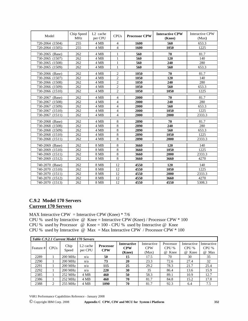
5308.345504550128 MB262740-2070 (1513)427036604550128 MB262740-2070 (1512)

2333.320004550128 MB262740-2070 (1511)122510504550128 MB262740-2070 (1510)1401204550128 MB262740-2070 (Base)

42703660366088 MB262740-2069 (1512)2333.32000366088 MB262740-2069 (1511)12251050366088 MB262740-2069 (1510)140120366088 MB262740-2069 (Base)

2333.32000289084 MB262730-2068 (1511)12251050289084 MB262730-2068 (1510)653.3560289084 MB262730-2068 (1509)280240289084 MB262730-2068 (1508)81.770289084 MB262730-2068 (Base)

2333.32000200044 MB262730-2067 (1511)12251050200044 MB262730-2067 (1510)653.3560200044 MB262730-2067 (1509)280240200044 MB262730-2067 (1508)81.770200044 MB262730-2067 (Base)

12251050105024 MB262730-2066 (1510)653.3560105024 MB262730-2066 (1509)280240105024 MB262730-2066 (1508)140120105024 MB262730-2066 (1507)81.770105024 MB262730-2066 (Base)

653.356056014 MB262730-2065 (1509)28024056014 MB262730-2065 (1508)14012056014 MB262730-2065 (1507)81.77056014 MB262730-2065 (Base)

12251050160044 MB255720-2064 (1505)653.3560160044 MB255720-2064 (1504)

Interactive CPW (Max)

Interactive CPW (Knee) Processor CPWCPUsL2 cache

per CPUChip Speed

MHzModel

C.9.2 Model 170 Servers Current 170 Servers

MAX Interactive CPW = Interactive CPW (Knee) * 7/6CPU % used by Interactive @ Knee = Interactive CPW (Knee) / Processor CPW * 100CPU % used by Processor @ Knee = 100 - CPU % used by Interactive @ KneeCPU % used by Interactive @ Max = Max Interactive CPW / Processor CPW * 100

7.56.492.381.77010904 MB255 MHz2238817.815.284.881.7704604 MB252 MHz1238612.710.989.158.3504604 MB252 MHz1238515.913.686.43530220n/a200 MHz1229225.421.778.329.225115n/a200 MHz122913227.472.623.32073n/a200 MHz1229035307017.51550n/a200 MHz12289

InteractiveCPU % @ Max

InteractiveCPU %

@ Knee

ProcessorCPU %

@ Knee

InteractiveCPW(Max)

InteractiveCPW

(Knee)

ProcessorCPW

L2 cacheper CPU

ChipSpeedCPUsFeature #

Table C.9.2.1 Current Model 170 Servers



Note: the CPU not used by the interactive workloads at their Max CPW is used by the system CFINTnnjobs. For example, for the 2386 model the interactive workloads use 17.8% of the CPU at their maximumand the CFINTnn jobs use the remaining 82.2%. The processor workloads use 0% CPU when theinteractive workloads are using their maximum value.

AS/400e Dedicated Server for Domino

----201204 MBn/a22409----15604 MBn/a12408----1030n/an/a12407

InteractiveCPU % @ Max

InteractiveCPU %

@ Knee

ProcessorCPU % @ Max

ProcessorCPU% @ Knee

InteractiveCPW

ProcessorCPW

L2 cacheper CPU

ChipSpeedCPUsFeature #

Table C.9.2.2 Dedicated Server for Domino

Previous Model 170 Servers

On previous Model 170's the knee of the curve is about 1/3 the maximum interactive CPW value.

Note that a constrained (c) CPW rating means the maximum memory or DASD configuration is theconstraining factor, not the processor. An unconstrained (u) CPW rating means the processor is the firstconstrained resource.

7.221.522.367319u7.221.522.367125c

2183

4.412.913.340319u4.412.913.340125c

2176

4.7149.729210u4.7149.729125c

2164

7.421.27.723114u7.421.27.723114c

2160

7.722.25.31673u7.722.25.31673c

2159

Interactive CPU % @ Knee

Interactive CPU % @ Max

Interactive CPW(Knee)

InteractiveCPW (Max)

Client / ServerCPW

Constrain /UnconstrFeature #

Table C.9.2.3 Previous Model 170 Servers



C.10 AS/400e Model Sxx Servers

For AS/400e servers the knee of the curve is about 1/3 the maximum interactive CPW value.

0.92.721.36423401222611.23.621.3641794822560.82.64012045501222081.13.240120366082207

S40

1.23.621.3641794822602.16.421.364998.6422593.71121.364583.3222585.416.117.251.531912257

S30

2.57.519.056.9759421663.610.716.749.7464.3221655.71711.935.8210121639.127.210.331113.812161

S20

11.133.48.124.473.11211911.935.75.416.245.412118S10

CPU % @ the Knee

CPU % @ MaxInteract

1/3 MaxInteract CPW

Max Inter CPW

Max C/S CPWCPUsFeature #Model

Table C.10.1 AS/400e Servers

C.11 AS/400e Custom Servers

For custom servers the knee of the curve is about 6/7 maximum interactive CPW value.

33.138.61757.12050.0455012234124.528.6900.01050.0366082340

S40

27.732.5496.8579.617948232218.521.5331.2386.417948232118.521.5184.4215.1998.642320

S30

25.029.2189.8221.47594217812.514.694.9110.775942177

S20

CPU % CPU % @ 6/7 Max Max Max CPUsFeature #ModelTable C.11.1 AS/400e Custom Servers

C.12 AS/400 Advanced Servers

For AS/400 Advanced Servers the knee of the curve is about 1/3 the maximum interactive CPW value.

For releases prior to V4R1 the model 150 was constrained due to the memory capacity. With the largercapacity for V4R1, memory is no longer the limiting resource. In V4R1, the limit of 4 DASD devices isthe constraining resource. For workloads that do not perform as many disk operations or don't require asmuch memory, the unconstrained CPW value may be more representative of the performance capabilities.An unconstrained CPW rating means the processor is the first constrained resource.



2.67.710.932.2650.04n/a21573910.732.2598.04n/a2156

4.513.510.732.2319.02n/a21556.820.315.932.2188.21n/a2154

53S

8.923.812.032.2138.01n/a2122103010.732.2111.51n/a21219.327.88.122.581.61n/a21209.929.810.832.291.01n/a21129.929.87.221.663.01n/a2111

50S

12.537.43.914.5351n/a21101030.13.19.4271n/a210940S

20.661.96.920.6351u227020.661.96.720.220.21c22701751.14.613.8271u22691751.14.613.820.21c2269

150

CPU % @ theKnee

CPU % @ MaxInteract

1/3 MaxInteract CPW

Max Inter CPW

Max C/S CPWCPUsConstrain /

UnconstrFeature #Model

Table C.12.1 AS/400 Advanced Servers: V4R1 and V4R2

2.67.710.430.7509.94n/a21573910.230.7459.34n/a2156

4.513.510.230.7278.82n/a21556.820.313.330.7162.71n/a2154

53S

8.923.811.530.7130.71n/a2122103010.230.7104.21n/a21219.327.87.721.477.71n/a212050S

9.929.810.330.787.31n/a21129.929.86.920.659.81n/a2111

12.537.43.713.833.31n/a21101030.13.19.427.01n/a2109

40S

20.661.96.920.633.31u227017.051.14.613.827.01c227033.0100.03.610.910.91u226933.0100.03.610.910.91c2269

150

CPU %@ the Knee

CPU % @ MaxInteract

1/3 MaxInteract CPW

Max Inter CPW

Max C/S CPWCPUsConstrain /

UnconstrFeature #Model

Table C.12.2 AS/400 Advanced Servers: V3R7

C.13 AS/400e Custom Application Server Model SB1

AS/400e application servers are particularly suited for environments with minimal database needs,minimal disk storage needs, lots of low-cost memory, high-speed connectivity to a database server, andminimal upgrade importance.

The throughput rates for Financial (FI) dialogsteps (ds) per hour may be used to size systems for customerorders. Note: 1 SD ds = = 2.5 Fl ds. (SD = Sales & Distribution).



238,073.64 95,229.464.0B396,789.40158,715.763.1H122313

164,655.74 65,862.294.0B274,426.23109,770.493.1H82312

FI ds/hr @ 65% CPU Utilization

SD ds/hr @ 65% CPU Utilization

SAPReleaseCPUsModel

Table C.13.1 AS/400e Custom Application Server Model SB1

C.14 AS/400 Models 4xx, 5xx and 6xx Systems

650509.9996409642162598459.3996409642153319278.8996409622152

188.2162.7996409612151148131.1996409612150

530

111.5104.265210241214481.677.7652102412143510

43.943.965210241214230.730.76527681214121.421.465276812140

500

3533.3502241213327275022412132

20.620.6502241213113.813.85016012130

400

V4R1 CPWV3R7 CPWDisk (GB)Maximum

Memory (MB)MaximumCPUsFeature CodeModel

Table C.14.1 AS/400 RISC Systems

23402095.93276812224317942095.9327688224045502095.94096012218936602095.94096082188

650

998.613401638442239583.3134087042223831913401638412237

640

464.3944.8409622182210944.8204812181

113.8944.820481218085.6944.820481217950944.8185612175

620

73.1175.45121213645.4175.43841213532.5175.43841213422.7175.438412129

600

V4R3 CPWDisk (GB) MaximumMemory (MB) MaximumCPUsFeature CodeModelTable C.14.2 AS/400e Systems



C.15 AS/400 CISC Model Capacities

16.83.9356121179.63.9340121157.32.992412114

P03

7.32.1161n/a P02CPWDisk (GB) MaximumMemory (MB) MaximumCPUsFeatureModel

Table C.15.1 AS/400 CISC Model: 9401

9.68.2401F067.37.9401E067.34.1241F045.52.1241F025.54.0241E045.51.6201D064.52.0241E024.41.6161D043.81.2161D023.61.3161C063.11.3121C04

CPWDisk (GB) MaximumMemory (MB) MaximumCPUsModelTable C.15.2 AS/400 CISC Model: 9402 Systems

5.517.17.95611005.517.13.9561S01

Interactive CPWC/S CPWDisk (GB) MaximumMemory (MB) MaximumCPUsFeature CodeTable C.15.3 AS/400 CISC Model: 9402 Servers

13.720.6801F2511.819.7801E2511.620.6801F209.719.7721E209.620.6721F109.76.4641D257.619.7401E106.84.8401D206.13.8401C255.34.8321D105.33.8321C205.13.8281B203.91.9201C102.91.9161B10


11.665.647.251221409.632.327.53841135

Interactive CPWC/S CPWDisk (GB) MaximumMemory (MB) MaximumCPUsFeature CodeTable C.15.5 AS/400 CISC Model: 9404 Servers



177.425615364F97148.825612804F95127.725610243F90116.625611524E9597.12567682F8096.725610243E9069.42565122E8057.02565121F7056.62563842D8040.01463841F6039.21462561E7032.31462561D7028.11461921E6027.81141921F5023.91461921D6020.054.81921B7018.198.01281E5017.167.0801F4515.154.8961B6013.767.0801F3513.867.0801E4513.398.01281D5010.867.0801D459.767.0721E359.327.4481B507.467.0721D356.513.7401B455.213.7401B404.613.7401B353.813.7361B30


177.4259.6153642052120.3259.615362205167.5259.6153612050

320

56.5159.38322204433.8159.383212043310

21.1117.41601204216.8117.4801204111.6117.47212040

300

16.823.61281203211.623.656120317.323.62412030

200

CPWDisk (GB) MaximumMemory (MB) MaximumCPUsFeature CodeModelTable C.15.7 AS/400 Advanced Systems (CISC)

11.668.586.5832224129.632.386.53841241130S

5.517.17.8128120102SS5.517.17.8128120102SG5.517.17.8128120102FS5.517.123.61281201020S

InteractiveCPWC/S CPWDisk (GB) MaximumMemory (MB) MaximumCPUsFeature CodeModel

Table C.15.8 AS/400 Advanced Servers (CISC)

