system dynamics: systems structure and behavior · to numerically evaluate the model the initial...

System Dynamics:

Systems Structure and Behavior

Lecture 2- May 22, 2017

Dr. Afreen Siddiqi Research Scientist, MIT

•  Adap&ve(thecapabili,esanddecisionrulesofagentsincomplexsystemschangeover,me)

•  Counterintui&ve(causeandeffectaredistantin,meandspace)

•  Characterizedbytrade-offs(thelongruniso;endifferentfromtheshort-runresponse,dueto,medelays.Highleveragepolicieso;encauseworse-before-beAerbehaviorwhilelowleveragepolicieso;engeneratetransitoryimprovementbeforetheproblemgrowsworse.

•  Governedbyfeedback(ac,onsfeedbackonthemselves)

•  Nonlinear(effectisrarelypropor,onaltocause,andwhathappenslocallyo;endoesn’tapplyindistantregions)

•  History-dependent(takingoneroado;enprecludestakingothersanddeterminesyourdes,na,on,youcan’tunscrambleanegg)

•  Dynamiccomplexityarisesduetointerac,onsamongdifferentagentsover,me.Systemswithevenafewelementscanexhibitdynamiccomplexity.

Review: Characteristics of Complex Systems

2

Modes of Dynamic Behavior

3

Figure Source: Sterman, 2000 4

Basic Modes of Behavior


Common Modes of Behavior

•  Arises from positive (self-reinforcing) feedback.

•  In pure exponential growth the state of the system doubles in a fixed period of time. •  Same amount of time to grow

from 1 to 2, and from 1 billion to 2 billion!

•  Common example: compound

interest, population growth

Exponential Growth

6 Figure Source: Sterman, 2000

Exponential Growth: Example

7


Some positive feedbacks underlying Moore’s Law

Paper folding exercise

•  Negative loops seek balance, and equilibrium, and try to bring the system to a desired state (goal).

•  Negative loops counteract change or disturbances.

•  Negative loops have a process to compare desired state to current state and take corrective action.

•  Pure exponential decay is characterized by its half life – the time it takes for half the remaining gap to be eliminated.

Goal Seeking

- +

+

Corrective Action +

11

Electricity generation [TWh] by fuel type in France from 1945 to 2012

A. Doufene, A. Siddiqi, and O. de Weck, (2014) “Dynamics of Technological Change: The Case of Nuclear Energy and Electric Vehicles in France”

Goal Seeking: Power Generation Capacity

12

•  This is the third fundamental mode of behavior.

•  It is caused by goal-seeking behavior, but results from constant ‘over-shoots’ and ‘under-shoots’

•  The over-shoots and under-shoots result due to time delays- the corrective action continues to execute even when system reaches desired state giving rise to the oscillations.

Oscillation


Oscillation: Example


•  Connection between structure and behavior helps in generating hypotheses

•  If exponential growth is observed -> some reinforcing feedback loop is dominant over the time horizon of behavior

•  If oscillations are observed, think of time delays and goal-seeking behavior.

•  Past data shows historical behavior, the future maybe different. Dormant underlying structures may emerge in the future and change the ‘mode’

•  It is useful to think what future ‘modes’ can be, how to plan and manage them

•  Exponential growth gets limited by negative loops kicking in/becoming dominant later on

Interpreting Behavior

15

•  Causal loop diagrams (CLDs) help –  in capturing mental models, and –  showing interdependencies and –  feedback processes.

•  CLDs cannot –  capture accumulations (stocks) and flows –  help in determining detailed dynamics

Stocks, Flows and Feedback are central concepts in System Dynamics

Limits of Causal Loop Diagrams

•  Stocks are accumulations, aggregations, summations over time

•  Stocks characterize/describe the state of the system – and accumulate past events

•  Stocks change with inflows and outflows

•  Stocks provide memory and give inertia by accumulating past inflows; they are the sources of delays.

•  Stocks, by accumulating flows, decouple the inflows and outflows of a system and cause variations such as oscillations over time.

Stock

Valve (flow regulator)

Flow

Source or Sink

Stocks

18

Birth rate [people/yr]

Death rate [people/yr]

Population [people]

Deposits [Rs/month]

Withdrawals [Rs/month]

Account Balance[Rs]

Change in expected orders rate [items/wk/wk]

Expected Orders [items/wk]

The manager’s belief of the order rate is a stock. It is a state of the system – a mental state.

Some Examples

•  Stock and flow diagramming were based on a hydraulic metaphor

•  Stocks integrate their flows:

•  The net flow is rate of change of stock:

Mathematics of Stocks

S t( ) = S t0( )+ I τ( )−O τ( )t0

t

∫ dτoutflow

inflow Stock S(t)

O(t)

I(t)

dSdt

= Net change in Stock = I(t)−O(t)

Stock t( ) = Stock t0( )+ Inflow τ( )−Outflow τ( )⎡⎣ ⎤⎦t0

t

∫ dτ

d Stock( )dt

= Inflow t( )−Outflow t( )

Snapshot Test: Freeze the system in time – things that are measurable in the snapshot are stocks.

Examples of Stocks and Flows

•  Inventory

•  Cash flow

•  Reactants

•  Reaction Rate

Accumulation and Memory

21

Time 0 10 20

Uni

ts/t

ime

10 5

15

Flow

30 0 10 20

units

100 50

150

Stock

30 Time

?

22

Carbon Emission rate [Tons/yr]

Carbon sequestration rate [tons/yr]

Atmospheric Carbon[Tons]

Discussion Point

What will happen (to stock of carbon in atmosphere) if we reduce carbon emissions?

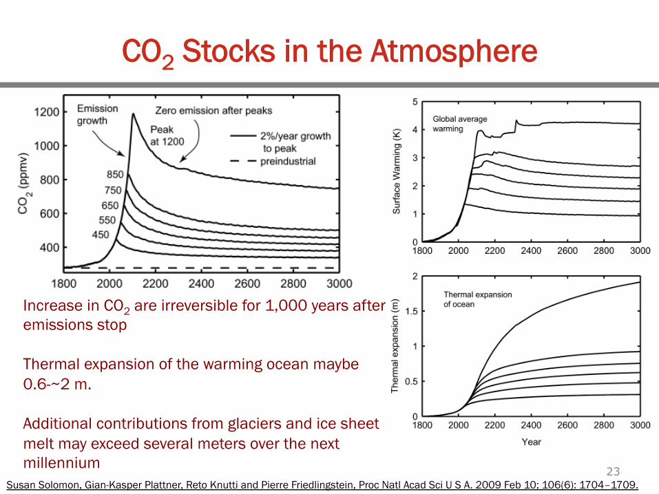
CO2 Stocks in the Atmosphere

23 Susan Solomon, Gian-Kasper Plattner, Reto Knutti and Pierre Friedlingstein, Proc Natl Acad Sci U S A. 2009 Feb 10; 106(6): 1704–1709.

Increase in CO2 are irreversible for 1,000 years after emissions stop Thermal expansion of the warming ocean maybe 0.6-~2 m. Additional contributions from glaciers and ice sheet melt may exceed several meters over the next millennium

•  Rates can be influenced by stocks, other constants (variables that change very slowly) and exogenous variables (variables outside the scope of the model).

•  Stocks only change via inflows and outflows.

•  Model systems as networks of stocks and flows linked by information feedbacks from the stocks to the rates.

24

Flow Rates

•  Is ‘interest rate’ (on a bond or savings certificate) a stock or a flow?

•  Employment rate?

•  What does the word “rate” mean in these cases?

25

Concept Check:

•  The underlying structure of the system defines the time-based behavior.

•  Consider the simplest case: the state of the system is affected by its rate of change.

From Structure to Behavior

•  First-order linear negative

feedback systems generate exponential decay

•  The net outflow is proportional to the size of the stock

•  The solution is given by: •  S(t) = So e-dt

d: fractional decay rate [1/time] Reciprocal of d is average lifetime units in stock.

Negative Feedback and Exponential Decay

Example: City Water Demand Simulation

28

•  The following mathematical equations specify the relationships between the variables (and constitute the definition of the model):

• 

•  It is assumed that migration (both in and out of the city) is proportional to the population, and values of ‘in migration’ and ‘out migration’ represent fractional values. To numerically evaluate the model the initial conditions and constants need to be defined. In this example, the following can be defined:

•  Population (t0) = 100,000 [people] •  Fractional birth rate = 0.04 [person/person/year] •  Fractional death rate = 0.02 [person/person/year] •  In migration = 0.005 [person/person/year] •  Out migration = 0.003 [person/person/year] •  Per capita coefficient = 75 m3/ person/ year

29

Population t( ) = Population t0( )+ Populationt0

t

∫ Increase Rate τ( )−Population Decrease Rate τ( )dτ

Population Increase Rate t( ) = in migration + fractional birth rate( )× Population t( )Population Decrease Rate t( ) = out migration + fractional death rate( )× Population t( )Urban Water Demand t( )= per capita coefficient× Population t( )

•  System dynamics has been the methodology of choice for multi-disciplinary and multi-actor problems.

•  The purpose is usually to address planning for intra- and inter-sectoral long-

term problems

•  System dynamics applications aim to integrate various physical, social and economic factors influencing water resources management

Applications in Water Resources Management

Ref: Winz et al 2009

32

Systemdynam

icssim

ulationin

water

resourcesm

anagement

1311

persisted,but

overthe

last10

yearsparticipatory

methods

havetaken

astrong

hold.R

equestsfor

participativeadaptive

managem

entw

ereincreasingly

voicedand

legislation,suchas

theE

uropeanW

aterD

irective,nowprioritises

stakeholderparticipation

inw

aterm

anagement(E

uropeanU

nion2007).

Fig.3

Atim

elineof

relevanttheoretical

andpractical

researchoutput.

Dow

nward

arrows

andunderlined

referencesindicate

where

participatorym

odellingw

asapplied

Ref: Winz et al 2009

Middle Rio Grande Basin Planning

33

CLD depicting key elements of water supply and demand

V. Tidwell, H. Passell, S. Conrad, and R. Thomas, “Systems Dynamics Modeling for community-based water planning: Application to the Middle Rio Grande”, Aquat. Sci. 66 (2004) 357–372.

Middle Rio Grande Basin Planning

34

Water supply and demand planning in the Middle Rio Grande Region


Key Stakeholders: Middle Rio Grande Water Assembly (MRGWA) Mid Region Council of Governments (MRCOG) City Utilities and Water Cooperatives Cooperative Modeling Team (CMT) General Public

System dynamics provided a mathematical framework for integrating the physical and social processes important to watershed management It provided an interactive interface for engaging the public. System dynamics modeling was used to assist in community-based water planning for a three-county region in north-central New Mexico, USA

35

Preferred Scenario Selected for 50-Year Water Plan


37 G. Di Baldassarre et al, (2015) “Debates – Perspectives on socio-hydrology: Capturing Feedbacks between physical and social processes”, Water Resources Research, pp4770-4781

Socio-Hydrology: Human Flood Interactions

•  Impacts of floods have risen dramatically in many regions of the world and the trend looks set to worsen in the future

•  There are many methods for quantitative assessment of risk

•  However, there is lack of fundamental understanding between interplay of physical and social processes.

•  Current frameworks do not capture or explain the emerging dynamics:

•  In some cases, “adaptation” plays out: occurrence of more frequent flooding is often associated with increasing resilience.

•  Empirical evidence shows that impacts of a flood event are lower when that event occurs shortly after a similar flood (society learns to cope and adapt)

•  Second type is “levee effect”: non-occurrence of frequent flooding (due to levees) is associated with increasing vulnerability to flooding. Paradoxically this increases the flood risk.


Socio-Hydrology: Human Flood Interactions

•  Flood risk is estimated as a combination of probability of flooding and the potential damages to society

•  In reality, there are “adaptation” and “levee effects”

•  There are coupled dynamics of floods and societies

•  Long term behavior emerges from the mutual interactions and feedbacks between social and physical systems


Green society

Technological society

F: relative flood damage D: population density H: flood protection level M: societal memory of floods

40 G. Di Baldassarre et al, (2015)

•  In adaptation case, the losses are between 25% to 40%

•  In levee effect, there is no flooding for a long period of time, the memory subsides, and society builds structures and increases its exposure. A large flood comes in 2048, causing catastrophic damage at 70%

•  Empirical historical research shows that population recovery is slow after 60% losses, and in some instances can lead to collapse.

Model Validation

•  The key factor influencing the acceptance and success of models is their practical usefulness.

•  A model is useful when it serves the purpose for which it was developed: it addresses the right problem at the right scale and scope.

•  Models are an abstraction of reality, and the greater the level of uncertainty and complexity of the problem, the more superficial objective comparisons between predicted results and observed data become.

•  Model validation is a social process where model structure and outcome are negotiated until judged valid and useful by all involved parties

•  Model usefulness requires transparency of the model development process and the model itself.

41

•  SDM will not provide exact solutions and answers. It is not suited to address well-defined operational problems

•  Differences in value judgements can dramatically influence which policies are ultimately recommended

•  Definition of the problem boundary, i.e. the model breadth, can be problematic. Modellers should only include variables if they contribute to generating the problem behaviour as experienced in reality

•  System dynamics modelling is more of an art than a science

Limitations of Systems Dynamics Modeling

Some Rules to Model By:

•  Develop a model for solving a problem –  Model should have clear purpose, do not include extraneous factors –  Start simple, add details as necessary over time

•  Approach model with skepticism –  Model is not reality (only a limited abstraction)

•  Use other tools and data –  Effective models use data and empirical analysis

•  Model should be developed iteratively and jointly with stakeholders –  Avoid black boxes, build understanding and trust

•  Validate with continuous testing, iteration, and stakeholder input 43

References

•  Business Dynamics: Systems Thinking and Modeling for Complex World, Sterman, McGraw Hill (2000).

•  I. Winz, G. Brierley and S. Trowsdale, “The Use of System Dynamics Simulation in Water Resources Management”, Water Resources Management (2009) 23:1301–1323

•  V. Tidwell, H. Passell, S. Conrad, and R. Thomas, “System dynamics modeling for community-based water planning: Application to the Middle Rio Grande”, Aquatic Sciences, (2004), 66: 357–372

•  G. Di Baldassarre et al, (2015) “Debates – Perspectives on socio-hydrology: Capturing Feedbacks between physical and social processes”, Water Resources Research, pp4770-4781

44

system dynamics: systems structure and behavior · to numerically evaluate the model the initial...

Documents