syst. biol. 57(1):86–103, 2008 issn: 1063-5157 print ...€¦ · syst. biol. 57(1):86–103, ......

Syst. Biol. 57(1):86–103, 2008Copyright c! Society of Systematic BiologistsISSN: 1063-5157 print / 1076-836X onlineDOI: 10.1080/10635150801886156

Efficiency of Markov Chain Monte Carlo Tree Proposals in Bayesian Phylogenetics

CLEMENS LAKNER,1,2 PAUL VAN DER MARK,2 JOHN P. HUELSENBECK,3 BRET LARGET,4 AND FREDRIK RONQUIST1,2

1Department of Biological Science, Section Ecology and Evolution, and2School of Computational Science, Florida State University, Tallahassee, Florida 32306-4120, USA;

E-mail: [email protected] (C. L.)3Department of Integrative Biology, 3060 VLSB 3140, University of California, Berkeley, Berkeley, CA 94720-3140, USA

4Departments of Botany and of Statistics, University of Wisconsin at Madison, Wisconsin 53706, USA

Abstract.— The main limiting factor in Bayesian MCMC analysis of phylogeny is typically the efficiency with which topologyproposals sample tree space. Here we evaluate the performance of seven different proposal mechanisms, including mostof those used in current Bayesian phylogenetics software. We sampled 12 empirical nucleotide data sets—ranging in sizefrom 27 to 71 taxa and from 378 to 2,520 sites—under difficult conditions: short runs, no Metropolis-coupling, and anoversimplified substitution model producing difficult tree spaces (Jukes Cantor with equal site rates). Convergence wasassessed by comparison to reference samples obtained from multiple Metropolis-coupled runs. We find that proposalsproducing topology changes as a side effect of branch length changes (LOCAL and Continuous Change) consistentlyperform worse than those involving stochastic branch rearrangements (nearest neighbor interchange, subtree pruning andregrafting, tree bisection and reconnection, or subtree swapping). Among the latter, moves that use an extension mechanismto mix local with more distant rearrangements show better overall performance than those involving only local or onlyrandom rearrangements. Moves with only local rearrangements tend to mix well but have long burn-in periods, whereasmoves with random rearrangements often show the reverse pattern. Combinations of moves tend to perform better thansingle moves. The time to convergence can be shortened considerably by starting with a good tree, but this comes at the costof compromising convergence diagnostics based on overdispersed starting points. Our results have important implicationsfor developers of Bayesian MCMC implementations and for the large group of users of Bayesian phylogenetics software.[Bayesian inference, Hastings ratio, Markov chain Monte Carlo, topology proposals.]

Bayesian inference was introduced to phylogeneticsin the last years of the 20th century (Li, 1996; Mau, 1996;Rannala and Yang, 1996; Mau and Newton, 1997; Yangand Rannala, 1997; Larget and Simon, 1999; Newtonet al., 1999; Huelsenbeck et al., 2000; Li et al., 2000) andhas become widely adopted since then (for reviews seeHuelsenbeck et al., 2001, 2002; Lewis 2001; Holder andLewis 2003. For a general discussion of Bayesian dataanalysis, see, for instance, Gelman et al., 2003). Typically,Markov chain Monte Carlo (MCMC) approaches basedon the Metropolis-Hastings algorithm (Metropolis et al.,1953; Hastings, 1970) are used to approximate the pos-terior distribution. A number of different MCMC pro-posal strategies have been applied but the efficiency ofthe different mechanisms has never been tested rigor-ously. Felsenstein (2004) appositely stated: “At the mo-ment the choice of a good proposal distribution involvesthe burning of incense, casting of chicken bones, magicalincantations and invoking the opinions of more presti-gious colleagues.” In this article, we suggest a frameworkfor testing the efficiency of tree proposals and apply it toseven mechanisms, including commonly used ones aswell as some that have not been considered in the litera-ture before.

In Bayesian phylogenetics, all inference is based onthe joint posterior distribution of evolutionary trees andsubstitution model parameters. Let ! = {", v} denote aphylogenetic tree with topology " and an associated setof branch lengths v and let # denote the set of all possi-ble phylogenies on N taxa. Furthermore, let $ = {#, %}denote the parameter space containing all phylogenetictrees and all possible attributions of values to the substi-tution model parameters (%). We focus here on the Jukes-Cantor model (Jukes and Cantor, 1969) without rate vari-ation among sites (JC), for which only the joint posterior

probability distribution of " and v needs to be approxi-mated since % is empty. The joint posterior distributionfor JC can formally be written as

f (", v|X) = f (X|", v) f (", v)!

"

"

vf (X|", v) f (", v) dv

where X denotes observed data.Calculating this distribution analytically would in-

volve summation over all possible trees and for eachtree integrating over all possible combinations of branchlengths (and usually also model parameters). This can-not be accomplished except for very small trees. In-stead, the posterior is typically estimated using a Markovchain, which generates dependent samples from thedistribution.

In practice, efficient proposal mechanisms are vital forthe chain to produce an adequate sample of the poste-rior probability distribution within the time constraintsfaced by most users. This is particularly true for complexmultimodal distributions, such as the distributions ontree space that result from most phylogenetic problems.In the latter, we can expect multiple posterior probabilitypeaks for each topology, corresponding to different com-binations of branch lengths, and—even worse—there isno obvious way of jumping between branch length peaksof different topologies. Several isolated areas of topologyspace with high probability mass, known as tree islands,may also have to be visited before an adequate sampleof the posterior is obtained. In phylogenetics, Markovchains that mix well move quickly among all the goodtrees, whereas chains that mix poorly tend to get stuck intree space. Markov chains that mix well may also be ex-pected to have shorter burn-in periods. However, bold

86

by guest on April 12, 2011sysbio.oxfordjournals.org

Dow

nloaded from

http://sysbio.oxfordjournals.org/

2008 LAKNER ET AL.—EFFICIENCY OF MCMC TREE PROPOSALS 87

proposals that tend to be rejected in later stages of anMCMC run may be advantageous during the burn-inphase because they may help the chain quickly explorelarge portions of the parameter space. More modest pro-posals generally have higher acceptance rates but areslower in providing adequate coverage and in movingbetween modes, resulting in longer burn-in periods andpoor mixing. Generally, proposals with intermediate ac-ceptance rates are considered optimal.

We focus here mostly on proposals that changetopology and branch lengths simultaneously. With JC,such proposals are sufficient for a working Markovchain, allowing us to test their performance individ-ually. The proposals we examine can be divided intotwo different classes: the branch-change proposals andthe branch-rearrangement proposals. The branch-changeproposals modify branch lengths or branch attachmentpoints continuously in a way that produces topol-ogy changes in some cases. Of this type, we con-sider the Continuous Change proposal (CC; Jow et al.,2002) and the LOCAL proposal (Larget and Simon,1999), used in the software packages PHASE (http://www.bioinf.manchester.ac.uk/resources/phase/) andBAMBE (Simon and Larget, 1998), respectively. The pro-grams MrBayes (Huelsenbeck and Ronquist, 2001; Ron-quist and Huelsenbeck, 2003) and PhyloBayes (Lartillotet al., 2007) also implement the LOCAL move.

The branch-rearrangement proposals—used in BEAST(Drummond and Rambaut, 2003), BADGER (Simon andLarget, 2004), MrBayes, PHASE, PhyloBayes, and alsoin Li et al. (2000) and Suchard et al. (2001)—can be di-vided into two subtypes: the pruning-regrafting movesand the swapping moves. In a pruning-regrafting move,a subtree is pruned from the rest of the tree and regraftedsomewhere else. We test two different strategies for se-lecting the regrafting point: (1) the point is chosen ran-domly; and (2) the attachment point is moved one branchat a time according to an extension probability, which re-sults in local rearrangements being favored. The moveswe consider are Random Subtree Pruning and Regraft-ing (rSPR), Extending Subtree Pruning and Regrafting(eSPR), and Extending Tree Bisection and Reconnection(eTBR).

In the second type of branch-rearrangement moves,which we refer to as the swapping moves, two subtrees

TABLE 1. Data sets used for the experiments.

No. of No. of TreeBASEData set taxa sites Type of data matrix accession no.

1 27 1949 rRNA, 18s M3362 29 2520 rDNA, 18s M5013 36 1812 mtDNA, COII (1–678), cytb (679–1812) M15104 41 1137 rDNA, 18s M13665 43 1660 rDNA, 18s M9326 50 378 Nuclear protein coding, wingless M34757 50 1133 rDNA, 18s M10448 59 1824 mtDNA, COII and cytb M18099 64 1008 rDNA, 28S M755

10 67 955 Plastid ribosomal protein, s16 (rps16) M174811 67 1098 rDNA, 18s M52012 71 1082 rDNA, internal transcribed spacer (ITS) M767

simply trade places. The moves we consider are Stochas-tic Nearest Neighbor Interchange (stNNI) and ExtendingSubtree Swapping (eSTS). We excluded random subtreeswapping from our comparison because preliminarydata indicated it was too bold to compete successfullywith the other moves. There is no meaningful way inwhich an extension mechanism can be applied to stNNIbecause its topology changes are always local. The stNNImove links the two subtypes of branch-rearrangementsbecause it can be understood both as a subtree swap andas a special case of subtree pruning and regrafting. All thetested proposals are available in the most recent sourcecode release of MrBayes (Ronquist and Huelsenbeck,2003, http://sourceforge.net/projects/mrbayes).

We assess the efficiency of the proposals using12 empirical DNA data sets selected from TreeBASE(http://www.treebase.org) and ranging in size from 27to 71 taxa and from 378 to 2520 sites (Table 1). The treeproposals are used to repeatedly sample the posteriorsof these data sets under difficult conditions, which al-lows us to challenge the proposals with relatively smalldata sets. In order to separately assess convergence andmixing behavior of the different proposals, we compareruns that are started from two sets of starting points:overdispersed trees and from trees that were sampledfrom the target distribution. We also try to eliminateother factors so that we can focus on the performanceof the tree proposals. Specifically, we use a fixed, rathersmall number of generations and we do not employMetropolis-coupling, a general technique for improv-ing mixing behavior in Bayesian MCMC phylogenetics(Geyer, 1991; Huelsenbeck et al. 2001). Finally, we usethe JC model to eliminate substitution model parame-ters and to make the posterior more difficult to samplefrom (Nylander, 2004). Convergence is assessed by com-parison to reference samples obtained using at least sixindependent Metropolis-coupled MCMC runs (Table 2).

METHODS

All analyses were conducted with a developer’s ver-sion of MrBayes 3.1.2, available from C.L. upon request.The parallel version of the program (Altekar et al., 2004)was used for the reference runs (see below). MCMC runswere deployed on a cluster of 57 dual AMD Athlon MP


Dow

nloaded from


88 SYSTEMATIC BIOLOGY VOL. 57

TABLE 2. Summary of the reference runs and number of generations for the test runs. The samples from the reference runs, which usedMetropolis-coupling and were run until the standard deviation of split frequencies was 0.005, were assumed to be accurate representations ofthe posterior probability distribution.

No. of trees in credible setNo. of generations No. of generations

Data set Proposal ratio until convergence 50% 90% 95% for the test runs

1 10 eTBR : 1 LOCAL : 1 stNNI 6,975,000 3 24 42 8 ! 106

2 1 LOCAL 1,131,000 2 4 5 1 ! 106

1 eTBR 323,0003 1 LOCAL 2,914,000 2 6 15 2 ! 106

1 eTBR 1,683,0004 5 eTBR : 1 LOCAL 6,183,000 4 78 189 7 ! 106

5 5 eTBR : 1 LOCAL 610,000 2 15 28 1 ! 106

6 5 eTBR : 1 LOCAL 4,305,000 7929 62,938 72,624 6 ! 106

7 8 eTBR : 1 LOCAL : 1 stNNI 6,771,000 7944 72,739 87,974 8 ! 106

8 5 eTBR : 1 LOCAL 3,940,000 26 417 778 5 ! 106

9 5 eTBR : 1 LOCAL 5,513,000 37 1273 3,105 6 ! 106

10 5 eTBR : 1 LOCAL 3,898,000 87,535 157,700 166,471 1 ! 106

11 5 eTBR : 1 LOCAL 8,547,000 17,081 122,217 141,448 9 ! 106

12 5 eTBR : 1 LOCAL 3,450,000 77,608 139,709 147,472 5 ! 106

2400+ processors running LINUX and a cluster of 64 dualG5 2.0 Ghz processors running Macintosh OS X at theSchool of Computational Science at Florida State Uni-versity. Jobs were distributed over the network clusterusing Condor version 6.7.1 (Litzkow et al., 1988).

The performance of the topology proposals was testedon 12 empirical DNA data sets (Table 1). Data set 6 wastaken from the literature (Brower, 2000) and submittedto TreeBASE as part of this study; the remaining data setswere obtained from previous submissions to TreeBASE.

All analyses were performed under the JukesCantor model with no rate variation across sites[MrBayes commands: lset nst=1 rates=equal; prsetstatefreqpr=fixed(equal)]. A uniform prior (all labeledtopologies equally likely) was used on topologies andan unconstrained, exponential prior with mean 0.1 wasused on branch lengths [prset topologypr=uniformbrlenspr=unconstrained:exponential(10)].

Convergence DiagnosticTo diagnose convergence among tree samples, we used

the average standard deviation of split frequencies (theestimated posterior probabilities of splits or taxon bipar-titions). Only splits that occurred in more than 10% ofthe samples in at least one of the runs were included inthe calculations because the frequency of the rare splitsis more difficult to estimate accurately and the rare splitsare less important in characterizing the tree sample.

Qualitatively similar results were obtained whenother cutoff levels and convergence-diagnostic statis-tics were used (maximum standard deviation andmaximum absolute difference of split frequencies; see on-line Supplementary Materials, available at http://www.systematicbiology.org).

Reference RunsTo obtain a reference sample of the posterior proba-

bility distribution for each data set, we ran six parallelruns, each using four Metropolis-coupled chains underthe default MrBayes heating schema (incremental heat-

ing with the temperature of chain i being 1/(1 + &i),with i " {0, 1, 2, . . . } and the tuning parameter & = 0.2).In every generation, a single swap was attempted be-tween a randomly drawn pair of chains. The runs werestarted from different random topologies and were sam-pled every 100 generations until the average standarddeviation of split frequencies fell below 0.005 for the last75% of the tree samples. In general, a mixture of topol-ogy proposals was used (Table 2). For data sets 2 and3, however, we used only the LOCAL update for threeruns and only the eTBR update for three runs. In bothcases, the LOCAL and eTBR runs converged to the samestationary distribution. The tuning parameter settingsfor all reference runs were as follows: eTBR extensionprobability 0.8, branch length multiplier 2 ln(1.6), LO-CAL & = 2 ln(1.1), and stNNI branch length multiplier2 ln(1.6).

Test RunsFor each data set, we generated 100 good starting trees

and 100 overdispersed random starting trees. The goodstarting trees were randomly drawn from the referencesample, whereas the overdispersed trees were generatedas follows: First, 10,000 random topologies were con-structed for each data set and for each pair of topologies,the Robinson-Foulds distance (Robinson and Foulds,1981) was calculated. Using a minimax and maximin dis-tance design algorithm (Johnson et al., 1990) a subset of100 topologies was determined to optimally fill the treespace. Finally, the branch lengths were all arbitrarily setto 0.1.

We tested three different tuning parameter settingsfor each proposal (Table 3). Setting I generated the mostmodest proposals, setting II intermediate proposals, andsetting III the boldest proposals. For the eTBR, eSPR, andeSTS proposals, we changed the extension probabilityrather than the branch length multiplier tuning param-eter, because the former has more effect on the behaviorof the proposal than the latter. For the rSPR move, wechanged the probability of proposing a topology change,which is likely to be of overriding importance when


Dow

nloaded from



TABLE 3. The tuning parameter settings tested for each tree proposal.

Tuning parameter settings for test runs

Proposal Tuning parameter Data seta I Data seta II Data seta III

rSPR Probability of topology change (Pr ) 0.8 0.9 0.95Multiplier (&) 2 ln(1.6) 2 ln(1.6) 2 ln(1.6)

eTBR Extension probability Pe 0.5 0.8 0.9& 2 ln(1.6) 2 ln(1.6) 2 ln(1.6)

eSPR Pe 0.5 0.8 0.9& 2 ln(1.6) 2 ln(1.6) 2 ln(1.6)

eSTS Pe 0.5 0.8 0.9& 2 ln(1.6) 2 ln(1.6) 2 ln(1.6)

stNNI & 2 ln(1.2) 2 ln(1.6) 2 ln(2.0)LOCAL & 2 ln(1.05) 2 ln(1.1) 2 ln(1.3)CC Standard deviation (' ) 1, 10 0.015 1, 10 0.02 1, 10 0.03

2, 3, 4 0.04 2, 4 0.06 2, 3, 4 0.085, 8, 9 0.03 3, 5, 8, 9 0.05 5, 8, 9 0.06

6 0.08 6 0.11 6 0.157 0.02 7, 11, 12 0.03 7, 11, 12 0.05

11, 12 0.021

aIf not applied to all data sets.

rSPR is used as the only proposal mechanism. For thestNNI and LOCAL moves, we varied the tuning param-eters that determine the boldness of the branch lengthmodifications. For the continuous change proposal, wefollowed the procedure used by Jow et al. (Vivek Gowri-Shankar, personal communication): the tuning param-eter (the standard deviation of the normal distributionused by the proposal) was adjusted beforehand for eachdata set to obtain an acceptance probability of approxi-mately 20%.

Each tuning parameter setting was run for a fixednumber of generations, using only a single chain (noMetropolis-coupling), on each of the 100 overdispersedand 100 good starting trees. The number of generationsfor these test runs was determined separately for eachdata set using the time to convergence for the refer-ence runs as a guide. Because the reference runs usedMetropolis-coupling and the test runs did not, we ex-pected a significant fraction of the test runs not to reachconvergence within the chosen number of generations.A test run was deemed to have converged if the averagestandard deviation of split frequencies, when the topol-ogy sample was compared to that of the reference run,was below 0.01 at the end of the run. The time to con-vergence was determined as the number of generationsthe chain was run before the the standard deviation ofsplit frequencies first fell below 0.01. The computationalcomplexity of the tested proposals is similar, so that thewall-clock time used per generation is essentially con-stant across the experiments.

In a separate experiment, we tested some of the pro-posals used above, which all change topology and branchlengths simultaneously, against comparable mixtures ofseparate topology and branch length proposals. The cho-sen proposals were rSPR (tuning parameter II, Table 3),eTBR (tuning parameter II), eSPR (tuning parameter II),and stNNI (tuning parameter I). To make the mixtures assimilar as possible to the corresponding joint proposals,we used the same algorithm for the mixtures and onlymodified it such that when a topology change was pro-

posed, branch lengths were left unmodified, with oldbranch lengths mapping into new ones as suggestedin the description of the proposals below. The mixtureswere only tested on the overdispersed starting trees. Forboth the mixtures and the joint proposals, we collectedinformation about the number of proposed and acceptedtopology changes.

Because most implementations use a combination ofseveral topology and branch length moves, we alsotested a mixture of all seven proposals and a mixtureof the five branch-rearrangement moves. In both cases,the proposals were chosen with equal probability at ev-ery step of the Markov chain. The tuning parameters forthese runs were adjusted to the best performing settingsfrom the individual runs.

Dependence of convergence success on the startingtree was assessed in several different ways. First, weused a (2 test of independence to examine whether sig-nificantly more runs converged for certain starting treesthan for others (P < 0.05). Second, to test whether runsstarted from random trees close to the good trees weremore likely to converge than others, the random treeswere ordered according to their likelihoods and accord-ing to their average Robinson-Foulds distances from asample of 1000 trees from the posterior (the post-burn-insample of the reference runs). The number of runs thathad reached convergence for each tree was summed overall proposals.

Finally, we graphically compared the variance in timeto convergence for runs started from the 100 overdis-persed trees with that for 100 runs started from the sametree (a randomly selected tree from the 100).

Topology ProposalsThe tested tree proposals can be roughly sorted from

bold to modest by first focusing on the expected NNIdistance between the candidate tree and the current tree(the minimum number of nearest neighbor interchangesrequired to go from one tree to the other). Among the


Dow

nloaded from



branch-rearrangement moves, the expected NNI dis-tance gives the rough sequence (from bold to modest)rSPR > eSTS > eTBR > eSPR > stNNI. For small trees,eSTS may actually be bolder than rSPR because the maxi-mum distance of the rSPR move is limited by the numberof branches in the tree, and subtree pruning and regraft-ing is, in itself, a more modest topology change thana subtree swap. Given the same extension probability,eTBR is typically more bold than eSPR since two attach-ment points are moved in eTBR and only one in eSPR.However, the distribution of topology changes is also dif-ferent. While the proposal distribution of eSPR has a longtail of rather distant rearrangements, the eTBR distribu-tion is more focused on less dramatic changes. Specif-ically, if d is the NNI distance and pe is the extensionprobability, the distribution is f (d) = (d + 1)pd

e (1 # pe )2

for TBR and f (d) = pde (1 # pe ) for SPR, in both cases as-

suming that the moves are not limited by the size ofthe tree. The stNNI move is the least bold because itonly involves one NNI rearrangement. The two branch-change moves (CC and LOCAL) may arguably be consid-ered more modest than all branch-rearrangement movesbecause they result in topological changes more rarelyand, when they do, the distance between the candidatetree and the current tree is always one NNI rearrange-ment. The CC move can be considered more modest inthat it makes less dramatic branch length changes thanLOCAL.

All seven tested tree proposals are briefly describedbelow. A more detailed description including the deriva-tion of the Hastings ratios can be found in the Appendix.The moves fall into two classes: (1) branch-change pro-posals (LOCAL and CC), which modify branch lengthsor branch attachment points in a way that sometimesleads to topology changes; and (2) branch-rearrangementproposals, which either prune and regraft subtrees(eSPR, eTBR, rSPR) or swap subtrees (stNNI, eSTS). Thebranch-rearrangement proposals either choose pruningand regrafting points or subtrees to swap using an ex-tension mechanism (eSPR, eTBR, eSTS), which favorslocal rearrangements, or at random (rSPR). The excep-tion is stNNI, which always involves minimal topologychanges.

LOCAL.—This update mechanism was introduced byLarget and Simon (1999) and first used in their soft-ware package Bayesian Analysis in Molecular Biologyand Evolution (BAMBE). It consists of two independentsteps that could form separate update mechanisms. Thefirst step changes a subtree attachment point, the secondchanges three branch lengths. For detailed descriptionsof the move see Larget and Simon (1999), Larget (2005),and Holder et al. (2005).

Continuous change (CC).—Introduced by Jow et al.(2002), CC is primarily a branch length proposal. It firstpicks a branch b at random, whose length is v. A valueu is drawn from N(0, ' ), where ' is a tuning parame-ter, and we propose the new branch length v$ = |v + u|.If v + u < 0 and b is internal, then, with equal probabil-ity, the topology is changed to one of the two alternativeNNI rearrangements centered on b and v$ becomes the

length of the new branch. In all other cases, the topologyremains unchanged. The proposal ratio of the CC moveis 1 (Appendix).

Stochastic nearest neighbor interchange (stNNI).—Thestochastic nearest neighbor interchange we implementedfirst picks a random interior branch bx with the lengthvx. This branch has four subtrees attached to its ends.Randomly label the two subtrees at one end A and Band the two subtrees at the other end C and D. Sub-tree A sits on a branch with the length va , etc., so thatthe five branches affected by this move can be collectedin the local branch length vector v = (va , vb , vc , vd , vx).Now, with probability 1/3 swap A and C ; with probabil-ity 1/3 swap B and C ; and with probability 1/3 leave thetopology unchanged. Finally, propose the new branchlengths v$ = {mava , mbvb , mcvc , mdvd , mxvx}, where eachmi represents an independent application of the multi-plier move described in the Appendix. The proposal ratiofor the topology part of this move is 1; for the factor ofthe multiplier part see the Appendix.

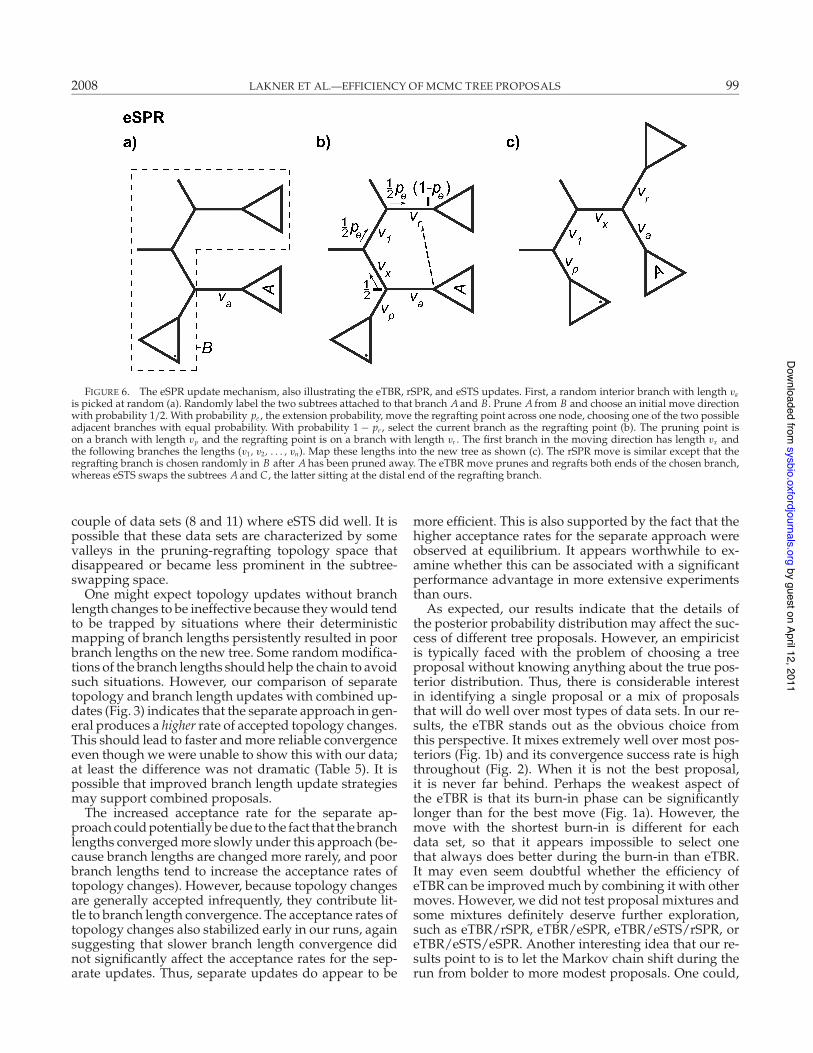
Extending subtree pruning and regrafting (eSPR).—TheeSPR proposal first picks a random interior branch baof length va (Figure 6a). Randomly label the subtrees at-tached to that branch A and B. Consider B as rooted atba and arbitrarily label each pair of descendant branchesin B as left and right descendants. Now prune A from Band choose a regrafting point for A on B using the fol-lowing mechanism (see Fig. 6b). With probability 1/2, tryto move the regrafting point left in B, and with probabil-ity 1/2 try to move it right. With probability pe , which isa tuning parameter called the extension probability, movethe regrafting point across one node to either the leftor right descendant branch with equal probability. Withprobability 1 # pe , choose the current branch as the re-grafting point. If the current branch is a terminal branch,the extension mechanism stops and the current branchis called a constrained regrafting point. If the extensionmechanism could have proceeded at least one step far-ther, the regrafting point is unconstrained.

Label the two branches at the pruning point bx and b p,where bx is the branch in the chosen movement directionand b p is the other branch (the pruning branch). Label thebranch chosen for regrafting br (the regrafting branch)and the branches traversed during the extension phase(b1, b2, . . . , bn; see Fig. 6). In the new topology, branchesb p, br , ba can be mapped together with their lengths(vp, vr , va ) into branches that define the same splits,whereas the branches in the vector (b1, b2, . . . bn) and theirlengths can be mapped into equivalent branches that dif-fer only in the placement of the leaves in A. This leavesus with bx and vx, which are mapped into the regraftingpoint in the direction of the reverse move (see Fig. 6c).

After completing these branch length transfers, we ap-ply the multiplier move independently to the branchlengths v = (va , vx) to give the new branch lengths v$ =(mava , mxvx). See the Appendix for the derivation of theHastings ratio.

In clock trees, the subtree A cannot be picked ran-domly; it will always have to be from the younger (non-root) end of the chosen interior branch. In standard


Dow

nloaded from



unrooted trees, however, it is probably suboptimal toenforce a consistent rooting such that SPR moves alwayschange one of the two attachment points of a given inte-rior branch. This is because the rooted version of the SPRproduces a topology space that is less well connectedand presumably more difficult to traverse than that ofthe unrooted version we used here.

Extending tree bisection and reconnection (eTBR).—This isthe same move as eSPR except that the extension mecha-nism is applied to both ends of the picked interior branchba . Also, when the pruning and regrafting points are thesame, we always modify the lengths va and vx, nevervp.

Extending subtree swapper (eSTS).—This move is simi-lar to the stNNI move in that it involves a swap of twosubtrees. However, the swapped subtrees need not benearest neighbors; they are chosen by an extension mech-anism and can be arbitrarily distant (Appendix).

Random subtree pruning and regrafting (rSPR).—Thismove is similar to eSPR except that the regrafting branchis picked randomly from the branches in subtree B. Be-cause an extension mechanism is not used, the proposalratio for the topological change is always 1 and the ra-tio for the branch length change is identical to the onefor eSPR. To increase the frequency of branch lengthchanges without topology modifications, which is im-portant when rSPR is used as the only tree proposal, weintroduced a tuning parameter pr , the rearrangement prob-ability. With probability pr , we selected a regrafting pointamong the branches in B other than the pruning point.With probability 1 # pr , we would force the regraftingpoint to be the same as the pruning point.

Visualizing Tree SpaceThe Mesquite (Maddison and Maddison, 2005) Tree

Set Visualization Module (TSV; Hillis et al., 2005,http://comet.lehman.cuny.edu/treeviz/) was used to il-lustrate tree space via multidimensional scaling on atopology sample using unweighted Robinson-Fouldsdistances. The topology sample consisted of 5000 sam-ples drawn from the posterior (i.e., from the referenceruns) and 500 samples from each of the chain paths thatwe wanted to plot in the space. The x- and y-coordinatesof each topology were extracted from the postscript filegenerated by TSV. These coordinates were used to plotthe posterior probability of each topology and the chainpaths in the resulting space.

RESULTS

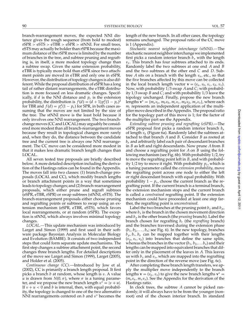
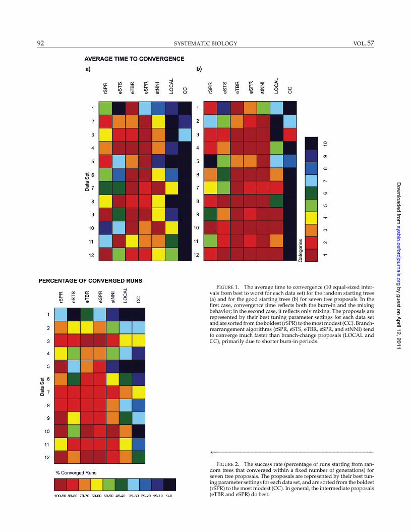
For each proposal, we tested three different sets of tun-ing parameters (Table 3), where the first set (I) gave moremodest proposals, the second set (II) intermediate pro-posals, and the third set (III) bolder proposals. The timeto convergence and the convergence success rate weremeasured under two different scenarios. First, we startedfrom 100 overdispersed random starting trees (Fig. 1a). Inthis situation (random starting trees), we expect the time toconvergence to reflect both the burn-in time and the mix-ing efficiency. Second, we started from 100 trees drawn

from the posterior distribution (i.e., the reference sam-ple; Fig. 1b). In this case (good starting trees), the time toconvergence should be determined solely by the mixingbehavior since the burn-in period is negligible.

Our most striking result is that the branch lengthmoves (CC and LOCAL) do very poorly compared tothe branch-rearrangement moves (Fig. 1). This is ap-parently due primarily to long burn-in times for CCand LOCAL, but mixing is also slow, in particular forCC (Fig. 1b). Among the branch-rearrangement moves,eTBR and eSPR do particularly well. Their superiorperformance is the result of both short burn-in timesand rapid mixing. The more modest stNNI move mixesslightly better for some data sets than both eTBR andeSPR (Fig. 1 b) but its burn-in time is considerably longer(Fig. 1a). The boldest proposals, rSPR and eSTS, occasion-ally do well but their performance is unpredictable. TherSPR move might be expected to perform poorly on largetrees, because the rejection rate presumably increaseswith tree size, but we could not detect such a trend in ourdata.

Focusing on the success rate (the percentage of runsthat converged within the predefined number of gener-ations) instead of the time to convergence, the picturechanges slightly (Fig. 2). We show these data only for theruns starting from overdispersed trees, because the suc-cess rate was uniformly high when starting from goodtrees. The boldest proposal, rSPR, does much better whenjudged by this criterion than by the time to convergence.On average, the rSPR move achieves convergence muchslower than eTBR and eSPR (Fig. 1), but it succeeds witha similar number of runs within a fixed number of gener-ations (Fig. 2). For some data sets (5 and 9), it actually suc-ceeds with more runs than eTBR and eSPR. Thus, rSPRcan be described as a safe but slow proposal mechanism.The same thing cannot be said for eSTS; its success rateis considerably lower than that of eTBR and eSPR eventhough it is a bolder proposal.

To illustrate the effect of changing the tuning param-eters, we also give the success rates for all three tuningparameter settings (Table 4). The tuning parameters tendto have a distinct but not dramatic effect, with the inter-mediate settings (II) often doing better than the two ex-treme settings. An obvious exception is LOCAL, wherethe success rate was very similar for all tuning parametersettings.

The overall acceptance rate was not a good indicatorof convergence success (see online Supplementary Ma-terials). Convergence success correlated better with thenumber of accepted topology changes and the averageNNI distance of the accepted proposals, but the correla-tion was far from perfect. For data set 12, for instance,rSPR(II) always converged, whereas eTBR(III) was do-ing considerably worse at 87%. Yet the overall accep-tance rate was similar, and the number and topologicaldistance of accepted topological changes were roughlythe same as well. A possible explanation is that a fewsuccessful distant topology changes helped shorten theburn-in or improve the mixing significantly for the rSPRmove on this data set.


Dow

nloaded from



FIGURE 1. The average time to convergence (10 equal-sized inter-vals from best to worst for each data set) for the random starting trees(a) and for the good starting trees (b) for seven tree proposals. In thefirst case, convergence time reflects both the burn-in and the mixingbehavior; in the second case, it reflects only mixing. The proposals arerepresented by their best tuning parameter settings for each data setand are sorted from the boldest (rSPR) to the most modest (CC). Branch-rearrangement algorithms (rSPR, eSTS, eTBR, eSPR, and stNNI) tendto converge much faster than branch-change proposals (LOCAL andCC), primarily due to shorter burn-in periods.

%###########################################

FIGURE 2. The success rate (percentage of runs starting from ran-dom trees that converged within a fixed number of generations) forseven tree proposals. The proposals are represented by their best tun-ing parameter settings for each data set, and are sorted from the boldest(rSPR) to the most modest (CC). In general, the intermediate proposals(eTBR and eSPR) do best.


Dow

nloaded from



TABLE 4. Convergence success (percentage of runs that reached convergence) for runs started from overdispersed random trees (bold: bestvalue for the data set; shaded cells: significantly worse than best value).

Percentage of converged runs

rSPR eTBR eSPR eSTS stNNI LOCAL CC

Data set I II III I II III I II III I II III I II III I II III I II III

1 32 30 27 32 46 43 14 30 16 6 4 4 12 10 9 8 8 7 4 6 22 73 66 69 60 60 55 47 70 63 59 67 51 57 49 37 38 29 32 29 34 373 78 71 83 85 89 93 86 83 92 72 81 84 81 74 72 65 57 57 55 47 604 59 65 62 72 67 59 63 68 70 51 55 51 52 47 28 30 20 21 16 7 85 81 90 85 57 75 72 46 89 87 25 39 35 16 11 16 5 3 3 3 6 66 68 67 73 86 80 69 70 80 83 43 40 40 66 61 43 42 42 37 13 6 57 80 70 78 88 79 69 85 80 80 80 82 75 80 83 78 69 73 62 57 64 418 74 81 73 81 87 86 82 87 88 71 82 85 70 65 35 39 29 30 29 22 189 96 97 95 76 89 80 70 83 89 49 58 61 70 61 51 43 45 41 37 26 17

10 82 79 100 95 84 51 78 87 61 52 50 31 95 97 90 68 76 75 0 0 011 60 49 43 78 80 55 84 85 84 86 82 86 81 82 76 65 62 58 20 8 112 100 100 100 95 95 87 88 95 97 73 73 70 83 85 83 74 73 75 46 37 15

Across all data sets, the stNNI(I) move stood out interms of its success in modifying the topology. For dataset 2, for instance, stNNI(I) had more than 11,000 ac-cepted topology changes; the closest competitors hadlittle more than 3000. Whereas the best LOCAL move,LOCAL(I), succeeded with only 0.4% of its attempts tochange the topology for this data set, stNNI(I) succeededmore than four times as often (1.7%). A high number ofaccepted topology changes correlated to some degreewith rapid mixing (Fig. 1b) but not at all with burn-in times (Fig. 1b). Short burn-in times were more oftenassociated with a large distance of accepted topologychanges. The obvious exception was eSTS, which oftenhad long burn-in times despite making radical topologymodifications.

For the proposals using the extension mechanism,increasing the extension probability resulted in boldertopology rearrangements and fewer accepted proposals.The number of accepted topology changes, however, wasless affected than the overall acceptance rate. In somecases, the number of accepted topology changes actuallyincreased when going from the lowest (0.5) to the inter-mediate (0.8) extension probability. The boldness of theaccepted topology changes also often peaked at an exten-sion probability of 0.8. It is possible that this contributedto the intermediate tuning parameter settings (II) of thesemoves (eSTS, eTBR, eSPR) converging so well (Table 4).

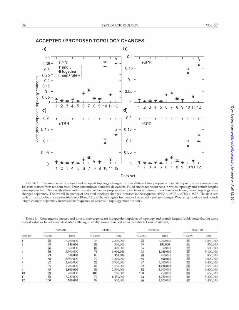
When comparing different moves, it is clear that boldermoves had lower acceptance probabilities than moremodest moves (filled circles, Fig. 3). For instance, stNNItopology changes were, on average, more than threetimes as likely as rSPR changes to be accepted. The ac-ceptance rates also correlated strongly with the topolog-ical variance of the posterior distribution. The highestacceptance rates were observed for data sets with largenumbers of trees in their 95% credibility sets, such asdata sets 6, 7, 10, and 12 (Table 2). The three data sets (2,3, and 5) with the smallest number of trees in their credi-ble sets also had the lowest acceptance rates for topologychanges. In other words, the more informative the dataare about the topology, the more difficult it is for topologyproposals to get accepted.

The branch-rearrangement proposals we studied allmodify branch lengths in the neighborhood of an at-tempted topology change by using the multiplier move(see Methods). An alternative possibility is to map oldbranch lengths into the new tree without changing theirvalues at all. We did not use such proposal mechanismsin the main experiment because their performance can-not be evaluated separately; they must be combined withbranch length proposals to produce a working Markovchain, and this would have complicated the compari-son with the branch-change moves, CC and LOCAL.However, we did evaluate mixtures of separate topol-ogy and branch length proposals against our combinedapproach in a separate experiment. In this experiment,the normal stNNI, eSPR, eTBR, and rSPR moves werecontrasted with moves that were programmed identi-cally except that the branch lengths were modified onlywhen the proposed topology was the same as the currentone.

In this experiment, we found that the probability ofaccepting a proposed topology change was higher whentopology and branch lengths were updated separately(open circles, Fig. 3) than when they were updated si-multaneously (filled circles). The difference was smallfor many data sets but rather pronounced for the oneswith many trees in their credible sets (data sets 10 and 12in particular). Despite the success of the separate propos-als in modifying topology, the convergence success andthe times to convergence were roughly comparable tothat of the corresponding combined proposals (Table 5).Thus, the higher rate of accepted topology changes forseparate proposals (Fig. 3) was not reflected in significantimprovements in the convergence behavior.

For most data sets, combinations of the moves per-formed better when branch-change proposals were ex-cluded (Table 6). With respect to time to convergence, thecombined approach often outperformed the single pro-posal approach, especially in the runs that were startedfrom overdispersed trees.

By visualizing tree space using multidimensional scal-ing and by following the chain paths through this space,it is possible to illustrate the mixing behavior of the


Dow

nloaded from



FIGURE 3. The number of proposed and accepted topology changes for four different tree proposals. Each data point is the average over100 runs started from random trees. Error bars indicate standard deviations. Filled circles represent runs in which topology and branch lengthswere updated simultaneously (the standard version of the tree proposals); empty circles represent runs where branch lengths and topology werechanged separately. The overall frequency of accepted topology changes increases in the sequence stNNI > eSPR > eTBR > rSPR. The data setswith diffuse topology posteriors (data sets 10 and 12) also have a higher frequency of accepted topology changes. Proposing topology and branchlength changes separately increases the frequency of successful topology modifications.

TABLE 5. Convergence success and time to convergence for independent updates of topology and branch lengths (bold: better than or sameas best value in Tables 7 and 4; shaded cells: significantly worse than best value in Table 4; Conv.: converged).

rSPR (II) eTBR (I) eSPR (II) stNNI (I)

Data set % Conv. Time % Conv. Time % Conv. Time % Conv. Time

1 25 7,700,000 45 7,300,000 24 7,700,000 15 7,850,0002 69 350,000 54 500,000 69 350,000 54 550,0003 76 550,000 82 400,000 86 350,000 79 500,0004 56 5,300,000 76 3,900,000 73 4,050,000 47 5,100,0005 93 350,000 85 350,000 78 450,000 22 850,0006 88 3,500,000 79 3,200,000 86 800,000 70 4,000,0007 82 3,900,000 75 3,900,000 87 3,000,000 77 3,400,0008 85 1,700,000 84 1,550,000 92 1,100,000 66 2,550,0009 95 1,800,000 84 2,500,000 82 2,500,000 64 3,600,00010 89 700,000 100 700,000 100 750,000 90 650,00011 63 7,250,000 79 6,450,000 92 4,750,000 90 5,300,00012 100 500,000 99 850,000 96 1,100,000 87 1,400,000


Dow

nloaded from



TABLE 6. Convergence success and time to convergence for combinations of proposals (bold: better than or same as best value in Tables 7and 4; shaded cells: significantly worse than best value in Table 4; Conv.: converged).

All moves Branch-rearrangement moves

Data set % Conv.a Time 1a Time 2b % Conv.a Time 1a Time 2b

1 24 7,750,000 2,308,555 36 7,550,000 1,943,4802 68 350,000 6,395 73 300,000 5,4253 79 500,000 14,585 85 400,000 13,2204 66 4,350,000 538,990 68 4,150,000 520,6805 84 400,000 31,765 81 400,000 29,7606 88 2,750,000 965,780 88 2,750,000 1,019,6507 87 2,600,000 969,225 84 3,050,000 997,1658 77 1,900,000 214,615 81 1,550,000 186,4909 86 2,200,000 235,690 94 2,100,000 354,690

10 100 550,000 402,310 100 550,000 384,12511 89 5,000,000 1,847,570 94 4,850,000 1,923,09512 100 600,000 306,475 100 650,000 306,000

aRuns started from overdispersed starting trees.bRuns started from trees with high posterior probability.

different proposals in more detail. For this purpose, wechose our smallest and most difficult data set (data set1), which has only three topologies in its 50% credibleset (1, 2, and 3), whereas some topologies in its 90%credible set (exemplified by topology 4) are separatedfrom these by a broad valley (Fig. 4). Clearly, the suc-cess of sampling the posterior depends on having theright proportion of trees sampled from the space aroundtopologies 1 to 3 and from the space around topology4, on opposite sides of the valley. The more times thechain can cross that valley, the more likely it should be toget the proportions right. On average, eTBR outperformsLOCAL on this data set and it also crosses the valleymore often, as evidenced by both short and long runs(Fig. 4). In the subsample of 500 trees used to generatethe plots, the eTBR crossed the valley multiple times be-tween adjacent sampling points (Fig. 4a and c), whereasthe LOCAL crossed the valley only once (Fig. 4b) or twice(Fig. 4d).

Because we used the same set of starting trees forall proposals, we could examine the effect of the start-ing point on the convergence behavior across proposals.Among the overdispersed trees, some should offer betterchances of rapid convergence than others because theyare closer to the good trees. Among the good trees, sometrees might be better starting points than others becausethey are situated in the middle of the posterior distri-bution rather than at some extreme. However, we couldfind no such effects (see Methods for details). Among the100 starting trees, whether overdispersed or drawn fromthe posterior, it was not true that particular trees weremore often associated with successful runs than othertrees. Similarly, closeness to the good trees in topologyspace did not predict convergence success, nor did start-ing trees with a high initial likelihood result more oftenin convergence than other trees.

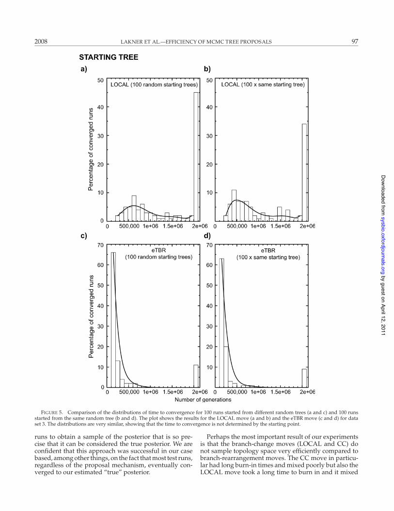
To illustrate the lack of starting-point dependence, wecompared 100 runs started from different overdispersedtrees with 100 runs started from the same tree (this treebeing one of the 100). For this experiment we used theLOCAL and eTBR moves. As expected, the distribution

of convergence times was essentially identical regardlessof whether the starting points were different or the same(Fig. 5). This was true both for the LOCAL move and foreTBR, even though the mixing behaviors of these twomoves are quite different, and hence also their distribu-tions of convergence times.

The starting-point independence among random treesand among good trees contrasts starkly with the differ-ence between them. When the runs were started fromgood trees, convergence was reached much faster thanif the runs were started from random trees. The differ-ence in convergence time was an order of magnitude formany data sets (Tables 7 and 8).

Finally, some general patterns are worth pointing out.Despite expectations to the contrary, we could not detectany correlation between the difficulty of sampling theposterior and the number of taxa, the number of charac-ters, or the number of trees in the 50% credible set (Tables1 and 2, Fig. 1). Overall, the most difficult data set wasdata set 1, which had the smallest number of taxa andamong the smallest number of trees in its credible set.The two data sets with the smallest number of characters(6 and 10) were more difficult than average and the twodata sets with the largest number of characters (1 and2) were among the most difficult (Fig. 1a). Apparently,the exact shape of the posterior distribution was moreimportant in determining the sampling difficulty of ourdata sets than factors such as tree size, number of char-acters, or number of trees in the credible set. It shouldbe pointed out, however, that the variation in tree sizeand number of characters of the tested data sets is rathersmall.

DISCUSSION

To evaluate the efficiency of different tree proposalsin sampling the true posterior probability distribution,it is necessary to know the latter. Typically, it is difficultto calculate this distribution, even for simulated data,unless the tree is very small. Our approach relies on us-ing Metropolis-coupling and several independent, long


Dow

nloaded from



FIGURE 4. The mixing behavior of the eTBR (a and c) and LOCAL (b and d) proposals on data set 1. For each proposal, one run that convergedwithin approximately 350,000 generations is shown (a and b), as well as one run that had not converged within 10 million generations (c andd). All four runs were started from trees sampled from the posterior probability distribution. For data set 1, the three most probable topologies(1, 2, and 3) are similar to each other but some other topologies (exemplified by 4) in the 90% credible set are separated from these by a distinctvalley in topology space (a and b). Following the chain path through an evenly spaced subsample of 500 points from each run shows that theeTBR move crosses the valley much more frequently (a and c) than the LOCAL move (b and d). Gray dots indicate trees from the reference run.


Dow

nloaded from



FIGURE 5. Comparison of the distributions of time to convergence for 100 runs started from different random trees (a and c) and 100 runsstarted from the same random tree (b and d). The plot shows the results for the LOCAL move (a and b) and the eTBR move (c and d) for dataset 3. The distributions are very similar, showing that the time to convergence is not determined by the starting point.

runs to obtain a sample of the posterior that is so pre-cise that it can be considered the true posterior. We areconfident that this approach was successful in our casebased, among other things, on the fact that most test runs,regardless of the proposal mechanism, eventually con-verged to our estimated “true” posterior.

Perhaps the most important result of our experimentsis that the branch-change moves (LOCAL and CC) donot sample topology space very efficiently compared tobranch-rearrangement moves. The CC move in particu-lar had long burn-in times and mixed poorly but also theLOCAL move took a long time to burn in and it mixed


Dow

nloaded from



TABLE 7. Average time to convergence for runs started from overdispersed random trees (bold: best value for the data set; only values forthe best tuning parameter settings are shown).

Average number of generations until convergence

Data set rSPR eTBR eSPR eSTS stNNI LOCAL CC

1 7,600,000 7,250,000 7,750,000 8,000,000 7,850,000 7,900,000 8,000,0002 400,000 450,000 350,000 450,000 550,000 750,000 700,0003 550,000 350,000 200,000 450,000 450,000 1,300,000 950,0004 4,900,000 4,200,000 4,350,000 4,850,000 4,800,000 6,400,000 6,700,0005 450,000 500,000 350,000 800,000 900,000 1,000,000 1,000,0006 4,250,000 3,150,000 3,050,000 5,300,000 4,050,000 5,050,000 5,900,0007 4,300,000 2,650,000 3,200,000 4,450,000 2,800,000 3,800,000 5,850,0008 2,450,000 1,650,000 1,550,000 1,300,000 2,400,000 4,450,000 4,550,0009 2,100,000 2,150,000 2,250,000 3,700,000 3,200,000 4,550,000 5,050,000

10 750,000 600,000 700,000 900,000 550,000 800,000 1,050,00011 7,350,000 5,800,000 5,450,000 5,450,000 5,400,000 6,900,000 8,800,00012 650,000 1,300,000 1,150,000 2,400,000 1,750,000 2,250,000 4,000,000

well only for the largest trees. We do not think that theseresults are due to suboptimal tuning parameter settingsin our experiments. The LOCAL tuning parameter haslittle influence on performance and the CC tuning pa-rameter was optimized for each data set according to thesuggestions by Jow et al. (2002). One could argue thatthe LOCAL move, for instance, is inefficient solely be-cause it proposes topology changes less often than themost similar branch-rearrangement move, stNNI. How-ever, even if we restrict our attention to the proposedtopology changes, stNNI still succeeded better than LO-CAL at getting these accepted. This was true for all ourdata sets, the difference usually being significant. In con-clusion, we recommend that CC and LOCAL be usedonly in combination with branch-rearrangement moves.In general, stNNI should perhaps also be combined withother branch-rearrangement proposals.

The rSPR move is commonly used in phylogenet-ics MCMC software, but we found its performance tobe unpredictable. In some cases where the move wassuccessful (data sets 2, 5, and 9), the reason appears to bethat it found a very small set of good trees in a large treespace more effectively than other moves. It is character-istic for these data sets that the good overall performanceof rSPR is due entirely to short burn-in times because itsmixing is poor (Fig. 1a and b).

TABLE 8. Average time to convergence for runs started from trees with high posterior probability (good trees; bold: best value for the dataset; only values for the best tuning parameter settings are shown).

Average number of generations until convergence

Data set rSPR eTBR eSPR eSTS stNNI LOCAL CC

1 1,841,250 1,224,560 2,833,390 6,602,330 3,829,935 5,370,930 7,264,8902 16,270 8,155 6,940 12,675 3,905 24,400 17,1753 24,840 17,450 11,605 22,660 5,080 149,390 28,7104 957,695 660,725 618,935 1,132,205 827,015 1,548,300 2,917,4155 97,020 37,820 35,540 57,020 18,350 69,435 78,7406 2,290,465 1,144,960 1,109,165 3,430,320 1,211,845 2,178,805 5,392,4907 1,433,180 759,750 1,107,670 1,655,070 1,071,670 1,184,080 2,943,6808 630,205 313,860 296,760 147,710 207,485 1,805,050 2,929,4009 740,560 287,395 362,585 462,105 250,405 336,775 1,181,92510 599,050 489,500 592,880 876,940 393,220 686,470 4,151,13511 4,127,870 1,951,790 2,359,795 2,535,100 1,744,760 3,262,490 7,507,36012 493,225 403,780 429,145 378,080 235,065 393,755 2,598,430

In general, one might expect rSPR to do worse as thetrees get larger, because the proportion of local topol-ogy changes decreases rapidly with increasing tree sizefor this move. This could possibly contribute to thepoor performance of rSPR on data sets 10 and 11. It ismore difficult to explain its good performance on dataset 12. Possibly, this data set has its good trees morespread out in topology space so that a random branch-rearrangement is more likely to pick up an improvedtopology.

Mossel and Vigoda (2005) recently gave an example ofa type of tree space that is difficult to sample from us-ing pruning and regrafting moves because such moveshave to pass through very poor intermediate topologiesto walk between good ones. An interesting property ofthese tree spaces is that they should be easy to samplefrom using subtree swapping moves, because the treeislands are separated by only a single such move. Wehave argued elsewhere that the extreme Mossel-Vigodatree spaces are unlikely to be encountered in real data(Ronquist et al., 2006); but if they do occur, they should bedetectable because of the improved performance of sub-tree swapping over pruning-regrafting moves. In gen-eral, we failed to see such an effect. The single subtreeswapping move we examined, eSTS, typically was ratherinefficient in sampling the posterior, but there were a


Dow

nloaded from



FIGURE 6. The eSPR update mechanism, also illustrating the eTBR, rSPR, and eSTS updates. First, a random interior branch with length vais picked at random (a). Randomly label the two subtrees attached to that branch A and B. Prune A from B and choose an initial move directionwith probability 1/2. With probability pe , the extension probability, move the regrafting point across one node, choosing one of the two possibleadjacent branches with equal probability. With probability 1 # pe , select the current branch as the regrafting point (b). The pruning point ison a branch with length vp and the regrafting point is on a branch with length vr . The first branch in the moving direction has length vx andthe following branches the lengths (v1, v2, . . . , vn). Map these lengths into the new tree as shown (c). The rSPR move is similar except that theregrafting branch is chosen randomly in B after A has been pruned away. The eTBR move prunes and regrafts both ends of the chosen branch,whereas eSTS swaps the subtrees A and C , the latter sitting at the distal end of the regrafting branch.

couple of data sets (8 and 11) where eSTS did well. It ispossible that these data sets are characterized by somevalleys in the pruning-regrafting topology space thatdisappeared or became less prominent in the subtree-swapping space.

One might expect topology updates without branchlength changes to be ineffective because they would tendto be trapped by situations where their deterministicmapping of branch lengths persistently resulted in poorbranch lengths on the new tree. Some random modifica-tions of the branch lengths should help the chain to avoidsuch situations. However, our comparison of separatetopology and branch length updates with combined up-dates (Fig. 3) indicates that the separate approach in gen-eral produces a higher rate of accepted topology changes.This should lead to faster and more reliable convergenceeven though we were unable to show this with our data;at least the difference was not dramatic (Table 5). It ispossible that improved branch length update strategiesmay support combined proposals.

The increased acceptance rate for the separate ap-proach could potentially be due to the fact that the branchlengths converged more slowly under this approach (be-cause branch lengths are changed more rarely, and poorbranch lengths tend to increase the acceptance rates oftopology changes). However, because topology changesare generally accepted infrequently, they contribute lit-tle to branch length convergence. The acceptance rates oftopology changes also stabilized early in our runs, againsuggesting that slower branch length convergence didnot significantly affect the acceptance rates for the sep-arate updates. Thus, separate updates do appear to be

more efficient. This is also supported by the fact that thehigher acceptance rates for the separate approach wereobserved at equilibrium. It appears worthwhile to ex-amine whether this can be associated with a significantperformance advantage in more extensive experimentsthan ours.

As expected, our results indicate that the details ofthe posterior probability distribution may affect the suc-cess of different tree proposals. However, an empiricistis typically faced with the problem of choosing a treeproposal without knowing anything about the true pos-terior distribution. Thus, there is considerable interestin identifying a single proposal or a mix of proposalsthat will do well over most types of data sets. In our re-sults, the eTBR stands out as the obvious choice fromthis perspective. It mixes extremely well over most pos-teriors (Fig. 1b) and its convergence success rate is highthroughout (Fig. 2). When it is not the best proposal,it is never far behind. Perhaps the weakest aspect ofthe eTBR is that its burn-in phase can be significantlylonger than for the best move (Fig. 1a). However, themove with the shortest burn-in is different for eachdata set, so that it appears impossible to select onethat always does better during the burn-in than eTBR.It may even seem doubtful whether the efficiency ofeTBR can be improved much by combining it with othermoves. However, we did not test proposal mixtures andsome mixtures definitely deserve further exploration,such as eTBR/rSPR, eTBR/eSPR, eTBR/eSTS/rSPR, oreTBR/eSTS/eSPR. Another interesting idea that our re-sults point to is to let the Markov chain shift during therun from bolder to more modest proposals. One could,


Dow

nloaded from



for instance, start with an rSPR/eSTS/eSPR mixture andthen gradually shift over to an eTBR/stNNI mixture ac-cording to a predetermined schema.

The fact that we could not detect any starting-point de-pendence among the random trees or among the goodtrees, but a striking difference in convergence times be-tween them, suggests to us that the posterior distributionon tree space is accurately described by the witch’s hatanalogy (Geyer, 1992; Polson, 1992). Most of the poste-rior probability is concentrated in a tiny subspace andthe remainder is distributed rather evenly across the restof the space. The time it takes to find the tiny subspace—the good trees—from a random starting point is largelydependent on chance and walking speed, not on the dis-tance to the subspace. Thus, it appears that the boldertopology proposals have an advantage during this burn-in phase because they tend to cover more ground in asmaller number of generations. However, the brim ofthe hat apparently also has a lot of local structure, so thatit is not only the boldness of the proposal that mattersbut also the precise relation between the current and pro-posed topologies. For instance, the eSTS move proposesvery bold topology changes but that does not help incutting down its burn-in time, presumably because thetopology neighbors separated from the current tree by asubtree swap typically have significantly lower posteriorprobabilities.

Because of the size and shape of most tree spaces, it isobvious that a strategy of systematically trying a largenumber of starting trees spread out over tree space us-ing some space-filling algorithm is not likely to be veryproductive. The chance of finding a tree that is suffi-ciently close to the good trees to significantly speed upconvergence is simply too small. A better strategy maybe to find a good starting tree using a quick and dirtyalgorithm, such as neighbor-joining or parsimony with-out branch swapping. This will undoubtedly speed upconvergence considerably but it comes at the cost of in-validating commonly used convergence diagnostics thatrely on overdispersed starting points, such as the av-erage standard deviation of split frequencies. A com-promise solution would be to start independent runsfrom different trees obtained by randomly perturbingthe same neighbor-joining or parsimony tree. Given anappropriate number of NNI perturbations, for instance,one should be able to obtain an overdispersed mixtureof starting trees while still preserving some of the con-vergence speed-up. An alternative approach would beto use a space-filling algorithm to select starting treesamong a set of trees produced using a partly stochas-tic procedure, such as stepwise addition with randomaddition sequences. However, the starting trees couldnever be guaranteed to be overdispersed with respect tothe posterior distribution with these approaches, so someof the power of the topological convergence diagnosticswould inevitably be lost.

We think that our results also apply to larger trees andmore realistic substitution models, in particular becauseof the relatively consistent performance differences weobserved between moves across data sets. However, it

would of course be valuable to have experimental con-firmation of this. In particular, we think it would beinteresting to look at data sets with more characters andmore taxa than the ones we studied.

A related question is how the heating used inMetropolis-coupling affects the efficiency of differenttopology moves. In general, one might expect bolder pro-posals to do better in heated chains than in the cold chain,but it is unclear how significant this effect is and whetherit might be productive to run cold and heated chainswith different tree proposals. The two reference samplesthat we obtained repeatedly with different moves (fordata sets 2 and 3; Table 2) indicate that the general per-formance differences we observed between eTBR andLOCAL in the test runs generalize well to Metropolis-coupling with the same tree proposal applied to allchains.

Our study focused entirely on tree proposals for stan-dard nonclock trees. Clock trees impose constraints onnode depths that have important consequences for treeproposals. For instance, tree bisection and reconnectionis not feasible for clock trees because the attachment pointin the crown part of the tree cannot be moved to anotherbranch, at least not without great difficulty. Similarly,both the LOCAL and CC moves need to be modifiedso extensively to work with clock trees that it is hardlyjustifiable to use the same name for them in that context(Larget and Simon, 1999). The remaining four moves thatwe examined (rSPR, eSPR, eSTS, and stNNI) are all rela-tively easy to adapt to clock trees. However, it is still anopen question to what extent the performance data wecollected for these moves in the nonclock context extendto clock trees.

Although random branch-rearrangement proposalsare commonly used today, we think our results clearlyshow that it is advantageous to use an extension mecha-nism instead. The extending proposals can be viewed asrandom proposals with a bias in the proposed topologies,such that local rearrangements are favored over moredistant ones. Local rearrangements are more likely to beaccepted because their posterior probability is more of-ten comparable to that of the current tree, and the higheracceptance rate for topology changes tends to speed upconvergence. However, the extension mechanism we useis a rather primitive way of generating a proposal bias.We are currently in the process of examining more so-phisticated mechanisms, such as favoring new topolo-gies that have good parsimony or likelihood scores. Suchproposals range from true likelihood-based Gibbs sam-plers, which are likely to be slow, to faster parsimony orlikelihood-based Metropolis samplers. If necessary, it isquite feasible to test that the latter are correctly balancedby using them, with the bias, to sample from the prior,even though they are likely to mix poorly in this setting.In contrast, they should mix very well when samplingfrom the posterior. Another possibility is to improvethe proposed branch lengths. Many new topologies pro-posed by the current moves are rejected not because thenew topology has a low posterior probability but becausethe proposed branch lengths fit that topology poorly.


Dow

nloaded from



However, improving proposed topologies and branchlengths is difficult. One reason is the unavoidable trade-off between precision and computational complexity. Forinstance, an increased acceptance rate due to better preci-sion in proposed branch lengths may be completely offsetby an increase in the time needed to compute each pro-posal. Another difficulty is the unfavorable proposal ra-tios that result from strongly biased proposals. Generallyspeaking, a strongly biased proposal is favorable only ifit is matched by an equally strong response in posteriorprobabilities. Nevertheless, topology and branch lengthsare currently the most difficult parameters to samplefrom in most Bayesian MCMC phylogenetics problems,so the potential payoff is significant and further researchin this area should be a high priority.

ACKNOWLEDGMENTS

We would like to thank Paul Lewis, Nicolas Lartillot, and MarcSuchard for a number of helpful suggestions and comments. We wouldalso like to thank Mark Holder, Jim Wilgenbusch, Johan Nylander, andDave Swofford for helpful comments, suggestions, and discussion ofseveral ideas relating to this paper. This research was supported byNIH grant R01 GM-069801 (to JPH, FR, and BL).

REFERENCES

Altekar, G., S. Dwarkadas, J. P. Huelsenbeck, and F. Ronquist. 2004. Par-allel Metropolis-coupled Markov chain Monte Carlo for Bayesianphylogenetic inference. Bioinformatics 20:407–415.

Brower, A. V. Z. 2000. Phylogenetic relationships among the Nymphal-idae (Lepidoptera) inferred from partial sequences of the winglessgene. Proc. R. Soc. Lond. B. 267:1201–1211.

Drummond, A. J. and A. Rambaut. 2003. BEAST v1.0. Available athttp://evolve.zoo.ox.ac.uk/beast/.

Felsenstein, J. 2004. Inferring phylogenies. Sinauer Associates, Sunder-land, Massachusetts.

Gelman, A., J. B. Carlin, H. S. Stern, and D. B. Rubin. 2003. Bayesiandata analysis, second edition. Chapman and Hall, London.

Geyer, C. J. 1992. Practical Markov chain Monte Carlo. Stat. Sci. 7:473–483.

Green, P. J. 2003. Three-dimensional Markov chain Monte Carlo. Pages175–194 in Highly structured stochastic systems (P. J. Green, N. L.Hjort, and S. Richardson, eds.). Oxford University Press, Oxford,UK.

Hastings, W. K. 1970. Monte Carlo sampling methods using Markovchains and their applications. Biometrika 57:97–109.

Hillis, D. M., T. A. Heath, and K. St. John. 2005. Analysis and visual-ization of tree space. Syst. Biol. 54:471–482.

Holder, M. T. and P. O. Lewis. 2003. Phylogeny estimation: Traditionaland Bayesian approaches. Nat. Rev. Genet. 4:275–284.

Holder, M. T., P. O. Lewis, D. L. Swofford, and B. Larget. 2005. Hastingsratio of the LOCAL proposal used in Bayesian phylogenetics. Syst.Biol. 54:961–965.

Huelsenbeck, J. P., B. Larget, R. E. Miller, and F. Ronquist. 2002. Potentialapplications and pitfalls of Bayesian inference of phylogeny. Syst.Biol. 51:673–688.

Huelsenbeck, J. P., B. Rannala, and B. Larget. 2000. A Bayesian frame-work for the analysis of cospeciation. Evolution 54:352–364.

Huelsenbeck, J. P. and F. Ronquist. 2001. MrBayes: Bayesian inferenceof phylogeny. Bioinformatics 17:754–755.

Huelsenbeck, J. P., F. Ronquist, R. Nielsen, and J. P. Bollback. 2001.Bayesian inference of phylogeny and its impact on evolutionarybiology. Science 294:2310–2314.

Johnson, M. E., L. M. Moore, and D. Ylvisaker. 1990. Minimax andmaximin distance designs. J. Stat. Plan. Infer. 26:131–148.

Jow, H., C. Hudelot, M. Rattray, and P. G. Higgs. 2002. Bayesian phy-logenetics using an RNA substitution model applied to early mam-malian evolution. Mol. Biol. Evol. 19:1591–1601.

Jukes, T. H., and C. R. Cantor. 1969. Evolution of protein molecules.Pages 21–132 in Mammalian protein metabolism Academic Press,New York.

Larget, B. 2005. Introduction to Markov chain Monte Carlo methods inmolecular evolution. Pages 45–62 in Statistical methods in molecularevolution (R. Nielsen, ed.). Springer Verlag. New York, New York.

Larget, B., and D. L. Simon. 1999. Markov chain Monte Carlo algo-rithms for the Bayesian analysis of phylogenetic trees. Mol. Biol.Evol. 16:750–759.

Lartillot, N., H. Brinkmann, and H Philippe. 2007. Suppression of long-branch attraction artefacts in the animal phylogeny using a site-heterogeneous model. BMC Evol. Biol. 7(Suppl 1):S4.

Lewis, P. O. 2001. Phylogenetic systematics turns over a new leaf.Trends Ecol. Evol. 16:30–37.

Li, S. 1996. Phylogenetic tree construction using Markov chain MonteCarlo. Ph.D. thesis, Ohio State University, Columbus.

Li, S., K. P. Pearl, and H. Doss. 2000. Phylogenetic tree constructionusing Markov chain Monte Carlo. J. Am. Stat. Assoc. 95:493–508.

Litzkow, M., M. Livny, and M. Mutka. 1988. Condor—A hunter of idleworkstations. Pages 104–111 in Proceedings of the 8th InternationalConference of Distributed Computing Systems, San Jose, California.

Maddison, W. P., and D. R. Maddison. 2005. Mesquite: A modu-lar system for evolutionary analysis. Version 1.06. Available athttp://mesquiteproject.org.

Mau, B. 1996. Bayesian phylogenetic inference using Markov chainMonte Carlo methods. Ph.D. thesis, University of Wisconsin,Madison.

Mau, B., and M. Newton. 1997. Phylogenetic inference for binarydata on dendrograms using Markov chain Monte Carlo. J. Comput.Graph. Stat. 6:122–131.

Metropolis, N., A. W. Rosenbluth, M. N. Rosenbluth, A. H. Teller, andE. Teller. 1953. Equation of state calculations by fast computing ma-chines. J. Chem. Phys. 21:1087–1092.

Mossel, E., and E. Vigoda. 2005. Phylogenetic MCMC algorithms aremisleading on mixtures of trees. Science 30:2207–2209.

Newton, M. A., B. Mau, and B. Larget. 1999. Markov chain Monte Carlofor the Bayesian analysis of evolutionary trees from aligned molec-ular sequences. Pages 143–162. in Statistics in molecular biology,Volume 33 (F. Seillier-Moseiwitch, T. P. Speed, and M. Waterman,ed.). Institute of Mathematical Statistics, Hayward, CA.

Nylander, J. A. A. 2004. MrModeltest 2.0. Program distributed bythe author. Evolutionary Biology Centre, Uppsala University. Nor-byvagen 18 D. SE-752 36, Uppsala, Sweden.

Polson, N. G. 1992. Comment on “Practical Markov chain Monte Carlo”by Charles Geyer. Stat. Sci. 7:490–491.

Rannala, B., and Z. Yang. 1996. Probability distribution of molecularevolutionary trees: A new method of phylogenetic inference. J. Mol.Evol. 43:304–311.

Robinson, D. F., and L. R. Foulds. 1981. Comparison of phylogenetictrees. Math. Biosci. 53:131–147.

Ronquist, F., and J. P. Huelsenbeck. 2003. MrBayes 3: Bayesian phyloge-netic inference under mixed models. Bioinformatics 19:1572–1574.

Ronquist, F., B. Larget, J. P. Huelsenbeck, J. B. Kadane, D. Simon, andP. van der Mark. 2006. Comment on “Phylogenetic MCMC algo-rithms are misleading on mixtures of trees.” Science 312:367a.

Simon, D., and B. Larget. 1998. Bayesian analysis in molecular bi-ology and evolution (BAMBE). Department of Mathematics andComputer Science, Duquesne University, Pittsburgh, Pennsylvania.Available at http://www.mathcs.duq.edu/larget/bambe.html.

Simon, D., and B. Larget. 2004. Bayesian analysis to describe genomicevolution by rearrangement (BADGER), version 1.01 beta. Depart-ment of Mathematics and Computer Science, Duquesne University.Available at http://badger.duq.edu/.

Suchard, M. A., R. E. Weiss, and J. S. Sinsheimer. 2001. Bayesian selec-tion of continuous-time Markov chain evolutionary models. Mol.Biol. Evol. 18:1001–1013.

Yang, Z., and B. Rannala. 1997. Bayesian phylogenetic inference usingDNA sequences: A Markov chain Monte Carlo method. Mol. Biol.Evol. 14:717–724.

First submitted 28 February 2007; reviews returned 25 June 2007;final acceptance 27 September 2007

Associate Editor: Marc Suchard


Dow

nloaded from



APPENDIX

Tree ProposalsWe derive the proposal ratios for each of the tree update mechanisms

below following the approach suggested by Green (2003), in whichthe proposal ratio is broken into a jump-probability ratio, a random-variable-density ratio, and a Jacobian. Suppose that we draw a vectorof random values u and use them to deterministically transform thecurrent parameter vector x to the new parameter vector x$. The vector uis drawn from a distribution with the density function g(u). To make thereverse move, we need to draw the vector of values u$ from the densityfunction g$(u$) (we will assume here that g$ = g). We pick the movewith probability jm(x) for the forward proposal and with probabilityjm(x$) for the reverse proposal. Now, the proposal ratio is

f (x|x$)f (x$|x)

= jm(x$)jm(x)

g$(u$)g(u)

|J |

where the last factor is the absolute value of the the Jacobian determi-nant, J, which is defined as

J =####)(x$, u$))(x, u)

####

We simplify the calculation of the proposal ratio by breaking themoves into independent steps, if possible. Sometimes, computationalelements involved in a move can be considered either as part of thedeterministic transformation of x or as part of the density function for u.For example, random variables are typically generated in the computerby some transformation of a uniform random variable generated onthe interval [0, 1). In such cases we prefer to reduce the complexity ofthe transformation of x by choosing a random variable u from a morecomplex density function. Finally, it is worth noting that the relevantJacobian is on the random variables and the model parameters. If amove is described in terms of auxiliary variables, then the Jacobian ofthe transformation from the model space to the auxiliary space mustbe considered as well.

It is not obvious how branch lengths on one topology should bemapped into branch lengths on another. In principle, the marginalposteriors of all branch length parameters change when the topologychanges, so topologies could be considered different models with com-pletely separate branch length parameters. However, it is commonlyassumed that branches that define the same splits (taxon bipartitions)are identical even if they belong to different topologies, and we followthis convention here. Thus, unless otherwise stated, if both the newand the old tree have a branch defining the same split, it is assumedthat the old branch length is simply transferred to the new branchdefining the same split. This transfer of branch lengths has a proposalratio of 1 because it is deterministic and does not involve a changein model dimensionality (we only consider bifurcating topologieshere).

Most of the tree proposals use the same multiplier mechanism tochange branch lengths. Because this can always be described as anindependent step and is sometimes used as a separate proposal mech-anism, we describe it and derive its proposal ratio first. This is followedby descriptions of the proper tree proposals.

Multiplier.—The multiplier is essentially a sliding window onthe log scale. Draw a multiplier value m from the distribution g(m) =1/(&m) in the interval (1/e&/2, e&/2), where & is a tuning parameter. Ifthe tuning parameter is given in the form & = 2 ln a , then m will bein the interval (1/a, a ). In a computer program, m would typically begenerated by drawing a uniform random value u on [0,1) and thenapplying the transformation m = e&(u#0.5), but the simulation procedureneed not be considered in deriving the proposal ratio. Assume we applythe multiplier to a single branch length v to get the proposed branchlength v$ = mv. For the reverse move, we need to draw the multipliervalue m$ = 1/m. This gives us the Jacobian

J =

######

)m$

)m)m$

)v

)v$

)m)v$

)v

######=

#####

#1m2

0

v m

#####= #m

m2

Thus, the Jacobian simplifies to the product of the stretching factorfor m, which is #1/m2, and the stretching factor for v, which is m.

The proposal ratio using Green’s method is then (ignoring jm, whichis the same for the forward and backward moves)

f (v|v$)f (v$|v)

= g(m$)g(m)

|J |

= 1/&(1/m)1/(&m)

#####mm2

####

= m2 mm2

= m

Note that the part of the Jacobian that is the stretching factor for mcancels the density ratio g(m$)/g(m), whereas the Jacobian is multipliedby m for any branch length to which the multiplier is applied. Thus,if the same multiplier m is applied to n branch lengths, the overallproposal ratio is mn. If n different multipliers m = {m1, m2, m3, ..., mn}are applied to different branch lengths, the proposal ratio is simplytheir product,

$imi .

LOCAL.—The proposal ratio for the LOCAL was initially re-ported to be m2 but was later corrected to m3 by Holder et al. (2005)and by Larget (2005). Both of the latter papers derive the proposal ra-tio by considering the entire move (multiplier and topology change)and a modified parameter space. The Hastings ratio can be derivedmore easily for this move by considering it as two separate proposals,one a branch length multiplier move affecting three branches and onea topology proposal that does not affect branch lengths. It is easy toshow that the Hastings ratio is m3 for the first move and 1 for the latter.

Continuous change (CC).—To reverse the move we need todraw the value u$ = #u from N(0, ' ) as well as the right topology ifthere was a topology change in the forward move. Clearly, g(#u) =g(u), and we also have jm(" $, v$) = jm(", v) and J = #1 so the proposalratio is 1.

Stochastic nearest neighbor interchange (stNNI).—The pro-posal ratio for the multiplier part of the stNNI is

f (", v|" $, v$)f (" $, v$|", v)

= ma mbmcmd mx =%

i

mi .

Extending Subtree Pruning and Regrafting (eSPR).—Wefirst derive the proposal ratio of the topology change part of the pro-posal. Consider each pair of pruning and regrafting points, (b p, br ), as aseparate move. Then we have that the probability of a particular move,given that b p &= br (Fig. 6) and that they are separated by n + 1 branchesand that we choose to move the right end of the right internal branchin the right direction, is:

jm(" ) =&

12

pe

'n+1

(1 # pe )

when br is unconstrained and

jm(" ) =&

12

pe

'n+1

when br is constrained. This means that the probability ratio of thebackward move to the forward move is

jm(" $)jm(" )

=

(12 pe

)n+1(1 # pe )

(12 pe

)n+1

= 1 # pe


Dow

nloaded from



when the forward move is constrained and the backward move isnot, while it is 1/(1 # pe ) in the reverse case. When both the forwardand backward moves are constrained or both are unconstrained, theratio is 1. Without branch length changes, it is trivial to show thatthe other factors of the proposal ratio are 1. Adding in the branchlength changes, the proposal ratio is multiplied by

$imi as shown

above.When the regrafting point is the same as the pruning point, we just

randomly choose to apply the branch length multiplier either to (va , vx)or to (va , vp). The proposal ratio in this case is the same as the proposalratio of the multiplier.

Extending Subtree Swapping (eSTS).—First pick a randombranch ba , a subtree A, a pruning branch b p , and a regrafting branch brusing the same procedure as the eSPR proposal except that the branch bais picked from the set of all branches, internal and terminal (otherwisethe move would not always be reversible). Label the subtree rooted atthe distant end of the regrafting branch, br , C (Fig. 6). Now swap the

subtrees A and C along with the branches they sit on, ba and br . Notethat the subtrees A and C will consist of only a tip node in some cases.

Map old branches and branch lengths into the new tree as follows.The branches (ba , b p, br ) all map to branches defining identical splitsin the new tree. The branches (b1, b2, . . . , bn) and bx map to branches inthe new tree that define splits that are identical except that the taxa insubtrees A and C have traded places.

Finally, we apply the multiplier independently to the branch lengths(va , vp, vr , vx) and to (v1, v2, . . . , vn) by drawing n + 4 different multi-pliers. If no topology change is made, then we apply the multiplierseparately to va and vx .

The proposal ratio for eSTS is simply the product of the length mul-tipliers,

$imi . The proposal ratio is 1 for the topology part of the

proposal because each subtree swap can be arrived at in two differentways, either starting at A and going to C or starting at C and goingto A. Thus, the probability of choosing a particular subtree swap isnecessarily the same for the forward and backward moves.


Dow

nloaded from


syst. biol. 57(1):86–103, 2008 issn: 1063-5157 print ...€¦ · syst. biol. 57(1):86–103, ......

Documents