synchronous machine modeling - powerworld.com · synchronous machine modeling • electric machines...
TRANSCRIPT

Synchronous Machine Modeling
PowerWorld Corporation2001 S. First St, Suite 203
Champaign, IL 61820http://www.powerworld.com
[email protected] 217 384 6330

2© 2020 PowerWorld Corporation
Synchronous Machine Modeling
• Electric machines are used to convert mechanical energy into electrical energy (generators) and from electrical energy into mechanical energy (motors)– Many devices can operate in either mode, but are
usually customized for one or the other• Vast majority of electricity is generated using
synchronous generators and some is consumed using synchronous motors, so we'll start there– Don’t worry: We’ll talk about wind and solar later!
• There is much literature on subject, and sometimes it is overly confusing with the use of different conventions and nomenclature

3© 2020 PowerWorld Corporation
Transient Stability Modeling
• A good comprehensive book on this type of analysis is the by Prabha Kundur and is called Power System Stability and Control published in 1994– Book is too detailed for a classroom
textbook, but it is a really great as a reference book once you’re working
• Another good theoretical book is Power System Dynamics and Stability by Peter Sauer and M.A. Pai from 1998.– The derivation in this book of the
synchronous machine equations very closely matches the equations and nomenclature used in commercial software tools

4© 2020 PowerWorld Corporation
Synchronous Machine Terminology
• Positional Winding Terms– Stator (Stationary portion of generator)– Rotor (Rotating portion of generator)
• Functional Winding Terms– Armature Winding (three-phase AC winding that carries the power)
• Normally this is on the Stator– Field Winding (DC current winding)
• Normally this is on the Rotor– Amortisseur Winding (or Damper winding)
• An extra winding that provides start-up torque and damping• Basically a winding that creates a force that attempts to bring machine to
synchronous speed (60 Hz)– Armature Poles
• Following slide shows two dots for each (A, B, C) phase one “in” and one “out”• This represents a 2 pole machine• If you just repeated this 4 additional times for each phase then you’d have an “8
pole” machine• More poles means the machine doesn’t need to spin as fast to create 60 Hz

5© 2020 PowerWorld Corporation
Modeling the Generator Rotor
• d = Direct Axis– Spinning axis directly in
line with the “North Pole” of the field winding
• q = Quadrature Axis– Spinning axis 90
degrees out of phase with thedirect axis
– (We choose Leading)• Rotor Angle (𝛿𝛿)
– Angle between q-axis andPhase A axis
– (this is arbitrary)Right-Hand rule defines axes of phase a, b, and c as well as direct axis
Armature Winding
Air Gap
Field Winding

6© 2020 PowerWorld Corporation
Careful of Conventions when looking at Textbooks!
Software Convention Choice• q-axis leads the d-Axis• Rotor angle w.r.t. to q-axis(Also Sauer/Pai book) Rotor angle with
respect to d-axis
Anderson/Fouad Book
Rotor angle with respect to d-axis
q-axis lags instead of leads
Kundar Book

7© 2020 PowerWorld Corporation
Synchronous Machine
• Basics of Synchronous Machine Model– Exciter applies DC current to rotor making it an electromagnet – Turbine/Governor spins rotor– Spinning magnet creates AC power
ExciterCreates a DC voltage to apply to Rotor Winding, resulting in an electromagnet
Turbine/ GovernorCreates a mechanical torque to spin the rotor

8© 2020 PowerWorld Corporation
Two Main Types of Synchronous Machines
• Round Rotor– Air-gap is constant, used with
higher speed machines
• Salient Rotor (often called Salient Pole) – Air-gap varies circumferentially– Used with many pole, slower
machines such as hydro– Narrowest part of gap in the d-axis
and the widest along the q-axis
https://top10electrical.blogspot.com/2015/02/synchronous-machine-rotor-types.html

9© 2020 PowerWorld Corporation
Synchronous Machine Stator
Image Source: Glover/Overbye/Sarma Book, Sixth Edition, Beginning of Chapter 8 Photo

10© 2020 PowerWorld Corporation
Synchronous Machine Rotors
• Rotors are essentially electromagnets
Image Source: Dr. Gleb Tcheslavski, ee.lamar.edu/gleb/teaching.htm
Two pole (P)round rotor
Six pole salient rotor

11© 2020 PowerWorld Corporation
Synchronous Machine Rotor
Image Source: Dr. Gleb Tcheslavski, ee.lamar.edu/gleb/teaching.htm
High polesalient rotor
Shaft
Part of exciter,which is usedto control the field current
12© 2020 PowerWorld Corporation
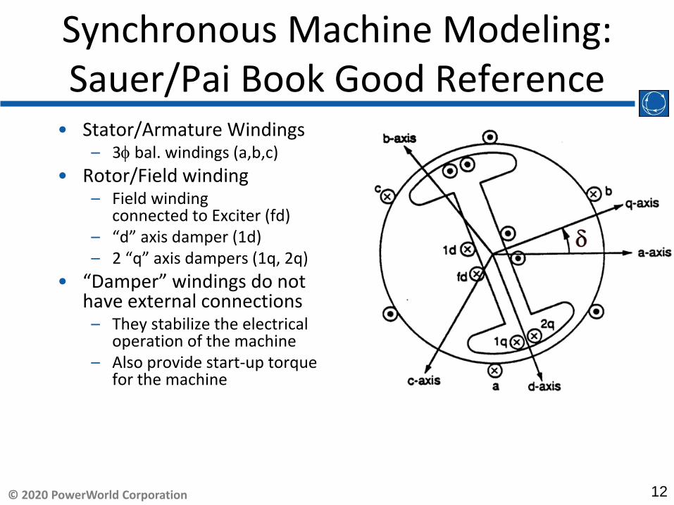
Synchronous Machine Modeling:Sauer/Pai Book Good Reference
• Stator/Armature Windings– 3φ bal. windings (a,b,c)
• Rotor/Field winding – Field winding
connected to Exciter (fd)– “d” axis damper (1d)– 2 “q” axis dampers (1q, 2q)
• “Damper” windings do not have external connections
– They stabilize the electrical operation of the machine
– Also provide start-up torque for the machine

13© 2020 PowerWorld Corporation
Dynamic Equations of a Synchronous Machine
• Start with Newton’s second law• Force = Mass * Acceleration• 𝐹𝐹 = 𝑀𝑀 𝑑𝑑𝑑𝑑
𝑑𝑑𝑑𝑑and 𝑑𝑑𝑥𝑥
𝑑𝑑𝑑𝑑= 𝑣𝑣
• We have a rotational system though, so instead we end up with something a little different
• Torque = Moment of Inertia * Angular Acceleration
• 𝑇𝑇 = 𝐽𝐽 𝑑𝑑𝜔𝜔𝑑𝑑𝑑𝑑
and 𝑑𝑑𝑑𝑑𝑑𝑑𝑑𝑑
= 𝜔𝜔
• Electrical Equations just apply the same equations to the circuits for the 7 windings a, b, c, fd, 1d, 1q, 2q
• 𝑣𝑣 = 𝑖𝑖𝑖𝑖 + 𝑑𝑑𝑑𝑑𝑑𝑑𝑑𝑑

14© 2020 PowerWorld Corporation
Fundamental Laws
• Kirchhoff’s Voltage Law, Ohm’s Law, Faraday’s Law, Newton’s Second Law
𝑣𝑣𝑓𝑓𝑑𝑑 = 𝑖𝑖𝑓𝑓𝑑𝑑𝑖𝑖𝑓𝑓𝑑𝑑 +𝑑𝑑𝜆𝜆𝑓𝑓𝑑𝑑
𝑑𝑑𝑑𝑑
𝑣𝑣1𝑑𝑑 = 𝑖𝑖1𝑑𝑑𝑖𝑖1𝑑𝑑 +𝑑𝑑𝜆𝜆1𝑑𝑑
𝑑𝑑𝑑𝑑
𝑣𝑣1𝑞𝑞 = 𝑖𝑖1𝑞𝑞𝑖𝑖1𝑞𝑞 +𝑑𝑑𝜆𝜆1𝑞𝑞
𝑑𝑑𝑑𝑑
𝑣𝑣2𝑞𝑞 = 𝑖𝑖2𝑞𝑞𝑖𝑖2𝑞𝑞 +𝑑𝑑𝜆𝜆2𝑞𝑞
𝑑𝑑𝑑𝑑
𝑣𝑣𝑎𝑎 = 𝑖𝑖𝑎𝑎𝑖𝑖𝑠𝑠 +𝑑𝑑𝜆𝜆𝑎𝑎
𝑑𝑑𝑑𝑑𝑣𝑣𝑏𝑏 = 𝑖𝑖𝑏𝑏𝑖𝑖𝑠𝑠 +
𝑑𝑑𝜆𝜆𝑏𝑏
𝑑𝑑𝑑𝑑𝑣𝑣𝑐𝑐 = 𝑖𝑖𝑐𝑐𝑖𝑖𝑠𝑠 +
𝑑𝑑𝜆𝜆𝑐𝑐
𝑑𝑑𝑑𝑑
𝑑𝑑𝜃𝜃shaft𝑑𝑑𝑑𝑑
=2𝑃𝑃
𝜔𝜔
𝐽𝐽2𝑃𝑃
𝑑𝑑𝜔𝜔𝑑𝑑𝑑𝑑
= 𝑇𝑇𝑚𝑚 − 𝑇𝑇𝑒𝑒 − 𝑇𝑇𝑓𝑓𝜔𝜔
Stator Rotor Shaft

15© 2020 PowerWorld Corporation
Deriving Equations for Rotor
• Algebra and trigonometry end up being extremely complex– Results give inductances between phases that are
a function of the cosine of rotor angle. Yuck!– Special transformations are done to transform the
abc phase quantities into another reference frame• Called the dq0 transformation
– Might hear it called “Park’s Transformation” after Robert H. Park who introduced this concept in 1929 (his was slightly scaled transformation, but was the same idea)
• Parks’ 1929 paper voted 2nd most important power paper of 20th century (1st was Fortescue’s sym. components)
• Convention used here is the q-axis leads the d-axis (which is the IEEE standard)

16© 2020 PowerWorld Corporation
dq0 Transformation
• This is a very similar idea as symmetrical components when discussing fault analysis (different matrix conversion though)
• We can say thanks to engineers who figured this all out for us 80 years ago!• We end up with 14 equations that go through conversion similar to following• Also make some more “magic” per unit choices to make things clean-up more
dq0

17© 2020 PowerWorld Corporation
Dq0 Transformations
1
or ,d a
q dqo b
co
a d
b dqo q
c o
v vv T v i
vv
v vv T vv v
λ
−
∆
=
In the next few slideswe’ll quickly go through how thesebasic equations aretransformed into thestandard machinemodels. The pointis to show the physicalbasis for the models.And there is NO quizat the end!!

18© 2020 PowerWorld Corporation
dq0 Transformations
2 2sin sin sin2 2 3 2 3
2 2 2cos cos cos3 2 2 3 2 3
1 1 12 2 2
shaft shaft shaft
dqo shaft shaft shaft
P P P
P P PT
π πθ θ θ
π πθ θ θ
− + ∆ − +
with the inverse,
+
+
−
−=−
13
22
cos3
22
sin
13
22
cos3
22
sin
12
cos2
sin
1
πθπθ
πθπθ
θθ
shaftshaft
shaftshaft
shaftshaft
dqo
PP
PP
PP
T
Note that thetransformationdepends on theshaft angle.
19© 2020 PowerWorld Corporation
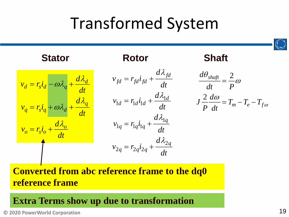
Transformed System
11 1 1
11 1 1
22 2 2
fdfd fd fd
dd d d
qq q q
qq q q
dv r i
dtdv r i
dtd
v r idtd
v r idt
λ
λ
λ
λ
= +
= +
= +
= +
2
2
shaft
m e f
ddt PdJ T T T
P dt ω
θω
ω
=
= − −
dd s d q
qq s q d
oo s o
dv r idt
dv r i
dtdv r idt
λωλ
λωλ
λ
= − +
= + +
= +
Stator Rotor Shaft
Converted from abc reference frame to the dq0 reference frame
Extra Terms show up due to transformation

20© 2020 PowerWorld Corporation
Electrical & Mechanical Relationships
Electrical system:
2
(voltage)
(power)
dv iRdt
dvi i R idt
λ
λ
= +
= +
Mechanical system:
2
2 (torque)
2 2 2 2 (power)
m e fw
m e fw
dJ T T TP dt
dJ T T TP dt P P P
ω
ωω ω ω ω
= − −
= − −
P is the number ofpoles (e.g. 2,4,6)
Mechanical Power
Electrical Torque
Friction and Windage

21© 2020 PowerWorld Corporation
Electric Torque Derivation
• Friction and Windage Torque: we ignore• Mechanical Torque: this is an input to the
system• Electrical Torque
– Torque is derived by looking at the overall energy balance in the system
– Three systems: electrical, mechanical and the coupling magnetic field
• Electrical system losses are in the form of resistance• Mechanical system losses are in the form of friction
– Coupling field is assumed to be lossless, hence we can track how energy moves between the electrical and mechanical systems

22© 2020 PowerWorld Corporation
Energy Conversion
No Losses in the Coupling Field

23© 2020 PowerWorld Corporation
Skip the Derivation
• A lot of interesting calculus and algebra using the “Conservative Coupling Field” assumption give us the electrical torque
• Also we define δ where 𝜔𝜔𝑠𝑠 is the synchronous speed
• This makes our mechanical equations
𝑇𝑇𝑒𝑒𝑒𝑒𝑒𝑒𝑐𝑐 = −32
𝑃𝑃2
𝜆𝜆𝑑𝑑𝐼𝐼𝑞𝑞 − 𝜆𝜆𝑞𝑞𝐼𝐼𝑑𝑑
2 shaft sP tδ θ ω∆ −
( )2 32 2
s
m d q q d f
ddt
d PJ T i i Tp dt ω
δ ω ω
ω λ λ
= −
= + − −

24© 2020 PowerWorld Corporation
Generator Swing Equation
• Anyway, after a lot of additional algebra, software tools model the swing equations as follows with values in per unit
– 2𝐻𝐻 𝑑𝑑𝜔𝜔𝑑𝑑t
= 𝑃𝑃𝑚𝑚𝑚𝑚𝑚𝑚𝑚1+𝜔𝜔
− 𝑇𝑇𝑒𝑒𝑒𝑒𝑒𝑒𝑐𝑐 and 𝑑𝑑𝑑𝑑𝑑𝑑𝑑𝑑
= 𝜔𝜔• If you use a more complete model of the rotor of a generator, then
the 𝑇𝑇𝑒𝑒𝑒𝑒𝑒𝑒𝑐𝑐 term has some inherent damping in it• In academic settings, as we’ll introduce in a moment, the rotor
modeling has no inherent damping in it (which makes your results really oscillate)
– To overcome this, folks in the 1960s added an extra 𝐷𝐷𝜔𝜔 term as follows
– This term should NOT be used to model the damping in the more accurate rotor models such as GENROU, GENSAL, GENTPF, GENTPJ, etc.
– Friction and Windage term has been removed for our purposes
2𝐻𝐻𝑑𝑑𝜔𝜔𝑑𝑑𝑑𝑑
=𝑃𝑃𝑚𝑚𝑒𝑒𝑐𝑐𝑚 − 𝐷𝐷𝜔𝜔
1 + 𝜔𝜔− 𝑇𝑇𝑒𝑒𝑒𝑒𝑒𝑒𝑐𝑐

25© 2020 PowerWorld Corporation
From here Lots of Per-Unit Choices
• Pages 30 – 42 in the Sauer/Pai textbook go through a ton of per unit scaling and lots of algebra
• Small notation differences, but we end up with the equations on the next page which largely match what Sauer/Pai derive – Different Notation though
(Our notation = Sauer/Pai)
• ψd′ = +ψ1𝑑𝑑
• ψ𝑞𝑞′ = −ψ2𝑞𝑞
Sauer/Pai Notation
Our Notation

26© 2020 PowerWorld Corporation
Variables and Constants
• Per Unit Model Variables– 𝜔𝜔𝑠𝑠 is the synchronous speed (2π60)– ∆𝜔𝜔𝑝𝑝𝑝𝑝 is the deviation of rotor speed away from synchronous
speed– 𝐼𝐼𝑑𝑑, 𝐼𝐼𝑞𝑞, 𝐼𝐼0 are the stator current in dq0 reference– 𝑉𝑉𝑑𝑑𝑑𝑑𝑒𝑒𝑑𝑑𝑚𝑚, 𝑉𝑉𝑞𝑞𝑑𝑑𝑒𝑒𝑑𝑑𝑚𝑚, 𝑉𝑉0𝑑𝑑𝑒𝑒𝑑𝑑𝑚𝑚 are the stator voltage in dq0 reference– ψ𝑑𝑑, ψ𝑞𝑞, ψ0 are the stator flux in the dq0 reference – 𝐸𝐸𝑑𝑑
′ , 𝐸𝐸𝑞𝑞′ , ψ𝑞𝑞
′ , and ψ𝑑𝑑′ represent per-unitized versions of the rotor
fluxes– 𝐸𝐸𝑓𝑓𝑑𝑑 is the field voltage input (from exciter)– 𝑃𝑃𝑚𝑚𝑒𝑒𝑐𝑐𝑚 is the mechanical power input (from turbine/governor)
• Per Unit Model Constants– 𝐻𝐻, 𝐷𝐷, 𝑅𝑅𝑠𝑠, 𝑋𝑋𝑑𝑑, 𝑋𝑋𝑑𝑑
′ , 𝑋𝑋𝑑𝑑′′, 𝑋𝑋𝑞𝑞, 𝑋𝑋𝑞𝑞
′ , 𝑋𝑋𝑞𝑞′′, 𝑋𝑋𝑒𝑒, 𝑇𝑇𝑑𝑑𝑑𝑑
′ , 𝑇𝑇𝑑𝑑𝑑𝑑′′ , 𝑇𝑇𝑞𝑞𝑑𝑑
′ , 𝑇𝑇𝑞𝑞𝑑𝑑′′

27© 2020 PowerWorld Corporation
Final Complete Model ofPer-Unitized Equations
2 Mechanical Dynamic Equations𝑑𝑑𝑑dt
= ∆𝜔𝜔𝑝𝑝𝑝𝑝 ∗ 𝜔𝜔𝑠𝑠
2𝐻𝐻 d𝜔𝜔𝑑𝑑𝑑𝑑
= 𝑃𝑃𝑚𝑚𝑚𝑚𝑚𝑚𝑚−𝐷𝐷𝜔𝜔1+∆𝜔𝜔𝑝𝑝𝑝𝑝
− ψ𝑑𝑑𝐼𝐼𝑞𝑞 − ψ𝑞𝑞𝐼𝐼𝑑𝑑
3 Stator Dynamic Equations1
𝜔𝜔𝑠𝑠
𝑑𝑑ψ𝑑𝑑𝑑𝑑𝑑𝑑
= 𝑅𝑅𝑠𝑠𝐼𝐼𝑑𝑑 + 1 + ∆𝜔𝜔𝑝𝑝𝑝𝑝 ψ𝑞𝑞 + 𝑉𝑉𝑑𝑑𝑑𝑑𝑒𝑒𝑑𝑑𝑚𝑚1
𝜔𝜔𝑠𝑠
𝑑𝑑ψ𝑞𝑞
𝑑𝑑𝑑𝑑= 𝑅𝑅𝑠𝑠𝐼𝐼𝑞𝑞 − 1 + ∆𝜔𝜔𝑝𝑝𝑝𝑝 ψ𝑑𝑑 + 𝑉𝑉𝑞𝑞𝑑𝑑𝑒𝑒𝑑𝑑𝑚𝑚
1𝜔𝜔𝑠𝑠
𝑑𝑑ψ0𝑑𝑑𝑑𝑑
= 𝑅𝑅𝑠𝑠𝐼𝐼0 + 𝑉𝑉0𝑑𝑑𝑒𝑒𝑑𝑑𝑚𝑚
4 Rotor Dynamic Equations
𝑇𝑇𝑑𝑑𝑑𝑑′ d𝐸𝐸𝑞𝑞
′
dt= 𝐸𝐸𝑓𝑓𝑑𝑑 − 𝐸𝐸𝑞𝑞
′ − 𝑋𝑋𝑑𝑑 − 𝑋𝑋𝑑𝑑′ 𝐼𝐼𝑑𝑑 − 𝑋𝑋𝑑𝑑
′ −𝑋𝑋𝑑𝑑′′
𝑋𝑋𝑑𝑑′ −𝑋𝑋𝑙𝑙
2 +ψ𝑑𝑑′ + 𝑋𝑋𝑑𝑑
′ − 𝑋𝑋𝑒𝑒 𝐼𝐼𝑑𝑑 − 𝐸𝐸𝑞𝑞′
𝑇𝑇𝑞𝑞𝑑𝑑′ d𝐸𝐸𝑑𝑑
′
dt= −𝐸𝐸𝑑𝑑
′ + 𝑋𝑋𝑞𝑞 − 𝑋𝑋𝑞𝑞′ 𝐼𝐼𝑞𝑞 − 𝑋𝑋𝑞𝑞
′ −𝑋𝑋𝑞𝑞′′
𝑋𝑋𝑞𝑞′ −𝑋𝑋𝑙𝑙
2 −ψ𝑞𝑞′ + 𝑋𝑋𝑞𝑞
′ − 𝑋𝑋𝑒𝑒 𝐼𝐼𝑞𝑞 + 𝐸𝐸𝑑𝑑′
𝑇𝑇𝑑𝑑𝑑𝑑′′ 𝑑𝑑ψd
′
dt= −ψ𝑑𝑑
′− 𝑋𝑋𝑑𝑑
′ − 𝑋𝑋𝑒𝑒 𝐼𝐼𝑑𝑑 + 𝐸𝐸𝑞𝑞′
𝑇𝑇𝑞𝑞𝑑𝑑′′ dψ𝑞𝑞
′
dt= −ψ𝑞𝑞
′ + 𝑋𝑋𝑞𝑞′ − 𝑋𝑋𝑒𝑒 𝐼𝐼𝑞𝑞 + 𝐸𝐸𝑑𝑑
′
Algebraic Relationship between Stator and Rotor Fluxesψ𝑑𝑑 = −𝐼𝐼𝑑𝑑𝑋𝑋𝑑𝑑
′′ + 𝐸𝐸𝑞𝑞′ 𝑋𝑋𝑑𝑑
′′−𝑋𝑋𝑙𝑙𝑋𝑋𝑑𝑑
′ −𝑋𝑋𝑙𝑙+ ψ𝑑𝑑
′ 𝑋𝑋𝑑𝑑′ −𝑋𝑋𝑑𝑑
′′
𝑋𝑋𝑑𝑑′ −𝑋𝑋𝑙𝑙
ψ𝑞𝑞 = −𝐼𝐼𝑞𝑞𝑋𝑋𝑞𝑞′′ − 𝐸𝐸𝑑𝑑
′ 𝑋𝑋𝑞𝑞′′−𝑋𝑋𝑙𝑙
𝑋𝑋𝑞𝑞′ −𝑋𝑋𝑙𝑙
− ψ𝑞𝑞′ 𝑋𝑋𝑞𝑞
′ −𝑋𝑋𝑞𝑞′′
𝑋𝑋𝑞𝑞′ −𝑋𝑋𝑙𝑙
The 3 stator equations define what are known as the stator transients.
28© 2020 PowerWorld Corporation
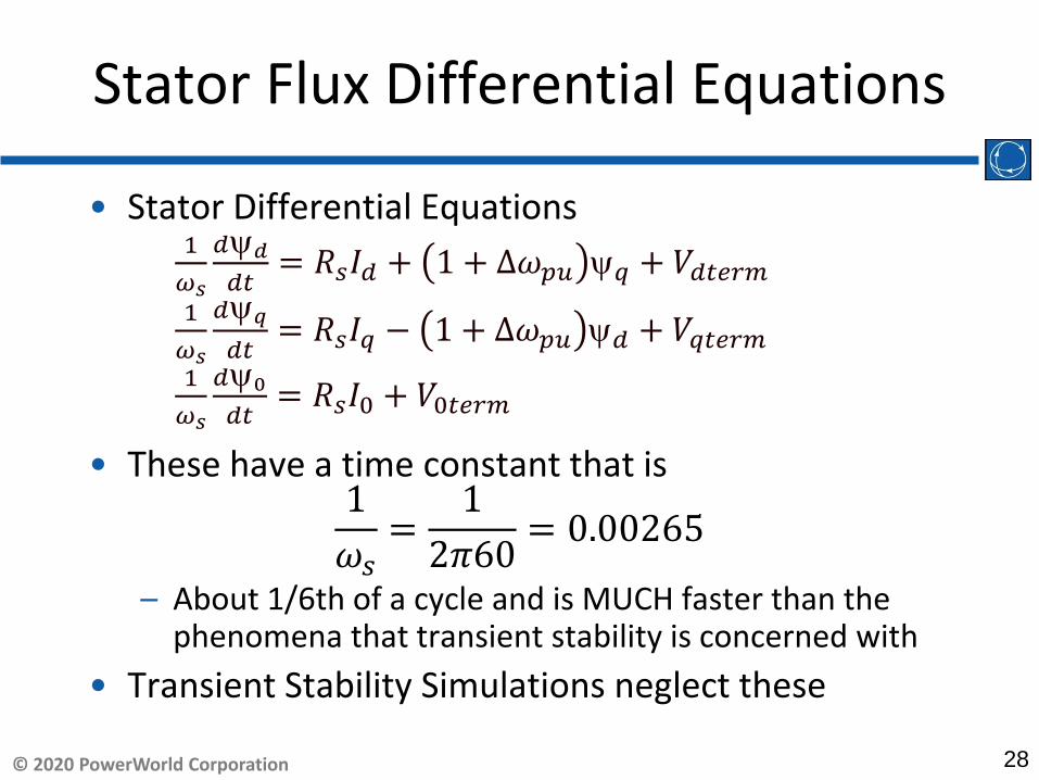
Stator Flux Differential Equations
• Stator Differential Equations
• These have a time constant that is 1
𝜔𝜔𝑠𝑠=
12𝜋𝜋𝜋𝜋
= 𝜋.𝜋𝜋2𝜋5
– About 1/6th of a cycle and is MUCH faster than the phenomena that transient stability is concerned with
• Transient Stability Simulations neglect these
1𝜔𝜔𝑠𝑠
𝑑𝑑ψ𝑑𝑑𝑑𝑑𝑑𝑑
= 𝑅𝑅𝑠𝑠𝐼𝐼𝑑𝑑 + 1 + ∆𝜔𝜔𝑝𝑝𝑝𝑝 ψ𝑞𝑞 + 𝑉𝑉𝑑𝑑𝑑𝑑𝑒𝑒𝑑𝑑𝑚𝑚1
𝜔𝜔𝑠𝑠
𝑑𝑑ψ𝑞𝑞
𝑑𝑑𝑑𝑑= 𝑅𝑅𝑠𝑠𝐼𝐼𝑞𝑞 − 1 + ∆𝜔𝜔𝑝𝑝𝑝𝑝 ψ𝑑𝑑 + 𝑉𝑉𝑞𝑞𝑑𝑑𝑒𝑒𝑑𝑑𝑚𝑚
1𝜔𝜔𝑠𝑠
𝑑𝑑ψ0𝑑𝑑𝑑𝑑
= 𝑅𝑅𝑠𝑠𝐼𝐼0 + 𝑉𝑉0𝑑𝑑𝑒𝑒𝑑𝑑𝑚𝑚
29© 2020 PowerWorld Corporation
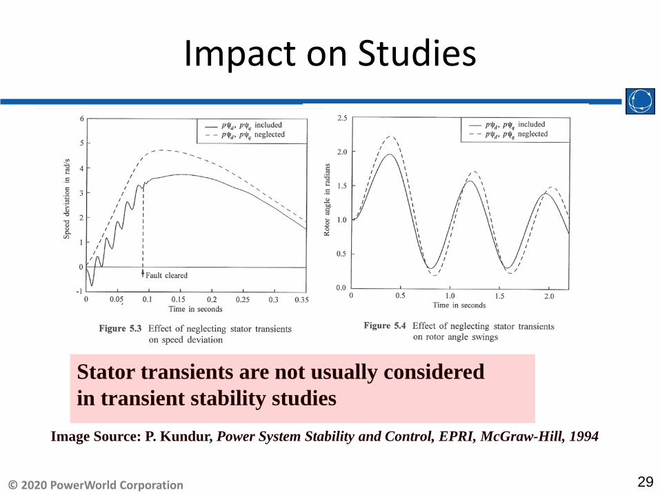
Impact on Studies
Image Source: P. Kundur, Power System Stability and Control, EPRI, McGraw-Hill, 1994
Stator transients are not usually considered in transient stability studies

30© 2020 PowerWorld Corporation
Elimination of Stator Transients
• Mathematics is kind of neat and you get to use terms like “Integral Manifold” and sound really smart
• Easier way to think of it – Regardless of what the derivative of these fluxes are,
they are multiplied by a very small number 1𝜔𝜔𝑠𝑠
and thus the left-hand side is near zero anyway, so approximation is made
1𝜔𝜔𝑠𝑠
𝑑𝑑ψ𝑑𝑑𝑑𝑑𝑑𝑑
≈ 𝜋 = 𝑅𝑅𝑠𝑠𝐼𝐼𝑑𝑑 + 1 + ∆𝜔𝜔𝑝𝑝𝑝𝑝 ψ𝑞𝑞 + 𝑉𝑉𝑑𝑑𝑑𝑑𝑒𝑒𝑑𝑑𝑚𝑚1
𝜔𝜔𝑠𝑠
𝑑𝑑ψ𝑞𝑞
𝑑𝑑𝑑𝑑≈ 𝜋 = 𝑅𝑅𝑠𝑠𝐼𝐼𝑞𝑞 − 1 + ∆𝜔𝜔𝑝𝑝𝑝𝑝 ψ𝑑𝑑 + 𝑉𝑉𝑞𝑞𝑑𝑑𝑒𝑒𝑑𝑑𝑚𝑚
1𝜔𝜔𝑠𝑠
𝑑𝑑ψ0𝑑𝑑𝑑𝑑
≈ 𝜋 = 𝑅𝑅𝑠𝑠𝐼𝐼0 + 𝑉𝑉0𝑑𝑑𝑒𝑒𝑑𝑑𝑚𝑚

31© 2020 PowerWorld Corporation
Stator Equations Becomes Algebraic Network Equation
• This gives us the following
• Take the algebraic flux relationship and plug it in
• Group Terms
𝑉𝑉𝑑𝑑𝑑𝑑𝑒𝑒𝑑𝑑𝑚𝑚 = −𝑅𝑅𝑠𝑠𝐼𝐼𝑑𝑑 − 1 + ∆𝜔𝜔𝑝𝑝𝑝𝑝 ψ𝑞𝑞𝑉𝑉𝑞𝑞𝑑𝑑𝑒𝑒𝑑𝑑𝑚𝑚 = −𝑅𝑅𝑠𝑠𝐼𝐼𝑞𝑞 + 1 + ∆𝜔𝜔𝑝𝑝𝑝𝑝 ψ𝑑𝑑
𝑉𝑉𝑑𝑑𝑑𝑑𝑒𝑒𝑑𝑑𝑚𝑚 = −𝑅𝑅𝑠𝑠𝐼𝐼𝑑𝑑 − 1 + ∆𝜔𝜔𝑝𝑝𝑝𝑝 −𝐼𝐼𝑞𝑞𝑋𝑋𝑞𝑞′′ − 𝐸𝐸𝑑𝑑
′ 𝑋𝑋𝑞𝑞′′−𝑋𝑋𝑙𝑙
𝑋𝑋𝑞𝑞′ −𝑋𝑋𝑙𝑙
− ψ𝑞𝑞′ 𝑋𝑋𝑞𝑞
′ −𝑋𝑋𝑞𝑞′′
𝑋𝑋𝑞𝑞′ −𝑋𝑋𝑙𝑙
𝑉𝑉𝑞𝑞𝑑𝑑𝑒𝑒𝑑𝑑𝑚𝑚 = −𝑅𝑅𝑠𝑠𝐼𝐼𝑞𝑞 + 1 + ∆𝜔𝜔𝑝𝑝𝑝𝑝 −𝐼𝐼𝑑𝑑𝑋𝑋𝑑𝑑′′ + 𝐸𝐸𝑞𝑞
′ 𝑋𝑋𝑑𝑑′′−𝑋𝑋𝑙𝑙
𝑋𝑋𝑑𝑑′ −𝑋𝑋𝑙𝑙
+ ψ𝑑𝑑′ 𝑋𝑋𝑑𝑑
′ −𝑋𝑋𝑑𝑑′′
𝑋𝑋𝑑𝑑′ −𝑋𝑋𝑙𝑙
𝑉𝑉𝑑𝑑𝑑𝑑𝑒𝑒𝑑𝑑𝑚𝑚 = −𝑅𝑅𝑠𝑠𝐼𝐼𝑑𝑑 + 1 + ∆𝜔𝜔𝑝𝑝𝑝𝑝 𝑋𝑋𝑞𝑞′′𝐼𝐼𝑞𝑞 + 1 + ∆𝜔𝜔𝑝𝑝𝑝𝑝 +𝐸𝐸𝑑𝑑
′ 𝑋𝑋𝑞𝑞′′−𝑋𝑋𝑙𝑙
𝑋𝑋𝑞𝑞′ −𝑋𝑋𝑙𝑙
+ ψ𝑞𝑞′ 𝑋𝑋𝑞𝑞
′ −𝑋𝑋𝑞𝑞′′
𝑋𝑋𝑞𝑞′ −𝑋𝑋𝑙𝑙
𝑉𝑉𝑞𝑞𝑑𝑑𝑒𝑒𝑑𝑑𝑚𝑚 = −𝑅𝑅𝑠𝑠𝐼𝐼𝑞𝑞 − 1 + ∆𝜔𝜔𝑝𝑝𝑝𝑝 𝑋𝑋𝑑𝑑′′𝐼𝐼𝑑𝑑 + 1 + ∆𝜔𝜔𝑝𝑝𝑝𝑝 +𝐸𝐸𝑞𝑞
′ 𝑋𝑋𝑑𝑑′′−𝑋𝑋𝑙𝑙
𝑋𝑋𝑑𝑑′ −𝑋𝑋𝑙𝑙
+ ψ𝑑𝑑′ 𝑋𝑋𝑑𝑑
′ −𝑋𝑋𝑑𝑑′′
𝑋𝑋𝑑𝑑′ −𝑋𝑋𝑙𝑙
Also remember stator flux relationshipsψ𝑑𝑑 = −𝐼𝐼𝑑𝑑𝑋𝑋𝑑𝑑
′′ + 𝐸𝐸𝑞𝑞′ 𝑋𝑋𝑑𝑑
′′−𝑋𝑋𝑙𝑙𝑋𝑋𝑑𝑑
′ −𝑋𝑋𝑙𝑙+ ψ𝑑𝑑
′ 𝑋𝑋𝑑𝑑′ −𝑋𝑋𝑑𝑑
′′
𝑋𝑋𝑑𝑑′ −𝑋𝑋𝑙𝑙
ψ𝑞𝑞 = −𝐼𝐼𝑞𝑞𝑋𝑋𝑞𝑞′′ − 𝐸𝐸𝑑𝑑
′ 𝑋𝑋𝑞𝑞′′−𝑋𝑋𝑙𝑙
𝑋𝑋𝑞𝑞′ −𝑋𝑋𝑙𝑙
− ψ𝑞𝑞′ 𝑋𝑋𝑞𝑞
′ −𝑋𝑋𝑞𝑞′′
𝑋𝑋𝑞𝑞′ −𝑋𝑋𝑙𝑙

32© 2020 PowerWorld Corporation
Stator Equation Becomes Network Equation
• Now define
• This gives us the following
• Consider term 1 + ∆𝜔𝜔𝑝𝑝𝑝𝑝 that remains– Similar to multiplying all the transmission line X values by per unit
frequency to scale the network impedances as system frequency changes
• No one does this in transient stability, so we just remove the purple• We leave the scaling of the internal voltage though
𝑉𝑉𝑑𝑑𝑑𝑑𝑒𝑒𝑑𝑑𝑚𝑚 = −𝑅𝑅𝑠𝑠𝐼𝐼𝑑𝑑 + 1 + ∆𝜔𝜔𝑝𝑝𝑝𝑝 𝑋𝑋𝑑𝑑′′𝐼𝐼𝑞𝑞 + 𝐸𝐸𝑑𝑑
′′ 1 + ∆𝜔𝜔𝑝𝑝𝑝𝑝𝑉𝑉𝑞𝑞𝑑𝑑𝑒𝑒𝑑𝑑𝑚𝑚 = −𝑅𝑅𝑠𝑠𝐼𝐼𝑞𝑞 − 1 + ∆𝜔𝜔𝑝𝑝𝑝𝑝 𝑋𝑋𝑑𝑑
′′𝐼𝐼𝑑𝑑 + 𝐸𝐸𝑞𝑞′′ 1 + ∆𝜔𝜔𝑝𝑝𝑝𝑝
𝐸𝐸𝑑𝑑′′ = +𝐸𝐸𝑑𝑑
′ 𝑋𝑋𝑞𝑞′′−𝑋𝑋𝑙𝑙
𝑋𝑋𝑞𝑞′ −𝑋𝑋𝑙𝑙
+ ψ𝑞𝑞′ 𝑋𝑋𝑞𝑞
′ −𝑋𝑋𝑞𝑞′′
𝑋𝑋𝑞𝑞′ −𝑋𝑋𝑙𝑙
𝐸𝐸𝑞𝑞′′ = +𝐸𝐸𝑞𝑞
′ 𝑋𝑋𝑑𝑑′′−𝑋𝑋𝑙𝑙
𝑋𝑋𝑑𝑑′ −𝑋𝑋𝑙𝑙
+ ψ𝑑𝑑′ 𝑋𝑋𝑑𝑑
′ −𝑋𝑋𝑑𝑑′′
𝑋𝑋𝑑𝑑′ −𝑋𝑋𝑙𝑙
𝑉𝑉𝑑𝑑𝑑𝑑𝑒𝑒𝑑𝑑𝑚𝑚 = 𝐸𝐸𝑑𝑑′′ 1 + ∆𝜔𝜔𝑝𝑝𝑝𝑝 − 𝑅𝑅𝑠𝑠𝐼𝐼𝑑𝑑 + 𝑋𝑋𝑞𝑞
′′𝐼𝐼𝑞𝑞𝑉𝑉𝑞𝑞𝑑𝑑𝑒𝑒𝑑𝑑𝑚𝑚 = 𝐸𝐸𝑞𝑞
′′ 1 + ∆𝜔𝜔𝑝𝑝𝑝𝑝 − 𝑅𝑅𝑠𝑠𝐼𝐼𝑞𝑞 − 𝑋𝑋𝑑𝑑′′𝐼𝐼𝑑𝑑

33© 2020 PowerWorld Corporation
Final Complete Model ofPer-Unitized Equations
6 Differential Equations1. 𝑑𝑑𝑑
dt= ∆𝜔𝜔𝑝𝑝𝑝𝑝 ∗ 𝜔𝜔𝑠𝑠
2. 2𝐻𝐻 d𝜔𝜔𝑑𝑑𝑑𝑑
= 𝑃𝑃𝑚𝑚𝑚𝑚𝑚𝑚𝑚−𝐷𝐷𝜔𝜔1+∆𝜔𝜔𝑝𝑝𝑝𝑝
− ψ𝑑𝑑𝐼𝐼𝑞𝑞 − ψ𝑞𝑞𝐼𝐼𝑑𝑑
3. 𝑇𝑇𝑑𝑑𝑑𝑑′ d𝐸𝐸𝑞𝑞
′
dt= 𝐸𝐸𝑓𝑓𝑑𝑑 − 𝐸𝐸𝑞𝑞
′ − 𝑋𝑋𝑑𝑑 − 𝑋𝑋𝑑𝑑′ 𝐼𝐼𝑑𝑑 − 𝑋𝑋𝑑𝑑
′ −𝑋𝑋𝑑𝑑′′
𝑋𝑋𝑑𝑑′ −𝑋𝑋𝑙𝑙
2 +ψ𝑑𝑑′ + 𝑋𝑋𝑑𝑑
′ − 𝑋𝑋𝑒𝑒 𝐼𝐼𝑑𝑑 − 𝐸𝐸𝑞𝑞′
4. 𝑇𝑇𝑞𝑞𝑑𝑑′ d𝐸𝐸𝑑𝑑
′
dt= −𝐸𝐸𝑑𝑑
′ + 𝑋𝑋𝑞𝑞 − 𝑋𝑋𝑞𝑞′ 𝐼𝐼𝑞𝑞 − 𝑋𝑋𝑞𝑞
′ −𝑋𝑋𝑞𝑞′′
𝑋𝑋𝑞𝑞′ −𝑋𝑋𝑙𝑙
2 −ψ𝑞𝑞′ + 𝑋𝑋𝑞𝑞
′ − 𝑋𝑋𝑒𝑒 𝐼𝐼𝑞𝑞 + 𝐸𝐸𝑑𝑑′
5. 𝑇𝑇𝑑𝑑𝑑𝑑′′ 𝑑𝑑ψd
′
dt= −ψ𝑑𝑑
′− 𝑋𝑋𝑑𝑑
′ − 𝑋𝑋𝑒𝑒 𝐼𝐼𝑑𝑑 + 𝐸𝐸𝑞𝑞′
𝜋. 𝑇𝑇𝑞𝑞𝑑𝑑′′ dψ𝑞𝑞
′
dt= −ψ𝑞𝑞
′ + 𝑋𝑋𝑞𝑞′ − 𝑋𝑋𝑒𝑒 𝐼𝐼𝑞𝑞 + 𝐸𝐸𝑑𝑑
′
Algebraic Relationships𝐸𝐸𝑑𝑑
′′ = +𝐸𝐸𝑑𝑑′ 𝑋𝑋𝑞𝑞
′′−𝑋𝑋𝑙𝑙
𝑋𝑋𝑞𝑞′ −𝑋𝑋𝑙𝑙
+ ψ𝑞𝑞′ 𝑋𝑋𝑞𝑞
′ −𝑋𝑋𝑞𝑞′′
𝑋𝑋𝑞𝑞′ −𝑋𝑋𝑙𝑙
𝐸𝐸𝑞𝑞′′ = +𝐸𝐸𝑞𝑞
′ 𝑋𝑋𝑑𝑑′′−𝑋𝑋𝑙𝑙
𝑋𝑋𝑑𝑑′ −𝑋𝑋𝑙𝑙
+ ψ𝑑𝑑′ 𝑋𝑋𝑑𝑑
′ −𝑋𝑋𝑑𝑑′′
𝑋𝑋𝑑𝑑′ −𝑋𝑋𝑙𝑙
ψ𝑑𝑑 = −𝐼𝐼𝑑𝑑𝑋𝑋𝑑𝑑′′ + 𝐸𝐸𝑞𝑞
′′
ψ𝑞𝑞 = −𝐼𝐼𝑞𝑞𝑋𝑋𝑑𝑑′′ − 𝐸𝐸𝑑𝑑
′′
𝑉𝑉𝑑𝑑𝑑𝑑𝑒𝑒𝑑𝑑𝑚𝑚 = 𝐸𝐸𝑑𝑑′′ 1 + ∆𝜔𝜔𝑝𝑝𝑝𝑝 − 𝑅𝑅𝑠𝑠𝐼𝐼𝑑𝑑 + 𝑋𝑋𝑞𝑞
′′𝐼𝐼𝑞𝑞𝑉𝑉𝑞𝑞𝑑𝑑𝑒𝑒𝑑𝑑𝑚𝑚 = 𝐸𝐸𝑞𝑞
′′ 1 + ∆𝜔𝜔𝑝𝑝𝑝𝑝 − 𝑅𝑅𝑠𝑠𝐼𝐼𝑞𝑞 − 𝑋𝑋𝑑𝑑′′𝐼𝐼𝑑𝑑

34© 2020 PowerWorld Corporation
Field Voltage and Current
• Field Voltage (𝐸𝐸𝑓𝑓𝑑𝑑) is an input from the exciter• The field current, 𝐼𝐼𝑓𝑓𝑑𝑑, is defined in steady-state as
• Traditional, when we talk about a “field current” we are actually mean the product of the field current and the mutual inductance 𝐼𝐼𝑓𝑓𝑑𝑑𝑋𝑋𝑚𝑚𝑑𝑑 (also written 𝐼𝐼𝑓𝑓𝑑𝑑𝐿𝐿𝑎𝑎𝑑𝑑)
𝐼𝐼𝑓𝑓𝑑𝑑 = 𝐸𝐸𝑓𝑓𝑑𝑑/𝑋𝑋𝑚𝑚𝑑𝑑
𝐿𝐿𝑎𝑎𝑑𝑑𝐼𝐼𝑓𝑓𝑑𝑑 = 𝐸𝐸𝑞𝑞′ + 𝑋𝑋𝑑𝑑 − 𝑋𝑋𝑑𝑑
′ 𝐼𝐼𝑑𝑑 − 𝑋𝑋𝑑𝑑′ −𝑋𝑋𝑑𝑑
′′
𝑋𝑋𝑑𝑑′ −𝑋𝑋𝑙𝑙
2 +ψ𝑑𝑑′ + 𝑋𝑋𝑑𝑑
′ − 𝑋𝑋𝑒𝑒 𝐼𝐼𝑑𝑑 − 𝐸𝐸𝑞𝑞′
𝑇𝑇𝑑𝑑𝑑𝑑′ d𝐸𝐸𝑞𝑞
′
dt= 𝐸𝐸𝑓𝑓𝑑𝑑 − 𝐿𝐿𝑎𝑎𝑑𝑑𝐼𝐼𝑓𝑓𝑑𝑑

35© 2020 PowerWorld Corporation
Multiple Machines
• This math is all very beautiful, but it is all related to a single machine that is connected to a three-phase system
• We need a similar conversion for the abcquantities at all the network buses
• This requires us to do some more beautiful math
• We will first convert all network abcquantities to a common reference frame we call the Synchronous Reference Frame

36© 2020 PowerWorld Corporation
Synchronously Rotating Reference Frame
• That conversion is chosen as follows– It was chosen because the math works out so nicely
• Assume you have a 3-phase balanced voltage
𝑇𝑇𝑠𝑠𝑠𝑠𝑠𝑠𝑐𝑐 =23
cos 𝜔𝜔𝑑𝑑 cos 𝜔𝜔𝑑𝑑 −2𝜋𝜋3
cos 𝜔𝜔𝑑𝑑 +2𝜋𝜋3
−sin 𝜔𝜔𝑑𝑑 −sin 𝜔𝜔𝑑𝑑 −2𝜋𝜋3
− sin 𝜔𝜔𝑑𝑑 +2𝜋𝜋3
1/2 1/2 1/2
𝑣𝑣𝐷𝐷𝑣𝑣𝑄𝑄𝑣𝑣𝑂𝑂
= 𝑇𝑇𝑠𝑠𝑠𝑠𝑠𝑠𝑐𝑐
𝑉𝑉𝑎𝑎𝑉𝑉𝑏𝑏𝑉𝑉𝑐𝑐
𝑣𝑣𝐷𝐷𝑣𝑣𝑄𝑄𝑣𝑣𝑂𝑂
=23
cos 𝜔𝜔𝑑𝑑 cos 𝜔𝜔𝑑𝑑 −2𝜋𝜋3
cos 𝜔𝜔𝑑𝑑 +2𝜋𝜋3
−sin 𝜔𝜔𝑑𝑑 −sin 𝜔𝜔𝑑𝑑 −2𝜋𝜋3
− sin 𝜔𝜔𝑑𝑑 +2𝜋𝜋3
1/2 1/2 1/2
𝑉𝑉𝑑𝑑 cos 𝜔𝜔𝑑𝑑 + 𝛼𝛼
𝑉𝑉𝑑𝑑 cos 𝜔𝜔𝑑𝑑 + 𝛼𝛼 −2𝜋𝜋3
𝑉𝑉𝑑𝑑 cos 𝜔𝜔𝑑𝑑 + 𝛼𝛼 +2𝜋𝜋3
37© 2020 PowerWorld Corporation
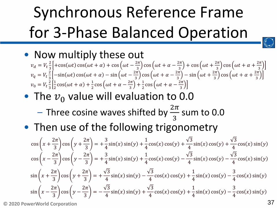
Synchronous Reference Frame for 3-Phase Balanced Operation
• Now multiply these out
• The 𝑣𝑣0 value will evaluation to 0.0– Three cosine waves shifted by 2𝜋𝜋
3sum to 0.0
• Then use of the following trigonometry
𝑣𝑣𝑑𝑑 = 𝑉𝑉𝑑𝑑23
+cos 𝜔𝜔𝑑𝑑 cos 𝜔𝜔𝑑𝑑 + 𝛼𝛼 + cos 𝜔𝜔𝑑𝑑 − 2𝜋𝜋3
cos 𝜔𝜔𝑑𝑑 + 𝛼𝛼 − 2𝜋𝜋3
+ cos 𝜔𝜔𝑑𝑑 + 2𝜋𝜋3
cos 𝜔𝜔𝑑𝑑 + 𝛼𝛼 + 2𝜋𝜋3
𝑣𝑣𝑞𝑞 = 𝑉𝑉𝑑𝑑23
−sin 𝜔𝜔𝑑𝑑 cos 𝜔𝜔𝑑𝑑 + 𝛼𝛼 − sin 𝜔𝜔𝑑𝑑 − 2𝜋𝜋3
cos 𝜔𝜔𝑑𝑑 + 𝛼𝛼 − 2𝜋𝜋3
− sin 𝜔𝜔𝑑𝑑 + 2𝜋𝜋3
cos 𝜔𝜔𝑑𝑑 + 𝛼𝛼 + 2𝜋𝜋3
𝑣𝑣0 = 𝑉𝑉𝑑𝑑23
12
cos 𝜔𝜔𝑑𝑑 + 𝛼𝛼 + 12
cos 𝜔𝜔𝑑𝑑 + 𝛼𝛼 − 2𝜋𝜋3
+ 12
cos 𝜔𝜔𝑑𝑑 + 𝛼𝛼 − 2𝜋𝜋3
cos 𝑥𝑥 +2𝜋𝜋3
cos 𝑦𝑦 +2𝜋𝜋3
= +34
sin 𝑥𝑥 sin 𝑦𝑦 +14
cos 𝑥𝑥 cos 𝑦𝑦 +3
4sin 𝑥𝑥 cos 𝑦𝑦 +
34
cos 𝑥𝑥 sin 𝑦𝑦
cos 𝑥𝑥 −2𝜋𝜋3
cos 𝑦𝑦 −2𝜋𝜋3
= +34
sin 𝑥𝑥 sin 𝑦𝑦 +14
cos 𝑥𝑥 cos 𝑦𝑦 −3
4sin 𝑥𝑥 cos 𝑦𝑦 −
34
cos 𝑥𝑥 sin 𝑦𝑦
sin 𝑥𝑥 +2𝜋𝜋3
cos 𝑦𝑦 +2𝜋𝜋3
= +3
4sin 𝑥𝑥 sin 𝑦𝑦 −
34
cos 𝑥𝑥 cos 𝑦𝑦 +14
sin 𝑥𝑥 cos 𝑦𝑦 −34
cos 𝑥𝑥 sin 𝑦𝑦
sin 𝑥𝑥 −2𝜋𝜋3
cos 𝑦𝑦 −2𝜋𝜋3
= −3
4sin 𝑥𝑥 sin 𝑦𝑦 +
34
cos 𝑥𝑥 cos 𝑦𝑦 +14
sin 𝑥𝑥 cos 𝑦𝑦 −34
cos 𝑥𝑥 sin 𝑦𝑦
38© 2020 PowerWorld Corporation
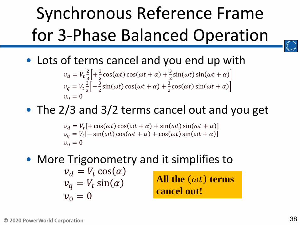
Synchronous Reference Frame for 3-Phase Balanced Operation
• Lots of terms cancel and you end up with
• The 2/3 and 3/2 terms cancel out and you get
• More Trigonometry and it simplifies to
𝑣𝑣𝑑𝑑 = 𝑉𝑉𝑑𝑑23
+ 32
cos 𝜔𝜔𝑑𝑑 cos 𝜔𝜔𝑑𝑑 + 𝛼𝛼 + 32
sin 𝜔𝜔𝑑𝑑 sin 𝜔𝜔𝑑𝑑 + 𝛼𝛼
𝑣𝑣𝑞𝑞 = 𝑉𝑉𝑑𝑑23
− 32
sin 𝜔𝜔𝑑𝑑 cos 𝜔𝜔𝑑𝑑 + 𝛼𝛼 + 32
cos 𝜔𝜔𝑑𝑑 sin 𝜔𝜔𝑑𝑑 + 𝛼𝛼𝑣𝑣0 = 𝜋
𝑣𝑣𝑑𝑑 = 𝑉𝑉𝑑𝑑 + cos 𝜔𝜔𝑑𝑑 cos 𝜔𝜔𝑑𝑑 + 𝛼𝛼 + sin 𝜔𝜔𝑑𝑑 sin 𝜔𝜔𝑑𝑑 + 𝛼𝛼𝑣𝑣𝑞𝑞 = 𝑉𝑉𝑑𝑑 − sin 𝜔𝜔𝑑𝑑 cos 𝜔𝜔𝑑𝑑 + 𝛼𝛼 + cos 𝜔𝜔𝑑𝑑 sin 𝜔𝜔𝑑𝑑 + 𝛼𝛼𝑣𝑣0 = 𝜋
𝑣𝑣𝑑𝑑 = 𝑉𝑉𝑑𝑑 cos 𝛼𝛼𝑣𝑣𝑞𝑞 = 𝑉𝑉𝑑𝑑 sin 𝛼𝛼𝑣𝑣0 = 𝜋
All the 𝜔𝜔𝑑𝑑 terms cancel out!

39© 2020 PowerWorld Corporation
Synchronous Reference Frame for 3-Phase Balanced Operation
• A-phase sinusoidal is 𝑉𝑉𝑑𝑑 cos 𝜔𝜔𝑑𝑑 + 𝛼𝛼– Magnitude of 𝑉𝑉𝑑𝑑 and phase difference from the
“synchronous reference frame” of 𝛼𝛼• Value converted to the
synchronous reference frame are
• That means we can treat this like a complex number and just jump right to
• This is exactly what we always do in steady state power flow equations, so this is nothing new!
𝑣𝑣𝐷𝐷𝑣𝑣𝑄𝑄𝑣𝑣𝑂𝑂
=+𝑉𝑉𝑑𝑑 cos 𝛼𝛼+𝑉𝑉𝑑𝑑 sin 𝛼𝛼
𝜋
𝑣𝑣𝐷𝐷 + 𝑗𝑗𝑣𝑣𝑄𝑄 = 𝑉𝑉𝑑𝑑 cos 𝛼𝛼 + 𝑗𝑗𝑉𝑉𝑑𝑑 sin 𝛼𝛼 = 𝑉𝑉𝑑𝑑𝑒𝑒𝑗𝑗𝛼𝛼

40© 2020 PowerWorld Corporation
Must Apply Same Synchronous Reference Frame to Machine
• Remember that the abc quantities are converted to the machine reference frame.
• We then need to additionally transform those to the Network Reference
• Need the matrix in yellow for direct conversion• “Synchronous Reference Frame" Just call it the “Network Reference”– Network Reference Frame– Machine Reference Frame
𝑣𝑣𝐷𝐷𝑣𝑣𝑄𝑄𝑣𝑣𝑂𝑂
= 𝑇𝑇𝑠𝑠𝑠𝑠𝑠𝑠𝑐𝑐
𝑉𝑉𝑎𝑎𝑉𝑉𝑏𝑏𝑉𝑉𝑐𝑐
= 𝑇𝑇𝑠𝑠𝑠𝑠𝑠𝑠𝑐𝑐𝑇𝑇𝑑𝑑𝑞𝑞𝑑𝑑𝑑𝑑−1
𝑉𝑉𝑑𝑑𝑑𝑑𝑉𝑉𝑞𝑞𝑑𝑑𝑉𝑉0𝑑𝑑
𝑉𝑉𝑎𝑎𝑉𝑉𝑏𝑏𝑉𝑉𝑐𝑐
= 𝑇𝑇𝑑𝑑𝑞𝑞𝑑𝑑𝑑𝑑−1
𝑉𝑉𝑑𝑑𝑑𝑑𝑉𝑉𝑞𝑞𝑑𝑑𝑉𝑉0𝑑𝑑
𝑣𝑣𝐷𝐷𝑣𝑣𝑄𝑄𝑣𝑣𝑂𝑂
= 𝑇𝑇𝑠𝑠𝑠𝑠𝑠𝑠𝑐𝑐𝑇𝑇𝑑𝑑𝑞𝑞𝑑𝑑𝑑𝑑−1
𝑉𝑉𝑑𝑑𝑑𝑑𝑉𝑉𝑞𝑞𝑑𝑑𝑉𝑉0𝑑𝑑

41© 2020 PowerWorld Corporation
Converting Machine to Network Reference Frame
• Remember how we converted the abc phase stator quantities to the dq0 reference frame
• Also remember our choice of
• Thus 𝑃𝑃2
𝜃𝜃𝑠𝑠𝑚𝑎𝑎𝑓𝑓𝑑𝑑 = 𝜔𝜔𝑠𝑠𝑑𝑑 + 𝛿𝛿2 shaft sP tδ θ ω∆ −
+
+
−
−=−
13
22
cos3
22
sin
13
22
cos3
22
sin
12
cos2
sin
1
πθπθ
πθπθ
θθ
shaftshaft
shaftshaft
shaftshaft
dqo
PP
PP
PP
T

42© 2020 PowerWorld Corporation
Converting Machine to Network Reference Frame
• This makes our transformation matrix for a particular machine “i” the following
• This means for our machine reference frame to network reference frame we need the following
𝑇𝑇𝑑𝑑𝑞𝑞0𝑑𝑑−1 =
sin 𝜔𝜔𝑑𝑑 + 𝛿𝛿 cos 𝜔𝜔𝑑𝑑 + 𝛿𝛿 1
sin 𝜔𝜔𝑑𝑑 + 𝛿𝛿 −2𝜋𝜋3
cos 𝜔𝜔𝑑𝑑 + 𝛿𝛿 −2𝜋𝜋3
1
sin 𝜔𝜔𝑑𝑑 + 𝛿𝛿 +2𝜋𝜋3
cos 𝜔𝜔𝑑𝑑 + 𝛿𝛿 +2𝜋𝜋3
1
𝑇𝑇𝑠𝑠𝑠𝑠𝑠𝑠𝑐𝑐𝑇𝑇𝑑𝑑𝑞𝑞0−1 = 2
3
cos 𝜔𝜔𝑑𝑑 cos 𝜔𝜔𝑑𝑑 − 2𝜋𝜋3
cos 𝜔𝜔𝑑𝑑 + 2𝜋𝜋3
−sin 𝜔𝜔𝑑𝑑 −sin 𝜔𝜔𝑑𝑑 − 2𝜋𝜋3
− sin 𝜔𝜔𝑑𝑑 + 2𝜋𝜋3
1/2 1/2 1/2
sin 𝜔𝜔𝑑𝑑 + 𝛿𝛿 cos 𝜔𝜔𝑑𝑑 + 𝛿𝛿 1sin 𝜔𝜔𝑑𝑑 + 𝛿𝛿 − 2𝜋𝜋
3cos 𝜔𝜔𝑑𝑑 + 𝛿𝛿 − 2𝜋𝜋
31
sin 𝜔𝜔𝑑𝑑 + 𝛿𝛿 + 2𝜋𝜋3
cos 𝜔𝜔𝑑𝑑 + 𝛿𝛿 + 2𝜋𝜋3
1

43© 2020 PowerWorld Corporation
Converting Machine to Network Reference Frame
• Use the trigonometry identities
• When you group terms all the cos 2𝑥𝑥 + 𝛿𝛿and sin 2𝑥𝑥 + 𝛿𝛿 terms are going to cancel out and you only have the
𝑇𝑇𝑠𝑠𝑠𝑠𝑠𝑠𝑐𝑐𝑇𝑇𝑑𝑑𝑞𝑞0−1 = 2
3
cos 𝜔𝜔𝑑𝑑 cos 𝜔𝜔𝑑𝑑 − 2𝜋𝜋3
cos 𝜔𝜔𝑑𝑑 + 2𝜋𝜋3
−sin 𝜔𝜔𝑑𝑑 −sin 𝜔𝜔𝑑𝑑 − 2𝜋𝜋3
− sin 𝜔𝜔𝑑𝑑 + 2𝜋𝜋3
1/2 1/2 1/2
sin 𝜔𝜔𝑑𝑑 + 𝛿𝛿 cos 𝜔𝜔𝑑𝑑 + 𝛿𝛿 1sin 𝜔𝜔𝑑𝑑 + 𝛿𝛿 − 2𝜋𝜋
3cos 𝜔𝜔𝑑𝑑 + 𝛿𝛿 − 2𝜋𝜋
31
sin 𝜔𝜔𝑑𝑑 + 𝛿𝛿 + 2𝜋𝜋3
cos 𝜔𝜔𝑑𝑑 + 𝛿𝛿 + 2𝜋𝜋3
1
− sin 𝑥𝑥 sin 𝑥𝑥 + 𝛿𝛿 = − 12
cos 𝛿𝛿 + 12
cos 2𝑥𝑥 + 𝛿𝛿
− sin 𝑥𝑥 cos 𝑥𝑥 + 𝛿𝛿 = + 12
sin 𝛿𝛿 − 12
sin 2𝑥𝑥 + 𝛿𝛿
+ cos 𝑥𝑥 cos 𝑥𝑥 + 𝛿𝛿 = + 12
cos 𝛿𝛿 + 12
cos 2𝑥𝑥 + 𝛿𝛿
+ cos 𝑥𝑥 sin 𝑥𝑥 + 𝛿𝛿 = + 12
sin 𝛿𝛿 + 12
sin 2𝑥𝑥 + 𝛿𝛿
𝑇𝑇𝑠𝑠𝑠𝑠𝑠𝑠𝑐𝑐𝑇𝑇𝑑𝑑𝑞𝑞0−1 = 2
3
+ 32
sin 𝛿𝛿 + 32
cos 𝛿𝛿 𝜋
− 32
cos 𝛿𝛿 + 32
sin 𝛿𝛿 𝜋𝜋 𝜋 1
All the 𝜔𝜔𝑑𝑑 terms cancel out!

44© 2020 PowerWorld Corporation
Converting Machine to Network Reference Frame
• Thus the conversion from Machine Network is
• And the conversion from Network Machine is
𝑇𝑇𝑠𝑠𝑠𝑠𝑠𝑠𝑐𝑐𝑇𝑇𝑑𝑑𝑞𝑞0−1 =
+sin 𝛿𝛿 +cos 𝛿𝛿 𝜋−cos 𝛿𝛿 +sin 𝛿𝛿 𝜋
𝜋 𝜋 1
𝑇𝑇𝑑𝑑𝑞𝑞0𝑇𝑇𝑠𝑠𝑠𝑠𝑠𝑠𝑐𝑐−1 =
+sin 𝛿𝛿 −cos 𝛿𝛿 𝜋+cos 𝛿𝛿 +sin 𝛿𝛿 𝜋
𝜋 𝜋 1

45© 2020 PowerWorld Corporation
Various Reference Conversions
Synchronous ReferenceFrame
Machine (Rotor) Reference Frame
ABC phase Reference
23
cos 𝜔𝜔𝑑𝑑 cos 𝜔𝜔𝑑𝑑 −2𝜋𝜋3 cos 𝜔𝜔𝑑𝑑 +
2𝜋𝜋3
−sin 𝜔𝜔𝑑𝑑 −sin 𝜔𝜔𝑑𝑑 −2𝜋𝜋3 − sin 𝜔𝜔𝑑𝑑 +
2𝜋𝜋3
1/2 1/2 1/2
sin 𝜔𝜔𝑑𝑑 + 𝛿𝛿 cos 𝜔𝜔𝑑𝑑 + 𝛿𝛿 1
sin 𝜔𝜔𝑑𝑑 + 𝛿𝛿 −2𝜋𝜋3
cos 𝜔𝜔𝑑𝑑 + 𝛿𝛿 −2𝜋𝜋3
1
sin 𝜔𝜔𝑑𝑑 + 𝛿𝛿 +2𝜋𝜋3
cos 𝜔𝜔𝑑𝑑 + 𝛿𝛿 +2𝜋𝜋3
1
𝑇𝑇𝑠𝑠𝑠𝑠𝑠𝑠𝑐𝑐𝑇𝑇𝑑𝑑𝑞𝑞0−1
+sin 𝛿𝛿 +cos 𝛿𝛿 𝜋−cos 𝛿𝛿 +sin 𝛿𝛿 𝜋
𝜋 𝜋 1𝑇𝑇𝑠𝑠𝑠𝑠𝑠𝑠𝑐𝑐𝑇𝑇𝑑𝑑𝑞𝑞0
−1

46© 2020 PowerWorld Corporation
We shall never speak of the ABC Phase Reference Again!
Synchronous ReferenceFrame
Machine (Rotor) Reference Frame
ABC phase Reference
+sin 𝛿𝛿 +cos 𝛿𝛿 𝜋−cos 𝛿𝛿 +sin 𝛿𝛿 𝜋
𝜋 𝜋 1
23
cos 𝜔𝜔𝑑𝑑 cos 𝜔𝜔𝑑𝑑 −2𝜋𝜋3 cos 𝜔𝜔𝑑𝑑 +
2𝜋𝜋3
−sin 𝜔𝜔𝑑𝑑 −sin 𝜔𝜔𝑑𝑑 −2𝜋𝜋3 − sin 𝜔𝜔𝑑𝑑 +
2𝜋𝜋3
1/2 1/2 1/2
sin 𝜔𝜔𝑑𝑑 + 𝛿𝛿 cos 𝜔𝜔𝑑𝑑 + 𝛿𝛿 1
sin 𝜔𝜔𝑑𝑑 + 𝛿𝛿 −2𝜋𝜋3
cos 𝜔𝜔𝑑𝑑 + 𝛿𝛿 −2𝜋𝜋3
1
sin 𝜔𝜔𝑑𝑑 + 𝛿𝛿 +2𝜋𝜋3
cos 𝜔𝜔𝑑𝑑 + 𝛿𝛿 +2𝜋𝜋3
1
𝑇𝑇𝑠𝑠𝑠𝑠𝑠𝑠𝑐𝑐𝑇𝑇𝑑𝑑𝑞𝑞0−1
𝑇𝑇𝑠𝑠𝑠𝑠𝑠𝑠𝑐𝑐𝑇𝑇𝑑𝑑𝑞𝑞0−1
We’re done with considering the “abc phase” Reference. Good to know it’s there though if we ever want to output to EMTP tool

47© 2020 PowerWorld Corporation
Machine to Network Reference Frame Conversion
• For our final result we will omit the “zero” values– We are assuming 3-phase balanced operation so these
are not going to come into play anyway
• You can also treat the d/q values as real and imaginary numbers and the conversion is then simply complex number rotation
𝑉𝑉𝑑𝑑𝑠𝑠𝑒𝑒𝑑𝑑𝑛𝑛𝑑𝑑𝑑𝑑𝑛𝑛𝑉𝑉𝑞𝑞𝑠𝑠𝑒𝑒𝑑𝑑𝑛𝑛𝑑𝑑𝑑𝑑𝑛𝑛
= +sin 𝛿𝛿 +cos 𝛿𝛿−cos 𝛿𝛿 +sin 𝛿𝛿
𝑉𝑉𝑑𝑑𝑚𝑚𝑎𝑎𝑐𝑐𝑚𝑑𝑑𝑠𝑠𝑒𝑒𝑉𝑉𝑞𝑞𝑚𝑚𝑎𝑎𝑐𝑐𝑚𝑑𝑑𝑠𝑠𝑒𝑒
𝑉𝑉𝑑𝑑𝑚𝑚𝑎𝑎𝑐𝑐𝑚𝑑𝑑𝑠𝑠𝑒𝑒𝑉𝑉𝑞𝑞𝑚𝑚𝑎𝑎𝑐𝑐𝑚𝑑𝑑𝑠𝑠𝑒𝑒
= +sin 𝛿𝛿 −cos 𝛿𝛿+cos 𝛿𝛿 +sin 𝛿𝛿
𝑉𝑉𝑑𝑑𝑠𝑠𝑒𝑒𝑑𝑑𝑛𝑛𝑑𝑑𝑑𝑑𝑛𝑛𝑉𝑉𝑞𝑞𝑠𝑠𝑒𝑒𝑑𝑑𝑛𝑛𝑑𝑑𝑑𝑑𝑛𝑛
𝑉𝑉𝑑𝑑𝑠𝑠𝑒𝑒𝑑𝑑𝑛𝑛𝑑𝑑𝑑𝑑𝑛𝑛 + 𝑗𝑗𝑉𝑉𝑞𝑞𝑠𝑠𝑒𝑒𝑑𝑑𝑛𝑛𝑑𝑑𝑑𝑑𝑛𝑛 = 𝑉𝑉𝑑𝑑𝑚𝑚𝑎𝑎𝑐𝑐𝑚𝑑𝑑𝑠𝑠𝑒𝑒 + 𝑗𝑗𝑉𝑉𝑞𝑞𝑚𝑚𝑎𝑎𝑐𝑐𝑚𝑑𝑑𝑠𝑠𝑒𝑒 𝑒𝑒+𝑗𝑗 𝑑𝑑−𝜋𝜋2
𝑉𝑉𝑑𝑑𝑚𝑚𝑎𝑎𝑐𝑐𝑚𝑑𝑑𝑠𝑠𝑒𝑒 + 𝑗𝑗𝑉𝑉𝑞𝑞𝑚𝑚𝑎𝑎𝑐𝑐𝑚𝑑𝑑𝑠𝑠𝑒𝑒 = 𝑉𝑉𝑑𝑑𝑠𝑠𝑒𝑒𝑑𝑑𝑛𝑛𝑑𝑑𝑑𝑑𝑛𝑛 + 𝑗𝑗𝑉𝑉𝑞𝑞𝑠𝑠𝑒𝑒𝑑𝑑𝑛𝑛𝑑𝑑𝑑𝑑𝑛𝑛 𝑒𝑒−𝑗𝑗 𝑑𝑑−𝜋𝜋2

48© 2020 PowerWorld Corporation
Final Complete Model ofPer-Unitized Dynamic Equations
6 Differential Equations𝑑𝑑𝑑dt
= ∆𝜔𝜔𝑝𝑝𝑝𝑝 ∗ 𝜔𝜔𝑠𝑠
2𝐻𝐻 d𝜔𝜔𝑑𝑑𝑑𝑑
= 𝑃𝑃𝑚𝑚𝑚𝑚𝑚𝑚𝑚−𝐷𝐷𝜔𝜔1+∆𝜔𝜔𝑝𝑝𝑝𝑝
− ψ𝑑𝑑𝐼𝐼𝑞𝑞 − ψ𝑞𝑞𝐼𝐼𝑑𝑑
𝑇𝑇𝑑𝑑𝑑𝑑′ d𝐸𝐸𝑞𝑞
′
dt= 𝐸𝐸𝑓𝑓𝑑𝑑 − 𝐸𝐸𝑞𝑞
′ − 𝑋𝑋𝑑𝑑 − 𝑋𝑋𝑑𝑑′ 𝐼𝐼𝑑𝑑 − 𝑋𝑋𝑑𝑑
′ −𝑋𝑋𝑑𝑑′′
𝑋𝑋𝑑𝑑′ −𝑋𝑋𝑙𝑙
2 +ψ𝑑𝑑′ + 𝑋𝑋𝑑𝑑
′ − 𝑋𝑋𝑒𝑒 𝐼𝐼𝑑𝑑 − 𝐸𝐸𝑞𝑞′
𝑇𝑇𝑞𝑞𝑑𝑑′ d𝐸𝐸𝑑𝑑
′
dt= −𝐸𝐸𝑑𝑑
′ + 𝑋𝑋𝑞𝑞 − 𝑋𝑋𝑞𝑞′ 𝐼𝐼𝑞𝑞 − 𝑋𝑋𝑞𝑞
′ −𝑋𝑋𝑞𝑞′′
𝑋𝑋𝑞𝑞′ −𝑋𝑋𝑙𝑙
2 −ψ𝑞𝑞′ + 𝑋𝑋𝑞𝑞
′ − 𝑋𝑋𝑒𝑒 𝐼𝐼𝑞𝑞 + 𝐸𝐸𝑑𝑑′
𝑇𝑇𝑑𝑑𝑑𝑑′′ 𝑑𝑑ψd
′
dt= −ψ𝑑𝑑
′− 𝑋𝑋𝑑𝑑
′ − 𝑋𝑋𝑒𝑒 𝐼𝐼𝑑𝑑 + 𝐸𝐸𝑞𝑞′
𝑇𝑇𝑞𝑞𝑑𝑑′′ dψ𝑞𝑞
′
dt= −ψ𝑞𝑞
′ + 𝑋𝑋𝑞𝑞′ − 𝑋𝑋𝑒𝑒 𝐼𝐼𝑞𝑞 + 𝐸𝐸𝑑𝑑
′
Algebraic Relationships𝐸𝐸𝑑𝑑
′′ = +𝐸𝐸𝑑𝑑′ 𝑋𝑋𝑞𝑞
′′−𝑋𝑋𝑙𝑙
𝑋𝑋𝑞𝑞′ −𝑋𝑋𝑙𝑙
+ ψ𝑞𝑞′ 𝑋𝑋𝑞𝑞
′ −𝑋𝑋𝑞𝑞′′
𝑋𝑋𝑞𝑞′ −𝑋𝑋𝑙𝑙
𝐸𝐸𝑞𝑞′′ = +𝐸𝐸𝑞𝑞
′ 𝑋𝑋𝑑𝑑′′−𝑋𝑋𝑙𝑙
𝑋𝑋𝑑𝑑′ −𝑋𝑋𝑙𝑙
+ ψ𝑑𝑑′ 𝑋𝑋𝑑𝑑
′ −𝑋𝑋𝑑𝑑′′
𝑋𝑋𝑑𝑑′ −𝑋𝑋𝑙𝑙
ψ𝑑𝑑 = −𝐼𝐼𝑑𝑑𝑋𝑋𝑑𝑑′′ + 𝐸𝐸𝑞𝑞
′′
ψ𝑞𝑞 = −𝐼𝐼𝑞𝑞𝑋𝑋𝑑𝑑′′ − 𝐸𝐸𝑑𝑑
′′
𝑉𝑉𝑑𝑑𝑑𝑑𝑒𝑒𝑑𝑑𝑚𝑚 = 𝐸𝐸𝑑𝑑′′ 1 + ∆𝜔𝜔𝑝𝑝𝑝𝑝 − 𝑅𝑅𝑠𝑠𝐼𝐼𝑑𝑑 + 𝑋𝑋𝑞𝑞
′′𝐼𝐼𝑞𝑞𝑉𝑉𝑞𝑞𝑑𝑑𝑒𝑒𝑑𝑑𝑚𝑚 = 𝐸𝐸𝑞𝑞
′′ 1 + ∆𝜔𝜔𝑝𝑝𝑝𝑝 − 𝑅𝑅𝑠𝑠𝐼𝐼𝑞𝑞 − 𝑋𝑋𝑑𝑑′′𝐼𝐼𝑑𝑑

49© 2020 PowerWorld Corporation
Network Equations Interface Simplification
• Equations that model the connection of the generator to the network are
𝑉𝑉𝑑𝑑𝑑𝑑𝑒𝑒𝑑𝑑𝑚𝑚 = 𝐸𝐸𝑑𝑑′′ 1 + ∆𝜔𝜔𝑝𝑝𝑝𝑝 − 𝑅𝑅𝑠𝑠𝐼𝐼𝑑𝑑 + 𝑋𝑋𝑞𝑞
′′𝐼𝐼𝑞𝑞𝑉𝑉𝑞𝑞𝑑𝑑𝑒𝑒𝑑𝑑𝑚𝑚 = 𝐸𝐸𝑞𝑞
′′ 1 + ∆𝜔𝜔𝑝𝑝𝑝𝑝 − 𝑅𝑅𝑠𝑠𝐼𝐼𝑞𝑞 − 𝑋𝑋𝑑𝑑′′𝐼𝐼𝑑𝑑
• For GENROU and GENSAL models, two simplifying assumptions are made– 𝑋𝑋𝑞𝑞
′′ = 𝑋𝑋𝑑𝑑′′ (there is no “subtransient saliency”), this gives us
a simple circuit equation– The value of 𝑋𝑋𝑑𝑑
′′ used in the network boundary equations DOES NOT saturate (this makes the machine internal impedance in network equations constant)
• This becomes a simple circuit equation𝑉𝑉𝑑𝑑𝑑𝑑𝑒𝑒𝑑𝑑𝑚𝑚 + 𝑗𝑗𝑉𝑉𝑞𝑞𝑑𝑑𝑒𝑒𝑑𝑑𝑚𝑚 = 1 + ∆𝜔𝜔𝑝𝑝𝑝𝑝 𝐸𝐸𝑑𝑑
′′ + 𝑗𝑗𝐸𝐸𝑞𝑞′′ − 𝑅𝑅𝑠𝑠 + 𝑗𝑗𝑋𝑋𝑑𝑑
′′ 𝐼𝐼𝑑𝑑 + 𝑗𝑗𝐼𝐼𝑞𝑞

50© 2020 PowerWorld Corporation
Network Equations InterfaceSimplification
• Remember we need to convert between the “dq” (machine) reference and the Network Reference
– 𝑉𝑉𝑑𝑑 + 𝑗𝑗𝑉𝑉𝑑𝑑 = 1 + ∆𝜔𝜔𝑝𝑝𝑝𝑝 𝐸𝐸𝑑𝑑′′ + 𝑗𝑗𝐸𝐸𝑞𝑞
′′ 𝑒𝑒+𝑗𝑗 𝑑𝑑−𝜋𝜋2
– 𝐼𝐼𝑑𝑑 + 𝑗𝑗𝐼𝐼𝑑𝑑 = 𝐼𝐼𝑑𝑑 + 𝑗𝑗𝐼𝐼𝑞𝑞 𝑒𝑒+𝑗𝑗 𝑑𝑑−𝜋𝜋2
– 𝑉𝑉𝑑𝑑𝑑𝑑𝑒𝑒𝑑𝑑𝑚𝑚 + 𝑗𝑗𝑉𝑉𝑑𝑑𝑑𝑑𝑒𝑒𝑑𝑑𝑚𝑚 = 𝑉𝑉𝑑𝑑 + 𝑗𝑗𝑉𝑉𝑑𝑑 − 𝑅𝑅𝑠𝑠 + 𝑗𝑗𝑋𝑋𝑑𝑑′′ 𝐼𝐼𝑑𝑑 + 𝑗𝑗𝐼𝐼𝑑𝑑
• This is a simple circuit equation we can model as Norton Equivalent / Thevenin Equivalent

51© 2020 PowerWorld Corporation
An Aside Preparing for Renewable Models Later
• The synchronous machine models all build differential equations that result in a voltage source behind an impedance
• When moving over the network boundary equations this is a very good thing!
• This is a much more numerically robust arrangement– Current is limited by the internal impedance and
voltage– Voltage is limited by the internal voltage
• This is NOT going to be the case with the renewable models like REGC_A, or with particular load models such as LD1PAC and DER_A

52© 2020 PowerWorld Corporation
An Aside about Simplifying Assumptions for GENROU/GENSAL• Models GENTPF and GENTPJ do not make either
assumption on the previous pages– They allow sub-transient saliency (𝑋𝑋𝑞𝑞
′′ <> 𝑋𝑋𝑑𝑑′′ allowed)
– Also, both of those terms may also saturate• This make the network interface no longer a simple
circuit equation and more complicated– This makes the software harder to write and was an
impediment to doing this in 1970, but no reason we need to make that assumption now
• New models we’ll mention later do not make these assumptions either– GENQEC

53© 2020 PowerWorld Corporation
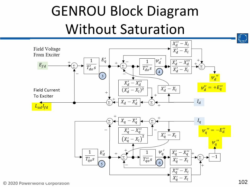
Summary of Equations as Block Diagram (Basically GENROU)
GENROU without Saturation

54© 2020 PowerWorld Corporation
Summary of What will be Modeled in Transient Stability
• Differential Equations will be modeled directly– The output of the differential equations will include
the internal voltage to apply to the network and the internal impedance
– 1 + ∆𝜔𝜔𝑝𝑝𝑝𝑝 𝐸𝐸𝑑𝑑′′ + 𝑗𝑗𝐸𝐸𝑞𝑞
′′
– 𝑅𝑅𝑠𝑠 + 𝑗𝑗𝑋𝑋𝑑𝑑′′
• Algebraic network equations are calculated across the entire system– Output of this will be new stator currents that are
inputs to the synchronous machine model – Output of new terminal voltages, currents, and power
will all feedback to other dynamic models (exciter, governor, etc) as well

55© 2020 PowerWorld Corporation
Reminder!
• Be careful looking at other textbooks and academic papers
• We have made arbitrary choices!– Our choice of defining of the rotor angle as the angle
between the a-axis and the q-axis effected all this math
– The definition of q-axis leading or lagging the d-axis effected all this math too
• I’ve wasted many days in the past decade getting confused when reading books and papers!– Books and Papers may have various 90 degree phase
shifts and sign differences– All comes down to these arbitrary choices

56© 2020 PowerWorld Corporation
Pause for a Moment
• We just got to a point where all this math has cleverly removed all the 𝜔𝜔𝑑𝑑 terms from everything!
• We have also converted the translation between the network equations and the rotating generator into a simple complex number rotation
• That was a very large amount of math• The choice of these reference frame
transformations matrices took engineers decades to figure out!
• Pause to thank the engineers from 50 - 80 years ago for working through all this

57© 2020 PowerWorld Corporation
Presentation so far applies to all Synchronous Machine Models
• However, – Magnetic Saturation hasn’t been introduced yet– Simplification due to machine construction for Salient Pole
Machines has been ignored• All synchronous machine models build from this point
– GENROU/GENROE (most directly, but with additive saturation)
– GENSAL/GENSAE (some older treatment of saturation, simplify Q axis)
– GENTPF (some simplification to dynamic model plus multiplicative saturation)
– GENTPJ (same as GENTPF but stator current also effects saturation)
– Prospective new models: GENQEC

58© 2020 PowerWorld Corporation
Nonlinear Magnetic Circuits
• Nonlinear magnetic models are needed because magnetic materials will saturate– Saturation means increasingly large amounts
of current are needed to increase the flux density
dtdN
dtdv
Rφλ
==
= 0
When linear λ = Li

59© 2020 PowerWorld Corporation
Saturation

60© 2020 PowerWorld Corporation
Relative Magnetic Strength Levels
• Earth’s magnetic field is between 30 and 70 mT (0.3 to 0.7 gauss)
• A refrigerator magnet might have 0.005 T• A commercial neodymium magnet might be 1 T• A magnetic resonance imaging (MRI) machine
would be between 1 and 3 T• Strong lab magnets can be 10 T• Frogs can be levitated at 16 T (see
www.ru.nl/hfml/research/levitation/diamagnetic• A neutron star can have 1 to 100 MT!

61© 2020 PowerWorld Corporation
Magnetic Saturation and Hysteresis
• The below image shows the saturation curves for various materials
Image Source: en.wikipedia.org/wiki/Saturation_(magnetic)
Magnetization curves of 9 ferromagnetic materials, showing saturation. 1.Sheet steel, 2.Silicon steel, 3.Cast steel, 4.Tungsten steel, 5.Magnet steel, 6.Cast iron, 7.Nickel, 8.Cobalt, 9.Magnetite; highest saturation materials can get to around 2.2 or 2.3T
H is proportional to current

62© 2020 PowerWorld Corporation
Magnetic Saturation and Hysteresis
• Magnetic materials also exhibit hysteresis, so there is some residual magnetism when the current goes to zero; design goal is to reduce the area enclosed by the hysteresis loop
Image source: www.nde-ed.org/EducationResources/CommunityCollege/MagParticle/Graphics/BHCurve.gif
To minimize the amountof magnetic material,and hence cost andweight, electric machinesare designed to operateclose to saturation

63© 2020 PowerWorld Corporation
Typical Saturation Tests PlotTerminal Voltage vs. Efd
• For those doing generator testing they will do tests to build the figure on left, but I like to flip axes and think about the figure on the right instead
Ifd
Vterm
Vterm
If at synchronous speed, then Terminal Voltage has same magnitude as stator flux
Ifd
64© 2020 PowerWorld Corporation
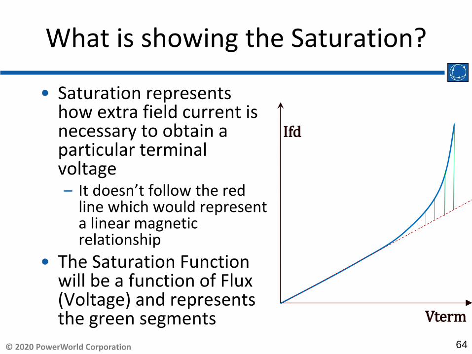
What is showing the Saturation?
• Saturation represents how extra field current is necessary to obtain a particular terminal voltage– It doesn’t follow the red
line which would represent a linear magnetic relationship
• The Saturation Function will be a function of Flux (Voltage) and represents the green segments
Ifd
Vterm

65© 2020 PowerWorld Corporation
Saturation is the “Extra” above what linear term represents
• Saturation Function is determined from generator testing by getting the purple line at the right
• Any function that approximates the purple shape can be used
• Different software tools and particular models use different functions
Efd
Vterm

66© 2020 PowerWorld Corporation
Description of Saturation in Software
• Two points on the saturation curve are provided as input data
• The saturation function is given. Can be different types– Quadratic– Scaled Quadratic– Exponential
1.0 1.2
S10
S12

67© 2020 PowerWorld Corporation
Saturation Function TypesName Function Which PlatformQuadratic 𝑆𝑆𝑆𝑆𝑑𝑑 𝑥𝑥 = 𝐵𝐵 𝑥𝑥 − 𝐴𝐴 2 GE PSLF
PowerWorld Simulator option
Scaled Quadratic 𝑆𝑆𝑆𝑆𝑑𝑑 𝑥𝑥 =
𝐵𝐵 𝑥𝑥 − 𝐴𝐴 2
𝑥𝑥PTI PSS/E, PowerWorld Simulator Option
Exponential 𝑆𝑆𝑆𝑆𝑑𝑑 𝑥𝑥 = 𝐵𝐵𝑥𝑥𝐴𝐴 BPA IPFSpecific models in PTI PSS/E Specific models in PowerWorld Simulator
68© 2020 PowerWorld Corporation
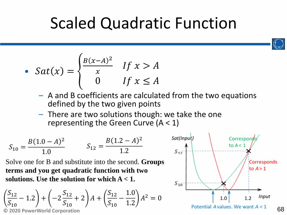
Scaled Quadratic Function
• 𝑆𝑆𝑆𝑆𝑑𝑑 𝑥𝑥 = �𝐵𝐵 𝑥𝑥−𝐴𝐴 2
𝑥𝑥𝐼𝐼𝐼𝐼 𝑥𝑥 > 𝐴𝐴
𝜋 𝐼𝐼𝐼𝐼 𝑥𝑥 ≤ 𝐴𝐴– A and B coefficients are calculated from the two equations
defined by the two given points– There are two solutions though: we take the one
representing the Green Curve (A < 1)
𝑆𝑆10 =𝐵𝐵 1.𝜋 − 𝐴𝐴 2
1.𝜋𝑆𝑆12 =
𝐵𝐵 1.2 − 𝐴𝐴 2
1.2
𝑆𝑆12
𝑆𝑆10− 1.2 + −2
𝑆𝑆12
𝑆𝑆10+ 2 𝐴𝐴 +
𝑆𝑆12
𝑆𝑆10−
1.𝜋1.2
𝐴𝐴2 = 𝜋
Solve one for B and substitute into the second. Groups terms and you get quadratic function with two solutions. Use the solution for which A < 1.

69© 2020 PowerWorld Corporation
Quadratic Function
• 𝑆𝑆𝑆𝑆𝑑𝑑 𝑥𝑥 = �𝐵𝐵 𝑥𝑥 − 𝐴𝐴 2 𝐼𝐼𝐼𝐼 𝑥𝑥 > 𝐴𝐴𝜋 𝐼𝐼𝐼𝐼 𝑥𝑥 ≤ 𝐴𝐴
– A and B coefficients are calculated from the two equations defined by the two given points
– There are two solutions though: we take the one representing the Green Curve (A < 1)
𝑆𝑆10 = 𝐵𝐵 1.𝜋 − 𝐴𝐴 2
𝑆𝑆12 = 𝐵𝐵 1.2 − 𝐴𝐴 2
𝑆𝑆12
𝑆𝑆10− 1.44 + −2
𝑆𝑆12
𝑆𝑆10+ 2.4 𝐴𝐴 +
𝑆𝑆12
𝑆𝑆10− 1.𝜋 𝐴𝐴2 = 𝜋
Solve one for B and substitute into the second. Groups terms and you get quadratic function with two solutions. Use the solution for which A < 1.

70© 2020 PowerWorld Corporation
Exponential Function
• 𝑆𝑆𝑆𝑆𝑑𝑑 𝑥𝑥 = 𝐵𝐵 𝑥𝑥 𝐴𝐴
– A and B coefficients are calculated from the two equations defined by the two given points
𝑆𝑆10 = 𝐵𝐵 1.𝜋 𝐴𝐴
𝑆𝑆12 = 𝐵𝐵 1.2 𝐴𝐴
𝑆𝑆10 = 𝐵𝐵
𝑆𝑆12 = S10 1.2 𝐴𝐴
𝑆𝑆12
𝑆𝑆10= 1.2 𝐴𝐴
ln𝑆𝑆12
𝑆𝑆10= ln 1.2 𝐴𝐴 = 𝐴𝐴 ln 1.2
𝐴𝐴 =ln 𝑆𝑆12
𝑆𝑆10ln 1.2
B = 𝑆𝑆10

71© 2020 PowerWorld Corporation
Implementing Saturation Models
• When implementing saturation models in code, it is important to recognize that the function is meant to be positive, so negative values are not allowed
• In large cases one is almost guaranteed to have special cases, sometimes caused by user typos– What to do if Se(1.2) < Se(1.0)?– What to do if Se(1.0) = 0 and Se(1.2) <> 0– What to do if Se(1.0) = Se(1.2) <> 0

72© 2020 PowerWorld Corporation
Where in Equations do you put Saturation: GENROU Example
GENROU with Saturation

73© 2020 PowerWorld Corporation
Where in Equations do you put Saturation: GENROU Example

74© 2020 PowerWorld Corporation
Saturation is being Added to the Sub-transient derivative
• Saturation is Added to the Field Current– This makes sense
especially because of the test that is used to find the saturation function
• The Open Circuit Saturation Test only finds saturation on D-Axis– We know there is also
saturation on Q-Axis– We simply assume it is the
proportional to the mutual inductance

75© 2020 PowerWorld Corporation
My Personal Assessment of GENROU saturation
• Why was it done this way?• This exactly matches the test which is done• A steady state open circuit test is done by varying
the field current and seeing what the terminal voltage of the synchronous machine does– This means 𝐼𝐼𝑑𝑑 = 𝐼𝐼𝑞𝑞 = 𝜋 (zero stator current)– In this open circuit test the q-axis fluxes are all zero!
(ψq) so we are only measuring the d-axis saturation• Varying the terminal voltage will vary the d-axis flux (ψd
′′)– If you have a curve showing you the extra field current
needed, in 1970 it made perfect sense to just add in that “extra” field current right into the block diagram
– This is exactly what GENROU represents

76© 2020 PowerWorld Corporation
Scaling of Saturation on q-Axis
• Mutual Inductance is something we skipped over earlier in our per unit parameterization choices (Page 30 – 42 of Sauer/Pai book)
• 𝑋𝑋𝑑𝑑 = 𝑋𝑋𝑚𝑚𝑑𝑑 + 𝑋𝑋𝑒𝑒 𝑋𝑋𝑚𝑚𝑑𝑑 = 𝑋𝑋𝑑𝑑 + 𝑋𝑋𝑒𝑒• 𝑋𝑋𝑞𝑞 = 𝑋𝑋𝑚𝑚𝑞𝑞 + 𝑋𝑋𝑒𝑒 𝑋𝑋𝑚𝑚𝑞𝑞 = 𝑋𝑋𝑞𝑞 + 𝑋𝑋𝑒𝑒
– 𝑋𝑋𝑑𝑑 and 𝑋𝑋𝑞𝑞 = synchronous reactance on d-axis and q-axis– 𝑋𝑋𝑚𝑚𝑑𝑑 and 𝑋𝑋𝑚𝑚𝑞𝑞: mutual inductance on the d-axis and q-axis
(this is the part inside the iron core so it saturates)– 𝑋𝑋𝑒𝑒 : the is the leakage inductance. This is the inductance
from the air gap, so we assume air does not saturate• The GENROU choice of scaling simply says the same
relative amount of saturation occurs on both d and q axis
• 𝑋𝑋𝑚𝑚𝑞𝑞
𝑋𝑋𝑚𝑚𝑑𝑑= 𝑋𝑋𝑞𝑞+𝑋𝑋𝑙𝑙
𝑋𝑋𝑑𝑑+𝑋𝑋𝑙𝑙: Scaling term to convert d-axis to q-axis

77© 2020 PowerWorld Corporation
Implications of modeling saturation with addition
• There were some fundamental relationships between the 4 rotor flux variables and how they relate to one another– By adding to ONLY two of those flux terms we have disrupted
those relationships• Saturation does NOT impact the network boundary equations
at all– As long as we require that 𝑋𝑋𝑑𝑑
′′ = 𝑋𝑋𝑞𝑞′′, a simple circuit equation can
be used at network boundary• 𝑋𝑋𝑑𝑑
′′ <> 𝑋𝑋𝑞𝑞′′ is called transient saliency and is not allowed in GENROU and
GENSAL models– This makes it much easier on software writers and is likely a big
reason why in 1970 this would have been picked as approximation
• Saturation is only a function of the flux and thus the terminal voltage of the synchronous machine– Saturation is NOT a function of armature current

78© 2020 PowerWorld Corporation
An Aside
• Beyond the scope of this presentation, but there are some fundamental theoretical flaws with the treatment of GENROU as well– Peter W. Sauer “Constraints on Saturation Modeling in
AC Machines”, IEEE Transactions on Energy Conversion, Vo. 7. No. 1, March 1992, pp. 161 – 167
– This paper discusses the fundamental assumption that the “coupling field” between the mechanical and electrical systems is a conservative (lossless) field
– That assumption puts some theoretical constraints on how the saturation should be applied to the equations
– A ton of calculus and algebra and you would get what I call the “GENPWS” (for Peter W. Sauer)

79© 2020 PowerWorld Corporation
An Aside“GENPWS” for Peter. W. Sauer
• Still uses addition– But the addition is made
to the input stator current instead
– Increasing stator current being fed into dynamic model increases the field voltage
– It’s a lot of math, but this makes some sense
– Does not change the fundamental relationships between all the rotor quantities

80© 2020 PowerWorld Corporation
Initialization of GENROU Model

81© 2020 PowerWorld Corporation
Initialization of GENROU with Saturation
• Write 5 equations as follows from Block Diagram at Steady State (inputs to integrators = 0)
• Know 𝑆𝑆𝑆𝑆𝑑𝑑 ψ′′ already (next slide)• Rotor Angle (δ) is in there too because we need it to perform
the translation from network to machine reference frame
1. 𝑋𝑋𝑑𝑑′ − 𝑋𝑋𝑒𝑒 𝐼𝐼𝑑𝑑 + ψ𝑑𝑑
′ − 𝐸𝐸𝑞𝑞′ = 𝜋 Sum inputs integrator for State 4
2. ψ𝑑𝑑′′ − 𝑋𝑋𝑑𝑑
′′−𝑋𝑋𝑙𝑙𝑋𝑋𝑑𝑑
′ −𝑋𝑋𝑙𝑙𝐸𝐸𝑞𝑞
′ − 𝑋𝑋𝑑𝑑′ −𝑋𝑋𝑑𝑑
′′
𝑋𝑋𝑑𝑑′ −𝑋𝑋𝑙𝑙
ψ𝑑𝑑′ = 𝜋 Final summation block resulting in ψ𝑑𝑑
′′
3. 𝑋𝑋𝑞𝑞 − 𝑋𝑋𝑞𝑞′ 𝐼𝐼𝑞𝑞 + ψ𝑞𝑞
′′ 𝑋𝑋𝑞𝑞−𝑋𝑋𝑙𝑙
𝑋𝑋𝑑𝑑−𝑋𝑋𝑙𝑙𝑆𝑆𝑆𝑆𝑑𝑑 ψ′′ − 𝐸𝐸𝑑𝑑
′ = 𝜋 Sum inputs integrator for State 6
4. 𝑋𝑋𝑞𝑞′ − 𝑋𝑋𝑒𝑒 𝐼𝐼𝑞𝑞 − ψ𝑞𝑞
′ + 𝐸𝐸𝑑𝑑′ = 𝜋 Sum inputs integrator for State 5
5. −ψ𝑞𝑞′′ − 𝑋𝑋𝑞𝑞
′′−𝑋𝑋𝑙𝑙
𝑋𝑋𝑞𝑞′ −𝑋𝑋𝑙𝑙
𝐸𝐸𝑑𝑑′ − 𝑋𝑋𝑞𝑞
′ −𝑋𝑋𝑞𝑞′′
𝑋𝑋𝑞𝑞′ −𝑋𝑋𝑙𝑙
ψ𝑞𝑞′ = 𝜋 Final summation block resulting in ψ𝑞𝑞
′′

82© 2020 PowerWorld Corporation
Getting Saturation Function at Initialization
• We can get the internal voltage on the network reference frame directly
• 𝑉𝑉𝑑𝑑 + 𝑉𝑉𝑑𝑑 = 𝑉𝑉𝑑𝑑𝑑𝑑𝑒𝑒𝑑𝑑𝑚𝑚 + 𝑗𝑗𝑉𝑉𝑑𝑑𝑑𝑑𝑒𝑒𝑑𝑑𝑚𝑚 + 𝑅𝑅𝑎𝑎 + 𝑗𝑗𝑋𝑋𝑑𝑑′′ 𝐼𝐼𝑑𝑑 + 𝑗𝑗𝐼𝐼𝑑𝑑
• 𝑉𝑉𝑑𝑑 = 𝑉𝑉𝑑𝑑𝑑𝑑𝑒𝑒𝑑𝑑𝑚𝑚 + 𝑅𝑅𝑎𝑎𝐼𝐼𝑑𝑑 − 𝑋𝑋𝑑𝑑′′𝐼𝐼𝑑𝑑
• 𝑉𝑉𝑑𝑑 = 𝑉𝑉𝑑𝑑𝑑𝑑𝑒𝑒𝑑𝑑𝑚𝑚 + 𝑅𝑅𝑎𝑎𝐼𝐼𝑑𝑑 + 𝑋𝑋𝑑𝑑′′𝐼𝐼𝑑𝑑
• From this we get the saturation function because the reference frame conversion only rotates, therefore the magnitude does not change!
• 𝑆𝑆𝑆𝑆𝑑𝑑 ψ′′ = 𝑆𝑆𝑆𝑆𝑑𝑑 𝑉𝑉𝑑𝑑 + 𝑗𝑗𝑉𝑉𝑑𝑑
• From here it’s a bit of clever algebra, but you can get the initial rotor angle
𝑆𝑆𝑆𝑆𝑑𝑑 ψ′′ = 𝑆𝑆𝑆𝑆𝑑𝑑 ψ𝑑𝑑′′ + 𝑗𝑗ψ𝑞𝑞
′′ = 𝑆𝑆𝑆𝑆𝑑𝑑 𝑉𝑉𝑞𝑞 − 𝑗𝑗𝑉𝑉𝑑𝑑 = 𝑆𝑆𝑆𝑆𝑑𝑑 𝑉𝑉𝑑𝑑 + 𝑗𝑗𝑉𝑉𝑞𝑞 𝑒𝑒𝑗𝑗 𝑑𝑑−𝜋𝜋2 = 𝑆𝑆𝑆𝑆𝑑𝑑 𝑉𝑉𝑑𝑑 + 𝑗𝑗𝑉𝑉𝑑𝑑

83© 2020 PowerWorld Corporation
Derivation of initial Rotor Angle for GENROU with Saturation

84© 2020 PowerWorld Corporation
Derivation of Initial Rotor Angle Continued

85© 2020 PowerWorld Corporation
GENROU without Saturation is Easier
• Rotor Angle can be obtained from network reference frame quantities
• If 𝐾𝐾𝑠𝑠𝑎𝑎𝑑𝑑 = 1.𝜋, that means there is no saturation– The rotor angle then simplifies to
– Sauer/Pai book page 51 will show finding the angle of the internal voltage using the following circuit
– Note: It’s kind of weird because thatis NOT the network interface as it uses 𝑋𝑋𝑞𝑞 instead of 𝑋𝑋𝑞𝑞
′′ +_𝑉𝑉𝑑𝑑 + 𝑗𝑗𝑉𝑉𝑑𝑑 𝑉𝑉𝑑𝑑𝑑𝑑𝑒𝑒𝑑𝑑𝑚𝑚 + 𝑗𝑗𝑉𝑉𝑑𝑑𝑑𝑑𝑒𝑒𝑑𝑑𝑚𝑚
𝐼𝐼𝑑𝑑 + 𝑗𝑗𝐼𝐼𝑑𝑑
+
_
𝑅𝑅𝑎𝑎 + 𝑗𝑗𝑋𝑋𝑞𝑞

86© 2020 PowerWorld Corporation
Initialization of the Remainder
• Rotor Angle known, continue with algebra• 𝑉𝑉𝑑𝑑 = 𝑉𝑉𝑑𝑑 sin δ − 𝑉𝑉𝑑𝑑 cos δ convert to dq axis using guess for δ
• 𝑉𝑉𝑞𝑞 = 𝑉𝑉𝑑𝑑 cos δ + 𝑉𝑉𝑑𝑑 sin δ convert to dq axis using guess for δ
• 𝐼𝐼𝑑𝑑 = 𝐼𝐼𝑑𝑑 sin δ − 𝐼𝐼𝑑𝑑 cos δ convert to dq axis using guess for δ
• 𝐼𝐼𝑞𝑞 = 𝐼𝐼𝑑𝑑 cos δ + 𝐼𝐼𝑑𝑑 sin δ convert to dq axis using guess for δ
• ψ𝑞𝑞′′ = − 𝑉𝑉
𝑑𝑑1+ω really we can ignore ω as it’s zero
• ψ𝑑𝑑′′ = + 𝑉𝑉
𝑞𝑞1+ω really we can ignore ω as it’s zero
• ψ𝑑𝑑′ = ψ𝑑𝑑
′′ − 𝐼𝐼𝑑𝑑 𝑋𝑋𝑑𝑑′′ − 𝑋𝑋𝑒𝑒 State 4. Algebra from summation blocks for ψ𝑑𝑑
′′
• 𝐸𝐸𝑞𝑞′ = ψ𝑑𝑑
′ + 𝐼𝐼𝑑𝑑 𝑋𝑋𝑑𝑑′ − 𝑋𝑋𝑒𝑒 State 3. Enforce zero input to state 4 integral block
• 𝐸𝐸𝑑𝑑′ = 𝐼𝐼𝑞𝑞 𝑋𝑋𝑞𝑞 − 𝑋𝑋𝑞𝑞
′ State 6. Enforce zero input to state 6 integral block
• ψ𝑞𝑞′ = 𝐸𝐸𝑑𝑑
′ + 𝐼𝐼𝑞𝑞 𝑋𝑋𝑞𝑞′ − 𝑋𝑋𝑒𝑒 State 5. Enforce zero input to state 5 integral block

87© 2020 PowerWorld Corporation
Machine Model Reactance Validation
• For synchronous machine models, there are d-axis and q-axis reactance values– Synchronous reactance : 𝑋𝑋𝑑𝑑 and 𝑋𝑋𝑞𝑞– Transient reactance : 𝑋𝑋𝑑𝑑
′ and 𝑋𝑋𝑞𝑞′
– Sub-transient reactance : 𝑋𝑋𝑑𝑑′′ and 𝑋𝑋𝑞𝑞
′′
– Leakage reactance : 𝑋𝑋𝑒𝑒• The following two relationships must be
satisfied (physically impossible to violate)– 𝑋𝑋𝑒𝑒 ≤ 𝑋𝑋𝑞𝑞
′′ ≤ 𝑋𝑋𝑞𝑞′ ≤ 𝑋𝑋𝑞𝑞
– 𝑋𝑋𝑒𝑒 ≤ 𝑋𝑋𝑑𝑑′′ ≤ 𝑋𝑋𝑑𝑑
′ ≤ 𝑋𝑋𝑑𝑑– These types of model errors are not uncommon

88© 2020 PowerWorld Corporation
Machine Reactance Auto-Correction in PowerWorld
• When machine reactance model errors are found and auto-correction is applied, the following changes will be applied to the data– If Xq’>Xq then Xq’=0.8Xq– If Xd’>Xd then Xd’=0.8Xd– If Xq”>Xq’ then Xq”=0.8Xq’– If Xd”>Xd’ then Xd”=0.8Xd’– If Xl >Xq” then Xl =0.8Xq”– If Xl >Xd” then Xl =0.8Xd”

89© 2020 PowerWorld Corporation
GENTPF/GENTPJ
• GENTPF Modifies the treatment of Saturation– Instead of being introduced as addition, consider treating
the input parameters as the “unsaturated parameters”• (Xd, Xq, Xdp, Xqp, Xdpp, Xqpp, Tdop, Tdopp,Tqop, Tqopp)• Then apply multiplication to account for saturation
– This has advantage of applying saturation to all the equations simultaneously
– GENTPJ also introduces the impact of the stator current on saturation.
• Empirical testings show that increases in stator current increases saturation.
– Again, we skipped all this, but the various parameters we derived
• GENTPF/GENTPJ however, does make a small change to the dynamic equations that may not have been quite right. We’re working on testing new models
90© 2020 PowerWorld Corporation
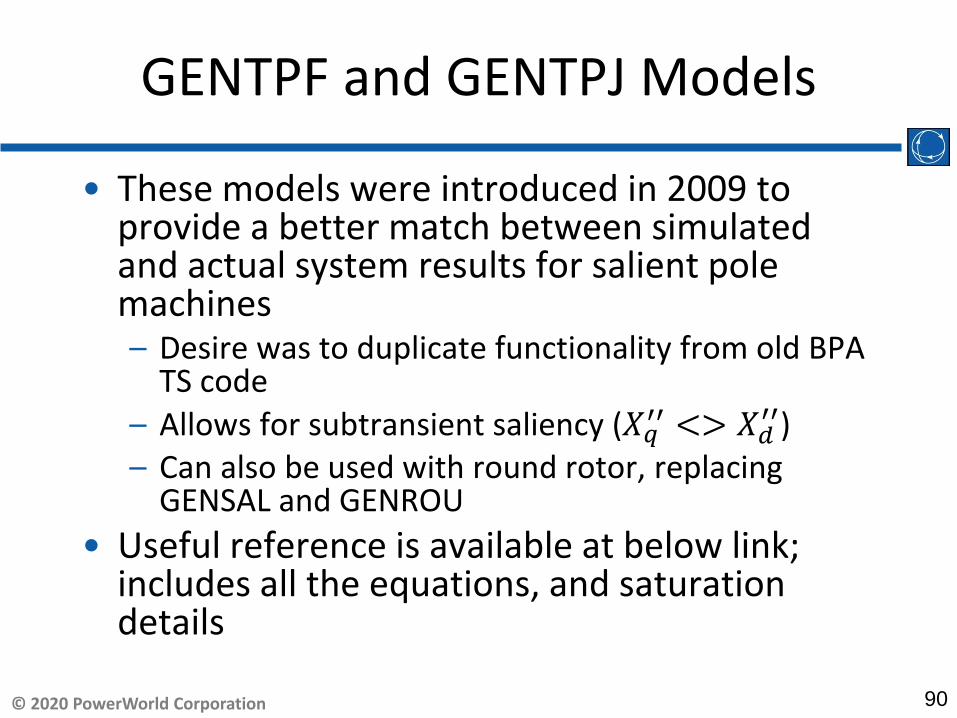
GENTPF and GENTPJ Models
• These models were introduced in 2009 to provide a better match between simulated and actual system results for salient pole machines– Desire was to duplicate functionality from old BPA
TS code– Allows for subtransient saliency (𝑋𝑋𝑞𝑞
′′ <> 𝑋𝑋𝑑𝑑′′)
– Can also be used with round rotor, replacing GENSAL and GENROU
• Useful reference is available at below link; includes all the equations, and saturation details

91© 2020 PowerWorld Corporation
Motivation for the Change: GENSAL Actual Results
Image source :https://www.wecc.biz/library/WECC%20Documents/Documents%20for%20Generators/Generator%20Testing%20Program/gentpj%20and%20gensal%20morel.pdf
Chief Josephdisturbance playbackGENSALBLUE = MODELRED = ACTUAL(Chief Joseph is a 2620 MW hydro plant on the Columbia River in Washington)

92© 2020 PowerWorld Corporation
GENTPJ Results
Chief Josephdisturbance playbackGENTPJBLUE = MODELRED = ACTUAL

93© 2020 PowerWorld Corporation
GENTPF and GENTPJ Models
Most of WECC machine models are now GENTPF or GENTPJ
If nonzero, Kis typically ranges from 0.02 to 0.12

94© 2020 PowerWorld Corporation
Network Equation for GENTPF/GENTPJ
• Network Equations can NOT use circuit equation• Results in some complexity we don’t discuss here
Electrical Torqueψ𝑞𝑞 = ψ𝑞𝑞
′′ − 𝐼𝐼𝑞𝑞𝑋𝑋𝑞𝑞𝑠𝑠𝑎𝑎𝑑𝑑′′ = −𝐸𝐸𝑑𝑑
′′ − 𝐼𝐼𝑞𝑞𝑋𝑋𝑞𝑞𝑠𝑠𝑎𝑎𝑑𝑑′′
ψ𝑑𝑑 = ψ𝑑𝑑′′ − 𝐼𝐼𝑑𝑑𝑋𝑋𝑑𝑑𝑠𝑠𝑎𝑎𝑑𝑑
′′ = +𝐸𝐸𝑞𝑞′′ − 𝐼𝐼𝑑𝑑𝑋𝑋𝑑𝑑𝑠𝑠𝑎𝑎𝑑𝑑
′′
𝑇𝑇𝑒𝑒𝑒𝑒𝑒𝑒𝑐𝑐 = ψ𝑑𝑑𝐼𝐼𝑞𝑞 − ψ𝑞𝑞𝐼𝐼𝑑𝑑
Saturated Subtransient Reactances
𝑋𝑋𝑑𝑑𝑠𝑠𝑎𝑎𝑑𝑑′′ = 𝑋𝑋𝑑𝑑
′′−𝑋𝑋𝑙𝑙𝑆𝑆𝑎𝑎𝑑𝑑𝑑𝑑
+ 𝑋𝑋𝑒𝑒
𝑋𝑋𝑞𝑞𝑠𝑠𝑎𝑎𝑑𝑑′′ = 𝑋𝑋𝑞𝑞
′′−𝑋𝑋𝑙𝑙
𝑆𝑆𝑎𝑎𝑑𝑑𝑞𝑞+ 𝑋𝑋𝑒𝑒
Network Interface Equations𝑉𝑉𝑑𝑑 + 𝑗𝑗𝑉𝑉𝑞𝑞 = 𝐸𝐸𝑑𝑑
′′ + 𝑗𝑗𝐸𝐸𝑞𝑞′′ 1 + 𝜔𝜔
Because 𝑋𝑋𝑞𝑞𝑠𝑠𝑎𝑎𝑑𝑑′′ <> 𝑋𝑋𝑑𝑑𝑠𝑠𝑎𝑎𝑑𝑑
′′ we cannot use a circuit model for network interface equations and must instead directly use the following.
𝑉𝑉𝑑𝑑𝑑𝑑𝑒𝑒𝑑𝑑𝑚𝑚 = 𝑉𝑉𝑑𝑑 − 𝑅𝑅𝑎𝑎𝐼𝐼𝑑𝑑 + 𝑋𝑋𝑞𝑞𝑠𝑠𝑎𝑎𝑑𝑑′′ 𝐼𝐼𝑞𝑞
𝑉𝑉𝑞𝑞𝑑𝑑𝑒𝑒𝑑𝑑𝑚𝑚 = 𝑉𝑉𝑞𝑞 − 𝑋𝑋𝑑𝑑𝑠𝑠𝑎𝑎𝑑𝑑′′ 𝐼𝐼𝑑𝑑 − 𝑅𝑅𝑎𝑎𝐼𝐼𝑞𝑞

95© 2020 PowerWorld Corporation
Theoretical Justification for GENTPF and GENTPJ
• In the GENROU and GENSAL models saturation shows up purely as an additive term of Eq’ and Ed’– Saturation does not come into play in the network
interface equations and thus with the assumption of 𝑋𝑋𝑞𝑞𝑠𝑠𝑎𝑎𝑑𝑑
′′ = 𝑋𝑋𝑑𝑑𝑠𝑠𝑎𝑎𝑑𝑑′′ a simple circuit model can be used
• The advantage of the GENTPF/J models is saturation really affects the entire model, and in this model it is applied to all the inductance terms simultaneously– This complicates the network boundary equations, but
since these models are designed for 𝑋𝑋𝑞𝑞𝑠𝑠𝑎𝑎𝑑𝑑
′′ <> 𝑋𝑋𝑑𝑑𝑠𝑠𝑎𝑎𝑑𝑑′′ there is no increase in complexity

96© 2020 PowerWorld Corporation
GENTPF/GENTPJ: However?
• If you look at the differential equations, they are different!– In particular notice that the leakage reactance is NOT
on the block diagram for the differential equations– The GENTPF/GENTPJ differential equations represent
what would happen to the GENROU equations if you make the approximation on each axis
• 𝑋𝑋𝑒𝑒 = 𝑋𝑋𝑑𝑑′′ on the d-axis differential equations
• 𝑋𝑋𝑒𝑒 = 𝑋𝑋𝑞𝑞′′ on the q-axis differential equations
• This has some undesired effects on the transient response– Quincy Wang at PowerTech (now at B.C. Hydro) first
pointed this out to me a few years ago

97© 2020 PowerWorld Corporation
Why does this even matter?
• GENROU and GENSAL models date from 1970, and their purpose was to replicate the dynamic response the synchronous machine– They have done a great job doing that
• Weaknesses of the GENROU and GENSAL model has been found to be with matching the field current and field voltage measurements– Field Voltage/Current may have been off a little bit,
but that didn’t effect dynamic response– It just shifted the values and gave them an offset
• Shifted/Offset field voltage/current didn’t matter too much in the past

98© 2020 PowerWorld Corporation
Over and Under Excitation Limiters
• Traditionally our industry has not modeled over excitation limiters (OEL) and under excitation limiters (UEL) in transient stability simulation– The Mvar outputs of synchronous machines during
transients likely do go outside these bounds in our existing simulations
– Our Simulation haven’t been modeling limits being hit anyway, so the overall dynamic response isn’t impacted
• If the industry wants to start modeling OEL and UEL, then we need to better match the field voltage and currents– Otherwise we’re going to be hitting these limits when
in real life we are not

99© 2020 PowerWorld Corporation
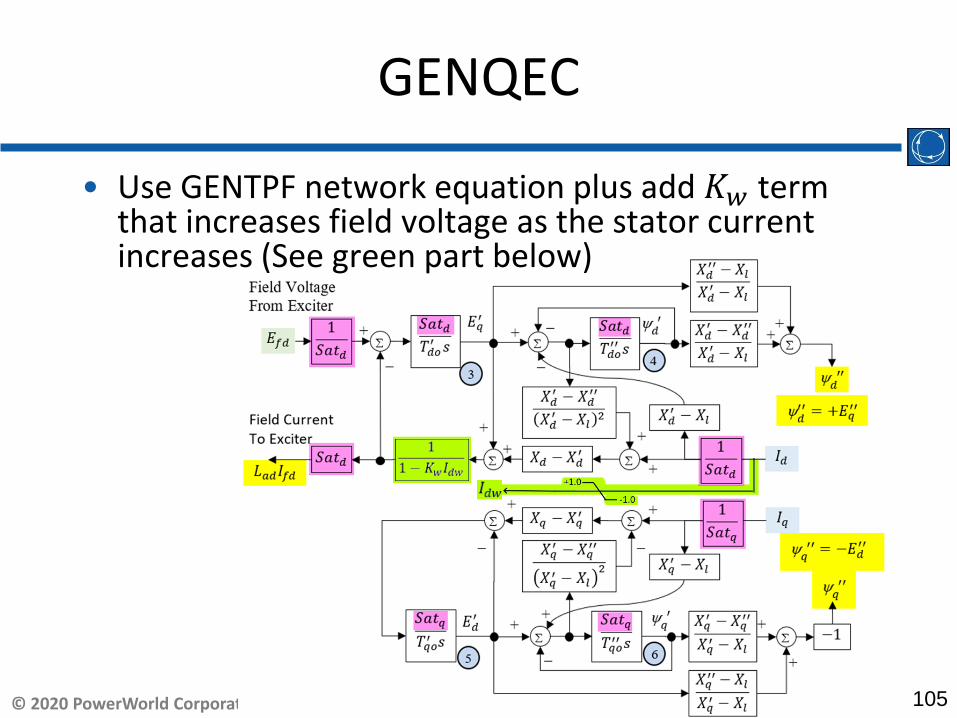
GENQEC
• Saurav Mohapatra and Jamie Weber at PowerWorldCorporation have been working with Quincy Wang at BC Hydro on a “GENQEC”
• We agreed on two main points!– Saturation function should be applied to all input
parameters by multiplication • This also ensures a conservative coupling field assumption of
Peter W. Sauer paper from 1992– Same multiplication should be applied to both d-axis and q-
axis terms (assume same amount of saturation on both)• Results in differential equations that are nearly the
same as GENROU – Scales the inputs and outputs, and effects time constants
• Network Interface Equation is same as GENTPF/J

100© 2020 PowerWorld Corporation
Applying Saturation to the Dynamic Equations
• From machine design and analysis, these are the reactance values that saturate: Xmd, Xfd, X1d, and Xmq, X1q, X2q– Go back to Sauer/Pai book to see what these are
• Assume leakage reactance does NOT saturate: Xl
• In transient stability, we use transformed constants: Xd, Xd
′ , Xd′′, and Xq, Xq
′ , Xq′′
• GENTPF/GENTPJ used following in network boundary equations
Xdsat′′ =
Xd′′ − Xl
𝑆𝑆𝑆𝑆𝑑𝑑d+ Xl Xqsat
′′ =Xq
′′ − Xl
𝑆𝑆𝑆𝑆𝑑𝑑q+ Xl

101© 2020 PowerWorld Corporation
GENQEC – Extend concept used in GENTPJ algebraic network equations
d-axis q-axis
ReactanceValues
Xdsat′′ = Xd
′′−Xl𝑆𝑆𝑎𝑎𝑑𝑑d
+ Xl Xqsat′′ = Xq
′′−Xl𝑆𝑆𝑎𝑎𝑑𝑑q
+ Xl
Xdsat′ = Xd
′ −Xl𝑆𝑆𝑎𝑎𝑑𝑑d
+ Xl Xqsat′ = Xq
′ −Xl𝑆𝑆𝑎𝑎𝑑𝑑q
+ Xl
Xdsat = Xd−Xl𝑆𝑆𝑎𝑎𝑑𝑑d
+ Xl Xqsat = Xq−Xl𝑆𝑆𝑎𝑎𝑑𝑑q
+ Xl
Time Constants(are a function of reactance values)
Tdosat′ = Tdo
′
𝑆𝑆𝑎𝑎𝑑𝑑dTqosat
′ = Tqo′
𝑆𝑆𝑎𝑎𝑑𝑑q
Tdosat′′ = Tdo
′′
𝑆𝑆𝑎𝑎𝑑𝑑dTqosat
′′ = Tqo′′
𝑆𝑆𝑎𝑎𝑑𝑑q
Exciter Interface Signals
𝐸𝐸fdsat = 𝐸𝐸fd𝑆𝑆𝑎𝑎𝑑𝑑d
Xmdsat𝐼𝐼fd = Xdsat − Xl 𝐼𝐼fd = Xd−Xl𝑆𝑆𝑎𝑎𝑑𝑑d
𝐼𝐼fd
102© 2020 PowerWorld Corporation
GENROU Block Diagram Without Saturation

103© 2020 PowerWorld Corporation
GENQEC Basic Diagram

104© 2020 PowerWorld Corporation
GENQEC
• Quincy tests and other tests showed that the slope of the Vterm vs. Ifd curve changed as the generator is loaded.– This slope changes occurred immediately– This is what we are calling “compensation”
Ifd
Vterm
Open CircuitTest
Load TestWith Id < 𝜋 Load Test
With Id > 𝜋
105© 2020 PowerWorld Corporation
GENQEC
• Use GENTPF network equation plus add 𝐾𝐾𝑛𝑛 term that increases field voltage as the stator current increases (See green part below)

106© 2020 PowerWorld Corporation
Comment about all these Synchronous Machine Models
• We are improving these models– Does not mean the old models were useless
• All these models have the same input parameter names, but that does not mean they are exactly the same– Input parameters are tuned for a particular model– It is NOT appropriate to take the all the
parameters for GENROU and just copy them over to a GENTPJ model and call that your new model
– When performing a new generator testing study, that is the time to update the parameters

107© 2020 PowerWorld Corporation
Status of these models
• Applying saturation using multiplication is definitely better theoretically– Maintains the relationships between the rotor fluxes as
they all scale the same• Multiplication saturation has shown better
experimental results – GENTPF/GENTPJ results are related to this– Quincy at BC Hydro has confirmed good fits with GENQEC– Saurav at PowerWorld confirmed good fits to test data
using an earlier version of this model we called GENTPW• The GENQEC model’s Kw term is another
experimentally determined parameter to add to the model– It removes the need for the Kis parameter, as the addition
of the compensation factor gives a similar effect of stator current impacting the field current and voltage

108© 2020 PowerWorld Corporation
PowerWorld’s hope for GENQEC
• PowerWorld had hopes of figuring out some theoretical relationship from cross saturation (currents on the d-axis creating saturation on the q-axis and vice-versa) that would explain the need for Kw term and lead to both good experimental results and better theoretical justification
• Status: We give up!• GENQEC Kw term is explainable from the
experimental test data. • We leave it to another Ph.D. student someday to
help explain better why this is needed

109© 2020 PowerWorld Corporation
Input Parameters in Dialog
• Stability Tab• Machine
ModelTab
110© 2020 PowerWorld Corporation
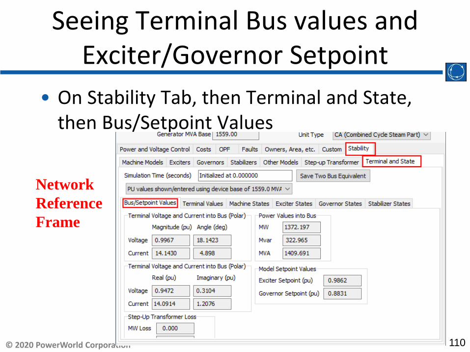
Seeing Terminal Bus values and Exciter/Governor Setpoint
• On Stability Tab, then Terminal and State, then Bus/Setpoint Values
NetworkReferenceFrame

111© 2020 PowerWorld Corporation
Seeing Terminal Values
• On Stability Tab, then Terminal and State, then Terminal Values
𝐼𝐼𝑞𝑞𝐼𝐼𝑑𝑑
𝑉𝑉𝑞𝑞𝑑𝑑𝑒𝑒𝑑𝑑𝑚𝑚𝑉𝑉𝑑𝑑𝑑𝑑𝑒𝑒𝑑𝑑𝑚𝑚
𝑉𝑉𝑑𝑑 𝑉𝑉𝑞𝑞
𝐸𝐸𝑓𝑓𝑑𝑑
𝐿𝐿𝑎𝑎𝑑𝑑𝐼𝐼𝑓𝑓𝑑𝑑
Machine Reference Frame
δ
112© 2020 PowerWorld Corporation
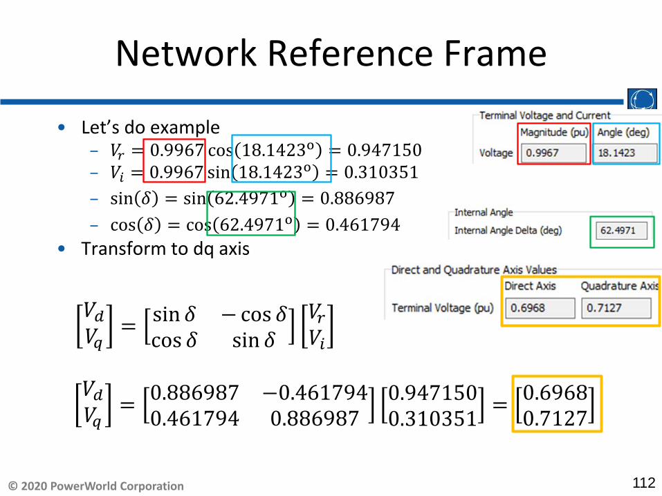
Network Reference Frame
• Let’s do example– 𝑉𝑉𝑑𝑑 = 𝜋.99𝜋7 cos 18.1423o = 𝜋.94715𝜋– 𝑉𝑉𝑑𝑑 = 𝜋.99𝜋7 sin 18.1423o = 𝜋.31𝜋351– sin 𝛿𝛿 = sin 𝜋2.4971o = 𝜋.88𝜋987– cos 𝛿𝛿 = cos 𝜋2.4971o = 𝜋.4𝜋1794
• Transform to dq axis
𝑉𝑉𝑑𝑑𝑉𝑉𝑞𝑞
= sin 𝛿𝛿 − cos 𝛿𝛿cos 𝛿𝛿 sin 𝛿𝛿
𝑉𝑉𝑑𝑑𝑉𝑉𝑑𝑑
𝑉𝑉𝑑𝑑𝑉𝑉𝑞𝑞
= 𝜋.88𝜋987 −𝜋.4𝜋1794𝜋.4𝜋1794 𝜋.88𝜋987
𝜋.94715𝜋𝜋.31𝜋351 = 𝜋.𝜋9𝜋8
𝜋.7127

113© 2020 PowerWorld Corporation
Seeing the Model States
• On Stability Tab, then Terminal and State, then Terminal Values
ψ𝑑𝑑′
ψ𝑞𝑞′′
𝐸𝐸𝑑𝑑′
𝐸𝐸𝑞𝑞′
ω
δ=1.0908 radians= 62.4971 degrees
δ

114© 2020 PowerWorld Corporation
Model Simplifications
• Newer models (GENTPF/GENTPJ, GENQEC) have particular input parameter combinations to indicate model simplifications
• Salient Pole Machine with a single amortisseurwinding
• Salient Pole Machine without any amortisseurwindings
• 𝑋𝑋𝑞𝑞 = 𝑋𝑋𝑞𝑞′
• 𝑇𝑇𝑞𝑞𝑑𝑑′ = 𝜋
• 𝑋𝑋𝑞𝑞 = 𝑋𝑋𝑞𝑞′
= 𝑋𝑋𝑞𝑞′′
• 𝑋𝑋𝑑𝑑′
= 𝑋𝑋𝑑𝑑′′
• 𝑇𝑇𝑞𝑞𝑑𝑑′ = 𝑇𝑇𝑑𝑑𝑑𝑑
′′ = 𝑇𝑇𝑞𝑞𝑑𝑑′′ = 𝜋
• 𝑇𝑇𝑑𝑑𝑑𝑑′ > 𝜋

115© 2020 PowerWorld Corporation
Simplification for GENQEC for Salient Pole with 1 amortisseur
• q-axis is simplified to
• This becomes
𝑋𝑋𝑞𝑞 = 𝑋𝑋𝑞𝑞′
and 𝑇𝑇𝑞𝑞𝑑𝑑′ = 𝜋,

116© 2020 PowerWorld Corporation
GENQEC simplified
• Salient Pole with 1 amortisseur
• 𝑋𝑋𝑞𝑞 = 𝑋𝑋𝑞𝑞′
• 𝑇𝑇𝑞𝑞𝑑𝑑′ = 𝜋

117© 2020 PowerWorld Corporation
Reminder: Xd and Xq have physical meaning: Example WECC
𝑿𝑿𝒒𝒒′ /𝑿𝑿𝒒𝒒
About 75% are Clearly Salient Pole Machines!

118© 2020 PowerWorld Corporation
Simplification for GENQEC for Salient Pole with no amortisseur
• 𝑋𝑋𝑞𝑞 = 𝑋𝑋𝑞𝑞′
= 𝑋𝑋𝑞𝑞′′
• 𝑋𝑋𝑑𝑑′
= 𝑋𝑋𝑑𝑑′′
• 𝑇𝑇𝑞𝑞𝑑𝑑′ = 𝑇𝑇𝑑𝑑𝑑𝑑
′′ = 𝑇𝑇𝑞𝑞𝑑𝑑′′ = 𝜋
• 𝑇𝑇𝑑𝑑𝑑𝑑′ > 𝜋

119© 2020 PowerWorld Corporation
Simplification for GENQEC for Salient Pole with 0 amortisseur
• This becomes the following. The yellow highlighted blocks are infinitely fast delay blocks which simplify to 3 algebraic equations
• 𝐸𝐸𝑑𝑑′ = 𝜋
• ψ𝑑𝑑′ = 𝐸𝐸𝑞𝑞
′ − 𝐼𝐼𝑑𝑑𝑋𝑋𝑑𝑑
′ −𝑋𝑋𝑙𝑙𝑆𝑆𝑎𝑎𝑑𝑑𝑑𝑑
• ψ𝑞𝑞′ = 𝐸𝐸𝑑𝑑
′ + 𝐼𝐼𝑞𝑞𝑋𝑋𝑞𝑞
′ −𝑋𝑋𝑙𝑙
𝑆𝑆𝑎𝑎𝑑𝑑𝑑𝑑

120© 2020 PowerWorld Corporation
GENQEC for no amortisseurwindings
• 𝑋𝑋𝑞𝑞 = 𝑋𝑋𝑞𝑞′
= 𝑋𝑋𝑞𝑞′′
• 𝑋𝑋𝑑𝑑′
= 𝑋𝑋𝑑𝑑′′
• 𝑇𝑇𝑞𝑞𝑑𝑑′ = 𝑇𝑇𝑑𝑑𝑑𝑑
′′ = 𝑇𝑇𝑞𝑞𝑑𝑑′′ = 𝜋
• 𝑇𝑇𝑑𝑑𝑑𝑑′ > 𝜋