synchronized swept-sine: theory, application, and
TRANSCRIPT
HAL Id: hal-02504321https://hal.archives-ouvertes.fr/hal-02504321
Submitted on 10 Mar 2020
HAL is a multi-disciplinary open accessarchive for the deposit and dissemination of sci-entific research documents, whether they are pub-lished or not. The documents may come fromteaching and research institutions in France orabroad, or from public or private research centers.
L’archive ouverte pluridisciplinaire HAL, estdestinée au dépôt et à la diffusion de documentsscientifiques de niveau recherche, publiés ou non,émanant des établissements d’enseignement et derecherche français ou étrangers, des laboratoirespublics ou privés.
Synchronized Swept-Sine: Theory, Application, andImplementation
Antonin Novak, Laurent Simon, Pierrick Lotton
To cite this version:Antonin Novak, Laurent Simon, Pierrick Lotton. Synchronized Swept-Sine: Theory, Application, andImplementation. Journal of the Audio Engineering Society, Audio Engineering Society, 2015, 63 (10),pp.786-798. �10.17743/jaes.2015.0071�. �hal-02504321�

Synchronized Swept-Sine:
Theory, Application and Implementation
Antonin Novak∗, Laurent Simon, Pierrick Lotton
Laboratoire d’Acoustique de l’Universite du Mans, LAUM - UMR 6613 CNRS, Le Mans Universite, Avenue Olivier
Messiaen, 72085 LE MANS CEDEX 9, France∗[email protected]∗https://ant-novak.com
Abstract
Exponential, or sometimes called logarithmic, swept-sine signal is very often used to analyze nonlinear audio systems. In
this paper, the theory of exponential swept-sine measurements of nonlinear systems is reexamined. The synchronization
procedure necessary for a proper analysis of higher harmonics is detailed leading to an improvement of the formula for
the exponential swept-sine signal generation. Moreover, an analytical expression of spectra of the swept-sine signal
is derived and used in the deconvolution of the impulse response. A Matlab code for generation of the synchronized
swept-sine, deconvolution, and separation of the impulse responses is given with discussion of some application issues
and an illustrative example of harmonic analysis of current distortion of a woofer is provided.
The archived file is not the final published version of the article A. Novak, P. Lotton & L. Simon (2015), ”Synchronized
Swept-Sine: Theory, Application, and Implementation”, Journal of the Audio Engineering Society. Vol. 63(10), pp.
786-798.
The definitive publisher-authenticated version is available online at https://doi.org/10.17743/jaes.2015.0071,
Readers must contact the publisher for reprint or permission to use the material in any form.
LA
UM
,C
NR
SU
MR
66
13
1

Novak et al. Synchronized Swept-Sine — 2/21
1. INTRODUCTION
A swept-sine, also called a chirp, is a widely used signal for characterizing a frequency response of a linear system
under test. A technique for analysis of nonlinear system (NLS) based on an exponential swept-sine signal has been
first presented by Farina in 2000. This technique enables a separation of impulse responses for each harmonic
distortion order [1]. Later, Farina called this technique the ”nonlinear convolution” [2]. It is worth noting that the
idea of separation of harmonic products when using the swept-sine signals was mentioned earlier in [3, 4].
Since 2000, the method has been used in many applications, namely in fields of audio and acoustics, e.g. for
Room Impulse Response (RIR) measurements [5, 6], for measurement of Head-Related Transfer Functions (HRTF)
and Head-Related Impulse Responses (HRIR) [7, 8], in nonlinear acoustics [9, 10], and in many other applications
in acoustics [11, 12, 13, 14].
The need to synchronize the exponential swept-sine signal for purpose of nonlinear system identification has
been first presented in [15] and the mathematical background for the identification of nonlinear systems using the
exponential swept-sine signal has been then given in [16]. The importance of the synchronization of the swept-sine
signal for identification of a cascade of Hammerstein systems has been also pointed out in [17]. It has also been
shown in [18] that the method based on the exponential swept-sine signal can be used to identify two nonlinear
systems in series.
In this paper, we reformulate the exponential swept-sine method. After a short review of the method presented in
Sec. 2 we derive the form of the exponential swept-sine signal suitable for the estimation of so-called Higher Harmonic
Frequency Responses (HHFRs) in Sec. 3. This form differs from the one usually used with the exponential swept-
sine methods and we focus on consequences of different definitions. Next, the analytical formula for the spectra of
the synchronized swept-sine signal is derived in Appendix and used for the deconvolution in Sec. 4. In Sec. 5, the
separation of higher harmonic impulse responses is described and the advantage of using the analytical formula in
deconvolution procedure is discussed. The most important equations for the synchronized swept-sine method are
then summarized in Sec. 6. Finally, we provide an illustrative example in Sec. 7 in which we analyze higher harmonics
of current distortion of a woofer using both the synchronized and the non-synchronized swept-sine signals and we
compare the results with a sine-based measurement. Moreover, in Sec. A.2 a Matlab code for all the important
steps of the method is provided and some implementation issues are discussed.
2. Brief Review Of the Swept-Sine Method
Regarding the basics of NLS theory, when a sine-wave is used as an input signal higher harmonics appear at the
output of the NLS as multiples of the input driving frequency. The amplitude and phase of all the higher harmonics
may be furthermore frequency dependent. In this section, we briefly recall the main steps of the exponential swept-
sine method to separate the frequency dependent higher harmonics by using a single swept-sine measurement.
The exponential swept-sine method can be summarized in the following steps:
• generation of the exponential swept-sine input signal
• acquisition of the response of the nonlinear system under test to the exponential swept-sine signal
• impulse response deconvolution
• separation of the higher harmonic impulse responses hn(t) and estimation of so-called Higher Harmonic
Frequency Responses (HHFRs) Hn(f) (Fourier transform of the higher harmonic impulse responses)
2.1 Exponential Swept-Sine Signal Generation
The exponential swept-sine signal can be generated either directly in the time domain or indirectly in the frequency
domain as discussed in [19]. The generation in time domain can be realized using a direct-implementation method,
LA
UM
,C
NR
SU
MR
66
13

Novak et al. Synchronized Swept-Sine — 3/21
also discussed in [19], or using a mathematical formula given by Farina in [1] as
x(t) = sin
{2πf1T
ln(f2/f1)
[exp
(t
Tln(
f2f1
)
)− 1
]}, (1)
where f1 is the initial frequency, f2 is the final frequency and T is the time duration of the swept-sine signal.
It has been shown in [16] that the swept-sine signal must be generated in a slightly different way in order to
be able to estimate both amplitude and phase of HHRFs properly. The modified signal is called synchronized
swept-sine. It is generated according to [16] as
x(t) = sin
{2πf1L
[exp
(t
L
)− 1
]}, (2)
L being the rate of frequency increase defined as
L =1
f1round
T f1
ln(f2f1
) , (3)
where T is an approximate time length of the signal x(t) and round represents rounding towards nearest integer.
According to [16], the rounding operation is necessary to avoid an incorrect phase estimation of HHRFs. The phase
synchronization of HHFRs has been successfully used in several works dealing with nonlinear system identification
in acoustics [8, 20].
2.2 Impulse Response Deconvolution
The exponential swept-sine signal x(t) is then used as the input to the nonlinear system under test and the output
y(t) signal is acquired. To obtain the impulse response h(t) of the nonlinear system under test, we deconvolve the
output signal y(t) with the original swept-sine signal x(t).
The deconvolution can be made either in time or in frequency domain. The classical approach consists in
deconvolution by division in frequency domain as
h(t) = F−1[F [y(t)]
F [x(t)]
], (4)
where x(t) is the swept-sine signal, y(t) is the (system) response to x(t) and F and F−1 are direct and inverse Fourier
transforms respectively. A regularization function should be added in order to avoid division by zero problems since
F [x(t)] approach zero below f1 and above f2 [19, 21].
The approach introduced by Farina [1] consists in using a so-called inverse filter x(t) defined in such a way that,
when convolved with the swept-sine signal x(t), we get the Dirac delta function δ(t)
x(t) ∗ x(t) = δ(t). (5)
According to [21], the inverse filter is a time-reversal of the swept-sine signal x(t) with +3 dB/octave slope. The
deconvolution can then be realized either in the time domain
h(t) = y(t) ∗ x(t), (6)
or in frequency domain
h(t) = F−1 [F [y(t)]F [x(t)]] . (7)
LA
UM
,C
NR
SU
MR
66
13

Novak et al. Synchronized Swept-Sine — 4/21
2.3 Higher Harmonic Impulse Responses Separation
The deconvolution process results in the impulse response h(t) which is a summation of time-shifted higher harmonic
impulse responses hn(t) [1, 16]. They can be easily separated by windowing in the time domain as described in
[1, 19]. Finally, they can be Fourier transformed to calculate the HHFRs as
Hn(f) = F [hn(t)] . (8)
The magnitude plot of Hn(f) in dB is the most common representation since it shows the amount of distortion of
all the harmonics as a function of frequency [1].
3. Synchronized Swept-Sine Signal Generation
In this section we focus on the generation of the exponential swept-sine signal. We give the mathematical background
to the choice of the form of the signal and we explain why the synchronization of the swept-sine signal is necessary
for a correct estimation of the HHFRs Hn(f).
3.1 Conditioning the Swept-Sine Signal
The properties of the exponential swept-sine signal generated either using (1) or (2) have been studied in [1] and
[16] respectively. Instead of discussing the properties of a given exponential swept-sine signal, we can formulate
the problem in another way and rise the following question: What kind of swept-sine signal can be used for the
estimation of the HHFRs Hn(f)?
To answer this question, we start with a general definition of a swept-sine signal x(t) with an unknown phase
ϕ(t)
x(t) = sin [ϕ(t)] , (9)
and we consider the response y(t) of the NLS to such a signal as a sum of higher harmonics as
y(t) =
∞∑n=1
sin [nϕ(t)] ∗ hn(t). (10)
Considering that the response y(t) of the NLS to the swept-sine signal x(t) is simply a convolution of the latter
with an impulse response h(t)
y(t) = x(t) ∗ h(t), (11)
we want the impulse response to be a sum of the time-delayed higher harmonic impulse responses hn(t) as
h(t) =
∞∑n=1
hn(t+ ∆tn), (12)
so that they can be easily separated from each other. From (9), (11), and (12) we can write
y(t) = sin [ϕ(t)] ∗∞∑n=1
hn(t+ ∆tn). (13)
Comparing the output y(t) from (10) and (13) we get
∞∑n=1
sin [nϕ(t)] ∗ hn(t) = sin [ϕ(t)] ∗∞∑n=1
hn(t+ ∆tn), (14)
and putting the input signal sin [ϕ(t)] inside the convolution sum, we can write
∞∑n=1
sin [nϕ(t)] ∗ hn(t) =
∞∑n=1
sin [ϕ(t)] ∗ hn(t+ ∆tn). (15)
LA
UM
,C
NR
SU
MR
66
13
Novak et al. Synchronized Swept-Sine — 5/21
Both sums of Eq. (15) are equal if the convolution terms inside the sum are equal as well. Expressing the inside
convolution equality leads to ∫ ∞−∞
sin [nϕ(u)]hn(t− u)du =∫ ∞−∞
sin [ϕ(v)]hn(t+ ∆tn − v)dv. (16)
Substituting v = τ + ∆tn, we get∫ ∞−∞
sin [nϕ(u)]hn(t− u)du =∫ ∞−∞
sin [ϕ(τ + ∆tn)]hn(t− τ)dτ, (17)
which can be solved by imposing
sin [nϕ(t)] = sin [ϕ(t+ ∆tn)] . (18)
In other words, the signal we are looking for must have the following property: shifting the signal in time by
∆tn is equivalent to generating the same signal with n-times higher phase.
3.2 Synchronizing the Swept-Sine Signal
The condition given in (18) can be solved using
nϕ(t) = ϕ(t+ ∆tn) + 2πl, ∀l ∈ Z. (19)
This equation has a form similar to that of a Delayed Differential Equation [22], which may have an oscillatory
solution leading to a phase / frequency modulated signal, or to an exponential solution leading to a swept-sine
signal. Focusing on the exponential solution, we consider a trial solution in form of an exponential function as
ϕ(t) = A exp (αt) , (20)
and inserting the trial solution back to (19), we find that
∆tn =ln(n− 2πl
A exp(αt) )
α. (21)
Since we want ∆tn to be independent on time t, we must impose l = 0 and we then get
α =ln(n)
∆tn. (22)
To summarize this part, we prove that the signal x(t) has a form of
x(t) = sin [A exp (αt)] , (23)
where the coefficient A acts as a rate of sweeping change and where the coefficient α is still unknown. To find
the relation between these two coefficients and the parameters of the swept-sine, such as the initial and the final
frequencies f1 and f2 and the time duration T , the following steps must be completed.
LA
UM
,C
NR
SU
MR
66
13

Novak et al. Synchronized Swept-Sine — 6/21
3.3 Initial and Final Frequencies
First, we define the instantaneous frequency of the signal x(t) from (20) as
fi(t) =1
2π
dϕ(t)
dt=Aα
2πexp (αt) . (24)
At initial time t = 0, the initial frequency is denoted fi(0) = f1, leading to
α =2πf1A
. (25)
At final time t = T , the final frequency is denoted fi(T ) = f2, leading to
f1 exp
(2πf1A
T
)= f2, (26)
and thus
A =2πf1T
ln(f2f1
) . (27)
So, the formula for the synchronized swept-sine signal can be written as
x(t) = sin
[2πf1T
ln(f2/f1)exp
(t
Tln(
f2f1
)
)]. (28)
Note that this formula is almost equivalent to the one given in (1) except for the ”−1” term at the end of (1) that
is missing in (28).
3.4 Initial Phase
When examining the missing term ”−1” in (28) in comparison with (1), we first note, that the term ”−1” in (1)
ensures having the initial phase to be zero, which is not the case in (28), where the initial phase is given by the
term
ϕ(0) =2πf1T
ln(f2/f1). (29)
However, fixing the phase to be zero by adding the term ”−1” leads to a different definition of the swept-sine
signal that does not obey the condition given in (18) and leads to a non-synchronized version of the exponential
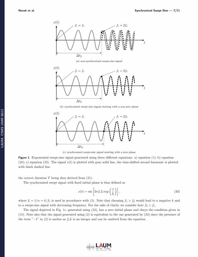
swept-sine signal. This situation is depicted in Fig. 1a, where the exponential swept-sine signal generated using (1)
is not synchronized with its time-shifted second-harmonic copy.
The signal depicted in Fig. 1b, generated using (28), is obviously well synchronized, but the initial phase does
not start at origin. To overcome the initial phase problem while keeping the synchronization correct, we fix the
phase to zero at t = 0, i.e. ϕ(0) = 2πk, that is according to (29)
2πf1T
ln(f2/f1)= 2πk (30)
and we get
k =f1T
ln(f2/f1), (31)
where k ∈ Z6=0. Note that, since k is an integer, the time T and the frequencies f1 and f2 have to be dependent.
In practice, we can define the start frequency f1, the stop frequency f2 and an approximative duration T of the
swept-sine signal. The integer k can then be calculated as
k = round
f1
ln(f2f1
) T , (32)
LA
UM
,C
NR
SU
MR
66
13
Novak et al. Synchronized Swept-Sine — 7/21
(a) non-synchronized swept-sine signal
(b) synchronized swept-sine signal starting with a non-zero phase
(c) synchronized swept-sine signal starting with a zero phase
Figure 1. Exponential swept-sine signal generated using three different equations: a) equation (1); b) equation
(28); c) equation (33). The signal x(t) is plotted with gray solid line, the time-shifted second harmonic is plotted
with black dashed line.
the correct duration T being then derived from (31).
The synchronized swept signal with fixed initial phase is thus defined as
x(t) = sin
[2πf1L exp
(t
L
)], (33)
where L = 1/α = k/f1 is used in accordance with (3). Note that choosing f1 > f2 would lead to a negative k and
to a swept-sine signal with decreasing frequency. For the sake of clarity we consider here f2 > f1.
The signal depicted in Fig. 1c, generated using (33), has a zero initial phase and obeys the condition given in
(18). Note also that the signal generated using (2) is equivalent to the one generated by (33) since the presence of
the term ”−1” in (2) is useless as f1L is an integer and can be omitted from the equation.
LA
UM
,C
NR
SU
MR
66
13

Novak et al. Synchronized Swept-Sine — 8/21
(a) a non-zero final phase at time T ; x(t = T ) 6= 0
(b) a non-zero final phase at time T ; x(t = T ) 6= 0
(c) a zero final phase at time T ; x(t = T ) = 0
Figure 2. The beginning and the end of the exponential swept-sine signal generated using three different equations:
a) equation (1); b) equation (28); c) equation (33). Ending points are highlighted with a black circle.
3.5 Final Phase
The synchronized swept-sine with fixed initial phase defined in (33) has another interesting property concerning
the final phase of the signal. If the final frequency f2 is chosen as an integer multiple of the initial frequency f1,
the phase of the exponential signal x(t) from (33) is zero at the time instant corresponding to the instantaneous
frequency f2. Expressed in other words, the final phase at time T is also zero.
The behavior of the exponential swept-sine signals x(t) near time T is depicted in Fig. 2. The swept-sine
signal generated using (1), depicted in Fig. 2a, exhibits a non-zero final phase at time T . As discussed in [21], the
signal generated by this way should be cut manually at the latest zero-crossing before its abrupt termination. The
synchronized swept-sine with a non-fixed initial phase generated using (28) exhibits a non-zero final phase at time
T . The final phase is, this time, an integer multiple of the initial phase. Finally, the synchronized swept-sine with
fixed initial phase generated using (33) has a zero final phase. Using this approach, we can avoid the manual cut of
the tail of the swept-sine signal.
LA
UM
,C
NR
SU
MR
66
13

Novak et al. Synchronized Swept-Sine — 9/21
Figure 3. Delaying the Synchronized swept-sine signal x(t) = sin[ϕ(t)] by ∆t2 and by ∆t3 is equivalent to
generating the second and third harmonic sin[2ϕ(t)] and sin[3ϕ(t)] of the Synchronized swept-sine signal x(t).
3.6 Time Delays vs. Instantaneous Frequency
The synchronized swept-sine signal generated using (33) has the following property, due to the condition given in
(18). The time-shifted synchronized swept-sine signal by time delay ∆tn is equivalent to the n-th higher harmonic
copy of the signal x(t) itself. The n-th harmonic copy has a phase value, and thus also an instantaneous frequency,
n-times higher than the one of the original synchronized swept-sine signal x(t). This property is depicted in Fig. 3.
The time delays ∆tn can be derived from (22) as
∆tn = L ln(n). (34)
Similarly, the instantaneous frequency fi(t) can be derived from (24) as
fi(t) = f1 exp
(t
L
). (35)
According to the condition given in (18) we can find a simple relation between the instantaneous frequency
fi(t) and the time delays ∆tn. The time delays ∆tn indicate the time instants corresponding to the instantaneous
frequency (and phase) n-times higher than the initial frequency (and phase), which can be written mathematically
as
fi(∆tn) = nf1. (36)
Moreover, thanks to the synchronization of the swept-sine and fixed initial phase, we can write
x(∆tn) = 0. (37)
Both properties are depicted together in Fig. 4.
4. IMPULSE RESPONSE DECONVOLUTION
The previous section discussed the generation of the synchronized swept-sine signal x(t) that is used as the input
to the nonlinear system under test. After the measurement, the output signal y(t) is acquired and the impulse
LA
UM
,C
NR
SU
MR
66
13

Novak et al. Synchronized Swept-Sine — 10/21
Figure 4. Synchronized swept-sine x(t) (below) and the associated instantaneous frequency fi(t).
response consisting of time-delayed higher harmonic impulse responses can be deconvolved from the output signal
y(t). The impulse response deconvolution is usually performed using (4) or (7).
4.1 Analytical Deconvolution
Another way to deconvolve the impulse response h(t) is to use an analytical expression of the inverse filter in the
frequency domain X(f) and then compute the deconvolution directly in the frequency domain as
h(t) = F−1[F [y(t)]X(f)]
]. (38)
In order to derive the Fourier transform of the synchronized swept-sine signal X(f), we use the analytical swept-sine
signal z(t) defined as
z(t) = exp [jϕ(t)] (39)
that, in relation with the swept-sine signal x(t) from Eq. (33), is expressed as
z(t) = xc(t) + jx(t) (40)
where xc(t) = −H[x(t)] is the cosine version of the synchronized swept-sine defined as the negative Hilbert transform
of x(t).
The mathematical derivation of the Fourier transform of the analytical signal z(t) is provided in Appendix A.1
and results in
Z(f) =
√L
fexp
{j2πfL
[1− ln
(f
f1
)]+ j
π
4
}, (41)
from which the Fourier transform of the synchronized swept-sine signalX(f) can be expressed for positive frequencies
LA
UM
,C
NR
SU
MR
66
13

Novak et al. Synchronized Swept-Sine — 11/21
Figure 5. Result of the deconvolution process resulting in a sum of time-shifted higher harmonic impulse responses
hn(t)
f as
X(f) =1
2
√L
fexp
{j2πfL
[1− ln
(f
f1
)]− j π
4
}, (42)
and the Fourier transform of inverse filter X(f) as
X(f) = 2
√f
Lexp
{−j2πfL
[1− ln
(f
f1
)]+ j
π
4
}. (43)
4.2 Group Delay
Lastly, the spectra X(f) from Eq. (42) has a phase such that
φ(f) = 2πfL
[1− ln
(f
f1
)]− π
4, (44)
from which the group delay can be derived according to its definition as
τg(f) = − 1
2π
dφ(f)
df= L ln
(f
f1
). (45)
Note, that the group delay from Eq. (45) is an inverse function to the instantaneous frequency fi(t) defined in
Eq. (35). Because of this property, the signal x(t) is an asymptotic signal [23, 24].
5. HIGHER HARMONICS SEPARATION
The deconvolution process defined in Eq. (38) results in impulse response h(t) which is according to Eq. (12 ) a
sum of time-shifted higher harmonic impulse responses hn(t). A schematic example of the impulse response h(t) is
depicted in Fig. 5.
The higher harmonic impulse responses hn(t) are easy to separate by windowing in the time domain as described
in [19]. Finally, they can be Fourier transformed into frequency domain as
Hn(f) = F [hn(t)] . (46)
The magnitude plot of Hn(f) in decibel units is the most common representation, since it shows the amount of
distortion of all the harmonics as a function of frequency [1].
LA
UM
,C
NR
SU
MR
66
13

Novak et al. Synchronized Swept-Sine — 12/21
Figure 6. Schematic representation of magnitude spectra of HHFRs Hn(f). (a) The deconvolution using
Eqs. (4) or (7) set the upper bandwidth limit to f2. (b) The deconvolution using the analytic expression in
Eq. (38) does not limit the frequency bandwidth of HHFRs.
It is worth noting that using the usual way of deconvolving the impulse response using Eq. (4) or Eq. (7), the
frequency bandwidth of HHFRs is [nf1, f2], where n is the number of studied HHFRs. Consequently, all the HHFRs
stops at frequency f2 as depicted in Fig. 6a.
On the other hand, if we use the deconvolution defined in Eq. (38) which is based on the analytical expression of
the swept-sine signal in frequency domain, the frequency bandwidth of HHFRs is [nf1, nf2] as depicted in Fig. 6b.
In other words, the deconvolution using the analytical expression leads to much larger frequency band of HHFRs.
LA
UM
,C
NR
SU
MR
66
13
Novak et al. Synchronized Swept-Sine — 13/21
6. SUMMARY OF SYNCHRONIZED SWEPT-SINE METHOD
Since we have discussed several ways of generating the exponential swept-sine signal as well as several ways of
deconvolving the impulse response, we shortly summarize, in this section, the main equations for the generation
and the deconvolution that will be used as a theoretical basis for the implementation provided in Sec. A.2.
The synchronized swept-sine is generated using
x(t) = sin
[2πf1L exp
(t
L
)]. (47)
where
L =T
ln(f2f1
) , (48)
and where f1 and f2 are initial and final frequency respectively and T is duration of the swept-sine. Contrary to
previous works [16, 17] no added constraint is imposed on the rate of frequency increase L. However, if the initial
phase is restricted te be zero at time t = 0 the rate of frequency increase L is defined as
L =1
f1round
f1
ln(f2f1
) T , (49)
T being an approximative duration of the swept-sine. In such a case if the final frequency f2 is chosen as an integer
multiple of the initial frequency f1, the synchronized swept-sine ends up with zero phase.
The deconvolution process is next performed in the frequency domain as
h(t) = F−1[F [y(t)]X(f)]
], (50)
where y(t) is the acquired response of the nonlinear system under test to the synchronized swept-sine, and where
the Fourier transform of inverse filter X(f) is
X(f) = 2
√f
Lexp
{−j2πfL
[1− ln
(f
f1
)]+ j
π
4
}. (51)
The impulse response h(t) then consist of time-delayed higher harmonic impulse responses separated by time delays
∆tn = L ln(n). (52)
A full Matlab code, including all the necessary steps to implement the method is provided in appendix A.2.
7. Illustrative Example
In order to illustrate the advantage of using the synchronized swept-sine signal instead of the non-synchronized
swept-sine signal for the estimation of the HHFRs, we present in this section the results of an experiment performed
on a woofer (Pioneer W16FU90-51H). The woofer is excited using both the exponential (non-synchronized) swept-
sine signal (1), called ESS, and the synchronized swept-sine signal (33), called SSS. The HHFRs of distorted current
running through the woofer are estimated and compared with a measurement performed with a harmonic signal.
The measurement is performed using the sampling frequency fs = 50 kHz. The parameters of the synchronized
swept-sine signal are: the initial frequency f1 = 5 Hz; the final frequency f2 = 500 Hz; and the approximative time
duration T = 10 s. The amplitude of both excitation signals is 5 V rms, high enough to produce distortion artifacts
on the current.
LA
UM
,C
NR
SU
MR
66
13

Novak et al. Synchronized Swept-Sine — 14/21
101
102
−70
−60
−50
−40
−30
−20
−10
0
frequency [Hz]
Cu
rre
nt
Sp
ectr
a [
dB
]1
st harmonic
2nd
harmonic
3rd
harmonic
101
102
−1
−0.5
0
0.5
11
st harmonic
frequency [Hz]
ph
ase
[ra
d]
101
102
−4
−2
0
2
42
nd harmonic
frequency [Hz]
ph
ase
[ra
d]
101
102
−4
−2
0
2
43
rd harmonic
frequency [Hz]
ph
ase
[ra
d]
SSS method
ESS method
sine step−by−step
SSS method
ESS method
sine step−by−step
SSS method
ESS method
sine step−by−step
SSS method
ESS method
sine step−by−step
Figure 7. First three HHFRs of the distorted current passing through the woofer estimated using the
non-synchronized swept-sine signal ESS (dashed line) and the synchronized swept-sine signal SSS (gray line),
compared with a step-by-step measurement using a sine-wave excitation (dots).
The amplitudes and phases of the first three HHFRs estimated using both versions of exponential swept-sine
signal are depicted in Fig. 7 and are compared with a measurement performed with a harmonic signal, the frequency
of which is changed step-by-step from 10 to 100 Hz with a 10 Hz step. Whilst the amplitudes of all the HHFRs are
correctly estimated for all the harmonics, the phases of the HHFRs Hn(f) (n > 1) are wrongly estimated in the
case of the non-synchronized swept-sine signal (ESS). The reason for this error is the non-synchronization of the
swept-sine signal as described in previous sections.
The harmonic phases presented in Fig. 7 are the phases of hn(t) related to the system under test and should be
independent on the input signal x(t). However, if the swept-sine signal is not correctly synchronized, the phases
of hn(t) become dependent on the input signal x(t) which is undesirable. On the other hand, if the swept-sine
signal is correctly synchronized the phases of hn(t) remain independent on the input signal x(t). This is confirmed
in the illustrative example in Fig. 7, where the phases of all the HHFRs are correctly estimated in the case of the
synchronized swept-sine (SSS).
8. CONCLUSION
In this paper, the theory of Synchronized Swept-Sine method has been revised. It has been shown that for a correct
generation of the synchronized swept-sine a specific formula has to be used. Otherwise, the exponential swept-sine
signal is not synchronized leading to an incorrect estimation of phases of Higher Harmonic Frequency Responses.
If the synchronized swept-sine is generated using the equation derived in this paper the phases of Higher Harmonic
LA
UM
,C
NR
SU
MR
66
13

Novak et al. Synchronized Swept-Sine — 15/21
Frequency Responses are correctly estimated.
Moreover, the analytical formula for the spectra of the synchronized swept-sine has been derived. Thus, the
deconvolution of the impulse response can be made directly in the frequency domain using the analytical expression.
Advantage of using the deconvolution with the analytical formula is that the estimated Higher Harmonic Frequency
Responses have larger frequency bandwidth than when deconvolved the usual way. The use of analytical formula
for the deconvolution is also less time consuming.
We have illustrated the advantages of using a synchronized swept-sine method over the usual non-synchronized
one on analysis of current distortion of a woofer. Moreover, some application issues of the implementation are
discussed in Appendix including a full Matlab code of the method.
References
[1] A. Farina, “Simultaneous measurement of impulse response and distortion with a swept-sine technique,” in
AES 108th convention, (Paris), Feb. 2000.
[2] A. Farina, A. Bellini, and E. Armelloni, “Non-linear convolution: A new approach for the auralization of
distorting systems,” in AES 110th convention, (Amsterdam), May 2001.
[3] P. G. Craven and M. A. Gerzon, “Practical adaptive room and loudspeaker equaliser for hi-fi use,” in Audio
Engineering Society Conference: UK 7th Conference: Digital Signal Processing (DSP), Audio Engineering
Society, 1992.
[4] D. Griesinger, “Beyond mls-occupied hall measurement with fft techniques,” in Audio Engineering Society
Convention 101, Audio Engineering Society, 1996.
[5] J. O. Jungmann, R. Mazur, M. Kallinger, T. Mei, and A. Mertins, “Combined acoustic mimo channel crosstalk
cancellation and room impulse response reshaping,” Audio, Speech, and Language Processing, IEEE Transac-
tions on, vol. 20, no. 6, pp. 1829–1842, 2012.
[6] D. G. Ciric, M. Markovic, M. Mijic, and D. Sumarac-Pavlovic, “On the effects of nonlinearities in room impulse
response measurements with exponential sweeps,” Applied Acoustics, vol. 74, no. 3, pp. 375–382, 2013.
[7] P. Majdak, P. Balazs, and B. Laback, “Multiple exponential sweep method for fast measurement of head-related
transfer functions,” Journal of the Audio Engineering Society, vol. 55, no. 7/8, pp. 623–637, 2007.
[8] P. Dietrich, B. Masiero, and M. Vorlander, “On the optimization of the multiple exponential sweep method,”
Journal of the Audio Engineering Society, vol. 61, no. 3, pp. 113–124, 2013.
[9] A. Novak, M. Bentahar, V. Tournat, R. El Guerjouma, and L. Simon, “Nonlinear acoustic characterization of
micro-damaged materials through higher harmonic resonance analysis,” NDT & E International, vol. 45, no. 1,
pp. 1–8, 2012.
[10] J. Legland, V. Tournat, O. Dazel, A. Novak, and V. Gusev, “Linear and nonlinear biot waves in a noncohe-
sive granular medium slab: Transfer function, self-action, second harmonic generation,” The Journal of the
Acoustical Society of America, vol. 131, no. 6, pp. 4292–4303, 2012.
[11] G.-B. Stan, J.-J. Embrechts, and D. Archambeau, “Comparison of different impulse response measurement
techniques,” Journal of the Audio Engineering Society, vol. 50, no. 4, pp. 249–262, 2002.
[12] S. Bilbao and J. Parker, “A virtual model of spring reverberation,” Audio, Speech, and Language Processing,
IEEE Transactions on, vol. 18, no. 4, pp. 799–808, 2010.
LA
UM
,C
NR
SU
MR
66
13

Novak et al. Synchronized Swept-Sine — 16/21
[13] J. Kemp and H. Primack, “Impulse response measurement of nonlinear systems: Properties of existing tech-
niques and wide noise sequences,” Journal of the Audio Engineering Society, vol. 59, no. 12, pp. 953–963,
2012.
[14] A. Benichoux, L. Simon, and R. Gribonval, “Convex regularizations for the simultaneous recording of room
impulse responses,” Signal Processing, IEEE Transactions on, vol. 62, no. 8, pp. 1976 – 1986, 2014.
[15] A. Novak, L. Simon, P. Lotton, and F. Kadlec, “A new method for identification of nonlinear systems using
miso model with swept-sine technique: Application to loudspeaker analysis,” in Audio Engineering Society
Convention 124, Audio Engineering Society, May 2008.
[16] A. Novak, L. Simon, F. Kadlec, and P. Lotton, “Nonlinear system identification using exponential swept-sine
signal,” Instrumentation and Measurement, IEEE Transactions on, vol. 59, no. 8, pp. 2220–2229, 2010.
[17] M. Rebillat, R. Hennequin, E. Corteel, and B. F. Katz, “Identification of cascade of hammerstein models
for the description of nonlinearities in vibrating devices,” Journal of Sound and Vibration, vol. 330, no. 5,
pp. 1018–1038, 2011.
[18] A. Novak, B. Maillou, P. Lotton, and L. Simon, “Nonparametric identification of nonlinear systems in series,”
Instrumentation and Measurement, IEEE Transactions on, vol. 63, no. 8, pp. 2044–2051, 2014.
[19] S. Muller and P. Massarani, “Transfer-function measurement with sweeps,” Journal of the Audio Engineering
Society, vol. 49, no. 6, pp. 443–471, 2001.
[20] L. Tronchin, “The emulation of nonlinear time-invariant audio systems with memory by means of volterra
series,” Journal of the Audio Engineering Society, vol. 60, no. 12, pp. 984–996, 2013.
[21] A. Farina, “Advancements in impulse response measurements by sine sweeps,” in Audio Engineering Society
Convention 122, Audio Engineering Society, May 2007.
[22] T. Erneux, Applied delay differential equations, vol. 3. Springer, 2009.
[23] B. Boashash, “Estimating and interpreting the instantaneous frequency of a signal. i. fundamentals,” Proceed-
ings of the IEEE, vol. 80, no. 4, pp. 520–538, 1992.
[24] L. Cohen, “Instantaneous frequency and group delay of a filtered signal,” Journal of the Franklin Institute,
vol. 337, no. 4, pp. 329–346, 2000.
[25] J. R. Carson and T. C. Fry, “Variable frequency electric circuit theory with application to the theory of
frequency-modulation,” Bell System Technical Journal, vol. 16, no. 4, pp. 513–540, 1937.
[26] C. E. Cook, Radar Signals: An Introduction to Theory and Application. Academic Press, 1967.
[27] M. Garai and P. Guidorzi, “Optimizing the exponential sine sweep (ess) signal for in situ measurements on
noise barriers,” in Euronoise 2015, EAA, Euronoise.
[28] A. V. Oppenheim, R. W. Schafer, J. R. Buck, et al., Discrete-time signal processing, vol. 2. Prentice-hall
Englewood Cliffs, 1989.
[29] A. Torras-Rosell and F. Jacobsen, “A new interpretation of distortion artifacts in sweep measurements,” Journal
of the Audio Engineering Society, vol. 59, no. 5, pp. 283–289, 2011.
LA
UM
,C
NR
SU
MR
66
13

Novak et al. Synchronized Swept-Sine — 17/21
APPENDIX
A.1 Fourier Transform of the Synchronized Swept-Sine Signal
The Fourier transform of the analytical signal z(t) from Eq. (39) is defined as
Z(f) =
∞∫−∞
z(t) exp (−j2πft) dt (A.1)
=
∞∫−∞
exp
{j2π
[Lf1 exp
(t
L
)− ft
]}dt, (A.2)
which can be expressed as
Z(f) =
∞∫−∞
exp (j2πΘ(t)) dt, (A.3)
where
Θ(t) = Lf1 exp
(t
L
)− ft (A.4)
is the phase of the exponential term. The function Θ(t) is a convex function with a global minimum at
tk = L ln
(f
f1
). (A.5)
Note, that this equation is the same as the one defining the group delay (45).
In order to find the Fourier transform defined in Eq. (A.1), we express the phase Θ(t) in a Taylor series around
the time tk for each frequency f as
Θ(t) =
∞∑n=0
Θ(n)(tk)
n!(t− tk)n. (A.6)
We first solve all the derivatives Θ(n)(t)
Θ(t) = Lf1 exp
(t
L
)− ft, (A.7)
Θ′(t) = f1 exp
(t
L
)− f, (A.8)
Θ(n)(t) =f1
Ln−1exp
(t
L
), (n ≥ 2) (A.9)
and then we solve them for tk from Eq. (A.5)
Θ(tk) = Lf − fL ln(f
f1), (A.10)
Θ′(tk) = f − f = 0, (A.11)
Θ(n)(tk) =f
Ln−1, (n ≥ 2). (A.12)
The Taylor series from (A.6) can be then expressed as
Θ(t) = Lf − fL ln
(f
f1
)+
∞∑n=2
f
L(n−1)n!(t− tk)n. (A.13)
LA
UM
,C
NR
SU
MR
66
13

Novak et al. Synchronized Swept-Sine — 18/21
Putting the phase (A.13) to the Fourier transform (A.3) and using the principle of stationary phase [25, 26] allowing
us to neglect the terms n > 2 in (A.13) we can write
Z(f) = exp
{j2πfL
[1− ln
(f
f1
)]}
×∞∫−∞
exp
[jπf
(t− tk)2
L
]dt. (A.14)
Substituting u = t− tk we get the function inside the integral even, leading to
Z(f) = exp
{j2πfL
[1− ln
(f
f1
)]}
×2
∞∫0
exp
[jπf
u2
L
]du. (A.15)
The integral in Eq. (A.15) is one form of the Fresnel integral. Finally, solving the Fresnel integral we can write
Z(f) = exp
{j2πfL
[1− ln
(f
f1
)]}×
√L
fexp(j
π
4). (A.16)
A.2 IMPLEMENTATION AND APPLICATION
The application and implementation issues of the proposed method are discussed in this section. A Matlab code is
provided for each important step.
A.2.1 Synchronized Swept-Sine Signal Generation
The first step is the generation of the synchronized swept-sine signal. We first define the initial, final and sampling
frequency and the time duration of the swept-sine signal.
1 f1 = 5; % initial frequency
2 f2 = 500; % final frequency
3 fs = 50000; % sampling frequency
4 T = 10; % time duration
The choice of these parameters should be suited to the nonlinear system under test. In the example given in Sec. 7
we analyzed the current distortion of a woofer using an acquisition system with sampling frequency fs = 50 kHz.
Since the current distortion of a woofer is most important at very low frequencies we set the frequency range between
f1 = 5 Hz and f2 = 500 Hz.
Next, we generate the signal using Eqs. (47) and (49)
1 L = T/log(f2/f1);
2 t = (0:ceil(fs*T)−1)./fs;3 x = sin(2*pi*f1*L*(exp(t/L))).';
A.2.2 Windowing, fade-in and fade-out
For some applications it might be useful to apply a fade-in and/or fade-out window on the input signal [21, 27]. In
[27], an optimal length and shape of these two windows is discussed. In the following code we propose a so-called
raised cosine window [28], but any kind of window can be used [27].
LA
UM
,C
NR
SU
MR
66
13

Novak et al. Synchronized Swept-Sine — 19/21
1 % fade−in the input signal
2 fd1 = 4800; % number of samlpes
3 fade in = (1−cos((0:fd1−1)/fd1*pi))/2;4 index = 1:fd1;
5 x(index) = x(index).*fade in.';
6
7 % fade−out the input signal
8 fd2 = 4800; % number of samlpes
9 fade out = (1−cos((0:fd2−1)/fd2*pi))/2;10 index = (1:fd2)−1;11 x(end−index) = x(end−index).*fade out.';
Note, that if we perform the deconvolution using (4) or (7) that applies the generated input signal data x(t) to
calculate the inverse filter, the fade-in fade-out windows are applied twice: once to the input signal x(t) and once
to the inverse filter. On the other hand, when the analytical formula for deconvolution (38) is used, the fading
windows are applied only to the input signal x(t).
A.2.3 Output signal and its DC Component Filtration
Once the synchronized swept sine signal is generated it can be used as the excitation to the nonlinear system under
test. As discussed in [1], it is common to add a segment of silence after the excitation signal in order to avoid the
cut of the tail of the systems response. In the following, we suppose the output signal y(t) of the nonlinear system
was correctly recorder and saved in Matlab under a variable y (a column).
It may happen that after recording the system response y(t) the latter contains a DC component or even
some very low-frequency content. This is either due to the nonlinear system under test itself [29], or due to the
measurement setup, for example a vibrometer measuring a displacement signal may already be in a DC off-set. In
both cases, the DC component should be filtered-out from the signal, otherwise it can contaminate the deconvolved
impulse response with the scaled inverse filter x(t) as shown below.
Let call the output signal with no DC component y(t) and the DC component of the signal as yDC so the
recorder signal may be in form of y(t) + yDC . When convolving this signal with the inverse filter x(t), it will result
in(y(t) + yDC) ∗ x(t) = y(t) ∗ x(t) + yDC · x(t)
= h(t) + yDC · x(t).(A.17)
Note, that the output of the deconvolution is the desired impulse response h(t) plus an undesired inverse filter x(t)
scaled by the yDC factor.
Thus, the DC component must be filtered out either electrically (many of Digital-to-Analog Converters have a
protective high-pass filter implemented on chip), or by doing it manually. Once the DC component filtered-out, the
deconvolution of the impulse response can be carried out.
A.2.4 Deconvolution
The deconvolution in frequency domain is implemented using Eq. (50) and the analytical expression of the inverse
filter in frequency domain from Eq. (51).
1 % Output signal spectra
2 len = 2ˆceil(log2(length(y)));
3 Y = fft(y,len)./fs; % FFT of y
4
5 % frequency axis
6 f ax = linspace(0,fs,len+1).';
LA
UM
,C
NR
SU
MR
66
13

Novak et al. Synchronized Swept-Sine — 20/21
Figure 8. Schematic representation of time delay ∆t4 being between two samples of sampled impulse response h(t).
7 f ax = f ax(1:end−1);8
9 % inverse filter in frequency domain
10 X = 2*sqrt(f ax/L).*exp(−j*2*pi* ...
11 f ax*L.*(1−log(f ax/f1)) + j*pi/4);
12
13 % Deconvolution
14 H = Y.*X ;
15 H(1) = 0; % avoid Inf at DC
16
17 % higher harmonic impulse responses
18 h = ifft(H,'symmetric');
A.2.5 Separation of Higher Harmonic Impulse Responses
The deconvolution process results in the impulse response, that consists of time-delayed sum of higher harmonic
impulse responses as depicted in Fig. 5. In order to separate them from each other, we must first calculate the
time-moments ∆tn in which these higher harmonic impulse responses appear using Eq. (52). In order to obtain
directly the number of samples by which the higher harmonic impulse responses are shifted, we multiply the time
delays ∆tn by the sampling frequency fs.
1 N = 3; % number of higher harmonics
2 % positions of higher harmonic IRs
3 dt = L.*log(1:N).*fs;
However, the number of samples dt defined as ∆tnfs is not necessarily an integer number leading to a non-integer
sample shift to be realized. A schematic example of such a situation is depicted in Fig. 8. Thus, we first separate
the higher harmonic impulse responses at the integer shift calculated as the rounded version of the exact non-integer
number of samples and, after the separation, we implement the non-integer delay in frequency domain using the
time shift property of the Fourier transform
F [f(t− t0)] = exp(−jωt0)F [f(t)] . (A.18)
LA
UM
,C
NR
SU
MR
66
13

Novak et al. Synchronized Swept-Sine — 21/21
Finally, the HHFRs Hn(f) are calculated as the Fourier transform of the higher harmonic impulse responses hn(t).
1 % Length of each IR (in samples)
2 len IR = 2ˆ12;
3 half IR = round(len IR/2);
4
5 % rounded positions [samples]
6 dt = round(dt);
7 % non−integer difference
8 dt rem = dt − dt ;
9
10 % circular periodisation of IR
11 h pos = [h; h(1:half IR + len IR)];
12
13 % frequency axis definition
14 axe w = linspace(0,2*pi,len IR+1).';
15 axe w = axe w(1:end−1);16
17 % space localisation for IRs
18 hs = zeros(len IR,N);
19
20 for n = 1:N
21 % start position of n−th IR
22 st = len−dt (n)−half IR;
23
24 % separation of IRs
25 hs(:,n) = h pos(st:st+len IR−1);26
27 % apply windowing if needed
28
29 % Non−integer sample delay
30 Hx = fft(hs(:,n)).* ...
31 exp(−j*dt rem(n)*axe w);
32 hs(:,n) = ifft(Hx,'symmetric');
33 end
34
35 % Higher Harmonic Frequency Responses
36 Hs = fft(hs);
To smooth out the transitions between the impulse responses hn(t) and to control spectral ripples and time
non-casual spreads, the impulse responses can be tapered prior to truncation using window functions such as the
Hamming, the Bartlett, or the Kaizer windows [28].
LA
UM
,C
NR
SU
MR
66
13