synchronization architecture in parallel programming modelsarturo/ftp/th_slides.pdf · arturo...
TRANSCRIPT

Synchronization Architecture
in Parallel Programming Models
PhD Thesis
Arturo Gonz alez Escribano
Supervisors: Valentın Cardenoso Payo (Univ. Valladolid)Arie J.C. van Gemund (TU Delft) July, 2003
1
Conceptual approach and models review
Introduction
Experimental approach
Theoretical and algorithmic approach
Conclusion
Outline
2
Intr
od
uct
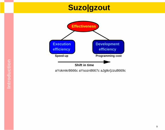
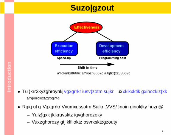
ionMotivation
Speed-up Programming cost
Shift in time
Developmentefficiency
Executionefficiency
Effectiveness
[Siegel2000] [Smith2001] [Danelutto2003]
3

Intr
od
uct
ionMotivation
Speed-up Programming cost
Shift in time
Developmentefficiency
Executionefficiency
Effectiveness
[Siegel2000] [Smith2001] [Danelutto2003]
• No well-established parallel computing model or reference architecture[SkillicornTalia98]
3
Intr
od
uct
ionMotivation
Speed-up Programming cost
Shift in time
Developmentefficiency
Executionefficiency
Effectiveness
[Siegel2000] [Smith2001] [Danelutto2003]
• No well-established parallel computing model or reference architecture[SkillicornTalia98]
• Lack of a Parallel Programming Model (PPM) which achieves both:
– Software development capabilities
– Portability and efficient implementations
3

Intr
od
uct
ion
Parallel systems modeling challengesExisting approaches
4
Intr
od
uct
ion
Parallel systems modeling challengesExisting approaches
• High abstract level
+ Elegant semantic models– Complex specifications– Too far from lower level details for easy implementation
4
Intr
od
uct
ion
Parallel systems modeling challengesExisting approaches
• High abstract level
+ Elegant semantic models– Complex specifications– Too far from lower level details for easy implementation
• Focused on the low level details
+ Allow to exploit all parallelism power– Difficult to program, analyze and debug
• Restricted models
– Reduce the expressive power+ Simple & analyzable structures
The expressive power and analyzability of a modelappear to be highly related to communication/synchronization
4
Intr
od
uct
ion
SA
• We coin the term Synchronization Architecture (SA) to summarizethe formal description of communication & synchronization logicstructures
5
Intr
od
uct
ion
SA
• We coin the term Synchronization Architecture (SA) to summarizethe formal description of communication & synchronization logicstructures
• Why architecture?
– Description of synchronization/communication mechanisms
– Description of the composition rules
5

Intr
od
uct
ion
SA
• We coin the term Synchronization Architecture (SA) to summarizethe formal description of communication & synchronization logicstructures
• Why architecture?
– Description of synchronization/communication mechanisms
– Description of the composition rules
• Why synchronization?
– Generalization of both communication & synchronization
5
Intr
od
uct
ion
SA
• We coin the term Synchronization Architecture (SA) to summarizethe formal description of communication & synchronization logicstructures
• Why architecture?
– Description of synchronization/communication mechanisms
– Description of the composition rules
• Why synchronization?
– Generalization of both communication & synchronization
– Synchronization and computation are orthogonal[GelernterCarriero92]
– Synchronization distinguishes parallel from sequential solutions
5

Intr
od
uct
ion
Problem statement
• What is the relationship between SA and properties of PPMs?We propose a new classification system for PPMs
6
Intr
od
uct
ion
Problem statement
• What is the relationship between SA and properties of PPMs?We propose a new classification system for PPMs
• What are the advantages and drawbacks of restricted SAs?We show that one SA class, called SP, groups the most interesting models
6
Intr
od
uct
ion
Problem statement
• What is the relationship between SA and properties of PPMs?We propose a new classification system for PPMs
• What are the advantages and drawbacks of restricted SAs?We show that one SA class, called SP, groups the most interesting models
• How is expressive power affected by the restriction?We present systematic transformation methods to map non-SP applications into SP form
We investigate the potential performance impact of these transformations
We will show that SP PPMs bring a good trade-off betweenexpressive power and analyzability, being a good choice forgeneral-purpose parallel computing
6

Intr
od
uct
ionApproach
Three-step approach
7
Intr
od
uct
ionApproach
Three-step approach
• Conceptual
– SA classification– Review of models at different abstraction levels– Relate SA to PPM characteristics– Detect which applications naturally map to each class
7
Intr
od
uct
ionApproach
Three-step approach
• Conceptual
– SA classification– Review of models at different abstraction levels– Relate SA to PPM characteristics– Detect which applications naturally map to each class
• Theoretical
– SP graph characterization– NSP to SP transformation (algorithmic) techniques– Potential performance loss study
• Experimental
– Graph modeling of applications– Experiments with synthetic graphs– Experiments with real application graphs
7
Co
nce
ptu
alSA classification criteria
8

Co
nce
ptu
alSA classification criteria
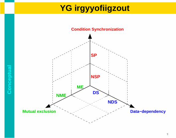
• Two main types of synchronization [AndrewsSchneider82]
8
Co
nce
ptu
alSA classification criteria
• Two main types of synchronization [AndrewsSchneider82]
– Condition synchronization (CS)
∗ Communications or event synchronization∗ Implies an execution order
8
Co
nce
ptu
alSA classification criteria
• Two main types of synchronization [AndrewsSchneider82]
– Condition synchronization (CS)
∗ Communications or event synchronization∗ Implies an execution order
– Mutual Exclusion (ME)
∗ No concurrent execution, but order is not predefined∗ Final order selection is delayed for lower-level optimization
– Orthogonality: A PPM may support one or both of them
• Classes:
– ME axis: ME vs. NME
8

Co
nce
ptu
alSA classification criteria
• Two main types of synchronization [AndrewsSchneider82]
– Condition synchronization (CS)
∗ Communications or event synchronization∗ Implies an execution order
– Mutual Exclusion (ME)
∗ No concurrent execution, but order is not predefined∗ Final order selection is delayed for lower-level optimization
– Orthogonality: A PPM may support one or both of them
• Classes:
– ME axis: ME vs. NME
– CS axis: SP (nested-parallelism, cobegin-coend) vs. NSP
8
Co
nce
ptu
alSA classification criteria
• Two main types of synchronization [AndrewsSchneider82]
– Condition synchronization (CS)
∗ Communications or event synchronization∗ Implies an execution order
– Mutual Exclusion (ME)
∗ No concurrent execution, but order is not predefined∗ Final order selection is delayed for lower-level optimization
– Orthogonality: A PPM may support one or both of them
• Classes:
– ME axis: ME vs. NME
– CS axis: SP (nested-parallelism, cobegin-coend) vs. NSP
• Data-dependent or dynamic structures (DS)
– Dynamic conditions and data-dependent synchronizations
– Impact on analyzability properties [SkillicornTalia98]
– DS axis: DS vs. NDS8
Co
nce
ptu
alSA classification
Condition Synchronization
Mutual exclusion Data−dependency
ME
NMENDS
DS
SP
NSP
9
Co
nce
ptu
alSA classification
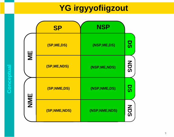
NSPSPM
EN
ME
DS
ND
SD
SD
SN
DS
(SP,ME,DS)
(SP,NME,DS)
(SP,ME,NDS)
(SP,NME,NDS) (NSP,NME,NDS)
(NSP,NME,DS)
(NSP,ME,DS)
(NSP,ME,NDS)
9

Co
nce
ptu
alSA classification
NSPSPM
EN
ME
DS
ND
SD
SD
SN
DS
Restri
ctio
ns
9

Co
nce
ptu
alModel requirements
10
Co
nce
ptu
alModel requirements
• Requirements[SkillicornTalia98]
10
Co
nce
ptu
alModel requirements
• Requirements[SkillicornTalia98]
1 Easy to program2 Software development technology3 Easy to understand4 Architecture independent5 Cost measures6 Guaranteed performance
10
Co
nce
ptu
alModel requirements
• Requirements[SkillicornTalia98]
1 Easy to program2 Software development technology3 Easy to understand4 Architecture independent5 Cost measures6 Guaranteed performance
10

Co
nce
ptu
alModel requirements
• Requirements[SkillicornTalia98]
1 Easy to program2 Software development technology3 Easy to understand4 Architecture independent5 Cost measures6 Guaranteed performance
10
Co
nce
ptu
alModel requirements
• Requirements[SkillicornTalia98]
1 Easy to program2 Software development technology3 Easy to understand4 Architecture independent5 Cost measures6 Guaranteed performance
• Qualitative and difficult to measure
10
Co
nce
ptu
alModel requirements
• Requirements[SkillicornTalia98]
1 Easy to program2 Software development technology3 Easy to understand4 Architecture independent5 Cost measures6 Guaranteed performance
• Qualitative and difficult to measure
• Quantitative study of performance is possible [JuurlinkWijshof98]
• In this work:
– Review of models to determine adequacy and relate it to SA
– For the most relevant SA classes, comparative performance study
10
Co
nce
ptu
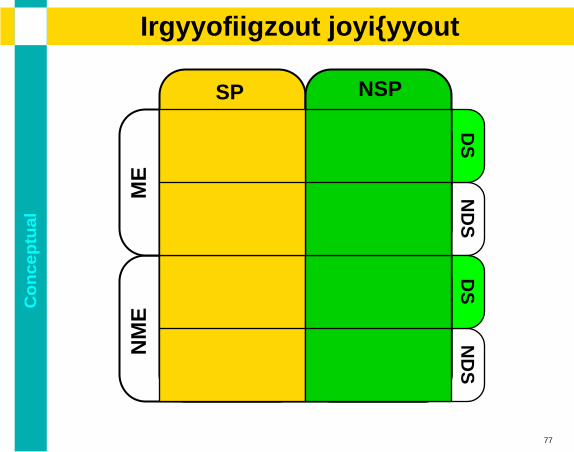
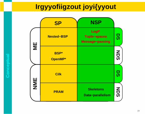
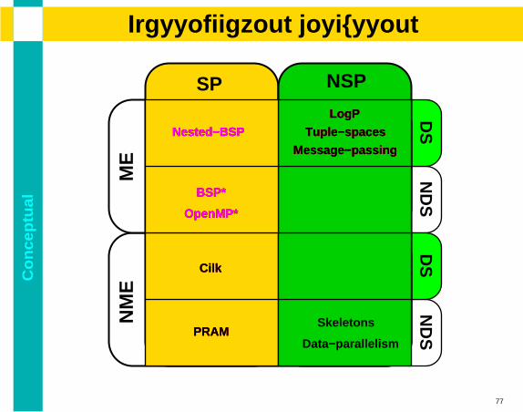
alClassification discussion
ND
SN
DS
DS
DS
ME
NM
E
SP NSP
11

Co
nce
ptu
alClassification discussion
ND
SN
DS
DS
DS
ME
NM
E
SP NSP
PRAM
OpenMP*
LogP
Tuple−spaces
Message−passing
Nested−BSP
BSP*
Cilk
Skeletons
Data−parallelism
11
Co
nce
ptu
alClassification discussion
ND
SN
DS
DS
DS
ME
NM
E
SP NSP
PRAM
OpenMP*
LogP
Tuple−spaces
Message−passing
Nested−BSP
BSP*
Cilk
Skeletons
Data−parallelism
LogP
Tuple−spaces
Message−passing
11

Co
nce
ptu
alClassification discussion
ND
SN
DS
DS
DS
ME
NM
E
SP NSP
PRAM
OpenMP*
LogP
Tuple−spaces
Message−passing
Nested−BSP
BSP*
Cilk
Skeletons
Data−parallelism
LogP
Tuple−spaces
Message−passing
OpenMP*
PRAM
LogP
Tuple−spaces
Message−passing
Nested−BSP
BSP*
Cilk
11
Co
nce
ptu
alClassification discussion
ND
SN
DS
DS
DS
ME
NM
E
SP NSP
PRAM
OpenMP*
LogP
Tuple−spaces
Message−passing
Nested−BSP
BSP*
Cilk
Skeletons
Data−parallelism
LogP
Tuple−spaces
Message−passing
OpenMP*
PRAM
LogP
Tuple−spaces
Message−passing
Nested−BSP
BSP*
Cilk
PRAM
OpenMP*
Nested−BSP
BSP*
Cilk
11

Co
nce
ptu
alClassification discussion
ND
SN
DS
DS
DS
ME
NM
E
SP NSP
PRAM
OpenMP*
LogP
Tuple−spaces
Message−passing
Nested−BSP
BSP*
Cilk
Skeletons
Data−parallelism
LogP
Tuple−spaces
Message−passing
OpenMP*
PRAM
LogP
Tuple−spaces
Message−passing
Nested−BSP
BSP*
Cilk
PRAM
OpenMP*
Nested−BSP
BSP*
Cilk
OpenMP*
Nested−BSP
BSP*
Cilk
11

Co
nce
ptu
alClassification discussion
ND
SN
DS
DS
DS
ME
NM
E
SP NSP
PRAM
OpenMP*
LogP
Tuple−spaces
Message−passing
Nested−BSP
BSP*
Cilk
Skeletons
Data−parallelism
LogP
Tuple−spaces
Message−passing
OpenMP*
PRAM
LogP
Tuple−spaces
Message−passing
Nested−BSP
BSP*
Cilk
PRAM
OpenMP*
Nested−BSP
BSP*
Cilk
OpenMP*
Nested−BSP
BSP*
CilkCilk
Skeletons
Data−parallelism
Skeletons
11
Co
nce
ptu
alConceptual approach summary
• The SA classification is an adequate categorization of PPMs
12
Co
nce
ptu
alConceptual approach summary
• The SA classification is an adequate categorization of PPMs
• The most adequate models are in the SP class
12
Co
nce
ptu
alConceptual approach summary
• The SA classification is an adequate categorization of PPMs
• The most adequate models are in the SP class
• Study of applications [Dissertation 2.6]
12
Co
nce
ptu
alConceptual approach summary
• The SA classification is an adequate categorization of PPMs
• The most adequate models are in the SP class
• Study of applications [Dissertation 2.6]
– Many typical applications naturally map to SP
– Some important classes do not!
12
Co
nce
ptu
alConceptual approach summary
• The SA classification is an adequate categorization of PPMs
• The most adequate models are in the SP class
• Study of applications [Dissertation 2.6]
– Many typical applications naturally map to SP
– Some important classes do not!
• Map NSP applications to SP form:
12
Co
nce
ptu
alConceptual approach summary
• The SA classification is an adequate categorization of PPMs
• The most adequate models are in the SP class
• Study of applications [Dissertation 2.6]
– Many typical applications naturally map to SP
– Some important classes do not!
• Map NSP applications to SP form:Transformations
12
Co
nce
ptu
alConceptual approach summary
• The SA classification is an adequate categorization of PPMs
• The most adequate models are in the SP class
• Study of applications [Dissertation 2.6]
– Many typical applications naturally map to SP
– Some important classes do not!
• Map NSP applications to SP form:Transformations⇒ Performance loss
12
Co
nce
ptu
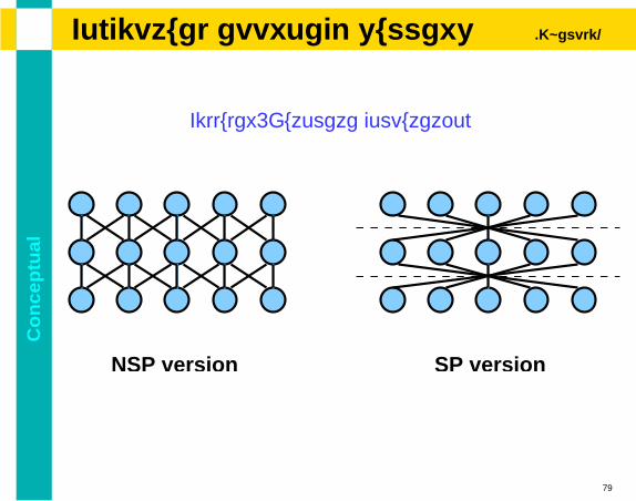
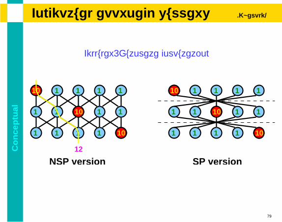
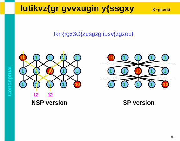
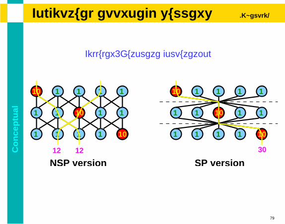
alConceptual approach summary (Example)
Cellular-Automata computation
13
Co
nce
ptu
alConceptual approach summary (Example)
Cellular-Automata computation
NSP version
13
Co
nce
ptu
alConceptual approach summary (Example)
Cellular-Automata computation
NSP version SP version
13
Co
nce
ptu
alConceptual approach summary (Example)
Cellular-Automata computation
NSP version SP version
13
Co
nce
ptu
alConceptual approach summary (Example)
Cellular-Automata computation
NSP version SP version
13
Co
nce
ptu
alConceptual approach summary (Example)
Cellular-Automata computation
NSP version SP version
10
10
10
10
10
10
1 1 11
1
1 1
1
1
1 1
1 1 1 1 1
1 1
1111
11
13
Co
nce
ptu
alConceptual approach summary (Example)
Cellular-Automata computation
NSP version SP version
10
10
10
10
10
10
1 1 11
1
1 1
1
1
1 1
1 1 1 1 1
1 1
1111
11
12
13
Co
nce
ptu
alConceptual approach summary (Example)
Cellular-Automata computation
NSP version SP version
10
10
10
10
10
10
1 1 11
1
1 1
1
1
1 1
1 1 1 1 1
1 1
1111
11
1212
13
Co
nce
ptu
alConceptual approach summary (Example)
Cellular-Automata computation
NSP version SP version
10
10
10
10
10
10
1 1 11
1
1 1
1
1
1 1
1 1 1 1 1
1 1
1111
11
1212 30
13
Co
nce
ptu
alConceptual approach summary (Example)
Cellular-Automata computation
NSP version SP version
10
10
10
10
10
10
1 1 11
1
1 1
1
1
1 1
1 1 1 1 1
1 1
1111
11
1212 30
It is necessary to study the transformations: NSP→ SPand their potential performance impact
13
Th
eore
tica
lTheoretical approach
Graphs
14
Th
eore
tica
lTheoretical approach
Graphs
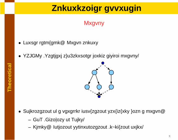
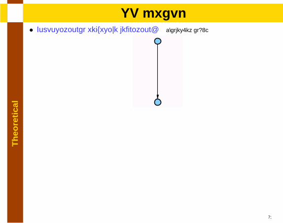
• Formal language: Graph theory
14
Th
eore
tica
lTheoretical approach
Graphs
• Formal language: Graph theory
• STDAGs (Standard two-terminal direct acyclic graphs)
14
Th
eore
tica
lTheoretical approach
Graphs
• Formal language: Graph theory
• STDAGs (Standard two-terminal direct acyclic graphs)
14

Th
eore
tica
lTheoretical approach
Graphs
• Formal language: Graph theory
• STDAGs (Standard two-terminal direct acyclic graphs)
14
Th
eore
tica
lTheoretical approach
Graphs
• Formal language: Graph theory
• STDAGs (Standard two-terminal direct acyclic graphs)
• Modelization of a parallel computation structures with a graph:
– AoN (Activity on Nodes)
– Edges: Condition synchronization (execution order)
14

Th
eore
tica
lSP graph
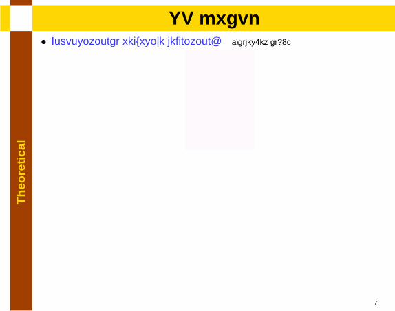
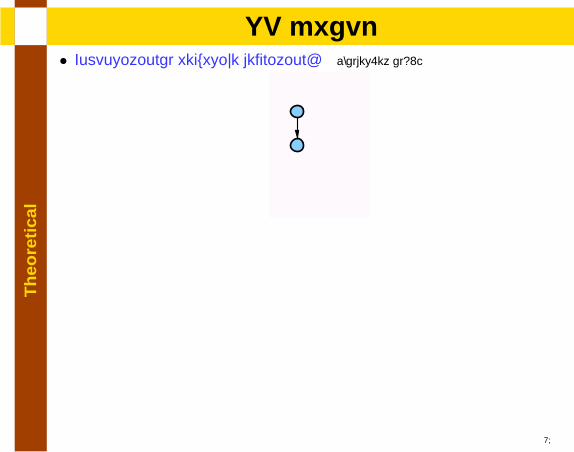
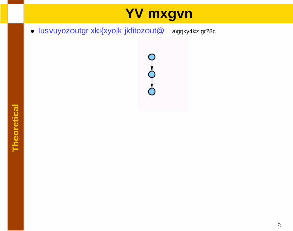
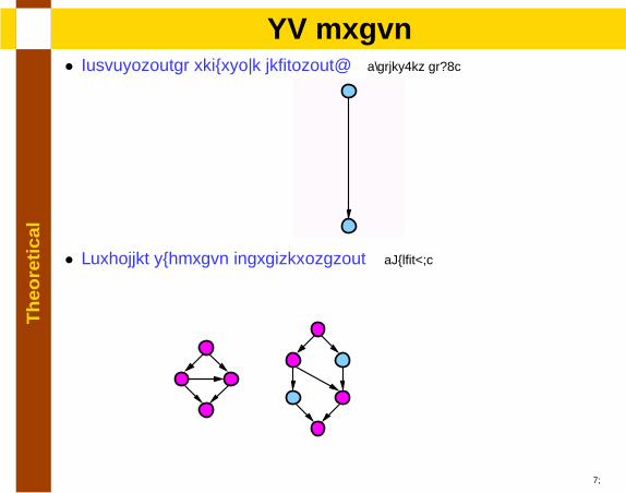
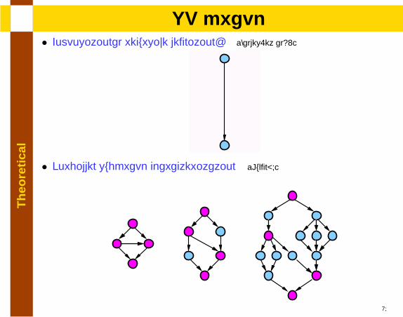
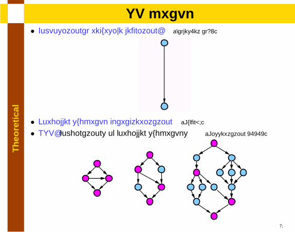
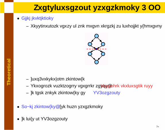
• Compositional recursive definition: [Valdes.et al92]
15
Th
eore
tica
lSP graph
• Compositional recursive definition: [Valdes.et al92]
15
Th
eore
tica
lSP graph
• Compositional recursive definition: [Valdes.et al92]
15
Th
eore
tica
lSP graph
• Compositional recursive definition: [Valdes.et al92]
15
Th
eore
tica
lSP graph
• Compositional recursive definition: [Valdes.et al92]
15

Th
eore
tica
lSP graph
• Compositional recursive definition: [Valdes.et al92]
15

Th
eore
tica
lSP graph
• Compositional recursive definition: [Valdes.et al92]
15

Th
eore
tica
lSP graph
• Compositional recursive definition: [Valdes.et al92]
15
Th
eore
tica
lSP graph
• Compositional recursive definition: [Valdes.et al92]
15

Th
eore
tica
lSP graph
• Compositional recursive definition: [Valdes.et al92]
15

Th
eore
tica
lSP graph
• Compositional recursive definition: [Valdes.et al92]
15
Th
eore
tica
lSP graph
• Compositional recursive definition: [Valdes.et al92]
15

Th
eore
tica
lSP graph
• Compositional recursive definition: [Valdes.et al92]
15
Th
eore
tica
lSP graph
• Compositional recursive definition: [Valdes.et al92]
15
Th
eore
tica
lSP graph
• Compositional recursive definition: [Valdes.et al92]
15

Th
eore
tica
lSP graph
• Compositional recursive definition: [Valdes.et al92]
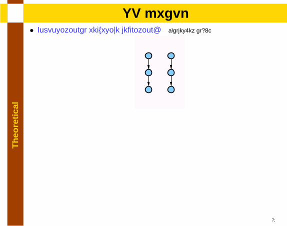
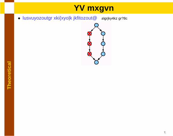
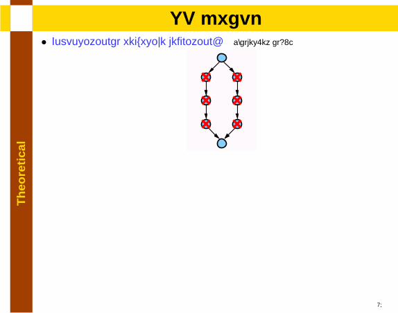
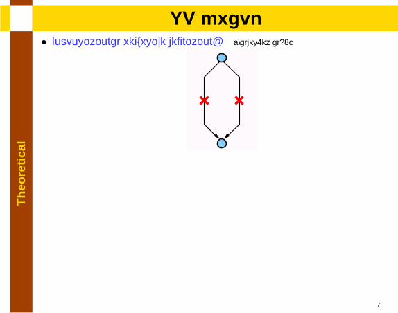
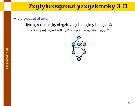
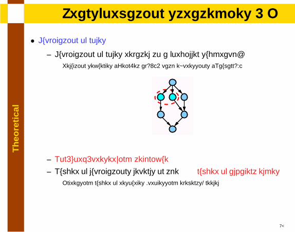
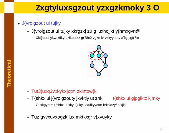
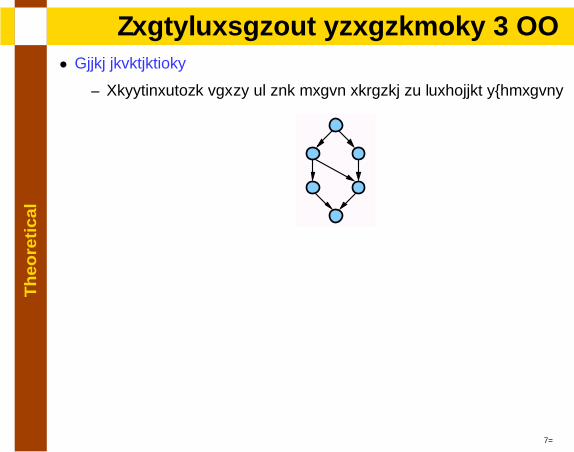
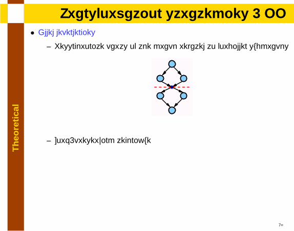
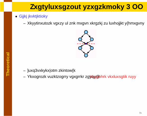
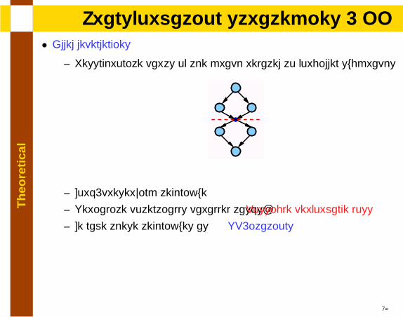
• Forbidden subgraph characterization [Duffin65]
15

Th
eore
tica
lSP graph
• Compositional recursive definition: [Valdes.et al92]
• Forbidden subgraph characterization [Duffin65]
15
Th
eore
tica
lSP graph
• Compositional recursive definition: [Valdes.et al92]
• Forbidden subgraph characterization [Duffin65]
15
Th
eore
tica
lSP graph
• Compositional recursive definition: [Valdes.et al92]
• Forbidden subgraph characterization [Duffin65]
15
Th
eore
tica
lSP graph
• Compositional recursive definition: [Valdes.et al92]
• Forbidden subgraph characterization [Duffin65]
• NSP: Combinations of forbidden subgraphs [Dissertation 3.3.3]
15
Th
eore
tica
lTransformation strategies - I
• Duplication of nodes
16
Th
eore
tica
lTransformation strategies - I
• Duplication of nodes
– Duplication of nodes related to a forbidden subgraph:Reduction sequences [Bein.et al92], path expressions [Naumann94]
16

Th
eore
tica
lTransformation strategies - I
• Duplication of nodes
– Duplication of nodes related to a forbidden subgraph:Reduction sequences [Bein.et al92], path expressions [Naumann94]
16
Th
eore
tica
lTransformation strategies - I
• Duplication of nodes
– Duplication of nodes related to a forbidden subgraph:Reduction sequences [Bein.et al92], path expressions [Naumann94]
16
Th
eore
tica
lTransformation strategies - I
• Duplication of nodes
– Duplication of nodes related to a forbidden subgraph:Reduction sequences [Bein.et al92], path expressions [Naumann94]
16
Th
eore
tica
lTransformation strategies - I
• Duplication of nodes
– Duplication of nodes related to a forbidden subgraph:Reduction sequences [Bein.et al92], path expressions [Naumann94]
16
Th
eore
tica
lTransformation strategies - I
• Duplication of nodes
– Duplication of nodes related to a forbidden subgraph:Reduction sequences [Bein.et al92], path expressions [Naumann94]
– Non-work-preserving technique
– Number of duplications depends on the number of adjacent edgesIncreasing number of resources (processing elements) needed
– Not appropriate for general purposes
16
Th
eore
tica
lTransformation strategies - II
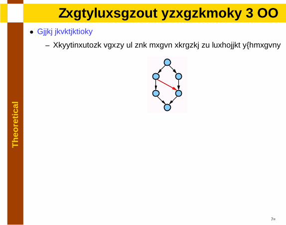
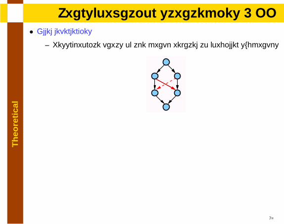
• Added dependencies
17

Th
eore
tica
lTransformation strategies - II
• Added dependencies
– Resynchronize parts of the graph related to forbidden subgraphs
17
Th
eore
tica
lTransformation strategies - II
• Added dependencies
– Resynchronize parts of the graph related to forbidden subgraphs
17
Th
eore
tica
lTransformation strategies - II
• Added dependencies
– Resynchronize parts of the graph related to forbidden subgraphs
17
Th
eore
tica
lTransformation strategies - II
• Added dependencies
– Resynchronize parts of the graph related to forbidden subgraphs
17

Th
eore
tica
lTransformation strategies - II
• Added dependencies
– Resynchronize parts of the graph related to forbidden subgraphs
17

Th
eore
tica
lTransformation strategies - II
• Added dependencies
– Resynchronize parts of the graph related to forbidden subgraphs
17
Th
eore
tica
lTransformation strategies - II
• Added dependencies
– Resynchronize parts of the graph related to forbidden subgraphs
17
Th
eore
tica
lTransformation strategies - II
• Added dependencies
– Resynchronize parts of the graph related to forbidden subgraphs
– Work-preserving technique
17
Th
eore
tica
lTransformation strategies - II
• Added dependencies
– Resynchronize parts of the graph related to forbidden subgraphs
– Work-preserving technique
– Serialize potentially parallel tasks: Possible performance loss
17
Th
eore
tica
lTransformation strategies - II
• Added dependencies
– Resynchronize parts of the graph related to forbidden subgraphs
– Work-preserving technique
– Serialize potentially parallel tasks: Possible performance loss
– We name these techniques as SP-izations
17
Th
eore
tica
lTransformation strategies - II
• Added dependencies
– Resynchronize parts of the graph related to forbidden subgraphs
– Work-preserving technique
– Serialize potentially parallel tasks: Possible performance loss
– We name these techniques as SP-izations
• Mixed techniques: Use both strategies
• We focus on SP-izations
17
Th
eore
tica
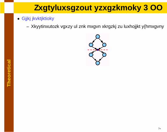
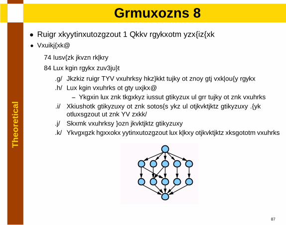
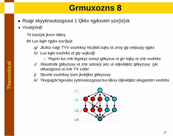
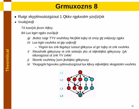
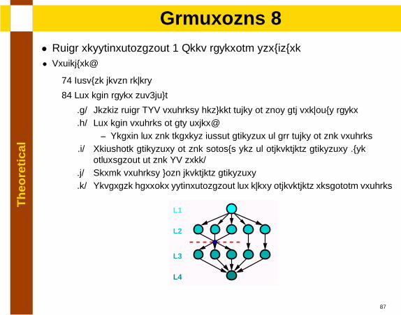
lLayering technique
• Well-known system [Malony.et al94] associated to the bulk-synchronousconcept
18
Th
eore
tica
lLayering technique
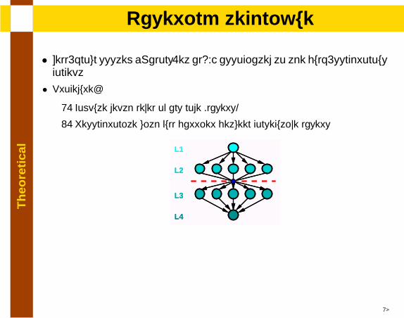
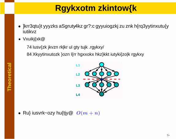
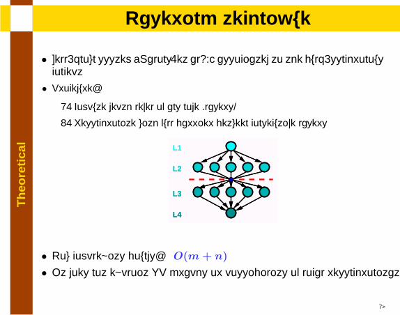
• Well-known system [Malony.et al94] associated to the bulk-synchronousconcept
• Procedure:
1. Compute depth level of any node (layers)
2. Resynchronize with full barrier between consecutive layers
18

Th
eore
tica
lLayering technique
• Well-known system [Malony.et al94] associated to the bulk-synchronousconcept
• Procedure:
1. Compute depth level of any node (layers)
2. Resynchronize with full barrier between consecutive layers
18
Th
eore
tica
lLayering technique
• Well-known system [Malony.et al94] associated to the bulk-synchronousconcept
• Procedure:
1. Compute depth level of any node (layers)
2. Resynchronize with full barrier between consecutive layers
L1
L2
L3
L4
18

Th
eore
tica
lLayering technique
• Well-known system [Malony.et al94] associated to the bulk-synchronousconcept
• Procedure:
1. Compute depth level of any node (layers)
2. Resynchronize with full barrier between consecutive layers
L1
L2
L3
L4
L1
L2
L3
L4
18
Th
eore
tica
lLayering technique
• Well-known system [Malony.et al94] associated to the bulk-synchronousconcept
• Procedure:
1. Compute depth level of any node (layers)
2. Resynchronize with full barrier between consecutive layers
L1
L2
L3
L4
L1
L2
L3
L4
L1
L2
L3
L4
18
Th
eore
tica
lLayering technique
• Well-known system [Malony.et al94] associated to the bulk-synchronousconcept
• Procedure:
1. Compute depth level of any node (layers)
2. Resynchronize with full barrier between consecutive layers
L1
L2
L3
L4
L1
L2
L3
L4
L1
L2
L3
L4
• Low complexity bounds: O(m+ n)
• It does not exploit SP graphs or possibility of local resynchronizations
18
Th
eore
tica
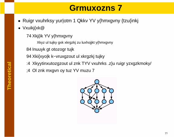
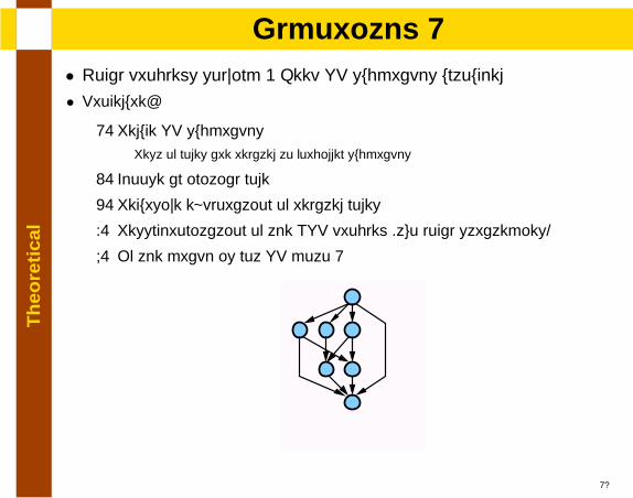
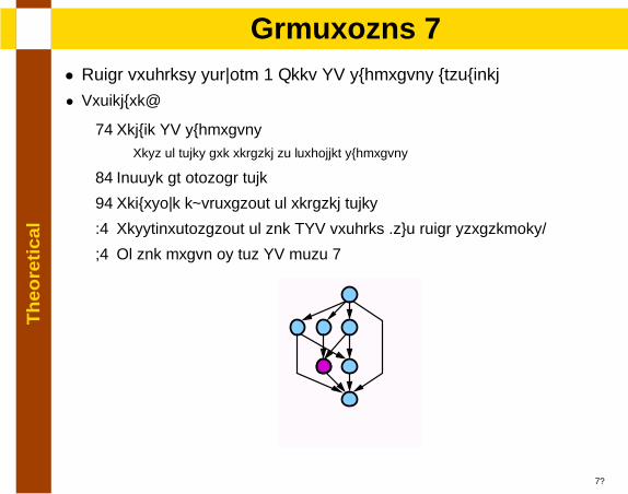
lAlgorithm 1
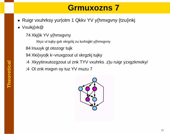
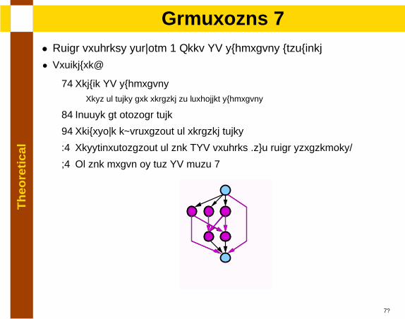
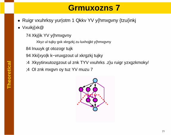
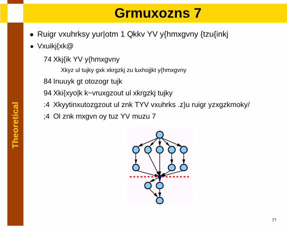
• Local problems solving + Keep SP subgraphs untouched
19
Th
eore
tica
lAlgorithm 1
• Local problems solving + Keep SP subgraphs untouched
• Procedure:
1. Reduce SP subgraphsRest of nodes are related to forbidden subgraphs
2. Choose an initial node
3. Recursive exploration of related nodes
4. Resynchronization of the NSP problem (two local strategies)
5. If the graph is not SP goto 1
19

Th
eore
tica
lAlgorithm 1: Properties
• A local combination is resynchronized in each iteration
20
Th
eore
tica
lAlgorithm 1: Properties
• A local combination is resynchronized in each iteration
• No global information stored: O(m× n)
20
Th
eore
tica
lAlgorithm 1: Properties
• A local combination is resynchronized in each iteration
• No global information stored: O(m× n)
• It does not keep the layering structure:Higher potential overhead even on well-balanced computations
20
Th
eore
tica
lAlgorithm 2
• Local resynchronization + Keep layering structure
21
Th
eore
tica
lAlgorithm 2
• Local resynchronization + Keep layering structure• Procedure:
1. Compute depth levels
2. For each layer top-down
(a) Detect local NSP problems between nodes in this and previous layer(b) For each problem in any order:
– Search for the nearest common ancestor of all nodes in the problem(c) Recombine ancestors in the minimum set of independent ancestors (use
information on the SP tree)(d) Merge problems with dependent ancestors(e) Separate barrier synchronization for every independent remaining problem
21

Th
eore
tica
lAlgorithm 2
• Local resynchronization + Keep layering structure• Procedure:
1. Compute depth levels
2. For each layer top-down
(a) Detect local NSP problems between nodes in this and previous layer(b) For each problem in any order:
– Search for the nearest common ancestor of all nodes in the problem(c) Recombine ancestors in the minimum set of independent ancestors (use
information on the SP tree)(d) Merge problems with dependent ancestors(e) Separate barrier synchronization for every independent remaining problem
L1
L2
L3
L4
21
Th
eore
tica
lAlgorithm 2
• Local resynchronization + Keep layering structure• Procedure:
1. Compute depth levels
2. For each layer top-down
(a) Detect local NSP problems between nodes in this and previous layer(b) For each problem in any order:
– Search for the nearest common ancestor of all nodes in the problem(c) Recombine ancestors in the minimum set of independent ancestors (use
information on the SP tree)(d) Merge problems with dependent ancestors(e) Separate barrier synchronization for every independent remaining problem
L1
L2
L3
L4
L1
L2
L3
L4
21

Th
eore
tica
lAlgorithm 2
• Local resynchronization + Keep layering structure• Procedure:
1. Compute depth levels
2. For each layer top-down
(a) Detect local NSP problems between nodes in this and previous layer(b) For each problem in any order:
– Search for the nearest common ancestor of all nodes in the problem(c) Recombine ancestors in the minimum set of independent ancestors (use
information on the SP tree)(d) Merge problems with dependent ancestors(e) Separate barrier synchronization for every independent remaining problem
L1
L2
L3
L4
L1
L2
L3
L4
L1
L2
L3
L4
21
Th
eore
tica
lAlgorithm 2: Properties
• Considers global information stored in the SP tree-reduction
22
Th
eore
tica
lAlgorithm 2: Properties
• Considers global information stored in the SP tree-reduction
• Tight time complexity bounds: O(m+ n logn)
Higher complexity than the layering technique
22
Th
eore
tica
lAlgorithm 2: Properties
• Considers global information stored in the SP tree-reduction
• Tight time complexity bounds: O(m+ n logn)
Higher complexity than the layering technique
• Similar results as layering for regular NSP structuresBut better results for more irregular, or closer to SP form graphs
22

Th
eore
tica
lImpact indicator
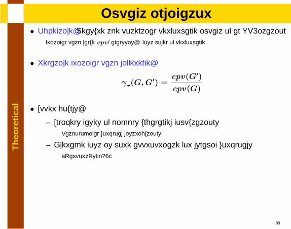
• Objective: Measure the potential performance impact of an SP-izationCritical path value (cpv) analysis: Cost model of performance
23
Th
eore
tica
lImpact indicator
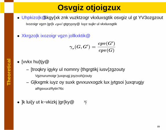
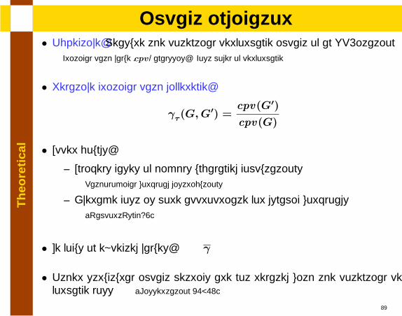
• Objective: Measure the potential performance impact of an SP-izationCritical path value (cpv) analysis: Cost model of performance
• Relative critical path difference:
γτ (G,G′) =
cpv(G′)
cpv(G)
23
Th
eore
tica
lImpact indicator
• Objective: Measure the potential performance impact of an SP-izationCritical path value (cpv) analysis: Cost model of performance
• Relative critical path difference:
γτ (G,G′) =
cpv(G′)
cpv(G)
• Upper bounds:
– Unlikely cases of highly unbalanced computationsPathological workload distributions
– Average cost is more appropriate for dynamic workloads[LamportLynch90]
• We focus on expected values: γ
• Other structural impact metrics are not related with the potential per-formance loss [Dissertation 3.6.2]
23
Th
eore
tica
lSP vs. NSP cpv analysis
• Absence of real workload information: Stochastic workloads
24
Th
eore
tica
lSP vs. NSP cpv analysis
• Absence of real workload information: Stochastic workloadsNodes workload are i.i.d. (independent identically distributed) random variables
24
Th
eore
tica
lSP vs. NSP cpv analysis
• Absence of real workload information: Stochastic workloadsNodes workload are i.i.d. (independent identically distributed) random variables
• Stochastic SP cpv analysis:
– Series composition: Addition of i.i.d. random variables
– Parallel composition: Order statistics [Gumbel62]
• Stochastic NSP cpv analysis: Prevented by its inherent complexity
• Approximations for simple regular NSP structures [Vaca99]
– Simple analytical formulae for γ
– Predicts experimental behavior asymptotically (Error < 25%)
– Topology-dependent results
• Further experimental study is neededto predict the loss of performance in a generic case
24
Exp
erim
enta
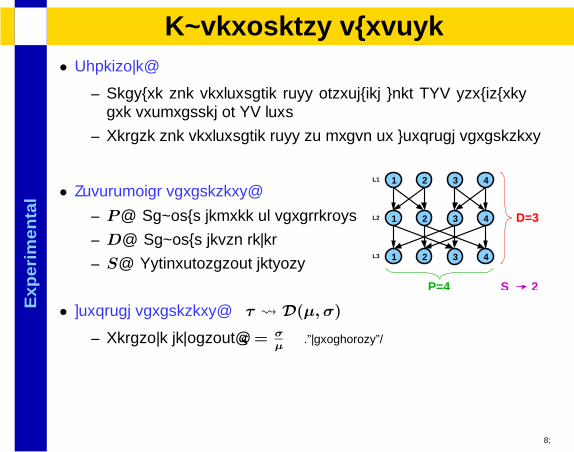
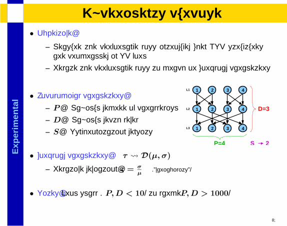
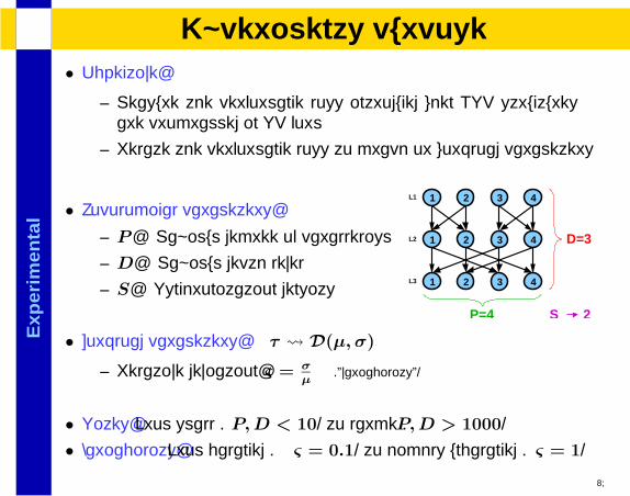
lExperiments purpose
• Objective:
– Measure the performance loss introduced when NSP structuresare programmed in SP form
– Relate the performance loss to graph or workload parameters
25
Exp
erim
enta
lExperiments purpose
• Objective:
– Measure the performance loss introduced when NSP structuresare programmed in SP form
– Relate the performance loss to graph or workload parameters
• Topological parameters:
– P : Maximum degree of parallelism
– D: Maximum depth level
– S: Synchronization density 1 2 43
1 2 43
1 2 43
S 2
D=3
P=4
L1
L2
L3
• Workload parameters: τ D(µ, σ)
– Relative deviation: ς = σµ
(”variability”)
• Sizes: From small (P,D < 10) to large (P,D > 1000)
• Variability: From balanced (ς = 0.1) to highly unbalanced (ς = 1)
25
Exp
erim
enta
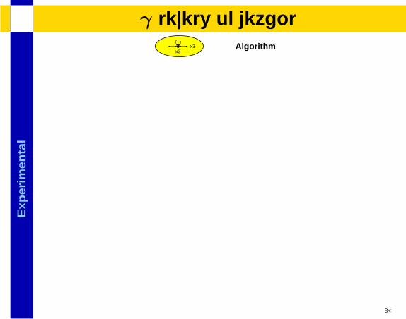
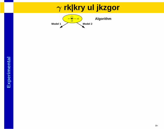
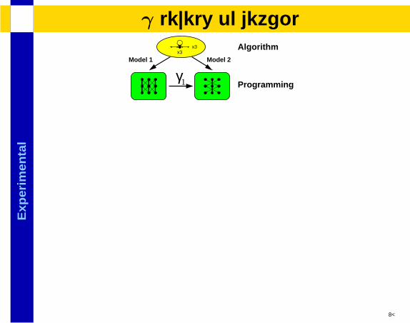
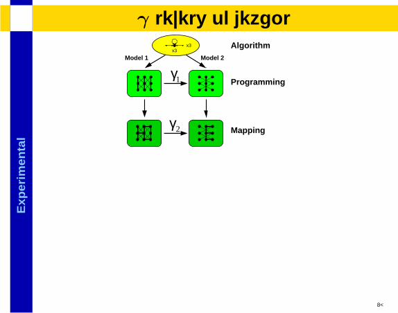
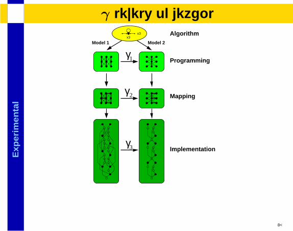
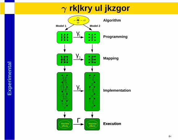
lγ levels of detail
x3x3 Algorithm
26
Exp
erim
enta
lγ levels of detail
x3x3 Algorithm
Model 1 Model 2
26
Exp
erim
enta
lγ levels of detail
x3x3 Algorithm
Model 1 Model 2
γ1 Programming
26
Exp
erim
enta
lγ levels of detail
x3x3 Algorithm
Model 1 Model 2
γ1 Programming
γ2 Mapping
26
Exp
erim
enta
lγ levels of detail
x3x3 Algorithm
Model 1 Model 2
γ1 Programming
γ2 Mapping
3γImplementation
26

Exp
erim
enta
lγ levels of detail
x3x3 Algorithm
Model 1 Model 2
γ1 Programming
γ2 Mapping
3γImplementation
ΓExecutionMachine
effectsMachineeffects
26
Exp
erim
enta
lγ levels of detail
x3x3 Algorithm
Model 1 Model 2
γ1 Programming
γ2 Mapping
3γImplementation
ΓExecutionMachine
effectsMachineeffects
ΓExecutionMachine
effectsMachineeffects
26
Exp
erim
enta
lExperiments design - I
• Exhaustive testing of the graph space is impossible
27
Exp
erim
enta
lExperiments design - I
• Exhaustive testing of the graph space is impossible
• Approaches:
27
Exp
erim
enta
lExperiments design - I
• Exhaustive testing of the graph space is impossible
• Approaches:
Experiments
27

Exp
erim
enta
lExperiments design - I
• Exhaustive testing of the graph space is impossible
• Approaches:
Experiments
Synthetic graphs
Random sample graphs
Meshes
27

Exp
erim
enta
lExperiments design - I
• Exhaustive testing of the graph space is impossible
• Approaches:
Experiments
Synthetic graphs
Random sample graphs
Meshes
Real applications
Static applications
Dynamic applications
27
Exp
erim
enta
lExperiments design - II
Synthetic graphs
• Random sample of the graph space: General idea of trends
28
Exp
erim
enta
lExperiments design - II
Synthetic graphs
• Random sample of the graph space: General idea of trends
– Random graphs generation technique [Almeida92]
– Parameters: Size, S, ς
28
Exp
erim
enta
lExperiments design - II
Synthetic graphs
• Random sample of the graph space: General idea of trends
– Random graphs generation technique [Almeida92]
– Parameters: Size, S, ς
• Meshes: Regular topologies of i layers with j nodes each
28
Exp
erim
enta
lExperiments design - II
Synthetic graphs
• Random sample of the graph space: General idea of trends
– Random graphs generation technique [Almeida92]
– Parameters: Size, S, ς
• Meshes: Regular topologies of i layers with j nodes each
– Regular or random synchronization between consecutive layers[TobitaKasahara99]
– Parameters: P,D, S, ς
• Workload: 25 draws for each topology and ς value
28
Exp
erim
enta
lExperiments design - III
Real static applications
• Easy graph modeling at any level of detail
29

Exp
erim
enta
lExperiments design - III
Real static applications
• Easy graph modeling at any level of detail
• Typically highly regular: Results expected to be similar than meshes
29
Exp
erim
enta
lExperiments design - III
Real static applications
• Easy graph modeling at any level of detail
• Typically highly regular: Results expected to be similar than meshes
• Parameters: P,D
29
Exp
erim
enta
lExperiments design - III
Real static applications
• Easy graph modeling at any level of detail
• Typically highly regular: Results expected to be similar than meshes
• Parameters: P,D
• Macro-pipeline, Cellular Automata, FFT, LU reduction
29
Exp
erim
enta
lExperiments design - III
Real static applications
• Easy graph modeling at any level of detail
• Typically highly regular: Results expected to be similar than meshes
• Parameters: P,D
• Macro-pipeline, Cellular Automata, FFT, LU reduction
• Framework (γ,Γ):
– Programming/mapping levels: Synthetic workloads
– Implementation level: Communication costs considered
– Execution level: MPI implementations (SP version with barriers)[Dissertation 4.2.1]
• Execution level: Three architectures
– CC-NUMA (Origin2000)
– Message-passing with low latency (CrayT3E)
– Distributed memory with high latency (Beowulf)
29

Exp
erim
enta
lExperiments design - IV
Real dynamic applications
• Two cases:
1. Structure can be reconstructed from input data structure
2. Structure can be obtained only by tracing in run-time
30
Exp
erim
enta
lExperiments design - IV
Real dynamic applications
• Two cases:
1. Structure can be reconstructed from input data structure
2. Structure can be obtained only by tracing in run-time
• Typically more irregular than static applications
• One example application of each type
• Six real input data examples for each application
30
Exp
erim
enta
lExperiments design - V
Iterative PDE solver
31
Exp
erim
enta
lExperiments design - V
Iterative PDE solver
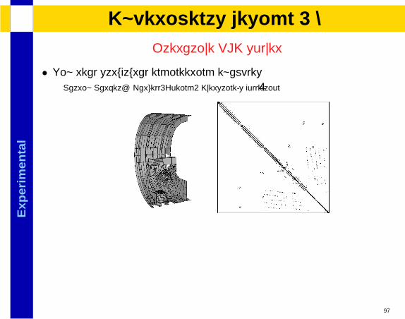
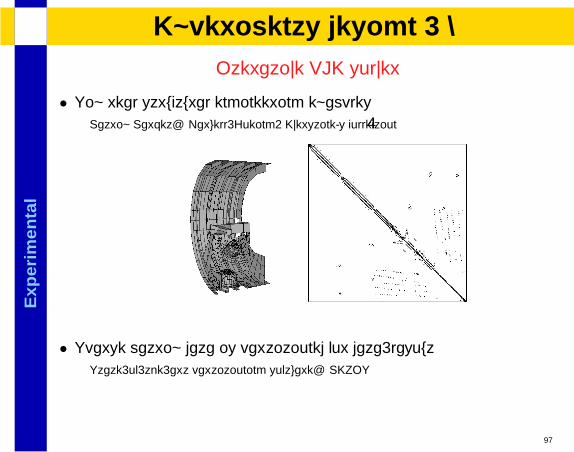
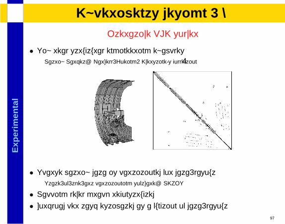
• Six real structural engineering examplesMatrix Market: Harwell-Boeing, Everstine’s collection.
31
Exp
erim
enta
lExperiments design - V
Iterative PDE solver
• Six real structural engineering examplesMatrix Market: Harwell-Boeing, Everstine’s collection.
• Sparse matrix data is partitioned for data-layoutState-of-the-art partitioning software: METIS
31
Exp
erim
enta
lExperiments design - V
Iterative PDE solver
• Six real structural engineering examplesMatrix Market: Harwell-Boeing, Everstine’s collection.
• Sparse matrix data is partitioned for data-layoutState-of-the-art partitioning software: METIS
• Mapping level graph reconstructed
• Workload per task estimated as a function of data-layout31
Exp
erim
enta
lExperiments design - VI
Domain decomposition and sparse matrix factorization
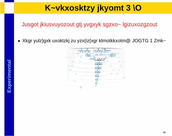
• Real software oriented to structural engineering: DIANA + Tgex
330
2400
2000 14001600 600400 400400
6
6384
13230
4536 4455 12151080 810
881
1124
3760
2896 9841488 1468474
784 294196 196196
363
9
4
4984
36 3636
4
4408
297
2
13
1616
293
2
7
8533
7475 174845541104276
16
1
4540535014001674 852
1125
8550 45003150900 900
0
970
330
0
1400 1600 600400 400400
254
2
30
13
2280
866472205054 5776 21661444 14441444
0
5662
5453 2584266
848
576
47
1202
7778
28802016 2304 864576 576576
1016
168
19
384256 256256
9
13572
5684 66126496 5684928 1160580
0
4155
3025
1720
7
5
5
5
14 53
33
1 1
1
1
1
1
71 372677
17 20
75
55 574733 38 149 99
30
21
24 9
6
66
47524300 3608612
60151740 4260 1620 1080300
7244 8756 3312 22082734
145486622 16272 45182756 39723108
11504 51455160 34304284
3524
36284472
39323590
3668
46903283938
14482 13752 37204840 33484360
32
Exp
erim
enta
lExperiments design - VI
Domain decomposition and sparse matrix factorization
• Real software oriented to structural engineering: DIANA + Tgex
330
2400
2000 14001600 600400 400400
6
6384
13230
4536 4455 12151080 810
881
1124
3760
2896 9841488 1468474
784 294196 196196
363
9
4
4984
36 3636
4
4408
297
2
13
1616
293
2
7
8533
7475 174845541104276
16
1
4540535014001674 852
1125
8550 45003150900 900
0
970
330
0
1400 1600 600400 400400
254
2
30
13
2280
866472205054 5776 21661444 14441444
0
5662
5453 2584266
848
576
47
1202
7778
28802016 2304 864576 576576
1016
168
19
384256 256256
9
13572
5684 66126496 5684928 1160580
0
4155
3025
1720
7
5
5
5
14 53
33
1 1
1
1
1
1
71 372677
17 20
75
55 574733 38 149 99
30
21
24 9
6
66
47524300 3608612
60151740 4260 1620 1080300
7244 8756 3312 22082734
145486622 16272 45182756 39723108
11504 51455160 34304284
3524
36284472
39323590
3668
46903283938
14482 13752 37204840 33484360
• We use six example mapping level graphs reconstructed from tracinginformation obtained in a previous work [Lin94,96]
• Real execution workloads provided
32
Exp
erim
enta
lResults: Workload
1
1.2
1.4
1.6
1.8
2
0 128 256 384 512 640 768 896 1024
γ�
# nodes
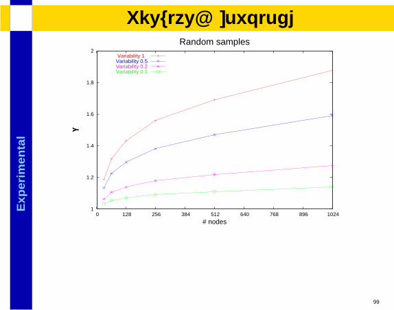
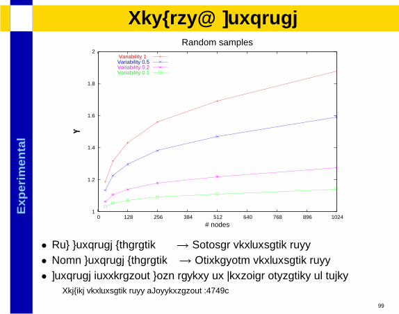
Random samplesVariability 1 Variability 0.5Variability 0.2Variability 0.1
33
Exp
erim
enta
lResults: Workload
1
1.2
1.4
1.6
1.8
2
0 128 256 384 512 640 768 896 1024
γ�
# nodes
Random samplesVariability 1 Variability 0.5Variability 0.2Variability 0.1
• Low workload unbalance→ Minimal performance loss• High workload unbalance→ Increasing performance loss
33
Exp
erim
enta
lResults: Workload
1
1.2
1.4
1.6
1.8
2
0 128 256 384 512 640 768 896 1024
γ�
# nodes
Random samplesVariability 1 Variability 0.5Variability 0.2Variability 0.1
• Low workload unbalance→ Minimal performance loss• High workload unbalance→ Increasing performance loss• Workload correlation with layers or vertical instances of nodes
Reduced performance loss [Dissertation 4.1.3]
33
Exp
erim
enta
lResults: Graph size parameters P,D
34
Exp
erim
enta
lResults: Graph size parameters P,D
1
1.2
1.4
1.6
1.8
2
0 200 400 600 800 1000
γ�
P
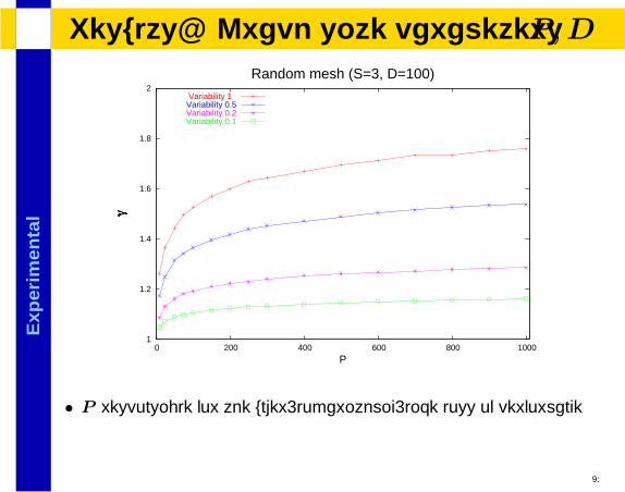
Random mesh (S=3, D=100)Variability 1 Variability 0.5Variability 0.2Variability 0.1
• P responsible for the under-logarithmic-like loss of performance
34
Exp
erim
enta
lResults: Graph size parameters P,D
1
1.2
1.4
1.6
1.8
2
0 200 400 600 800 1000
γ�
D
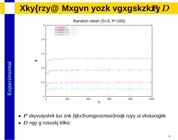
Random mesh (S=3, P=100)Variability 1 Variability 0.5Variability 0.2Variability 0.1
• P responsible for the under-logarithmic-like loss of performance• D has a limited effect
34

Exp
erim
enta
lResults: Graph size parameters P,D
1
1.2
1.4
1.6
1.8
2
0 200 400 600 800 1000
γ�
D
Random mesh (S=3, P=100)Variability 1 Variability 0.5Variability 0.2Variability 0.1
• P responsible for the under-logarithmic-like loss of performance• D has a limited effect
Pathological effects characterization and metric [Dissertation 4.1.3]
34

Exp
erim
enta
lResults: Graph parameter S
1
1.2
1.4
1.6
1.8
2
1 10 100
γ�
S
Random sample: 256 nodesVariability 1 Variability 0.1
• S increase has opposite effect to P
35

Exp
erim
enta
lResults: Graph parameter S
1
1.2
1.4
1.6
1.8
2
1 10 100
γ�
S
Random sample: 256 nodesVariability 1 Variability 0.1
• S increase has opposite effect to P
• S < 2 implies sparse graphs containing SP series subgraphs
35
Exp
erim
enta
lResults: Graph parameter S
1
1.2
1.4
1.6
1.8
2
1 10 100
γ�
S
Random sample: 256 nodesVariability 1 Variability 0.1
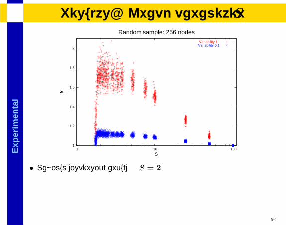
• Maximum dispersion around S = 2
36

Exp
erim
enta
lResults: Graph parameter S
1
1.2
1.4
1.6
1.8
2
1 10 100
γ�
S
Random sample: 256 nodesVariability 1 Variability 0.1
• Maximum dispersion around S = 2
• Asymptotic predictions:
γ ≈µ+ σ
√log(P )
µ+ σ√
log(S)36
Exp
erim
enta
lResults: Execution level Γ
37
Exp
erim
enta
lResults: Execution level Γ
0.96
0.98
1
1.02
1.04
1.06
1.08
1.1
2 4 6 8 10 12 14 16
Γ�
# Procs.
Beowulf - GammaMacro-Pipeline
Cellular AutomataLU reduction
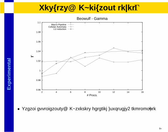
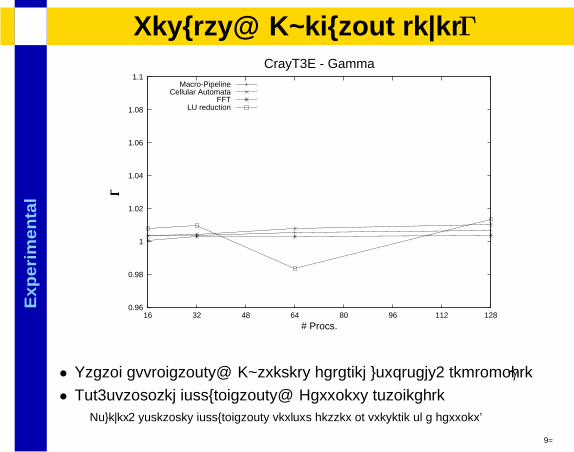
• Static applications: Extremely balanced workloads, negligible γ
37

Exp
erim
enta
lResults: Execution level Γ
0.96
0.98
1
1.02
1.04
1.06
1.08
1.1
2 4 6 8 10 12 14 16
Γ�
# Procs.
Beowulf - GammaMacro-Pipeline
Cellular AutomataLU reduction
• Static applications: Extremely balanced workloads, negligible γ
• Non-optimized communications: Barriers noticeable
37
Exp
erim
enta
lResults: Execution level Γ
0.96
0.98
1
1.02
1.04
1.06
1.08
1.1
16 32 48 64 80 96 112 128
Γ�
# Procs.
CrayT3E - GammaMacro-Pipeline
Cellular AutomataFFT
LU reduction
• Static applications: Extremely balanced workloads, negligible γ
• Non-optimized communications: Barriers noticeableHowever, sometimes communications perform better in presence of a barrier!
37
Exp
erim
enta
lResults: Dynamic applications - I
Sparse iterative solvers
• METIS partitioning produces very well workload and synchronizationbalance
38
Exp
erim
enta
lResults: Dynamic applications - I
Sparse iterative solvers
• METIS partitioning produces very well workload and synchronizationbalance
38

Exp
erim
enta
lResults: Dynamic applications - I
Sparse iterative solvers
• METIS partitioning produces very well workload and synchronizationbalance
150
159
157
153
152
Workload
38

Exp
erim
enta
lResults: Dynamic applications - I
Sparse iterative solvers
• METIS partitioning produces very well workload and synchronizationbalance
150
159
157
153
152
Workload
• Negligible loss of performance: Expected for any good load-balancingtechnique
38

Exp
erim
enta
lResults: Dynamic applications - II
Domain decomposition and sparse matrix factorization
39
Exp
erim
enta
lResults: Dynamic applications - II
Domain decomposition and sparse matrix factorization
• Bad statistical workload parameters: ς � 1 in most cases
39
Exp
erim
enta
lResults: Dynamic applications - II
Domain decomposition and sparse matrix factorization
• Bad statistical workload parameters: ς � 1 in most cases
• Experiments with synthetic workloads show lower γ than expected
• Real workload even lower:
# nodes ς Γ59 2.1 1.000
113 3.0 1.006213 1.4 1.074528 2.0 1.199773 7.1 1.009
2015 2.6 1.103
• Domain decomposition data-layout produces workloadand topology regularities
39
Co
ncl
usi
onSummary
• Parallel programming field: Lack of a common development direction
40
Co
ncl
usi
onSummary
• Parallel programming field: Lack of a common development direction
• We have proposed a new classification system for PPMs, based on SA
The adequacy of a model in terms of expressive power, software de-velopment methodologies and analyzability characteristics, is relatedto its SA class
• The SP-restriction is a critical decision for a PPM adequacy
SA: Key for the expressive power vs. analyzability trade-off
• The expressive power restriction associated with SP PPMs has beeninvestigated in-depth both theoretically and empirically
40
Co
ncl
usi
on
Methodology
• Methodology: Three-way approach
– Conceptual: Models and applications review, SA classification.Qualitative study
41
Co
ncl
usi
on
Methodology
• Methodology: Three-way approach
– Conceptual: Models and applications review, SA classification.Qualitative study
– Theoretical: SP, NSP graph characterizationand algorithmic transformation techniques
41

Co
ncl
usi
on
Methodology
• Methodology: Three-way approach
– Conceptual: Models and applications review, SA classification.Qualitative study
– Theoretical: SP, NSP graph characterizationand algorithmic transformation techniques
– Experimental: Empirical analysis framework for the potentialnegative performance impact of SP programming at differentlevels of detail, including propagation to execution level
41

Co
ncl
usi
on
Results• At the design or programming level (γ):
Correlation between the SP potential loss of parallelism with simpleapplication parameters:
– P has an under-logarithmic-like effect on γ
– S has a positive inverse effect
– Variability (ς) has the major impact on γ
42
Co
ncl
usi
on
Results• At the design or programming level (γ):
Correlation between the SP potential loss of parallelism with simpleapplication parameters:
– P has an under-logarithmic-like effect on γ
– S has a positive inverse effect
– Variability (ς) has the major impact on γ
• At execution level (Γ):In our experiments with real applications Γ is bounded to tens of per-centsIt almost does not scale with the problem size!
• SP performance degradation is mainly associated to poorly balancedand unstructured computations
• SP SA is a promising design concept for portable, efficient, easy-to-use and general-purpose PPMs
42
Co
ncl
usi
on
On-going and future research
• Further experiments with more irregular applications
43

Co
ncl
usi
on
On-going and future research
• Further experiments with more irregular applications
• New NSP to SP transformations:
– Based on both strategies
– Using information of estimated workload
43
Co
ncl
usi
on
On-going and future research
• Further experiments with more irregular applications
• New NSP to SP transformations:
– Based on both strategies
– Using information of estimated workload
• Real SP programming framework development:Automatic mapping and scheduling guided by performance cost analysis
43
Co
ncl
usi
on
Main contributions
• CPC 2003, Tenth International Workshop on Compilers for Parallel Computers, Amsterdam,The Netherlands
• VecPar 2002, 5th International Meeting, High Performance Computing for Computational Sci-ence, Porto, Portugal (Best Student Paper Award)
• CPC 2001, Ninth International Workshop on Compilers for Parallel Computers, Edinburgh,Scotland
• VecPar 2000, 4th International Meeting on Vector and Parallel Processing, Porto, Portugal
• CPC 2000, Eigth International Workshop on Compilers for Parallel Computers, Aussois, France
• Parallel Computing ParCo’99 Delft, The Netherlands
• Euro-PDS’97, IASTED International Conference, Parallel and Distributed Systems, Barcelona
• ASCI’97, Proceedings of the third annual conference of the Advanced School for Computingand Imaging, Heijen
44

Questions?
Powered by: LATEX, Xfig, Gnuplot, PPower4, Acrobat Reader
45