synchronisation effects on the behavioural performance and information...
TRANSCRIPT

Noname manuscript No.(will be inserted by the editor)
Synchronisation effects on the behavioural performance and informationdynamics of a simulated minimally cognitive robotic agent
Renan C. Moioli, Patricia A. Vargas, Phil Husbands
Abstract Oscillatory activity is ubiquitous in nervous sys-tems, with solid evidence that synchronisation mechanismsunderpin cognitive processes. Nevertheless, its informationalcontent and relationship with behaviour are still to be fullyunderstood. Additionally, cognitive systems cannot be prop-erly appreciated without taking into account brain - body- environment interactions. In this paper, we developed amodel based on the Kuramoto Model of coupled phase os-cillators to explore the role of neural synchronisation in theperformance of a simulated robotic agent in two differentminimally cognitive tasks. We show that there is a statisti-cally significant difference in performance and evolvabilitydepending on the synchronisation regime of the network. Inboth tasks, a combination of information flow and dynami-cal analyses show that networks with a definite, but not toostrong, propensity for synchronisation are more able to re-configure, to organise themselves functionally and to adaptto different behavioural conditions. The results highlight theasymmetry of information flow and its behavioural corre-spondence. Importantly it also shows that neural synchroni-sation dynamics, when suitably flexible and reconfigurable,can generate minimally cognitive embodied behaviour.
Keywords Synchronisation· Evolutionary Robotics·Oscillatory networks· Transfer Entropy· Kuramoto Model
1 Introduction
Oscillatory neural activity is closely related to cognitive pro-cesses and behaviour (Engel et al., 2001; Buzsaki, 2006).
Renan C. Moioli and Phil Husbands are with the Centre for Compu-tational Neuroscience and Robotics (CCNR), Department of Informat-ics, University of Sussex, Falmer, Brighton, BN1 9QH, United King-dom, (email:{r.moioli, p.husbands}@sussex.ac.uk). Patricia A. Vargasis with the School of Mathematical and Computer Science, Heriot-WattUniversity, Edinburgh, Scotland, EH14 4AS, United Kingdom, (email:[email protected])
More specifically, it has been claimed that the flexible syn-chronisation of firing neurons is a fundamental brain mecha-nism (von der Malsburg, 1981; Singer, 1993, 1999; Womels-dorf et al., 2007). Synchronisation may mediate the interac-tions between neurons and be an active mechanism of large-scale integration of neuronal assemblies, impacting on mo-tor control and cognitive performance (Hatsopoulos et al.,1998; Varela et al., 2001; Jackson et al., 2003). Moreover,a range of pathological states are related to abnormal neu-ronal synchronisation regimes (Glass, 2001; Brown, 2003;Arthuis et al., 2009).
Whereas increasingly sophisticated computational andimaging techniques help us to observe and record from dif-ferent physiological aspects of the nervous system, a greatpart of the challenge lies in the comprehension of this ava-lanche of data and its relationship with behaviour (Chialvo,2010). In addition, the brain presents spontaneous electro-chemical activity that is constantly shaped by the body’sconstraints and time-varying environmental stimuli (Katz,1999). The brain, therefore, not only processes informationbut also produces it, and cognitive phenomena are a prod-uct of brain-body-environment interactions (Stewart et al.,2010). Situated artificial agents, in this sense, provide anap-propriate experimental scenario to study the principles ofin-telligent behaviour (Boden, 2006).
There is a rich literature exploring the relationship be-tween neural synchronisation and complex motor controlin embodied (robotic) rhythmical behaviours (Taga, 1994;Ijspeert et al., 2005; Pitti et al., 2009), where synchroni-sation appears as a more intuitive underlying mechanism;however, to date there has been very little research on thewider issues of neuronal synchronisation in the generationof embodied cognitive behaviours. Therefore, using conceptsfrom Evolutionary Robotics (Harvey et al., 2005; Floreanoet al., 2008; Floreano & Mattiussi, 2008; Floreano & Keller,2010), we explore the role of synchronisation in the perfor-mance of a simulated robotic agent during the execution of

2 Renan C. Moioli, Patricia A. Vargas, Phil Husbands
two different minimally cognitive tasks: the first, a categor-ical perception task (Beer, 2003; Izquierdo, 2008; Dale &Husbands, 2010), in which the robot has to discriminate be-tween moving circles and squares; the second, an orientationtask, where the robotic agent has to approach moving cir-cles with both normal and inverted vision, adapting to bothconditions. These tasks were chosen for being currently re-garded as benchmarks in the evolutionary robotics and adap-tive behaviour communities, with categorical perception un-derpinning cognitive systems (Harnad, 1987).
The work reported here is intended to shed some lighton the role of neural synchronisation in simple embodiedcognitive behaviours. More specifically it aims to1) testwhether different degrees of coupling in the agent’s oscilla-tory neural network, which will encourage more or less syn-chrony in the network dynamics, have an effect on the per-formance of the agent and2) determine if there are circum-stances in which more (or less) synchrony is better suitedto the generation of adaptive behaviour in the context of thetasks studied.
The neuronal model employed is based on the KuramotoModel of coupled phase oscillators (Kuramoto, 1984), whichhas been extensively studied in the Statistical Physics liter-ature, with recent applications in a biological context dueto its relatively simple and abstract mathematical formula-tion yet complex activity that can be exploited to clarifyfundamental mechanisms of neuro-oscillatory phenomenawithout making too many a priori assumptions (Ermentrout& Kleinfeld, 2001; Cumin & Unsworth, 2007; Kitzbichleret al., 2009; Breakspear et al., 2010). The model explicitlycaptures the phase dynamics of units that alone have spon-taneous oscillatory activity and once connected can gener-ate emergent rhythmic patterns. Its synchronisation regimecan be adjusted by one parameter (Strogatz, 2000), suitingour study, whilst also avoiding any problems in obtainingphase information (an issue in other models which considerfrequency and amplitude dynamics (Pikovsky et al., 2001)).Phase relationships contain a great deal of information onthe temporal structure of neural signals, are associated withcognition and relate to memory formation and retrieval (Li& Hopfield, 1989; Izhikevich, 1999; Varela et al., 2001; Kun-yosi & Monteiro, 2009). Furthermore, it has been shown thatfiring and bursting neurons can be modelled as oscillators(Murray, 1989). Hence the Kuramoto model is highly rel-evant, at a certain level of abstraction, to modelling neuralmechanisms underlying adaptive and cognitive behaviours.
Analysis of results is centred on how the information dy-namics between the nodes of the network, the agent’s bodyand the environment vary depending on the current synchro-nisation status of the system and how this is reflected in thebehaviour being displayed. Information Theory provides aframework for quantifying and emphasizing the non-linearrelationships between variables of the system, hence its suit-
ability in Biology and Robotics studies (Rieke et al., 1997;Rolls & Treves, 1998; Lungarella & Sporns, 2006). In thiscontext, agent-environment systems pose extra challengesin devising and interpreting a sensible measurement of in-formation flow, for they normally have noisy and limiteddata samples, asymmetrical relationships among elementsof the system and temporal variance (i.e. sensory and mo-tor patterns may vary over time). Transfer Entropy, in thisscenario, is suggested as a suitable and robust informationtheoretic tool (Lungarella et al., 2007b,a), and has also beenapplied to investigate real neural assemblies and other neu-roscience problems (Borst & Theunissen, 1999; Gourevitch& Eggermont, 2007; Buehlmann & Deco, 2010; McDonnellet al., 2011; Vicente et al., 2011); it will, thus, be used in ouranalysis.
The paper is organised as follows: the next section pres-ents some theoretical background to the main concepts ex-plored in this work: oscillators and synchronisation, focus-ing on the Kuramoto Model, evolutionary robotics (ER) andthe two minimally cognitive tasks studied, and InformationTheory in an agent-environment context, describing Trans-fer Entropy. We then present the methods adopted to developthe experiments and analysis, covering the ER framework,the details of the active categorical perception and orienta-tion under normal and inverted vision tasks, a descriptionof the genetic algorithm used to optimize the parameters ofthe system, and concluding with details of the time-seriesanalysis using Transfer Entropy. Following this, we presentthe results, which show a difference in performance and be-haviour depending on the synchronisation regime of the net-work, relating the observed sensorimotor strategies with thedynamics and the information flow of the system. The papercloses with a discussion on the results obtained and futurework proposals.
2 Theoretical Background
2.1 Oscillators, Synchronisation and The Kuramoto Model
In a study pioneered by Winfree (Winfree, 1980), the dy-namics of a population of interacting limit-cycle oscillatorshave been approximated by a population of interacting phaseoscillators, leading to a mean-field approximation model ex-tensively explored by Kuramoto (Kuramoto, 1984). In hisapproach, the phase of each oscillator is determined by itsnatural frequency (drawn from some distribution) modulatedaccording to a function that represents its sensitivity to thephase in every other node (see Equation 1)
dθidt
= ωi +N
∑
j=1
Γij(θj − θi), i = 1, . . . , N. (1)

Title Suppressed Due to Excessive Length 3
where:θi is the phase of theith oscillator,ωi is the naturalfrequency of theith oscillator,Γij represents the interactionbetween nodes andN is the total number of oscillators.
If one considers the interaction function to be periodic,i.e. Γij(x + 2π) = Γij(x), it can then be expanded into aFourier series. Considering only the first term of this series,and specifying that the network is symmetrically coupled,the previous model reduces to Equation 2, which is knownas the Kuramoto Model:
dθidt
= ωi +K
N
N∑
j=1
sin(θj − θi), i = 1, . . . , N. (2)
Basically, if the frequency of all possible pairs of nodesi and j (i, j = 1, 2...n) are equal, i.e.dθi − dθj = 0 orθi − θj = constant, the model is said to be globally syn-chronised. It is possible to calculate a synchronisation index,which gives a good idea of how synchronised the set of os-cillators are (Kuramoto, 1984). Consider Equation 3, wherer is the synchronisation index (1 meaning high synchronisa-tion, 0 meaning incoherent oscillatory behaviour) andψ isthe mean phase of the system.
reiψ =1
N
N∑
j=1
eiθj (3)
One of the most interesting properties of the KuramotoModel is that by varying the value of the coupling betweenunits the network can be tuned in subcritical, critical or su-percritical regions. In the subcritical region, the interactionsbetween oscillators are very weak, leading to an almost totallack of any collective behaviour. In the supercritical region,the coupling is so strong that the whole system synchronisesand behaves like a single giant oscillator. The critical regionis characterized by a second-order phase transition regionbetween the subcritical and the supercritical regions; it tendsto exhibit complex, unstable dynamics. It has been claimedin recent years that systems operating in this critical region- and there is some evidence to suggest this includes bio-logical neuronal networks - have better performance on avariety of tasks and process information in a highly efficientway (Beggs, 2008; Kitzbichler et al., 2009).
In the Kuramoto Model, the critical coupling value i.e.the value of the coupling between units that will induce thenetwork to remain in this critical region is given by Equation4:
Kc =2
πg(0)(4)
whereg(0) is the value of the distribution of natural fre-quenciesg(ω) formed by each oscillator’s natural frequencyω calculated atω = 0.
In this paper, the probability densities of the discrete fre-quency distributions are estimated using a smoothing kernelapproach with automatic choice of window width, but othertechniques may be used (Silverman, 1998).
The details of how the Kuramoto Model is incorporatedinto the framework developed here will be presented in Sec-tion 3. The next subsection introduces the information theo-retic tool that is used to support the analysis of experimentalresults.
2.2 Information Theory and Transfer Entropy
Previous work has explored the relationship between infor-mation dynamics and behaviour in real and simulated sys-tems, supporting our approach. Using a chaotic oscillatorcoupled to different robotic architectures, Pitti and collab-orators (Pitti et al., 2009, 2010) explored the mechanismsunderlying the control of motor synergies and showed a cor-respondence between synchronisation and robust behaviour.Lungarella & Sporns (2006) used different information the-oretic tools to analyse the information flow in sensorimo-tor networks of various robotics systems, stressing the re-lationship between body, environment and information pro-cessing. In the same sense, Williams & Beer (2010) used anevolved agent in a relational categorization task to introducea new information-theoretic approach to study the dynamicsof information flow in embodied systems, complementingthe more established dynamical systems analysis.
According to the definition, information is not an abso-lute value obtained from a measurement but rather a rela-tive estimation of how much you can still improve in yourcurrent knowledge about a variable. Commonly, transmitter-receiver modelling involves random variables and the inher-ent uncertainty in trying to describe them is termed entropy.
Transfer Entropy (TE) (Schreiber, 2000) is based onShannon’s work and allows one to estimate the directionalexchange of information between two given systems. Thechoice of TE in this work is based on a study conducted byLungarella et al. (2007a), who compared the performanceof different IT tools in bivariate time-series analysis, whichwill be the case here, and concluded that TE is in generalmore stable and robust than the other tools explored. Thenext paragraphs describe the technique.
Let I be a stationary higher-order Markov process (withmemory) with transition probabilityp from one state to an-other i.e.p(it+1|it, . . . , it−k+1) =
p(it+1|it, . . . , it−k) wherei is a state fromI at a given timet andk is the order of the process. Using Shannon Entropy,the optimal number of bits necessary to encode one moreobservation in the above time series is given byhI(k) =
−∑
p(it+1, ikt ) log p(it+1|i
kt ). If, instead of the optimal prob-
ability functionp(i), we had a different functionq(i), using

4 Renan C. Moioli, Patricia A. Vargas, Phil Husbands
the Kullback Entropy (Kullback, 1959) one can obtain thenumber of bits in excess when encoding one more observa-
tion, given byKI(k) = −∑
p(it+1, ikt ) log
p(it+1|ikt
q(it+1|ikt).
Consider now two time series,X = xt andY = yt, andassume they can be represented as a stationary higher-orderMarkov process. Transfer Entropy calculates the deviationfrom the generalised Markov propertyp(yt+1|y
nt , x
mt ) =
p(yt+1|ynt ) wherexmt ≡ (xt, xt−1, . . . , xt−m+1)
T ,ynt ≡ (yt, yt−1, . . . , yt−n+1)
T andm andn are the orders ofthe higher-order Markov process (note that the above prop-erty holds only if there is no causal link between the time se-ries). Based on the concepts described in the previous para-graph, Schreiber (Schreiber, 2000) defines Transfer Entropyas:
TE(X → Y ) =
∑
yt+1
∑
xt
∑
yt
p(yt+1, xmt , y
nt ) log
p(yt+1|ynt , x
mt )
p(yt+1|ynt )
(5)
Therefore, from Equation 5 one can estimate the infor-mation about a future observationyt+1 given the availableobservationsxmt andynt that goes beyond the information ofthe future stateyt+1 provided byynt alone. It is thus a di-rectional, non-symmetrical estimate of the influence of onetime series on another.
The original formulation of Transfer Entropy suffers fromfinite sample effects when the available data is limited, andthe results obtained may not be correctly estimated. To at-tenuate these limitations, Marschinski & Kantz (2002) intro-duced an improved estimator, “Effective Transfer Entropy”(ETE), which is calculated as the difference between theusual Transfer Entropy (Equation 5) and the Transfer En-tropy calculated after shuffling the elements of the time se-riesX , resulting in the following equation:
ETE(X → Y ) ≡ TE(X → Y ) − TE(Xshuffled → Y )
(6)
TheETE formulation is the one used in this paper.Section 3 will provide the implementation details ofETE
in this work. The next subsection presents the key conceptsof Evolutionary Robotics, which underpins the experimentsconducted.
2.3 Evolutionary Robotics and Minimally Cognitive Tasks
Evolutionary Robotics (ER) is a relatively new field of inter-disciplinary research grounded in concepts from ComputerScience and Evolutionary Biology (Harvey et al., 2005; Flo-reano et al., 2008; Floreano & Mattiussi, 2008; Floreano
& Keller, 2010). Originally devised as an engineering ap-proach to automatically generate efficient robot controllersin challenging scenarios, where traditional control techniqueshave limited performance, ER is now well regarded amongbiologists, cognitive scientists and neuroscientists, asit pro-vides means to simulate and investigate brain-body- envi-ronment interactions that underlie the generation of behaviourin a relatively unconstrained way, thus penetrating areas thatdisembodied studies cannot reach (Noe, 2004; Pfeifer et al.,2007; Engel, 2010).
Consider a real or simulated robot, with sensors and ac-tuators, situated in a scenario with a certain task to accom-plish. Each solution candidate (individual) is represented bya genotype, which contains the basic information of the agent’sbody and/or its controller’s parameters (e.g. the number ofwheels the robot has and/or the values of the weights of anartificial neural network acting as its controller). Accordingto some criteria, normally the previous performance of thatindividual in solving the task (fitness), parents are selectedand undergo a process of mutation and recombination, gen-erating new individuals which are then evaluated in the task.This process is repeated through the generations, eventuallyobtaining individuals with a higher performance in the giventask.
In this sense, ER is a reasonable approach to studyingembodied and situated behaviour generation, because it canbe used as a powerful model synthesis technique (Beer, 2003;Husbands, 2009). Relatively simple, tractable models canbe produced and studied in the context of what have beencalled Minimally Cognitive Tasks (Beer, 2003), which aretasks that are simple enough to allow detailed analysis andyet are complex enough to motivate some kind of cognitiveinterest.
In this paper, the agent is submitted to a minimally cog-nitive task related to active categorical perception. It hasbeen chosen, among other tasks, for being considered funda-mental to cognition (Harnad, 1987) and encapsulating basicaspects of cognitive systems.
The next section presents the implementation details ofthis task, the evolutionary robotics framework and the infor-mation theoretic tool adopted.
3 Methods
3.1 Framework for application in evolutionary robotics
The model studied here is inspired by the Kuramoto Model,adapted so that it could be applied to control a simulatedrobotic agent.
The framework, illustrated in Figure 1, is composed of15 fully connected oscillators, with even-numbered nodesconnected to the robot’s sensors (1 sensor per node). Thefrequency of each node is the sum of its natural frequency

Title Suppressed Due to Excessive Length 5
Fig. 1 Framework for application in evolutionary robotics. The oscil-latory network is composed of15 fully connected oscillators, with evennodes connected to the robot’s sensors (1 sensor per node). A phase-sensitivity functionf(φ) is applied to each of the phase differencesφi,i−1, i = 2 . . . 15, then linearly combined by an output weight ma-trix, W , resulting in two signals that will command the left and rightmotors of the agent.
of oscillation,wi, and the value of the sensory inputIi(t)(calculated according to Equation 9 in the following section)related to that node (0 if there is no input), scaled by a factorzi (Equation 7).
dθidt
= (ωi + ziIi(t)) +K
N
N∑
j=1
sin(θj − θi) (7)
The natural frequencywi can be associated with the nat-ural firing rate of a neuron or a group of neurons, and thesensory inputs mediated byzi alters its oscillatory behaviouraccording to environmental interactions, thus improving theflexibility of the model to study neuronal synchronisation(Cumin & Unsworth, 2007) within a behavioural context.
At each iteration the phase differences from a nodei tonodesi−1,i = 2 . . . 15, are calculated following Equation 7(modified from Equation 2 as described in the previous para-graph). The rationale for a network with15 nodes relatesto richer dynamical behaviour in the Kuramoto Model withthis number of nodes (Maistrenko et al., 2005). A phase-sensitivity functionf(φ) is then applied to each of the phasedifferencesφi,i−1 in order to reduce instabilities in the phasedifferences caused by the resetting of the phase of each os-cillator when it exceeds2π. In this work thesin function isused. The modified phase differences are then linearly com-bined by an output weight matrix,W , resulting in two sig-nals that will command the left and right motors of the agent(Equation 8).
M = W′
sin(φ) (8)
whereM = [M1,M2]T is the motor state space, withM1
corresponding to the left motor command andM2 to theright motor command.
In this way, the phase dynamics and the environmentalinput to the robotic agent will determine its behaviour. It is
Fig. 2 Experiments1 and 2 scenario. The agent (grey circle at thebottom) has to catch falling circles and avoid squares in Task 1 andcatch falling circles with normal and inverted vision in Task 2. Therobotic agent has7 ray sensors, symmetrically displaced with relationto the central ray in intervals of±pi/12 radians, and two motors thatcan move it horizontally.
important to stress that nodes that receive no input partici-pate in the overall dynamics of the network, hence their nat-ural activity can modulate the global activity of the network.
The experiments reported later explore the relationshipbetween the network synchronisation state and the agent’sbehaviour. Different synchronisation regimes in the networkare obtained by varying the coupling strength between units(K). During a given simulation, the value of the couplingis set by multiplying the value ofKc (calculated accordingto Equation 4) by a scaling factor to tune the nodes in asubcritical (K < Kc), supercritical (K > Kc) or criticalzone (K = Kc). The next section describes the minimallycognitive task studied.
3.2 Active Categorical Perception
The active categorical perception task studied here consistsof a circular robotic agent, able to move horizontally alongthe bottom of a250 × 200 rectangular environment (Figure2), which has to discriminate between circles and squaresas they move from the top of the arena to the bottom (onlyone object on each trial) (Beer, 2003; Izquierdo, 2008). Therobotic agent’s body has7 ray sensors, symmetrically dis-placed in relation to the central ray in intervals of±pi/12
radians, and two motors to move it left and right along astraight line. Sensory inputsIi(t) for each distance sensoriat a given timet are calculated following Equation 9:
Ii(t) =
{
10(1 − li(t)200 ), if li(t) < 200
0, otherwise.(9)
whereli is the length of theith ray between the robot’s bodyand the object,i = 1, . . . , 7.
The diagonal of the square, and the radii of both therobotic agent and the circle all measure15 units. Each sensor

6 Renan C. Moioli, Patricia A. Vargas, Phil Husbands
is attached to an even-numbered node of the network (Fig-ure 1). The velocity adjustmentV (Equation 10) is obtainedsubtracting the left from the right motor command value (apositive value drives the robot to the right, a negative valueto the left).
V = s(M2 −M1) (10)
wheres is a motor output weight,M1 is the left motor com-mand andM2 is the right motor command (Equation 8).
At the beginning of each trial, a circle or a square isdropped from the top of the environment at a random hor-izontal position within a maximum of50 units from therobotic agent, and moves vertically with a velocity of3 unitsper timestep. The robotic agent has to approach the circlesand avoid the squares, adjusting its horizontal velocity ac-cordingly (limited to5 units per timestep).
A variation on this experiment consists of an orientationtask. In the same environmental set-up, the robotic agent hasto adjust its horizontal position and catch circles with normaland inverted vision (catching is considered to occur auto-matically when the object is within the agent’s body radius).A task, comprised of many trials, is composed of an equalnumber of trials under normal and inverted vision. Whensubmitted to visual inversion, sensory readings from an ob-ject on the right side of the agent are perceived by the agent’sleft set of sensors, and vice-versa. Therefore, to successfullyexecute this task the agent has to devise a context-dependentstrategy to cope with the ambiguity of having equal stimuliin different scenario and vision configurations.
Taken together, the two tasks present challenging andimportant scenarios for a cognitive agent (Di Paolo, 2000;Izquierdo, 2008), justifying their choice as an experimentalscenario: the first task requires the engagement of, and dis-crimination between, two different objects whereas in thesecond task the robotic agent has to develop a strategy toovercome the disruption caused by the inversion of the vi-sual field.
The next section presents the details of the evolutionaryprocess.
3.3 Genetic Algorithm
A geographically distributed genetic algorithm with localselection and replacement (Husbands et al., 1998) is usedto determine the parameters of the system: the frequencyof each of the15 nodes,wi ∈ [0, 10], the7 input weightszi ∈ [−5, 5] to odd nodes (0 otherwise), the matrixWN−1,o
with 14 × 2 = 28 elements in the interval[−1, 1], a mo-tor output weights ∈ [0, 100] and the network update timetu ∈ [0, 50] (the number of time steps Equation 7 is updatedbefore the phase-differences are used to calculate the motor
output), resulting in a genotype of length52 for a networkwith N = 15.
The network’s genotype consists of an array of integervariables lying in the range[0, 999] (each variable occupiesa gene locus), which are mapped to values determined bythe range of their respective parameters. For all the experi-ments in this paper, the population size was49, arranged ina7×7 toroidal grid. A generation is defined as100 breedingevents and the evolutionary algorithm runs for a maximumof 100 generations. There are two mutation operators: thefirst operator is applied to20% of the genes and producesa change at each locus by an amount within the[−10,+10]
range according to a normal distribution. The second mu-tation operator has a probability of10% and is applied to40% of the genotype, replacing a randomly chosen gene lo-cus with a new value within the[0, 999] range in an uniformdistribution. There is no crossover.
In a breeding event, a mating pool is formed by choos-ing a random point in the grid together with its8 neighbours.A single parent is then chosen through rank-based rouletteselection, and the mutation operators are applied, producinga new individual, which is evaluated and placed back in themating pool in a position determined by inverse rank-basedroulette selection. For further details about the genetic algo-rithm, the reader should refer to Husbands et al. (1998).
In the active categorical perception task, fitness is eval-uated from a set of34 trials with randomly chosen objects(circles or squares), starting at an uniformly distributedhor-izontal offset in the interval of±50 units from the roboticagent. Fitness is defined as the robotic agent’s ability to catchcircles and avoid squares, and is calculated according to thefollowing equation:fitness =
∑N
i=1 ifi/∑N
i=1 i, wherefiis theith value in a descending ordered vectorF1,N , and isgiven by1 − di, in the case of a circle, or bydi in the caseof a square.di is the horizontal distance from the roboticagent to the object at the end of theith trial (when the ob-ject reaches the bottom of the environment), limited to50and normalized between0 and1. Therefore, a robotic agentwith good fitness maximizes its distance from squares andminimizes its distance from circles. Notice that the form ofthe fitness function creates pressure for good performance inall trials in a given fitness evaluation, instead of just averag-ing the performance across the trials, which could bias themean fitness of a given robotic agent leading to poor gener-alisation behaviour.
In the orientation task under normal and inverted vision,fitness is evaluated from17 trials with the normal visionscheme followed by17 trials with inverted vision. The cir-cles are dropped at an uniformly distributed horizontal offsetin the interval of±50 units from the robotic agent. Fitnessfor each part of the evaluation is defined as in the previousparagraph, but considering just the circle catching scenario.Therefore, a robotic agent with good fitness minimizes its
Title Suppressed Due to Excessive Length 7
distance from circles, in both normal and inverted vision sit-uations.
The next section describes the methods for Transfer En-tropy analysis, the information theoretic tool used to investi-gate information transfer dynamics between variables of thesystem.
3.4 Transfer Entropy
Following the notation and the theoretical background pre-sented in Section 2.2, the analysis will focus on the infor-mation transfer between pairs of variables of the system.For all experiments, we adopt the orders of the higher-orderMarkov processes asm = n = 1 (Equation 5), but see theDiscussion section for further comments. The conditionalprobabilities are calculated by rewriting them as joint prob-abilities which are then estimated using histograms.
To collect the data, the evolved agent under analysis wasevaluated on a single trial, from a predetermined initial po-sition (equal for every test), having its sensory information,its motor commands and the phase dynamics of each noderecorded. Details of agent selection are presented in the nextsection. Each data point interval (obtained according to anEuler integration time-step of15ms) is then linearly interpo-lated (in1.5ms time intervals) resulting in a coarse grainedtime-series, which facilitates a more robustETE analysis.If the data were collected in shorter time intervals instead,the computational time needed for the evolutionary processto complete would be prohibitive. Moreover, given the struc-ture of the data observed in the experiments, the changes inthe qualitative aspects of the original time series after inter-polation were minimal.
The time series for the seven sensors (one time series foreach sensor), obtained as described above, are submitted toa dimension reduction using a principal component analysis(PCA) (Jolliffe, 2002). First, the mean of each sensor’s datavector is subtracted from its correspondent data set to en-sure that the dynamics of the first component describes thedirection of maximum variance in the data. We then calcu-late the principal components and project the original seventime series data onto the first principal component, reducingthe original data to a single time series that captures the mostsignificant features of the multidimensional input space. Themotor commands are also combined to generate a singletime series by subtracting the value of the left wheel com-mand from the right wheel command. The phase dynamicsare recorded directly from the nodes. Finally, the time se-ries used in the calculations of Effective Transfer Entropyare obtained from the first derivative of each of the abovedescribed time series, discretised in6 equiprobable states,which improves the robustness of the statistics (Marschinski& Kantz, 2002; Lungarella et al., 2005).
TwoETE analyses are conducted across the experiments:one considering the information flow between the agent’ssensors and motors, and another considering the informationflow between the nodes of the network (represented by thephase dynamics). We are mainly interested in studying howETE between these variables vary as the task progresses,given that the agent continually engages with the object dur-ing the discrimination and orientation processes. For thispurpose, a sliding window technique is used (Staniek & Lehn-ertz, 2008; Szczepanski et al., 2011), with a window size of200 data points. Therefore, at every time step of the task, theETE is estimated (according to Equations 5 and 6) consid-ering the time series contained in that window.
4 Results
In the first experiment, individuals are evolved to performcategorical perception under different coupling configura-tions, calculated by re-scaling the current value ofKc (seetheMethods section for details). Figure 3(a) presents thefitness statistics for the best evolved agents obtained in100
evolutionary runs at different coupling configurations. No-tice that the agent’s overall performance is poor in the nocoupling case (0Kc), smoothly increases as the couplingstrengthens (peaking atK = Kc) and then sharply falls forstrong coupling (3Kc onwards).
These results indicate that tuning the oscillatory networksin a certain region of their synchronisation regime may havea direct impact on the performance and evolvability of theagent, but would this result hold had we had a differenttask? We therefore performed a second set of experimentsby changing from categorical perception to the circle catch-ing (orientation) task under normal and inverted vision, asdescribed in Section 3. Figure 3(b) presents the fitness statis-tics for the best evolved agents obtained in100 evolutionaryruns at different coupling configurations. Notice that the per-formance increases with the coupling and reaches its peakwith values ofK around2Kc, whilst in the previous ex-periments we observed a decrease in fitness with couplingvalues larger thanKc.
It is clear from these two figures that the synchronisa-tion regime the network is tuned to influences the behav-ioural performance of the agent. In order to clarifying whythis happens and to explore the underlying mechanisms, weinvestigate the performance, system dynamics and informa-tion flow properties of three evolved agents with differentcouplings strengths, which encourage different degrees ofsynchronisation, within each of the above experiments (thereis no parameter change after the evolutionary process is over).These were chosen to be0Kc, Kc and5Kc for Analysis1(categorical perception) and0Kc, 2Kc and10Kc for Anal-ysis2 (orientation), to represent weak, ‘optimal’ and strongcoupling for those behaviours. All experiments are carried

8 Renan C. Moioli, Patricia A. Vargas, Phil Husbands
0 0.2 0.33 0.5 1 2 3 50.5
0.6
0.7
0.8
0.9
1
Fitn
ess
Coupling Value (xKc)
(a)
0 0.2 0.5 1 2 3 4 5 100.5
0.6
0.7
0.8
0.9
1
Fitn
ess
Coupling Value (xKc)
(b)
Fig. 3 Fitness statistics for the best evolved agent obtained in100 evolutionary runs at different coupling configurations fora categorical perceptiontask (a) and an orientation under normal and inverted visiontask (b). The boxes represent the lower, median and upper quartile. The central markis the median and whiskers (dashed lines emerging from the boxes) extend to the most extreme data points not considered outliers (outliers areshown as red crosses).
out with agents chosen to have similartu (network updatetime, see Section 3.3) and with final fitness values as closeas possible to the median of the fitnesses obtained in theevolutionary process for the given coupling scenario.
4.1 Analysis 1: Categorical Perception Task
Figures 4(a), 4(b) and 4(c) present the generalisation perfor-mance (performance in100 aleatory trials after evolution)of three agents evolved in the0Kc,Kc and5Kc conditions,respectively. The plots illustrate the agent-object horizontalseparation.
Notice that all agents present some level of discrimina-tion between circles and squares, characterized by the differ-ent trajectories adopted by the agent as the task progresses;however, their accuracies differ which seems to be the mainfactor responsible for the variations in fitness scores. Addi-tionally, both0Kc and5Kc agents present a high proportionof trajectories similar to the ones observed with intrinsicau-tonomous network dynamics (i.e. sensory inputs fixed at0),whilst in theKc agent this is only observed when the objectis a square and has its initial positioning far from the agent-the general strategy elsewhere is to initially move to central-ize the object and then, approximately half way through thetask, orient with the circles and move away from the squares.
Figure 5 presents, for each of the three agents, the timecourse of various system variables from a particular scenariowhere the agent (object) starts at the horizontal coordinate100 (60). The agent-object trajectory, the frequency of eachnode and the synchronisation index are shown. Recall thatin our model the sensory inputs, proportional to the agent-object distance, impact on the natural frequency of somenodes. That, in turn, affects the phase dynamics of the net-
work, producing the different motor outputs that determinethe agent’s position and hence its performance on the task.
For the0Kc agent, the frequency plot shows that theoscillatory behaviour of each node is only influenced byits natural frequency and the sensory input. For this rea-son, nodes without sensory connections don’t change theirfrequency as the task progresses and the network does notpresent any kind of internal coupled dynamics. The syn-chronisation index remains low, below0.4, and its amplitudevariation can be explained by observing Equation 3: the in-dex reflects a sum of vectors, each representing the phaseof an oscillator; with different evolved natural phase speeds(frequencies), the total sum varies over time, unless thesefrequencies maintain a constant relation, reflecting synchro-nisation.
In theKc coupling condition, the frequency of each nodepresents a rich dynamics due to the critical internal couplingand the external sensory stimulus. With the agent approach-ing the object, the sensory inputs cause a large variation inthe nodes’ frequencies and as a consequence different nodeclusters emerge (see the black arrow in the circle catchingrow of plots). Conversely, moving away from the squaresdiminishes the external stimulus, and most of the network’snodes synchronise. This can be further observed by the syn-chronisation index plot, which approaches the dynamics ob-served in the autonomous condition in the square avoidancescenario (see the black arrow in the corresponding plot) butdiverges from it in the circle catching sequence. Yet, the dy-namics of both indexes reflect a higher synchronisation level(around0.7 throughout the task).
The last figure of the set shows the results for the5Kc
network. The agent’s behaviour is practically the same forboth circle and square scenarios: the agent moves away fromthe object towards one side of the environment at constant

Title Suppressed Due to Excessive Length 9
0 10 20 30 40 50 60 70
−100
−50
0
50
100
150
Task iteration time
Age
nt−
Obj
ect S
epar
atio
n
(a)
0 10 20 30 40 50 60 70
−50
0
50
100
150
Task iteration time
Age
nt−
Obj
ect S
epar
atio
n
(b)
0 10 20 30 40 50 60 70
−50
0
50
100
150
Task iteration time
Age
nt−
Obj
ect S
epar
atio
n
(c)
(ETEsm
−ETEms
) Circle
10 20 30 40 50 60 70
−50
0
50
(ETEsm
− ETEms
) Square
10 20 30 40 50 60 70
−50
0
50
Task Iteration Time
(d)
(ETEsm
− ETEms
) Circle
10 20 30 40 50 60 70
−50
0
50
(ETEsm
− ETEms
) Square
10 20 30 40 50 60 70
−50
0
50
Task Iteration Time
(e)
(ETEsm
− ETEms
) Circle
10 20 30 40 50 60 70
−50
0
50
(ETEsm
− ETEms
) Square
10 20 30 40 50 60 70
−50
0
50
−0.2
0
0.2
Task Iteration Time
(f)
Fig. 4 Top plots: generalisation performance of the agent over100 aleatory runs. The red colour is related to the circle catching behaviour andthe blue colour to the square avoidance behaviour. Green lines reflect the behaviour under autonomous network dynamics.The plots illustrate thevalue of the horizontal separation of the agent and the object. Bottom plots: difference between Effective Transfer Entropy from sensors to motors,ETEsm, and from motors to sensors,ETEms, for each of the17 different initial horizontal displacements ([−50, 50]) that the agent is evaluatedduring evolution (Section 3).ETE is calculated according to Equation 6. Figures refer to (a)(d)0Kc , (b)(e)Kc and (c)(f)5Kc.
speed, failing to discriminate. Inspecting the frequency plot,we notice that the network rapidly entrains with the syn-chronisation index remaining high throughout the task (incontrast to theKc coupling condition). The small variationsin the frequency dynamics (marked by a black arrow on theplot) relate to the phase resetting phenomena, where somenodes, although synchronised, reset at slightly differenttimes,perturbing the ongoing synchronisation status. With theseplots in mind, the agent’s behaviour can thus be explained bya specific property of the model (Figure 1), where the syn-chronised phase dynamics result in stable phase differences,which culminate in constant motor speeds that cause a linearmovement of the agent. Therefore, looking back at Figures4(b) and 4(c), one can speculate why the5Kc network doesnot achieve a high fitness: the tendency to fully synchronisereduces the sensitivity of the system in discriminating ob-jects when the stimulus is not strong enough to modulatethe ongoing phase dynamics, whereas theKc network, al-though synchronising at some stages, is still flexible enoughto escape the entrained state and adapt its phase dynamics inorder to generate the appropriate motor commands.
In the above paragraphs and in the analyses to follow, thebehaviour being displayed by the agent is compared to theone observed in the absence of sensory readings (behaviourunder autonomous network dynamics - henceforth often re-ferred to as the autonomous trajectory for short). This is to
emphasize that the behaviour being displayed by the agent isnot simply a response to its sensory readings or to the ongo-ing network dynamics alone, but a more intricate interplaybetween the two. The actions taken by the robot at the be-ginning of the task, when the sensory readings are small, aremainly a result of the intrinsic network dynamics, but theywill modulate and affect the sensory readings that the robotwill face in the future, which will also affect and shape thesequence of actions.
The previous results stress the relationship between thesensory inputs (environmental context) and the internal dy-namics of the network. From these plots alone, however, itis not easy to determine to what extent the behaviour dis-played by the robot is influenced by the network’s internaldynamics or a response to the sensory readings. The Trans-fer Entropy analysis, as described in Section 2.2, may offersome insights into the temporal flow of information withinthe brain-body-environment system.
Consider Figures 4(d), 4(e) and 4(f). For each of the17 different initial positions that the agent is evaluated onduring evolution (Section 3), we calculate the flow of in-formation from sensors to motors,ETEsm, and from mo-tors to sensors,ETEms. The first corresponds to the influ-ence of the sensors in determining the behaviour of the agentwhereas the latter corresponds to the changes in sensory in-puts brought about by the agent’s motion. Notice that we are

10 Renan C. Moioli, Patricia A. Vargas, Phil Husbands
0 20 40 60 8050
100
150
200
Age
nt/O
bjec
t Sep
arat
ion
0 20 40 60 80−60
−40
−20
0
20
Task iteration time
Nod
es F
requ
ency
0 20 40 60 800
0.2
0.4
0.6
0.8
1
Syn
chro
nisa
tion
inde
x
0 20 40 60 800
50
100
150
200
Age
nt/O
bjec
t Sep
arat
ion
0 20 40 60 80−60
−40
−20
0
20
Task iteration time
Nod
es F
requ
ency
0 20 40 60 800
0.2
0.4
0.6
0.8
1
Syn
chro
nisa
tion
inde
x
(a)
0 20 40 60 8050
100
150
200
Age
nt/O
bjec
t Sep
arat
ion
0 20 40 60 80−100
−50
0
50
100
Task iteration time
Nod
es F
requ
ency
0 20 40 60 800.2
0.4
0.6
0.8
1
Syn
chro
nisa
tion
inde
x
0 20 40 60 8050
100
150
200
Age
nt/O
bjec
t Sep
arat
ion
0 20 40 60 80−30
−20
−10
0
10
20
Task iteration time
Nod
es F
requ
ency
0 20 40 60 800
0.2
0.4
0.6
0.8
1
Syn
chro
nisa
tion
inde
x
(b)
0 20 40 60 8050
100
150
200
Age
nt/O
bjec
t Sep
arat
ion
0 20 40 60 80−10
−5
0
5
10
Task iteration time
Nod
es F
requ
ency
0 20 40 60 800.2
0.4
0.6
0.8
1
Syn
chro
nisa
tion
inde
x
0 20 40 60 8050
100
150
200
Age
nt/O
bjec
t Sep
arat
ion
0 20 40 60 80−10
−5
0
5
10
Task iteration time
Nod
es F
requ
ency
0 20 40 60 800.2
0.4
0.6
0.8
1
Syn
chro
nisa
tion
inde
x
(c)Fig. 5 Detailed behaviour of the agent’s internal and external dynam-ics for a given starting position. The top three graphics of each fig-ure refer to the circle catching behaviour and the bottom ones to thesquare avoidance behaviour. The leftmost column illustrates the hori-zontal coordinate of the agent and the object (straight horizontal lines),the middle one shows the frequency of each node of the networkas thetask progresses (colour lines for nodes with inputs, dashedlines other-wise) and the rightmost ones present the synchronisation index. Greenlines reflect the autonomous behaviour dynamics (clamped sensors).(a)0Kc, (b) Kc and (c)5Kc
not primarily concerned with the magnitudes of the informa-tion flows but rather on their form of interaction (causal in-fluence); therefore, we depict the difference betweenETEsmandETEms (positive values indicate a higher informationflow from sensors to motors than from motors to sensors,negative values indicate the opposite). The plots show thedifference between the results obtained for the circle catch-ing and the square avoidance scenarios, and, together withthe respective Figures 4(a), 4(b) and 4(c), allow for a widerperspective on how the information flow develops given dif-ferent scenario configurations.
Figure 4(d) presents theETE for the0Kc coupling con-dition. Notice the widespread (wide deviations from zero)flow of information in both circle and square scenarios, withmeasurements being recorded in both directions (motors tosensors and sensors to motors) at all times, which may relateto a constant interaction between the agent and the object -indeed, the lack of internal coupling between nodes wouldpromote a highly reactive agent resulting in a constant mu-tual interaction with the environment to perform the catego-rization. The performance, however, is poor.
Figure 4(e) presents the corresponding analysis for theKc agent. The first observation, contrasting with the uncou-pled network, is the higher magnitude of the difference be-tween theETE from sensors to motors and theETE frommotors to sensors during diverse moments of the task exe-cution for both objects. Following the argument in the pre-vious paragraph, we would therefore expect that in the cur-rent coupling condition the agent is more able than with theuncoupled architecture to convey sensory information intomotor responses, adjusting the agent’s position in order tomaximize its performance. In the circle catching sequence,there are mainly two intervals of high difference inETE,coinciding with major adjustments in the agent’s trajectorywhen compared with the autonomous trajectory. Between it-erations20 and40, the flow from sensors to motors is morenoticeable for most initial conditions, which may relate tothe scanning behaviour and identification that the object isa circle and should be captured. At the end of the task, af-ter iteration60, however, the difference in the flow increasestowards a greaterETE from motors to sensors for manyinitial conditions, while at a behavioural level we observethat the agent is centred on the circle and stays relativelystill keeping the horizontal separation near0. In the squarescenario, theETE from sensors to motors is higher than theETE from motors to sensors through most of the task formost initial conditions, while we observe the agent movingaway from the object. At the end of the task, when the ob-ject is out of sensory reach, theETEsm and consequentlytheETEms tend to0, which explain the lack of informationflow after iteration70.
Turning to the5Kc plot (Figure 4(f)), the immediate ob-servation is the sparse and reduced amount ofETE through-

Title Suppressed Due to Excessive Length 11
out the task when compared to theKc condition. Althoughsome significant values occur, there is no consistency in theflow with many null values recorded. Observing the behav-ioural strategy, this is easily explained: the agent succeedsin discriminating between the objects in just a few situa-tions, which have a corresponding reading in theETE plot,whereas from most of the initial displacements the agentmoves to a far side of the environment, where all sensoryreadings are absent. In this sense, the poor performance canbe associated with a lack of sensitivity to sensory readings,explained by the high synchronisation level of the networkdespite the external perturbation to its nodes’ frequencies.The external perturbations are not able to modulate the highlysynchronised network dynamics.
The analysis of the flow of sensorimotor informationprovides insights into how the brain-body-environment sys-tem interacts over time and engages in determining the ob-served behaviour of the agent for different objects; insightswhich may not be evident solely from the system variables’time series. In order to add further depth, the next set of re-sults explore the information flow between the nodes of thenetwork, as described in Section 3.
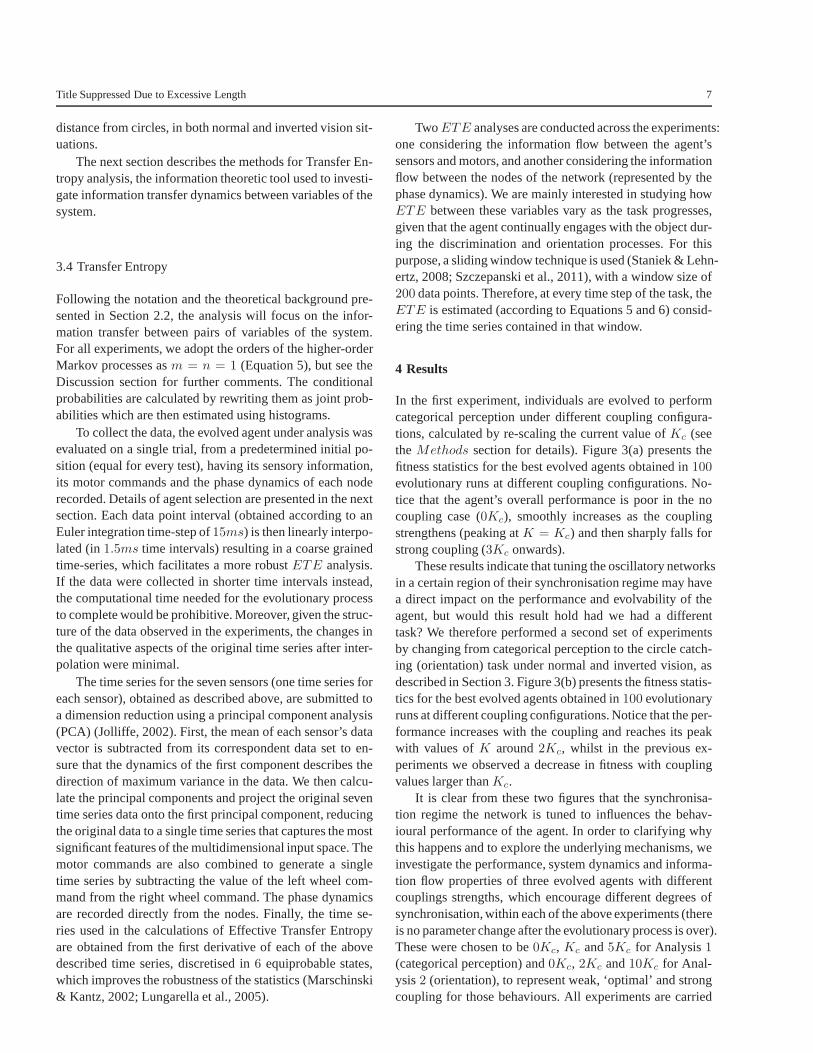
Consider Figure 6(a), which presents in its first row theaverage over time of the information flow between the oscil-latory nodes of the uncoupled network for the circle catching(first column) and square avoidance (second column) sce-narios, respectively, according to Equation 11:
T (n, n′) =1
Tw
Tw∑
w=1
[ETEw(n, n′) − ETEAw (n, n′)] (11)
where T (n, n′) is the average Effective Transfer EntropyETE between the pair of nodes(n, n′), estimated accord-ing to Equation 6,w is the time window andTw is totalnumber of windows. The superscriptA stands for theETEcalculated in the autonomous case.
As expected, the uncoupled network has almost noETEbetween nodes during most of the task, except when sen-sory readings modulate the ongoing phase activity, whichexplains why the few deviations from zero that occur arewith relation to nodes that have sensory inputs (recall thatonly even nodes receive sensory inputs, see Figure 3.1 fordetails). Observe that the flow between any two given nodesis not necessarily symmetric (e.g. there is a flow from node14 to 12 but the opposite is not true), as explained in Section2.2.
In theKc condition (Figure 6(a), second row), however,the coupling elicits a much broader modulation of the nodes’phase activity by the sensory inputs, stressing the internalcommunication between oscillators. The network is fullyconnected but nodes do not interact in the same way: theETE values between pairs of nodes vary according to thecorresponding sensory stimulus, the previous phase activity
of the nodes and its natural frequency. Also, notice that thesensory inputs not only increase the information flow withinthe network but also decrease it, reflecting a modulation ofthe spontaneous network phase activity (the activity the net-work would have without sensory inputs). Although Trans-fer Entropy always results in a positive measurement, recallfrom Section 3 that to highlight the sensory influence theabove results are obtained by subtracting theETE calcu-lated for the autonomous condition, hence the negative read-ings in the plots.
Compare the previous analysis with the5Kc condition(Figure 6(a), third row). As the network is strongly coupledand acts as a single giant oscillator, weak sensory stimuliof one or more nodes cannot promote a significant pertur-bation or change in the ongoing dynamics; in other words,the sensory readings do not contribute to the discriminationof the object given that different incoming stimuli throughother nodes would have little impact on the entrained net-work. Even though the system is able to detect the objectand generate a motor response to it, the categorization per-formance is impaired.
This diversity of information flow between the differentcoupling configurations follows the variation in the synchro-nisation index between nodes of the network, portrayed inFigure 6(b). The small level of synchronisation in the0Kc
network has a corresponding small flow of information be-tween nodes, and the large level of synchronisation in the5Kc network is accompanied by a reduced flow ofETE
between its nodes. The intermediate point, theKc network,has both a synchronisation regime and diverse and highlyasymmetric information dynamics.
In summary, although all configurations are fully con-nected, theKc network is able to use a great variety of flexi-ble, reconfigurable functional connections. Figure 6(c) illus-trate this fact by redrawing the connection scheme accordingto the magnitude of theETE between nodes - only nodeswith mean information flow50% above the global averageare connected. Notice the much richer connectivity in theKc condition than in the other two. The higher performanceand evolvability achieved by this configuration can thus beattributed to its nodes’ superior ability to communicate andorganise themselves functionally, resulting in a more effi-cient information flow between the ongoing network activ-ity, the agent’s body and the environmental context.
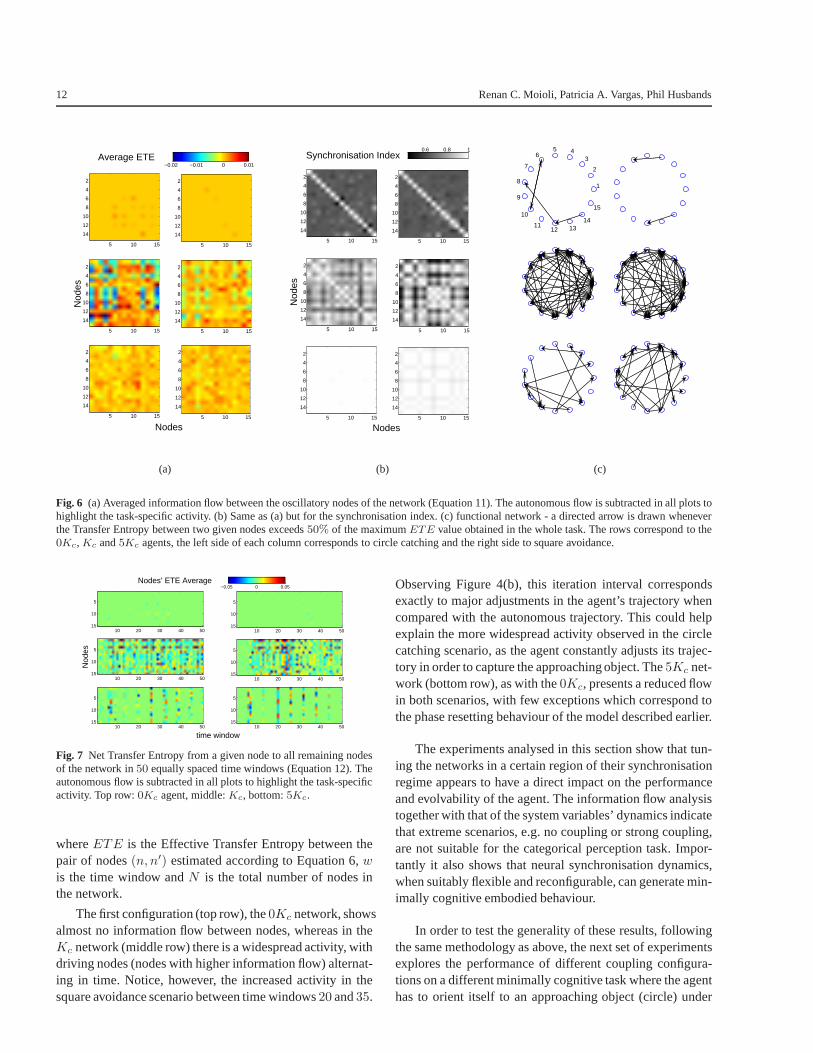
Figure 7 shows the temporal evolution of the net Trans-fer Entropy from a given node to all remaining nodes of thenetwork in50 equally spaced time windows, defined as thepreferred direction of information flow (Staniek & Lehnertz,2008):
T (n, n′, w) =1
N − 1
∑
n6=n′
[ETEn,n′(w) − ETEn′,n(w)]
(12)
12 Renan C. Moioli, Patricia A. Vargas, Phil Husbands
5 10 15
2
4
6
8
10
12
14
5 10 15
2
4
6
8
10
12
14
Nod
es
5 10 15
2
4
6
8
10
12
14
5 10 15
2
4
6
8
10
12
14
Nodes5 10 15
2
4
6
8
10
12
14
5 10 15
2
4
6
8
10
12
14
−0.02 −0.01 0 0.01Average ETE
(a)
5 10 15
2
4
6
8
10
12
14
5 10 15
2
4
6
8
10
12
14
Nod
es
5 10 15
2
4
6
8
10
12
14
5 10 15
2
4
6
8
10
12
14
5 10 15
2
4
6
8
10
12
14
Nodes5 10 15
2
4
6
8
10
12
14
0.6 0.8 1Synchronisation Index
(b)
2
6
7
8
9
10
11
345
12 1314
15
1
(c)
Fig. 6 (a) Averaged information flow between the oscillatory nodesof the network (Equation 11). The autonomous flow is subtracted in all plots tohighlight the task-specific activity. (b) Same as (a) but forthe synchronisation index. (c) functional network - a directed arrow is drawn wheneverthe Transfer Entropy between two given nodes exceeds50% of the maximumETE value obtained in the whole task. The rows correspond to the0Kc, Kc and5Kc agents, the left side of each column corresponds to circle catching and the right side to square avoidance.
Nod
es
10 20 30 40 50
5
10
1510 20 30 40 50
5
10
15
10 20 30 40 50
5
10
15
time window10 20 30 40 50
5
10
15
10 20 30 40 50
5
10
1510 20 30 40 50
5
10
15
−0.05 0 0.05Nodes’ ETE Average
Fig. 7 Net Transfer Entropy from a given node to all remaining nodesof the network in50 equally spaced time windows (Equation 12). Theautonomous flow is subtracted in all plots to highlight the task-specificactivity. Top row:0Kc agent, middle:Kc, bottom:5Kc.
whereETE is the Effective Transfer Entropy between thepair of nodes(n, n′) estimated according to Equation 6,wis the time window andN is the total number of nodes inthe network.
The first configuration (top row), the0Kc network, showsalmost no information flow between nodes, whereas in theKc network (middle row) there is a widespread activity, withdriving nodes (nodes with higher information flow) alternat-ing in time. Notice, however, the increased activity in thesquare avoidance scenario between time windows20 and35.
Observing Figure 4(b), this iteration interval correspondsexactly to major adjustments in the agent’s trajectory whencompared with the autonomous trajectory. This could helpexplain the more widespread activity observed in the circlecatching scenario, as the agent constantly adjusts its trajec-tory in order to capture the approaching object. The5Kc net-work (bottom row), as with the0Kc, presents a reduced flowin both scenarios, with few exceptions which correspond tothe phase resetting behaviour of the model described earlier.
The experiments analysed in this section show that tun-ing the networks in a certain region of their synchronisationregime appears to have a direct impact on the performanceand evolvability of the agent. The information flow analysistogether with that of the system variables’ dynamics indicatethat extreme scenarios, e.g. no coupling or strong coupling,are not suitable for the categorical perception task. Impor-tantly it also shows that neural synchronisation dynamics,when suitably flexible and reconfigurable, can generate min-imally cognitive embodied behaviour.
In order to test the generality of these results, followingthe same methodology as above, the next set of experimentsexplores the performance of different coupling configura-tions on a different minimally cognitive task where the agenthas to orient itself to an approaching object (circle) under

Title Suppressed Due to Excessive Length 13
0 10 20 30 40 50 60 70
−150
−100
−50
0
50
100
Task iteration time
Age
nt−
Obj
ect S
epar
atio
n
(a)
0 10 20 30 40 50 60 70
−150
−100
−50
0
50
Task iteration time
Age
nt−
Obj
ect S
epar
atio
n
(b)
0 10 20 30 40 50 60 70
−60
−40
−20
0
20
40
60
Task iteration time
Age
nt−
Obj
ect S
epar
atio
n
(c)
(ETEsm
− ETEms
) normal
10 20 30 40 50 60 70
−50
0
50
(ETEsm
− ETEms
) inverted
10 20 30 40 50 60 70
−50
0
50
Task Iteration Time
(d)
(ETEsm
− ETEms
) normal
10 20 30 40 50 60 70
−50
0
50
(ETEsm
− ETEms
) inverted
10 20 30 40 50 60 70
−50
0
50
Task Iteration Time
(e)
(ETEsm
− ETEms
) normal
10 20 30 40 50 60 70
−50
0
50
(ETEsm
− ETEms
) inverted
10 20 30 40 50 60 70
−50
0
50
−0.2
0
0.2
Task Iteration Time
(f)
Fig. 8 Top plots: generalisation performance of the agent over100 aleatory runs. The red colour is related to circle catching under normal visionand the blue colour to the inverted vision scenario. Green lines reflect the behaviour under autonomous network dynamics(clamped sensors). Theplots illustrate the value of the horizontal separation of the agent and the object. Bottom plots: difference between Effective Transfer Entropy fromsensors to motors,ETEsm, and from motors to sensors,ETEms, for each of the17 different initial horizontal displacements ([−50, 50]) that theagent is evaluated on during evolution (Section 3).ETE is calculated according to Equation 6. Figures refer to (a)(d)0Kc , (b)(e)2Kc and (c)(f)10Kc.
normal and inverted vision (see Section 3 for experimentalprocedures).
4.2 Analysis 2: Orientation under Normal and InvertedVision
Recall Figure 3(b), which presents the fitness statistics forthe best evolved agents obtained in100 evolutionary runsat different coupling configurations for task 2 (circle catch-ing with normal and inverted vision). The performance in-creases with the coupling and peaks atK = 2Kc, presentinga noticeable fall in performance for couplings greater than5Kc. The following analysis will therefore consider threeindividuals: one drawn from the0Kc scenario, one from the2Kc and one from the10Kc scenario, all with fitness val-ues close to the fitness median obtained on each respectivecoupling scenario set of results.
Observe Figures 8(a), 8(b) and 8(c), which present thegeneralisation performance of the agents (performance in100 aleatory trials after evolution). The agent controlled bythe uncoupled network (0Kc) cannot succeed in catchingcircles with either normal or inverted vision and all trajecto-ries seem to be a variation of the autonomous trajectory (il-lustrated by the green line in the plot) - there is almost no in-fluence from the sensory readings. The2Kc agent, however,
has good performance in both sensory modes, centring onthe object in slightly different ways as the task progresses,depending on whether it has normal or inverted vision, mak-ing fine adjustments to the trajectory towards the end. A sim-ilar strategy is employed by the very strongly coupled agent(10Kc), however the accuracy with which the agent centreson the object towards the end of the task is poor and thisdivergence explains the lower fitnesses obtained. Neverthe-less, both2Kc and10Kc agents display different behavioursfrom their autonomous trajectories, in contrast with the un-coupled network, indicating that they make use of the sen-sory information to solve the task.
An inspection of the dynamics of some of the systemvariables reveals that, as expected, the uncoupled networkhas some node activity varying directly with the sensoryreadings, with nodes without inputs keeping their naturalfrequency throughout the task (see Figure 9(a)). The syn-chronisation index remains low but has a significant vari-ance. The lack of internal coupling results in the absence ofany internal communication or flow of information as wellas any influence caused by acting on the environment. Asthe task is intrinsically ambiguous, the agent cannot performwell.
The2Kc network (Figure 9(b)), in contrast, remains syn-chronised for most of the time and the nodes can only “es-
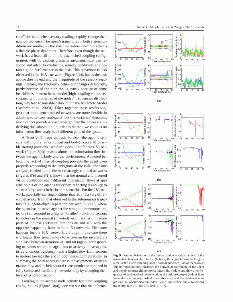
14 Renan C. Moioli, Patricia A. Vargas, Phil Husbands
cape” this state when sensory readings rapidly change theirnatural frequency. The agent’s trajectories in both visioncon-ditions are similar, but the synchronisation index plot revealsa diverse phase dynamics. Therefore, even though the net-work has a fixed, all-to-all pre-established coupling config-uration, with no explicit plasticity mechanisms, it can re-spond and adapt to conflicting sensory conditions and ob-tain a good performance in the task. This behaviour is alsoobserved in the10Kc network (Figure 9(c)), but as the taskapproaches its end and the magnitude of the sensory read-ings increase, the frequency behaviour changes drastically,partly because of the high inputs, partly because of someinstabilities inherent in the model (high coupling values,as-sociated with properties of the nodes’ frequencies distribu-tion, may lead to unstable behaviour in the Kuramoto Model(Acebron et al., 2005)). Taken together, these results sug-gest that more synchronised networks are more flexible inadapting to sensory ambiguity, but the variables’ dynamicsalone cannot provide a broader insight into the processes un-derlying this adaptation. In order to do that, we conduct aninformation flow analysis of different parts of the system.
A Transfer Entropy analysis between the agent’s sen-sors and motors (environment and body) across all possi-ble starting positions used during evolution for the0Kc net-work (Figure 8(d)) reveals almost no information flow be-tween the agent’s body and the environment. As noted be-fore, the lack of internal coupling prevents the agent fromproperly responding to the ambiguity of the task. The sameanalysis, carried out on the more strongly coupled networks(Figures 8(e) and 8(f)), shows that the normal and invertedvision conditions elicit different information flows at spe-cific points of the agent’s trajectory, reflecting its ability tosuccessfully catch circles in both scenarios. For the2Kc net-work, especially, starting positions that require a very differ-ent behaviour from that observed in the autonomous trajec-tory (e.g. agent-object separation between[−50, 0], wherethe agent has to move against the straight autonomous tra-jectory) correspond to a higher (smaller) flow from sensorsto motors in the normal (inverted) vision scenario in someparts of the task (between iterations30 and 40), with theopposite happening from iteration50 onwards. The samehappens for the10Kc network, although in this case thereis a higher flow from motors to sensors in the inverted vi-sion case between iterations40 and60 (again, correspond-ing to points where the agent has to actively move againstits autonomous trajectory), and a higher flow from sensorsto motors towards the end in both vision configurations. Insummary, the point to stress here is the asymmetry of infor-mation flow and its behavioural correspondence obtained infully connected oscillatory networks only by changing theirlevel of synchronisation.
Looking at the average node activity for these couplingconfigurations (Figure 10(a)), one can see that the informa-
0 20 40 60 800
50
100
150
Age
nt/O
bjec
t Sep
arat
ion
0 20 40 60 80−40
−20
0
20
40
Task iteration time
Nod
es F
requ
ency
0 20 40 60 800
0.2
0.4
0.6
0.8
1
Syn
chro
nisa
tion
inde
x
0 20 40 60 8040
60
80
100
120
140
Age
nt/O
bjec
t Sep
arat
ion
0 20 40 60 80−40
−20
0
20
40
Task iteration time
Nod
es F
requ
ency
0 20 40 60 800
0.2
0.4
0.6
0.8
1
Syn
chro
nisa
tion
inde
x
(a)
0 20 40 60 800
20
40
60
80
100A
gent
/Obj
ect S
epar
atio
n
0 20 40 60 80−80
−60
−40
−20
0
20
Task iteration time
Nod
es F
requ
ency
0 20 40 60 800.8
0.85
0.9
0.95
1
Syn
chro
nisa
tion
inde
x
0 20 40 60 800
20
40
60
80
100
Age
nt/O
bjec
t Sep
arat
ion
0 20 40 60 80−100
−50
0
50
Task iteration time
Nod
es F
requ
ency
0 20 40 60 800.8
0.85
0.9
0.95
1
Syn
chro
nisa
tion
inde
x
(b)
0 20 40 60 8050
100
150
200
Age
nt/O
bjec
t Sep
arat
ion
0 20 40 60 80−200
−100
0
100
200
300
Task iteration time
Nod
es F
requ
ency
0 20 40 60 800.4
0.6
0.8
1
Syn
chro
nisa
tion
inde
x
0 20 40 60 8050
100
150
200
Age
nt/O
bjec
t Sep
arat
ion
0 20 40 60 80−150
−100
−50
0
50
Task iteration time
Nod
es F
requ
ency
0 20 40 60 800.4
0.6
0.8
1
Syn
chro
nisa
tion
inde
x
(c)Fig. 9 Detailed behaviour of the internal and external dynamics for theorientation task agents. The top (bottom) three graphics ofeach figurerefer to the circle catching under normal (inverted) visionbehaviour.The leftmost column illustrates the horizontal coordinateof the agentand the object (straight horizontal lines), the middle one shows the fre-quency of each node of the network as the task progresses (colour linesfor nodes with inputs, dashed lines otherwise) and the rightmost onespresent the synchronisation index. Green lines reflect the autonomoustrajectory. (a)0Kc, (b) 2Kc and (c)10Kc.

Title Suppressed Due to Excessive Length 15
5 10 15
2
4
6
8
10
12
14
5 10 15
2
4
6
8
10
12
14
Nod
es
5 10 15
2
4
6
8
10
12
14
5 10 15
2
4
6
8
10
12
14
5 10 15
2
4
6
8
10
12
14
Nodes
5 10 15
2
4
6
8
10
12
14
0 0.01 0.02Average ETE
(a)
5 10 15
2
4
6
8
10
12
14
Nodes5 10 15
2
4
6
8
10
12
14
5 10 15
2
4
6
8
10
12
14
5 10 15
2
4
6
8
10
12
14
Nod
es
5 10 15
5
10
155 10 15
2
4
6
8
10
12
14
0.6 0.8 1Synchronisation Index
(b)
1
2
345
6
7
8
9
10
1112 13
14
15
(c)
Fig. 10 (a) Averaged information flow between the oscillatory nodesof the network (Equation 11). The autonomous flow is subtracted in all plotsto highlight the task-specific activity. (b) Same as (a) but for the synchronisation index. (c) functional network - a directed arrow is drawn wheneverthe Transfer Entropy between two given nodes exceeds50% of the maximumETE value obtained in the whole task. The rows correspond (top tobottom) to the0Kc, 2Kc and10Kc agents. The left side of each column refers to orientation with normal vision, the right to inverted vision.
tion flow under normal and inverted vision is similar, withvery little activity for the uncoupled network, whereas themore strongly coupled agents (2Kc and 10Kc), althoughhaving a nearly identical trajectory when catching the cir-cles with normal and inverted vision in each correspondingscenario, show variation in their internal nodes’ informationflow. Having only the environmental feedback to shape itsbehaviour, the0Kc network fails to detect and respond prop-erly to this conflicting situation because the phase dynamicsof each node can only be altered by the external stimulus,which in this case is made ambiguous, while the internal ac-tivity of the2Kc and the10Kc networks is modulated by theenvironmental context - the conflicting readings result in dif-ferent phase dynamics that are exploited to generate fit be-haviour. The synchronisation index adds to that perspectiveby showing that although highly synchronised, the2Kc net-work is still flexible enough to escape the nearly entrainedstate of the10Kc network or the incoherent behaviour of theuncoupled framework, producing the fittest agent.
With these two plots in mind, observe the picture ofthe equivalent functional network for the chosen agents inthis task (Figure 10(c)). There are richer functional con-nections between nodes in the2Kc network not only whencomparing across different coupling configurations but alsobetween the two vision conditions (inverted vision uses a
denser set of functional connections than normal vision).This higher performing network is more able to reconfig-ure its internal functional architecture than its counterparts,allowing it to cope well with both conditions.
Figure 11 shows the temporal evolution of the net Trans-fer Entropy between nodes (Equation 12). It reveals the ab-sence of significant readings in the uncoupled network butshows much higher levels in the2Kc network as the taskprogresses, with the10Kc network having alternating mo-ments of high and low readings. This plot provides a differ-ent angle of analysis on our system by making evident thedifferences in the flow of information within the differentnetworks and hence in the relationships between the nodesin the various contexts. Given that the phase difference dy-namics captures all the effective dynamics of the KuramotoModel (Maistrenko et al., 2005), it’s possible to see how dif-ferent functional networks emerge from the interaction withthe environment within the same coupling condition, stress-ing adaptability, or across different coupling conditions, re-vealing aspects of functional structure dependent on degreeof coupling.
Comparing Figures 8(e) and 8(f) with Figure 11, noticehow the magnitude of theETEsm andETEms flows arehigh at particular moments of the task in the2Kc agent,whilst theETE between nodes has noticeable deviations

16 Renan C. Moioli, Patricia A. Vargas, Phil Husbands
from zero across the trial. There is, therefore, no clear sim-ilarity between the sensorimotor and the network’s nodesphase activity information flow. In the10Kc network, how-ever, the higher variability of the flow between nodes have acorrespondence in theETEsm andETEms flow. This cor-respondence can be explained by the higher value of cou-pling between nodes in the sense that the sensorimotor ac-tivity perturbs a much more rigid framework, driving allnodes’ behaviour. The2Kc network is more loosely coupledso that the perturbations modulate and influence the nodes’behaviour, but do not ultimately determine it.
In summary, the previous experiments with categoricalperception revealed a limitation of both weakly and stronglycoupled networks in achieving good performance in discrim-inating objects with different shapes. The second experimentwith orientation in normal and inverted vision conditionsshows that the weakly coupled network continues to fail ina conflicting scenario, but the more strongly coupled net-works succeed. The conclusion is that, for our framework,networks with high synchronisation levels are able to de-tect and respond to visual stimuli but struggle to exploitthe environmental context. In other words, the highly syn-chronised structures evolved here can detect (even with al-tered vision) but not discriminate among different externalstimuli. In both tasks, networks with ’intermediate’ levelsof coupling (and hence propensity for synchronisation) per-form best as this provides a more fluid, flexible network ableto reconfigure and adapt to different behavioural conditions.However, as we have seen, this optimal ’intermediate’ levelis significantly different for the two tasks.
5 Discussion
Current research on neurophysiologicalprocesses shows thatoscillatory neural activity is closely related to cognition andbehaviour, with synchronisation mechanisms playing a keyrole in the integration and functional organization of differ-ent cortical areas (Varela et al., 2001; Engel et al., 2001;Womelsdorf et al., 2007). Nevertheless, its informationalcon-tent and relationship with behaviour - and hence cognition -are still to be fully understood (Rieke et al., 1997; Mazzoniet al., 2008; Deco et al., 2011; Flanders, 2011).
In this context, following an Evolutionary Robotics ap-proach, we evolved simulated robotic agents controlled bya spontaneously rhythmic network of coupled phase oscil-lators, showing that their performances in variations of acategorical perception task depend on the synchronisationregime of the network. This was also shown to be the casefor an orientation task under normal and inverted vision, butthe dependence on the synchronisation regime was quite dif-ferent from in the first task. The analysis focused both on abehavioural level description, investigating the agent/objecttrajectories, and on a mechanism level description, exploring
10 20 30 40 50
5
10
1510 20 30 40 50
5
10
15
Nod
es
10 20 30 40 50
5
10
1510 20 30 40 50
5
10
15
10 20 30 40 50
5
10
15
time window
10 20 30 40 50
5
10
15
−0.05 0 0.05Nodes’ ETE Average
Fig. 11 Net Transfer Entropy from a given node to all remaining nodesof the network in50 equally spaced time windows (Equation 12). Theautonomous flow is subtracted in all plots to highlight the task-specificactivity. The rows correspond (top to bottom) toKc, 2Kc and10Kc
agents. The left column is for normal vision and the right forinvertedvision.
the dynamics and the information transfer properties withinand between the agent and the environment.
The design of the experimental framework attempted tocapture relevant properties of its biological counterparts thatwould suit the aims of our study. The network model is in-spired by the Kuramoto Model of coupled phase oscilla-tors whilst the robotics approach explores the enactive na-ture of sensory and cognitive processes. Our focus is onthree aspects: the information flow between sensors and mo-tors, capturing the body/environment interaction; the aver-age flow between nodes of the network, stressing the inter-nal communication; and the evolution in time of the averagenet flow from a given node to all its counterparts, revealingat various moments of the task a higher/lower participationin the overall information dynamics.
The first experiment explored the fitness variation ofevolved individuals under different network couplingsK fora categorical perception task. The results showed that thereis a statistically significant difference in performance for dif-ferent strengths of coupling, with the best fitness evolutionperformance obtained whenK = Kc, the critical value.Although the term “critical” here is not directly related toits meaning for self-organised criticality (Beggs, 2008),pre-vious work (Kitzbichler et al., 2009) showed that the Ku-ramoto Model presents properties of critical systems (e.g.greater information transmission, storage, sensitivity to ex-ternal stimulus) when its coupling is tuned to the criticalvalue (Equation 4). Our results confirm this for the categor-ical perception task.
For the agent with best performance (K = Kc), the dy-namical analysis shows that there is a very rich phase be-haviour in the critical coupled network, with nodes oscillat-ing at a variety of frequencies, occasionally synchronisingand forming independent functionally connected clusters.Inthe Effective Transfer Entropy (ETE) analysis, we noticea higher flow magnitude in the sensorimotor loop time se-

Title Suppressed Due to Excessive Length 17
ries (ETEsm andETEms), which has a behavioural corre-spondence and relates to sharper adjustments in the agent’strajectory, suggesting that the agent is more able to convertsensory information into motor responses to maximize itsperformance; we also observe a much broader internal com-munication between oscillators, with a great variety of func-tional connections in comparison with other coupling con-figurations. Remarkably, even though the network is fullyconnected, the flow is not symmetric, and the higher perfor-mance of the critical coupled network can be linked to itsflexible ongoing dynamics which can be modulated by theenvironmental context.
The second experiment studied orientation to falling cir-cles under normal and inverted vision, particularly interest-ing for presenting to the agent an ambiguous and conflictingscenario.
We found that the performance increases with the de-gree of coupling, but this time reaches its peak between2and 4Kc, decreasing for the very strong coupling valuesgreater than that. We compared three evolved individuals,one with no coupling (0Kc), one with strong coupling (2Kc)and the other with very strong coupling (10Kc) between os-cillators. The first is unable to succeed on the task whilstthe 2 and10Kc agents produce good performance in bothsensory modes, with the2Kc agent outperforming the verystrongly coupled one.
Dynamical analysis shows that the2Kc network rapidlysynchronises, with some nodes escaping the entrained stateonly when the corresponding sensory input is large. How-ever, there is a diverse phase dynamics, with conflicting val-ues resulting in different phase dynamics that are exploitedto generate fit behaviour that can cope with the different vi-sual conditions. Therefore, even though the network has afixed, all-to-all pre-established coupling configuration,withno explicit plasticity mechanisms, it can respond and adaptto conflicting sensory conditions and obtain good perfor-mance on the task. This is further stressed by the Trans-fer Entropy analysis which shows that the normal and in-verted vision conditions elicit a difference in the informationflow at specific points of the agent’s trajectory. The resultshighlight the asymmetry of information flow and its behav-ioural correspondence obtained in fully connected oscilla-tory networks only by changing their level of synchronisa-tion. Hence, the results suggest that synchronised networkswith an ’intermediate’ level of coupling are more able to re-configure functional connections not only when comparingacross different coupling configurations but also between thetwo vision conditions, reflecting its superior performanceonthe task.
Concluding our analysis for both experiments, considerFigures 12(a) and 12(b), which display the formation of groupsof oscillators during the execution of the task for the selectedcoupling conditions for Experiments1 and2, respectively.
The network has initially15 single-node “clusters”, eachcorresponding to an oscillator. A group (cluster) is mergedwhenever the phase difference between two given nodes isbelow a certain threshold (chosen to be1 here) and the fre-quencies are similar (less than1Hz apart). Hence valuesvary from 1 (single, giant cluster containing all the oscil-lators) to15 (single-node clusters).
In the first experiment, the uncoupled network is associ-ated with a large number of single-node groups, whereas thestrongly coupled network has only one big group throughnearly all of the task, indicating complete synchronisation.Curiously, the critically coupled network alternates betweenthese two extremes. The same behaviour is observed for Ex-periment2, with the exception that the very strong couplednetwork desynchronises at the end of the task, as revealedby earlier analysis. These plots reinforce an important as-pect raised in the Introduction and mentioned throughoutthe paper: synchronisation dynamics modulate the assembly,collapse and reconfiguration of functional sub-networks. Inour experiments, a higher diversity of such assemblies arepresent in the top performing agents, linking the adaptabilityof the agent to the flexibility of its functional connections.
The previous analysis is complemented by Figures 12(c)and 12(d), which present the dynamics of a metastability in-dexλ and the Largest Lyapunov Exponent (LLE) for thechosen scenarios.λ (Equation 13) is calculated as the esti-mated variance of the synchronisation indexr (Eq. 3) overall time pointst = 1 . . . T and reflect the diversity of syn-chronisation states obtained for each coupling configurationof the network (Shanahan, 2010).
λ =1
T − 1
T∑
t=1
(r(t)− < r >T )2 (13)
The Largest Lyapunov Exponent, calculated using thephase variablesθi, i = 1 . . .N (Maistrenko et al., 2005),indicate how chaotic the phase dynamics - and hence oursystem - are. To obtain theLLE, we followed the methoddescribed in Rosenstein et al. (1993) which is specially de-signed to be robust and fast in small data sets.
In both experiments, we notice that the metastability de-creases (as expected) as the coupling increases, showing thatthere is less variation in the synchronisation index. The dy-namics of the number of groups relate to the metastabilityindex, with the critically coupled network also appearing inan intermediate position. An interesting point for the criticalcoupling condition is to notice how the agent/environmentinteraction in the categorical perception task reduces thespon-taneous chaoticity level of the network (calculated for theautonomous network dynamics), whereas in the inverted vi-sion scenario, near the critical coupling, chaotic behaviouris more prominent when the agent is engaged in the taskthan when under the influence of the autonomous network

18 Renan C. Moioli, Patricia A. Vargas, Phil Husbands
0 20 40 60 800
5
10
15
20
Task iteration time
Num
ber
of G
roup
s
0 20 40 60 800
5
10
15
20
0Kc
Kc
5Kc
0Kc
Kc
5Kc
(a)
0 20 40 60 800
5
10
15
20
0 20 40 60 800
5
10
15
20
Task iteration time
Num
ber
of G
roup
s
0Kc
2Kc
10Kc
0Kc
2Kc
10Kc
(b)
−1 0 1 2 3 4 5 60
0.01
0.02
0.03
0.04
0.05
Coupling Factor (xKc)
λ circleλ squareLLE
c
LLEs
LLEa
(c)
0 2 4 6 8 100
0.01
0.02
0.03
0.04
0.05
0.06
0.07
Coupling Factor (xKc)
λ normalλ invertedLLE
c
LLEs
LLEa
(d)
Fig. 12 Clustering of oscillators and metastable states for different coupling conditions as the task progresses. (a) and (b):nodes that have similarfrequencies and a phase shift below a small threshold are grouped. Values vary from1 (single, giant cluster containing all the oscillators) to15(single-node clusters). (c): metastability indexλ (Equation 13) superposed with the Largest Lyapunov Exponent (LLE) for the circle (LLEc),square (LLEs) and autonomous (LLEa) configurations. Largerλ indicates a great diversity of synchronisation states in the network as thetask progresses;LLE greater than0 suggests chaotic dynamics. (d): same as (c), but for the normal vision, inverted vision and autonomousconfigurations. Figures (a) and (c) refer to Experiment1 and Figures (b) and (d) refer to Experiment2.
dynamics. Also, note that the Largest Lyapunov Exponentis close to zero in the uncoupled autonomous scenario forboth tasks (0Kc). This is anticipated and due to the lack ofexternal stimulus, which makes each node of the networkoscillate independently in a quasiperiodic way. The senso-rimotor coupling changes this behaviour (even without con-nections between nodes, coupling can be seen as occurring“indirectly” through the environment), and the network ac-tivity becomes more chaotic. Therefore, the above observa-tions reflect the adaptability and modulation of the networkactivity previously noticed in the information flow analysis.It also suggests that although neural synchronisation clearlyplays an important role in the generation of behaviour in thefittest agents, other kinds of transient dynamics are also ex-ploited (Santos et al., 2011).
There are some limitations for the framework presentedhere. Starting with the network model, the original formu-lation of the Kuramoto Model doesn’t take into account im-portant properties of real nervous systems (e.g. spatial dis-tribution of units, transmission delays, asymmetrical inter-actions), therefore an important step towards a more bio-logically plausible architectures would be to implement ex-tended versions of the model which tackle some of theseconstraints (Tass, 2006; Cumin & Unsworth, 2007; Break-spear et al., 2010). These extensions may also unfold morecomplex, metastable dynamics which are intrinsically con-nected to dynamic pattern formation in brain activity andhence are fundamental to adaptive behaviour (Omelchenkoet al., 2008; Tognoli & Kelso, 2009; Chialvo, 2010; Shana-han, 2010). As for the task scenarios, the experiments wereconducted following an evolutionary robotics approach which,
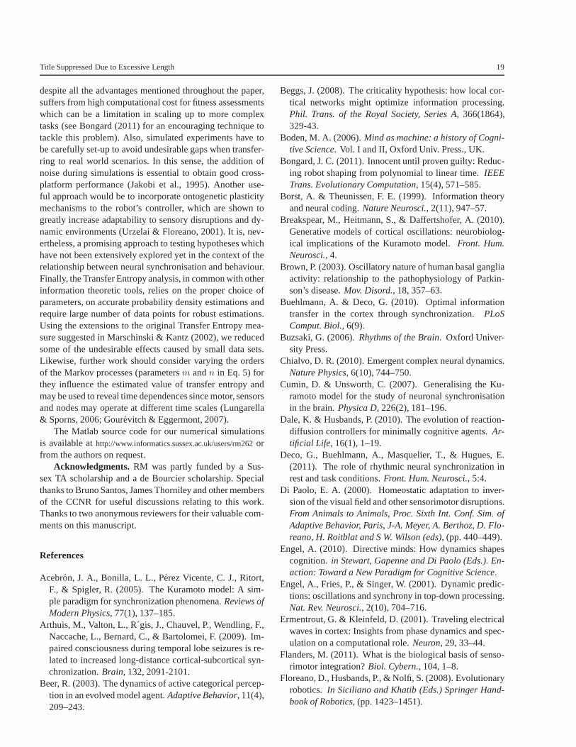
Title Suppressed Due to Excessive Length 19
despite all the advantages mentioned throughout the paper,suffers from high computational cost for fitness assessmentswhich can be a limitation in scaling up to more complextasks (see Bongard (2011) for an encouraging technique totackle this problem). Also, simulated experiments have tobe carefully set-up to avoid undesirable gaps when transfer-ring to real world scenarios. In this sense, the addition ofnoise during simulations is essential to obtain good cross-platform performance (Jakobi et al., 1995). Another use-ful approach would be to incorporate ontogenetic plasticitymechanisms to the robot’s controller, which are shown togreatly increase adaptability to sensory disruptions and dy-namic environments (Urzelai & Floreano, 2001). It is, nev-ertheless, a promising approach to testing hypotheses whichhave not been extensively explored yet in the context of therelationship between neural synchronisation and behaviour.Finally, the Transfer Entropy analysis, in common with otherinformation theoretic tools, relies on the proper choice ofparameters, on accurate probability density estimations andrequire large number of data points for robust estimations.Using the extensions to the original Transfer Entropy mea-sure suggested in Marschinski & Kantz (2002), we reducedsome of the undesirable effects caused by small data sets.Likewise, further work should consider varying the ordersof the Markov processes (parametersm andn in Eq. 5) forthey influence the estimated value of transfer entropy andmay be used to reveal time dependences since motor, sensorsand nodes may operate at different time scales (Lungarella& Sporns, 2006; Gourevitch & Eggermont, 2007).
The Matlab source code for our numerical simulationsis available athttp://www.informatics.sussex.ac.uk/users/rm262orfrom the authors on request.
Acknowledgments. RM was partly funded by a Sus-sex TA scholarship and a de Bourcier scholarship. Specialthanks to Bruno Santos, James Thorniley and other membersof the CCNR for useful discussions relating to this work.Thanks to two anonymous reviewers for their valuable com-ments on this manuscript.
References
Acebron, J. A., Bonilla, L. L., Perez Vicente, C. J., Ritort,F., & Spigler, R. (2005). The Kuramoto model: A sim-ple paradigm for synchronization phenomena.Reviews ofModern Physics, 77(1), 137–185.
Arthuis, M., Valton, L., R´gis, J., Chauvel, P., Wendling, F.,Naccache, L., Bernard, C., & Bartolomei, F. (2009). Im-paired consciousness during temporal lobe seizures is re-lated to increased long-distance cortical-subcortical syn-chronization.Brain, 132, 2091-2101.
Beer, R. (2003). The dynamics of active categorical percep-tion in an evolved model agent.Adaptive Behavior, 11(4),209–243.
Beggs, J. (2008). The criticality hypothesis: how local cor-tical networks might optimize information processing.Phil. Trans. of the Royal Society, Series A, 366(1864),329-43.
Boden, M. A. (2006).Mind as machine: a history of Cogni-tive Science. Vol. I and II, Oxford Univ. Press., UK.
Bongard, J. C. (2011). Innocent until proven guilty: Reduc-ing robot shaping from polynomial to linear time.IEEETrans. Evolutionary Computation, 15(4), 571–585.
Borst, A. & Theunissen, F. E. (1999). Information theoryand neural coding.Nature Neurosci., 2(11), 947–57.
Breakspear, M., Heitmann, S., & Daffertshofer, A. (2010).Generative models of cortical oscillations: neurobiolog-ical implications of the Kuramoto model.Front. Hum.Neurosci., 4.
Brown, P. (2003). Oscillatory nature of human basal gangliaactivity: relationship to the pathophysiology of Parkin-son’s disease.Mov. Disord., 18, 357–63.
Buehlmann, A. & Deco, G. (2010). Optimal informationtransfer in the cortex through synchronization.PLoSComput. Biol., 6(9).
Buzsaki, G. (2006).Rhythms of the Brain. Oxford Univer-sity Press.
Chialvo, D. R. (2010). Emergent complex neural dynamics.Nature Physics, 6(10), 744–750.
Cumin, D. & Unsworth, C. (2007). Generalising the Ku-ramoto model for the study of neuronal synchronisationin the brain.Physica D, 226(2), 181–196.
Dale, K. & Husbands, P. (2010). The evolution of reaction-diffusion controllers for minimally cognitive agents.Ar-tificial Life, 16(1), 1–19.
Deco, G., Buehlmann, A., Masquelier, T., & Hugues, E.(2011). The role of rhythmic neural synchronization inrest and task conditions.Front. Hum. Neurosci., 5:4.
Di Paolo, E. A. (2000). Homeostatic adaptation to inver-sion of the visual field and other sensorimotor disruptions.From Animals to Animals, Proc. Sixth Int. Conf. Sim. ofAdaptive Behavior, Paris, J-A. Meyer, A. Berthoz, D. Flo-reano, H. Roitblat and S W. Wilson (eds), (pp. 440–449).
Engel, A. (2010). Directive minds: How dynamics shapescognition. in Stewart, Gapenne and Di Paolo (Eds.). En-action: Toward a New Paradigm for Cognitive Science.
Engel, A., Fries, P., & Singer, W. (2001). Dynamic predic-tions: oscillations and synchrony in top-down processing.Nat. Rev. Neurosci., 2(10), 704–716.
Ermentrout, G. & Kleinfeld, D. (2001). Traveling electricalwaves in cortex: Insights from phase dynamics and spec-ulation on a computational role.Neuron, 29, 33–44.
Flanders, M. (2011). What is the biological basis of senso-rimotor integration?Biol. Cybern., 104, 1–8.
Floreano, D., Husbands, P., & Nolfi, S. (2008). Evolutionaryrobotics. In Siciliano and Khatib (Eds.) Springer Hand-book of Robotics, (pp. 1423–1451).

20 Renan C. Moioli, Patricia A. Vargas, Phil Husbands
Floreano, D. & Keller, L. (2010). Evolution of adaptive be-haviour in robots by means of Darwinian selection.PLoSBiology, 8(1).
Floreano, D. & Mattiussi, C. (2008).Bio-Inspired ArtificialIntelligence. MIT Press.
Glass, L. (2001). Rhythmic processes in physiology.Nature410 277-284.
Gourevitch, B. & Eggermont, J. (2007). Evaluating informa-tion transfer between auditory cortical neurons.J. Neuro-physiol.
Harnad, S. e. (1987).Categorical Perception: The Ground-work of Cognition.Cambridge University Press.
Harvey, I., Di Paolo, E., Wood, R., Quinn, M., & Tuci, E.(2005). Evolutionary robotics: A new scientific tool forstudying cognition.Artificial Life, 11(1-2), 79–98.
Hatsopoulos, N., Ojakangas, C., Paninski, L., & Donoghue,J. (1998). Information about movement direction ob-tained from synchronous activity of motor cortical neu-rons. Proc. Natl. Acad. Sci. USA, Neurobiology, 95,1570615711.
Husbands, P. (2009). Never mind the iguana, what about thetortoise? Models in adaptive behaviour.Adaptive Behav-ior, 17(4), 320–324.
Husbands, P., Smith, T., Jakobi, N., & O Shea, M. (1998).Better living through chemistry: Evolving GasNets forrobot control.Connection Science, 10, 185–210.
Ijspeert, A., Crespi, A., Ryczko, D., & Cabelguen, J. (2005).From swimming to walking with a salamander robotdriven by a spinal cord model.Science, 315(5817), 1416–1420.
Izhikevich, E. (1999). Weakly pulse-coupled oscillators,FMinteractions, synchronization, and oscillatory associativememory.IEEE Trans. Neural Networks, 10(3), 508–526.
Izquierdo, E. (2008). The dynamics of learning behaviour:a situated, embodied, and dynamical systems approach.PhD thesis, CCNR, University of Sussex.
Jackson, A., Gee, V., Baker, S., & Lemon, R. (2003). Syn-chrony between neurons with similar muscle fields inmonkey motor cortex.Neuron, 38, 115–125.
Jakobi, N., Husbands, p., & Harvey, I. (1995). Noise andthe reality gap: the use of simulations in evolutionaryrobotics. In Proc. 3rd European Conference on ArtificialLife. F. Moran et al. (Eds.), (pp. 704–720).
Jolliffe, I. T. (2002). Principal Component Analysis.Springer-Verlag New York.
Katz, P. E. (1999).Beyond Neurotransmission: Neuromodu-lation and its Importance for Information Processing.Ox-ford University Press.
Kitzbichler, M., Smith, M., Christensen, S., & Bullmore, E.(2009). Broadband criticality of human brain networksynchronization.PLoS Comput. Biol., 5(3).
Kullback, S. (1959).Information Theory and Statistics. Wi-ley, New York.
Kunyosi, M. & Monteiro, L. (2009). Recognition of noisyimages by PLL networks.Signal Processing, 89.
Kuramoto, Y. (1984). Chemical Oscillation, Waves, andTurbulence. Springer, New York.
Li, Z. & Hopfield, J. (1989). Modeling the olfactory bulband its neural oscillatory processings.Biol. Cybern.,61(5).
Lungarella, M., Ishiguro, K., Kuniyoshi, Y., & Otsu, N.(2007a). Methods for quantifying the causal structure ofbivariate time series.Int. J. of Bifurcation and Chaos,17(3):903-921.
Lungarella, M., Pegors, T., Bulwinkle, D., & Sporns, O.(2005). Methods for quantifying the informational struc-ture of sensory and motor data.Neuroinformatics, 3 (3),pp. 243-262.
Lungarella, M., Pitti, A., & Kuniyoshi, Y. (2007b). Infor-mation transfer at multiple scales.Physical Review E,056117.
Lungarella, M. & Sporns, O. (2006). Mapping informa-tion flow in sensorimotor networks.PLoS Comput. Biol.,2(10):e144.
Maistrenko, Y. L., Popovych, O. V., & Tass, P. A. (2005).Chaotic attractor in the Kuramoto Model.Int. J. of Bifur-cation and Chaos, 15(11), 34573466.
Marschinski, R. & Kantz, H. (2002). Analysing the infor-mation flow between financial time series: An improvedestimator for transfer entropy.The European PhysicalJournal B, 30 (2), p.275-281.
Mazzoni, A., Panzeri, S., Logothetis, N. K., & Brunel, N.(2008). Encoding of naturalistic stimuli by local fieldpotential spectra in networks of excitatory and inhibitoryneurons.PLoS Comput. Biol., 4(12).
McDonnell, M., Ikeda, S., & Manton, J. (2011). An in-troductory review of information theory in the context ofcomputational neuroscience.Biol. Cybern., 105, 55–70.
Murray, J. D. (1989).Mathematical Biology: An Introduc-tion. Springer-Verlag Berlin Heidelber.
Noe, A. (2004).Action in perception.Cambridge, MA: MITPress.
Omelchenko, O., Maistrenko, Y., & Tass, P. (2008). Chimerastates: The natural link between coherence and incoher-ence.Phys. Rev. Lett., 100, 044105.
Pfeifer, R., Lungarella, M., & Iida, F. (2007). Self-organization, embodiment, and biologically inspiredrobotics.Science 318 1088.
Pikovsky, A., Rosenblum, M., & Kurths, J. (2001).Syn-chronization: A Universal Concept in Nonlinear Sciences.Cambridge University Press.
Pitti, A., Lungarella, M., & Kuniyoshi, Y. (2009). Generat-ing spatiotemporal joint torque patterns from dynamicalsynchronization of distributed pattern generators.Front.NeuroRobotics, 3:2, 1–14.

Title Suppressed Due to Excessive Length 21
Pitti, A., Niiyama, R., & Kuniyoshi, Y. (2010). Creatingand modulating rhythms by controlling the physics of thebody.Autonomous Robots, 28:3, pp. 317-329.
Rieke, F., Warland, D., van Steveninck, R. R., & Bialek, W.(1997). Spikes: Exploring the Neural Code. BradfordBook - MIT Press, Cambridge MA.
Rolls, E. T. & Treves, A. (1998).Neural networks and brainfunction. Oxford University Press.
Rosenstein, M., Collins, J., & Deluca, C. (1993). A practicalmethod for calculating largest Lyapunov exponents fromsmall data sets.Physica D: Nonlinear Phenomena, 65(1-2), 117–134.
Santos, B., Barandiaran, X., & Husbands, P. (2011).Metastable dynamical regimes in an oscillatory networkmodulated by an agent’s sensorimotor loop.Proc. IEEESymposium on Artificial Life (SSCI).
Schreiber, T. (2000). Measuring information transfer.Phys.Rev. Lett., 85, 461464.
Shanahan, M. P. (2010). Metastable chimera states incommunity-structured oscillator networks.Chaos, 20,013108.
Silverman, B. (1998).Density Estimation for Statistics andData Analysis. London: Chapman and Hall.
Singer, W. (1993). Synchronization of cortical activity andits putative role in information processing and learning.Annu. Rev. Physiology, 55, 349–374.
Singer, W. (1999). Neuronal synchrony: a versatile code forthe definition of relations?Neuron, 24(1), 49–65.
Staniek, M. & Lehnertz, K. (2008). Symbolic transfer en-tropy. Phys. Rev. Lett., 100 (15).
Stewart, J., Gapenne, O., & Di Paolo, E. E. (2010).Enac-tion: Toward a New Paradigm for Cognitive Science.MITPress.
Strogatz, S. (2000). From Kuramoto to Crawford: exploringthe onset of synchronization in populations of coupled os-cillators. Physica D, 143.
Szczepanski, J., Arnold, M., Wajnryb, E., Amigo, J. M., &Sanchez-Vives, M. V. (2011). Mutual information andredundancy in spontaneous communication between cor-tical neurons.Biol. Cybern., 104, 161–174.
Taga, G. (1994). Emergence of bipedal locomotion throughentrainment among the neuro-musculo-skeletal systemand the environment.Physica D, 75(1-3), 190–208.
Tass, P. (2006).Phase resetting in medicine and biology:stochastic modelling and data analysis. Springer.
Tognoli, E. & Kelso, J. A. S. (2009). Brain coordinationdynamics: True and false faces of phase synchrony andmetastability.Prog. Neurobiol., 87(1), 31–40.
Urzelai, J. & Floreano, D. (2001). Evolution of adaptivesynapses: Robots with fast adaptive behavior in new en-vironments.Evol. Comput., 9(4), 495–524.
Varela, F., Lachaux, J., Rodriguez, E., & Martinerie, J.(2001). The brainweb: phase synchronization and large-scale integration.Nat. Rev. Neurosci., 2(4).
Vicente, R., Wibral, M., Lindner, M., & Pipa, G. (2011).Transfer entropy: a model-free measure of effective con-nectivity for the neurosciences.J. Comput. Neurosci., 30,4567.
von der Malsburg, C. (1981). The correlation theory of thebrain. Internal report. Max-Planck-Institute for Biophys-ical Chemistry, Gottingen, Germany.
Williams, P. & Beer, R. (2010). Information dynamics ofevolved agents.From Animals to Animals, Proc. 11th Int.Conf. Sim. of Adaptive Behavior, S. Doncieux, B. Girard,A. Guillot, J. Hallam, J.-A. Meyer and J-B. Mouret (eds),(pp. 38–49).
Winfree, A. (1980). The geometry of biological time.Springer-Verlag.
Womelsdorf, T., Schoffelen, J., Oostenveld, R., Singer, W.,Desimone, R., Engel, A., & Fries, P. (2007). Modula-tion of neuronal interactions through neuronal synchro-nization.Science, 316(5831), 1609–1612.