symmetric graph drawing - kit · symmetric graph drawing involves determining those automorphisms...

3Symmetric Graph Drawing

Peter EadesUniversity of Sydney

Seok-Hee HongUniversity of Sydney

3.1 Introduction . . . . . . . . . . . . . . . . . . . . . . . . . . . . . . . . . . . . . . . . . . . . . . . . . 873.2 Basic Concepts for Symmetric Graph Drawing . . . . . . . . 89

Drawing of a graph • Automorphisms of a graph •

Symmetries of a graph drawing

3.3 Characterization of Geometric Automorphism Groups 913.4 Finding Geometric Automorphisms . . . . . . . . . . . . . . . . . . . . . 953.5 Symmetric Drawings of Planar Graphs . . . . . . . . . . . . . . . . . 98

Triconnected planar graphs • Biconnected planar graphs •

One-connected planar graphs • Disconnected planar graphs• Drawing algorithms

3.6 Conclusion . . . . . . . . . . . . . . . . . . . . . . . . . . . . . . . . . . . . . . . . . . . . . . . . . . 108Further topics • Open problems

Acknowledgments . . . . . . . . . . . . . . . . . . . . . . . . . . . . . . . . . . . . . . . . . . . . . . . . . . 110References . . . . . . . . . . . . . . . . . . . . . . . . . . . . . . . . . . . . . . . . . . . . . . . . . . . . . . . . . . 111

3.1 Introduction

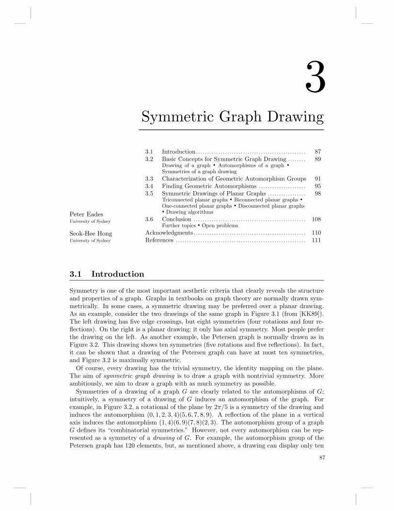
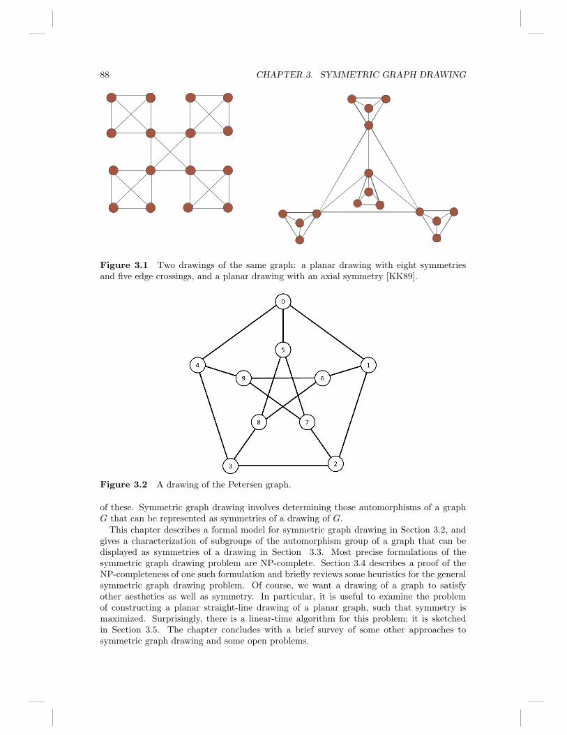
Symmetry is one of the most important aesthetic criteria that clearly reveals the structureand properties of a graph. Graphs in textbooks on graph theory are normally drawn sym-metrically. In some cases, a symmetric drawing may be preferred over a planar drawing.As an example, consider the two drawings of the same graph in Figure 3.1 (from [KK89]).The left drawing has five edge crossings, but eight symmetries (four rotations and four re-flections). On the right is a planar drawing; it only has axial symmetry. Most people preferthe drawing on the left. As another example, the Petersen graph is normally drawn as inFigure 3.2. This drawing shows ten symmetries (five rotations and five reflections). In fact,it can be shown that a drawing of the Petersen graph can have at most ten symmetries,and Figure 3.2 is maximally symmetric.

Of course, every drawing has the trivial symmetry, the identity mapping on the plane.The aim of symmetric graph drawing is to draw a graph with nontrivial symmetry. Moreambitiously, we aim to draw a graph with as much symmetry as possible.Symmetries of a drawing of a graph G are clearly related to the automorphisms of G;

intuitively, a symmetry of a drawing of G induces an automorphism of the graph. Forexample, in Figure 3.2, a rotational of the plane by 2π/5 is a symmetry of the drawing andinduces the automorphism (0, 1, 2, 3, 4)(5, 6, 7, 8, 9). A reflection of the plane in a verticalaxis induces the automorphism (1, 4)(6, 9)(7, 8)(2, 3). The automorphism group of a graphG defines its “combinatorial symmetries.” However, not every automorphism can be rep-resented as a symmetry of a drawing of G. For example, the automorphism group of thePetersen graph has 120 elements, but, as mentioned above, a drawing can display only ten

87

88 CHAPTER 3. SYMMETRIC GRAPH DRAWING

Figure 3.1 Two drawings of the same graph: a planar drawing with eight symmetriesand five edge crossings, and a planar drawing with an axial symmetry [KK89].

Figure 3.2 A drawing of the Petersen graph.

of these. Symmetric graph drawing involves determining those automorphisms of a graphG that can be represented as symmetries of a drawing of G.

This chapter describes a formal model for symmetric graph drawing in Section 3.2, andgives a characterization of subgroups of the automorphism group of a graph that can bedisplayed as symmetries of a drawing in Section 3.3. Most precise formulations of thesymmetric graph drawing problem are NP-complete. Section 3.4 describes a proof of theNP-completeness of one such formulation and briefly reviews some heuristics for the generalsymmetric graph drawing problem. Of course, we want a drawing of a graph to satisfyother aesthetics as well as symmetry. In particular, it is useful to examine the problemof constructing a planar straight-line drawing of a planar graph, such that symmetry ismaximized. Surprisingly, there is a linear-time algorithm for this problem; it is sketchedin Section 3.5. The chapter concludes with a brief survey of some other approaches tosymmetric graph drawing and some open problems.

3.2. BASIC CONCEPTS FOR SYMMETRIC GRAPH DRAWING 89

3.2 Basic Concepts for Symmetric Graph Drawing

3.2.1 Drawing of a graph

A graph G = (V,E) consists of a set V of vertices and a set E edges, that is, unorderedpairs of vertices. Unless explicitly stated otherwise, we assume that the graph is simple,that is, it has no multiple edges and no self-loops.

A drawing D of a graph G consists of a point DV (u) in R2 for every vertex u ∈ V , anda closed curve segment DE(u, v) in R2 for every edge (u, v) ∈ E. The curve DE(u, v) hasits endpoints at DV (u) and DV (v). Through most of this chapter, the curve DE(u, v) is astraight-line segment.

For an investigation of symmetric graph drawing, we must take a little care about thedefinition of the drawing of a graph. We allow two curves DE(u, v) and DE(u

′, v′) to cross(share a point), but we have some non-degeneracy conditions as follows:1

ND1 The mapping DV is injective. This excludes, for example, the ultra-symmetriccase where all vertices are drawn at the origin.

ND2 A curve DE(u, v) must not contain a point DV (w) where u 6= w 6= v; in otherwords, an edge must not intersect with a vertex to which it is not incident.

ND3 Two curves must not overlap; that is, they must not share a curve of nonzerolength. This excludes, for example, the axially symmetric case where all thevertices of the graph are drawn on the x axis.

ND4 If two curves share a point, then they must cross at this point; that is, theyalternate in cyclic order around the crossing point.

Note that for straight-line drawings, ND2 implies both ND3 and ND4. Most of this chapteris concerned with straight-line drawings, and so discussions of degeneracy concentrate onND1 and ND2.

3.2.2 Automorphisms of a graph

Basic concepts and terminology for permutation groups can be found in [Wie64].

An isomorphism from a graph G1 = (V1, E1) to a graph G2 = (V2, E2) is a one-one mapping β of V1 onto V2 that preserves adjacency, that is, (u, v) ∈ E1 if and only(β(u), β(v)) ∈ E2. An automorphism of a graph G = (V,E) is an isomorphism of G ontoitself, that is, a permutation of the vertex set that preserves adjacency. The order of anautomorphism β is the smallest positive integer k such that βk is the identity.

Any set of automorphisms of G that forms a group is called an automorphism group ofG; the set of all automorphisms of G is denoted by aut(G). The size of an automorphismgroup is the number of elements of the group.

We have defined an automorphism group A of a graph as a permutation group on thevertex set V of a graph G = (V,E). It is easy to see that this defines a permutation groupA′ acting on the edge set E, and it is often convenient to regard A as acting on E. For

1The graph drawing literature is somewhat inconsistent about the precise details of the definition ofa graph drawing. In some places, a drawing with these non-degeneracy conditions is called a strict,clear, and/or proper. In this chapter, however, we use the term “graph drawing” to includes thesenon-degeneracy conditions.


example, if β ∈ A and (u, v) ∈ E, then we write “the edge β(u, v)” to denote the edge(β(u), β(v)).

A subset B = β1, β2, . . . , βk of an automorphism group A generates A if every elementof A can be written as a product of elements of B. We denote the group A generated by B by〈β1, β2, . . . , βk〉. From the computational point of view, generators are important becausethey give a succinct way to represent an automorphism group. If we were to represent apermutation explicitly, then it may require Ω(n) space, where n = |V |. Thus, an explicitrepresentation of an automorphism group of size k may take space Ω(kn). In many casesthis is too large; for example, the space requirement may preclude a linear-time algorithm,merely because the representation of the output is super-linear. To avoid this problem, weusually represent a group by a set of generators; in general the set of generators is smallerthan the group. Most of the groups discussed in this chapter are generated by one or twoelements.

Many of the difficulties of symmetric graph drawing arise when vertices and/or edges arefixed by an automorphism. For this reason, we need a careful notion of “fix.” Suppose thatA is an automorphism group of G = (V,E). The stabilizer of u ∈ V , denoted by stabA(u),is the set of automorphisms in A that fix u, that is,

stabA(u) = β ∈ A | β(u) = u. (3.1)

The definition can be extended to subsets of V : if Y ⊆ V , then

stabA(Y ) = β ∈ A | ∀y ∈ Y, β(y) ∈ Y . (3.2)

Note that the stabilizer of a set fixes the set setwise.For each automorphism β we denote u ∈ V | β(u) = u by fixβ . The set of vertices

that are fixed elementwise by every element of A is denoted by fixA, that is,

fixA = v ∈ V | ∀ β ∈ A, β(v) = v . (3.3)

Note that while stabA(Y ) is a set of group elements, fixA is a set of vertices. Further, theexpression “fix the edge (u, v)” does not necessarily entail “fixing u and fixing v”; it couldmean that u and v are swapped.

If β ∈ A and u ∈ V , then the orbit of u under β, denoted by orbitβ(u), is the set ofimages of u under 〈β〉, that is,

orbitβ(u) = βi(u) | 0 ≤ i < k, (3.4)

where β has order k. We can extend this definition to groups: the orbit of u under A is

orbitA(u) = β(u) | β ∈ A. (3.5)

Note that the orbits partition V . The following theorem is fundamental in finite grouptheory.

Theorem 3.1 (Orbit-stabilizer theorem [Arm88]) Suppose that A is a group actingon a set X and let x ∈ X. Then |A| = |orbitA(x)| × |stabA(x)|.

The following corollary is helpful in the following sections.

COROLLARY 3.1 Suppose that A is a group acting on a set X.

• If A has no fixed points, then |orbitA(x)| = |A| for every x ∈ X.

• If A has one fixed point w ∈ X, then |orbitA(x)| = |A| for every x 6= w ∈ X.

3.3. CHARACTERIZATION OF GEOMETRIC AUTOMORPHISM GROUPS 91

3.2.3 Symmetries of a graph drawing

Symmetry is an intuitive notion that can be formally defined in many different ways. Inthis chapter we will concentrate on a standard mathematical notion of symmetry; othernotions are discussed in Section 3.6.

An isometry is a mapping of the plane onto itself that preserves distances. A symmetryof a drawing D = (DV , DE) of a graph G = (V,E) is an isometry σ of the plane that mapsthe drawing onto itself, that is:

• for every vertex u ∈ V , there is a vertex v ∈ V such that σ(DV (u)) = DV (v),and

• for every edge (u, v) ∈ E, there is an edge (a, b) ∈ E such that σ(DE(u, v)) =DE(a, b).

Note that if σ is a symmetry of a drawing D = (DV , DE) of a graph G = (V,E), thenβ = D−1

V σDV is an automorphism of G. We say that D displays β. Given an automorphismβ, if there is a drawing which displays β, then we say that β is geometric.

An automorphism group A is geometric if every element of A is displayed in a singledrawing; in this case the drawing displays A.

To define the intuitive notion of “maximally symmetric drawing” of a graph, we need todecide what it means for one drawing to display more symmetry than another. Here wetake a simple view: that if D displays A and D′ displays A′, then D is more symmetric thanD′ if A has a larger size than A′. This means that searching for a maximally symmetricdrawing entails searching for a maximum size geometric automorphism group.

3.3 Characterization of Geometric Automorphism Groups

Suppose that a drawing D of a graph G = (V,E) displays the automorphism group A. LetA′ denote the group of symmetries of D. It is useful to note the group-theoretic relationshipbetween A and A′. If D contains three non-collinear points, then A is isomorphic to A′

because a motion of three non-collinear points in the plane uniquely determines an isometry.If all the vertices of the drawing lie on a single line, it may be the case that |A′| = 4 while|A| = 2, because the rotation by π gives the same automorphism as a reflection in the line.However, this is a pathological case, because the only graphs that have drawings on a singleline are sets of paths; in general, we assume that A is isomorphic to A′.

Next, we consider the simple question: Given an automorphism group A of a graph G,is there a drawing of G that displays A? The answer is straightforward, since a symmetryof a finite set of points in the plane is relatively straightforward. The following theorem isan extension of results of Lipton et al. [LNS85], Manning et al. [MA86, MA88, AM88], andLin [Lin92] to handle degeneracies.

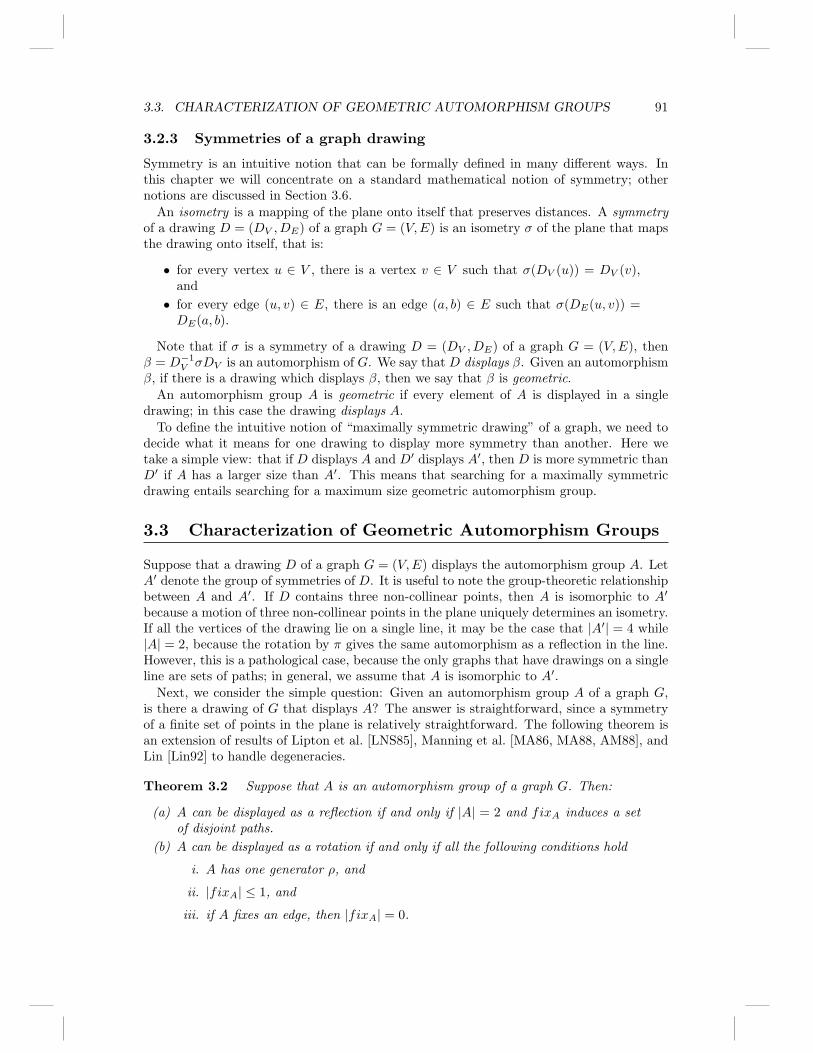
Theorem 3.2 Suppose that A is an automorphism group of a graph G. Then:

(a) A can be displayed as a reflection if and only if |A| = 2 and fixA induces a setof disjoint paths.

(b) A can be displayed as a rotation if and only if all the following conditions hold

i. A has one generator ρ, and

ii. |fixA| ≤ 1, and

iii. if A fixes an edge, then |fixA| = 0.


C 1

C 2

C 3

R 0

R 1

R 2

R 3

R 4

R 5

R 6

R 7

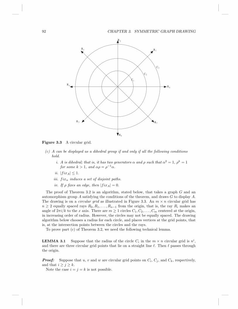
Figure 3.3 A circular grid.

(c) A can be displayed as a dihedral group if and only if all the following conditionshold.

i. A is dihedral; that is, it has two generators α and ρ such that α2 = 1, ρk = 1for some k > 1, and αρ = ρ−1α.

ii. |fixA| ≤ 1.

iii. fixα induces a set of disjoint paths.

iv. If ρ fixes an edge, then |fixA| = 0.

The proof of Theorem 3.2 is an algorithm, stated below, that takes a graph G and anautomorphism group A satisfying the conditions of the theorem, and draws G to display A.The drawing is on a circular grid as illustrated in Figure 3.3. An m × n circular grid hasn ≥ 2 equally spaced rays R0, R1, . . . , Rn−1 from the origin, that is, the ray Ri makes anangle of 2πi/k to the x axis. There are m ≥ 1 circles C1, C2, . . . , Cm centered at the origin,in increasing order of radius. However, the circles may not be equally spaced. The drawingalgorithm below chooses a radius for each circle, and places vertices at the grid points, thatis, at the intersection points between the circles and the rays.To prove part (c) of Theorem 3.2, we need the following technical lemma.

LEMMA 3.1 Suppose that the radius of the circle Ci in the m × n circular grid is ni,and there are three circular grid points that lie on a straight line ℓ. Then ℓ passes throughthe origin.

Proof: Suppose that u, v and w are circular grid points on Ci, Cj , and Ck, respectively,and that i ≥ j ≥ k.

Note the case i = j = k is not possible.

3.3. CHARACTERIZATION OF GEOMETRIC AUTOMORPHISM GROUPS 93

C j

C i

v

u

C k

O

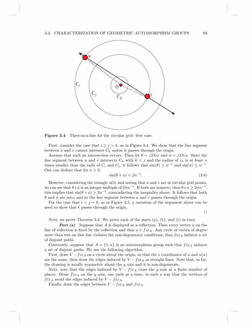
Figure 3.4 Three-in-a-line for the circular grid: first case.

First, consider the case that i ≥ j > k, as in Figure 3.4. We show that the line segmentbetween u and v cannot intersect Ck unless it passes through the origin.Assume that such an intersection occurs. Then let θ = ∠Ouv and φ = ∠Ovu. Since the

line segment between u and v intersects Ck with k < j and the radius of ck is at least ntimes smaller than the radii of Ci and Cj , it follows that sin(θ) ≤ n−1 and sin(φ) ≤ n−1.One can deduce that for n > 2:

sin(θ + φ) < 2n−1. (3.6)

However, considering the triangle uOv and noting that u and v are at circular grid points,we can see that θ+φ is an integer multiple of 2πn−1. If both are nonzero, then θ+φ ≥ 2πn−1;this implies that sin(θ+φ) ≥ 2n−1, contradicting the inequality above. It follows that bothθ and φ are zero, and so the line segment between u and v passes through the origin.

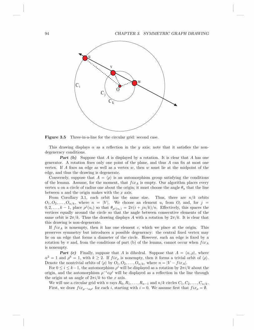
For the case that i > j = k, as in Figure 3.5, a variation of the argument above can beused to show that ℓ passes through the origin.

Next, we prove Theorem 3.2. We prove each of the parts (a), (b), and (c) in turn.

Part (a) Suppose that A is displayed as a reflection. Then every vertex u on theline of reflection is fixed by the reflection and thus u ∈ fixA. Any cycle or vertex of degreemore than two on this line violates the non-degeneracy conditions, thus fixA induces a setof disjoint paths.

Conversely, suppose that A = 1, α is an automorphism group such that fixA inducesa set of disjoint paths. We use the following algorithm.

First, draw V −fixA on a circle about the origin, so that the x coordinates of u and α(u)are the same, then draw the edges induced by V − fixA as straight lines. Note that, so far,the drawing is axially symmetric about the y axis and it is non-degenerate.

Next, note that the edges induced by V − fixA cross the y axis at a finite number ofplaces. Draw fixA on the y axis, one path at a time, in such a way that the vertices offixA avoid the edges induced by V − fixA.

Finally, draw the edges between V − fixA and fixA.


C j

C i

v

u

C k

w

O

Figure 3.5 Three-in-a-line for the circular grid: second case.

This drawing displays α as a reflection in the y axis; note that it satisfies the non-degeneracy conditions.

Part (b) Suppose that A is displayed by a rotation. It is clear that A has onegenerator. A rotation fixes only one point of the plane, and thus A can fix at most onevertex. If A fixes an edge as well as a vertex w, then w must lie at the midpoint of theedge, and thus the drawing is degenerate.

Conversely, suppose that A = 〈ρ〉 is an automorphism group satisfying the conditionsof the lemma. Assume, for the moment, that fixA is empty. Our algorithm places everyvertex u on a circle of radius one about the origin; it must choose the angle θu that the linebetween u and the origin makes with the x axis.

From Corollary 3.1, each orbit has the same size. Thus, there are n/k orbitsO1, O2, . . . , On/k, where n = |V |. We choose an element ui from Oi and, for j =0, 2, . . . , k − 1, place ρj(ui) so that θρj(ui) = 2π(i + jn/k)/n. Effectively, this spaces thevertices equally around the circle so that the angle between consecutive elements of thesame orbit is 2π/k. Thus the drawing displays A with a rotation by 2π/k. It is clear thatthis drawing is non-degenerate.

If fixA is nonempty, then it has one element c, which we place at the origin. Thispreserves symmetry but introduces a possible degeneracy: the central fixed vertex maylie on an edge that forms a diameter of the circle. However, such an edge is fixed by arotation by π and, from the conditions of part (b) of the lemma, cannot occur when fixA

is nonempty.

Part (c) Finally, suppose that A is dihedral. Suppose that A = 〈α, ρ〉, whereα2 = 1 and ρk = 1, with k ≥ 2. If fixρ is nonempty, then it forms a trivial orbit of 〈ρ〉.Denote the nontrivial orbits of 〈ρ〉 by O1, O2, . . . , On/k, where n = |V − fixA|.

For 0 ≤ i ≤ k−1, the automorphism ρi will be displayed as a rotation by 2πi/k about theorigin, and the automorphism ρ−iαρi will be displayed as a reflection in the line throughthe origin at an angle of 2πi/k to the x axis.

We will use a circular grid with n rays R0, R1, . . . , Rn−1 and n/k circles C1, C2, . . . , Cn/k.First, we draw fixρ−iαρi for each i, starting with i = 0. We assume first that fixρ = ∅.

3.4. FINDING GEOMETRIC AUTOMORPHISMS 95

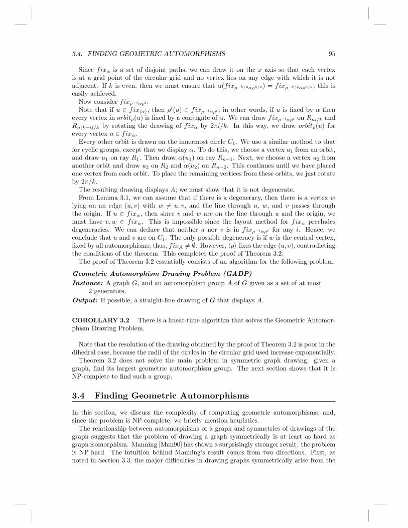
Since fixα is a set of disjoint paths, we can draw it on the x axis so that each vertexis at a grid point of the circular grid and no vertex lies on any edge with which it is notadjacent. If k is even, then we must ensure that α(fixρ−k/2αρk/2) = fixρ−k/2αρk/2 ; this iseasily achieved.

Now consider fixρ−iαρi .Note that if u ∈ fix〈α〉, then ρi(u) ∈ fixρ−iαρi ; in other words, if u is fixed by α then

every vertex in orbitρ(u) is fixed by a conjugate of α. We can draw fixρ−iαρi on Rni/k andRn(k−i)/k by rotating the drawing of fixα by 2πi/k. In this way, we draw orbitρ(u) forevery vertex u ∈ fixα.

Every other orbit is drawn on the innermost circle C1. We use a similar method to thatfor cyclic groups, except that we display α. To do this, we choose a vertex u1 from an orbit,and draw u1 on ray R1. Then draw α(u1) on ray Rn−1. Next, we choose a vertex u2 fromanother orbit and draw u2 on R2 and α(u2) on Rn−2. This continues until we have placedone vertex from each orbit. To place the remaining vertices from these orbits, we just rotateby 2π/k.

The resulting drawing displays A; we must show that it is not degenerate.From Lemma 3.1, we can assume that if there is a degeneracy, then there is a vertex w

lying on an edge (u, v) with w 6= u, v, and the line through u, w, and v passes throughthe origin. If u ∈ fixα, then since v and w are on the line through u and the origin, wemust have v, w ∈ fixα. This is impossible since the layout method for fixα precludesdegeneracies. We can deduce that neither u nor v is in fixρ−iαρi for any i. Hence, weconclude that u and v are on C1. The only possible degeneracy is if w is the central vertex,fixed by all automorphisms; thus, fixA 6= ∅. However, 〈ρ〉 fixes the edge (u, v), contradictingthe conditions of the theorem. This completes the proof of Theorem 3.2.

The proof of Theorem 3.2 essentially consists of an algorithm for the following problem.

Geometric Automorphism Drawing Problem (GADP)

Instance: A graph G, and an automorphism group A of G given as a set of at most2 generators.

Output: If possible, a straight-line drawing of G that displays A.

COROLLARY 3.2 There is a linear-time algorithm that solves the Geometric Automor-phism Drawing Problem.

Note that the resolution of the drawing obtained by the proof of Theorem 3.2 is poor in thedihedral case, because the radii of the circles in the circular grid used increase exponentially.

Theorem 3.2 does not solve the main problem in symmetric graph drawing: given agraph, find its largest geometric automorphism group. The next section shows that it isNP-complete to find such a group.

3.4 Finding Geometric Automorphisms

In this section, we discuss the complexity of computing geometric automorphisms, and,since the problem is NP-complete, we briefly mention heuristics.

The relationship between automorphisms of a graph and symmetries of drawings of thegraph suggests that the problem of drawing a graph symmetrically is at least as hard asgraph isomorphism. Manning [Man90] has shown a surprisingly stronger result: the problemis NP-hard. The intuition behind Manning’s result comes from two directions. First, asnoted in Section 3.3, the major difficulties in drawing graphs symmetrically arise from the


u 1

u 2

u 3

u 4

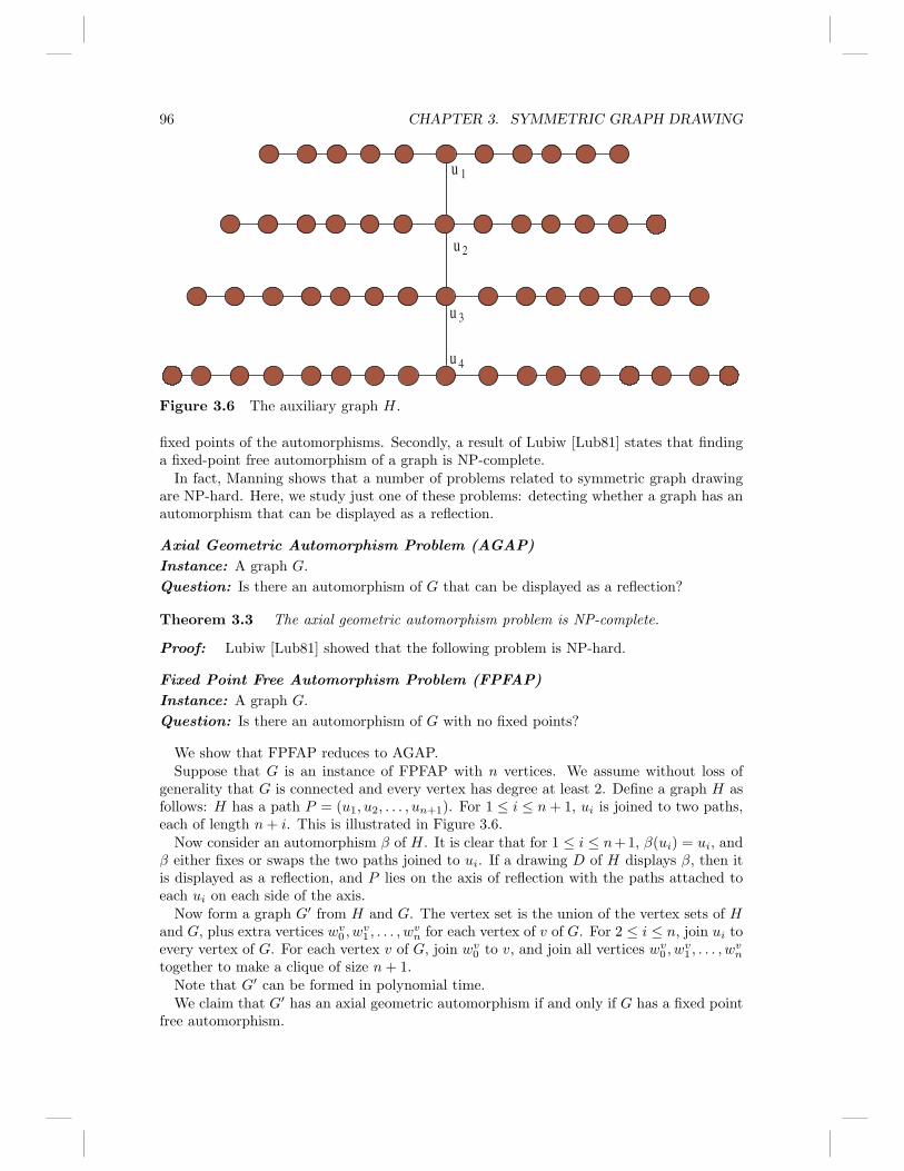
Figure 3.6 The auxiliary graph H.

fixed points of the automorphisms. Secondly, a result of Lubiw [Lub81] states that findinga fixed-point free automorphism of a graph is NP-complete.

In fact, Manning shows that a number of problems related to symmetric graph drawingare NP-hard. Here, we study just one of these problems: detecting whether a graph has anautomorphism that can be displayed as a reflection.

Axial Geometric Automorphism Problem (AGAP)

Instance: A graph G.

Question: Is there an automorphism of G that can be displayed as a reflection?

Theorem 3.3 The axial geometric automorphism problem is NP-complete.

Proof: Lubiw [Lub81] showed that the following problem is NP-hard.

Fixed Point Free Automorphism Problem (FPFAP)

Instance: A graph G.

Question: Is there an automorphism of G with no fixed points?

We show that FPFAP reduces to AGAP.Suppose that G is an instance of FPFAP with n vertices. We assume without loss of

generality that G is connected and every vertex has degree at least 2. Define a graph H asfollows: H has a path P = (u1, u2, . . . , un+1). For 1 ≤ i ≤ n+ 1, ui is joined to two paths,each of length n+ i. This is illustrated in Figure 3.6.

Now consider an automorphism β of H. It is clear that for 1 ≤ i ≤ n+1, β(ui) = ui, andβ either fixes or swaps the two paths joined to ui. If a drawing D of H displays β, then itis displayed as a reflection, and P lies on the axis of reflection with the paths attached toeach ui on each side of the axis.

Now form a graph G′ from H and G. The vertex set is the union of the vertex sets of Hand G, plus extra vertices wv

0 , wv1 , . . . , w

vn for each vertex of v of G. For 2 ≤ i ≤ n, join ui to

every vertex of G. For each vertex v of G, join wv0 to v, and join all vertices wv

0 , wv1 , . . . , w

vn

together to make a clique of size n+ 1.Note that G′ can be formed in polynomial time.We claim that G′ has an axial geometric automorphism if and only if G has a fixed point

free automorphism.

3.4. FINDING GEOMETRIC AUTOMORPHISMS 97

First, suppose that G has a fixed point free automorphism β. It is clear that one canextend β to G′ to give an automorphism that satisfies part (a) of Theorem 3.2, and so G′

has an axial geometric automorphism group.Now suppose that G′ has an axial geometric automorphism γ.We claim that γ cannot map a vertex w of H to a vertex v of G, or to one of the new

vertices wvi . This is because every vertex of G is adjacent to a clique of size n + 1, while

no vertex of H has this property. Further, γ cannot map a vertex of G to one of the newvertices wv

i , because each wvi is in a clique of size n + 1, and none of the original vertices

have this property. Thus, γ restricted to H is an automorphism β of H; as mentionedabove, the only drawing that displays β has P lying on the axis of reflection.Also, γ restricted to G is an automorphism δ of G. Suppose that δ has a fixed point v.

Recall that v is joined by an edge to a vertex ui in P ; this means that the induced subgraphfixγ has a vertex of degree at least three. From Theorem 3.2, this is impossible. Thus δ isfixed-point-free.

Finally, note that AGAP is in NP, because one can guess an automorphism group, and,using Theorem 3.2, check whether it is geometric.

The NP-completeness results have led to a number of heuristic approaches; see [dF99,Kam89, Lin92, LNS85].

The most common are the generic multidimensional scaling, or force directed meth-ods [dF99, Ead84, Kam88, Lin92]. Roughly speaking, this method projects a high-dimensional drawing of the graph into low dimensions. The first step is to define a dis-tance function d between vertices, and then the graph is drawn in a high-dimensional spacein such a way that the Euclidean distance in the high-dimensional space is equal or closeto the distances defined by d. In some cases, this (high-dimensional) drawing is uniqueup to isometry; this implies that every automorphism of the graph is a symmetry of thedrawing. In other words, it achieves maximum symmetry in the high dimension. The nextstep is to project the high-dimensional drawing into a low-dimensional space (either 2 or 3dimensions) in such a way that the distances are preserved as much as possible.As an example of such a method, de Fraysseix [dF99] uses the Czekanovski-Dice semi-

distance for a graph G = (V,E):

d(u, v) =

√

1− 2|Nu ∩Nv|

|Nu|+ |Nv|. (3.7)

(A semi-distance d : X → R is a function that is almost a distance function: it satisfiestwo of the axioms of a distance function: d(u, v) = d(v, u) and d(u, v) + d(v, w) ≥ d(u,w).However, it is possible that there are distinct elements u, v ∈ X with d(u, v) = 0.) DeFraysseix uses projections defined by the principal components of the corresponding innerproduct matrix whose entries are defined by a pair s, t of vertices as follows:

Wst =1

2(d2s + d2t − d2V ), (3.8)

where for w = s, t,

d2w =1

n

∑

u∈V

d2(w, u), (3.9)

and

d2V =1

n

∑

w∈V

d2w. (3.10)


These projections are remarkably successful in displaying two dimensional symmetry;see [dF99] for details.

It is common to look at such methods as a system of forces: for example, one can simulatea system of forces between vertices where the force exerted on u by v is proportional to thedistance d(u, v). A minimum energy configuration defines a drawing, and in many casesthis drawing displays symmetries. For example, one can view the Tutte method [Tut63,DETT99] in this way. In fact, one of the reasons for the popularity of force directed methodsis the fact that the drawings often display some symmetry. One can give some explanation(see [EL00, Lin92]) of why the approach works.

3.5 Symmetric Drawings of Planar Graphs

In this section, we describe a linear-time algorithm to draw planar graphs with no edgecrossings and as much symmetry as possible.

The concept of geometric automorphism in Section 3.2.3 can be extended to planar draw-ings: an automorphism β of a graph G is planar if there is a planar drawing of G thatdisplays β, and an automorphism group A is a planar automorphism group if there is aplanar drawing which displays every element of A.The problem of finding automorphisms of a planar graph can be solved in linear time

(see [HW74, Won75]); however, it is clear that not all automorphisms are geometric. Fur-ther, not every geometric automorphism is planar. For example, the complete graph K4

with four vertices has a dihedral geometric automorphism group of size eight, but this groupis not planar. The largest planar automorphism group of K4 has size six.The following theorem summarizes the result.

Theorem 3.4 There is a linear-time algorithm that constructs maximum planar auto-morphism group of a planar graph.

The remainder of this section is a sketch of a proof of Theorem 3.4. The algorithmto prove the theorem uses a connectivity decomposition. We decompose the graph intoconnected components, then decompose each connected component into biconnected com-ponents, and finally decompose each biconnected component into triconnected components.Different algorithms are needed for triconnected, biconnected, one-connected, and discon-nected graphs. Each uses the algorithms for higher connectivity as subroutines. Details ofthe proof can be found in [HE05, HE06, HE03, HME06].

In Section 3.5.5, we briefly describe the drawing algorithms.

3.5.1 Triconnected planar graphs

This section describes an algorithm for finding planar automorphism groups of maximumsize for triconnected planar graphs.

The uniqueness of the faces of a triconnected planar graph G = (V,E) means that anautomorphism group A defines a permutation group acting on the set F of faces of G.Effectively this means that A defines an automorphism group of the dual G∗ of G. We canregard A as acting on G∗, and write, for example, “the face β(f)” for some β ∈ A, f ∈ F .

It is well known that a triconnected planar graph can be represented as the skeleton ofa polyhedron in three dimensions [SR34]. A more surprising and less well known result,due to Mani [Bab95, Man71], states that the automorphism group of a triconnected planargraph can be completely encapsulated in the symmetries of a polyhedron. The symmetryfinding algorithm relies on this fundamental result.

3.5. SYMMETRIC DRAWINGS OF PLANAR GRAPHS 99

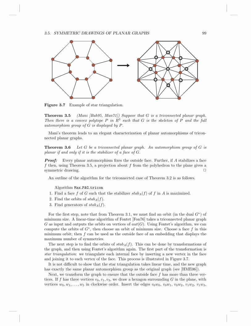
Figure 3.7 Example of star triangulation.

Theorem 3.5 (Mani [Bab95, Man71]) Suppose that G is a triconnected planar graph.Then there is a convex polytope P in R3 such that G is the skeleton of P and the fullautomorphism group of G is displayed by P .

Mani’s theorem leads to an elegant characterization of planar automorphisms of tricon-nected planar graphs.

Theorem 3.6 Let G be a triconnected planar graph. An automorphism group of G isplanar if and only if it is the stabilizer of a face of G.

Proof: Every planar automorphism fixes the outside face. Further, if A stabilizes a facef then, using Theorem 3.5, a projection about f from the polyhedron to the plane gives asymmetric drawing.

An outline of the algorithm for the triconnected case of Theorem 3.2 is as follows.

Algorithm Max PAG tricon

1. Find a face f of G such that the stabilizer stabA(f) of f in A is maximized.

2. Find the orbits of stabA(f).

3. Find generators of stabA(f).

For the first step, note that from Theorem 3.1, we must find an orbit (in the dual G∗) ofminimum size. A linear-time algorithm of Fontet [Fon76] takes a triconnected planar graphG as input and outputs the orbits on vertices of aut(G). Using Fontet’s algorithm, we cancompute the orbits of G∗, then choose an orbit of minimum size. Choose a face f in thisminimum orbit; then f can be used as the outside face of an embedding that displays themaximum number of symmetries.

The next step is to find the orbits of stabA(f). This can be done by transformations ofthe graph, and then using Fontet’s algorithm again. The first part of the transformation isstar triangulation: we triangulate each internal face by inserting a new vertex in the faceand joining it to each vertex of the face. This process is illustrated in Figure 3.7.

It is not difficult to show that the star triangulation takes linear time, and the new graphhas exactly the same planar automorphism group as the original graph (see [HME06]).

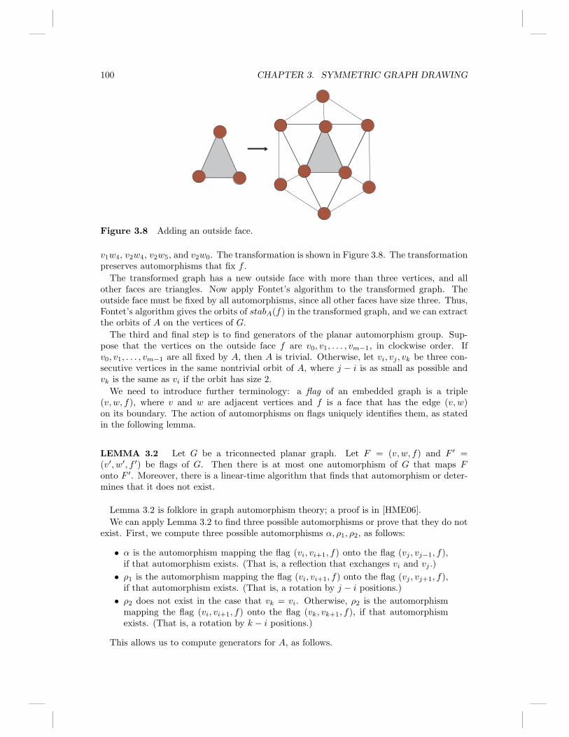
Next, we transform the graph to ensure that the outside face f has more than three ver-tices. If f has three vertices v0, v1, v3, we draw a hexagon surrounding G in the plane, withvertices w0, w1, . . . , w5 in clockwise order. Insert the edges v0w0, v0w1, v0w2, v1w2, v1w3,


Figure 3.8 Adding an outside face.

v1w4, v2w4, v2w5, and v2w0. The transformation is shown in Figure 3.8. The transformationpreserves automorphisms that fix f .

The transformed graph has a new outside face with more than three vertices, and allother faces are triangles. Now apply Fontet’s algorithm to the transformed graph. Theoutside face must be fixed by all automorphisms, since all other faces have size three. Thus,Fontet’s algorithm gives the orbits of stabA(f) in the transformed graph, and we can extractthe orbits of A on the vertices of G.

The third and final step is to find generators of the planar automorphism group. Sup-pose that the vertices on the outside face f are v0, v1, . . . , vm−1, in clockwise order. Ifv0, v1, . . . , vm−1 are all fixed by A, then A is trivial. Otherwise, let vi, vj , vk be three con-secutive vertices in the same nontrivial orbit of A, where j − i is as small as possible andvk is the same as vi if the orbit has size 2.

We need to introduce further terminology: a flag of an embedded graph is a triple(v, w, f), where v and w are adjacent vertices and f is a face that has the edge (v, w)on its boundary. The action of automorphisms on flags uniquely identifies them, as statedin the following lemma.

LEMMA 3.2 Let G be a triconnected planar graph. Let F = (v, w, f) and F ′ =(v′, w′, f ′) be flags of G. Then there is at most one automorphism of G that maps Fonto F ′. Moreover, there is a linear-time algorithm that finds that automorphism or deter-mines that it does not exist.

Lemma 3.2 is folklore in graph automorphism theory; a proof is in [HME06].

We can apply Lemma 3.2 to find three possible automorphisms or prove that they do notexist. First, we compute three possible automorphisms α, ρ1, ρ2, as follows:

• α is the automorphism mapping the flag (vi, vi+1, f) onto the flag (vj , vj−1, f),if that automorphism exists. (That is, a reflection that exchanges vi and vj .)

• ρ1 is the automorphism mapping the flag (vi, vi+1, f) onto the flag (vj , vj+1, f),if that automorphism exists. (That is, a rotation by j − i positions.)

• ρ2 does not exist in the case that vk = vi. Otherwise, ρ2 is the automorphismmapping the flag (vi, vi+1, f) onto the flag (vk, vk+1, f), if that automorphismexists. (That is, a rotation by k − i positions.)

This allows us to compute generators for A, as follows.


• If α does not exist, then ρ1 exists and A is a cyclic group of size m/(j − i)generated by the rotation ρ1.

• If α exists but neither ρ1 nor ρ2 exists, then A is the group of size 2 generatedby the reflection α.

• If α and ρ1 exist, then A is the dihedral group of size 2m/(j − i) generated bythe reflection α and the rotation ρ1.

• Otherwise, α and ρ2 exist, and A is the dihedral group of size 2m/(k−i) generatedby the reflection α and the rotation ρ2.

We summarize this section with the following lemma.

LEMMA 3.3 Algorithm Max PAG tricon computes generators for the largest planarautomorphism group of a triconnected planar graph in linear time.

3.5.2 Biconnected planar graphs

If the input graph G is biconnected, then we break it into triconnected components andapply the algorithm for triconnected graphs in Section 3.5.1. However, this process is notas simple as it sounds.

We use a version of the “SPQR-tree” to represent the decomposition of a biconnectedplanar graph into triconnected components. Various versions of the SPQR tree appear in theliterature; the version that we use is closely related to the original version of Tutte [Tut66].

It is useful to review the definition of triconnected components [HT73]. If G is tricon-nected, then G itself is the unique triconnected component of G. Otherwise, let u, v be aseparation pair of G. We split the edges of G into two disjoint subsets E1 and E2, such that|E1| > 1, |E2| > 1, and the subgraphs G1 and G2 induced by E1 and E2 only have verticesu and v in common. Form the graph G′

1 by adding an edge (called a virtual edge) between uand v; similarly, form G′

2. We continue the splitting process recursively on G′1 and G′

2. Theprocess stops when each resulting graph reaches one of three forms: a triconnected simplegraph, a set of three multiple edges (a triple bond), or a cycle of length three (a triangle).The triconnected components of G are obtained from these resulting graphs. They may beof three types:

1. a triconnected simple graph;

2. a bond, formed by merging the triple bonds into a maximal set of multiple edges;

3. a polygon, formed by merging the triangles into a maximal simple cycle.

The triconnected components of G are unique. See [HT73] for further details.Now we can describe the SPQR tree. Each node v in the SPQR tree is associated with a

graph skeleton(v), corresponding to a triconnected component. There are several types ofnodes in the SPQR tree, corresponding to the type of triconnected components describedabove. The edges of the SPQR tree are defined by the virtual edges, that is, if u and v aretwo nodes whose skeletons share a virtual edge, then u and v are connected in the SPQRtree.

The SPQR tree can be rooted at its center (if the tree has two centers, it can be rooted ateither one). The motivation for using the rooted version is that the SPQR tree is unique foreach biconnected planar graph [Bab95, DT92]. This means that the triconnected componentcorresponding to the root of the SPQR-tree is fixed by a planar automorphism group of abiconnected planar graph. Further, each leaf is mapped to a leaf. These two properties ofthe rooted SPQR tree are essential for our algorithm outlined below.


To state the algorithm, we need some more terminology. We say that a virtual edge e ofskeleton(v) is a parent (child) virtual edge if e corresponds to a virtual edge of u which isa parent (resp. child) node of v. We define a parent separation pair s = (s1, s2) of v as thetwo endpoints of a parent virtual edge e.

The overall algorithm is composed of three steps.

Algorithm MAX PAG bicon

Step 1. Construct the SPQR-tree T of G.

Step 2. Reduction: For each level i of T (from the lowest level to the root level)

(a) For each leaf node on level i, compute labels on the parent virtual edge inthe leaf node.

(b) For each leaf node on level i, label the corresponding virtual edge in theparent node with the labels.

(c) Remove the leaf nodes on level i.

Step 3. Compute a maximum size planar automorphism group at the labeled center.

We briefly describe each step of the algorithm. The first step is to construct the SPQR-treefor the input biconnected planar graph. This can be done in linear time using the classicalHopcroft-Tarjan algorithm [HT73].

The second step, reduction, is the most important. This takes the rooted SPQR-tree of abiconnected graph, and proceeds up the SPQR-tree from the leaf nodes to the center levelby level, computing labels. The labels consist of integer and boolean values that capturesome information of the planar automorphisms of the leaf nodes. First, it computes thelabels for the leaf nodes. Then, it labels the corresponding virtual edge in the parent nodeand delete each leaf node. The reduction process stops when it reaches the root.

The reduction process clearly does not decrease the planar automorphism group of theoriginal graph. This is not enough; we need to also ensure that the planar automorphismgroup is not increased by reduction. This is the role of the labels. As a leaf v is deleted, thealgorithm labels the virtual edge e of v in skeleton(u) where u is a parent of v. Roughlyspeaking, the labels encode enough information about the deleted leaf to ensure that planarautomorphisms of the labeled reduced graph can be extended to a planar automorphismsof the original graph.

We illustrate the basic idea of the algorithm with an example.

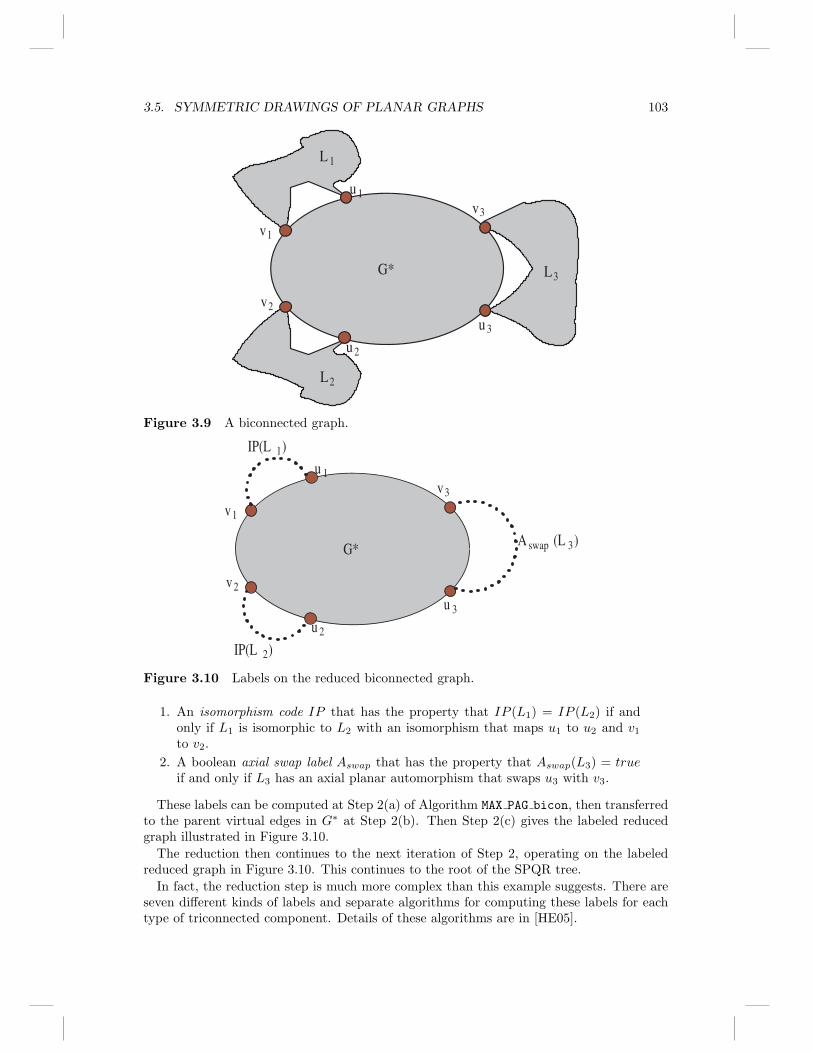
Consider the biconnected graph represented in Figure 3.9. Here the graph G has an SPQRtree with three leaves; these are triconnected components, G1, G2, and G3, illustrated byshaded blobs. The remainder of the graph, G∗, is illustrated by a shaded oval. This isconnected to the leaves by separation pairs ui, vi, for i = 1, 2, 3..

Intuitively, G can be drawn with an axial symmetry (a reflection in a horizontal line) aslong as:

1. L1 is isomorphic to L2 with an isomorphism that maps u1 to u2 and v1 to v2.

2. L3 has an axial planar automorphism that swaps u3 with v3.

3. G∗ has an axial planar automorphism that swaps u3 with v3, and maps u1 to u2

and v1 to v2.

To decide whether G can be drawn with an axial symmetry, we maintain a number oflabels, including:


G*

L 1

L 2

L 3

v 1

u 1

v 2

u 2

v 3

u 3

Figure 3.9 A biconnected graph.

G*

v 1

u 1

v 2

u 2

v 3

u 3

IP(L 1 )

IP(L 2 )

A swap (L 3 )

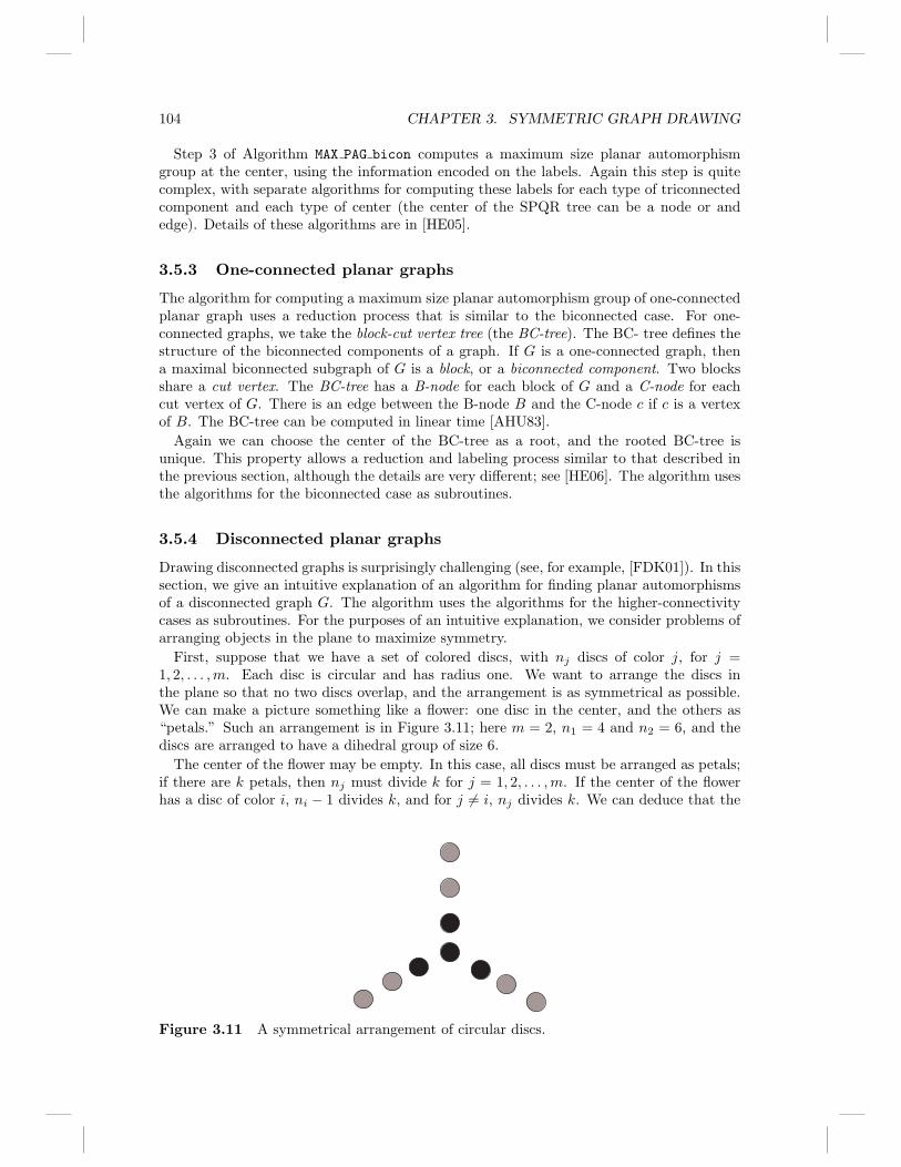
Figure 3.10 Labels on the reduced biconnected graph.

1. An isomorphism code IP that has the property that IP (L1) = IP (L2) if andonly if L1 is isomorphic to L2 with an isomorphism that maps u1 to u2 and v1to v2.

2. A boolean axial swap label Aswap that has the property that Aswap(L3) = trueif and only if L3 has an axial planar automorphism that swaps u3 with v3.

These labels can be computed at Step 2(a) of Algorithm MAX PAG bicon, then transferredto the parent virtual edges in G∗ at Step 2(b). Then Step 2(c) gives the labeled reducedgraph illustrated in Figure 3.10.

The reduction then continues to the next iteration of Step 2, operating on the labeledreduced graph in Figure 3.10. This continues to the root of the SPQR tree.

In fact, the reduction step is much more complex than this example suggests. There areseven different kinds of labels and separate algorithms for computing these labels for eachtype of triconnected component. Details of these algorithms are in [HE05].


Step 3 of Algorithm MAX PAG bicon computes a maximum size planar automorphismgroup at the center, using the information encoded on the labels. Again this step is quitecomplex, with separate algorithms for computing these labels for each type of triconnectedcomponent and each type of center (the center of the SPQR tree can be a node or andedge). Details of these algorithms are in [HE05].

3.5.3 One-connected planar graphs

The algorithm for computing a maximum size planar automorphism group of one-connectedplanar graph uses a reduction process that is similar to the biconnected case. For one-connected graphs, we take the block-cut vertex tree (the BC-tree). The BC- tree defines thestructure of the biconnected components of a graph. If G is a one-connected graph, thena maximal biconnected subgraph of G is a block, or a biconnected component. Two blocksshare a cut vertex. The BC-tree has a B-node for each block of G and a C-node for eachcut vertex of G. There is an edge between the B-node B and the C-node c if c is a vertexof B. The BC-tree can be computed in linear time [AHU83].

Again we can choose the center of the BC-tree as a root, and the rooted BC-tree isunique. This property allows a reduction and labeling process similar to that described inthe previous section, although the details are very different; see [HE06]. The algorithm usesthe algorithms for the biconnected case as subroutines.

3.5.4 Disconnected planar graphs

Drawing disconnected graphs is surprisingly challenging (see, for example, [FDK01]). In thissection, we give an intuitive explanation of an algorithm for finding planar automorphismsof a disconnected graph G. The algorithm uses the algorithms for the higher-connectivitycases as subroutines. For the purposes of an intuitive explanation, we consider problems ofarranging objects in the plane to maximize symmetry.

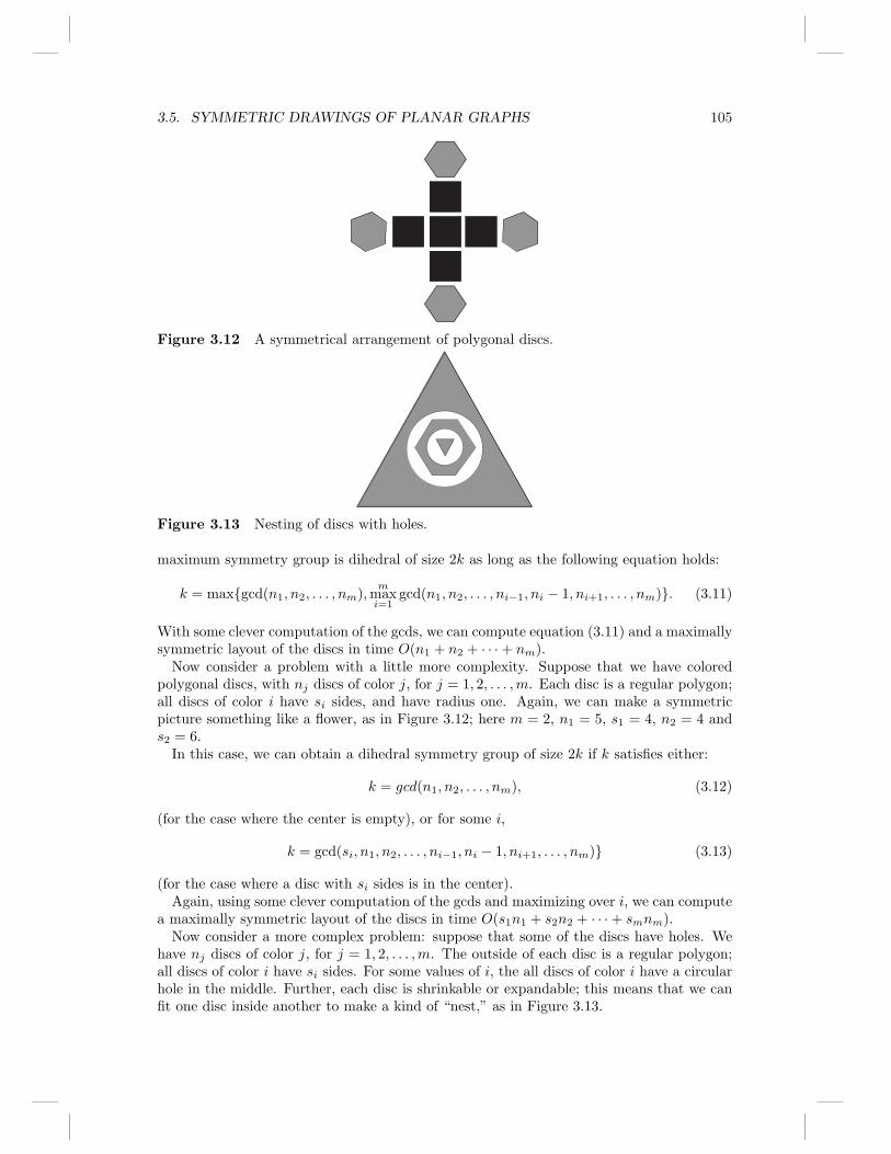
First, suppose that we have a set of colored discs, with nj discs of color j, for j =1, 2, . . . ,m. Each disc is circular and has radius one. We want to arrange the discs inthe plane so that no two discs overlap, and the arrangement is as symmetrical as possible.We can make a picture something like a flower: one disc in the center, and the others as“petals.” Such an arrangement is in Figure 3.11; here m = 2, n1 = 4 and n2 = 6, and thediscs are arranged to have a dihedral group of size 6.

The center of the flower may be empty. In this case, all discs must be arranged as petals;if there are k petals, then nj must divide k for j = 1, 2, . . . ,m. If the center of the flowerhas a disc of color i, ni − 1 divides k, and for j 6= i, nj divides k. We can deduce that the

Figure 3.11 A symmetrical arrangement of circular discs.


Figure 3.12 A symmetrical arrangement of polygonal discs.

Figure 3.13 Nesting of discs with holes.

maximum symmetry group is dihedral of size 2k as long as the following equation holds:

k = maxgcd(n1, n2, . . . , nm),m

maxi=1

gcd(n1, n2, . . . , ni−1, ni − 1, ni+1, . . . , nm). (3.11)

With some clever computation of the gcds, we can compute equation (3.11) and a maximallysymmetric layout of the discs in time O(n1 + n2 + · · ·+ nm).

Now consider a problem with a little more complexity. Suppose that we have coloredpolygonal discs, with nj discs of color j, for j = 1, 2, . . . ,m. Each disc is a regular polygon;all discs of color i have si sides, and have radius one. Again, we can make a symmetricpicture something like a flower, as in Figure 3.12; here m = 2, n1 = 5, s1 = 4, n2 = 4 ands2 = 6.

In this case, we can obtain a dihedral symmetry group of size 2k if k satisfies either:

k = gcd(n1, n2, . . . , nm), (3.12)

(for the case where the center is empty), or for some i,

k = gcd(si, n1, n2, . . . , ni−1, ni − 1, ni+1, . . . , nm) (3.13)

(for the case where a disc with si sides is in the center).Again, using some clever computation of the gcds and maximizing over i, we can compute

a maximally symmetric layout of the discs in time O(s1n1 + s2n2 + · · ·+ smnm).Now consider a more complex problem: suppose that some of the discs have holes. We

have nj discs of color j, for j = 1, 2, . . . ,m. The outside of each disc is a regular polygon;all discs of color i have si sides. For some values of i, the all discs of color i have a circularhole in the middle. Further, each disc is shrinkable or expandable; this means that we canfit one disc inside another to make a kind of “nest,” as in Figure 3.13.


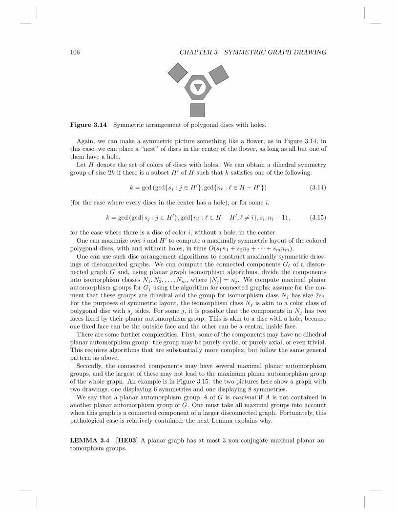
Figure 3.14 Symmetric arrangement of polygonal discs with holes.

Again, we can make a symmetric picture something like a flower, as in Figure 3.14; inthis case, we can place a “nest” of discs in the center of the flower, as long as all but one ofthem have a hole.

Let H denote the set of colors of discs with holes. We can obtain a dihedral symmetrygroup of size 2k if there is a subset H ′ of H such that k satisfies one of the following:

k = gcd (gcdsj : j ∈ H ′, gcdnℓ : ℓ ∈ H −H ′) (3.14)

(for the case where every discs in the center has a hole), or for some i,

k = gcd (gcdsj : j ∈ H ′, gcdnℓ : ℓ ∈ H −H ′, ℓ 6= i, si, ni − 1) , (3.15)

for the case where there is a disc of color i, without a hole, in the center.

One can maximize over i and H ′ to compute a maximally symmetric layout of the coloredpolygonal discs, with and without holes, in time O(s1n1 + s2n2 + · · ·+ smnm).

One can use such disc arrangement algorithms to construct maximally symmetric draw-ings of disconnected graphs. We can compute the connected components Gℓ of a discon-nected graph G and, using planar graph isomorphism algorithms, divide the componentsinto isomorphism classes N1, N2, . . . , Nm, where |Nj | = nj . We compute maximal planarautomorphism groups for Gj using the algorithm for connected graphs; assume for the mo-ment that these groups are dihedral and the group for isomorphism class Nj has size 2sj .For the purposes of symmetric layout, the isomorphism class Nj is akin to a color class ofpolygonal disc with sj sides. For some j, it is possible that the components in Nj has twofaces fixed by their planar automorphism group. This is akin to a disc with a hole, becauseone fixed face can be the outside face and the other can be a central inside face.

There are some further complexities. First, some of the components may have no dihedralplanar automorphism group: the group may be purely cyclic, or purely axial, or even trivial.This requires algorithms that are substantially more complex, but follow the same generalpattern as above.

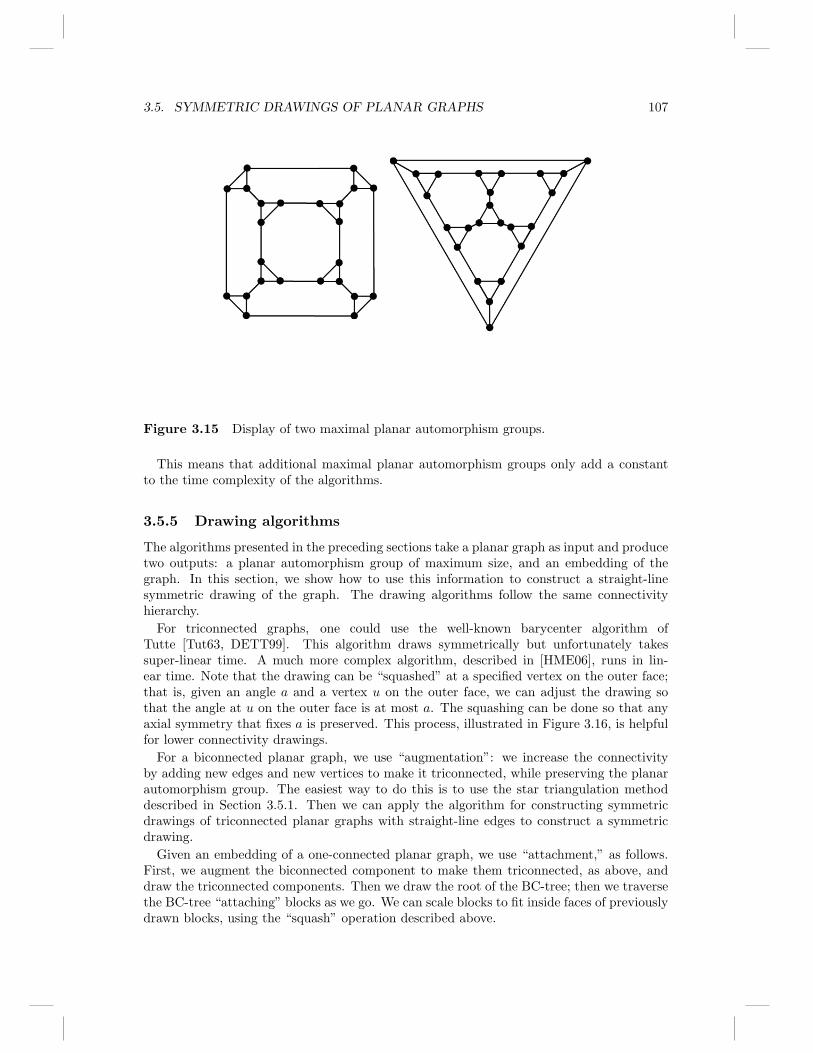
Secondly, the connected components may have several maximal planar automorphismgroups, and the largest of these may not lead to the maximum planar automorphism groupof the whole graph. An example is in Figure 3.15: the two pictures here show a graph withtwo drawings, one displaying 6 symmetries and one displaying 8 symmetries.

We say that a planar automorphism group A of G is maximal if A is not contained inanother planar automorphism group of G. One must take all maximal groups into accountwhen this graph is a connected component of a larger disconnected graph. Fortunately, thispathological case is relatively contained; the next Lemma explains why.

LEMMA 3.4 [HE03] A planar graph has at most 3 non-conjugate maximal planar au-tomorphism groups.


Figure 3.15 Display of two maximal planar automorphism groups.

This means that additional maximal planar automorphism groups only add a constantto the time complexity of the algorithms.

3.5.5 Drawing algorithms

The algorithms presented in the preceding sections take a planar graph as input and producetwo outputs: a planar automorphism group of maximum size, and an embedding of thegraph. In this section, we show how to use this information to construct a straight-linesymmetric drawing of the graph. The drawing algorithms follow the same connectivityhierarchy.

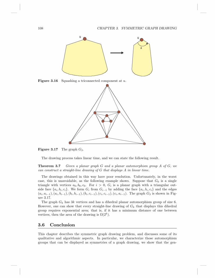
For triconnected graphs, one could use the well-known barycenter algorithm ofTutte [Tut63, DETT99]. This algorithm draws symmetrically but unfortunately takessuper-linear time. A much more complex algorithm, described in [HME06], runs in lin-ear time. Note that the drawing can be “squashed” at a specified vertex on the outer face;that is, given an angle a and a vertex u on the outer face, we can adjust the drawing sothat the angle at u on the outer face is at most a. The squashing can be done so that anyaxial symmetry that fixes a is preserved. This process, illustrated in Figure 3.16, is helpfulfor lower connectivity drawings.

For a biconnected planar graph, we use “augmentation”: we increase the connectivityby adding new edges and new vertices to make it triconnected, while preserving the planarautomorphism group. The easiest way to do this is to use the star triangulation methoddescribed in Section 3.5.1. Then we can apply the algorithm for constructing symmetricdrawings of triconnected planar graphs with straight-line edges to construct a symmetricdrawing.

Given an embedding of a one-connected planar graph, we use “attachment,” as follows.First, we augment the biconnected component to make them triconnected, as above, anddraw the triconnected components. Then we draw the root of the BC-tree; then we traversethe BC-tree “attaching” blocks as we go. We can scale blocks to fit inside faces of previouslydrawn blocks, using the “squash” operation described above.


u u

a

Figure 3.16 Squashing a triconnected component at u.

Figure 3.17 The graph G3.

The drawing process takes linear time, and we can state the following result.

Theorem 3.7 Given a planar graph G and a planar automorphism group A of G, wecan construct a straight-line drawing of G that displays A in linear time.

The drawings obtained in this way have poor resolution. Unfortunately, in the worstcase, this is unavoidable, as the following example shows. Suppose that G0 is a singletriangle with vertices a0, b0, c0. For i > 0, Gi is a planar graph with a triangular out-side face ai, bi, ci. We form Gi from Gi−1 by adding the face ai, bi, ci and the edges(ai, ai−1), (ai, bi−1), (bi, bi−1), (bi, ci−1), (ci, ci−1), (ci, ai−1). The graph G3 is shown in Fig-ure 3.17.

The graph Gk has 3k vertices and has a dihedral planar automorphism group of size 6.However, one can show that every straight-line drawing of Gk that displays this dihedralgroup requires exponential area; that is, if it has a minimum distance of one betweenvertices, then the area of the drawing is Ω(2k).

3.6 Conclusion

This chapter describes the symmetric graph drawing problem, and discusses some of itsqualitative and algorithmic aspects. In particular, we characterize those automorphismgroups that can be displayed as symmetries of a graph drawing, we show that the gen-

3.6. CONCLUSION 109

Figure 3.18 Almost symmetric drawings.

eral problem of finding such automorphisms is NP-complete, and we describe linear-timealgorithms for finding and displaying such symmetries in the case where the input graph isplanar.

In this section, we briefly mention some important aspects of symmetric graph drawingthat have not been covered in this chapter and conclude with some open problems.

3.6.1 Further topics

Directed graphs. The model of symmetry needs some modification for directedgraphs; for example, perhaps a directed geometric symmetry should either pre-serve the direction of every directed edge or reverse the direction of every directededge. With a variety of modifications of the model, a number of algorithms havebeen developed for symmetrically directed graphs. Examples include algorithmsfor rooted trees [RT81, SR83], series-parallel digraphs [DETT99, HEL00], upwardplanar graphs [DTT92], and hierarchical graphs [ELT96].

Three-dimensional graph drawing is now well established and some attempts havebeen made to draw graphs symmetrically in 3D; see [HEQL98, HE00, Hon01].

Exact but exponential time algorithms often work well for small graphs. Theseinclude methods based on integer linear programming [BJ01, BJ03] and grouptheory [AHT07].

Approximation algorithms. The formal definition of the intuitive notion of sym-metry display given in Section 3.2.3 is fairly strong. For example, it does notconsider the drawings in Figure 3.18 to be symmetric at all. There have been sev-eral attempts to formalize the intuitive “approximate” symmetry such as shownin Figure 3.18. For example, Bachl [Bac99] gives a simple approach to approx-imate axial symmetry: if a graph has two large disjoint isomorphic subgraphs,then one can draw it so that a large part of the drawing displays axial symmetry.Finding such subgraphs is, of course, NP-complete; Bachl gives algorithms forsome restricted cases. Other examples include [BJ03, CY02, CLY00].

3.6.2 Open problems

Here we list a couple of open problems in symmetric graph drawing.

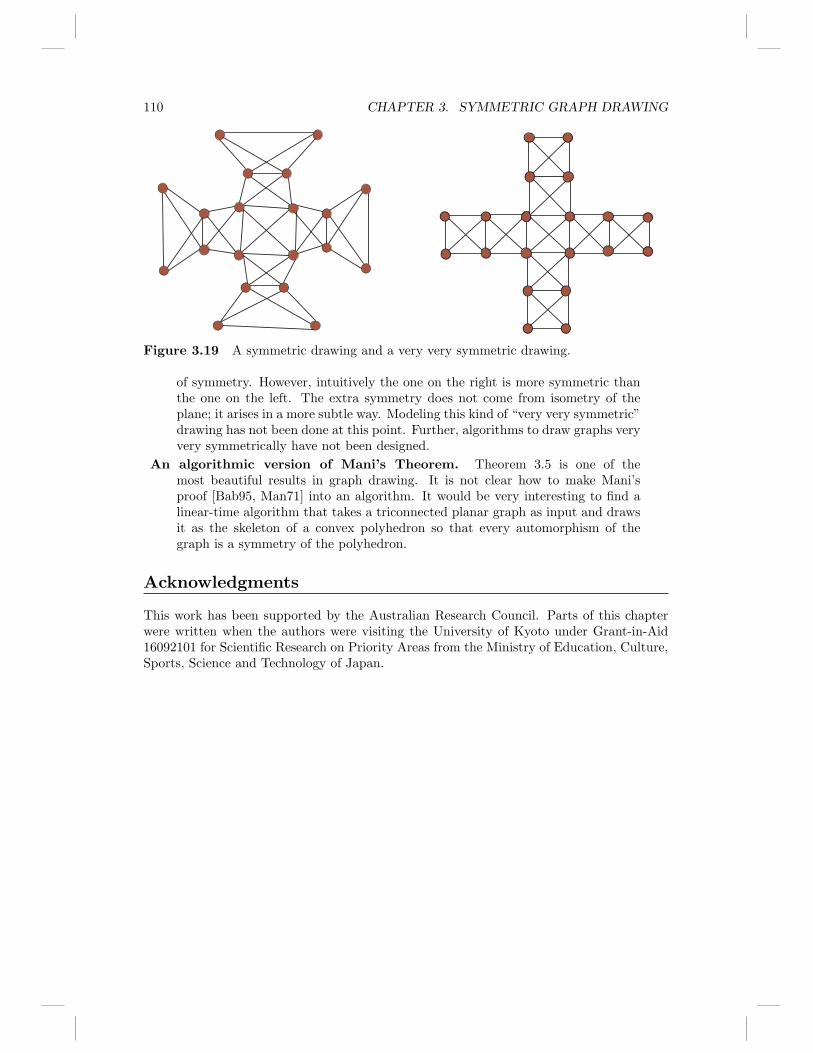
Very very symmetric graph drawing. Consider the two drawings in Figure 3.19.The two drawings, according to the model in Section 3.2.3, have the same degree


Figure 3.19 A symmetric drawing and a very very symmetric drawing.

of symmetry. However, intuitively the one on the right is more symmetric thanthe one on the left. The extra symmetry does not come from isometry of theplane; it arises in a more subtle way. Modeling this kind of “very very symmetric”drawing has not been done at this point. Further, algorithms to draw graphs veryvery symmetrically have not been designed.

An algorithmic version of Mani’s Theorem. Theorem 3.5 is one of themost beautiful results in graph drawing. It is not clear how to make Mani’sproof [Bab95, Man71] into an algorithm. It would be very interesting to find alinear-time algorithm that takes a triconnected planar graph as input and drawsit as the skeleton of a convex polyhedron so that every automorphism of thegraph is a symmetry of the polyhedron.

Acknowledgments

This work has been supported by the Australian Research Council. Parts of this chapterwere written when the authors were visiting the University of Kyoto under Grant-in-Aid16092101 for Scientific Research on Priority Areas from the Ministry of Education, Culture,Sports, Science and Technology of Japan.

REFERENCES 111

References

[AHT07] David Abelson, Seok-Hee Hong, and Donald E. Taylor. Geometric automor-phism groups of graphs. Discrete Applied Mathematics, 155(17):2211–2226,2007.

[AHU83] A. V. Aho, J. E. Hopcroft, and J. D. Ullman. Data Structures and Algo-rithms. Addison-Wesley, Reading, MA, 1983.

[AM88] M. J. Atallah and J. Manning. Fast detection and display of symmetry inembedded planar graphs, 1988.

[Arm88] M. A. Armstrong. Groups and Symmetry. Springer-Verlag, 1988.

[Bab95] L. Babai. Automorphism groups, isomorphism, and reconstruction. InGroetschel Graham and Lovasz, editors, Handbook of Combinatorics, vol-ume 2, chapter 27. Elsevier Science, 1995.

[Bac99] Sabine Bachl. Isomorphic subgraphs. In Kratochvıl [Kra99], pages 286–296.

[BJ01] Christoph Buchheim and Michael Junger. Detecting symmetries by branch& cut. In Mutzel et al. [MJL02], pages 178–188.

[BJ03] Christoph Buchheim and Michael Junger. An integer programming ap-proach to fuzzy symmetry detection. In Giuseppe Liotta, editor, GraphDrawing, volume 2912 of Lecture Notes in Computer Science, pages 166–177. Springer, 2003.

[CLY00] Ho-Lin Chen, Hsueh-I Lu, and Hsu-Chun Yen. On maximum symmetricsubgraphs. In Marks [Mar01], pages 372–383.

[CY02] Ming-Che Chuang and Hsu-Chun Yen. On nearly symmetric drawings ofgraphs. In IV, pages 489–, 2002.

[DETT99] G. Di Battista, P. Eades, R. Tamassia, and I. G. Tollis. Graph Drawing.Prentice Hall, Upper Saddle River, NJ, 1999.

[dF99] Hubert de Fraysseix. An heuristic for graph symmetry detection. In Kra-tochvıl [Kra99], pages 276–285.

[DT92] G. Di Battista and R. Tamassia. On-line planarity testing. Report CS-92-39, Comput. Sci. Dept., Brown Univ., Providence, RI, 1992.

[DTT92] G. Di Battista, R. Tamassia, and I. G. Tollis. Area requirement and symme-try display of planar upward drawings. Discrete Comput. Geom., 7(4):381–401, 1992.

[Ead84] P. Eades. A heuristic for graph drawing. Congr. Numer., 42:149–160, 1984.

[EL00] Peter Eades and Xuemin Lin. Spring algorithms and symmetry. Theor.Comput. Sci., 240(2):379–405, 2000.

[ELT96] P. Eades, X. Lin, and R. Tamassia. An algorithm for drawing a hierarchicalgraph. Internat. J. Comput. Geom. Appl., 6:145–156, 1996.

[FDK01] Karlis Freivalds, Ugur Dogrusoz, and Paulis Kikusts. Disconnected graphlayout and the polyomino packing approach. In Mutzel et al. [MJL02],pages 378–391.

[Fon76] M. Fontet. Linear algorithms for testing isomorphism of planar graphs. InProceedings Third Colloquium on Automata, Languages, and Programming,pages 411–423, 1976.

[HE00] Seok-Hee Hong and Peter Eades. An algorithm for finding three dimensionalsymmetry in trees. In Marks [Mar01], pages 360–371.


[HE03] Seok-Hee Hong and Peter Eades. Symmetric layout of disconnected graphs.In Toshihide Ibaraki, Naoki Katoh, and Hirotaka Ono, editors, ISAAC, vol-ume 2906 of Lecture Notes in Computer Science, pages 405–414. Springer,2003.

[HE05] Seok-Hee Hong and Peter Eades. Drawing planar graphs symmetrically, ii:Biconnected planar graphs. Algorithmica, 42(2):159–197, 2005.

[HE06] Seok-Hee Hong and Peter Eades. Drawing planar graphs symmetrically, iii:One-connected planar graphs. Algorithmica, 44(1):67–100, 2006.

[HEL00] Seok-Hee Hong, Peter Eades, and Sang Ho Lee. Drawing series paralleldigraphs symmetrically. Comput. Geom., 17(3-4):165–188, 2000.

[HEQL98] Seok-Hee Hong, Peter Eades, Aaron J. Quigley, and Sang Ho Lee. Drawingalgorithms for series-parallel digraphs in two and three dimensions. InGraph Drawing, pages 198–209, 1998.

[HME06] Seok-Hee Hong, Brendan D. McKay, and Peter Eades. A linear time algo-rithm for constructing maximally symmetric straight line drawings of tri-connected planar graphs. Discrete & Computational Geometry, 36(2):283–311, 2006.

[Hon01] Seok-Hee Hong. Drawing graphs symmetrically in three dimensions. InMutzel et al. [MJL02], pages 189–204.

[HT73] J. Hopcroft and R. E. Tarjan. Dividing a graph into triconnected compo-nents. SIAM J. Comput., 2(3):135–158, 1973.

[HW74] J. E. Hopcroft and J. K. Wong. Linear time algorithm for isomorphism ofplanar graphs. In Proc. of the Sixth Annual ACM Symposium on Theoryof Computing, pages 172–184, 1974.

[Kam88] T. Kamada. On Visualization of Abstract Objects and Relations. PhDthesis, Department of Information Science, University of Tokyo, 1988.

[Kam89] T. Kamada. Symmetric graph drawing by a spring algorithm and its ap-plications to radial drawing. Technical report, Department of InformationScience, University of Tokyo, 1989.

[KK89] T. Kamada and S. Kawai. An algorithm for drawing general undirectedgraphs. Inform. Process. Lett., 31:7–15, 1989.

[Kra99] Jan Kratochvıl, editor. Graph Drawing, 7th International Symposium,GD’99, Stirın Castle, Czech Republic, September 1999, Proceedings, vol-ume 1731 of Lecture Notes in Computer Science. Springer, 1999.

[Lin92] X. Lin. Analysis of Algorithms for Drawing Graphs. PhD thesis, Depart-ment of Computer Science, University of Queensland, 1992.

[LNS85] R. J. Lipton, S. C. North, and J. S. Sandberg. A method for drawinggraphs. In Proc. 1st Annu. ACM Sympos. Comput. Geom., pages 153–160,1985.

[Lub81] Anna Lubiw. Some np-complete problems similar to graph isomorphism.SIAM J. Comput., 10(1):11–21, 1981.

[MA86] J. Manning and M. J. Atallah. Fast detection and display of symmetry inouterplanar graphs. Technical Report CSD-TR-606, Department of Com-puter Science, Purdue University, 1986.

[MA88] J. Manning and M. J. Atallah. Fast detection and display of symmetry intrees. Congr. Numer., 64:159–169, 1988.

REFERENCES 113

[Man71] P. Mani. Automorphismen von polyedrischen graphen. Math. Annalen,192:279–303, 1971.

[Man90] J. Manning. Geometric Symmetry in Graphs. PhD thesis, Purdue Univ.,1990.

[Mar01] Joe Marks, editor. Graph Drawing, 8th International Symposium, GD 2000,Colonial Williamsburg, VA, USA, September 20-23, 2000, Proceedings, vol-ume 1984 of Lecture Notes in Computer Science. Springer, 2001.

[MJL02] Petra Mutzel, Michael Junger, and Sebastian Leipert, editors. Graph Draw-ing, 9th International Symposium, GD 2001 Vienna, Austria, September23-26, 2001, Revised Papers, volume 2265 of Lecture Notes in ComputerScience. Springer, 2002.

[RT81] E. Reingold and J. Tilford. Tidier drawing of trees. IEEE Trans. Softw.Eng., SE-7(2):223–228, 1981.

[SR34] E. Steinitz and H. Rademacher. Vorlesungen uber die Theorie der Polyeder.Julius Springer, Berlin, Germany, 1934.

[SR83] K. J. Supowit and E. M. Reingold. The complexity of drawing trees nicely.Acta Inform., 18:377–392, 1983.

[Tut63] W. T. Tutte. How to draw a graph. Proceedings London MathematicalSociety, 13(52):743–768, 1963.

[Tut66] W. T. Tutte. Connectivity in Graphs. University of Toronto Press, 1966.

[Wie64] Wielandt. Finite Permutation Groups. Academic Press, 1964.

[Won75] J. K. Wong. Isomorphism Problems Involving Planar Graphs. PhD thesis,Cornell Univ., 1975.

symmetric graph drawing - kit · symmetric graph drawing involves determining those automorphisms...

Documents