symcox 2015, stratigraphy and chemistry carbonate marker unit - copy

FACIES, STRATIGRAPHY, AND MINERALOGY OF THE CARBONATE MARKER AND

D MARKER UNITS, LOWER GREEN RIVER FORMATION, UINTA BASIN, UTAH

by

Carl Symcox

ii

A thesis submitted to the Faculty and the Board of Trustees of the Colorado School of

Mines in partial fulfillment of the requirements for the degree of Masters of Science (Geology).

Golden, Colorado

Date ______________________

Signed: _________________________

Carl Symcox

Signed: _________________________ Dr. J. Frederick Sarg

Thesis Advisor

Golden, Colorado

Date ______________________

Signed: _________________________ Dr. Paul Santi

Professor and Head Department of Geology and Geological Engineering

iii

ABSTRACT

This study documents and correlates the Carbonate Marker Unit and the D Marker Unit,

two regionally extensive carbonate beds within the Lower Green River Formation in the Uinta

basin. Both units were measured in a series of accessible canyons along the Roan Cliffs on the

southern margin of the basin. This was accomplished by incorporating measured outcrop,

petrographic analysis, X-ray fluorescence, X-ray diffraction, QEMSCAN analysis, and stable

isotopic analysis.

Four facies associations were identified that correlated to unique depositional

environments within the lake. These include delta, mudflat, shoal complex, and sublittoral

deposits. Facies associations were incorporated into a lacustrine depositional model to track

transgressive and regressive periods in the lake. Five transgressive-regressive cycles were

identified within the Carbonate Marker Unit and two in the D Marker Unit. Cycles were

observed in two distinct styles characterized by either rapid lake level fluctuation or by slow lake

level fluctuation. Some basal cycles in the Carbonate Marker Unit onlap onto the unit below as a

result of the dip component between the three canyons in this study. The D Marker Unit,

however, is a consistent thickness across all three sections as the result of a rapid transgression

which flooded all three sections simultaneously.

Lake Uinta during the lower Eocene Green River Formation is interpreted to be a closed-

lake system with water inputs controlled by monsoon-style seasonality and whose salinity varies

considerably. Two periods of freshwater are identified within the Carbonate Marker Unit,

characterized by the resurgence of mollusc taxa, broad swamps which hosted terrigenous plant

life sufficient to produce coals, and nutrient driven ostracod blooms. The upper freshwater period

in the Carbonate Marker Unit also corresponds with fish remains found in the formation.

Lake Uinta during Carbonate Marker and D Marker times is interpreted to be a stratified

lake with a well-developed chemocline. Beneath the chemocline waters were dense, highly

saline, reducing, and anoxic to dysoxic. As a result, precipitation of analcime cement, ferroan

dolomite, and the severe alteration or dissolution of clay species is common in the sublittoral and

profundal zones.

iv

TABLE OF CONTENTS

ABSTRACT ................................................................................................................................... iii

LIST OF FIGURES ....................................................................................................................... vi

LIST OF TABLES .........................................................................................................................xv

CHAPTER 1 INTRODUCTION ....................................................................................................1

CHAPTER 2 GEOLOGIC BACKGROUND .................................................................................4

2.1 Tectonic History and Stratigraphy ............................................................................4

2.2 Previous Interpretations ...........................................................................................8

2.3 Study Location .......................................................................................................11

CHAPTER 3 METHODS .............................................................................................................15

3.1 Outcrop Analysis ...................................................................................................15

3.2 Petrographic Analysis ............................................................................................15

3.3 X-Ray Fluorescence ...............................................................................................16

3.4 X-Ray Diffraction ..................................................................................................16

3.5 QEMSCAN Mineralogy and Porosity ...................................................................16

3.6 Stable Isotope Analysis ..........................................................................................17

CHAPTER 4 FACIES DESCRIPTION AND INTERPRETATION ...........................................18

4.1 Family 1: Sandstones .............................................................................................18

4.2 Family 2: Packstones, Grainstones, Floatstones, Rudstones .................................26

4.3 Family 3: Bioclastic Claystones and Siltstones .....................................................31

4.4 Family 4: Claystones and Siltstones ......................................................................32

4.5 Family 5: Carbonate Mudstones ............................................................................37

4.6 Coal ........................................................................................................................38

CHAPTER 5 FACIES ASSOCIATION AND STRATIGRAPHY .............................................43

5.1 Brief Summary of Lacustrine Deposition ..............................................................43

v

5.2 Facies Associations ................................................................................................44

5.3 Stratigraphic Correlation ........................................................................................54

CHAPTER 6 CHEMOFACIES AND MINERALOGY...............................................................66

6.1 X-Ray Fluorescence ...............................................................................................66

6.2 X-Ray Diffraction .................................................................................................75

6.3 QEMSCAN Mineralogy and Porosity ...................................................................83

6.4 Stable Isotope Analysis ..........................................................................................88

CHAPTER 7 DISCUSSION ........................................................................................................99

7.1 Paleo-Lake Uinta during the Lower Eocene ..........................................................99

7.1 Modern Analogs...................................................................................................102

CHAPTER 8 CONCLUSION....................................................................................................104

REFERENCES CITED ..................................................................................................................95

APPENDIX A: DETAILED MEASURED SECTIONS .............................................................114

APPENDIX B: XRF DATA ........................................................................................................142

APPENDIX C: XRD DATA .......................................................................................................146

APPENDIX D: QEMSCAN DATA ............................................................................................150

APPENDIX E: STABLE ISOTOPE DATA................................................................................161

vi

LIST OF FIGURES

Figure 1.1 Regional map of the Greater Green River and associated basins showing the bounding structures at the time of Green River Formation deposition. Modified after Tänavsuu-Milkeviciene & Sarg (2012). ..........................................3

Figure 2.1 Distribution of Laramide tectonic structures with respect to the Cretaceous/Paleogene basins. The Uinta basin is mostly a Laramide ponded basin bounded on all sides by tectonic uplifts. From Dickinson et al. (1988). ........5

Figure 2.2 Large scale depositional environment during the Late Paleocene. Small ponds and lakes west of the San Rafael Swell began to coalesce and fill the Uinta basin until it encountered the Douglas Creek Arch. Wasatch fluvial sands prograded from the south at this time. From Ryder, Fouch, and Elison (1976). .....6

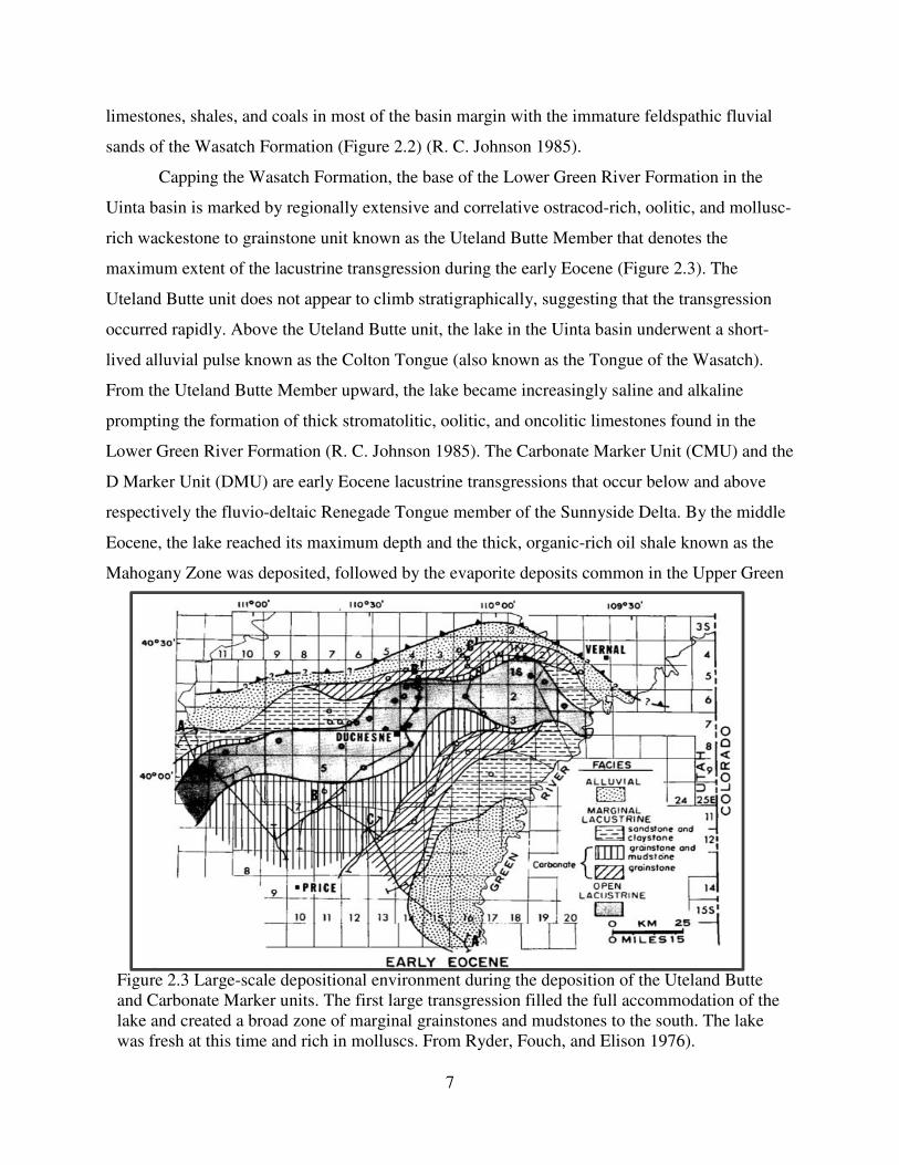
Figure 2.3 Large-scale depositional environment during the deposition of the Uteland Butte and Carbonate Marker units. The first large transgression filled the full accommodation of the lake and created a broad zone of marginal grainstones and mudstones to the south. The lake was fresh at this time and rich in molluscs. From Ryder, Fouch, and Elison 1976).....................................................7

Figure 2.4 Summary of the standardized stratigraphic nomenclature through the lower Green River and Wasatch Formations across the Greater Green River basin. The intervals highlighted in blue are the subject of this study. ...............................9

Figure 2.5 Large-scale stratigraphic interpretation of interaction of the southerly-derived siliciclastic system and the lacustrine cycles at the location of Nine Mile Canyon. Modified from Remy (1992) and Schomacker et al. (2010). ..................10

Figure 2.6 Example of a triple combo well log across the upper boundary of the CMU, where the argillaceous carbonate mudstones of the CMB lie beneath the detrital clay and sand-rich Sunny Side Delta (Renegade Tongue member). Well log and marked top provided by Anadarko Petroleum Company. ................12

Figure 2.7 Google Earth image showing the locations where sections were measured in this study and the outline of the Uinta basin. Distance between the Highway 191 Roadcut and Nine Mile Canyon outcrops is 26 km, and the distance between Nine Mile Canyon and Hay Canyon outcrops is 106 km. .......................13

Figure 4.1 Outcrop photos of Family 1: Sandstones. (A) Scour and fill sandstone with ostracods (lighter orange) entrained within the sedimentary structure. (B) Mud draped ripples. (C) Weathered carbonate and detrital grain lag, base of sharp-based sand. (D) Cross-stratified sandstone with weathered out mud rip-up clasts. (E) Burrows within climbing-rippled sand. (F) Grading up from distinct planar laminated ostracod bearing sandstone to an ostracod grainstone...22

Figure 4.2 Photomicrographs from Family 1: Sandstones. (A) F1.1, Calcite cemented sandstone containing large gastropod with sheltered porosity, ostracod shell

vii

fragments, and a large analcime grain. (B) F1.1, Laminations of compacted ostracods and sand. (C) F1.1, In XPL, a bivalve shell on the right has been half replaced with isotropic analcime and half with equant calcite. (D) F1.2, Equant poikilotopic cement filling bioturbation and entraining carbonate and detrital grains. (E) F1.2, Poorly sorted and compacted calcite cemented sandstone, non-grain supported cement likely was the result of dissolution/ reprecipitation of a calcareous matrix. (F) F1.2 Bioturbation within a calcareous laminated siltstone................................................................................23

Figure 4.3 Outcrop photos of Family 2: Carbonate Packstones-Rudstones. (A) Vertically stacked ostracod and oolite grainstones interbedded with siltstones and planar microbialites. (B) Interbedded ostracod grainstone and muddy microbialites. (C) Quartzose, carbonate floatstone rudstone (F2.3) between lime mudstones (F5.1). (D) Large rounded microbial balls (F2.5) in an oolite grainstone (F2.2). Note the bedding parallel surfaces. (E) Fining up sequence from an intraclast, pisolite rudstone to an oolite grainstone. Commonly found beneath well-developed domal or arborescent microbialites. .............................................27

Figure 4.4 Photomicrographs of Facies 2.1: Ostracod Packstones-Grainstones. (A) Unevenly distributed zones of densely packed ostracod shell fragments and matrix-rich packstone. (B) Well-cemented ostracod grainstone with preserved shell structures and filled with dolomitic mud. (C) Euhedral calcite and analcime cement growing into sheltered and intergranular dissolution porosity. (D) Calcite and analcime cement filling dissolution porosity. Note the patchy texture of intragranular muds against the preserved texture of intergranular mud. (E) Ostracod packstone with minor intragranular porosity. (F) From the same sample as E, ostracod grainstone with brecciated microbialite intraclasts, complete replacement with chert and microcrystalline silica. ......................................................................................................................28

Figure 4.5 Photomicrographs from Family 2: Carbonate Packstones-Rudstones. (A) F2.2, Micritization of an oolitic grain. (B) F2.2, Elongate oncolites with intragranular rims of dissolution porosity filled with calcite and analcime cement. (C) F2.2, Ostracod shell fragments, oncolites, and detrital quartz. Most porosity is filled with calcite cement. (D) F2.2, Oncolites and mixed carbonate intraclasts in a calcite cement, note the rind on the right most oncolite. (E) F2.2, Two intraclasts, one muddy bearing angular detrital grains and the other reworked calcite cement with oncolites entrained. (F) F2.4, Rock composed almost entirely of analcime with minor dolomite crystals and zones of birefringent illite. ...............................................................................................29

Figure 4.6 Outcrop photos of Family 3: Bioclastic Claystones and Siltstone. (A) F3.2 high spired gastropods and bivalves in a green-gray siltstone. (B) F3.2 mollusc shell fragments are commonly concentrated in thin beds. This suggests that deposition was close enough to wave base that currents or storms were periodically strong enough to create a shell lag. (C) F3.1 Argillaceous ostracod packstone to ostracod-rich claystone. Fissile in outcrop. ........................33

viii

Figure 4.7 Photomicrographs of Facies 3.1: Ostracod Claystone, Argillaceous Ostracod Wackestone. (A) Ostracods in a matrix of mud and silt. (B) Poorly sorted ostracod fragments with bone fragments. (C) Carbonate cement mixed with matrix in some samples. (D) High resolution of bone fragment. (E) Bone fragment adjacent to whole ostracod tests filled with dololime mud. ...................34

Figure 4.8 Outcrop Photos of Family 4: Claystones and Siltstones. (A) F4.1, Green siltstone with thin rippled sands. (B) F4.1, Thick section of gray silt (Jacob’s staff for scale). (C) F4.2, Light brown claystone in association with irregular lean dolomite intervals. Alternating clay and carbonates has been associated with non-seasonal sediment-flood to evaporative “whitings” cycles (Renaut and Gierlowski-Kordesch 2010). (D) F4.2, Black claystone associated with lean dolomitic mudstones. Differential compaction created an elongate lens of carbonate within a non-calcareous claystone. Similar to C, this may be the result of a hydrologic cyclicity. .............................................................................36

Figure 4.9 Outcrop Photos of Family 5: Carbonate Mudstones. (A) Carbonate Marker Bed at Highway 191 roadcut. Very thick bed of dolomitic lime mud (F5.2) and organic-rich dolomitic peloid packstone (F5.3). (B) Weakly brecciated laminated organic dolomitic peloid packstone associated with calm, deep water. (C) Carbonate Marker Bed at Nine Mile Canyon. Very thick bed of fissile argillaceous and quartzose dolomitic lime mud. (D) Laminated lean dolomitic lime mudstone, variable organic content. (E) Evidence of soft- sediment deformation slumping of a planar microbialite in the sublittoral. (F) Insect trace fossil found within an argillaceous dolomitic lime mudstone deposited along the shallow lake margin. ..............................................................40

Figure 4.10 Photomicrographs of Family 5: Carbonate Mudstones. (A) F5.1, Lime mudstone. Carbonate muds in the CMU and DMU rarely form without dolomite. Note black organic matter and white analcime cement. (B) F5.2, Mixed dolo-lime mud found in the CMB at Highway 191 roadcut, large zones of dissolved matrix filled with analcime cement. (C) F5.3, “Patchy” oxidation coloration of organic matter suggests variable permeability and oxidation potential during deposition and burial. (D) F5.3, Organic drapes (orange) over large dolomitic peloid aggregates. Several fish bones visible. (E) F5.3, Dolomitic peloid mudstone with visible silt and organic matter. (F) F5.4, Bioturbation crossing a silty laminae of a lean carbonate mudstone ......41

Figure 4.11 Outcrop Photos of Facies 6.1: Coals. (A) A 3cm laterally continuous coal seam in a thick bedded ostracod bearing carbonaceous siltstone (F3.1). (B) A 1.5cm discontinuous coal seam in a gray silt (F4.1). Calcareous, carbonaceous sandstone (F1.2) below and ostracod grainstone (F2.1) above. (C) Because common grasses had not become ecologically significant by the Eocene, terrigenous, lipid-rich plant matter that made up coals was primarily sourced from woody shrubs and trees. ................................................................................42

ix

Figure 5.1 Terminal distributary mouth bar prograding over a sharp-based mouth bar. This is indicative of a locally regressive lake level sequence. Measured in CMU at Nine Mile Canyon. ...................................................................................46

Figure 5.2 Two styles of deposition within the mudflat facies association. (A) Massive lime mudstone (F5.1) with two poorly sorted quartzose, carbonate floatstone, rudstone storm event beds (F2.3). (B) An intraclast, oolite rudstone (F2.3) overlain by fissile argillaceous carbonate mud (F5.1) with mudcracks. Mudcracks are filled with the grains from the unit above. ....................................49

Figure 5.3 Carbonate grain shoals. (A) Grading up from a calcareous sandstone (F1.2) to an ostracod grainstone (F2.1), lithology contact is orange line. (B) Grading up from a gray siltstone (F4.1) to an ostracod bearing sandstone (1.1) to an oncolite grainstone (2.2). .......................................................................................51

Figure 5.4 Facies found in the sublittoral facies association. (A) Alternating mixed dolo-lime mud (F5.2) and black claystone (F4.2) in what is interpreted as a whiting-flood cycle. (B) Synerisis cracks within black claystone. (C) Transitions from a green-gray siltstone into a whiting-flood cycle that has increasingly thick packages upward. Because detrital sediment input is linked to hydrologic input, the thicker beds of clay suggest greater hydrologic flux into the lake and a deeper lake. ......................................................................53

Figure 5.5 Comprehensive depositional model of ramp margin carbonates, colored by depositional environments. Observe that deltaic sandstones and littoral carbonates were deposited at the same depositional energy and lake depth. From Tänavsuu-Milkeviciene & Sarg, 2012. ........................................................55

Figure 5.6 Depositional model with respect to lake depth at the time of the CMU and DMU. The delta facies association encompasses a wide range of depositional energies that overlaps with the mudflat, shoal complex, and the sublittoral. The control for Track 1 or Track 2 deposition is determined by proximity to siliciclastic input. .........................................................................56

Figure 5.7 An example of a shallowing-upward sequence from a deep mud-draped rippled prodelta, to a sharp-based mouth bar, to an ostracod grainstone shoal, to a lime mudstone carbonate mudflat. From the CMU at Nine Mile Canyon. The transition from shoal complex to mudflat is indicative of a local change in sediment supply, reflected by the depositional tracks depicted in Figure 5.6. ......57

Figure 5.8 Cross section interpretation of the Carbonate Marker Unit across the three canyons included in this study. The section is oriented primarily in a strike direction with a dip component with 191 Roadcut being the most lakeward. The datum is at the top of the Carbonate Marker Bed in 191 Roadcut and Nine Mile Canyon, and at the fluvial channel that caps the Hay Canyon section. Measured section includes facies, facies association interpretation, and lake transgression and regressions. ................................................................................59

x

Figure 5.9 Each facies associations as a percent of the whole outcrop from each measured section in this study within the Carbonate Marker Unit. .......................61

Figure 5.10 Cross section interpretation of the D Marker Unit across the three canyons included in this study. The section is oriented primarily in a strike direction with a dip component with 191 Roadcut being the most lakeward. The datum is at the top of the first major flooding surface. Measured section includes facies, facies association interpretation, and lake transgression and regressions..............................................................................................................63

Figure 5.11 Each facies associations as a percent of the whole outcrop from each measured section in this study within the D Marker Unit. ....................................65

Figure 6.1 Ternary diagram of the major mineralogic components calculated from XRF analysis on all samples in this study, organized by lithologic family. Note that carbonate mudstones consistently contain a higher silicate component than the grain-rich lake-margin carbonates. Additionally, no sample measured more than 60% dolomite in this data set. ..................................70

Figure 6.2 Ternary diagrams of the major mineralogic components calculated from XRF analysis for Facies Families Sandstones and Packstones-Rudstones. F2.1 contains the most calculated silicates because it is often observed retaining intergranular matrix. In conjunction with the lack of grain coatings and is interpreted as medium-low energy marginal carbonates. ......................................71

Figure 6.3 Ternary diagrams of the major mineralogic components calculated from XRF analysis for Facies Families 3 and 4. Note within F3.1 there is substantial range of ostracod-to-clay ratio, but the amount of dolomite remains mostly stead between 10-20%. This may indicate a relationship between ostracod productivity in the locations where large volumes of detrital clay enters the lake. ........................................................................................................................72

Figure 6.4 Ternary diagrams of the major mineralogy components calculated from XRF analysis for Facies Families 5: Carbonate Mudstones. Many of the facies in this Family were identified and defined by their XRF analysis, therefore the separation and clustering of F5.1 and 5.2 on the ternary is a relic of their definition. Note that F5.4 clusters relatively closely around the center of the ternary as a relatively even distribution of dolomite, calcite, and silicates. ..........73

Figure 6.5 Synthetic gamma-ray response was constructed for each hand sample from the weight percent uranium, thorium, and potassium values obtained from XRF analysis. The data was plotted on a box and whisker plot in order to isolate statistical outliers; the sample size for each facies is given along the top of the plot. In this data set siliciclastic sandstones and mudstones show a high gamma-ray response due to anomalously high thorium and uranium content. Even when containing significant argillaceous component, carbonate mudstones and packstones still exhibit consistently clean gamma-ray response.

xi

Detrital mudstones and siltstones exhibit the largest standard deviation of calculated gamma-ray response. This may be the result of the challenge of finding fresh surfaces to XRF or the collected small sample. ...............................74

Figure 6.6 XRD plot with analysis accompanied by XRF weight percent oxides. Most relevant rock forming elements for this XRD plot highlighted in yellow. This figure demonstrates one example of a loss of clay speciation between the freshwater fluvio-deltaic source into the lake and into the saline, alkaline sublittoral or profundal. .........................................................................................77

Figure 6.7 XRD plot with analysis accompanied by XRF weight percent oxides. Most relevant rock forming elements for this XRD plot highlighted in yellow. Calcite was observed in all samples.......................................................................78

Figure 6.8 Dolomite is found in most or all locations within the lake, however volumetrically it is most prevalent in the deeper lake where the increased salinity from a preserved chemocline assists precipitation (Cole and Picard 1978). Very minor dolomite signature is observed in the floodplain sample, but none was observed in the nearshore. If the floodplains were periodically subjected to lacustrine waters then evaporation pumping of brine could concentrate the salt to higher concentrations than in the lake margins (Remy 1985). The profundal is the only sample that has evidence of significant dolomite, though its peaks are shifted....................................................................79

Figure 6.9 Dolomite that takes on Fe its crystal lattice creates a slight peak shift increase between 38° and 52° and can be detected in XRD. Ferroan dolomite requires more reducing conditions than in dolomite to form in order to accommodate the Fe into the lattice. It is only observed in this data set in the sublittoral/profundal zone. .....................................................................................80

Figure 6.10 Analcime is a common secondary precipitate mineral found in the CMU and DMU. Analcime forms in high salinity, high alkalinity, and moderate dissolved silica. Analcime was only observed in XRD in the sublittoral /profundal zone, however, it has been observed in thin section in porous carbonate grainstones and many carbonate mudstones filling dissolution porosity. .................................................................................................................81

Figure 6.11 QEMSCAN photo panel matching BSE image, porosity scan, and mineralogy scans of an ostracod packstone (Facies 2.1), an oncolitic grainstone (Facies 2.2), and an argillaceous ostracod wackestone (Facies 3.1). Samples show micritization, dissolution, and replacement of dolomitic mud and oncolites with calcite mud and cement..................................................................................85

Figure 6.12 QEMSCAN photo panel of matching BSE, porosity, and mineralogy scans of a dolomitic lime mudstone (Facies 5.2), a dolomitic peloid/intraclast lime wackestone (Facies 5.3A), and a dolomitic peloid packstone (Facies 5.3B).

xii

Mudstones deposited within the sublittoral exhibit dissolution of carbonate and reprecipitation of analcime cement. ................................................................87

Figure 6.13 Carbonate speciation as a function of pH. Above a pH of 11 essentially all dissolved carbon is in the form of carbonate ion. From Zeebe and Wolf- Gladrow, 2001........................................................................................................91

Figure 6.14 Depicts the correlation between δ13C and δ18O and the mineral speciation of carbonate. There is a moderate-to-strong correlation between δ18O and the precipitation of dolomite and no correlation between δ13C and the precipitation of dolomite. .......................................................................................93

Figure 6.15 Shows the δ13C and δ18O of the Carbonate Marker Unit in both the Highway 191 roadcut and Nine Mile Canyon. The Highway 191 roadcut exhibits strong isotopic covariance while the Nine Mile Canyon outcrop exhibits weak covariance. ....................................................................................................94

Figure 6.16 Depicts covarying trends of δ13C and δ18O with respect to depositional environment and controls from samples measured in this study. ..........................97

Figure 6.17 Depicts covarying trends of δ13C and δ18O with respect to depositional environment and controls from samples measured in this study and taken from the Coyote Wash 1 well analyzed in Pitman, 1996. This study finds that Pitman Primary trend and Pitman Diagenetic trend may instead be a relic of depositional pH and differential carbon fractionation in high pH systems .......98

Figure A.1 Facies key. In siliciclastics are colored to indicates sedimentary structure. In carbonates, the color represents the dominant grain type. Additional grains can be added to fully describe the sample. Pattern fills are used to express presence of dolomite, clay, and sand in a carbonate unit. ....................................114

Figure A.2 Facies Association Key. The facies associations in this study are broken into four environments: FA1: Deltaic, FA2: Mudflat, FA3: Shoal Complex, and FA4: Sublittoral. These colored interpretations are marked to the side of the measured section. .......................................................................................115

Figure A.3 Measured section of the Carbonate Marker Unit at Highway 191 roadcut. ........116

Figure A.4 Measured section of the Carbonate Marker Unit at Highway 191 roadcut continued. .............................................................................................................117



xiii








Figure A.14 Measured section of the Carbonate Marker Unit at Nine Mile Canyon. .............127

Figure A.15 Measured section of the Carbonate Marker Unit at Nine Mile Canyon continued. .............................................................................................................128







Figure A.22 Measured section of the Carbonate Marker Unit at Hay Canyon........................135

Figure A.23 Measured section of the Carbonate Marker Unit at Hay Canyon continued. .............................................................................................................136

xiv



Figure A.26 Measured section of the D Marker Unit at Highway 191 Roadcut. ....................139

Figure A.27 Measured section of the D Marker Unit at Nine Mile Canyon. ..........................140

Figure A.28 Measured section of the D Marker Unit at Hay Canyon. ...................................141

Figure C.1 Raw XRD data from a gray siliciclastic mudstone amongst non-calcareous sandstones and no ostracod fragments. Interpreted as deltaic floodplain. The Y-axis represents relative counts per second. ......................................................147

Figure C.2 Raw XRD data from an ostracod-rich claystone to argillaceous ostracod packstone interpreted as being deposited in nearshore, open lacustrine littoral zone. The Y-axis represents relative counts per second. ..........................148

Figure C.3 Raw XRD data from an argillaceous carbonate mudstone interpreted as being deposited in deep, open lacustrine sublittoral or profundal zone of the lake. The Y-axis represents relative counts per second. ................................149

Figure D.1 QEMSCAN results for Facies 2.1. ......................................................................151


Figure D.3 QEMSCAN results for Facies 3.1 ......................................................................153.

Figure D.4 QEMSCAN results for Facies 5.1 ......................................................................154.





Figure D.9 QEMSCAN results for Facies 5.3. .......................................................................159

Figure D.10 QEMSCAN results for Facies 5.3. .......................................................................160

xv

LIST OF TABLES

Table 2.1 Outcrop names and latitude and longitude coordinates at the base of section. ......11

Table 4.1 Bedding thicknesses with facies described in the CMU and DMU by Family. ....19

Table 5.1 Summary of facies associations, depositional subenvironments, and incorporated facies. ................................................................................................45

Table 6.1 Summary of mineral analysis and confidence XRD analysis. Clay analysis is reported as High, Medium, Low, or None relative to percent total clay. Non- clay minerals are reported as yes or no with degree of certainty: H=high certainty, L=low certainty. .....................................................................................82

Table B.1 XRF measurements of weight percent oxides of major rock forming elements, total calculated weight percent of the rock, and calculated gamma- ray response and organized by facies...................................................................142

Table D.1 Summary of samples analyzed by QEMSCAN with respect to facies and measured section. .................................................................................................150

Table E.1 Summary stable isotope measurements including sample, measured section, facies, δ18O, δ13C, weight percent calcite, and weight percent dolomite, and percent of carbonate as dolomite. ........................................................................161

1

CHAPTER 1

INTRODUCTION

The Uinta basin formed in the structural confines of the Sevier fold-and-thrust belt and

the Laramide thick-skinned orogenic zone as a broken foreland basin in what is now northeastern

Utah and northwestern Colorado. The Uinta basin was often filled by a massive lake that varied

widely in depth, geographic extent, and water chemistry. Sediment from the erosion of Laramide

and Sevier bounding structures were ponded into the subsiding lake basin.

The Eocene Green River Formation was deposited in the expansive lake complex within

the Uinta, Piceance, and Green River basins of Utah, Colorado, and Wyoming (Figure 1.1). The

largest and most long-lived of these lakes was Lake Uinta, which expanded across most of

northern present-day Utah and persisted throughout much of the Paleogene. The lacustrine

deposits found in the Uinta and Piceance basins are renowned for their vast unconventional

petroleum reserves hosted in organic-rich oil shales, which contain an abundance of kerogen

formed by algae and bacteria preserved within anoxic to dysoxic conditions on the lake bottom

(Ruble, Lewan, and Philp 2001). One of the-richest oil shales in the world is found in the upper

portion of the Green River Formation in what is known as the Mahogany Zone where the total

oil in place is estimated at 1.32 trillion barrels in the Uinta basin alone (R. C. Johnson, Mercier,

and Brownfield 2011). Because of their organic-richness and domestic availability, the oil shales

of the Uinta and Piceance basins are considered of high economic and strategic importance.

Although unconventional oil shale production has been the focus of research since the

1970’s as a result of the OPEC oil embargo (Andrews 2006), the majority of production in the

basin still comes from conventional plays targeting fluvio-deltaic and marginal carbonates where

reservoir quality is the highest. These plays are believed to be charged from deeper in the basin

where organic-rich source rocks generate hydrocarbons that migrate up-dip into shallower

reservoirs. However, attenuated well-log responses and highly heterolithic depositional

environments within the Green River Formation have provided challenges to correlating

stratigraphy into the subsurface, so laterally extensive marker units have been identified which

correlate lithologically across large portions of the basin (Cashion 1995; Tänavsuu-Milkeviciene

and Sarg 2012).

2

Two of the most prominent marker units in the Lower Green River Formation are the

Carbonate Marker Unit (CMU) and the D Marker Unit (DMU) that occur below and above

respectively the Renegade Tongue Sandy Member and outcrop along the southern margin of the

Uinta basin in the Roan Cliffs. The main objectives of this study were: 1) provide detailed litho-

and chemofacies observations on strata found within the CMU and DMU with respect to

lithology, mineralogy, and diagenesis; 2) document the depositional settings of marginal

carbonates and siliciclastics; and 3) provide an oblique strike and dip oriented stratigraphic

correlation along the southern margin of the basin to better understand lake cyclicity during

deposition. A better understanding of the depositional environments, stacking patterns, and facies

variability both along strike and dip has wide-ranging economic and academic implications

because these marker beds can be used as lithostratigraphic markers for stratigraphic correlation,

as potential reservoirs in the deeper basin, and as a systems analog for other shallow ramp

lacustrine systems actively being investigated in other areas of the world.

3

Figure 1.1 Regional map of the Greater Green River and associated basins showing the bounding structures at the time of Green River Formation deposition. Modified after Tänavsuu-Milkeviciene & Sarg (2012).

4

CHAPTER 2

GEOLOGIC BACKGROUND

2.1 Tectonic History and Stratigraphy

By the Late Cretaceous, the Sevier fold-and-thrust belt had created a series of northeast-

trending highland provinces across Utah and southwest Wyoming as the frontal part of the

greater Cordilleran retroarc thrust belt (Peter G. DeCelles 1994). Between Campanian and

Eocene times the Cordilleran thrust belt continued to migrate eastward forming several basins as

part of the compressional partitioning of the ramp-style Western Interior marine foreland basin.

This partitioning was supplemented by thick-skinned Laramide uplifts of fault-bounded blocks,

domes, and swells left from ancient tectonic systems, resulting in several irregularly distributed

basement-cored uplifts that form active basin margins throughout Utah, Wyoming, and

Northwestern Colorado (P. G. DeCelles and Coogan 2006). These Laramide foreland basins are

divided into perimeter basins, axial basins, and ponded basins by their confining geology and

hydrologic inputs/outputs (Dickinson et al. 1988). The Laramide basins formed during the Late

Cretaceous were roughly 35º N latitude at warm-temperate to sub-tropical climates and were

occupied by large lakes for much of the Paleogene time. These lake basins acted as regional

sediment traps, ponding the erosional sediments of the nearby Laramide uplifts (Roehler 1993;

Clementz and Sewall 2011).

The Uinta basin in northeastern Utah and westernmost Colorado is one of the largest ponded

basins and lies at the northern edge of the Colorado Plateau where it is bounded on all sides by

Laramide structures: the Uinta Uplift to the north, the San Rafael Swell to the southwest, and the

Uncompaghre uplift to the southeast (Figure 2.1). To the east the Douglas Creek Arch separates

it from the Piceance basin, but this structure was submerged during lake highstands. When the

Uinta and Piceance basins were connected they formed a vast lake named Lake Uinta that

covered approximately 20,000 km2 (M. D. Picard 1963; Lawton 2008; S. J. Davis et al. 2009).

The Uinta basin spans ~210 km along its east-west axis and ~160 km between its shallow

southern margin and its deeply faulted northern margin adjacent to the Uinta Uplift. The

depositional filling of the basin was highly asymmetric with over 4 km of sediment deposited

against the Uinta Uplift on the northern margin (Keighley et al. 2003). Over the Cretaceous and

Paleogene the occupying lakes (variety of names in the literature: Lake Uinta, Lake Flagstaff,

5

Figure 2.1 Distribution of Laramide tectonic structures with respect to the Cretaceous/Paleogene basins. The Uinta basin is mostly a Laramide ponded basin bounded on all sides by tectonic uplifts. From Dickinson et al. (1988).

6

Lake Gosiute) alternated several times between a closed-lake that collected all incoming

sediment, and an open-lake that would permit a limited outflow of sediment from the basin

(Tänavsuu-Milkeviciene and Sarg 2012).

During the Paleocene, several small isolated lakes and ponds in a western Sevier

transition basin west of the San Rafael Swell coalesced to form ancient Lake Flagstaff in the

Flagstaff basin. Over the course of the Paleocene, Lake Flagstaff expanded eastward filling in the

Uinta Basin until it encountered the Douglas Creek Arch anticlinal structural high (R. C. Johnson

1985). At this point, the Uinta basin was filled with a slightly alkaline, mostly freshwater lake

that deposited a thick limestone named the Flagstone Limestone as the lake filled.

Simultaneously, fluvial and alluvial sediments from the erosion of nearby uplifts began to

prograde into the basin. In the north, the uplift of the Uinta Mountains exposed the overlying

Mesozoic and Paleozoic sandstones, limestones, and marine shales. Erosion of these sediments

likely provided the dissolved calcium, magnesium, and anion molecules that saturated the lake

waters (Osmond 1965; Carroll, Chetel, and Smith 2006). From the south-southeast, a thick

sediment wedge developed from a persistent fluvial fan system replacing the upper Paleocene

Figure 2.2 Large scale depositional environment during the Late Paleocene. Small ponds and lakes west of the San Rafael Swell began to coalesce and fill the Uinta basin until it encountered the Douglas Creek Arch. Wasatch fluvial sands prograded from the south at this time. From Ryder, Fouch, and Elison (1976).

7

limestones, shales, and coals in most of the basin margin with the immature feldspathic fluvial

sands of the Wasatch Formation (Figure 2.2) (R. C. Johnson 1985).

Capping the Wasatch Formation, the base of the Lower Green River Formation in the

Uinta basin is marked by regionally extensive and correlative ostracod-rich, oolitic, and mollusc-

rich wackestone to grainstone unit known as the Uteland Butte Member that denotes the

maximum extent of the lacustrine transgression during the early Eocene (Figure 2.3). The

Uteland Butte unit does not appear to climb stratigraphically, suggesting that the transgression

occurred rapidly. Above the Uteland Butte unit, the lake in the Uinta basin underwent a short-

lived alluvial pulse known as the Colton Tongue (also known as the Tongue of the Wasatch).

From the Uteland Butte Member upward, the lake became increasingly saline and alkaline

prompting the formation of thick stromatolitic, oolitic, and oncolitic limestones found in the

Lower Green River Formation (R. C. Johnson 1985). The Carbonate Marker Unit (CMU) and the

D Marker Unit (DMU) are early Eocene lacustrine transgressions that occur below and above

respectively the fluvio-deltaic Renegade Tongue member of the Sunnyside Delta. By the middle

Eocene, the lake reached its maximum depth and the thick, organic-rich oil shale known as the

Mahogany Zone was deposited, followed by the evaporite deposits common in the Upper Green

Figure 2.3 Large-scale depositional environment during the deposition of the Uteland Butte and Carbonate Marker units. The first large transgression filled the full accommodation of the lake and created a broad zone of marginal grainstones and mudstones to the south. The lake was fresh at this time and rich in molluscs. From Ryder, Fouch, and Elison 1976).

8

River Formation across the Uinta and Piceance basins (Ryder, Fouch, and Elison 1976; Moncure

and Surdam 1980; Carroll, Chetel, and Smith 2006; Tänavsuu-Milkeviciene and Sarg 2012). A

summary of the nomenclature and stratigraphic order of the lower Green River Formation is

depicted in Figure 2.4. An interpretation of the large-scale transgressive and regressive cycles

during the lower Green River Formation is depicted in Figure 2.5.

2.2 Previous Interpretations

The early Eocene Green River Formation is composed of lacustrine and fluvio-deltaic

sediments deposited over approximately 10 Myr, from 54 to 44 Ma (Smith et al. 2010). The

Lower Green River Formation can be divided into a central core, composed of organic-rich

open-lacustrine hemipelagic claystone, carbonate mudstone, and oil shale, and the surrounding

ramp margin composed of cyclically interbedded marginal lacustrine ostracod and oolite

grainstone, argillaceous carbonate mudstone, and deltaic calcareous sandstone (Ryder, Fouch,

and Elison 1976). Broadly, the Green River Formation is separated into five lithological

members and seventeen kerogenous-rich and lean zones (R. C. Johnson 1985; Tänavsuu-

Milkeviciene and Sarg 2012). Throughout the Paleogene, the Uinta basin went through phases of

low regional erosion and restricted siliciclastic inflow where deposition was mostly driven by

precipitation of carbonates and evaporites. During wetter periods, sediment was supplied into the

Uinta basin from the erosion of the surrounding highlands, however sediment sources changed

often as tectonic activity continued throughout the Paleogene (Steven J. Davis et al. 2009).

Correlations within the Green River Formation are based on lithological marker units,

mechanical log markers, and microfossil suites. Although the most distinct marker bed is the

Mahogany Zone oil-shale bed in the upper Green River, the lower Green River Formation relies

on regionally correlative carbonate intervals as marker beds. The most prominent of these is the

Carbonate Marker Unit (CMU), a thick carbonate unit that, in general, separates the main body

of the Lower Green River Formation from the Wasatch Formation. In outcrops along the Roan

Cliffs, the CMU is capped by an organic-rich, regionally pervasive carbonate mudstone on the

order of 20 to 40 meters thick. The Carbonate Marker Bed (CMB) is identified in well log suites

by its distinct log response indicating the stratigraphic boundary between an organic-rich

carbonate mudstone and the overlying calcareous claystone and sandstones of the Renegade

9

Figure 2.4 Summary of the standardized stratigraphic nomenclature through the lower Green River and Wasatch Formations across the Greater Green River basin. The intervals highlighted in blue are the subject of this study.

10

Figure 2.5 Large-scale stratigraphic interpretation of interaction of the southerly-derived siliciclastic system and the lacustrine cycles

at the location of Nine Mile Canyon. Modified from Remy (1992) and Schomacker et al. (2010).

11

Tongue in this study (Figure 2.6) (Ryder, Fouch, and Elison 1976; Remy 1992). The CMU is

thickest along the ancient fluvial axis near Nine Mile Canyon and has been observed to decrease

in thickness both laterally along the margin and into the subsurface. The CMU has been

interpreted in the literature in a variety of ways: 1) as a lake-margin carbonate flat accumulating

along the fluctuating southern shore of Lake Uinta; 2) as a subaqueous mudflat; 3) as a crevasse-

splay; 4) as a shallow-lacustrine sand sheet; 5) as a delta distributary channel; and 6) as a

proximal open-lacustrine (Remy 1992; Fouch et al. 1976).

The stratigraphic and petrographic nature of the CMU and DMU in the Lower Green

River Formation are not well known as they change along strike and dip into the basin. Although

the marker units have historically been used as lithologic markers in outcrop and in the

subsurface, the stratigraphic and depositional context of the fresh water lower Green River

Formation transgressions are still poorly understood.

2.3 Study Location

The field area of this study include a series of accessible canyons along the Roan Cliffs

on the southern margin of the Uinta basin where good outcrop exposures are present. Three

outcrops were measured in a limited southeast-to-northwest oblique strike transect with a minor

dip component. The first site, Hay Canyon, is located approximately 27 km west of the

Colorado-Utah border and 45 km north of Cisco, Utah, and is the most marginal and off-axis of

the three measured sections. The second site, Nine Mile Canyon, is approximately 32 kilometers

northeast of Price, Utah, and 27 kilometers north of East Carbon, Utah, and is closely aligned to

a major hydrologic input of the Paleogene Lake Uinta. The third site is at the Highway 191

Roadcut located approximately 45 kilometers southwest of Duchesne, Utah and 30 kilometers

north of Price, Utah, and is the most western and lakeward of the three measured sections. A

summary of the field locations in this study is shown in Table 2.1 and Figure 2.7.

Table 2.1 Outcrop names and latitude and longitude coordinates at the base of section.

Outcrop Name Latitude Longitude

Hay Canyon CMU N39° 23.206’ W109° 23.120’

Hay Canyon DMU N39° 23.803’ W109° 23.643’

Nine Mile Canyon CMU N39° 46.694’ W110° 28.595’

Nine Mile Canyon DMU N39° 48.569’ W110° 21.352’

Highway 191 roadcut CMU N39° 50.461’ W110° 46.611’

Highway 191 roadcut DMU N39° 51.395’ W110° 45.572’

12

Figure 2.6 Example of a triple combo well log across the upper boundary of the CMU, where the argillaceous carbonate mudstones of the CMB lie beneath the detrital clay and sand-rich Sunny Side Delta (Renegade Tongue member). Well log and marked top provided by Anadarko Petroleum Company.

13

Figure 2.7 Google Earth image showing the locations where sections were measured in this study and the outline of the Uinta basin. Distance between the Highway 191 Roadcut and Nine Mile Canyon outcrops is 26 km, and the distance between Nine Mile Canyon and Hay Canyon outcrops is 106 km.

14

Each of the field locations had been previously measured as part of a large scale, low-

resolution stratigraphic analysis of the entire lower Green River Formation in the Uinta basin led

by Dr. Piret Plink-Björklund and Dr. Rick Sarg at the Colorado School of Mines. The

stratigraphic boundaries of the CMU and DMU for this study were roughly defined by the

previous work but were further defined above and below the CMU and DMU as the boundary

between fluvial dominated and deltaic/lacustrine dominated rock facies.

15

CHAPTER 3:

METHODS

The goal of this study was to provide detailed observations and analysis of rock facies

found in the CMU and DMU in order to infer depositional conditions and provide a stratigraphic

context for understanding lake cyclicity during their deposition. This was accomplished through

six analytical techniques listed below.

3.1 Outcrop Analysis

Fieldwork was conducted between August 2014 and February 2015. Measured sections

of the CMU and the DMU were done in each of the three study locations noted in Section 2.3.

GPS waypoints were taken at the base of each measured section. Each section was described

using a 1.6 m Jacob’s staff, 8% HCl acid, and hand lens. Observations were made on a

centimeter to meter scale while noting lithology, organic-richness, presence of biogenic remains,

sedimentary structures, nature of contacts, and large-scale bed geometry. Observations and

samples were documented with high-resolution photography. Approximately 175 hand

specimens were collected from the outcrops for subsequent analysis and observations.

Additionally, photomosaics of each measured section were taken to highlight macro-scale

architecture and to provide context for each measured section.

3.2 Petrographic Analysis

Fifty-four thin sections were prepared by Wagner Petrographic from hand samples

collected. Samples were cut to 30µm thicknesses and impregnated with blue dye epoxy to

highlight porosity. Half of the surface of each thin section was stained for calcite with Alizarin

Red S and also stained for iron. Samples were observed in plain polarized light (PPL), cross

polarized light (XPL), and in reflected light. Photomicrographs were taken through the optical

piece of a LABOPHOT2-POL NIKON transmitted light microscope. Observations were noted

with respect to lithology, sorting, fabric, texture, cement, and porosity.

16

3.3 X-Ray Fluorescence

All collected hand samples were analyzed by X-Ray Fluorescence (XRF) by an XL3t 950

GOLDD+ Niton XRF analyzer from Thermo Scientific. Samples were analyzed using the

TestALLGEO scan setting on an unweathered surface for a full three minutes. Raw elemental

data reported in parts per million was converted to percent weight oxides for most data analysis.

3.4 X-Ray Diffraction

Three clay-rich, unweathered samples were ground to a fine powder in a tungsten carbide

ball mill. The powdered material was subsequently analyzed using a Scintag XDS-2000 Θ-Θ

diffractometer and Cu Kα X-radiation by X-Ray Diffraction (XRD). Instrumental conditions

were 40 KV accelerating potential, 40 mA filament current, and 0.5 mm and 0.3 mm receiving

slits.

Continuous diffraction scans of randomly oriented bulk materials were obtained at a scan

rate of 1.0 degree/minute over the range of 4o-60o 2Θ. Oriented preparations of the clay-size

fraction (< 4um grain size) of each sample were then prepared by the Milliporetm filter transfer

method as described in Moore and Reynolds (1997) using a 0.45 micron filter. These

preparations were analyzed from 4o-40o 2Θ using the same instrumental parameters and a scan

rate of 1.0 degree/minute. Because the presence of a smectite group mineral was a possible

interpretation, all samples were ethylene glycol solvated and reanalyzed from ~1.5o-30o 2Θ at the

same instrumental conditions and a scan rate of 1.2 degrees/minute.

Ethylene glycol solvation enables identification of the presence of smectite group

minerals by causing a shift of the (001) basal reflection to lower 2-theta (e.g., 5.2o, which

corresponds to a basal spacing of ~17 Angstroms) relative to the air-dried sample. Detailed

discussion of these methods is provided in Moore and Reynolds (1997). Non-clay minerals were

identified using the ICDD powder diffraction file data base. Mineral identification by XRD is

possible if minerals are present in abundances greater than approximately 2 %. The actual limit

of resolution varies with mineral type.

3.5 QEMSCAN Mineralogy and Porosity

Quantitative Evaluation of Minerals by SCANning electron microscopy (QEMSCAN) is

probabilistic software that is capable of running on a specialized Scanning Electron Microscope

17

(SEM) equipped with four Energy-Dispersive x-ray Spectroscopy (EDS) detectors for rapid

scanning. Fifteen thin section samples were prepared by coating in carbon and analyzed three 1.5

mm2 areas per sample in a “porosity” scan (where only Backscatter Scattered Electrons (BSE)

are collected). Ten of the same samples were also analyzed in the same areas as the porosity scan

in a “mineralogy” scan (where EDS measurements are rapidly collected to build an elemental

map). From each scan the QEMSCAN software was capable of building porosity and

mineralogic maps based on common mineral suites, inputs, and directed user discretion.

3.6 Stable Isotope Analysis

Forty-one samples of carbonate mud were analyzed for δ13C and δ18O. Analysis of

oxygen and carbon stable isotopes for carbonate samples was performed at the Colorado School

of Mines Stable Isotope Laboratory. Carbonate samples for stable carbon and oxygen isotope

analysis were weighed to the equivalent of 90-120 µg CaCO3. Sample powders were digested

with 100% orthophosphoric acid on line at 90°C in a GV Instruments MultiPrep preparation

device. The resulting CO2 was cryogenically purified and analyzed by standard duel-inlet

techniques on a GV Instruments IsoPrime stable isotope ratio mass spectrometer. Corrections of

Craig (1957) were applied for the contribution of 17O, and all data are reported as a per mille (‰)

difference from the Vienna PeeDee Belemnite (VPDB) international reference standard.

Repeated analysis of an in-house carbonate standard, calibrated to VPDB via NBS (NIST) and

IAEA standards, has yielded an external precision of 0.03‰ for carbon, and 0.06‰ for oxygen

for this study.

18

CHAPTER 4

FACIES DESCRIPTION AND INTERPRETATION

Rocks in the Carbonate Marker Unit and D Marker Unit are divided into five families

based on lithologic composition. These are: 1) sandstones; 2) grain-rich limestones including

packstones, grainstones, floatstones, and rudstones; 3) bioclastic claystones and siltstones; 4)

unfossiliferous claystones and siltstones; and 5) carbonate mudstones composed of either calcite

or dolomite. Samples were then subdivided into facies by lithologic, structural, texture, and

mineralogic properties using methods discussed in Chapter 3. A summary of the facies by their

lithology, structure, thickness, geometry and contacts and depositional interpretation is provided

in Table 4.1.

4.1 Family 1: Sandstones

Facies 1.1 Mollusc, Ostracod, Oolite Sandstone: F1.1 is a very poorly-sorted silt to fine-

grained, matrix-rich sandstone bearing lacustrine derived carbonate bioclasts. Detrital grains are

almost entirely quartz, with minor chert and micas in some samples. Mud rip-up clasts can be

found, but rarely, in some samples. Sedimentary structures vary from current ripples, climbing

ripples, gradational planar, distinct planar, and cross-stratified. Minor scour and fill is observed

in some locations (Figure 4.1). Beds of F1.1 are commonly observed as sharp-based, tabular

beds, or as the lower portion that is gradationally overlain by a carbonate grainstone.

Molluscs are observed both as high spired gastropods and bivalves, with bivalves being

more common (Figure 4.2). Ostracod shell fragments are common in many samples, but can also

be found as articulated tests filled with a dark gray dolomitic mud, and commonly in bedding

parallel laminae (Figure 4.2). Calcite cement is observed in samples that are matrix poor, but is

patchy in distribution. Substantial intergranular porosity was observed in just two of ten thin

sections prepared of this facies. Sheltered porosity and dissolution porosity are found in most

samples, but vary in their extent, and rarely account for more than 1% of visible porosity in thin

section. In some samples the grains have the appearance of being ‘cement supported,’ suggesting

dissolution of a carbonate matrix that was then replaced with calcite cement. Analcime is

observed in samples replacing carbonate grains, mostly molluscs, as cement filling sheltered

porosity, or rarely as a reworked detrital grains (Figure 4.2). Bioturbation is

19

Table 4.1 Bedding thicknesses with facies described in the CMU and DMU.

Bedding Thickness Classes

Thickness (cm) Descriptive Term

100+ Very thick bed

30-100 Thick Bed

10-30 Medium Bed

3-10 Thin Bed

1-3 Very thin bed

0-1 Laminated

Family # Facies Name Lithology Structure Bed

Thickness

Geometries and

Contacts Interpretation

Facies

Associations

Sa

nd

sto

nes

1.1 Mollusc, Ostracod, Oolite

Sandstone

Very fine to fine sand, carbonate

grains. Can

contain clay/silt

or carbonate

mud; calcite or

analcime cement

Ripples, climbing ripples, gradational

planar, distinct

planar, cross-

stratified

Medium- thick bed,

rarely very

thick bed

Gradational with other sands or

grainstones or sharp-

based

Delta mouth bars, prodelta,

intershoal, shoal

FA1: Deltaic FA3: Shoal

Complex

1.2 Calcareous Argillaceous

Sandstone

Silt-very fine sand. Rip-up

mudclasts;

carbonate matrix

or cement

Distinct planar laminated, rippled or

climbing rippled,

scour and fill

Thin to very thick bed

Tabular or lenticular, gradational to sharp-

based. Usually

gradational tops

where preserved.

Distributary channel, delta

mouth bar,

prodelta, shoals,

sediment gravity

flow

FA1: Deltaic FA3: Shoal

Complex

FA4: Sublittoral

1.3 Non-carbonate Sandstone

Detrital quartz, feldspar, mica,

and chert. Minor

or no clay

matrix.

Grades upward from planar to scour-fill

and climbing ripples.

Most other structures

present but rare.

Medium to very thick

bed

Usually sharp-based and lenticular, but

can be gradational

and/or tabular in

outcrop scale

Distributary channel, delta

mouth bar, splay

sands.

FA1: Deltaic

20

Table 4.1 continued


Thickness

Geometries and


Facies

Associations

1.4 Bioclast, Oolite,

Quartzose

Conglomerate

Medium to very

coarse to detrital

quartz and

carbonate grains.

None Very thin

bed

Discontinuous,

erosional tops.

Base of sharp

delta mouth bar

FA1: Deltaic

Pa

ckst

on

es,

Gra

inst

on

es,

Flo

ats

ton

es,

an

d R

ud

sto

nes

2.1 Ostracod

Packstone-

Grainstone

Ostracods; Can

contain clay or

carbonate matrix

Planar laminated,

rippled, or cross-

stratified

Very thin to

very thick

bed

Sharp to gradational

bases, sharp top.

Tabular

Low to medium

energy carbonate

shoal deposit

FA3: Shoal

Complex

2.2 Oncolite, Oolite,

Pisolite,

Intraclast Grainstone

Oncolites and

oolites.

Intraclasts less common

Planar laminated,

rippled, or cross-

stratified

Very thin to

very thick

bed


bases, sharp top.

Tabular

High energy shoal

deposit

FA3: Shoal

Complex

2.3 Quartzose,

Carbonate

Floatstone-

Rudstone

Detrital and

carbonate grains,

mostly intraclasts

None Very thin to

very thick

bed


bases, sharp top.

Tabular

Very high energy

storm deposit

FA2: Mudflat

2.4 Intraclast

Analcimolite

Intraclasts and

analcime. Illite in

rare instances

None Very thin

bed

Sharp contacts, event

bed. Laterally

continuous

Mudflat or

sediment gravity

flow

FA2: Mudflat

FA4: Sublittoral

2.5 Microbialite

Boundstone

Carbonate

microbialites and

entrained grains

None Very thin to

medium bed

Sharp top and

bottom. Tabular,

event bed

All environments

with low-medium

energy and low

deposition

FA2: Mudflat

FA3: Shoal

Complex

FA4: Sublittoral

Bio

cla

stic

Cla

yst

on

es a

nd

Sil

tsto

nes

3.1 Ostracod

Claystone, Argillaceous

Ostracod

Wackestone

Clay, ostracods,

and very fine detrital quartz

Laminated, rippled Thin to very

thick bed

Gradational based

contact. Tabular on outcrop scale

Mudflat or calm

intershoal

FA2: Mudflat

FA3: Shoal Complex

3.2 Molluscan

Siltstone

Gray/green silt,

mollusc.

None Thin to very

thick bed

Tabular on outcrop

scale, sharp or

gradational contacts

Calm intershoal FA3: Shoal

Complex

21

Table 4.1 continued


Thickness

Geometries and


Facies

Associations C

lay

sto

nes

an

d S

ilts

ton

es 4.1 Green, Gray

Siltstone

Silt, minor clay

and carbonate

mud

None to weakly

laminated or rippled.

Rare soft sediment

deformation, mud

draped ripples, or ripples with sandy,

ostracod lenses

Very thin to

very thick

bed

Gradational tops and

bottoms except where

incised

Distributary

channel, delta

mouth bar,

prodelta,

mudflats, calm intershoal,

hypopycnal flow

FA1: Deltaic

FA2: Mudflat

FA3: Shoal

Complex

4.2 Brown, Black

Claystone

Clay, minor silt None to weakly

laminated or rippled.

Very thin to

very thick

bed

Sharp or gradational

tops and bottoms

Prodelta, mudflat

hypopycnal flow,

or gravity settling

FA2: Mudflat

FA4: Sublittoral

Ca

rbo

na

te M

ud

sto

nes

5.1 Lime Mudstone Lime mud and

detrital clay, silt

Massive or weakly

laminated

Very thin to

thick bed

Sharp-based or

gradational

Mudflat FA2: Mudflat

FA3: Shoal

Complex

5.2 Mixed Dolomite-

Lime Mudstone

Mixed calcite

and dolomite

mud. Minor

detrital silt and

clay

Massive or weakly

laminated

Very thin to

thick bed

Sharp-based or

gradational

Mudflat, calm

intershoal,

transitional

FA2: Mudflat

FA3: Shoal

Complex

FA4: Sublittoral

5.3 Organic Peloidal

Dolomitic

Wackestone to

Packstone

Dolomitic peloid

aggregates and

organic matter

Minor detrital silt

and clay

Laminated Very thin to

thick bed

Sharp-based or

gradational

Aggregated

precipitate,

gravitational

settling

FA2: Mudflat

FA4: Sublittoral

5.4 Laminated

Argillaceous Carbonate

Mudstone

Carbonate mud,

detrital silt and clay

Distinct laminations,

minor ripples, bioturbation

Very thin to

very thick bed

Sharp-based or

gradational

Authigenic

precipitate, gravitational

settling

FA2: Mudflat

FA4: Sublittoral

6.1 Coal Terrigenous

organic matter

None Very thin Sharp contact, wavy,

discontinuous in

places

Mudflat swamp FA2: Mudflat

22

Figure 4.1 Outcrop photos of Family 1: Sandstones. (A) Scour and fill sandstone with ostracods (lighter orange) entrained within the sedimentary structure. (B) Mud draped ripples. (C) Weathered carbonate and detrital grain lag, base of sharp-based sand. (D) Cross-stratified sandstone with weathered out mud rip-up clasts. (E) Burrows within climbing-rippled sand. (F) Grading up from distinct planar laminated ostracod bearing sandstone to an ostracod grainstone.

23

Figure 4.2 Photomicrographs from Family 1: Sandstones. (A) F1.1, Calcite cemented sandstone containing large gastropod with sheltered porosity, ostracod shell fragments, and a large analcime grain. (B) F1.1, Laminations of compacted ostracods and sand. (C) F1.1, In XPL, a bivalve shell on the right has been half replaced with isotropic analcime and half with equant calcite. (D) F1.2, Equant poikilotopic cement filling bioturbation and entraining carbonate and detrital grains. (E) F1.2, Poorly sorted and compacted calcite cemented sandstone, non-grain supported cement likely was the result of dissolution/reprecipitation of a calcareous matrix. (F) F1.2 Bioturbation within a calcareous laminated siltstone.

24

commonly observed in thin section crossing between irregular contacts of finer grained mud-rich

siltstones and coarser sandstones. Bioturbation is commonly either filled with a mix of detrital

components or equant calcite cement. One thin section of this facies from Highway 191 roadcut

contained 2 to 4 mm bone fragments (non-mineral calcium phosphate).

Interpretation: F1.1 are sands deposited within the lake that have either entrained lake-

derived carbonate grains during deposition or had organisms living in them after deposition. The

sharp-based, tabular geometry of the beds is the result of traction flow unconfined by a channel,

however the absence of bidirectional ripples suggests they are most commonly deltaic in origin

(Renaut and Gierlowski-Kordesch 2010; Schomacker et al. 2010). Sands of this facies are

interpreted as either deltaic, deposited within a delta mouth bar, splays, or as thin event beds

within the prodelta as a result of high sediment input, or as part of a wave-dominated shoal

complex where organisms commonly inhabit. In Nine Mile Canyon this facies is observed

grading into ostracod/oncolitic grainstones, suggesting that there is an intimate relationship

between delta mouth bars, splays, and carbonate shoals. Most mollusc species cannot survive in

the severe physical and chemical conditions of a fully saline lake (Williamson and Picard 1974),

therefore it is believed that bivalves and gastropods may indicate either a fresher lake or

proximity to a freshwater deltaic source.

Facies 1.2 Calcareous Argillaceous Sandstone: F1.2 is defined as a sandstone containing

between 15 to 40% carbonate as measured by XRF (see section 6.1) and not having substantial

observable carbonate grains. It is generally poorly-sorted to medium-sorted, contains clay or

carbonate mud matrix, and composed of silt and very fine sand. All samples exhibit medium to

strong bioturbation, occurring predominantly along grain size boundaries separating matrix-rich

zones from grain-rich zones. Some samples were observed to contain dissolution/reprecipitation

of equant or poikilotopic calcite or analcime, locally filling space left by bioturbation. Larger

detrital grains ranging from fine- to medium-grained are also observed filling burrows. This

facies is generally laminated or weakly rippled, but climbing ripples and scour and fill are also

observed. Beds range from a few centimeters to several meters thick. Bed geometries include

heterolithic lenticular channel, sharp-based tabular, and rarely as thin irregular and erosional

based.

25

Interpretation: F1.2 are sands that were deposited in the lacustrine environment but lack

entrained carbonate grains. Most of the sands in this facies are heavily bioturbated and exhibit

laminae of mud-rich and sand-rich sediment. Additionally, the sands are poorly sorted indicating

sediment transport flow was inconsistent and flashy. These sands are interpreted as deposited by

episodic traction flow sands and are interpreted as prodelta deposits or delta splays.

Facies 1.3 Non-carbonate Sandstone: F1.3 is defined as any sandstone with less than

15% carbonate or that does not fizz in outcrop within the Carbonate Marker and D-Marker units.

This facies is generally a well-sorted, very fine- to fine-grained sandstone found both in channel

lenses and tabular geometry. Root traces and long burrow bioturbation are observed in some

beds that are generally less than a meter thick. Rip-up clasts are found in the bottom 10 cm of

channel form geometries. Thin silty laminations are found in many places throughout larger

channel forms. F1.3 is generally more arkosic and immature than other sandstone facies.

Structures most commonly observed are climbing ripples, scour and fill, and distinct planar

laminations, but have been observed to contain ripples, soft sediment deformation, humpback

cross-stratification, and low angle convex up cross strata.

Interpretation: Sands within this facies are interpreted as being deposited with limited

exposure to the lake system during deposition and burial. These sands are locally lenticular in

geometry and can contain root traces or burrows. F1.3 is interpreted as being deposited by delta

distributary channel. Channels during the Eocene may have been ephemeral, allowing roots to

grow in the channel during dry spells. Scour and fill and rip-up clasts support the idea of

ephemeral high flow velocity channel systems associated with this facies. Climbing ripples

found in this facies also indicates that sediment load in these facies was high.

Facies 1.4 Bioclast, Oolite, Quartzose Conglomerate: F1.4 is a very poorly-sorted,

detrital medium- to coarse-grain sandy conglomerate, containing mud clasts, shell fragments,

oolites, and microbial fragment conglomerate. Beds ranged from 1 to 4 cm in thickness, are

discontinuous, highly weathered, contain no observable sedimentary structures, and are only

found at the base of sharp-based sandstones. This facies commonly weathers orange in outcrop

(Figure 4.1).

26

Interpretation: This facies is only found at the base of sandstone bodies. It is believed to

be the result of strong traction flow through underlying lacustrine sediments that were ripped up

and entrained in the flow. This facies is interpreted to be the result of strong currents coming off

the deltaic system and scouring into the lake bottom while building sharp-based mouth bars.

4.2 Family 2: Carbonate Packstones, Grainstones, Floatstones, and Rudstones

Facies 2.1 Ostracod Packstone-Grainstone: F2.1 is an ostracod packstone to grainstone

that can contain clay, calcite, or dolomitic mud. F2.1 is in many places associated and

interbedded with F2.6 muddy microbialite boundstones and F4.1 green, gray siltstones (Figure

4.3). In thin section, ostracod shells are commonly articulated and are filled with a dark gray

dolomitic mud, calcite and/or analcime cement, or show sheltered porosity. However, in some

samples compaction before cementation leaves bedding parallel shell fragments in a muddy

matrix. F2.1 can range from 'well-washed' fine-grained components to 'poorly-washed' where the

muds have a patchy intergranular texture in thin section. In some places, there are 2 to 5 cm thick

laterally continuous zones that have completely recrystallized into chert and silica (Figure 4.4).

F2.1 is generally composed completely of carbonate, but can contain up to 40% siliciclastics.

Dolomite can account for between 0% and 50% of measured carbonate depending on the volume

and composition of the matrix. One thin section of this facies from Highway 191 roadcut

contained 2 to 4 mm bone fragments.

Interpretation: This facies is likely deposited where wave energy was present to

concentrate carbonate grains, but weak enough to allow preservation of much of the intergranular

matrix. This facies is associated with the low energy edges and the distal portions of carbonate

shoal complexes (Cole and Picard 1978).

Facies 2.2 Oncolite, Oolite, Pisolite, Intraclast Grainstone: F2.2 is composed of coated

carbonate grains and intraclasts (Figure 4.5). Very fine- to fine-grained detrital quartz is common

in this facies, often filling the space between larger intraclasts. Intraclasts are mostly made of

fine-grained mud, both carbonate and clay, and commonly have shell fragments or detrital grains

entrained within them. Some intraclasts are highly elongate, suggesting brecciation from planar

microbialite. Unlike F2.1, samples from this facies contain little or no matrix, which indicates a

higher energy of deposition. Samples from this facies commonly

27

Figure 4.3 Outcrop photos of Family 2: Carbonate Packstones-Rudstones. (A) Vertically stacked

ostracod and oolite grainstones interbedded with siltstones and planar microbialites. (B)

Interbedded ostracod grainstone and muddy microbialites. (C) Quartzose, carbonate floatstone

rudstone (F2.3) between lime mudstones (F5.1). (D) Large rounded microbial balls (F2.5) in an

oolite grainstone (F2.2). Note the bedding parallel surfaces. (E) Fining up sequence from an

intraclast, pisolite rudstone to an oolite grainstone. Commonly found beneath well-developed

domal or arborescent microbialites.

28

Figure 4.4 Photomicrographs of Facies 2.1: Ostracod Packstones-Grainstones. (A) Unevenly distributed zones of densely packed ostracod shell fragments and matrix-rich packstone. (B) Well-cemented ostracod grainstone with preserved shell structures and filled with dolomitic mud. (C) Euhedral calcite and analcime cement growing into sheltered and intergranular dissolution porosity. (D) Calcite and analcime cement filling dissolution porosity. Note the patchy texture of intragranular muds against the preserved texture of intergranular mud. (E) Ostracod packstone with minor intragranular porosity. (F) From the same sample as E, ostracod grainstone with brecciated microbialite intraclasts, complete replacement with chert and microcrystalline silica.

29

Figure 4.5 Photomicrographs from Family 2: Carbonate Packstones-Rudstones. (A) F2.2, Micritization of an oolitic grain. (B) F2.2, Elongate oncolites with intragranular rims of dissolution porosity filled with calcite and analcime cement. (C) F2.2, Ostracod shell fragments, oncolites, and detrital quartz. Most porosity is filled with calcite cement. (D) F2.2, Oncolites and mixed carbonate intraclasts in a calcite cement, note the rind on the right most oncolite. (E) F2.2, Two intraclasts, one muddy bearing angular detrital grains and the other reworked calcite cement with oncolites entrained. (F) F2.4, Rock composed almost entirely of analcime with minor dolomite crystals and zones of birefringent illite.

30

have both calcite and analcime cements. The most common porosity observed in thin section was

sheltered porosity within ostracod grains and dissolution porosity within oncolites.

Interpretation: This facies represents the higher energy component of F2.1 and is

deposited along the high energy crests and or windward side of shoals. Higher wave energy

results in the complete winnowing of depositional mud, leaving high initial intergranular

porosity. Additionally, strong currents and wave energy roll grains around and allow for the

precipitation of grain coatings on oncolites and pisolites. (Cole and Picard 1978). Intraclasts are

the result of brecciation of other previously lithified rock due to high wave or current energy.

Many of the grains in this facies show a darkened microbial ‘rind’ on the outside of the edge of

the grain (Figure 4.5), however the relationship between microbial and authigenic coating of

grains is not clear from this study.

Facies 2.3 Quartzose, Carbonate Rudstone: F2.3 is a very poorly-sorted rudstone with

variable amounts of quartz sand that ranging from very fine to very coarse. Also present are

mollusc shell fragments, microbialite fragments, oolites and pisolites, and muddy intraclasts.

Commonly this facies is laterally continuous on outcrop scale and interbedded with lime

mudstone.

Interpretation: F2.3 contains poorly sorted detrital and lacustrine carbonate grains in

association with calm water lime mudstones. These are interpreted as storm deposits that washed

up of lacustrine sediments from the ramp and shoal complexes and deposited them onto the calm

nearshore mudflats and protected ramp margin.

Facies 2.4 Intraclast Analcimolite: F2.4 is an analcime and intraclast bearing rock with

more than 50% observed analcime in thin section (Figure 4.5). It is locally associated with

carbonate mudstones and grey siltstones. In some places, analcime is observed as cement filling

intergranular and intragranular pores associated with oval or elongate intraclasts (cement

occupies ~50% of rock), while in others the analcime appears to be separate grains and/or have

replaced carbonate clasts. The latter case has been observed with unevenly distributed zones of

illite. Thickness ranges between one and ten centimeters.

Interpretation: Concentrated analcime deposition in lakes occurs in areas of relatively

high salinity or high pH and elevated alkalinity (Remy 1985). This facies is interpreted as being

31

found either beneath the halocline of a well-stratified lake or along mudflats. In the deep lake,

density separation of more saline waters by hyperpycnal flows allows for concentration of brine

waters. On the mudflats along the margins of the lake the salinity of water is concentrated by

evaporative pumping during extended dry periods (Cole and Picard 1978; Remy 1985). Intraclast

grain flows observed within sublittoral mudstones are observed containing high volumes of

intergranular porosity completely cemented with analcime. Alternatively, extended periods of

evaporation along mudflats creates a hypersaline microenvironment which precipitates laterally

continuous beds of analcime along the lake shoreline.

Facies 2.5 Microbialite Boundstone: F2.5 is composed of all the mounded, domal, or

laminated mat deposits produced by microbial growth and metabolism. Hemispheroidal

stromatolitic or arborescent thrombolites are rare, but are still observed within the Carbonate

Marker and D-Marker units. The majority of microbialites are a few centimeter thick with fine-

grained laminations mats entrained within carbonate mud and interbedded with ostracod or

oncolite grainstones (Figure 4.3). This facies does not include brecciated microbialites, where

high energy has displaced the microbialite out of its growth position and deposited it as a large

carbonate grain within another facies. The bases of hemispheroidal or domed microbialites are

commonly observed above a high energy rudstone. In some locations peloids are trapped within

the lows of hemispheroidal microbialites, interpreted as periods of low sedimentation allowing

for extended rolling and displacement of pisolites and microbial growth.

Interpretation: Microbialites are deposited in any part of the lake that has access to

sunlight, low rates of sediment deposition, and is free of grazers. Therefore, microbialites can be

found in all the depositional environments between the mudflats and the sublittoral, depending

on the salinity and habitability of other organisms (Swierenga 2014). Most of the microbialites

found in this study are found within beds of carbonate mud and interbedded with carbonate

grainstone shoal deposits.

4.3 Family 3: Bioclastic Claystones and Siltstones

Facies 3.1 Ostracod Claystone, Argillaceous Ostracod Wackestone: F3.1 is a medium- to

well-sorted claystone to siltstone with ostracod tests. This facies is laterally continuous in

outcrop, and exhibits sharp contacts with grainstones and dolomitic mudstones. Most ostracods

32

are preserved as shell fragments but can be found as articulated bivalve tests filled with a dark

gray dolomitic mud (Figure 4.6). In some places, dissolution of the intragranular mud occurs and

is commonly replaced filled analcime or calcite cement. In general, very little porosity is

observed in thin section. One thin section of this facies contain 2 to 5mm fish bone fragments

(Figure 4.7).

Interpretation: F3.1 is the result of a mixed depositional environment of both detrital

clays and hemipelagic ostracods. The ratio of ostracod tests to detrital clay is variable in outcrop

suggesting either that wave energy was periodically capable of winnowing out clay or that there

were episodic blooms of ostracods in the lake. This facies is interpreted as being deposited in

calmer waters in the intershoals or in the protected area behind the shoals or anywhere laterally

along the coast protected from wave energy. The absence of molluscs suggests that the lake was

too saline or that locally the depositional environment was too far from a freshwater habitat

capable of supporting molluscs.

Facies 3.2Molluscan Siltstone: F3.2 is a gray siltstone containing both gastropods and

bivalves (Figure 4.6). Shells are found throughout this facies but are commonly concentrated in

bedding parallel shell lags approximately 1 cm thick (Figure 4.6). In general this facies is

approximately 30% bioclasts to 70% siltstone.

Interpretation: This facies contains green-gray detrital silt with gastropods and bivalve

molluscs. Because molluscs live in fresher water and this facies is coarser grained than F3.1, it is

interpreted as being closer to a freshwater source supplying detrital components. However, it is

also possible that the lake was fresher during intervals when this facies was deposited. This

facies is interpreted as being found in the calm intershoals or in the protected area behind shoals.

It often contains bedding parallel layers of mollusc debris and is interpreted as being affected by

storm wave energy or year-to-decade scale lake level fluctuations (Renaut and Gierlowski-

Kordesch 2010).

4.4 Family 4: Claystones and Siltstones

Facies 4.1 Green, Gray Siltstone: F4.1 is a siliciclastic siltstone to claystone, commonly

containing carbonate cement (Figure 4.8). It occurs mostly as massive to thinly laminated

33

Figure 4.6 Outcrop photos of Family 3: Bioclastic Claystones and Siltstone. (A) F3.2 high spired gastropods and bivalves in a green-gray siltstone. (B) F3.2 mollusc shell fragments are commonly concentrated in thin beds. This suggests that deposition was close enough to wave base that currents or storms were periodically strong enough to create a shell lag. (C) F3.1 Argillaceous ostracod packstone to ostracod-rich claystone. Fissile in outcrop.

34

Figure 4.7 Photomicrographs of Facies 3.1: Ostracod Claystone, Argillaceous Ostracod Wackestone. (A) Ostracods in a matrix of mud and silt. (B) Poorly sorted ostracod fragments with bone fragments. (C) Carbonate cement mixed with matrix in some samples. (D) High resolution of bone fragment. (E) Bone fragment adjacent to whole ostracod tests filled with dololime mud.

35

but in most locations it is too weathered to discern sedimentary structures. It can also contain

soft-sediment deformation, mud draped ripples, or rippled sandy or ostracod lenses, though less

commonly. F4.1 can range in thickness from centimeters to meters. It comprises laterally

continuous beds, interbedded with sands in a lenticular geometry, part of a lenticular heterolithic

channel fill, or as centimeter to decimeter thick beds within carbonate grainstones. It can contain

mudcracks filled with grains from the adjacent stratigraphic unit, such as oolites, ostracods, or

quartz sand. F4.1 most commonly weathers fissile, but can also weather in decimeter sized

nodules.

Interpretation: This facies is deposited either in a low-energy environment or as density

driven plumes (hypopycnal flows) extending into the lake where freshwater deltaic waters meet

saline lacustrine waters. Carbonate tests are not found within this facies, therefore it is deposited

either lakeward of carbonate shoals or within the prodelta at the edge of terminal splays of a

sublacustrine delta where lacustrine organisms are less common, or by rapid sedimentation as the

result of hypopycnal flows (Renaut and Gierlowski-Kordesch 2010). Depositional style depends

upon, salinity, density of the lake, and rate of sedimentation into the lake. Facies 4.1 may be

interbedded with sands of a delta mouth bar as the mouth bars move laterally and as sediment

supply changes through time.

Facies 4.2 Brown, Black Claystone: F4.2 is siliciclastic claystone with minor silt and

little to no carbonate (Figure 4.8) and is found weakly laminated or rippled. It weathers massive

or fissile in outcrop. F4.2 ranges from very thin to very thick bedded and is generally laterally

continuous, but can be incised by lenticular channel-form bodies. In some locations, it is

interbedded with massive or nodular beige dolomitic mudstones which can be laterally

continuous or lenticular.

Interpretation: This facies is found mainly associated with carbonate mudstones with few

or no coarser carbonate grains, and was deposited below fair weather wave base. The brown or

black color indicates the preservation of some organic matter, suggesting reducing conditions.

Rarely, brown mudstones are found within mudflats where conditions are reducing and the

waters are calm. The interbedded carbonate mudstones and non-calcareous claystones are

interpreted as hydrologic and sedimentologic cyclicity (not necessarily annual seasonality).

Flooding can provide large quantities of fresh water and sediment into the lake, slowing

36

Figure 4.8 Outcrop Photos of Family 4: Claystones and Siltstones. (A) F4.1, Green siltstone with thin rippled sands. (B) F4.1, Thick section of gray silt (Jacob’s staff for scale). (C) F4.2, Light brown claystone in association with irregular lean dolomite intervals. Alternating clay and carbonates has been associated with non-seasonal sediment-flood to evaporative “whitings” cycles (Renaut and Gierlowski-Kordesch 2010). (D) F4.2, Black claystone associated with lean dolomitic mudstones. Differential compaction created an elongate lens of carbonate within a non-calcareous claystone. Similar to C, this may be the result of a hydrologic cyclicity.

37

carbonate deposition and rapidly depositing clays into the calm sublittoral environment.

Subsequently, a return to carbonate deposition occurs. Modern analogs for this process are found

in the Dead Sea where summer “whitings” or the mixing of flood water and lake brine rapidly

deposit aragonitic mud (Talbot and Allen 1996).

4.5 Family 5: Carbonate Mudstones

Facies 5.1 Lime Mudstone: F5.1 is a carbonate mudstone containing more than 50%

calculated carbonate, but less than 15% calculated dolomite from XRF (see section 6.1). It is a

massive or weakly laminated depending on the clay content (Figure 4.9). This facies is generally

brown or white in outcrop but can also be found as a dark purple (Figure 4.10). F5.1 commonly

contains mudcracks filled with grains from overlying units.

Interpretation: Although calcite and dolomite muds are found throughout all depositional

environments of the lake, volumetrically the most calcite is deposited along the fresh water

margins of the lake (Cole and Picard 1978). F5.1 contains mudcracks due to periodic subaerial

exposure from lake level fluctuations. This facies is observed both as carbonate muds and as

argillaceous muds and is interpreted as low-energy carbonate portions of the ramp where the

energy has been dissipated (Platt and Wright 1991).

Facies 5.2 Mixed Dolomite-Lime Mudstone: F5.2 is a carbonate mudstone containing

more than 50% calculated carbonate, and more than 15% dolomite from XRF (see section 6.1)

and is commonly brown or black (Figure 4.9). This facies can contain up to 50% silicate

minerals and is a massive or weakly laminated depending on the clay and silt content. In thin

section, there is substantial dissolution of primary matrix, often replaced with analcime (Figure

4.10). This facies rarely contains ostracod tests, however the matrix is composed of calcareous

dolomicrite which differentiates it from Family 3.

Interpretation: F5.2 is interpreted as an authigenic carbonate deposit in calm water within

the lake. Because dolomite precipitates preferentially in more saline conditions, it is interpreted

as being deposited in any calm environment away from the freshwater margin (Pitman 1996).

Facies 5.3 Organic Peloidal Dololime Wackestone to packstone: F5.3 is a laminated to

weakly brecciated carbonate wackestone to packstone composed of dolomitic peloid crystal

38

aggregates and carbonate mud (Figure 4.10). This facies was only differentiated from F5.1 and

F5.2 by petrographic observations of amalgamated dolomitic peloid crystals, commonly draped

with organic matter. Bioturbation is observed rarely. Fish bone fragments (Figure 4.10), ostracod

shell fragments, and bivalve shell fragments are all observed rarely in thin section. Many

samples have a patchy light-dark coloration in thin section. Carbonate content ranges from 60%-

90% of whole rock sample, and calcite accounts from between 35%-55% of total carbonate.

Interpretation: F5.3 is laminated, organic-rich, and contains aggregates of dolomitic

peloids. This facies is interpreted as hemipelagic carbonate deposition during times of high

organic productivity by microbial processes. Microbial mediation of dolomite precipitation has

been observed in other systems (Breheret et al. 2008; Renaut and Gierlowski-Kordesch 2010;

Castanier, Metayer-Levrel, and Perthuisot 1999). These sediments are mostly laminated, but

show small evidence of brecciation in some places, suggesting it can be deposited farther

lakeward where it can be disturbed by ramp slope failure.

Facies 5.4 Laminated Argillaceous Carbonate Mudstone: F5.4 is a brown to black

carbonate mudstone with distinct laminations of silt and very fine detrital quartz (Figure 4.9 and

Figure 4.10). Trace bioturbation can be observed cutting across silty laminations. Laminations

can range in color from light gray, dark gray, dark brown, to light brown. Carbonate content

ranges from 60%-80% of whole rock sample, and calcite accounts from between 40%-75% of

total carbonate.

Interpretation: Lean, silty oil shale is interpreted as the hemipelagic settling of sapropel

below fair weather wave base in the sublittoral zone. Periodic silty laminations reach this zone,

but it remains mostly undisturbed. Although organic matter is preserved in this zone, both

bioturbation and the lean nature of the oil shale suggest it is not completely anoxic.

4.6 Family 6: Coal

Facies 6.1 Coal: F6.1 consists of thin beds of carbonized terrigenous organic matter

found within the lower portions of the CMU in all three canyons. These coals can be laterally

continuous or discontinuous in outcrop and are up to 3cm thickness (Figure 4.11).

Interpretation: Coal forms only in reducing conditions where there is sufficient

terrigenous organic matter. Because true grasses did not become ecologically abundant until the

39

Miocene (Leopold 1969), wetland swamps that deposited lacustrine coals were composed of

woody shrub and tree matter (Figure 4.11). Although reducing conditions are found throughout

the lake, this facies is interpreted as forming along shallow mudflats or nearshore swamps that

are likely to accumulate sufficient terrigenous organic matter. This is interpreted as the most

landward facies in this study.

40

Figure 4.9 Outcrop Photos of Family 5: Carbonate Mudstones. (A) Carbonate Marker Bed at Highway 191 roadcut. Very thick bed of dolomitic lime mud (F5.2) and organic-rich dolomitic peloid packstone (F5.3). (B) Weakly brecciated laminated organic dolomitic peloid packstone associated with calm, deep water. (C) Carbonate Marker Bed at Nine Mile Canyon. Very thick bed of fissile argillaceous and quartzose dolomitic lime mud. (D) Laminated lean dolomitic lime mudstone, variable organic content. (E) Evidence of soft-sediment deformation slumping of a planar microbialite in the sublittoral. (F) Insect trace fossil found within an argillaceous dolomitic lime mudstone deposited along the shallow lake margin.

CMB

41

Figure 4.10 Photomicrographs of Family 5: Carbonate Mudstones. (A) F5.1, Lime mudstone. Carbonate muds in the CMU and DMU rarely form without dolomite. Note black organic matter and white analcime cement. (B) F5.2, Mixed dolo-lime mud found in the CMB at Highway 191 roadcut, large zones of dissolved matrix filled with analcime cement. (C) F5.3, “Patchy” oxidation coloration of organic matter suggests variable permeability and oxidation potential during deposition and burial. (D) F5.3, Organic drapes (orange) over large dolomitic peloid aggregates. Several fish bones visible. (E) F5.3, Dolomitic peloid mudstone with visible silt and organic matter. (F) F5.4, Bioturbation crossing a silty laminae of a lean carbonate mudstone.

42

Figure 4.11 Outcrop Photos of Facies 6.1: Coals. (A) A 3cm laterally continuous coal seam in a thick bedded ostracod bearing carbonaceous siltstone (F3.1). (B) A 1.5cm discontinuous coal seam in a gray silt (F4.1). Calcareous, carbonaceous sandstone (F1.2) below and ostracod grainstone (F2.1) above. (C) Because common grasses had not become ecologically significant by the Eocene, terrigenous, lipid-rich plant matter that made up coals was primarily sourced from woody shrubs and trees.

43

CHAPTER 5

FACIES ASSOCIATIONS AND STRATIGRAPHY

5.1 Brief Summary of Lacustrine Deposition

Over geologic history expansive lacustrine systems have covered large provinces of

tectonically active continental basins and provided sites for deposition of thick sequences of

organic-rich sediments. However, lacustrine systems remain poorly studied relative to their

marine counter parts because they represent a much smaller percentage of the total rock record.

Because lacustrine depositional and hydrological systems are smaller than marine systems, they

respond more dynamically to changing sedimentologic and climatic variations. Studies of

lacustrine systems have demonstrated that they can have highly variable facies profiles both

laterally and temporally. As a result, understanding regional stratigraphy in highly cyclic

lacustrine systems has consistently proven challenging (e.g., M. Dane Picard and High 1972).

Analysis of lacustrine systems provides a unique set of challenges. Because they

represent a relatively small portion of the rock record and are inherently ephemeral in nature,

fewer analogs are available. Lacustrine systems differ from their marine counterparts in several

notable ways including:

• Lakes contain much smaller volumes of accommodation space to fill with sediment and

water. As a result, they are more sensitive to climate and tectonic controls on

accommodation and lake level.

• Lake shorelines can move large distances either by progradation or lake level fluctuation.

Changes of lake levels up to 300 meters in 15,000 years are not uncommon (Bohacs et al.

2000). Recently reservoirs in California have lost up to 90% of their reserves between

2012 and 2015.

• Lacustrine systems are dominated by waves and currents while tides are essentially

absent, even in large lakes.

• Because lakes are volumetrically limited, sediment supply and hydrologic inputs are

directly linked. Increased sediment supply is most often the result of increased influx of

water into the lake (e.g., Perlmutter and Matthews 1990).

• The existence of the lake is fundamentally tied to the rates of subsidence and filling of

accommodation, which is mainly the result of climate and tectonics (Bohacs et al. 2000).

44

Depositional environments within lakes are defined by energy levels. The shallow-water

zone above fair weather wave base is called the littoral zone. The littoral zone is characterized by

well-mixed, oxygenated waters due to wave energy. It may also experience significant

evaporation. The transitional zone between fair weather wave base and the storm weather wave

base is called the sublittoral zone. Beneath the storm weather wave base is the profundal zone,

which is often dysoxic or anoxic allowing for preservation of organic matter (Renaut and

Gierlowski-Kordesch 2010).

5.2 Facies Associations

The CMU and DMU were deposited during the early Eocene along the margins of a

fluvial-lacustrine lake controlled by accommodation and fill, which includes sediment and water

input (Bohacs 2001; Bohacs, Carroll, and Neal 2003). Sedimentologic controls and depositional

environments in the lake are interpreted by the use of facies associations. Facies associations are

packages of genetically related facies that occur in a single environment. To define facies

associations, the facies described in the previous chapter were related on the basis of texture,

lithology, stratigraphic relationships, and observations of modern fluvial-lacustrine systems. The

facies associations identified within the Carbonate Marker and D-Marker units are: 1) Delta, 2)

Mudflats, 3) Shoal Complex, and 4) Sublittoral (Table 5.1).

Facies Association 1: Delta

A lacustrine delta complex is composed of three depositional subenvironments: terminal

distributary channel, mouth bar, and prodelta.

Terminal distributary channels are the ends of fluvio-deltaic channels as they enter the

lake. Sedimentary structures associated with terminal distributary channels are planar

laminations, cross stratification, ripples, scour and fill, and climbing ripples. (Olariu et al. 2012;

Schomacker et al. 2010). They are best distinguished from other deltaic facies by their lenticular

geometry that often contains heterolithic fill of sand and silt (Figure 5.1). Terminal distributary

channels are highly susceptible to changes in lake level and hydrologic inputs. Fine-grained

overbank deposits and levee splays are also included in this depositional environment. Because

distributary channels most often contain fresh water runoff, they are the least likely to contain

45

Table 5.1 Summary of facies associations, depositional subenvironments, and incorporated facies.

Facies Association Depositional Subenvironments Facies

Deltaic (FA1) Distributary channels, mouth bars, prodelta

Mollusc, ostracod, oolite sandstone (F1.1); Calcareous argillaceous sandstone (F1.2); Non-carbonate sandstone (F1.3); Bioclast, oolite, quartzose conglomerate (F1.4); Green, gray siltstone (F4.1); Brown, black claystone (F4.2)

Mudflat (FA2) Mudflat, swamp

Quartzose, carbonate floatstone, rudstone (2.3); Intraclast analcimolite (F2.4)*, Microbialite boundstone (2.5); Ostracod claystone, argillaceous ostracod wackestone (F3.1); Green, gray siltstone (F4.1); Brown, black claystone (F4.2); Lime mudstone (F5.1); Mixed dolomite-lime mudstone (F5.2); Organic peloidal dololime wackestone to packstone (F5.3) Silty laminated “Oil Shale” (F5.4)*; Coal (F6.1)

Shoal Complex (FA3)

Shoal, intershoal

Mollusc, ostracod, oolite sandstone (F1.1); Calcareous argillaceous sandstone (F1.2); Ostracod packstone to grainstone (F2.1); Oncolite, oolite, pisolite, intraclast grainstone (F2.2); Microbialite Boundstone (F2.5); Ostracod claystone, argillaceous ostracod wackestone (F3.1); Molluscan siltstone (F3.2); Green, gray siltstone (F4.1); Mixed dolomite-lime mudstone (F5.2)

Sublittoral (FA4) Authigenic precipitate, Gravitational settling, Sediment gravity flow

Calcareous argillaceous sandstone (F1.2)*; Intraclast analcimolite (F2.4)*; Microbialite boundstone (F2.6); Brown, black claystone (F4.2); Mixed dolomite-lime mudstone (F5.2); Organic peloidal dololime wackestone to packstone (F5.3); Laminated argillaceous carbonate mudstone (F5.4)

*rare facies in respective facies association

46

Figure 5.1 Terminal distributary mouth bar prograding over a sharp-based mouth bar. This is indicative of a locally regressive lake level sequence. Measured in CMU at Nine Mile Canyon.

47

lacustrine derived grains and carbonate cementation. Facies associated with terminal distributary

channels in this study are calcareous argillaceous sandstone (F1.2), non-calcareous sandstone

(F1.3), and green, gray siltstone (F4.1).

Mouth bars are elongate bodies of sand deposited at the mouth of distributary channels

where the abrupt loss of channel confinement causes decrease in energy and deposition of

sediment bedload. Sedimentary structures found in mouth bars include rip-up clast

conglomerates, planar bedding, cross stratification, and climbing ripples (based on Schomacker

et al. 2010). Mouth bars by definition are not confined by channels, so in outcrop they are often

observed as tabular, sharp-based bodies of sand (Figure 5.1). Although scouring is uncommon,

the basal rip-up conglomerates and carbonate grain lags found at the base of some mouth bars is

evidence that it does occur. Facies in this study associated with mouth bars are mollusc, ostracod,

oolite sandstone (F1.1), calcareous argillaceous sandstone (F1.2), non-calcareous sandstone

(F1.3), bioclast, oolite, quartzose conglomerate (F1.4), and green, gray siltstone (F4.1).

A prodelta is the fine-grained distal end of deltaic clinoforms. Deposits are composed of

fine sands, silts, with some coarser grained material as a result of sediment gravity flows, often

identified by soft-sediment deformation. Sedimentary structures found in prodelta deposits are

structureless, planar lamination, and ripple topped fine sands. Ripples are often mud draped

(Figure 4.1 B). In outcrop, prodelta deposits are tabular with non-erosional contacts with the

underlying sediment, but can have erosional tops when capped by mouth bar deposits. Facies in

this study associated with the prodelta are mollusc, ostracod, oolite sandstone (F1.1), calcareous

argillaceous sandstone (F1.2), green, gray siltstone (F4.1), and brown, black claystone (F4.2).

Facies Association 2: Mudflat

Mudflats are the calm nearshore deposits along the shallow ramp edge of the lake.

Depositional subenvironments in this facies association include shallow mudflats and swamps.

Mudflat deposits in the CMU and DMU are noted for their low energy deposition and

high carbonate content. Along a ramp margin, vast areas can be covered in shallow, poorly

mixed waters. Due to the low angle of the lake margin, most wave energy generated in the lake is

lost before it reaches the shoreline, allowing for undisturbed, muddy deposition. Sedimentary

structures associated with mudflats are structureless, planar bedding, and minor rippling. One of

the most diagnostic features is the presence of mudcracks, which indicate periodic subaerial

48

exposure (Figure 5.2 B). Ten centimeter thick poorly sorted rudstone deposits, generally

dominated by carbonate grains and large intraclasts (Figure 5.2 A, B), may be interbedded with

the low-energy carbonate mudstones. Although dolomite can be deposited along mudflats,

volumetrically most carbonate in this environment is calcite (Cole and Picard 1978).

Additionally, when lake level is low and hydrologic communication with the lake along the

margins is poor, an environment of hypersalinity can be created due to evaporation pumping of

muddy sediments (Remy 1985). Broad platforms of shallow hypersaline waters have been

observed to produce centimeter thick beds of precipitated analcime. In this study, this was

observed only once as a 3 centimeter thick bed within the DMU at Nine Mile Canyon. Facies in

this study associated with mudflat deposits are quartzose, carbonate floatstones, rudstones (F2.3),

intraclast analcimolite (F2.4), microbialite boundstone (F2.5), ostracod claystone, argillaceous

ostracod wackestone (F3.1), green, gray siltstone (F4.2), brown, black mudstone (F4.2), lime

mudstone (F5.1), mixed dolo-lime mudstone (F5.2), and organic dolomitic peloid wackestone to

packstone (F5.3).

Swamp depositional subenvironments commonly contain peat or lignite. Peat-forming

environments are believed to have occurred along the quiet, freshwater, vegetated margin of the

lake (Hanley et al. 1976; Franczyk et al. 1989). Access to freshwater and terrigenous plant matter

requires that this depositional environment be near or adjacent to a freshwater hydrologic input.

Swamp deposits in this study are uniquely identified from other mudflat deposits by the presence

of coal (F6.1).

Facies Association 3: Shoal Complex

The shoal complex represents the high energy environment in the littoral zone. Shoals are

wave built structures that form due to positive feedback of elevated topography and wave

deposition. The zones between shoals are protected from full wave energy. The depositional

subenvironments described in this facies association are the shoal and intershoal.

The shoal is characterized by the highest energy lacustrine facies in the lake. Sedimentary

structures observed within carbonate shoals include planar laminations, rippled tops, and cross-

bedding. Lower energy back-shoals or leeward sides of shoals can preserve matrix, and as the

shoal crest is approached the matrix becomes winnowed away (Williamson and Picard 1974).

Grains along the shoal crest get rolled around and chemically agitated allowing for precipitation

49

Figure 5.2 Two styles of deposition within the mudflat facies association. (A) Massive lime

mudstone (F5.1) with two poorly sorted quartzose, carbonate floatstone, rudstone storm event

beds (F2.3). (B) An intraclast, oolite rudstone (F2.3) overlain by fissile argillaceous carbonate

mud (F5.1) with mudcracks. Mudcracks are filled with the grains from the unit above.

50

of grain coatings. Both oolitic and oncolitic textures were observed in this study. Intraclasts and

detrital sands may occur in the highest energy facies as reworked lacustrine sediments. Most

shoals observed in this study grade upward from a carbonate grain-bearing sandstone into a

packstone or grainstone (Figure 5.3 A, B). Periods of low energy or subaerial exposure allow for

muddy or microbial deposition onto a shoal. This is commonly observed in Nine Mile Canyon.

Facies in this study associated with shoal deposits are mollusc, ostracod, oolite sandstone (F1.1),

calcareous argillaceous sandstone (F1.2), ostracod packstone to grainstone (2.1), oncolite, oolite,

pisolite, intraclast grainstone (F2.2), and microbialite boundstone (2.5).

The intershoal subenvironment is characterized by lower energy muds, silts, and

bioturbation. Carbonate organisms are commonly found living in this portion of the lake. For

most of the CMU and DMU these are only ostracods, however during fresher times the lake

contained abundant molluscs. Thin shell lags of sediments found in this environment indicate

storm events that affected the lake bottom at these depths, and are most commonly found at the

bottommost portion of the CMU in the Highway 191 roadcut outcrops (Figure 4.6 B). Facies in

this study associated with intershoal deposits are mollusc, ostracod, oolite sandstone (F1.1),

microbialite boundstone (F2.4), ostracod claystone, argillaceous ostracod wackestone (F3.1),

molluscan siltstone (F3.2), green, gray siltstone (F4.2), and mixed dolomite-lime mudstone

(F5.2).

Facies Association 4: Sublittoral

The sublittoral zone in a lacustrine system is the zone between the fair weather wave base

and the storm weather wave base. Sediments in the sublittoral zone are the result of authigenic

precipitation of carbonate, gravitational settling, and sediment gravity flow deposits.

Carbonate precipitation in the sublittoral zone is ubiquitous. PaleoLake Uinta is believed

to have commonly been a poorly-mixed lake with a well-developed chemocline (M.D. Picard

1985; Bohacs 2001). The mixolimnion is the zone above the chemocline, whereas the

monimolimnion is the dense stratum beneath the chemocline that does not mix with the waters

above. In the mixolimnion layer where waters were well-mixed by wind, the lake is slightly

alkaline, well-oxygenated, and generally highly productive. In the monimolimnion layer where

waters are stratified and poorly-mixed, the waters are anoxic or dysoxic, saline, high pH, and low

eH. This separation occurs due to the density difference in waters caused by salinity and poor

51

Figure 5.3 Carbonate grain shoals. (A) Grading up from a calcareous sandstone (F1.2) to an ostracod grainstone (F2.1), lithology contact is orange line. (B) Grading up from a gray siltstone (F4.1) to an ostracod bearing sandstone (F1.1) to an ostracod grainstone/packstone (F2.1).

52

mixing of saline and fresher waters. Observations have shown that dolomite deposition is

volumetrically most prevalent in deeper portions of the lake (Cole and Picard 1978; Pitman

1996), but mechanisms for this remain unclear. Some recent studies have suggested microbial

activity is a mediating factor in dolomite precipitation (Castanier, Metayer-Levrel, and Perthuisot

1999; Breheret et al. 2008; Renaut and Gierlowski-Kordesch 2010), while others suggest that

salinity and sulfate reducing bacteria may induce dolomite precipitation (e.g., Van Lith et al.

2002). This study has observed organic-rich dolomitic peloid aggregate packstones draped with

organic matter that are believed to be the result of authigenic or pelagic crystallization of

dolomite or protodolomite in the water column and deposited beneath the chemocline. Facies in

this study associated with authigenic or pelagic sedimentation include microbialite boundstone

(F2.5), mixed dolomite-lime mudstone (F5.2), organic dolomitic peloid wackestone to packstone

(F5.3), and laminated argillaceous carbonate mudstone (F5.4).

Gravitational settling and thin sediment gravity flows are also associated with the

sublittoral zone. Unlike oceans, lakes often undergo overturning or drastic changes in chemistry

as a result of a heavy rains or floods. Heavy floods also bring in substantial amounts of sediment

into the water column. It has been suggested that interbedded carbonate mudstones and non-

carbonate claystones (Figure 5.4) may be the result of lacustrine whiting-flood pulses reflected in

the sublittoral zone (Figure 5.4A) (Talbot and Allen 1996; Renaut and Gierlowski-Kordesch

2010). Synerisis cracks and differential compaction have been observed in association with the

whiting-flood cycle deposits (Figure 5.4 B). Thin, 2 to 10 cm calcareous sandstones and

intraclast grain flows are rare in the CMU, and occur in thick packages of sublittoral dolomitic-

lime mudstones and have been interpreted as thin sediment gravity flows. The intraclast grain

flows commonly contain up to 50% intergranular porosity filled with analcime cement. Facies in

this study associated with gravitational settling and sediment gravity flows include calcareous

sandstone (F1.2), intraclast analcimolite (F2.4), brown, black claystones (F4.2), mixed dolomite-

lime mudstone (F5.2), organic dolomitic peloid wackestone to packstone (F5.3), and laminated

argillaceous carbonate mudstone (F5.4).

53

Figure 5.4 Facies found in the sublittoral facies association. (A) Alternating mixed dolo-lime mud (F5.2) and black claystone (F4.2) in what is interpreted as a whiting-flood cycle. (B) Synerisis cracks within black claystone. (C) Transitions from a green-gray siltstone into a whiting-flood cycle that has increasingly thick packages upward. Because detrital sediment input is linked to hydrologic input, the thicker beds of clay suggest greater hydrologic flux into the lake and a deeper lake.

54

5.3 Stratigraphic Correlation

Depositional Model

Several comprehensive lacustrine ramp margin depositional models have been proposed

in the literature (Bohacs 2001; Bohacs, Carroll, and Neal 2003; Renaut and Gierlowski-Kordesch

2010; Tänavsuu-Milkeviciene and Sarg 2012). The basis of the model developed in this study

comes from Tänavsuu-Milkeviciene & Sarg (2012); the model is shown in Figure 5.5. In this

model, deltaic and shoal complex facies associations occupy the same lake water depth and

depositional energy, but are controlled by access to a detrital sediment source. However the

model shows only a very narrow mudflat province.

Facies associations within the CMU and DMU suggest that across the shallow margin

there were large, shallow, low-energy mud depositional environments that were episodically

disrupted by storm events. Extended dry periods would expose mudflats to subaerial conditions,

while extended periods of evaporation would produce hypersaline waters which would produce

analcime rich deposits. Vegetated shoreline near freshwater inputs produced and deposited

terrigenous plant matter sufficient to develop coals. Additionally, prodelta deposits likely

extended into the sublittoral in places. To reflect these changes, this study has developed a

stratigraphic depositional model with respect to depth and sediment source (Figure 5.6). Track 1

represents a purely siliciclastic dominated interval while track 2 is a purely lacustrine dominated

interval. At any given time in the lake these environments would be lateral to one another and

could interfinger stratigraphically.

Using these depositional models as guidelines, measured sections were interpreted with

respect to their facies associations. From this, lake level transgressions and regressions were

interpreted. An example of a regressive cycle is shown in Figure 5.7. Lake transgressions and

regressions can be correlated across the entire lake, even if the facies belts are not continuous,

and were the criteria for developing time equivalent surfaces between outcrops. Stratigraphic

timelines were plotted to connect cyclic events in the lake. The detailed measured sections for

each canyon are in Appendix A.

55

Figure 5.5 Comprehensive depositional model of ramp margin carbonates, colored by depositional environments. Observe that deltaic sandstones and littoral carbonates were deposited at the same depositional energy and lake depth. From Tänavsuu-Milkeviciene & Sarg, 2012.

56

Figure 5.6 Depositional model with respect to lake depth at the time of the CMU and DMU. The delta facies association encompasses a wide range of depositional energies that overlaps with the mudflat, shoal complex, and the sublittoral. The control for Track 1 or Track 2 deposition is determined by proximity to siliciclastic input.

57

Figure 5.7 An example of a shallowing-upward sequence from a deep mud-draped rippled

prodelta, to a sharp-based mouth bar, to an ostracod grainstone shoal, to a lime mudstone

carbonate mudflat. From the CMU at Nine Mile Canyon. The transition from shoal complex to

mudflat is indicative of a local change in sediment supply, reflected by the depositional tracks

depicted in Figure 5.6.

58

Carbonate Marker Unit Stratigraphic Correlation

The results of the stratigraphic correlation of the CMU marker unit across the three

canyons in this study are shown in Figure 5.8.

The cross-section is taken in an oblique strike direction, but with a dip component where

the Highway 191 roadcut is the most lakeward section. The ramp angle between Hay Canyon

and Nine Mile Canyon averages 0.02° over 106 km, and the ramp angle between Nine Mile

Canyon and 191 Roadcut averages 0.06° over 26 km.

In general, the Highway 191 roadcut is dominated by low siliciclastic input siltstones and

ostracod-rich claystones that make up the sublittoral and mudflat environments. Nine Mile

Canyon is primarily composed of interbedded deltaic sandstones and siltstones and shoal

grainstones. Hay Canyon was the most landward outcrop, so was not exposed to the

transgression until later in the CMU. The facies associations at Hay Canyon are high energy

oolitic and oncolitic shoal deposits, some deltaic sand and silt facies, and well-developed

microbialites. A summary of the facies associations by percent of measured section (Figure 5.9)

shows that Nine Mile Canyon is dominated by deltaic facies whereas the Highway 191 roadcut is

off of the fluvial axis and composed mostly of grainstone shoals and mudflat carbonate muds and

fine-grained siliciclastics. Hay Canyon contains both high energy littoral oolitic and domal

microbialites, but also a substantial deltaic component. Preliminary petrographic observations

have indicated that the sands found within Hay Canyon are more mature and contain much fewer

micas and feldspars. This could indicate a different sediment source than Nine Mile Canyon or

the Highway191 roadcut, but further data would be required to confirm this hypothesis.

Using the model developed in Figures 5.5 and 5.6, lake level transgressions and

regressions were plotted and correlated across the measured section. Five cycles were identified

within the CMU characterized by two transgressive-regressive styles: rapidly fluctuating lake,

and gradually fluctuating lake. The lower three cycles are found within a rapidly fluctuating lake

and are characterized by slow regressions followed by rapid floodings and are colored in light

blue. The top two cycles are found within a gradually fluctuating lake and are characterized by

gradual regressions and transgressions and are colored in light green. Because of the dip

component of the measured section, the basal cycle onlapped onto the Colton Tongue between

the Highway 191 roadcut and the Nine Mile Canyon outcrop, and the two upper cycles of the

59

Figure 5.8 Cross section interpretation of the Carbonate Marker Unit across the three canyons

included in this study. The section is oriented primarily in a strike direction with a dip

component with 191 Roadcut being the most lakeward. The datum is at the top of the Carbonate

Marker Bed in 191 Roadcut and Nine Mile Canyon, and at the fluvial channel that caps the Hay

Canyon section. Measured section includes facies, facies association interpretation, and lake

transgression and regressions.

61

rapidly fluctuating lake cycles onlapped onto the Colton Tongue between the Nine Mile Canyon

outcrop and the Hay Canyon outcrop.

Coals were found in the lower portions of each of the three sections and are capped by

medium to thick-bedded ostracod packstones and grainstones. Coal-to-shoal deposits are

characteristic of the rapidly fluctuating lake and are most common in the basal cycles of the

Highway 191 roadcut. Molluscs, which have been interpreted as a proxy for fresh, hospitable

waters, were only found in the Highway 191 roadcut and Nine Mile Canyon sections near the

base of the section and near the base of the CMB. These are interpreted as the freshest periods

within the lake during the CMU.

The CMB was found capping the CMU in both the Nine Mile Canyon and 191 Roadcut

sections. In Nine Mile Canyon the CMB is an argillaceous and silty dolomitic-lime mudstone

containing variable organic content and increasing lime content upward deposited in the

sublittoral zone. The volume of silt found in the CMB at Nine Mile Canyon ranges from 10 to

30%, suggesting it was still near the fluvial axis at this time. The top five meters of the CMB are

heavily laminated, bioturbated, and up to 50% silt. This is interpreted as the early onset of the

fluvial pulse that marks the Renegade Tongue. At the Highway 191 roadcut, the CMB is a mixed

dolomitic-lime mudstone and dolomitic peloid packstones draped in organic matter with little to

Figure 5.9 Each facies associations as a percent of the whole outcrop from each measured

section in this study within the Carbonate Marker Unit.

0%

10%

20%

30%

40%

50%

60%

70%

80%

90%

100%

1 2 3

Facies Associations in the Carbonate Marker Unit

Series1 Series2 Series3 Series4

62

no siliciclastic input deposited in the sublittoral zone. Matrix dissolution and precipitation of

analcime cement in this outcrop is indicative of saline conditions beneath the chemocline. The

top of the CMB at the Highway191 roadcut grades into calcareous siltstones, thin ostracod

bearing sandstones, and ostracod grainstones before being incised by the fluvial-alluvial

sediment of the Renegade Tongue Member.

D Marker Unit Stratigraphic Correlation

The results of the stratigraphic correlation of the DMU marker unit across the three

canyons in this study are shown in Figure 5.10.

The DMU is a two to four meter lacustrine transgression that separates the Renegade

Tongue Member and the Sunnyside Delta Member of the Green River Formation. The cross-

section is in an oblique strike direction with a dip component where the Highway 191 roadcut is

the most lakeward section. The ramp angle between Hay Canyon and Nine Mile Canyon

averages 0.02° over 106 km, and the ramp angle between Nine Mile Canyon and 191 Roadcut

averages 0.06° over 26 km.

A summary of the facies associations by percent of the rock is shown in Figure 5.11. The

DMU at 191 Roadcut is dominated by sublittoral, organic-rich laminated mudstones with minor

beds of dark brown claystone. Planar microbialites within a carbonate mud were observed with

soft-sediment deformation features commonly associated with slope failure within the sublittoral

zone. The DMU at Nine Mile Canyon is an overall shallowing-upward sequence from carbonate

grain shoals to microbialite bearing carbonate mudflats. The unit is capped by hemispheroidal

domed microbialites that are immediately overlain by the sandy unit of the Sunnyside Delta

Member. At Hay Canyon the DMU is primarily composed of oolite to pisolite coated grainstones

and hemispheroidal domed microbialite structures. Pisolites were observed pooled between the

domes of low hemispheroidal microbialites, and is indicative of low sediment supply by which

the coated grains were able to roll around under the wave energy for an extended period of time.

Hay Canyon was deposited entirely in the high energy littoral zone.

The DMU consists of two cycles within a rapidly fluctuating lake. The datum was placed

at the top of the first cycle. Unlike the CMU, the thickness of the DMU cycles across all three

63

Figure 5.10 Cross section interpretation of the D Marker Unit across the three canyons included

in this study. The section is oriented primarily in a strike direction with a dip component with

191 Roadcut being the most lakeward. The datum is at the top of the first major flooding surface.

Measured section includes facies, facies association interpretation, and lake transgression and

regressions.

65

canyons is relatively constant, suggesting a rapid transgression that covered all three canyons

simultaneously. Molluscs were only observed at the base of the Highway 191 roadcut, and well-

developed microbialites are much more common in the DMU. Both of these suggest conditions

in the lake had become less favorable for biodiversity.

Figure 5.11 Each facies associations as a percent of the whole outcrop from each measured

section in this study within the D Marker Unit.

0%

10%

20%

30%

40%

50%

60%

70%

80%

90%

100%

1 2 3

Facies Associations in the D Marker Unit

Series1 Series2 Series3 Series4

66

CHAPTER 6

CHEMOFACIES AND MINERALOGY

Lacustrine sediments in the Green River Formation exhibit complex mineral suites that

are not easily quantified in hand sample or petrographic analysis. Many samples contain fine-

grained dolomite, calcite, clay, analcime, quartz, and other minerals that cannot be easily

quantified through traditional observations. A suite of chemical analysis was performed on the

samples to elucidate on the mineralogic and isotopic trends found within the CMU and DMU.

6.1 X-Ray Fluorescence

Calculated Mineralogy

XRF allows for a more quantified description of the elemental makeup of samples, and

can be used with equations to quantify the mineral composition of samples. All hand samples

taken from the measured outcrops were analyzed with XRF in order to infer mineral composition

and to calculate an anticipated gamma-ray response for each facies.

XRF is the process by which high-energy X-rays are targeted at a material to dislodge

inner electrons from atoms. When this happens, an outer electron ‘falls’ into the place of the

dislodged electron and releases energy equivalent to the difference between the binding energies

of the inner and outer electrons. Because the orbital energy differential for each element is

unique, the wavelength of light emitted by an ionized atom gives information on the element

being observed. Although XRF can theoretically detect X-ray emissions from virtually all

elements, the commercially available sampler in this study cannot measure the abundances of

elements with an atomic number of less than 11. Therefore, mineralogy assumptions have to be

made from heavier elements in order to infer the composition of the sample. For example,

because carbon and oxygen are too light to be measured by the XRF, and calculations of the

amount of calcite in a sample relies solely on presence of calcium. XRF also cannot provide

information to the mineral structure or location of the elements in the measured sample.

To calculate bulk mineralogy in the samples, several assumptions were made about the

partitioning and oxidation states mineral forming elements measured with XRF. The following

assumptions were made in calculating calcite, dolomite, and total silicates followed by the

known mineralogy limitations of the assumptions:

67

1. All Mg is in dolomite

• There is high and low Mg calcite in the Green River Formation (Pitman 1996)

• Detrital illite, chlorite, and smectite group clays can incorporate Mg into their

mineral structure

2. All Ca not in dolomite is contained in calcite

• Plagioclase feldspar and smectite group clays can incorporate Ca into their

mineral structure

• Gypsum and anhydrite are common weathering surfaces on outcrop rocks and if

measured can greatly overestimate Ca content

From these assumptions, equations were derived that estimate the weight percent of silicates

(Equation 1), calcite (Equation 2), and dolomite (Equation 3).

(Equation 1)

(Equation 2)

(Equation 3)

(Concentration measured in parts per million, MW=Molecular Weight)

The calculated mineral percent composition was plotted onto ternary diagrams where each axis

represented the calculated weight percent of that mineral solely with respect to the three end

members. All other minerals and elements measured by XRF were not included in the total

weight percent. The axes of the ternary diagram are calculated silicates, calculated calcite, and

calculated dolomite. The calculated whole rock mineralogy of all samples collected in this study

is depicted in Figure 6.1, organized by lithologic family; the calculated whole rock mineralogy

within each facies is given in Figures 6.2, 6.3, and 6.4.

68

Gamma-ray response

Gamma-ray response was calculated from the XRF data using Equation 4, derived from

the decay constants of the three most common radioactive elements found in earth minerals:

Uranium, Thorium, and Potassium.

(Equation 4)

(Concentration in parts per million)

Gamma-ray response was then calculated and plotted by facies (Figure 6.5). The Green River

Formation commonly exhibits unusual gamma-ray patterns, so many facies had statistical

outliers. To account for this, the calculated gamma-ray response was depicted using a box and

whisker plot to show the expected spread in gamma-ray values while also showing statistical

outliers. In a box and whisker plot the innermost line represents the median, whereas the width of

the box represents the distance from the median to the 1st and 3rd quartile. The lines extending

from the ends of the box represent the same distance from the median to the end of the box, so

twice the distance from the median to the 1st and 3rd quartiles. All data that plots more than twice

the distance between the median and the 1st or 3rd quartile is considered a statistical outlier.

XRF Observations:

The following observations were made with regard to calculated mineralogy from XRF

on each of the facies families in the CMU and DMU:

The distribution of mineralogy of all samples in this study is shown in Figure 6.1. There

is an unoccupied space of rocks that contained low weight percent calcite. Samples in this study

never contained less than 30% carbonate unless they contained more than 65% siliciclastics.

Siliciclastic sandstones and mudstones rarely contained more than 10 weight percent dolomite.

Carbonate mudstones found along mudflats and in the sublittoral zone have a high calculated

siliciclastic input relative to carbonate grainstones. Two hypotheses are presented to explain this.

First, carbonate muds deposited along mudflats and in the sublittoral are exposed to calm waters

where preservation potential of the fine argillaceous component is high. This would suggest that

even in times of high carbonate deposition and low siliciclastic input there is still a pervasive

69

settling and deposition of clays throughout most of the lake, whereas depositional environments

where grainstones are deposited clays are winnowed away. The second hypothesis is that

analcime is commonly precipitated in the sediments deposited beneath the halocline or along the

mudflats where conditions are often hypersaline. Analcime is a sodium aluminosilicate pseudo-

zeolite with chemical formula similar to albite. Substantial authigenic analcime could increase

the XRF response for both silica and aluminum.

The distribution of mineralogy of grain-rich carbonates is shown in Figure 6.2. Ostracod

packstones to grainstones (F2.1) are deposited in calmer leeward shoals where clay-carbonate

matrix is commonly preserved. As a result, the samples in F2.1 commonly show elevated silicate

content and can contain up to 40% siliciclastics. Furthermore, oncolite, oolite, pisolite, intraclast

grainstones (F2.2) generally exhibit higher dolomite content than uncoated ostracod grains in

F2.1. The coatings on oncolitic and oolitic grains are commonly composed entirely of dolomite.

Additionally, intraclasts in this facies are generally dolomite rich. The high silicate outlier in

F2.1 was analyzed along a zone completely recrystallized in silica (see Figure 4.4 F).

The distribution of mineralogy of bioclastic claystones and siltstones is shown in Figure

6.3. Ostracod claystones to argillaceous ostracod wackestones (F3.1) exhibit a wide range of

calcite and silicate compositions. This compositional range is the result of the ostracod

productivity and sedimentologic variability in the lake. Ostracod blooms result from increased

nutrients increase the calcite content in the underlying sediment when they are deposited, while

increased hydrologic inflow increases the detrital clay component. Dolomite content within F3.1

is generally less than 20%.

The distribution of mineralogy of carbonate mudstones is shown in Figure 6.4. Carbonate

mudstones in this study are generally a compositional mixture of calcite and dolomite with

between 10 to 40 weight percent silicates. Carbonate mud composition abruptly stops before

becoming less than 30 weight percent calcite. The samples with the highest dolomite

composition are composed of dolomitic peloid aggregate crystals.

Some samples in this data set are observed plotting with negative calcite values. All

magnesium within this study is defined as residing in dolomite, and the equation pairs a calcium

atom for every measured magnesium atom. If the magnesium is derived from a non-carbonate

source and there are insufficient calcium atoms to pair with measured magnesium atoms, a

70

Figure 6.1 Ternary diagram of the major mineralogic components calculated from XRF analysis on all samples in this study,

organized by lithologic family. Note that carbonate mudstones consistently contain a higher silicate component than the grain-rich

lake-margin carbonates. Additionally, no sample measured more than 60% dolomite in this data set.

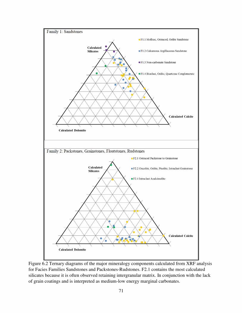
71

Figure 6.2 Ternary diagrams of the major mineralogy components calculated from XRF analysis

for Facies Families Sandstones and Packstones-Rudstones. F2.1 contains the most calculated

silicates because it is often observed retaining intergranular matrix. In conjunction with the lack

of grain coatings and is interpreted as medium-low energy marginal carbonates.

72

Figure 6.3 Ternary diagrams of the major mineralogic components calculated from XRF analysis

for Facies Families 3 and 4. Note within F3.1 there is substantial range of ostracod-to-clay ratio,

but the amount of dolomite remains mostly stead between 10-20%. This may indicate a

relationship between ostracod productivity in the locations where large volumes of detrital clay

enters the lake.

73

Figure 6.4 Ternary diagrams of the major mineralogic components calculated from XRF analysis for Facies Families 5: Carbonate Mudstones. Many of the facies in this Family were identified and defined by their XRF analysis, therefore the separation and clustering of F5.1 and 5.2 on the ternary is a relic of their definition. Note that F5.4 clusters relatively closely around the center of the ternary as a relatively even distribution of dolomite, calcite, and silicates.

74

Figure 6.5 Synthetic gamma-ray response was constructed for each hand sample from the weight percent uranium, thorium, and

potassium values obtained from XRF analysis. The data was plotted on a box and whisker plot in order to isolate statistical outliers;

the sample size for each facies is given along the top of the plot. In this data set siliciclastic sandstones and mudstones show a high

gamma-ray response due to anomalously high thorium and uranium content. Even when containing significant argillaceous

component, carbonate mudstones and packstones still exhibit consistently clean gamma-ray response. Detrital mudstones and

siltstones exhibit the largest standard deviation of calculated gamma-ray response. This may be the result of the challenge of finding

fresh surfaces to XRF or the collected small sample size.

75

total negative calcite was calculated. The result is that siliciclastic muds and sands that have non-

dolomitic magnesium can plot on the ternary in the negative calcite space.

Because calcium is observed in both plagioclase and carbonate, there may be little to no

XRF response difference between a carbonate-rich sandstone and a plagioclase-rich sandstone. It

is observed in thin section that many sandstones within the CMU and DMU contain both calcium

bearing siliciclastics and carbonate muds and cement, therefore the spread along the siliciclastic

carbonate axis in sandstones is difficult to resolve within the scope of this study.

Gamma-ray response in CMU and DMU is characterized in this study by highly variable

response in siliciclastic muds and high gamma sandstones (Figure 6.5). Siltstones and claystones

were observed with a wide range of gamma-ray values ranging from 40 to 230, while sandstones

commonly had about 100 API units. Sandstones with elevated gamma ray are commonly the

result of elevated uranium and thorium concentrations measured in XRF. The source of heavy

radioactive elements in this data set is unknown, but does not appear to reflect what is found in

the subsurface. Petrographic observations indicate that sandstones within the CMU and DMU are

dominated by detrital chert and quartz grains with only minor K-feldspars. However, sandstones

in this study are often rich in carbonate-clay matrix, suggesting that much of the potassium

providing elevated gamma ray is the result illite. Carbonates consistently had low gamma-ray

responses with small statistical deviation.

XRF measurements of weight percent oxides of major rock forming elements, total

calculated weight percent of the rock, and calculated gamma-ray response and organized by

facies can be found in Appendix B.

6.2 X-Ray Diffraction

X-ray diffraction (XRD) is based on the principle that crystalline substances act as three-

dimensional diffraction gratings for X-ray wavelengths (Moore and Reynolds 1997).

Monochromatic X-rays are generated and directed towards a powdered sample where the

interaction of the X-rays and the crystalline lattice produce constructive and destructive

interference patterns that satisfy Bragg’s Law (nλ=2d sin θ). Analytical XRD scans through a

range of 2θ and counts the diffracted X-rays that return from the sample, and by relating the 2θ

angles quantified to Bragg’s equation, a unique set of mineral lattice d-spacings can be observed.

Because each mineral has a unique set of d-spacing, XRD allows for the precise identification of

76

minerals (Moore and Reynolds 1997). Although peak height is proportional to intensity of the

measured 2θ during analysis, XRD is considered non-quantitative because different minerals

give different strength peaks even when present in the same concentrations. Therefore it becomes

difficult to provide an internal standard by which to calibrate peak heights to absolute mineral

concentrations.

Three fine-grained hand samples were selected from different facies based on

interpretations of depositional environments: floodplain, nearshore, and sublittoral/profundal.

Each sample was analyzed by XRD in each whole rock, clay concentrate, and ethylene

glycolated solvated clay concentrate. The stacked raw scans from each sample can be found in

Appendix C.

The relative abundance of clay species in each sample was determined from the clay

concentrate fraction and ethylene glycolated clay fraction. The clay concentrate fraction shows

that substantial clay speciation is lost between the freshwater deltaic detrital source and saline,

profundal sink (Figure 6.6). Between the floodplain and the argillaceous ostracod-bearing

nearshore sample most of the smectites and chlorites have been lost, and there is a relative

increase in kaolinite and illite. The sublittoral/profundal clays only contain a small amount of

illite and kaolinite. Because the volume of clays deposited in the profundal sample is

substantially less than in the floodplain and nearshore, the peak response for each clay species is

attenuated. However, the relative abundance of each clay species to one another shows a

dramatic loss of all species other than illite. The mixolimnion is the zone above the chemocline,

whereas the monimolimnion is the dense stratum beneath the chemocline that does not mix with

the waters above. .The loss of speciation from a freshwater floodplain, to an intermediate

salinity/alkalinity mixolimnion zone, to a high salinity/alkalinity monimolimnion zone

demonstrates that detrital clays undergo substantial alteration and dissolution as they enter the

lake. These findings corroborate previous research along evaporative hypersaline mudflats in the

Green River Formation (Cole and Picard 1978; Remy 1985).

From the whole rock analysis, the presence of calcite (Figure 6.7), dolomite (Figure 6.8),

ferroan dolomite (Figure 6.9), and analcime (Figure 6.10) were identified. The summary of these

findings and the confidence with which these minerals were identified is listed in Table 4.2.

Calcite and dolomite were observed in Figures 6.7 and 6.8. All samples showed evidence of

calcite greater than 2%. Dolomite was observed in small concentrations in the floodplain

77

Figure 6.6 XRD plot with analysis accompanied by XRF weight percent oxides. Most relevant rock forming elements for this XRD plot highlighted in yellow. This figure demonstrates one example of a loss of clay speciation between the freshwater fluvio-deltaic source into the lake and into the saline, alkaline sublittoral or profundal.

78

Figure 6.7 XRD plot with analysis accompanied by XRF weight percent oxides. Most relevant rock forming elements for this XRD plot highlighted in yellow. Calcite was observed in all samples.

79

Figure 6.8 Dolomite is found in most or all locations within the lake, however volumetrically it is most prevalent in the deeper lake where the increased salinity from a preserved chemocline assists precipitation (Cole and Picard 1978). Very minor dolomite signature is observed in the floodplain sample, but none was observed in the nearshore. If the floodplains were periodically subjected to lacustrine waters then evaporation pumping of brine could concentrate the salt to higher concentrations than in the lake margins (Remy 1985). The profundal is the only sample that has evidence of significant dolomite, though its peaks are shifted.

80

Figure 6.9 Dolomite that takes on Fe its crystal lattice creates a slight peak shift increase between 38° and 52° and can be detected in XRD. Ferroan dolomite requires more reducing conditions than in dolomite to form in order to accommodate the Fe into the lattice. It is only observed in this data set in the sublittoral/profundal zone.

81

Figure 6.10 Analcime is a common secondary precipitate mineral found in the CMU and DMU. Analcime forms in high salinity, high alkalinity, and moderate dissolved silica. Analcime was only observed in XRD in the sublittoral/profundal zone, however, it has been observed in thin section in porous carbonate grainstones and many carbonate mudstones filling dissolution porosity.

82

sample, not observed in the ostracod bearing nearshore sample, and observed with low certainty

in the sublittoral/profundal mudstone. The sublittoral/profundal mudstone depicts a slight peak

shift, indicating impurities within dolomite in this sample. In this sample the peak shift was

resolved by the addition of iron into the dolomite structure.

Ferroan dolomite was observed in Figure 6.9 in the sublittoral/profundal zone sample.

Ferroan dolomite only forms in conditions sufficient to reduce Fe3+ to Fe2+ where the atom can

fit into the molecular structure, and therefore is most often observed within the deepest portions

of the lake. Previous studies have identified ankerite (Cole and Picard 1978; Pitman 1996),

however determining ferroan dolomite from ankerite was outside the scope of this XRD portion

of the study. Identifying ferroan dolomite in the rock record is important for drilling and

production because acid hydraulic fractures are common practice within the industry today. Acid

fracturing of ferroan dolomite can create a suite of iron hydroxides that are capable of clogging

fractures unless proper steps are taken to keep dissolved Fe in solution (e.g., adding a chelating

agent).

Analcime was observed in Figure 6.10 in the sublittoral/profundal zone sample.

Analcime forms in conditions of high dissolved sodium, high alkalinity, and moderate dissolved

silica. In this study analcime is observed filling primary and dissolution porosity. In many

instances analcime was observed replacing calcite, as evidence of the replaced molluscs (Figure

4.1 C), but it was most pronounced in sublittoral rocks where dissolution and replacement of

carbonate matrix by authigenic analcime occurs (Figure 4.10 B). Authigenic feldspars are

observed in the profundal zone of the Piceance basin as the result of high alkalinity and dissolved

silica (Buchheim, Brand, and Goodwin 2000); this study suggests that the precipitation of

authigenic analcime instead of feldspars within ancient Lake Uinta during the lower Eocene is

Sample Chlorite Smectite Kaolinite Illite Calcite Dolo Fe Dolo

Anlc

Floodplain High High Med High Yes-H Yes-H No-H No-H

Nearshore Med Low High High Yes-H No-H No-H No-H

Profundal None None Low High Yes-H Yes-L Yes-H Yes-H

Table 6.1 Summary of mineral analysis and confidence XRD analysis. Clay analysis is reported as High, Medium, Low, or None relative to percent total clay. Non-clay minerals are reported as yes or no with degree of certainty: H=high certainty, L=low certainty.

83

the result of higher concentrations of dissolved sodium and lower concentrations of dissolved

silica relative to ancient Lake Piceance.

6.3 QEMSCAN Mineralogy and Porosity

QEMSCAN is the process by which SEM-EDS and SEM-BSE scans are taken in an area

across every pixel that is then interpreted by a set of mineral and user-defined definitions.

QEMSCAN can rapidly analyze large areas on a thin section at a micron scale resolution.

To produce a QEMSCAN porosity scan, a BSE scan is performed at a 1 µm pixel

resolution across an area 1.5 mm2. A BSE scan is the process by which an electron beam is

accelerated at a sample with a beam as small as 1nm wide. If an accelerated electron collides

with the nucleus of an atom, it will undergo an elastic collision (little to no energy in the electron

is lost because the mass of the nucleus is much greater than the mass of the electron) and change

trajectory. The nucleus of elements with higher atomic numbers will have a greater cross-

sectional area, and therefore electrons traveling through these elements will have a greater

probability of interacting with the nucleus. A BSE detector counts the number of returning

electrons in a given amount of time and assigns a pixelated map where brighter pixels

correspond to a higher number of back-scattered electrons, and therefore a higher atomic

number. The QEMSCAN porosity scan assigns a value to each pixel and defines it as either

porosity, porosity+mineral, mineral+porosity, or mineral depending on the BSE value.

Definitions of these values are user defined. Empty space and epoxy (primarily composed of

elements of carbon or lighter) will produce dark or near dark spaces on the BSE picture and will

be defined as porosity. However, elementally light components of rocks, most notably in situ

organic matter, may also be interpreted as open porosity by this method. Checking porosity maps

against the BSE image is required for quality control.

To produce a QEMSCAN mineral scan, an EDS scan is performed at 5 µm pixel

resolution across an area of 1.5 mm2. An EDS scan uses the same electron beam as in a BSE

scan; whenever an accelerated electron collides with a valence electron in its ground state, it can

cause an excitation which can either ionize or push it to an outer orbital. This leaves an ‘electron

hole’ where the electron was. Electrons from higher orbitals then ‘fall’ into the lower orbital and

release an X-ray equivalent to the potential energy between the two orbitals. The combination of

all energies released from an atom is unique to the energy spacing between all of its orbitals, and

84

creates a unique fingerprint for each element. The QEMSCAN mineralogy scan collects X-ray

counts from each pixel within the identified space and assigns it a mineral definition. Although

there is a standard catalog of minerals calibrated to an industry standard, all mineral definitions

can be changed or redefined.

This study performed porosity and mineralogy scans on ten samples from six carbonate-

rich facies in order to observe spatial distribution of minerals. Three carbonate grain rich facies

are depicted in Figure 6.11 and three carbonate mudstone facies are depicted in Figure 6.12.

Combined BSE, porosity, and mineralogy scans for all ten samples analyzed with QEMSCAN

are shown in Appendix D.

A combination QEMSCAN photo panel of matching BSE, porosity, and mineralogy

scans of an ostracod packstone (Facies 2.1), an oncolitic grainstone (Facies 2.2), and an

argillaceous ostracod wackestone (Facies 3.1) is shown in Figure 6.11. The Facies 2.1 sample is

an ostracod packstone taken from a shoal complex within the CMU at Nine Mile Canyon. The

sample contains substantial sheltered porosity within articulated ostracod shells. Most ostracod

shells are filled with a dolomite mud. Many of the ostracod tests have been replaced by dolomite,

but some shells retain their original calcite composition, suggesting that there was an early stage

of dolomitization that completely replaced the high-surface area muds and mostly replaced low-

surface area shells. In some places the ostracod-filling dolomite has undergone dissolution and

replaced with either blocky calcite cement or porosity. It is unclear from this study whether the

zonation of intragranular dolomite and intergranular calcite is the result of protected

microenvironments within shells or two separate events of carbonate mud deposition. Due to the

dissolution/replacement of dolomite with calcite within some ostracod tests, it is interpreted that

soon after deposition the lake was locally undersaturated with respect to dolomite. Dolomitic

mud exposed to the undersaturated waters was replaced with calcite, while intragranular muds

were sheltered and remained dolomitic. Analcime crystals can be observed filling dissolution

porosity in some places.

The Facies 2.2 sample is a pisolite/oncolite grainstone above a hemispheroid microbialite

layer taken from a shoal complex at the base of the CMB at Nine Mile Canyon. The sample

shows an oncolitic grain with substantial micritization along cortical rim of the grain, noted by

the “fuzzy” texture outlining the grain. Micritization is the process by which endolithic algae

bore holes in grain surfaces that are consequently filled with mud or cement (Williamson and

85

Figure 6.11 QEMSCAN photo panel matching BSE image, porosity scan, and mineralogy scans of an ostracod packstone (Facies 2.1), an oncolitic grainstone (Facies 2.2), and an argillaceous ostracod wackestone (Facies 3.1). Samples show micritization, dissolution, and replacement of dolomitic mud and oncolites with calcite mud and cement.

86

Picard 1974). The grain in the upper portion of the photo has undergone almost complete

micritization, while the lower grain has only a thin rim of micritization. Interior layers of the

lower grain were dissolved and subsequently filled by sparry calcite. This suggests that the high

energy depositional environments which produced oncolitic grain coatings dominantly produced

dolomitic or proto-dolomitic grains. Early micritization and dissolution degrade and dissolve

parts of the grain, which are then replaced with calcite micrite or spar.

The Facies 3.1 sample is an argillaceous ostracod wackestone taken from the littoral-

sublittoral transition at the base of the CMB at the Highway 191 road cut. The sample contains

dolomite filled ostracod tests, detrital quartz silt, and K-spar within a calcite mud matrix. Similar

to the Facies 2.1 sample, the matrix is composed primarily of calcite and silt, while the grain-

filling mud is dolomite which indicates protective microenvironments within the ostracod tests.

Analcime is also observed by the QEMSCAN in this sample, however these observations may

actually be composed of detrital albite because analcime and albite have nearly identical EDS

peaks. The image contains a four to five mm fish fragmented bone composed calcium phosphate.

Chlorite and illite can also be observed in this sample, suggesting limited exposure to

hypersaline or high alkalinity waters.

A combination QEMSCAN photo panel of matching BSE, porosity, and mineralogy

scans of a dolomitic lime mudstone (Facies 5.2), a dolomitic peloid/intraclast lime wackestone

(Facies 5.3A), and a dolomitic peloid packstone (Facies 5.3B) is shown in Figure 6.12. The

Facies 5.2 sample is a dolomitic lime mudstone deposited within the sublittoral zone in the CMB

at the Highway 191 roadcut. The mineralogy scan shows a slight textural zonation of calcite-

dolomite, with a subtle rippled appearance of calcite rich muds. This is interpreted as the result

of disturbances that can occur within the sublittoral zone, such as high-energy storm events or

soft-sediment deformation. There is a large zone of authigenic analcime cement protruding from

the left side of the image. This is the result of dissolution/reprecipitation of carbonate with

analcime in the saline, alkaline waters of the monimolimnion. The zone of dissolution includes

dolomite and calcite rich zones of the rock, but appears to prefer dissolution of the calcite rich

zone. This suggests that the waters within the monimolimnion are more soluble with respect to

calcite than with dolomite.

The Facies 5.3A sample is a dolomitic peloid/intraclast lime wackestone taken from

carbonate-microbial mudflat deposit within the DMU at Nine Mile Canyon. The aggregate

87

Figure 6.12 QEMSCAN photo panel of matching BSE, porosity, and mineralogy scans of a dolomitic lime mudstone (Facies 5.2), a dolomitic peloid/intraclast lime wackestone (Facies 5.3A), and a dolomitic peloid packstone (Facies 5.3B). Mudstones deposited within the sublittoral exhibit dissolution of carbonate and reprecipitation of analcime cement.

88

peloids are composed of dolomite while the matrix is a dolomitic lime mud. Poorly sorted

sediments are commonly found within mudflats where periodic storm events bring lacustrine

sediments onto the mudflats but are too short-lived to sort them. The peloid/intraclasts are sub-

angular and many, especially near the bottom and right of the image, have undergone nearly

complete dissolution/replacement to calcite. Porosity is the result of dissolution of dolomite

peloid/intraclast grains.

The Facies 5.3B sample is an organic-rich dolomitic peloid packstone taken from the

carbonate portion of a whiting-flood cycle in the sublittoral zone at the Highway 191 roadcut.

The mineral+porosity measured within the porosity scan is the result of low BSE values

associated with organic matter. The organic matter in this sample drapes over well-rounded

dolomitic peloids. Fish bone fragments can be observed as calcium phosphate within the

mineralogy scan. Substantial disseminated analcime fills irregular dissolution porosity within

this sample. Similar to the Facies 5.2 sample in this same figure, waters within the sublittoral

zone are saturated with respect to analcime which is observed filling dissolution porosity of

carbonates.

6.4 Stable Isotope Analysis

Controls in Lacustrine Systems

Stable carbon and oxygen isotopes in lacustrine systems can provide a tool that can be

used to infer the salinity, hydrological inputs, biologic activity, and diagenetic events that

provide context to understanding lake evolution over time. Final isotope values within a sample

are controlled by two primary parameters: temperature and water chemistry.

Isotopic ratio fractionation is the process by which elements of a specific isotopic weight

are preferentially separated from the elemental reservoir by having a slightly lower zero point

energy required to undergo a specific process (e.g., evaporate, precipitate a mineral, break bonds

by photosynthesis, etc.). Because isotope fractionation is the result of variations in zero point

energies between isotopes, all fractionation factors for any given chemical reaction are a function

of temperature. The “hotter” the system (more available energy), the lower energetic discretion

and therefore the lower fractionation factor and less isotopically fractionated sample. In “colder”

systems where energy is limited, the most energetically favorable (mostly lighter atoms or

89

molecules) have an increased probability of overcoming the energy hump, creating higher

fractionation factor and more isotopically fractionated sample.

The second major control on stable isotope values is the isotopic reservoir the reaction is

pulling from. In the case of a lake, that may be the isotopic values of the surface waters that are

subject to evaporation. In the case of an ostracod, it may be the isotopic average of carbonate in

the water column. Water molecules with lighter isotopes of oxygen are more easily evaporated

than their heavier counterparts. Therefore one of the major controls on the isotopic oxygen

reservoir in a lake is a balance between the amounts of ‘light’ water inflow into the lake against

the loss of ‘light’ water to evaporation. Similarly, organic productivity, photosynthetic

respiration, and strong evaporation which raises the pCO2 of the lake waters can deplete the

‘light’ carbon, making authigenic carbonates that precipitate subsequently heavier (Gierlowski-

Kordesch 2010). Alternatively, isotopically light inflowing waters and equilibration with

atmospheric light CO2 can dilute the lake of 13C.

The two controls above can also be affected by catalysts and inhibitors, which may be

either organic or inorganic. A catalyst is any material or process that lowers the activation energy

of a reaction by donating or adopting valence elections but does not appear in the final chemical

reaction. Some modern examples have demonstrated that microbial processes may play an

important role in some if not most of primary and secondary carbonate deposition in certain

systems (Davaud and Girardclos 2001; Gierlowski-Kordesch 2010; Sanz-Montero, Rodriguez-

Aranda, and Calvo 2006). Additionally, elevated salinity has been observed catalyzing the

precipitation of dolomite (Van Lith et al. 2002). Highly saline lakes will therefore precipitate

isotopically heavier dolomite than freshwater lakes. This is most often observed with respect to

isotopic carbon.

Open-lakes are inland bodies of water that contain both hydrologic inputs and outputs.

The residence time of water and ΣCO2 in open-lakes is substantially shorter than the residence

time of closed-lakes, resulting in relatively stable water salinities and alkalinities and only minor

variations in δ18O. The variations that are observed are likely the result of minor oscillations in

temperature and inflow-evaporation balance. However, δ13C in hydrologically open-lakes will

still reflect photosynthesis, organic productivity, and atmospheric equilibration. Therefore,

variations in δ13C and δ18O in open-lake carbonates rarely exhibit isotopic covariance (Talbot

1990; Li and Ku 1997; Leng and Marshall 2004).

90

Closed-lakes are inland bodies of water that contain only hydrologic inputs and no

outputs. Within large closed-lakes, the residence time of water and ΣCO2 is on the order of

centuries, making the predominant forcing of isotopic carbon and oxygen proportional to the

amount of precipitation relative to evaporation. Although photosynthesis and organic

productivity will locally enrich the lake with respect to δ13C, the average isotopic composition in

very large or arid lake systems is controlled much more strongly by the effects of evaporation.

As a result, large closed-lakes commonly exhibit strong isotopic δ13C- δ18O covariance.

However, the degree of δ13C- δ18O covariance locally within poorly-mixed closed-lakes can

depend on several other factors other than precipitation and evaporation. Some of these controls

include local freshwater dilution, vapor exchange, isolated zones of concentrated evaporation

along mudflats, and organic photosynthesis/respiration (Talbot 1990; Li and Ku 1997; Leng and

Marshall 2004).

Freshwater discharge into closed-lakes will reduce the 13C and 18O as well as carbonate

alkalinity and salinity. However, the effects of freshwater dilution in high alkaline lakes is much

stronger with respect to δ18O than δ13C. The dilution of isotopically heavy oxygen with fresh

water is linear with respect to input waters relative to the δ18O and volume of the lake. The mass

balance equation for the dilution of isotopic oxygen by freshwater input is given by Equation 5,

where ffresh and flake represent the fraction of lake water and fresh water, respectively (Li and Ku

1997).

δ18Ofinal = δ18Olake * flake + δ18Ofresh * ffresh (Equation 5)

However, the dilution of isotopically heavy carbon with fresh water is affected by the total

dissolved carbon species dissolved in the lake and input waters. The mass balance equation for

isotopic carbon by freshwater input is given by Equation 6, where ΣCO2lake, ΣCO2fresh, and

ΣCO2final are the total CO2 concentrations of the lake water, fresh water input, and total mixed

water, respectively (Li and Ku 1997).

(Equation 6)

As a result, highly alkaline lakes where the ΣCO2 of input waters is substantially less than the

ΣCO2 of the lake itself are isotopically buffered with respect to carbon compared to oxygen.

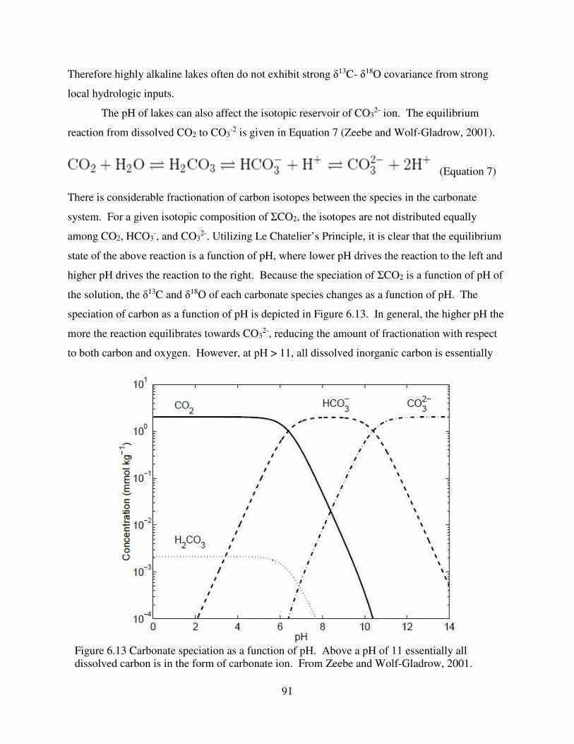
91

Therefore highly alkaline lakes often do not exhibit strong δ13C- δ18O covariance from strong

local hydrologic inputs.

The pH of lakes can also affect the isotopic reservoir of CO32- ion. The equilibrium

reaction from dissolved CO2 to CO3-2 is given in Equation 7 (Zeebe and Wolf-Gladrow, 2001).

(Equation 7)

There is considerable fractionation of carbon isotopes between the species in the carbonate

system. For a given isotopic composition of ΣCO2, the isotopes are not distributed equally

among CO2, HCO3-, and CO3

2-. Utilizing Le Chatelier’s Principle, it is clear that the equilibrium

state of the above reaction is a function of pH, where lower pH drives the reaction to the left and

higher pH drives the reaction to the right. Because the speciation of ΣCO2 is a function of pH of

the solution, the δ13C and δ18O of each carbonate species changes as a function of pH. The

speciation of carbon as a function of pH is depicted in Figure 6.13. In general, the higher pH the

more the reaction equilibrates towards CO32-, reducing the amount of fractionation with respect

to both carbon and oxygen. However, at pH > 11, all dissolved inorganic carbon is essentially

Figure 6.13 Carbonate speciation as a function of pH. Above a pH of 11 essentially all dissolved carbon is in the form of carbonate ion. From Zeebe and Wolf-Gladrow, 2001.

92

CO32-, thus the δ13C of CO3

2- is equal to δ13CΣCO2. A more complete description of how carbon

and oxygen isotopes vary with pH can be found in Zeebe and Wolf-Gladrow, 2001.

Water Chemistry and Mineral Speciation

Stable isotopes were measured for forty-one samples across the measured sections

included in this study. A list of all the stable isotope values accompanied by their facies,

measured section, and calculated weight percent calcite and dolomite from XRF (see section 6.1)

is in Appendix E.

The isotopic controls of δ13C include evaporation-precipitation and organic

photosynthesis/respiration, while the controls on δ18O only include evaporation-precipitation,

therefore δ18O approximates salinity locally better than δ13C. This study plotted the dolomite as

a percent of total carbonate in a sample against the stable isotopes measured (Figure 6.14).

There is a moderate-to-strong correlation between the δ18O and carbonate speciation, while no

correlation between δ13C and carbonate speciation. This corroborates with other studies which

have observed that dolomite precipitation is facilitated by elevated salinities (e.g. Van Lith et al.

2002). Dolomite consistently contains elevated δ13C and δ18O values relative to calcite as a

result of preferentially precipitating in saline waters enriched in 13C and 18O.

Isotopic Stratigraphy in the Carbonate Marker Unit

The δ13C and δ18O of carbonates sampled in the CMU at the Highway 191 roadcut and

Nine Mile Canyon were plotted adjacent to the measured section, facies association, and

transgressive-regressive cycles. The results are shown in Figure 6.15.

The Highway 191 roadcut section exhibits strong δ13C- δ18O covariance. At the base of

the CMB, δ18O diverges from δ13C and is enriched with respect to 18O. This is the result of

deepening of the lake and passing beneath the chemocline where salinity is elevated.

Consequently, there was an increase in the precipitation of dolomite or protodolomite relative to

calcite, changing the fractionation factor of mineralization. This can be demonstrated in figure

6.14 where there is a strong correlation between δ18O and percent carbonate that is dolomite.

Additionally, it is possible that the increased total dissolved solids beneath the chemocline can

lower the pH of the water as a result of concentrating electron acceptor Lewis acids such as Na+,

Mg2+, Fe2+, and Fe3+. Reducing the pH of the water increases the fractionation of carbon in

93

Figure 6.14 Depicts the correlation between δ13C and δ18O and the mineral speciation of carbonate. There is a moderate-to-strong correlation between δ18O and the precipitation of dolomite and no correlation between δ13C and the precipitation of dolomite.

94

Figure 6.15 Shows the δ13C and δ18O of the Carbonate Marker Unit in both the Highway 191 roadcut and Nine Mile Canyon. The Highway 191 roadcut exhibits strong isotopic covariance while the Nine Mile Canyon outcrop exhibits weak covariance.

95

equilibrium from dissolved CO2 to CO3-2 as discussed above, this in turn depletes precipitated

carbonate with respect to 13C. Both of these principles are capable of creating a minor divergence

of carbon and oxygen isotope values in a highly stratified lake when deposition crosses beneath

the chemocline. The δ13C and δ18O are isotopically heavy at the baseof the section at

approximately 10‰ and 1‰, respectively, and gradually lighten up through the stratigraphy

ending at approximately 1 δ13C‰ and -4 δ18O‰, respectively. A freshwater pulse at the top of

the CMB is denoted by a dramatic depletion of δ18O, denoting the onset of the fluvial Renegade

Tongue Member. There is also observed a minor depletion of δ13C, but it is reduced as a result

of alkalinity buffering described above.

The Nine Mile Canyon section exhibits weak δ13C-δ18O covariance. Oxygen fluctuates

repeatedly between -1 and -8 δ18O‰, but most commonly is observed most enriched in 18O in

association with shoal complex deposits and most depleted in 18O in association with deltaic

deposits. When the fluvial axis was aligned with Nine Mile Canyon, fresh water locally reduced

the salinity and created local nearshore zones of isotopically light oxygen. However, because the

alkalinity in the lake is much greater than the alkalinity of input waters, carbon was well-

buffered with respect to δ13C in the lake. As a result, carbon values show a steady enrichment

with respect to 13C starting at approximately -11 δ13C‰ and ending at approximately 0 δ13C‰

and does not covary with oxygen. Isotopically light ground waters and river waters generally

having low δ13C, and produce values for calcite precipitates between -10‰ and -15‰ (Leng and

Marshall 2004).

The δ13C values at the Highway 191 roadcut start isotopically heavy and gradually get

lighter up section, while the δ13C values at the Nine Mile Canyon start isotopically light and

gradually get heavy up section. By the top of the CMB both measured sections isotopic values

have reached nearly identical values at approximately 1 δ13C‰. The Highway 191 roadcut near

the base is enriched with respect to δ13C as a result of respiration and photosynthesis, denoted by

the abundance of molluscs, ostracod, and coals in this stratigraphic interval. Additionally, high

amounts of mudflat evaporation elevated both δ13C and δ18O. As the lake deepened and the

deposits got farther from the high evaporation mudflat environment, the overall profile of the

measured section freshened and became less organically productive. Nine Mile Canyon,

however, was closely aligned with the fluvial freshwater axis at the time. An abundance of

isotopically light carbon from deltaic deposits and hydrologic input locally depleted the lake with

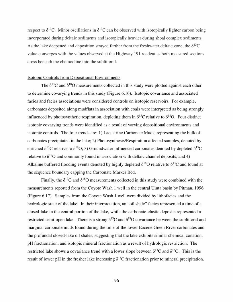
96

respect to δ13C. Minor oscillations in δ13C can be observed with isotopically lighter carbon being

incorporated during deltaic sediments and isotopically heavier during shoal complex sediments.

As the lake deepened and deposition strayed farther from the freshwater deltaic zone, the δ13C

value converges with the values observed at the Highway 191 roadcut as both measured sections

cross beneath the chemocline into the sublittoral.

Isotopic Controls from Depositional Environments

The δ13C and δ18O measurements collected in this study were plotted against each other

to determine covarying trends in this study (Figure 6.16). Isotopic covariance and associated

facies and facies associations were considered controls on isotopic reservoirs. For example,

carbonates deposited along mudflats in association with coals were interpreted as being strongly

influenced by photosynthetic respiration, depleting them in δ13C relative to δ18O. Four distinct

isotopic covarying trends were identified as a result of varying depositional environments and

isotopic controls. The four trends are: 1) Lacustrine Carbonate Muds, representing the bulk of

carbonates precipitated in the lake; 2) Photosynthesis/Respiration affected samples, denoted by

enriched δ13C relative to δ18O; 3) Groundwater influenced carbonates denoted by depleted δ13C

relative to δ18O and commonly found in association with deltaic channel deposits; and 4)

Alkaline buffered flooding events denoted by highly depleted δ18O relative to δ13C and found at

the sequence boundary capping the Carbonate Marker Bed.

Finally, the δ13C and δ18O measurements collected in this study were combined with the

measurements reported from the Coyote Wash 1 well in the central Uinta basin by Pitman, 1996

(Figure 6.17). Samples from the Coyote Wash 1 well were divided by lithofacies and the

hydrologic state of the lake. In their interpretation, an “oil shale” facies represented a time of a

closed-lake in the central portion of the lake, while the carbonate-clastic deposits represented a

restricted semi-open lake. There is a strong δ13C and δ18O covariance between the sublittoral and

marginal carbonate muds found during the time of the lower Eocene Green River carbonates and

the profundal closed-lake oil shales, suggesting that the lake exhibits similar chemical zonation,

pH fractionation, and isotopic mineral fractionation as a result of hydrologic restriction. The

restricted lake shows a covariance trend with a lower slope between δ13C and δ18O. This is the

result of lower pH in the fresher lake increasing δ13C fractionation prior to mineral precipitation.

97

Figure 6.16 Depicts covarying trends of δ13C and δ18O with respect to depositional environment and controls from samples measured in this study.

98

Figure 6.17 Depicts covarying trends of δ13C and δ18O with respect to depositional environment and controls from samples measured in this study and taken from the Coyote Wash 1 well analyzed in Pitman, 1996. This study finds that Pitman Primary trend and Pitman Diagenetic trend may instead be a relic of depositional pH and differential carbon fractionation in high pH systems.

99

CHAPTER 7

DISCUSSION

Lakes are commonly classified into one of three groups: underfilled, balance filled, or

overfilled depending on the rate of hydrologic inflow relative to the rate of potential

accommodation (Bohacs et al. 2000). Overfilled lakes have rates of sediment and hydrologic

input that exceeds the production of accommodation space, commonly resulting in a freshwater,

open lacustrine system. Underfilled lakes have low rates of accommodation that result from low

inflow or net evaporation of water and low sediment fill, commonly resulting in high salinities,

and low biodiversity. Balance-filled lakes are intermediate in water inflow, sediment supply, and

accommodation rates. Both progradational and aggradational stacking patterns are the result of

highly oscillatory lake levels, commonly alternating between freshwater open and saline closed

drainage system. During the Carbonate Marker Unit and D Marker Units, ancient Lake Uinta

was a balance-filled lake with water level fluctuations that reflected the monsoon-style

seasonality of the Eocene (Plink-Björklund and Birgenheier 2012).

7.1 Paleo-Lake Uinta during the Lower Eocene

The Carbonate Marker Unit is a thick deltaic-lacustrine lake highstand during the lower

Eocene Green River Formation. Five cycles are identified in the Carbonate Marker Unit, three

cycles during a rapidly fluctuating lake and two cycles within a gradually fluctuating lake.

Two freshwater periods in the lake are observed in the Carbonate Marker Unit. The first

is during the basal three cycles of the rapidly fluctuating lake and the expansion of ancient Lake

Uinta within the Green River Formation. This freshwater transition is denoted by the presence of

molluscs, coals, and ostracod blooms. As discussed previously, molluscs require relatively

freshwater conditions to survive, while coals require broad freshwater swamps in which to

support dense terrigenous plant life. In the basal cycle of the Highway 191 roadcut, tens of

meters of fine-grained siliciclastics containing large bivalve and gastropod tests are the result of

siliciclastic retrogradation and filling of the lake with fluvial-derived freshwater. Additionally, in

the Highway 191 roadcut and in Nine Mile Canyon coals are observed in all three of the basal

rapidly fluctuating lake cycles, suggesting broad freshwater swamps along the lake margin that

were capable of supporting abundant plant life. Finally, although ostracods are observed in the

100

lake throughout the Carbonate Marker Unit, the absence of ostracod tests within the sublittoral

carbonate mudstones suggests that ostracods prefer living along the freshwater, nutrient rich

lacustrine margins. During freshwater periods and hydrologic input and deltaic derived nutrient

levels were high, ostracod blooms were common, depositing thick packages of argillaceous

ostracod wackestones and ostracod claystones (F3.1).

The second period of freshwater input occurred during the transgression of the second

gradually fluctuating lake cycle. Evidence for lake freshness is found in the transition from shoal

complex to sublittoral deposits in the Highway 191 roadcut and Nine Mile Canyon beneath the

Carbonate Marker Bed and the resurgence of gastropod and bivalve biota, clay-rich ostracod

blooms, and the addition of fish bone fragments. Although fish fragments do not directly

correspond to salinity, the absence of fish bones both above and below the second salinity zone

may indicate limited abundance and stressful lake conditions. Coal was observed at this time at

the Hay Canyon outcrop, further supporting the idea of freshwater lacustrine margins hospitable

to life. Finally, ostracod blooms and flood cycles were also common during the transgression and

onset of the Carbonate Marker Bed, indicating sediment rich floods which brought in nutrients

and clays and freshened the lake. One hypothesis is that Lake Uinta and Lake Piceance were

hydrologically connected during the Carbonate Marker Bed, allowing for the migration of fish

over the Douglas Creek Arch. Further stratigraphic analysis of this formation to the east is

required to test this hypothesis.

The Carbonate Marker Bed is a sublittoral 20 to 30 meter thick dolomitic lime mudstone

with variable amounts of organic matter. The bed exhibits the most basinward lacustrine facies

observed in this study and is the deepest lake over the interval studied. Limited bioturbation and

inconsistent preservation potential of organic matter indicate that the lake bottom was

periodically exposed to oxygenated waters during storm events. However, during most of the

Carbonate Marker Bed the lake bottom contained a well-defined chemocline. Above the

chemocline in the mixolimnion waters were well-oxygenated, relatively fresh, moderately

alkaline, and highly productive. During the freshwater zones described above, littoral deposits

are not observed containing analcime and dolomite precipitation is minimal, further suggesting

reduced salinity within the well-mixed mixolimnion portion of the lake. However, freshwater

periods retained a well-developed chemocline with elevated salinity, high pH, low eH, and

anoxia to dysoxia in the monimolimnion layer beneath the chemocline. This is evident by the

101

presence of authigenic analcime, ferroan dolomite, and alteration of clay species within

sublittoral sediments.

Between the two freshwater events noted above, elevated salinities likely excluded

primary grazer taxa such as gastropods, and as a result, there was elevated microbial activity and

preservation within the lake. High-energy grainstones deposited within shoals are commonly

coated by dolomitic oncolitic fabrics that were produced from microbial activity. However, the

lake was commonly exposed to episodic freshening and under-saturation with respect to

dolomite, resulting in micritization and dissolution of many oncolitic grains and replacement

with calcite micrite or spar.

Overall, the Carbonate Marker Unit is a transgressive lacustrine unit that is capped by a

rapid regression that marks the onset of the fluvio-deltaic Renegade Tongue sandy member of

the Sunnyside Delta. This rapid regression is a sequence boundary and is the datum for the

sections measured in this study. The Renegade Tongue Member is capped by a regionally

correlative lake transgression known as the D Marker Unit. Despite the stratigraphic dip across

the section, the D Marker Unit has a relatively consistent thickness in all three measured

sections, indicating a rapid transgression that flooded the lake margin simultaneously. The lake

during DMU time was more saline than the CMU resulting in well-developed microbialites,

fewer ostracods, and essentially no molluscs or fish bones.

Isotopic analysis of the Carbonate Marker Unit at the Highway 191 roadcut and the Nine

Mile Canyon outcrops show that the lake was very poorly mixed with respect to vertical and

lateral zonation. The monsoon style episodic style of flooding likely contributed to keeping the

lake highly stratified vertically. Near the fluvial axis at Nine Mile Canyon, fresh input waters

locally depleted carbonate deposition with respect to 13C and 18O and in some cases precipitating

carbonate with very light δ13C from ground waters. As Nine Mile Canyon alternated between

shoal dominated and delta dominated, dramatic fluctuations in δ18O can be observed, however,

because the lake was highly alkaline, the δ13C remained buffered and shows only minor

variations.

At the Highway 191 roadcut there was strong covariance between δ13C and δ18O,

indicating that evaporation and precipitation were the primary controls on the isotopic reservoir

of carbon. However, near the base of the section, increased photosynthesis and respiration

locally enriched carbonate with respect to δ13C. As the lake deepened the waters became overall

102

fresher and depleting the lake with respect to δ13C and δ18O. By the Carbonate Marker Bed, both

the Highway 191 roadcut and Nine Mile Canyon measured sections were far enough away from

the lake shoreline to experience the micro-environmental controls found lower in the sections.

Beneath the chemocline in the sublittoral, the δ13C from both the Highway 191 roadcut and Nine

Mile Canyon approached approximately 0-1‰, indicating that their depositional environments

have become similar and isolated from the coastal microenvironments. The Carbonate Marker

Bed is capped by an alkaline buffered flooding event denoted by a highly depleted δ18O value

relative to δ13C, designating the onset of the Renegade Tongue and a sequence boundary.

7.2 Modern Analogs

Several attributes of ancient Lake Uinta at the time of the Carbonate Marker Unit and D

Marker Unit can be observed in modern lacustrine systems. The most pronounced physical,

biological, and chemical properties of ancient Lake Uinta include a closed-lake, low angle ramp-

style bathymetry, shorelines with highly variable lithology including both mudflats and ooid

shoals, high siliciclastic influx into the lake that can build deltas, a well-developed chemocline

that does not turn over seasonally, and high total dissolved solids with relative depletion of

calcium and magnesium relative to sodium. The exact parameters for each of these systems is

not well-understood in the rock record, but similar characteristics can be found individually in

modern analogs around the world.

Asymmetric closed-lakes are common in tectonic compressional regimes, however ramp

style bathymetry is common. Ramp margins are conducive to a wide variety of marginal

depositional environments, including both high energy ooid shoals and low energy mudflats.

Examples of highly variable ramp margin lakes include Pyramid Lake, Nevada (Popp and

Wilkinson 1983) and the Great Salt Lake, Utah. Modern analogs for siliciclastic input

comparable to an Eocene time fluvial megafan is unclear, however lakes with high siliclastic

sediment input that build extensive lacustrine deltas do exist today. One such example of a

balanced-lake that has a shoreline sensitive to climatic forcing is Lake Hayk, Ethiopia (Ghinassi

et al. 2015).

Alkalinity in Lake Uinta was elevated relative to modern analogs by the high pCO2 in the

atmosphere. Elevated alkalinity and pH comparable to ancient Lake Uinta can be found in lakes

such as the Big Soda Lake, Nevada (Kharaka et al. 1984) and Mono Lake, California.

103

Additionally, Big Soda Lake, Nevada contains high total dissolved solids elevated with respect

to sodium. Finally, ancient Lake Uinta had a well-developed chemocline that did not appear to

mix seasonally or turn over during summer floods. This is likely the result of monsoon-style

episodic hydrologic input. One such modern lake that has a maximum mixing zone above the

lake-bottom is the deep African rift-lake Lake Malawi, Mozambique and Tanzania (Spigel and

Coulter 1996; Branchu et al. 2005).

104

CHAPTER 8

CONCLUSIONS

Based on analyses of the Carbonate Marker and D Marker units in outcrop, thin section,

X-ray fluorescence, X-ray diffraction, QEMSCAN, and stable isotopes, conclusions of this study

include the following:

1. Rocks in the Carbonate Marker Unit and D Marker Unit are divided into five families

based on lithologic composition. These are: (1) Sandstones; (2) Grain-Rich limestones

including packstones, grainstones, floatstones, and rudstones; (3) Bioclastic claystones

and siltstones; (4) Unfossiliferous claystones and siltstones; and (5) Carbonate mudstones

composed of either calcite or dolomite.

2. Facies within this study occur in four distinct facies associations: (1) Delta; (2) Mudflat;

(3) Shoal Complex; and (4) Sublittoral.

3. Transgressive-regressive lake cycles were identified within the Carbonate Marker Unit in

two distinct styles characterized by either rapidly fluctuating lake levels or gradually

fluctuating lake levels. Rapidly fluctuating lakes show slow regressions followed by rapid

flooding, while gradually fluctuating lakes show both slow transgressions and

regressions.

4. Five transgressive-regressive cycles were identified within the Carbonate Marker Unit.

The basal three cycles were in a rapidly fluctuating lake, while the upper two were in a

gradually fluctuating lake. Because of the dip component and gradual transgression of the

lake during the Carbonate Marker Unit, the basal cycle onlapped onto the Colton Tongue

between the Highway 191 roadcut and the Nine Mile Canyon outcrop, and the two upper

cycles of the rapidly fluctuating lake onlapped onto the Colton Tongue between the Nine

Mile Canyon outcrop and the Hay Canyon outcrop.

5. At the top of the Carbonate Marker Unit in both the Highway 191 roadcut and Nine Mile

Canyon is the Carbonate Marker Bed, a 20 to 30 meter thick sublittoral carbonate

mudstone that represents the deepest lake over the stratigraphic interval studied. The

Carbonate Marker Bed is capped by the fluvio-deltaic sandy pulse of the Renegade

105

Tongue. The boundary between the Carbonate Marker Bed and the Renegade Tongue is a

rapid regression and a sequence boundary.

6. Excluding the Carbonate Marker Bed, Nine Mile Canyon is dominated by deltaic and

shoal facies, the Highway 191 roadcut is dominated by mudflat and shoal facies. Hay

Canyon contains both deltaic and shoal facies, but based on limited petrographic

evidence, it is hypothesized that the sediment source for Hay Canyon is different from the

sediment source for Nine Mile Canyon and the Highway 191 roadcut.

7. The D Marker Unit is a two to four meter carbonate unit that is laterally correlative

between the studied sections and separates the Renegade Tongue from the Sunnyside

Delta. Despite the stratigraphic dip across the section, the D Marker Unit has a consistent

thickness in all three study areas, indicating a rapid transgression that flooded all three

sections simultaneously. The lake during DMU time was more saline than the CMU

resulting in well-developed microbialites, fewer ostracods, and essentially no molluscs or

fish bones.

8. Carbonate mudstones show elevated high weight percent silicate relative to grain rich

carbonates, both as the result of calm waters and high preservation potential of fine-

grained clays, and as the result of analcime precipitation within hypersaline environments

along mudflats and in the sublittoral where carbonate muds are preserved.

9. Oolitic and oncolitic coating of grains is generally composed of dolomite, but commonly

undergoes early micritization and dissolution that is replaced with calcite micrite or spar.

Dolomitic mud in the sublittoral is most often preserved within the sheltered

microenvironment of articulated ostracod tests.

10. Gamma-ray values were calculated for each facies observed and plotted to demonstrate

statistical spread and outliers. Claystones and siltstones exhibited the highest standard

deviation among the facies observed, while carbonate mudstones and packstones were

consistently clean. Sandstones were consistently observed with high gamma-ray

response, averaging between 80 to 180 API units due to high uranium and thorium

measurements in XRF.

11. There is a strong correlation between δ18O and the percent of carbonate that precipitates

as dolomite, and there is no correlation between δ13C and the percent of carbonate that

precipitates as dolomite. Since δ18O more accurately reflects changes in salinity while

106

δ13C reflects changes in organic productivity, total alkalinity, and pH, it can be observed

that dolomite is most strongly controlled by salinity in Lake Uinta at the time of this

study.

12. There is strong covariance with respect to carbonates in the lake, indicating that the lake

was a closed-lake and hydrologically restricted. Additionally, microenvironments along

margin of the lake created localized conditions that differ from the overall lake. These

include: 1) zones of high photosynthesis/respiration in coastal swamps found at the base

of the Highway 191 roadcut; 2) zones of groundwater precipitated carbonates found at

the base of the Nine Mile Canyon outcrop; and 3) a freshwater pulse buffered by high

lake alkalinity that denotes the onset of the Renegade Tongue and a sequence boundary.

These microenvironments further corroborate that the lake was poorly mixed both

vertically and laterally during the lower Eocene.

13. The isotopic measurements of lacustrine carbonates, excluding the microenvironments

mentioned above, show a strong correlation with previous research measuring the closed-

lake oil-shale facies found basinward in the lake. Carbonates deposited during the closed-

lake are less fractionated with respect to δ13C than carbonates precipitated during the

restricted semi-open lake, suggesting higher pH during hydrologically restricted times.

14. Ancient Lake Uinta was a stratified lake with a well-developed chemocline, most likely

the result of the monsoon style episodic flooding of input waters. Above the chemocline

in the mixolimnion waters were well-oxygenated, moderately saline, moderately alkaline,

and highly productive. Below the chemocline in the monimolimnion dense highly saline

waters were anoxic or dysoxic, high pH, and low eH. The following observations are the

result of a well-stratified lake:

• Clay speciation is reduced upon entering the lake by alteration and dissolution. A

full suite of detrital chlorite, smectite, illite, and kaolinite was observed in delta

floodplain sediments whereas a sample from the shallow lake showed only illite,

kaolinite, and minor smectite. A sample taken from the sublittoral/profundal lake

environment contained only illite.

• Rocks deposited in the monimolimnion commonly are composed of ferroan

dolomite. This is the result of low eH conditions which reduce Fe3+ to Fe2+ such

107

that it substitutes for magnesium in dolomite. Ferroan dolomite can cause

significant damage to acid hydraulic fracture techniques if not properly managed.

• Authigenic analcime is found throughout all portions of the lake as pore-filling

cement, however it is most pronounced in the sublittoral where it is commonly

found replacing carbonate mud.

108

REFERENCES CITED

Andrews, Anthony. 2006. Oil Shale: History, Incentives, and Policy. Washington D.C.

Bohacs, Kevin M, Alan R Carroll, and Jack E Neal. 2003. “Lessons from Large Lake Systems — Thresholds, Nonlinearity, and Strange Attractors.” Special Papers-Geologic Society of

America 370: 75–90.

Bohacs, Kevin M. 2001. Basin Evolution of the Green River Formation in the Uinta and

Washakie Basins : Insights for Lacustrine Hydrocarbon Systems. AAPG 2001 Post-Meeting

Field Trip.

Bohacs, Kevin M., Alan R. Carroll, John E. Neal, and Paul J. Mankiewicz. 2000. “Lake-Basin Type, Source Potential, and Hydrocarbon Character: An Integrated Sequence-Stratigraphic-Geochemical Framework.” Edited by Elizabeth H. Gierlowski-Kordesch and Kerry R. Kelts. AAPG Studies in Geology 46. The American Association of Petroleum Geologists: 3–34.

Branchu, Philippe, Laurent Bergonzini, Damien Delvaux, Marc De Batist, Vladimir Golubev, Marc Benedetti, and Jean Klerkx. 2005. “Tectonic, Climatic and Hydrothermal Control on Sedimentation and Water Chemistry of Northern Lake Malawi (Nyasa), Tanzania.” Journal

of African Earth Sciences 43 (4): 433–46. doi:10.1016/j.jafrearsci.2005.09.004.

Breheret, J.G., A. Fourmont, J. J. Macaire, and P. Negrel. 2008. “Microbially Mediated Carbonates in the Holocene Deposits from Sarlieve, a Small Ancient Lake of Hte French Massif Central, Testify to the Evolution of a Restricted Environment.” Sedimentology 55 (3): 557–78.

Buchheim, H.P, L.R Brand, and H.T Goodwin. 2000. “Lacustrine to Fluvial Floodplain Deposition in the Eocene Bridger Formation.” Palaeogeography, Palaeoclimatology,

Palaeoecology 162 (1): 191–209.

Carroll, Alan R., Lauren M. Chetel, and M. E. Smith. 2006. “Feast to Famine: Sediment Supply Control on Laramide Basin Fill.” Geology 34 (3): 197.

Cashion, W B. 1995. “Stratigraphy of the Green River Formation, Eastern Uinta Basin, Utah and Colorado-A Summary.” The Green River Formation in Piceance Creek and Eastern Uinta

Basin Field Trip, 15–21.

Castanier, Sabine, Gaele Le Metayer-Levrel, and Jean-Pierre Perthuisot. 1999. “Ca-Carbonates Precipitation and Limestone Genesis — the Microbiogeologist Point of View.” Sedimentary

Geology 126 (1): 9–23.

Clementz, Mark T, and Jacob O Sewall. 2011. “Latitudinal Gradients in Greenhouse Seawater δ18O: Evidence from Eocene Sirenian Tooth Enamel.” Science 332 (6028): 455–58.

109

Cole, R. D., and M. D. Picard. 1978. “Comparative Mineralogy of Nearshore and Offshore Lacustrine Lithofacies, Parachute Creek Member of the Gren River Formation, Piceance Creek Basin, Colorado, and Eastern Uinta Basin, Utah.” Geological Society of America

Bulletin.

Craig, Harmon. 1957. “Isotopic Standards for Carbon and Oxygen and Correction Factors for Mass-Spectrometric Analysis of Carbon Dioxide.” Geochimica et Cosmochimica Acta 12 (1-2): 133–49.

Davaud, E., and Girardclos. 2001. “Recent Freshwater Ooids and Oncoids from Western Lake Geneva (Switzerland): Indications of a Common Organically-Mediated Origin.” Journal of

Sedimentary Research 71: 423–29.

Davis, S. J., H. T. Mix, B. a. Wiegand, a. R. Carroll, and C. P. Chamberlain. 2009. “Synorogenic Evolution of Large-Scale Drainage Patterns: Isotope Paleohydrology of Sequential Laramide Basins.” American Journal of Science 309 (7): 549–602.

Davis, Steven J., Andreas Mulch, Alan R. Carroll, Travis W. Horton, and C. Page Chamberlain. 2009. “Paleogene Landscape Evolution of the Central North American Cordillera: Developing Topography and Hydrology in the Laramide Foreland.” Geological Society of

America Bulletin 121 (1-2): 100–116.

DeCelles, P. G., and J. C. Coogan. 2006. “Regional Structure and Kinematic History of the Sevier Fold-and-Thrust Belt, Central Utah.” Geological Society of America Bulletin 118 (7-8): 841–64.

DeCelles, Peter G. 1994. “Late Cretaceous-Paleocene Synorogenic Sedimentation and Kinematic History of Hte Sevier Thrust Belt, Northeast Utah and Southwest Wyoming.” Geological

Society of America Bulletin 106 (1): 32–56.

Dickinson, William R., Margaret A. Klute, Michael J. Hayes, Susanne U. Janecke, Erik R. Lundin, Mary A. McKittrick, and Mark D. Olivares. 1988. “Paleogeographic and Paleotectonic Setting of Laramide Sedimentary Basins in the Central Rocky Mountain Region.” Geological Society of America Bulletin 100 (7). Geological Society of America Bulletin: 1023–39.

Fouch, Thomas d., W. B. Cashion, Robert T. Ryder, and J. H. Campbell. 1976. “Field Guide to Lacustrine and Related Nonmarine Depositional Environments in Tertiary Rocks, Uinta Basin, Utah.” In Studies in Colorado Field Geology, edited by Rudy C. Epis and Robert J. Weimer, 27.

Franczyk, K.J., J.K. Pitman, W.B. Cashion, J.R. Dyni, T.D. Fouch, R.C. Johnson, M.A. Chan, J.R. Donnell, T.F. Lawton, and R.R. Remy. 1989. “Evolution of Resource-Rich Foreland and Intermontane Basins in Eastern Utah and Western Colorado.” In Internation Geological

Congress Field Trip Guidebook T-324, 53. American Geophysical Union.

110

Ghinassi, Massimiliano, Filippo D’Oriano, Marco Benvenuti, Mariaelena Fedi, and Stanley Awramik. 2015. “Lacustrine Facies in Response to Millennial-Century Scale Climate Changes (Lake Hayk, Northern Ethiopia).” Journal of Sedimentary Research 85 (4): 381–98.

Gierlowski-Kordesch, Elizabeth H. 2010. “Carbonates in Continental Settings: Facies, Environments, and Processes.” In Develpment in Sedimentology Volume 61, edited by A M Alonso-Zarza and L H Tanner, 62:378. Developments in Sedimentology. Amsterdam, The Netherlands: Elsevier.

Hanley, J. H., T. D. Fouch, G. E. Claypool, and R. H. Tschudy. 1976. “Paleontology, Geochemistry, and Depositional Environments of Some Lower Tertiary Coals, North-Central Utah--Implications for Detection of Contential Petroleum Source-Rocks.” In Annual

Meeting of the Geological Society of America Abstracts with Programs, 902.

Johnson, R.C. 1985. “Early Cenozoic History of the Uinta and Piceance Creek Basins, Utah and Colorado, with Special Reference to the Development of Eocene Lake Uinta.” In Cenozoic

Paleogeography of the West-Central United States, edited by R. M. Florres and S. s. Kaplan, 247–76. Rocky Mountain Paleography Symposium 3: The Rocky Mountain Section, Society of Economic Paleontologists and Mineralogists, Denver, CO, 247–276.

Johnson, R.C., T. J. Mercier, and M.E. Brownfield. 2011. “Assessment of In-Place Oil Shale Resources of the Green River Formation , Uinta Basin , Utah and Colorado.” U.S.

Geological Survery Fact Sheet 2011 (3063): 4.

Keighley, David, Stephen Flint, John Howell, and Andrea Moscariello. 2003. “Sequence Stratigraphy in Lacustrine Basins: A Model for Part of the Green River Formation (Eocene), Southwest Uinta Basin, Utah, U.S.A.” Journal of Sedimentary Research 73 (6): 987–1006.

Kharaka, Yousif K., Stephen W. Robinson, Leroy M. Law, and William W. Carothers. 1984. “Hydrogeochemistry of Big Soda Lake, Nevada: An Alkaline Meromictic Desert Lake.” Geochimica et Cosmochimica Acta 48 (4): 823–35.

Lawton, Timothy F. 2008. “Laramide Sedimentary Basins.” In The Sedimentary Basins of the

United States and Canada, edited by Andrew D. Miall and K. J. Hsü, 5:429–50. Sedimentary Basins of the World. Amsterdam, The Netherlands: Elsevier.

Leng, Melanie J., and Jim D. Marshall. 2004. “Palaeoclimate Interpretation of Stable Isotope Data from Lake Sediment Archives.” Quaternary Science Reviews 23 (7-8): 811–31.

Leopold, E. B. 1969. “Late Cenozoic Palynology.” In Aspects of Palynology, edited by R. H. Tschudy and R. A. Scott, 123–34. New York: Wiley-Interscience.

Li, H. C., and T. L. Ku. 1997. “δ13C-δ18O Covariance as a Paleohydrological Indicator for Closed-Basin Lakes.” Palaeogeography, Palaeoclimatology, Palaeoecology 133 (1-2): 69–80.

111

Moncure, George, and Ronald C Surdam. 1980. “Depositional Environment of the Green River Formation in the Vicinity of the Douglas Creek Arch , Colorado and Utah.” Rocky

Mountain Geology 19 (1): 9–24.

Moore, D.M., and R.C. Reynolds. 1997. X-Ray Diffraction and the Identification and Analysis of

Clay Minerals. 2nd Ed. Oxford University Press.

Olariu, Cornel, Janok P. Bhattacharya, Matthew I. Leybourne, Stephen K. Boss, and Robert J. Stern. 2012. “Interplay between River Discharge and Topography of the Basin Floor in a Hyperpycnal Lacustrine Delta.” Sedimentology 59 (2): 704–28.

Osmond, John C. 1965. “Geologic History of Site of Uinta Basin, Utah” 49 (11).

Perlmutter, M.A., and M. D. Matthews. 1992. “Global Cyclostratigraphy.” In Quantitative

Dynamic Stratigraphy, 223–60. Argonne National Laboratory, University of Chicago.

Picard, M. D. 1963. “Duration of Eocene Lake, Uinta Basin, Utah.” Geological Society of

America Bulletin 74: 89–90.

Picard, M. Dane, and Lee R. High. 1972. “Paleoenvironmental Reconstructions in an Area of Rapid Facies Change, Parachute Creek Member of Green River Formation (eocene), Uinta Basin, Utah.” Bulletin of the Geological Society of America 83 (9): 2689–2708.

Picard, M.D. 1985. “Hypothesis of Oil-Shale Genesis, Green River Formation, Northeast Utha, Northwest Colorado, and Southwest Wyoming.” In Geology and Energy Resources, Uinta

Basin of Utah. Salt Lake City, Utah.

Pitman, Janet K. 1996. Origin of Primary and Diagenetic Carbonates in the Lacustrine Green

River Formation (Eocene), Colorado and Utah. U.S. Geological Survey Bulletin.

Platt, N. H., and V. P. Wright. 1991. “Lacustrine Carbonates: Facies Models, Facies Distributions and Hydrocarbon Aspects.” Special Publications of the International

Association of Sedimentologists, no. 13: 57–74.

Plink-Björklund, Piret, and Lauren Birgenheier. 2012. “Extreme Seasonality during Early Eocene Hyperthermals.” AGU Fall Meeting Abstracts 1: 1005.

Popp, B. N., and B. H. Wilkinson. 1983. “Holocene Lacustrine Ooids from Pyramid Lake, Nevada.” In Coated Grains, edited by T. M. Peryt, 142–53. Springer.

Remy, Robert R. 1985. “Distribution and Origin of Analcime in Marginal Lacustrine Mudstones of the Green River Formation, South-Central Uinta Basin, Utah.” Clays and Clay Minerals 37 (5): 419–32.

112

———. 1992. Stratigraphy of the Eocene Part of the Green River Formation in the South-

Central Part of the Uinta Basin, Utah. U.S. Geological Survey Bulletin. Vol. 1787. Washington: United States Government Printing Office.

Renaut, Robin W., and Elizabeth H. Gierlowski-Kordesch. 2010. “Lakes.” In Facies Models, edited by Noel P. James and Robert W. Dalrymple, 4th ed., 541–75. Toronto: Geological Association of Canada.

Roehler, Henry W. 1993. Eocene Climates, Depositional Environments, and Geography, Greater

Green River Basin, Wyoming, Utah, and Colorado. Geology of the Eocene Wasatch, Green

River, and Bridger (Washakie) Formations, Greater Green River Basin, Wyoming, Utah,

and Colorado. Washington: United States Government Printing Office.

Ruble, Tim E, M. D. Lewan, and R. P. Philp. 2001. “New Insights on the Green River Petroleum System in the Uinta Basin from Hydrous Pyrolysis Experiments.” AAPG Bulletin 85 (8): 1333–71.

Ryder, Robert T., Thomas d. Fouch, and James H. Elison. 1976. “Early Tertiary Sedimentation in the Western Uinta Basin, Utah.” Geological Society of America Bulletin 87 (4): 496–512.

Sanz-Montero, M.E., J. P. Rodriguez-Aranda, and Jose P Calvo. 2006. “Mediation of Endoevaporitic Microbial Communities in Early Replacement of Gypsum by Dolomite: A Case Study from Miocene Lake Deposits from the Madrid Basin, Spain.” Journal of

Sedimentary Research 76 (12): 1257–66.

Schomacker, Edwin Robert, Audun Vestheim Kjemperud, Johan Petter Nystuen, and Jens Sigurd Jahren. 2010. “Recognition and Significance of Sharp-Based Mouth-Bar Deposits in the Eocene Green River Formation, Uinta Basin, Utah.” Sedimentology 57 (4): 1069–87.

Smith, M. E., K. R. Chamberlain, B. S. Singer, and a. R. Carroll. 2010. “Eocene Clocks Agree: Coeval 40Ar/39Ar, U-Pb, and Astronomical Ages from the Green River Formation.” Geology 38 (6): 527–30.

Spigel, R. H., and G. W. Coulter. 1996. “Comparison of Hydrology and Physical Limnology of the East African Great Lakes: Tanganyika, Malawi, Victoria, Kivu and Turkana (with Reference to Some North American Great Lakes).” In The Limnology, Climatology and

Paleoclimatology of the East African Lakes, edited by T. C Johnson and E. O. Odada, 665. Amsterdam, The Netherlands: Gordon and Breach Science Publishers SA.

Swierenga, Michael. 2014. “Depositional History and Lateral Variability of Microbial Carbonates, Three Mile Canyon and Evacuation Creek, Eastern Uinta Basin, Utah.” Colorado School of Mines.

Talbot, M. R., and P. A. Allen. 1996. “Lakes.” In Sedimentary Environments: Processes, Facies

and Stratigraphy, edited by H.G. Reading, 3rd ed., 83–124. Oxford: Blackwell.

113

Talbot, M.R. 1990. “A Review of the Palaeohydrological Interpretation of Carbon and Oxygen Isotopic Ratios in Primary Lacustrine Carbonates.” Chemical Geology: Isotope Geoscience

Section 80 (4): 261–79.

Tänavsuu-Milkeviciene, Kati, and F. J. Sarg. 2012. “Evolution of an Organic-Rich Lake Basin - Stratigraphy, Climate and Tectonics: Piceance Creek Basin, Eocene Green River Formation.” Sedimentology 59 (6): 1735–68.

Van Lith, Y., C. Vasconcelos, R. Warthmann, J. C F Martins, and J. a. McKenzie. 2002. “Bacterial Sulfate Reduction and Salinity: Two Controls on Dolomite Precipitation in Lagoa Vermelha and Brejo Do Espinho (Brazil).” Hydrobiologia 485 (287): 35–49.

Williamson, Charles R., and M Dane Picard. 1974. “Petrology of Carbonate Rocks in the Green River Formation (Eocene).” Journal of Sedimentary Research 4 (3): 738–59.

Zeebe, R. E., and D. A. Wolf-Gladrow. 2001. “Stable Isotope Fractionation.” In CO2 in

Seawater: Equilibrium, Kinetics, Isotopes, edited by R. E. Zeebe and D. A. Wolf-Gladrow, Volume 65 , 346. Gulf Professional Publishing.

114

APPENDIX A

DETAILED MEASURED SECTIONS

Figure A.1 Facies key. In siliciclastics are colored to indicates sedimentary structure. In carbonates, the color represents the dominant grain type. Additional grains can be added to fully describe the sample. Pattern fills are used to express presence of dolomite, clay, and sand in a carbonate unit.

Sample Taken

Thin Section Made *

115

Figure A.2 Facies Association Key. The facies associations in this study are broken into four environments: FA1: Deltaic, FA2: Mudflat, FA3: Shoal Complex, and FA4: Sublittoral. These colored interpretations are marked to the side of the measured section.

116

Figure A.3 Measured section of the Carbonate Marker Unit at Highway 191 roadcut.

117

Figure A.4 Measured section of the Carbonate Marker Unit at Highway 191 roadcut continued.

118


119


120


121


122


123


124


125


126


127

Figure A.14 Measured section of the Carbonate Marker Unit at Nine Mile Canyon.

128

Figure A.15 Measured section of the Carbonate Marker Unit at Nine Mile Canyon continued.

129


130


131


132


133


134


135

Figure A.22 Measured section of the Carbonate Marker Unit at Hay Canyon.

136

Figure A.23 Measured section of the Carbonate Marker Unit at Hay Canyon continued.

137


138


139

Figure A.26 Measured section of the D Marker Unit at Highway 191 Roadcut.

140

Figure A.27 Measured section of the D Marker Unit at Nine Mile Canyon.

141

Figure A.28 Measured section of the D Marker Unit at Hay Canyon.

142

APPENDIX B

XRF DATA

Table B.1 XRF measurements of weight percent oxides of major rock forming elements, total calculated weight percent of the rock, and calculated gamma-ray response and organized by facies.

Sample # Facies SiO2 Al2O3 CaO MgO FeS2 Fe2O3 K2O CO2 Wt% total Gamma

7 1.1 47.5 5.3 37.7 0.0 0.3 0.2 1.5 29.6 122.1 20.0

8 1.1 57.3 7.9 27.8 0.8 0.4 1.6 1.5 22.7 119.9 60.0

14 1.1 41.0 5.4 19.0 0.7 0.2 2.4 1.9 15.7 86.2 119.3

16 1.1 38.3 4.1 22.7 1.9 0.1 2.1 1.3 19.9 90.4 150.4

33 1.1 47.1 6.0 30.9 2.6 0.3 0.7 1.2 27.2 116.1 60.7

72 1.1 67.5 8.7 13.7 1.5 0.1 3.6 1.8 12.4 109.3 55.8

74 1.1 59.2 10.8 10.3 2.3 0.2 4.5 2.4 10.7 100.4 65.5

80 1.1 37.4 3.7 44.7 1.5 0.4 0.8 1.2 36.7 126.5 42.2

R14 1.1 67.9 7.9 14.9 1.3 0.2 3.1 1.9 13.1 110.3 122.9

R19 1.1 58.8 8.2 22.8 2.8 1.4 1.0 1.6 20.9 117.5 186.1

R53 1.1 72.3 9.9 10.8 0.9 1.9 2.3 1.9 9.5 109.5 112.8

R54 1.1 54.5 14.2 22.3 3.1 1.7 1.9 2.1 20.8 120.5 55.9

R56 1.1 50.4 6.6 22.5 1.3 0.4 1.6 1.6 19.1 103.5 111.3

R66 1.1 53.8 5.8 18.8 2.0 0.1 2.7 1.8 16.9 101.9 43.3

R8 1.1 30.4 6.6 32.7 3.3 0.1 3.3 1.6 29.2 107.3 44.7

22 1.1 50.2 7.0 23.7 1.7 0.7 0.4 1.1 20.5 105.3 81.8

86 1.1 48.0 4.5 30.9 3.3 0.1 0.4 1.7 27.8 116.7 53.5

19 1.2 43.0 7.8 24.0 5.3 0.5 1.9 1.3 24.6 108.5 40.4

29 1.2 46.0 5.9 30.9 4.6 0.3 2.0 1.3 29.3 120.2 39.1

29 1.2 50.2 6.0 26.6 3.1 0.3 2.0 1.5 24.3 114.1 36.9

71 1.2 52.1 6.9 16.0 1.0 1.0 2.4 1.7 13.6 94.7 51.7

71 1.2 55.2 6.8 15.2 0.8 0.3 2.6 1.8 12.8 95.4 59.7

75 1.2 60.1 10.4 6.9 1.6 0.1 3.0 2.5 7.1 91.7 92.8

77 1.2 34.2 4.1 28.2 2.9 1.2 0.1 1.4 25.3 97.5 46.1

R13 1.2 42.6 8.6 20.7 2.7 0.2 2.8 1.9 19.2 98.7 146.1

R16 1.2 53.8 8.0 10.1 0.9 0.2 2.8 2.0 8.9 86.8 142.7

R3 1.2 56.2 8.2 10.9 1.1 0.1 3.1 2.1 9.8 91.5 149.5

R4 1.2 57.9 6.3 21.5 1.0 0.1 2.5 1.5 17.9 108.6 46.2

R52 1.2 51.7 8.1 25.8 1.0 0.7 1.5 1.6 21.4 111.8 57.7

R61 1.2 67.0 7.0 9.3 0.8 0.9 1.6 1.7 8.2 96.5 38.3

R61 1.2 63.1 6.6 9.7 0.6 4.8 -0.6 1.7 8.3 94.3 89.0

R62 1.2 63.7 7.8 13.7 0.7 0.4 2.1 1.9 11.6 101.8 46.8

66 1.2 61.4 12.2 9.2 1.8 0.1 3.3 2.2 9.2 99.4 164.1

90 1.2 55.9 7.3 11.3 1.6 0.0 2.6 2.0 10.6 91.4 72.1

R59 1.3 64.0 14.8 0.6 1.5 0.4 8.4 2.7 2.2 94.6 204.0

R60 1.3 59.9 11.4 2.2 1.8 0.8 4.9 2.6 3.6 87.2 163.6

R63 1.3 59.2 9.9 4.1 0.7 0.1 3.3 2.1 4.0 83.4 145.4

R65 1.4 24.5 5.4 24.8 2.3 20.6 -9.2 1.3 22.0 91.8

R70 1.4 28.4 4.3 19.5 1.8 23.3 -11.9 1.4 17.2 83.9

9 2.1 2.0 0.6 51.5 8.6 1.9 1.6 0.2 49.8 116.2 2.6

9 2.1 2.6 0.5 42.9 5.5 2.4 1.6 0.2 39.7 95.3 2.8

11 2.1 3.8 1.1 51.2 8.7 0.7 3.2 0.2 49.7 118.7 2.8

15 2.1 3.2 0.8 49.5 7.4 0.2 0.5 0.3 46.9 108.7 22.7

20 2.1 11.5 1.3 39.9 2.6 0.1 1.8 0.6 34.1 92.0 39.8

28 2.1 78.7 0.7 9.4 2.4 0.8 -0.3 0.3 10.0 102.1 3.5

28 2.1 8.1 2.2 45.6 10.1 0.9 -0.4 0.4 46.8 113.7 5.5

31 2.1 1.6 0.4 51.8 5.2 0.2 1.5 0.2 46.4 107.2 2.4

32 2.1 14.8 4.5 47.2 4.3 0.2 1.9 0.6 41.7 115.0 30.7

39 2.1 2.0 0.7 52.8 8.8 1.5 1.1 0.2 51.0 118.0 19.1

60 2.1 22.4 1.2 30.6 4.5 0.2 3.2 0.3 28.9 91.4 4.4

143

Table B.1 continued


52L 2.1 1.6 0.5 60.0 5.3 0.4 0.3 0.2 52.9 121.3 2.2

52U 2.1 4.7 0.8 50.8 10.5 0.5 0.6 0.2 51.3 119.4 2.7

R21 2.1 37.2 6.7 34.5 1.9 0.6 1.6 1.4 29.1 113.0 18.8

R26 2.1 10.5 1.6 60.9 0.0 0.5 0.7 0.6 47.8 122.6 7.9

R27 2.1 16.4 3.2 51.6 2.2 0.3 1.5 0.7 42.9 118.8 9.2

R29 2.1 8.8 1.2 46.0 5.0 0.3 1.2 0.2 41.5 104.3 29.3

R34 2.1 12.2 1.4 40.0 5.0 8.2 -3.6 0.5 36.9 100.7 7.3

R45 2.1 16.5 0.9 43.3 1.7 2.1 1.0 0.3 35.8 101.6 3.7

R55 2.1 17.8 5.1 46.6 3.6 0.3 4.2 0.8 40.5 118.8 10.0

R67.5 2.1 33.3 4.9 29.5 2.3 0.2 2.7 1.4 25.6 99.9 47.9

R69 2.1 2.8 1.0 53.5 8.0 0.2 0.2 0.2 50.6 116.5 3.1

R80 2.1 1.5 0.3 46.2 4.8 0.1 0.1 0.1 41.5 94.7 1.6

23 2.1 3.3 0.6 45.9 8.6 0.2 1.8 0.2 45.4 106.1 2.4

88 2.1 5.3 1.4 50.8 9.1 0.4 1.9 0.2 49.7 118.8 3.2

89 2.1 1.9 0.7 51.2 11.0 0.2 0.1 0.1 52.2 117.4 1.9

27 2.2 6.4 1.5 42.2 6.5 1.3 -0.4 0.5 40.2 98.4 6.4

36 2.2 5.6 1.6 40.4 13.2 0.6 0.2 0.2 46.2 108.0 3.2

76 2.2 15.5 3.6 34.5 5.8 0.5 1.7 0.5 33.4 95.4 6.9

79 2.2 7.1 0.9 47.9 9.3 0.2 1.4 0.3 47.8 114.9 4.3

82 2.2 4.5 1.0 42.4 5.9 0.4 0.7 0.2 39.7 94.9 19.4

83 2.2 5.2 1.4 44.5 7.8 0.1 0.7 0.1 43.4 103.3 19.7

R68 2.2 3.3 0.8 46.0 6.1 0.2 2.0 0.2 42.8 101.5 2.7

25 2.2 3.2 0.6 41.0 12.0 0.4 0.8 0.2 45.4 103.6 2.2

87 2.2 5.0 1.2 54.9 8.4 0.2 0.7 0.2 52.3 122.9 30.5

10 2.3 4.5 1.2 48.2 10.7 0.6 0.0 0.2 49.5 114.8 17.0

12 2.3 4.3 1.1 42.7 8.5 0.2 1.4 0.4 42.8 101.4 5.9

30 2.3 4.5 1.1 47.4 10.8 0.5 1.2 0.6 48.9 115.0 7.8

61 2.3 21.6 2.9 37.7 9.2 0.6 2.5 0.6 39.6 114.7 8.3

85 2.3 28.2 2.2 34.1 9.4 1.2 2.0 0.6 37.0 114.8 27.5

R64 2.3 8.5 1.9 51.4 5.4 0.5 1.5 0.7 46.3 116.4 26.0

18 2.4 18.1 3.7 37.8 9.1 0.2 1.6 0.5 39.6 110.7 7.2

R46 2.4 82.7 11.7 1.4 0.7 0.5 1.1 0.4 1.8 100.3 5.6

26 2.4 17.7 3.8 34.5 9.9 0.8 1.8 0.5 37.8 106.8 24.0

13 3.1 34.0 8.9 22.9 1.5 1.2 0.9 2.0 19.6 91.1 172.2

48 3.1 39.3 9.6 24.8 3.1 1.0 2.2 1.5 22.8 104.4 134.1

51 3.1 49.4 13.0 10.5 1.8 6.3 0.7 1.9 10.2 93.7 121.7

51 3.1 45.0 12.3 13.9 1.4 8.3 -0.2 1.7 12.5 95.0 135.0

54 3.1 35.2 8.3 23.4 2.1 3.3 1.6 1.5 20.7 96.0 145.5

54 3.1 44.6 11.8 20.4 2.9 4.4 0.8 1.8 19.2 105.8 136.1

58 3.1 19.5 3.1 34.5 6.8 0.3 1.6 1.0 34.5 101.3 13.6

59 3.1 60.5 14.2 10.6 2.7 3.9 1.5 2.7 11.3 107.5 181.9

R18 3.1 43.9 8.8 21.6 3.1 0.3 4.5 2.0 20.3 104.6 54.3

R20 3.1 35.3 5.8 16.7 1.5 0.1 3.1 1.9 14.8 79.3 129.8

R28 3.1 27.3 5.1 38.8 0.8 0.2 1.5 1.2 31.3 106.2 59.7

R35 3.1 23.9 4.6 28.7 3.1 0.2 1.7 1.2 26.0 89.4 40.2

R36 3.1 38.2 6.8 27.1 3.1 0.3 2.0 1.5 24.7 103.8 128.8

R37 3.1 45.3 7.0 30.1 4.0 0.5 1.7 1.7 27.9 118.2 53.5

R38 3.1 42.8 3.7 29.9 4.0 0.2 0.7 1.0 27.7 109.9 34.8

R38 3.1 16.3 1.7 29.3 2.0 0.5 0.9 0.6 25.1 76.3 7.4

R39 3.1 41.3 7.7 28.6 4.2 0.4 1.9 1.5 27.0 112.6 54.9

R40 3.1 35.4 5.1 26.5 4.1 0.2 1.5 1.3 25.3 99.5 48.8

R46.5 3.1 47.6 10.7 14.9 1.5 0.6 3.1 2.3 13.3 93.9 54.6

R47 3.1 32.2 7.5 35.0 1.7 0.8 1.4 1.5 29.3 109.5 44.1

R5 3.1 29.6 7.3 29.7 4.8 0.7 2.2 1.2 28.5 103.9 39.0

R51 3.1 38.7 8.4 18.8 1.4 1.3 2.2 1.4 16.2 88.5 169.8

R7 3.1 51.8 10.6 13.0 1.8 0.1 4.0 2.3 12.2 95.7 191.3

R79 3.1 36.5 10.1 29.2 2.1 0.7 1.9 1.3 25.2 107.1 49.4

R79 3.1 38.1 10.5 27.3 2.4 0.8 1.7 1.5 24.0 106.4 127.7

R81 3.1 24.6 4.2 30.4 4.9 1.5 2.4 1.1 29.2 98.2 32.5

R81 3.1 11.7 1.0 40.1 2.4 0.3 2.3 0.3 34.1 92.2 4.1

144

Table B.1 continued


R85 3.1 26.9 2.3 27.0 7.4 1.6 0.0 0.6 29.2 94.9 7.6

R85 3.1 20.7 1.5 23.3 3.0 1.4 0.0 0.5 21.5 71.7 6.1

46 3.2 56.8 10.1 13.2 1.5 0.6 3.0 1.8 12.1 99.1 70.7

47 3.2 56.2 10.8 11.3 1.6 0.3 3.2 1.9 10.6 95.9 62.0

37 4.1 45.4 12.2 16.8 2.4 0.2 5.1 3.0 15.8 100.8 76.8

R1 4.1 45.9 10.0 10.9 1.5 0.1 4.7 2.5 10.2 85.8 174.9

R15 4.1 57.6 8.3 5.5 1.2 0.1 2.5 2.3 5.6 83.3 154.9

R17 4.1 57.8 13.4 6.6 2.0 0.3 3.6 3.0 7.3 94.0 103.9

R2 4.1 33.3 4.3 7.2 0.0 0.1 3.6 1.9 5.6 56.0 25.1

R6 4.1 62.1 14.8 6.2 2.5 0.1 4.5 2.8 7.6 100.7 177.7

68 4.1 58.0 13.6 13.4 2.6 0.3 3.3 2.7 13.3 107.3 134.5

R30 4.2 51.5 12.1 9.5 3.5 1.2 2.2 2.3 11.3 93.4 70.5

R43 4.2 58.3 14.1 3.9 2.7 1.1 2.7 2.5 6.0 91.1 138.2

R58 4.2 68.2 15.0 0.3 1.6 0.7 5.7 2.8 2.0 96.3 240.6

R67 4.2 60.6 9.0 4.4 1.2 0.1 2.1 2.1 4.8 84.2 66.4

R72 4.2 39.2 6.9 17.6 2.9 0.5 2.0 17.0 86.0 62.7

38 5.1 32.2 8.9 30.7 2.8 0.1 3.6 1.7 27.1 107.0 22.8

78 5.1 6.8 1.4 54.6 1.6 0.1 1.7 0.4 44.6 111.1 5.2

81 5.1 9.6 2.6 55.1 1.7 0.5 0.7 0.7 45.0 115.8 224.0

84 5.1 12.4 3.0 54.6 4.0 1.7 -0.6 1.1 47.2 123.4 15.2

84 5.1 13.9 3.4 53.3 3.2 1.3 -0.3 1.2 45.3 121.3 15.6

CMB 100 5.1 17.4 3.4 40.9 1.9 0.8 1.8 1.1 34.2 101.5 36.1

R25 5.1 25.7 5.8 43.8 2.2 0.2 1.3 1.6 36.7 117.3 37.5

R71 5.1 25.0 3.1 33.3 3.0 0.2 1.5 1.2 29.4 96.8 41.1

65 5.1 10.9 1.9 51.4 3.7 0.1 3.4 0.8 44.3 116.4 10.0

R76 5.1 4.1 0.4 46.1 2.8 0.1 1.2 0.2 39.2 93.9 2.6

17 5.2 6.6 0.9 31.9 5.4 1.4 -0.5 0.4 30.9 77.0 5.1

17 5.2 8.7 1.8 35.1 10.3 0.9 -0.2 0.6 38.8 95.9 7.3

34 5.2 17.5 3.6 27.0 8.5 0.7 0.5 1.5 30.5 89.9 120.7

35 5.2 22.8 4.9 33.7 4.3 0.4 2.7 1.3 31.1 101.2 17.0

49 5.2 11.8 1.8 39.5 10.5 0.7 3.4 0.5 42.5 110.7 6.2

53 5.2 29.4 3.9 29.2 7.8 1.3 0.2 0.8 31.4 104.0 11.0

57 5.2 13.5 1.7 45.9 7.0 0.4 0.7 0.6 43.6 113.3 7.8

73 5.2 29.4 7.2 35.0 3.5 0.1 3.3 1.6 31.3 111.4 20.9

CMB 40 5.2 21.8 4.1 38.9 6.3 0.3 2.0 1.6 37.3 112.2 43.6

CMB9Mmisc 5.2 31.5 5.0 25.5 5.6 0.6 1.7 1.4 26.2 97.5 34.1

CMB9Mroad 5.2 41.7 6.7 24.3 4.6 0.8 1.9 1.6 24.1 105.7 45.9

R10 5.2 36.1 11.2 28.9 4.6 0.4 2.1 1.6 27.7 112.7 39.4

R11 5.2 15.7 2.8 34.9 3.2 0.2 2.2 0.9 30.9 90.8 12.1

R12 5.2 24.2 4.7 33.9 3.5 0.1 2.9 1.1 30.5 100.7 14.0

R22 5.2 25.1 4.5 22.9 4.4 0.5 3.0 1.4 22.8 84.8 18.7

R23 5.2 22.6 4.5 31.9 8.2 0.2 3.0 1.2 33.9 105.4 32.9

R31 5.2 17.2 1.3 31.8 8.8 0.4 0.3 0.3 34.5 94.7 4.0

R33 5.2 20.5 3.4 32.5 6.2 1.0 1.7 0.8 32.3 98.4 10.9

R44 5.2 21.2 1.5 27.6 7.7 0.5 0.2 0.4 30.1 89.2 5.2

R49 5.2 30.9 5.9 23.4 6.2 1.0 1.6 1.7 25.1 95.8 23.1

R50 5.2 24.0 6.1 31.7 6.7 1.1 0.2 1.0 32.2 102.9 13.0

R50 5.2 29.7 7.3 29.3 4.6 2.5 -0.7 1.1 28.0 101.9 15.2

R57 5.2 15.9 2.4 27.4 3.9 1.7 1.3 1.0 25.8 79.4 32.3

R73 5.2 17.3 2.7 38.7 5.3 0.2 0.8 0.7 36.1 101.8 9.8

R74 5.2 13.0 3.1 50.9 4.5 0.3 1.9 0.9 44.9 119.6 12.3

R75 5.2 11.7 1.7 42.9 8.2 0.2 1.7 0.5 42.5 109.3 6.8

R78 5.2 20.5 4.5 37.0 5.3 0.3 2.7 1.5 34.8 106.6 19.7

50 5.3 17.2 1.7 34.7 12.1 0.5 1.5 0.5 40.4 108.7 6.7

50 5.3 19.2 1.9 33.3 11.0 0.7 1.7 0.5 38.2 106.6 7.1

56 5.3 25.4 3.3 34.2 8.3 0.3 1.6 0.9 35.9 109.9 11.8

CMB 5 5.3 22.9 4.1 30.2 6.6 1.0 1.6 1.3 30.9 98.5 36.1

R32 5.3 25.4 4.3 26.9 6.1 3.0 -0.1 1.3 27.8 94.6 35.3

R41 5.3 12.6 3.5 29.8 10.8 1.6 1.0 1.2 35.2 95.8 30.6

R42 5.3 17.8 1.8 34.3 11.4 0.5 1.6 0.5 39.4 107.3 6.8

145

Table B.1 continued


24 5.3 2.6 0.6 53.5 6.0 2.0 0.2 0.2 48.5 113.5 3.2

67 5.3 8.0 1.2 52.0 3.0 1.1 -0.4 0.6 44.0 109.6 8.5

69 5.3 3.6 0.7 64.5 1.3 0.5 0.2 0.4 52.1 123.2 21.6

62 5.4 26.1 5.5 29.6 5.9 0.2 2.2 1.6 29.7 100.9 38.7

63 5.4 22.9 4.9 29.1 8.4 0.3 3.1 1.5 32.0 102.3 19.3

64 5.4 25.7 4.7 33.6 8.3 0.3 3.2 1.5 35.4 112.8 45.8

CMB 20 5.4 26.4 4.8 24.8 5.8 0.4 1.6 1.6 25.7 91.1 21.8

CMB 20 5.4 31.9 5.5 25.5 5.9 0.6 1.3 1.8 26.5 99.1 52.4

CMB 75 5.4 20.1 3.3 33.2 3.6 0.4 1.2 1.4 29.9 93.1 45.5

CMB 75 5.4 25.6 4.9 34.9 4.9 0.5 1.2 1.6 32.8 106.4 51.6

R24 5.4 26.3 5.4 27.6 5.4 0.4 1.8 1.2 27.5 95.6 31.1

R48 5.4 15.4 2.4 31.6 10.4 0.7 0.3 0.6 36.1 97.3 8.0

R83 5.4 25.9 3.3 31.0 9.0 0.8 0.2 0.6 34.2 104.9 7.9

R84 5.4 37.6 2.2 23.6 5.7 0.5 1.1 0.5 24.8 96.0 6.7

R77 5.4 14.4 1.8 34.7 4.4 0.4 1.6 0.7 32.0 90.0 9.2

146

APPENDIX C

XRD DATA

Raw XRD measurement curves are provided in this appendix. Each figure contains the

line for the whole rock fraction, the clay concentrate fraction, and the ethylene glycolated clay

concentrate fraction. Because the whole rock fraction was randomly oriented it was run across a

larger degree of observation. Additionally, because most clay analysis take place before 20°

degrees, the clay concentrate and ethylene glycol clay concentrate fraction were only required to

go to 40° to be fully effective. The samples analyzed were R17 as Floodplain, R79 as Nearshore,

and 191CMB5 as Profundal.

147

Figure C.1 Raw XRD data from a gray siliciclastic mudstone amongst non-calcareous sandstones and no ostracod fragments. Interpreted as non-deltaic floodplain. The Y-axis represents relative counts per second.

148

Figure C.2 Raw XRD data from an ostracod-rich claystone to argillaceous ostracod packstone interpreted as being deposited in nearshore, open lacustrine littoral zone. The Y-axis represents relative counts per second.

149

Figure C.3 Raw XRD data from an argillaceous carbonate mudstone interpreted as being deposited in deep, open lacustrine sublittoral or profundal zone of the lake. The Y-axis represents relative counts per second.

150

APPENDIX D

QEMSCAN DATA

Below are the raw QEMSCAN BSE, porosity, and mineralogy scans for the ten samples

observed. A summary of the sample, facies, and location within the measured sections is given in

Table D.1.

Table D.1 Summary of samples analyzed by QEMSCAN with respect to facies and measured section.

Sample Facies Measured Section Meter

11 2.1 Ostracod Packstone-Grainstone Nine Mile Canyon CMU 35.3

36

2.2 Oncolite, Oolite, Pisolite,

Intraclast Grainstone Nine Mile Canyon CMU 66.3

R37

3.1 Ostracod Claystone,

Argillaceous Ostracod Wackestone

Highway 191 Roadcut

CMU 83.2

84 5.1 Lime Mudstone Hay Canyon CMU 34.0

191CMB40 5.2 Mixed Dolomite-Lime Mudstone

Highway 191 Roadcut

CMU 107.0

24

5.3 Organic Peloidal Dolomitic

Wackestone to Packstone Nine Mile Canyon DMU 1.1

56


Wackestone to Packstone

Highway 191 Roadcut

CMU 23.0

67



Highway 191 Roadcut

DMU 2.0

191CMB5



Highway 191 Roadcut

CMU 90.5

R32



Highway 191 Roadcut

CMU 81.5

151

Figure D.1 QEMSCAN results for Facies 2.1.

152


153


154


155


156


157


158


159


160


161

APPENDIX E

STABLE ISOTOPE DATA

Table E.1 Summary stable isotope measurements including sample, measured section, facies, δ18O, δ13C, weight percent calcite, and weight percent dolomite, and percent of carbonate as dolomite.

Sample Facies

Measured

Section Meter δ18O ‰ δ13C ‰

Weight

%Calc

Weight

%Dolo

% Carb.

Dolo

49 5.2 Highway 191 CMU 3.5 -2.456 9.704 42 46 52

50 5.3 Highway 191 CMU 8.5 -2.562 10.690 30 52 64

R81 3.1 Highway 191 CMU 16 -4.829 5.246 74 12 14

R83 5.4 Highway 191 CMU 17.5 -2.723 5.279 32 40 56

R84 5.4 Highway 191 CMU 21 -1.397 5.193 30 28 49

56 5.3 Highway 191 CMU 23 -2.019 8.129 38 36 49

62 5.4 Highway 191 CMU 27.5 -1.879 6.637 40 28 41

63 5.4 Highway 191 CMU 28 -1.923 6.416 59 35 37

64 5.4 Highway 191 CMU 29 -3.950 5.360 36 35 49

R12 5.2 Highway 191 CMU 68 -5.107 3.259 53 17 24

R22 5.2 Highway 191 CMU 78 -2.320 3.150 37 26 41

R23 5.2 Highway 191 CMU 79 -3.907 2.362 36 37 51

R32 5.3 Highway 191 CMU 81.5 -2.684 3.317 36 31 46

R33 5.2 Highway 191 CMU 82 -2.515 5.293 45 30 40

R37 3.1 Highway 191 CMU 83.5 -5.364 1.380 38 16 29

R40 3.1 Highway 191 CMU 84 -2.665 1.121 38 19 34

R41 5.3 Highway 191 CMU 84.5 -1.647 0.633 29 54 65

R50 5.2 Highway 191 CMU 88 -2.690 5.019 40 30 43

CMB5 5.3 Highway 191 CMU 91 -2.884 3.409 40 32 45

162

Table E.1 continued

Sample Facies

Measured

Section Meter δ18O ‰ δ13C ‰

Weight

%Calc

Weight

%Dolo

% Carb.

Dolo

CMB20 5.4

Highway 191 CMU 95 -1.947 5.548 34 30 47

CMB40 5.2 Highway 191 CMU 107 -4.321 3.121 50 27 35

CMB75 5.4 Highway 191 CMU 115.5 -3.712 3.845 56 18 25

CMB100 5.1

Highway 191 CMU 123 -11.612 0.426 70 9 11

R57 5.2 Nine Mile

CMU 2.5 -3.711 -9.236 52 24 31

10 2.3 Nine Mile

CMU 8 -3.003 -4.173 52 43 45

R64 2.3 Nine Mile

CMU 20 -5.957 0.427 69 22 24

37 4.1 Nine Mile

CMU 23 -5.989 -0.260 26 12 32

38 5.1 Nine Mile

CMU 23.5 -7.441 -0.355 47 13 21

13 3.1 Nine Mile

CMU 36.5 -5.519 0.937 43 8 16

34 5.2 Nine Mile

CMU 49 -2.471 -1.668 31 45 59

35 5.2 Nine Mile

CMU 64 -6.192 -0.825 51 20 28

17 5.2 Nine Mile

CMU 67 -1.225 -0.724 57 33 36

R71 5.1 Nine Mile

CMU 71 -5.871 -0.678 55 15 21

19 1.2 Nine Mile

CMU 73.5 -3.977 0.900 28 23 45

R72 4.2 Nine Mile

CMU 78 -2.332 3.536 29 16 35

R73 5.2 Nine Mile

CMU 83.5 -5.427 -0.714 56 24 30

9mCMBmsc 1.2

Nine Mile CMU 87 -5.349 1.085 31 21 40

78 5.1

Hay Canyon CMU 14 -8.246 -2.047 86 7 7

84 5.1

Hay Canyon CMU 33.5 -5.670 -1.079 73 12 14

67 5.3 Highway 191 DMU 2 -5.007 1.083 79 13 14

24 5.3 Nine Mile

DMU 1.3 -5.908 -3.002 72 25 25

symcox 2015, stratigraphy and chemistry carbonate marker unit - copy

Documents