symbolic identification for fault detection in aircraft...
TRANSCRIPT
Symbolic identification for fault detectionin aircraft gas turbine enginesS Chakraborty, S Sarkar, and A Ray*
Department of Mechanical Engineering, The Pennsylvania State University, University Park, Pennsylvania, USA
The manuscript was received on 6 July 2010 and was accepted after revision for publication on 19 April 2011.
DOI: 10.1177/0954410011409980
Abstract: This article presents a robust and computationally inexpensive technique ofcomponent-level fault detection in aircraft gas-turbine engines. The underlying algorithm isbased on a recently developed statistical pattern recognition tool, symbolic dynamic filtering(SDF), that is built upon symbolization of sensor time series data. Fault detection involvesabstraction of a language-theoretic description from a general dynamical system structure,using state space embedding of output data streams and discretization of the resultantpseudo-state and input spaces. System identification is achieved through grammatical inferencebased on the generated symbol sequences. The deviation of the plant output from the nominalestimated language yields a metric for fault detection. The algorithm is validated for both single-and multiple-component faults on a simulation test-bed that is built upon the NASA C-MAPSSmodel of a generic commercial aircraft engine.
Keywords: fault detection, model identification, gas turbine engines, language-theoreticanalysis
1 INTRODUCTION
The propulsion system of modern aircraft performs
as a collection of a large number of interconnected
components, where fault detection and health
monitoring at both component and system levels
are of paramount importance. Especially, the inher-
ent complexity and uncertainties in these systems
pose a challenging problem because pertinent first-
principle models are usually unavailable or are over-
simplified as lump-parameter models. Therefore,
in the absence of high-fidelity models, the major
challenge is fault detection by developing a
description of the component dynamics primarily
from the input/output characteristics. These deci-
sions of fault detection should not only be responsive
to changes in the critical parameters of the dynamical
system but also be invariant to changes in the oper-
ating/input conditions as much as practicable.
Several data-driven techniques have been reported
in literature for fault detection and health monitor-
ing in dynamical systems, which include statistical
linearization [1], Kalman filtering [2], unscented
Kalman filtering (UKF) [3, 4], particle filtering
(PF) [5], Markov chain Monte Carlo (MCMC) [6],
Bayesian networks [7], artificial neural networks
(ANN) [8], maximum likelihood estimation (MLE)
[9], wavelet-based tools [10], and genetic algorithms
(GA) [11]. However, fault detection in single compo-
nents is only a small part of the health monitoring
problem in its entirety. In the setting of a more
complex problem of fault detection in multiple
components under changing input/operating
*Corresponding author: Department of Mechanical Engineering,
The Pennsylvania State University, 329 Reber Building, University
Park, PA 16802, USA.
email: [email protected]
422
Proc. IMechE Vol. 226 Part G: J. Aerospace Engineering

conditions, the underlying algorithms and associated
optimization techniques may have certain draw-
backs. For example, computationally expensive
algorithms may not be suitable for engineering sys-
tems like commercial-scale transport aircraft, where
on-board health monitoring is needed to ensure flight
safety.
In previous publications, the authors have addressed
the problem of anomaly detection using symbolic
dynamic filtering (SDF) [12, 13] with applications to
fault diagnosis in aircraft engines [14–16]. The anomaly
detection algorithms, constructed in the SDF setting,
have shown superior performance in terms of early
detection of anomalies and robustness to measurement
noise by comparison with other existing techniques
such as principal component analysis (PCA), ANN,
and Bayesian techniques [17]. However, the issue of
varying operating condition has not been addressed in
SDF-based fault detection. Since multiple components
of gas turbine engine systems are usually intercon-
nected physically as well as through feedback control
loops, the effects of degradation even in a single com-
ponent may affect the input streams to the remaining
components. Furthermore, in many situations (e.g. tac-
tical aircraft), the system might need to be operated in
different regimes and under diverse input conditions.
To address the above-mentioned issues and
achieve the associated objectives, this article devel-
ops a robust and computationally inexpensive tech-
nique of system identification and fault detection that
is built upon formal language theory and symbolic
information. A central step is the proposed system
identification method is discretization of the sen-
sor time-series data for conversion into a corre-
sponding sequence of symbols to achieve enhanced
robustness and computational efficiency [12, 13, 18].
Specifically, the fault detection algorithms are
designed to be robust with respect to sensor noise
and, at the same time, simple enough to be embed-
ded in the sensors themselves. This method would
also facilitate construction of a reliable sensor net-
work to serve as a backbone to higher levels in the
decision-making hierarchy of large-scale engineering
systems (e.g. communication and control of aircraft’s
vehicle health and energy management system).
The real-time fault detection method, proposed
in this article, has been validated on a test-bed that is
built upon the NASA Commercial Modular Aero
Propulsion System Simulation (C-MAPSS) model [19].
This facility is particularly relevant for testing and
validation of condition-monitoring algorithms as it
allows the users to choose and design operational
profiles (e.g. thrust levels), controllers, and environmen-
tal conditions to simulate scenarios of interest. Most
importantly, the test facility allows the users to tune
efficiency and flow parameters to simulate specific
fault modes. Main contributions of this article beyond
the work reported in the authors’ previous publications
[14–16] are succinctly stated below:
(a) formulation of a language-theoretic system iden-
tification method for fault detection under
dynamically changing operating conditions;
(b) validation of the proposed technique for data-
driven detection of single and multiple compo-
nent faults in aircraft gas turbine engines under
noisy condition.
This article is organized in six sections. Section 2
briefly describes the C-MAPSS test-bed on which
the fault detection algorithms have been validated.
The concept and theoretical aspects of symbolic
identification are presented in section 3 along with
a necessary mathematical background. The resulting
fault detection scheme is developed in section 4.
The pertinent results of algorithm validation on the
C-MAPSS test-bed are presented in section 5. This
article is summarized and concluded in section 6
along with recommendations for future research.
2 DESCRIPTION OF IN THE C-MAPSS
TEST-BED
The C-MAPSS test-bed [20], developed at NASA,
is built upon the model of a commercial-scale two-
spool turbofan engine and its control system. While
the details of the model are available in open literature
[19], a brief outline of C-MAPSS is provided here for
completeness of this article. The engine under con-
sideration produces a thrust of approximately
400 000 N and is designed for operation at:
(a) altitudes from sea level up to 12 200 m;
(b) Mach numbers from 0 to 0.90;
(c) temperatures from approximately�50 �C to 50 �C.
The throttle resolving angle (TRA) can be set to any
value in the range between 0 � (minimum power) and
100 � (maximum power).
As seen in Figs 1(a) and 1(b), the simulation test-
bed of the gas turbine engine system consists of
high-pressure compressor (HPC), combustor, and
high-pressure turbine (HPT), which form the core of
the engine model; this subsystem is also referred to as
the gas generator. In the turbofan engine, the engine
core is surrounded by the fan and low-pressure
compressure (LPC) in the front and an additional
low-pressure turbine (LPT) at the rear. The fan, LPC,
and LPT are mechanically connected by an additional
shaft. The fan shaft passes through the core shaft and,
due to this type of arrangement, the engine is called a
two-spool engine.
Aircraft gas turbine engines 423
Proc. IMechE Vol. 226 Part G: J. Aerospace Engineering

A gain-scheduled control system is incorporated in
the engine system, which consists of:
(a) a fan-speed controller for a specified TRA;
(b) three high-limit regulators that prevent the
engine from exceeding its design limits for core-
spool speed, engine-pressure ratio, and HPT exit
temperature;
(c) the fourth limit regulator that attempts to prevent
the static pressure at the HPC exit from dropping
too low;
(d) acceleration and deceleration limiters for the
core-spool speed;
(e) a comprehensive logic structure that integrates
these control-system components in a manner sim-
ilar to that used in real engine controllers such that
integrator-windup problems are avoided.
To achieve fast execution of simulation runs, the sen-
sors and actuators are approximated to have instan-
taneous response, no computational time delays,
and no drift and/or bias. Given the inputs of TRA,
altitude (a) and Mach number (M), the interac-
tively controlled component models at the simula-
tion test-bed compute non-linear dynamics of real-
time turbofan engine operation. Both steady-state
and transient operations are simulated in the con-
tinuous-time setting. This study addresses the
detection of those faults that cause efficiency deg-
radation in engine components. In the current
configuration of the C-MAPSS test-bed, there are
13 health parameter inputs, namely, efficiency
health parameters ( ), flow health parameters (�),
and pressure ratio modifiers, that simulate the
effects of faults and/or degradation in the engine
components. Out of these 13 health parameters,
are selected to modify efficiency (�) and flow (�),
which are defined [21] as:
(a) � X ratio of changes in actual and ideal
enthalpies;
(b) �X, ratio of tip rotor and axial fluid flow velocities.
Fig. 1 The C-MAPSS simulation test-bed
424 S Chakraborty, S Sarkar, and A Ray
Proc. IMechE Vol. 226 Part G: J. Aerospace Engineering

For the engine’s five rotating components (i.e. fan,
LPC, HPC, HPT, and LPT), ten respective health
parameters are: (a) fan ( F , �F), (b) low-pressure com-
pressure ( LPC , �LPC ), (c) high-pressure compressor
( HPC, �HPC), (d) high-pressure turbine ( HPT, �HPT),
and (e) low-pressure turbine ( LPT, �LPT). Out of the
different types of sensors (e.g. pressure, temperature,
and shaft speed) used in the C-MAPSS simulation
model. Table 1 lists the sensors that are commonly
adopted in the Instrumentation and Control system
of commercial aircraft engines, as seen in Fig. 1(b).
The overall objective is to detect changes in the
health condition of gas-turbine components, param-
eterized by its efficiencies. The detection procedure
has to be robust with respect to sensor noise, different
operating conditions of the aircraft such as take-off,
cruise, and landing, as well as possible presence of
fault in one or more other components in the loop.
The processing of the sensor information in order to
arrive at such a fault detection algorithm form the
subject matter of the rest of this article.
3 CONCEPT OF SYMBOLIC IDENTIFICATION
Symbolic feature extraction from time series data is
posed as a two-time-scale problem [12]. The fast scale
is related to the response time of the process dynam-
ics. Over the span of data acquisition, dynamic
behaviour of the system is assumed to remain invari-
ant, i.e. the process is quasi-stationary at the fast
scale. On the other hand, the slow scale is related to
the time span over which non-stationary evolution
of the system dynamics may occur. It is expected
that the features extracted from the fast-scale data
will depict statistical changes between two different
slow-scale epochs if the underlying system has
undergone a change.
For the symbolic analysis of time-series informa-
tion (e.g. temperature and pressure sensor signals
from a gas turbine engine), data acquired from the
instrumentation and data-acquisition system, are
discretized temporally and spatially to generate
blocks of symbols, also called words. A grammar is
the mathematical structure that constrains the
inter-relationship among these words. In essence,
the grammar G of a language is the set of rules that
specify all words in the language and their relation-
ships. Grammatical inference-making is an inductive
problem, where the underlying grammar dictating
these interrelationships has to be identified with
just positive examples of valid sentences. To apply
grammatical inference procedures to identification
of non-autonomous dynamical systems, the system
must be considered as an entity (i.e. a linguistic
source) capable of generating a specific language.
Since many physical processes of interest can be
faithfully represented by a dynamical system operat-
ing in the continuous time and in continuous state
space, it is logical to construct a language-theoretic
model to capture the pertinent dynamics in a robust
and computationally efficient way. In this context,
estimation of deviation of such a system from its
nominal operating condition with grammatical
inference techniques can be decomposed into three
tasks.
1. Abstraction: This task is abstracting a discrete qual-
itative counterpart of the general dynamical
system representing the physical process, such
that the system output of this abstracted descrip-
tion constitutes a unique language in the setting
of the formal language in the Chomsky hierarchy
[22].
2. Identification: This is the learning task in dynami-
cal systems, the grammatical inference technique
develops a grammatical description of a dynamical
system from the input/output characteristics
such that it is not only invariant with respect to
the input conditions, but also sensitive to changes
in the parameters of the actual dynamical system.
3. Comparison: Upon completion of abstraction and
identification, this task compares the output of
the abstracted system with the actual output in
the sense of an appropriately defined metric for
estimation of degradation of the system under
investigation.
3.1 Generalization of qualitative dynamicalsystems
In the context of the concepts, introduced above,
the underlying structure of a dynamical system is
represented by a generalized dynamical system
(GDS).
Definition
A GDS is defined as an 8-tuple automaton [23].
D ¼ ðT , U , W , Q, P, f , g ,4Þ ð1Þ
Table 1 Sensor suite for the engine system
Sensors Description
P2 Fan inlet pressureT2 Fan inlet temperatureP24 LPC exit / HPC inlet pressureT24 LPC exit / HPC inlet temperaturePs30 HPC exit static pressureT30 HPC exit / combustor inlet temperatureT48 HPT exit temperatureNf Fan spool speedNc Core spool speed
Aircraft gas turbine engines 425
Proc. IMechE Vol. 226 Part G: J. Aerospace Engineering

where T is a time set (e.g. T¼ [0,1)), U and W are the
input and output sets, respectively, Q are internal
states, P is the input process P : T!U, and f is the
global state transition
f : T � T �Q � P ! Q for time-varying systems ð2Þ
f : T �Q � P ! Q for time-invariant systems ð3Þ
g denotes the output function
g : T �Q!W for time-varying systems ð4Þ
g : Q!W for time-invariant systems ð5Þ
Let Di be a GDS indexed by i representing dif-
ferent parametric conditions. Let D0 be the nomi-
nal or healthy condition of the plant (i.e. the
system under consideration), and i¼ 1, 2, . . . signify
deterioration of the plant health conditions due to
an evolving anomaly. Let a component of the GDS
Di be denoted by the corresponding symbol with a
subscript denoting its health condition. For exam-
ple, fi denotes the global state transition function
for a system in the ith health state. Let Uk, k¼ 1,
2, . . . ,K be K different input conditions, y ik be the
output from the ith system Di receiving the kth
input Uk.
Definition
Let the nominal plant D0 be represented as a GDS
and let its grammar be denoted as G. Then, the
quantized abstraction of the GDS is called a qualita-
tive dynamical system (QDS) that is represented as a
5-tuple
G ¼ fQ, �, �, �, �g ð6Þ
where
QX {q1, q2, . . . , qf } is the finite set of qualitative states
of the automaton,
�X {�1, �2, . . . , �m} is the set of qualitative input events,
�X {s1,s2, . . . ,sn} is the set of output alphabets,
where the output symbols are one-to-one with
the quantized values of output from the dynamical
system, and
� : Q��!Q is the state transition function that
maps the current state into the next state upon
receiving the input �. The state transition function
can be stochastic; in that case
� : Q��! PrfQg ð7Þ
where Pr{Q} is a probability distribution over Q.
g :Q!� is the output generation function that deter-
mines the output symbol from the current state.
In its full generality, g can be stochastic as well,
i.e. (with similar notation as before)
� : Q! Prf�g ð8Þ
3.2 Abstraction
Abstraction is the process of transforming a general
dynamical system into its qualitative counterpart.
The method is formalized as follows: Let � denote
a set of qualitative abstraction functions
v :D0 ! G ð9Þ
It is noted that � is a 3-tuple consisting of three indi-
vidual abstraction functions
v ¼ �TQU ,�Q ,�W
� �, where
�TQU : T �Q �U ! � ð10Þ
�Q : Q!Q ð11Þ
�W : W ! � ð12Þ
Kokar [23] introduced a set of necessary and suffi-
cient conditions, or ‘consistency postulates’ that
the pair G, � must satisfy in order to be a valid repre-
sentation of the general dynamical system. In this
article, since the transfer of the QDS, � is probabilistic,
the consistency postulates have been redefined in
a probabilistic sense. The modified consistency
postulates can be stated as follows.
Definition
LetD, G, and � represent a GDS, QDS, and an abstrac-
tion function, respectively. Then, the pair (G,�)
forms a consistent representation in a probabilistic
sense if, 8q, u, t
�ð�QðqÞÞ ¼ �W ð g ðqÞÞ ð13Þ
�Q f ðt , q, uÞ� �
� � �QðqÞ,�TQU ðt , q, uÞ� �
ð14Þ
where X � P means the random variable X
is distributed according to the probability distribu-
tion P.
Theorem 3.1 (Kokar [23])
Let Wp¼W1, . . . , Wn, n2N be a finite partition of a
GDS’s output space W, given by ��1W : �!W. Let
Qp describe a partition of Q defined as an inverse
image of Wp through g
Q ¼ g�1ðWÞ
426 S Chakraborty, S Sarkar, and A Ray
Proc. IMechE Vol. 226 Part G: J. Aerospace Engineering

and let TQUp describe a partition of T�Q�U defined
as an inverse image of Qp through f
TQU ¼ f �1Q
Then, Qp is a maximal admissible partition of Q, and
TQUp is an admissible partition of T�Q�U.
Proof
If the mapping �Q : Q!Q assigns a Qi to each class
Qi ¼ g�1 ��1W ðwiÞ
� �and g assigns wi to Qi, by
construction
�ð�QðqÞÞ ¼ �W ð g ðqÞÞ
The second half of the proof is similar. #
In effect:
(a) a critical hypersurface of partition in Q is an image
of the partition in W through g�1;
(b) a critical hypersurface partitioning T�Q�U is an
image of the partition in Q through f�1.
Lemma 3.2
The abstraction function � defines a congruence
relation.
Proof
Let an equivalence relation E over the elements of the
dynamical system be defined as belonging to the
same admissible partition, for example q1Eq2) q1,
q22Qi. If (t1�q1�u1) E (t2� q2�u2), then f (t1, q1, u1)
E f (t2, q2, u2), because �Q (q1)¼�Q(q2)¼Qi (say), and
�TQU(t1, q1, u1)¼�TQU(t2, q2, u2)¼ �j (say), then from
the consistency postulates,
�Q f ðt1, q1, u1Þ� �
¼ �Q f ðt2, q2, u2Þ� �
¼ � Qi , �j
� �
#
Lemma 3.3
The QDS is related to the GDS through a
homomorphism.
Proof
A homomorphism can be associated with every con-
gruence and admissible partitions [24]. #
If the system model, i.e. the equations governing the
GDS is known, the critical hypersurfaces or partitions
can be analytically evaluated and utilized as delin-
eated in the preceding section. However, in the
absence of model equations, this scheme is of little
practical use, unless
(a) there is an alternate means of constructing the
phase space purely from output, without using
the model equations; or
(b) there is an alternate means of arriving at the
proposed partition without information about
the state transition function f and the output
function g.
The next two subsections delineate a method for
achieving these ends in an approximate way.
3.2.1 Phase space construction
Starting from the output signal captured by suitable
instrumentation, a pseudo phase space can be con-
structed from delay vectors using Taken’s theorem
[25]. The embedded phase space can be denoted by
xðkÞ ¼ xk� , . . . , xk�m½ �
where is the time lag and m the embedding dimen-
sion. Takens’ theorem guarantees that, at least in the
noise-free case, a system of state dimension s may
be embedded using a maximum of mT lags where
mT4 2sþ 1.
In order to find optimum values of the embedding
parameters m, n, and , the literature reports many
optimization routines. In this case, following [26] the
Kozachenko–Leonenko (KL) [27] estimate of the dif-
ferential entropy
H ðxÞ ¼ �Nj¼1 ln ðN�j Þ þ ln2þ CE ð15Þ
is first calculated, where N is the number of samples,
�j the Euclidian distance of the jth delay vector to
its nearest neighbour, and CE the Euler constant:
CE ¼R1
0 e�t ln tdt � 0:5772. Then
I ðm, Þ ¼H ðx, m, Þ
hH ðxs,i , m, Þi
is defined using surrogates (see reference [26] for
details) and finally the entropy ratio (ER) is defined as
Rent ðm, Þ ¼ I ðm, Þ 1þm ln N
N
� �ð16Þ
by superimposing the minimum description length
(MDL) method to penalize higher dimensions. This
ratio is minimized to find the optimal set of embed-
ding parameters (m*, *).
3.2.2 Partitioning
Sensor time series are obtained from the input and
output data streams of the dynamical system D0
under a nominal condition for different input
Aircraft gas turbine engines 427
Proc. IMechE Vol. 226 Part G: J. Aerospace Engineering
conditions. Let Y ¼ {y1, y2,. . .}, yk2� denote the dis-
cretized output sequence. Probabilistic finite state
automata (PFSA) are constructed next, with states
defined by symbol blocks of length D from Y. Such
PFSA are called D-Markov machines; the reader is
referred to references [12–14] for an in-depth
description of the procedure.
The state space is constructed from the output
space by using Taken’s theorem as discussed in the
final section. In the very next step, the phase space
and the input space are individually discretized.
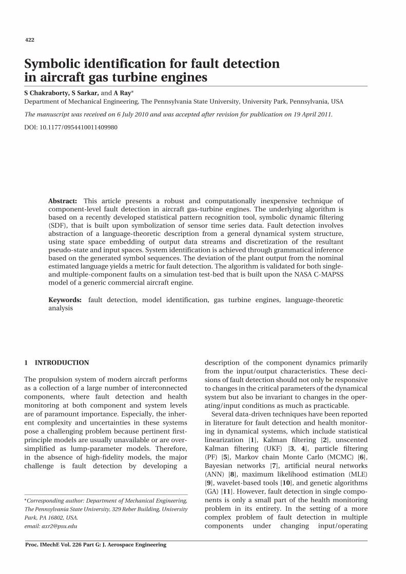
The crux of the method is to place the boundaries of
the partition segments in such a way, that a change
in both input and output symbols is synchronized.
The phase space and input variables hold the last
symbol till there is a change in the output state
sequence. Periodicity (or at least quasi-periodicity)
guarantees that the number of phase space and
input symbols will not explode. The partitioning
scheme is illustrated in Fig. 2.
Remark
A partition constructed in this way is admissible,
but may not be maximal, since this partition is a
subpartition of the original partition proposed in
Theorem 3.1.
Let U ¼ {u(1), u(2), . . .} denote the discretized input
data sequence. Similarly let Q¼ {q(1), q(2), . . .} denote
the discretized state variable sequence. It is noted
that the state space can be multi-dimensional
depending on the embedding dimension m*. Once
the input and state spaces are both discretized,
they can be combined to form the discretized aug-
mented input space �¼ {�(1), �(2), . . .}, where each
�(i )¼ {q(i ), u(i )}.
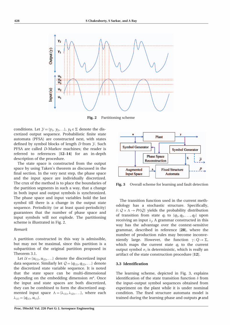
The transition function used in the current meth-
odology has a stochastic structure. Specifically,
� :Q��!Pr{Q} yields the probability distribution
of transition from state qi to {q1, q2, . . . , qf } upon
receiving an input �j. A grammar constructed in this
way has the advantage over the context-sensitive
grammar, described in reference [28], where the
number of production rules may become inconve-
niently large. However, the function g : Q!�,
which maps the current state qi to the current
output symbol �i is deterministic, which is really an
artifact of the state construction procedure [12].
3.3 Identification
The learning scheme, depicted in Fig. 3, explains
identification of the state transition function � from
the input–output symbol sequences obtained from
experiment on the plant while it is under nominal
condition. The fixed structure automata model is
trained during the learning phase and outputs p and
Fig. 2 Partitioning scheme
Fig. 3 Overall scheme for learning and fault detection
428 S Chakraborty, S Sarkar, and A Ray
Proc. IMechE Vol. 226 Part G: J. Aerospace Engineering

~p (shown using dotted arrows) are obtained during
testing (fault detection) phase and will be described
later.
It is assumed that inputs and outputs are time-
synchronized. The state transition function � can be
expanded into two dimensional matrices ��i, indexed
by the input variable alphabets. That means
� ¼ f��1 , ��2 , . . . , ��m g ð17Þ
where ��i : qj� �i!Pr{Q} maps the current state and
input to the probability distribution over all possible
states. The algorithm for estimating the matrices ��i
is straightforward and involves counting the fre-
quency of each transition in the learning phase.
Since the state transition matrices are constructed
simply by counting, this method is ideal for imple-
menting in the sensor electronics for real-time
prognoses.
The learning algorithm has to make sure that the
probability values of �i converge. The convergence
depends on the length of the input–output symbol
sequences. In this study, a stopping rule [12] has
been used for detecting the optimal data length.
In the learning phase, it has to be ensured that
the grammar G is trained with sufficient input data
belonging to a particular equivalence class. This is
the so-called coverage problem.
4 FAULT DETECTION SCHEME
The concept of fault detection is largely similar to that
of the learning phase in Fig. 3 with the following
exception. The input and output time series data
from the actual plant are discretized to form symbol
sequences, which are fed to the trained fixed struc-
ture automaton. The discretization is performed
using the same partitioning as was done during
the learning phase. It is noted that the resulting
finite state automaton (FSA) uses the output from
the actual system in addition to the input, and
hence cannot serve as an independent ‘system iden-
tification’ procedure in the classical sense of the term.
Nevertheless, the automaton can serve as a system
emulator if the state transition function � is comple-
tely deterministic. That is, given the current state qj
and the current input symbol �i
��i ðqj , �iÞ ¼ pq1pq2
. . . pqj�j
� �Tð18Þ
where pqk¼ 1 for one and only one k ð19Þ
¼ 0 otherwise ð20Þ
It can be shown that by a proper redefinition of
partitioning and depth used for the construction
of states, a stochastic automaton can be converted
to a deterministic finite state automata [29]. But
that transformation inevitably leads to state explo-
sion and uneconomical growth in the computational
complexity.
Instead, in the current scheme, the state transition
probability vectors �iqj
, which are the rows of the state
transition matrix �, serve as feature vectors, and are
used for the purpose of fault detection. An extremely
convenient feature of using state transition probabil-
ities as feature vectors, and using stochastic methods
to define distances between nominal and off-nominal
behaviours of plants is that this technique is very
robust to noise.
This article proposes a Pseudo-Learning technique
of utilizing the stochastic state transition function �
for the purpose of fault detection. In this method, the
actual state transitions inside the fixed-structure
automaton in the fault detection phase occur accord-
ing to the output symbol sequence obtained from the
actual system; and, at each instant of state transition,
the trained automaton produces a state transition
probability vector pn [29] that represents the charac-
teristics of the nominal system corresponding to
inputs at this nth instant.
It is noted that the pattern vector pn, produced by
the trained automaton, is characteristic of the nomi-
nal behaviour of the plant given the past history of
input, state, and output. The current (possibly off-
nominal) condition of the plant is characterized by
another state probability vector ~n. This is defined
for the actual system output at an instant n, for
which only one element of the vector will be 1, rest
are zeros. The next step is to use the sequences of
instantaneous state probability vectors {nn} and f ~png
obtained at each time instant, to construct a pattern
vector. Under the assumption of ergodicity of the
system, a pattern can be generated from frequency
count of the state visits over a wide time window in
case of symbolic time series analysis [12]. The equiv-
alent process in the present case would be calculation
of mean state probability vectors p and ~p from the
collections {n1, n2, . . . , nn} and f ~p1, ~p2, . . . , ~png respec-
tively over time instants 1, 2, . . . , n. During the fault
detection phase, the fixed structure automata model
(already trained), as shown in Fig. 3 is used and state
probability vectors p and ~p are obtained.
It may be noted that in an ideal case, p should con-
verge to ~p, while they should start to diverge from
each other as the fault progresses. Thus, any measure
of divergence of the two probability vectors, such
as the difference, p � ~p is a natural choice (similar
to residuals in Bayesian filtering based fault detec-
tion schemes [30]) for constructing the pattern
vector corresponding to that specific fault condition.
Once the pattern vectors for a fault condition are
Aircraft gas turbine engines 429
Proc. IMechE Vol. 226 Part G: J. Aerospace Engineering

obtained, a suitable classification algorithm, such as a
support vector machine can be utilized to create the
hyperplane separating the nominal patterns from
the possibly off-nominal pattern vectors.
Remark
In the Learning Automata literature, learning [29] is
done by continuous feedback from environment to
the automaton at each time instant. Here, also similar
feedback technique is taken but not for learning or
changing the structure or internal functions of the
finite state machine, but only to provide actual his-
tory of past outputs to the nominal automaton based
model. Hence, the technique can be called a Pseudo-
Learning Technique.
5 RESULTS AND DISCUSSION
Time series data have been collected for different sen-
sors under persistent excitation of TRA inputs that
have truncated triangular profiles. To simulate differ-
ent operating conditions, each TRA input profile has
been designed to have a wide range of mean values,
amplitude, and frequency of excitation. Specifically,
the algorithm has been tested for a mean TRA angle of
40 �, 60 �, and 80 �, with amplitude ranging from �1 �,
�2 � and �3 � and the frequency of input excitation
varying between 0.1, 0.06, and 0.04 Hz. Also, the
effects of altitude and aircraft speed have been
taken into account by collecting data, while the air-
craft is at sea-level (i.e. altitude a¼ 0.0, Mach number
M¼ 0.0) when the engine is on the ground for fault
monitoring and maintenance by the engineering per-
sonnel, as well as when it is in flight at �3000 m with
Mach number M¼ 0.3. So, the entire learning set
comprises of 3� 3� 3� 2¼ 54 operating conditions.
Figure 4 shows readings from sensor P24 at different
operating conditions for a nominal engine. Figure 5
illustrates the process of learning a PFSA from input–
output signal pairs. However, the figure shows a sim-
plified generic automata in order to explain the
underlying concept. There is no direct correspon-
dence to the actual automata used for fault detection.
Data corresponding to only 4 out of the 54 operating
conditions considered, are shown here to preserve
clarity of presentation.
The engine simulation is conducted at a frequency
of 66.67 Hz (i.e. inter-sample time of 15 ms) and
the length of the simulation time window is 150 s,
which generate 10 000 data points for each learning
or test case, out of which the last 8000 data points are
used to reduce the effects of initial transience.
An engine component C is considered to be in
nominal condition when both C and �C are equal
to 1. Fault is injected in the fan by simultaneously
reducing both C and �C by same amount in the
results reported in this article. For example,
F¼ �F¼ 0.98 signifies a 2 per cent relative loss in
efficiency and flow capacity for fan.
5.1 Detection of a single fault
To analyse a representative single component fault
situation in the current engine model, fault in fan
has been considered, which is realized by modifying
fan efficiency ( F) and flow modifier (�F). For both
learning (i.e. forward problem) and testing (i.e.
inverse problem), time series data from relevant
sensor (P24 in this case) are generated with F and
�F ranging from 1.0 to 0.96 (i.e. 4 per cent relative
loss in fan efficiency) in steps of 0.005.
The learning set comprises of the input signal pro-
file of TRA and the output signal profile of P24 for
all 54 operating conditions. The output data P24
from all these operating conditions are first normal-
ized and then concatenated to form the complete
output set. Such data are then discretized using a
maximum entropy partitioning [12]. The number of
states in the PFSA is selected to be 15. Following the
procedure outlined in section 3, the augmented input
space is constructed by discretizing the input and
phase space. In this case, the output itself suffices
as the phase space, i.e. m*¼ 1. The input specific
probabilistic state transition matrices are next con-
structed, which conclude the learning process of the
PFSA.
Fig. 4 Sensor reading at several operating conditions;in each set: solid lines imply input TRA oscilla-tion amplitude¼�1� and frequency¼ 0.1 Hz;dotted lines imply amplitude¼�2� andfrequency¼ 0.06 Hz; and dashed lines implyamplitude¼�3� and frequency¼ 0.04 Hz
430 S Chakraborty, S Sarkar, and A Ray
Proc. IMechE Vol. 226 Part G: J. Aerospace Engineering

In the validation part, the input and output data
corresponding to a single fault level (for example,
when the fan efficiency level is, say, 0.995) but for
all different input and operating conditions, are
fed into the algorithm. The pattern vector cluster cor-
responding to this fault condition is calculated
according to the algorithm described in section 3.
The success or failure of the algorithm depends on
the distinguishability of these patterns from the pat-
tern cluster generated by the machine when the
engine was running in its nominal health state,
albeit at different operating conditions.
A support vector machine (SVM) classifier with linear
kernel [31] has been used to classify the nominal from
the off-nominal cases. The validation is done by choos-
ing one of the datasets as test data and using the remain-
ing data as the learning data, and noting whether it could
be classified correctly. This is repeated for all the data-
sets to yield a true positive rate (TPR), true negative rate
(TNR), false positive rate (FPR), and false negative rate
(FNR). Here, ‘positive’ denotes nominal condition and
‘negative’ denotes off-nominality. Thus, false positive
implies a missed event, i.e. a faulty engine is classified
as healthy, and a false negative implies a false alarm, i.e.
a healthy engine is misclassified as faulty.
In order to estimate the robustness of the tech-
nique with noisy data [32, 33], the data are contam-
inated with additive white gaussian noise. The SNR
in dB is decreased from 100 dB in the first run to 10 dB
in steps of 10 dB. Figure 6 shows the output signals
contaminated with white Gaussian noise for four
different signal-to-noise intensity.
Figure 7 displays the results of the SVM classifier
when applied to patterns corresponding to different
fan efficiencies. It is noted in Fig. 7(a) that even a
decrease of 0.5 per cent in fan efficiency can be
detected with TPR¼ 100 per cent and FPR¼
0 per cent for noise contamination at SNR¼ 40 dB.
Even for SNR¼ 30 dB, the receiver operating charac-
teristic (ROC) curve [34] closely approaches the
Fig. 5 Input (TRA) and output (Pressure) signals at different operating conditions and the learntPFSA model
Aircraft gas turbine engines 431
Proc. IMechE Vol. 226 Part G: J. Aerospace Engineering

left-hand top corner. There is a significant decrease in
performance for noise contamination at SNR¼ 20 dB
and beyond.
Remark
A typical use of an ROC graph is to enable the oper-
ator to assess the risk versus the gain potential of
a decision. For example, the typical results from a
certain risk-analysis study are as follows. A 2 per cent
probability of failure to detect a degraded fan perfor-
mance is acceptable for a certain kind of aircraft
operation.
The corresponding result for a relatively larger
fault, corresponding to a decrease of 2.5 per cent in
fan efficiency, is shown in Fig. 7(b). As expected, the
noise tolerance for this classification is much higher,
since the fault signature is also less subtle. It can be
seen that an almost sure classification can be per-
formed even when SNR¼ 20 dB.
Table 2 displays the probability of actually detect-
ing failures for an allowable FPR of 2 per cent for three
different fault levels and several SNR conditions. It is
noted that for very noisy signals (SNR¼ 20 dB), subtle
faults (e.g. efficiency decrease of 0.5 per cent) are
almost impossible to detect if the probability of
missed detection is kept below 2 per cent. However,
for slightly more degraded conditions (efficiency
decrease of 3 per cent), failures can be detected with
100 per cent confidence while guaranteeing that
missed detection rate is kept below 2 per cent.
5.2 Detection of multiple faults
In an interconnected system (e.g. an gas turbine
engine), detection of multiple faults is inherently a
difficult problem, because a failure in one of the
components, say Component A essentially changes
the input conditions to some other component, say
Component B and then off-nominal performance of
Component B can either be due to an actual fault in
Component B or due to the off-nominal input received
by it. Thus, probabilities of missed detections and/or
false alarms tend to rise. To resolve this problem, the
key idea here is to treat possible fault conditions of
Component A as different operating conditions for
Component B and then to follow the similar procedure
as before. In order to test the reliability of the
algorithm against simultaneously occurring faults,
two components have been chosen. The fan is
assumed to be slowly deteriorating in terms of its
efficiency as both F and �F are decreased from
their nominal values of 1. However, in contrast
(a)
(b)
Fig. 7 ROC of symbolic identification classifier atdifferent SNRs
(a) (b) (c) (d)
Fig. 6 Effects of additive white noise on pressure sensor data: signal- to noise ratio (SNR)decreasing from left to right
432 S Chakraborty, S Sarkar, and A Ray
Proc. IMechE Vol. 226 Part G: J. Aerospace Engineering

to the last simulation study, three levels of faults are
considered here:
(a) ‘low’, where F¼ �F¼ 0.995;
(b) ‘medium’, where F¼ �F¼ 0.975;
(c) ‘high’, where F¼ �F¼ 0.960.
At the same time, further down the gas path, the
low-pressure turbine also undergoes similar types
of faults, i.e. LPT¼ �LPT¼ 0.995, 0.975, and 0.960
progressively. The low-pressure turbine has been
chosen as the second component to fail, because not
only the turbine inlet temperature and pressure are
dependent on the fan operation but also the turbine
is directly mechanically linked to the fan through a
shaft. This close interconnection obviously
makes the problem of unambiguous detection much
harder.
Similar to the last simulation study, the robustness
of the algorithm is tested by running the engine
at different operating conditions. The main actuator
input TRA is again varied to have a wide range in
mean, amplitude as well as frequency. The mean
takes on three different values, 40 �, 60 �, and 80 �,
with amplitude ranging from �1 �, �2 �, and �3 �
and the frequency of input excitation varying
between 0.1, 0.06, and 0.04 Hz. Altitude and mach
number are changed to simulate both ground opera-
tion and flight at � 3600 m. These two testing envi-
ronments combined together with 3� 3� 3¼ 27
types of throttle inputs result in 54 operating condi-
tions in all. However, the four health conditions
(nominal and three fault conditions as defined
before) of the fan appear as four new operating con-
dition for the low-pressure turbine, since faults in the
fan effectively change the input condition down-
stream. The same holds for LPT faults also. Hence,
effectively, the number of operating conditions for
which each component is tested turns out to be
54� 4¼ 216.
The simulation studies are divided into two parts:
(a) Part 1, where faults in the fan are identified in the
presence of faults in the LPT;
(b) Part 2, where faults in the LPT are identified in
the presence of faults in the fan.
The signals monitored for detection of fan faults
remain the same as those in the final section, i.e.
TRA is used as the input signal profile, while P24
as the output signal. The output signal is discretized
into 15 states with maximum entropy partitioning.
The procedure explained in section 3 is followed
exactly, and the results obtained are displayed in
the left-hand side of Fig. 8.
Temperature sensors at the input and output of the
low-pressure turbine, T48 and T 50, respectively, are
simultaneously monitored for change detection in
the LPT. Although sensors to monitor T 50 are not
generally used in commercial engines, they could be
mounted easily as LPT exit typically does not present
any harsher environment compared to those at the
other usual sensor locations. A similar processing
yields the pattern vectors corresponding to each
operating conditions.
For a faulty condition of the component under
investigation, say a drop in relative efficiency of
0.005, the pattern vectors generated for all 216 oper-
ating conditions are tested for their ‘classifiability’
from pattern vectors generated by the healthy com-
ponent for the same 216 operating conditions.
The top row in Fig. 8 shows the receiver-operating
characteristics, i.e. the rate of correct and false diag-
noses when the components have failed to a very
small degree. Figures 8(a) and (b) shows that the algo-
rithm becomes less and less trustworthy as the noise
level increases for ‘low’ level faults. Compared to the
last simulation study with single faults, where even at
SNR¼ 40 dB, 100 per cent correct classification was
possible, this simulation is conducted in the presence
of faults in other components having several trade-
offs between TPR and FPR. As the fault signatures
become stronger, almost certain detection of faults
is possible even in the presence of substantial noise
(i.e. SNR¼ 40 dB). This is illustrated for ‘medium’
level faults (i.e. efficiency¼ 0.975) in both fan and
LPT in Figs 8(c) and (d), respectively. For ‘high’ level
faults (i.e. efficiency¼ 0.960), the same trend is visible
in Figs 8(e) and (f). Similar to Table 2 for single-com-
ponent faults, Table 3 provides the probability of
actually detecting failures for an allowable FPR of
2 per cent for three different fault levels and several
SNR conditions.
Table 2 Fault detection rates for an allowable false positive rate of 2 per cent for different fault
levels and several SNR conditions
Fan efficiencies
SNR 0.995% 0.990% 0.985% 0.980% 0.975% 0.970% 0.965% 0.960%
20 9.26% 35.19% 66.67% 88.89% 98.15% 100.00% 100.00% 100.00%30 70.37% 100.00% 100.00% 100.00% 100.00% 100.00% 100.00% 100.00%40 100.00% 100.00% 100.00% 100.00% 100.00% 100.00% 100.00% 100.00%
Aircraft gas turbine engines 433
Proc. IMechE Vol. 226 Part G: J. Aerospace Engineering
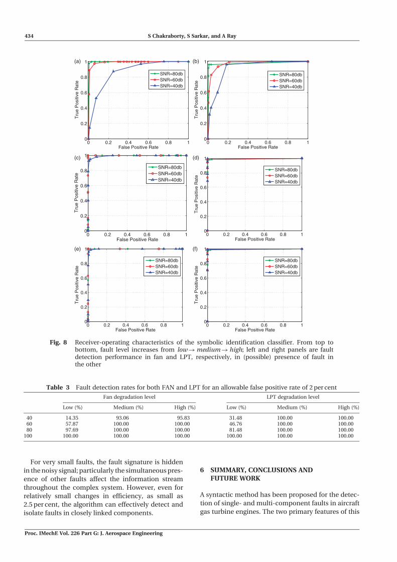
For very small faults, the fault signature is hidden
in the noisy signal; particularly the simultaneous pres-
ence of other faults affect the information stream
throughout the complex system. However, even for
relatively small changes in efficiency, as small as
2.5 per cent, the algorithm can effectively detect and
isolate faults in closely linked components.
6 SUMMARY, CONCLUSIONS ANDFUTURE WORK
A syntactic method has been proposed for the detec-
tion of single- and multi-component faults in aircraft
gas turbine engines. The two primary features of this
0 0.2 0.4 0.6 0.8 10
0.2
0.4
0.6
0.8
1
False Positive Rate
Tru
e P
ositi
ve R
ate
SNR=80dbSNR=60dbSNR=40db
0 0.2 0.4 0.6 0.8 10
0.2
0.4
0.6
0.8
1
False Positive Rate
Tru
e P
ositi
ve R
ate
SNR=80dbSNR=60dbSNR=40db
0 0.2 0.4 0.6 0.8 10
0.2
0.4
0.6
0.8
1
False Positive Rate
Tru
e P
ositi
ve R
ate
SNR=80dbSNR=60dbSNR=40db
0 0.2 0.4 0.6 0.8 10
0.2
0.4
0.6
0.8
1
False Positive Rate
Tru
e P
ositi
ve R
ate
SNR=80dbSNR=60dbSNR=40db
0 0.2 0.4 0.6 0.8 10
0.2
0.4
0.6
0.8
1
False Positive Rate
Tru
e P
ositi
ve R
ate
SNR=80dbSNR=60dbSNR=40db
0 0.2 0.4 0.6 0.8 10
0.2
0.4
0.6
0.8
1
False Positive Rate
Tru
e P
ositi
ve R
ate
SNR=80dbSNR=60dbSNR=40db
(a) (b)
(c) (d)
(e) (f)
Fig. 8 Receiver-operating characteristics of the symbolic identification classifier. From top tobottom, fault level increases from low!medium!high; left and right panels are faultdetection performance in fan and LPT, respectively, in (possible) presence of fault inthe other
Table 3 Fault detection rates for both FAN and LPT for an allowable false positive rate of 2 per cent
Fan degradation level LPT degradation level
Low (%) Medium (%) High (%) Low (%) Medium (%) High (%)
40 14.35 93.06 95.83 31.48 100.00 100.0060 57.87 100.00 100.00 46.76 100.00 100.0080 97.69 100.00 100.00 81.48 100.00 100.00
100 100.00 100.00 100.00 100.00 100.00 100.00
434 S Chakraborty, S Sarkar, and A Ray
Proc. IMechE Vol. 226 Part G: J. Aerospace Engineering
fault detection method are: (a) symbolic identification
and (b) pseudo-learning. A PFSA model of the process
dynamics is constructed from the input–output data;
the PFSA representation is analogous to a non-linear
system model that is functionally equivalent to a
linear system transfer function. The reported work
is a step towards building a real-time data-driven
tool for estimation of parametric conditions in com-
plex dynamical systems. Scalability may become a
critical issue for this method of fault detection with
increase in number of components and fault levels.
However, a natural way to circumvent this problem is
to perform isolation of a faulty subsystem with a rel-
atively small number of components before detection
of a fault in a particular component [14, 15].
Further theoretical, computational, and experi-
mental work is necessary before this fault detection
tool can be considered for incorporation into the
instrumentation and control system of aircraft
engines. For example, real flight record data and envi-
ronmental condition data need to be incorporated to
investigate the effects of atmospheric temperature
and pressure variations on the fault detection algo-
rithm. The following theoretical topics are currently
under investigation:
(a) development of a multi-dimensional partitioning
for a MIMO system, which should be computa-
tionally inexpensive;
(b) development of a comprehensive sensor fusion
algorithm to handle multiple sensor data simulta-
neously for detection;
(c) estimation of a theoretical bound on the error
incurred in this process of fault detection;
(d) extension of the symbolic identification tech-
nique to incorporate transient engine operations,
i.e. during take-off, climb, or landing;
(e) generation of the health status at the vehicle level
via linguistic methods [35].
FUNDING
This work has been supported in part by NASA under
Cooperative Agreement No. NNX07AK49A, and by the
U.S. Army Research Laboratory and Army Research
Office under Grant No. W911NF-07-1-0376. Any opi-
nions, findings and conclusions or recommendations
expressed in this publication are those of the authors
and do not necessarily reflect the views of the
Sponsoring agencies.
� Pennsylvania State University, University Park, PA
16802, USA 2011
REFERENCES
1 Broersen, P. Estimation of parameters of non-lineardynamical systems. Int. J. Non-linear Mech., 1974, 9,355–361.
2 Van Lith, P., Witteveen, H., Betlem, B., and Roffel,B. Multiple nonlinear parameter estimation usingpi feedback control. Control Eng. Pract., 2001, 9,517–531.
3 Wan, E. and Van der Merwe, R. The unscentedkalman filter for nonlinear estimation. InProceedings of the IEEE Symposium 2000 ASSPCC,Lake Louise, Alta, Canada, 1–4 October 2000,pp. 153–158.
4 Julier, S. and Uhlmann, J. A new extension of thekalman filter to nonlinear systems. Proc. SPIE,1997, 3068, 182–193.
5 Ching, J., Beck, J., and PorterChin, K. Bayesianstate and parameter estimation of uncertaindynamical systems. Prob. Eng. Mech., 2006, 21(1),81–96.
6 Bremer, C. and Kaplan, D. Markov chain MonteCarlo estimation of nonlinear dynamics from timeseries. Physica D, 2001, 160, 116–126.
7 Wang, Y. and Geng, L. Bayesian network basedfault section estimation in power systems. In IEEERegion 10 Annual International Conference,TENCON, Hong Kong, China, 14–17 November 2006.
8 Hoffman, A. and van der Merwe, N. The applicationof neural networks to vibrational diagnostics formultiple fault conditions. Comput. Stand.Interfaces, 2002, 24(2), 139–149.
9 David, B. and Bastin, G. Parameter estimation innonlinear systems with auto and crosscorrelatednoise. Automatica, 2002, 38, 81–90.
10 Ghanem, R. and Romeo, F. A wavelet-basedapproach for model and parameter identification ofnon-linear systems. Int. J. Non-linear Mech., 2001,36, 835–859.
11 Yao, L. and Sethares, W. Nonlinear parameter esti-mation via the genetic algorithm. IEEE Trans. SignalProcess., 1994, 42(4), 927–935.
12 Ray, A. Symbolic dynamic analysis of complex sys-tems for anomaly detection. Signal Process., 2004,84(7), 1115–1130.
13 Rajagopalan, V. and Ray, A. Symbolic time seriesanalysis via waveletbased partitioning. SignalProcess., 2006, 86(11), 3309–3320.
14 Gupta, S., Ray, A., Sarkar, S., and Yasar, M. Faultdetection and isolation in aircraft gas turbineengines. Part 1: Underlying concept. Proc.IMechE, Part G: J. Aerospace Engineering, 2008,222(3), 307–318.
15 Sarkar, S., Yasar, M., Gupta, S., Ray, A., andMukherjee, K. Fault detection and isolation inaircraft gas turbine engines. Part 2: Validation on asimulationtest bed. Proc. IMechE, Part G: J. AerospaceEngineering, 2008, 222(3), 319–330.
16 Sarkar, S., Rao, C., and Ray, A. Statistical estimationof multiple faults in aircraft gas turbine engines.Proc I MechE Part G: J. Aerospace Engineering, 2009,223(4), 415–424.
Aircraft gas turbine engines 435
Proc. IMechE Vol. 226 Part G: J. Aerospace Engineering
17 Rao, C., Ray, A., Sarkar, S., and Yasar, M. Reviewand comparative evaluation of symbolic dynamic fil-tering for detection of anomaly patterns, 2008. DOI10.1007/s11760-008-0061-8.
18 Subbu, A. and Ray, A. Space partitioning via Hilberttransform for symbolic time series analysis. Appl.Phys. Lett., 2008, 92(08), 084107.
19 Frederick, D., DeCastro, J., and Litt, J. Users guidefor the commercial modular aero-propulsion systemsimulation (c-mapss), October 2007, NASA/TM2007-215026.
20 C-MAPSS: Commercial modular aero-propulsionsystem simulation, NASA GRC Software Repository,2007.
21 Kobayashi, T. and Simon, D. A hybrid neural net-work-genetic algorithm technique for aircraft engineperformance diagnostics. In Proceedings of the 37thJoint Propulsion Conference and Exhibit co-spon-sored by the AIAA, ASME, SAE, and ASEE, Salt LakeCity, Utah, 8–11 July 2001.
22 Hopcroft, J., Motwani, R., and Ullman, J.Introduction to automata theory, languages, andcomputation, 3rd edition, 2006 (Addison-WesleyLongman Publishing Co., Inc., Boston,Massachusetts, USA).
23 Kokar, M. On consistent symbolic representationsof general dynamic systems. IEEE Trans. Syst. ManCybernetics, 1995, 25(8), 1231–1242.
24 Levy, L. Discrete structures of computer science, 1980(John Wiley & Sons, New York).
25 Takens, F. Detecting strange attractors in turbu-lence, Vol. 898/1981, 1981 (Springer, Berlin/Heidelberg).
26 Gautama, T., Mandic, D., and Hulle, M. V. A dif-ferential entropy based method for determining
the optimal embedding parameters of a signal.In Proceedings of the IEEE InternationalConference on Acoustics, speech, and signal pro-cessing, Hong Kong, China, Vol. 6 (6–10) pp. VI-29-32, 6–10 April 2003.
27 Beirlant, J., Dudewicz, E. J., Gyrfi, L., and Meulen,E. C. Nonparametric entropy estimation: An over-view. Int. J. Math. Stat. Sci., 1997, 6, 17–39.
28 Martins, J., Dente, J., Pires, A., and Mendes, R.Language identification of controlled systems:Modeling, control, and anomaly detection. IEEETrans. Syst. Man Cybernetics, Part C: ApplicationsAnd Reviews 2007, May.
29 Narendra, K. and Thathachar, M. Learning autom-ata an introduction, 1989 (Prentice-Hall, UpperSaddle River, New Jersey, USA).
30 Kobayashi, T. and Simon, D. L. Hybrid kalman fil-ter approach for aircraft engine in-flight diagnostics:Sensor fault detection case. J. Eng. Gas TurbinesPower, 2007, 129, 746–754.
31 Duda, R., Hart, P., and Stork, D. Pattern classifica-tion, 2001 (John Wiley & Sons Inc., New York).
32 Simon, D. L. and Garg, S. Optimal tuner selectionfor kalman filterbased aircraft engine performanceestimation. J. Eng. Gas Turbines Power, 2010,132(3), 031601.
33 Lu, P., Zhang, M., Hsu, T., and Zhang, J. An evalu-ation of engine faults diagnostics using artificialneural networks. J. Eng. Gas Turbines Power, 2001,123(2), 340–346.
34 Poor, V. An introduction to signal detection andestimation, 2nd edition, 1988 (Springer-Verlag,New York, USA).
35 Yang, T. Computational verb theory: Ten years later.Int. J. Comput. Cognit., 2007, 5, 63–86.
436 S Chakraborty, S Sarkar, and A Ray
Proc. IMechE Vol. 226 Part G: J. Aerospace Engineering