symbolic computation of local symmetries of nonlinear and

Symbolic Computation of Local Symmetries of Nonlinear and

Linear Partial and Ordinary Differential Equations

Alexei F. Cheviakova),Department of Mathematics and Statistics, University of Saskatchewan, Saskatoon, S7N 5E6 Canada

September 19, 2011

Abstract

The paper illustrates the use of a symbolic software package GeM for Maple to compute lo-cal symmetries of nonlinear and linear differential equations (DE). In the cases when a givenDE system contains arbitrary functions or parameters, symbolic symmetry classification is per-formed.

Special attention is devoted to the computation of point symmetries of linear PDE systems.Routines are available that effectively eliminate infinite obvious symmetries of linear differentialequations.

1 Introduction

A symmetry of a system of ordinary or partial differential equations (ODE, PDE) is any trans-formation of its solution manifold into itself, i.e., a symmetry maps any solution of a DE systemto another solution of the same system. Continuous symmetries of DE systems are hence definedtopologically, and in principle, any nontrivial DE system has symmetries. The practical problemconsists in finding algorithmic ways of computation of such symmetries. In the latter part of the19th century, Sophus Lie showed that the problem of finding the Lie group of point transformations(point symmetries) leaving invariant an equation (algebraic, or ODE, or PDE), reduced to solvingrelated linear systems of determining equations for components of its infinitesimal generators. Lie’salgorithm for finding point symmetries of a DE system can be extended to find more general localsymmetries admitted by DEs, where one allows the symmetry components to depend on derivativesof dependent variables.

The structure of local symmetry groups admitted by different ODE and PDE systems containsessential information about the given DE system, and thus can vary greatly. For example, everyfirst-order scalar ODE has an infinite-parameter Lie group of point symmetries. A second-orderscalar ODE has at most an eight-parameter Lie group of point symmetries; a scalar ODE of ordern ≥ 3 has at most n + 4 independent point symmetries (see [1], Section 3.7). PDEs and PDEsystems can have finite- or infinite-parameter Lie groups of point transformations. In particular,linear PDE systems and PDE systems that can be mapped into linear PDE systems through aninvertible transformation admit infinite-parameter Lie groups of point symmetries.

Symmetries of ordinary differential equations are used for reduction of order and complete in-tegration, as well as for the construction of invariant solutions ( [1], Chapter 3). Symmetries ofpartial differential equations yield reductions of order and/or number of variables. Invariant (inparticular, self-similar) solutions that arise from reduced systems often have transparent physicalmeaning. Many appropriate examples are found in [2]. Infinite-dimensional symmetry groups are

a)Corresponding author. Electronic mail: [email protected]

1

used for the construction of families of new exact solutions from known ones (e.g. [3]). For a non-linear PDE system, from its admitted symmetry group, one can determine whether or not it canbe mapped into a linear system by an invertible transformation, and find the explicit form of thattransformation ( [4], Chapter 2).

Many extensions of the notion of local symmetries are known, including nonlocal symmetries,approximate symmetries, the nonclassical method, etc. For a detailed review, the reader is referredto [2, 4, 5] and references therein.

Application of Lie’s symmetry method and its extensions to nontrivial DE systems often requiresextensive algebraic manipulation. For many contemporary DE models, especially those that dopossess non-trivial symmetry structure, such analysis presents a significant computational challenge.In particular, symmetry determining equations split into overdetermined systems of linear PDEsfor the unknown symmetry components; such linear overdetermined systems can commonly containhundreds or thousands of determining equations. To treat such huge systems, symbolic computersoftware is normally used.

A symbolic package for computations of symmetries naturally consists of two parts. The first partcontains user routines that interpret equations, use a specified ansatz for symmetry componentsor conservation law multipliers, generate determining equations, and split them into an overdeter-mined linear PDE system. The second part contains routines for effective symbolic reduction andsolution of large overdetermined PDE systems. Since DE systems often involve arbitrary consti-tutive functions and/or parameters, it is highly beneficial when the reduction algorithm allows forcase splitting, i.e., the isolation of special forms of constitutive functions and/or parameters, forwhich additional symmetries arise.

Several methods for reduction of large overdetermined systems of partial differential equationshave been developed (for review, see e.g. [8–11].) Many of these methods have been implemented invarious symbolic software packages. In particular, the excellent rif package of Maple based on thework in [17–19] is one of the core components of Maple’s symbolic differential equations toolbox.

To date, a number of packages for the computation of symmetries has been developed for differentcomputer algebra systems (CAS). For example, one can name a set of programs LiePDE, ApplySym[6] that provide a user interface for local symmetry computation in CAS REDUCE; a set of programsfor symmetry computations in Mathematica is described in [7]. For reviews of symbolic softwarefor symmetry analysis and related problems, the reader is referred to [8–11] and [4], Chapter 5.

The package GeM for Maple described in this work offers a set of simple and general routines thatgenerate and split the systems of determining equations for the computations of local conserva-tion laws, symmetries and approximate symmetries for wide classes of differential equations andDE systems. It subsequently uses rif for case splitting and solution of overdetermined systems,and contains additional of routines for the symmetry output, as well as other important routinesdescribed in this paper.

The current paper explains and illustrates the use of the latest version of GeM package to performsymbolic computations of local symmetries of linear and nonlinear differential equations.

In Section 2, the notation and general algorithms for local symmetry analysis are briefly re-viewed. A special computational difficulty is presented by systems of linear PDEs, since theyadmit an infinite set of obvious point symmetries, corresponding to addition of arbitrary solutionsof the corresponding linear homogeneous system. In Section 2.3, theorems and a general conjecturepertaining to point symmetries of linear equations are presented and discussed.

In Section 3, the principal sequence of symmetry analysis using GeM package for Maple is reviewed,and some features of the package structure and its routines are highlighted.

Section 4 contains run examples for point symmetry analysis of a third-order nonlinear ODE andhigher-order symmetry computations for the Korteweg-de Vries equation [25].

2

To study symmetries of DE systems involving arbitrary function(s) and/or constant parameter(s),a symmetry classification must be performed. Section 5 discusses this problem, the related problemof finding and using equivalence transformations, and their symbolic implementations. As anexample, equivalence transformations are computed and point symmetries are classified for a familyof a nonlinear diffusion equations.

Section 6 contains an example of symmetry analysis of a linear PDE system. The example employsGeM package routines which use a special ansatz discussed in Section 2.3, in order to automaticallyexclude obvious infinite symmetries of linear equations.

Section 7 concludes the paper with some discussion.

2 Local symmetries of differential equations

Consider a system of N differential equations of order k, with n independent variables x =(x1, . . . , xn) and m dependent variables u(x) = (u1(x), . . . , um(x)), given by

Rσ(x, u, ∂u, . . . , ∂ku) = 0, σ = 1, . . . , N. (2.1)

[For ODE systems, N = 1.] The notation

∂u ≡ ∂1u =(u1

1(x), . . . , u1n(x), . . . , um

1 (x), . . . , umn (x)

)

denotes the set of all first-order partial derivatives;

∂pu ={

uµi1...ip

| µ = 1, . . . , m; i1, . . . , ip = 1, . . . , n}

={

∂puµ(x)∂xi1 . . . ∂xip

| µ = 1, . . . , m; i1, . . . , ip = 1, . . . , n

}

denote higher-order derivatives.Summation in any pair of repeated indices is assumed throughout the paper.

2.1 Point symmetries

Consider a one-parameter Lie group of point transformations

(x∗)i = f i(x, u; ε) = xi + εξi(x, u) + O(ε2), i = 1, . . . , n,(u∗)µ = gµ(x, u; ε) = uµ + εηµ(x, u) + O(ε2), µ = 1, . . . ,m,

(2.2)

with the corresponding infinitesimal generator

X = ξi(x, u)∂

∂xi+ ηµ(x, u)

∂

∂uµ. (2.3)

The kth extension (prolongation) of (2.3) is given by

X(k) = ξi(x, u)∂

∂xi+ ηµ(x, u)

∂

∂uµ+ η

(1) µi (x, u, ∂u)

∂

∂uµi

+ . . . + η(k) µi1...ik

(x, u, ∂u, . . . , ∂ku)∂

∂uµi1...ik

,(2.4)

where the prolonged components η(1) µi , . . ., η

(k) µi1...ik

are defined in terms of {ξi(x, u), ηµ(x, u)} by

η(1) µi = Diη

µ − (Diξj)uµ

j , (2.5)

3

and

η(k) µi1...ik

= Dikη(k−1) µi1...ik−1

− (Dikξj)uµi1...ik−1j , (2.6)

for µ = 1, . . . , m, and i, ij = 1, . . . , n for j = 1, . . . , k, and

Di =∂

∂xi+ uµ

i

∂

∂uµ+ uµ

ii1

∂

∂uµi1

+ uµii1i2

∂

∂uµi1i2

+ · · · , (2.7)

i = 1, . . . , n.

Definition 2.1. A one-parameter Lie group of point transformations (2.2) leaves the DE system(2.1) invariant if and only if its kth extension (2.4) leaves invariant the solution manifold of (2.1)in (x, u, ∂u, . . . , ∂ku)-space, i.e., it maps any family of solution surfaces u = u(x) of the DE system(2.1) into another family of solution surfaces u∗ = u∗(x∗) of DE system (2.1). In this case, theone-parameter Lie group of point transformations (2.2) is called a point symmetry of the DE system(2.1).

Lie’s algorithm to find the point symmetries of a given DE system (2.1) is given by the followingtheorem.

Theorem 2.1. Let (2.3) be the infinitesimal generator of a one-parameter Lie group of pointtransformations (2.2). Let (2.4) be its kth extension. Then the transformation (2.2) is a pointsymmetry of the DE system (2.1) if and only if for each α = 1, . . . , N ,

X(k)Rα(x, u, ∂u, . . . , ∂ku) = 0, (2.8)

when

Rσ(x, u, ∂u, . . . , ∂ku) = 0, σ = 1, . . . , N. (2.9)

The proof appears in [12], with the restriction that the given system (2.1) can be written in asolved form in terms of a set of leading derivatives.

In order to find point symmetries admitted by a given DE system (2.1), one needs to determine theunknown symmetry components ξi, ηµ that appear in the symmetry generator (2.3). The algorithmproceeds in the following steps.

1. Obtain determining equations by substituting the given DEs (2.9) (as well as, possibly, dif-ferential consequences of (2.9)) into the invariance condition (2.8) (in order to restrict to thesolution manifold).

2. Obtain the split system of determining equations, using the fact that ξi, ηµ do not dependon derivatives of u, i.e., setting coefficients at all independent combinations of derivatives ofdependent variables in determining equations to zero.

In practice, split systems of determining equations can be rather large. For example, for thesystem of adiabatic compressible plasma equilibrium equations, one obtains 188 linear PDEs for 13unknown functions [13]. Split systems containing over a thousand determining equations are alsonot uncommon.

4

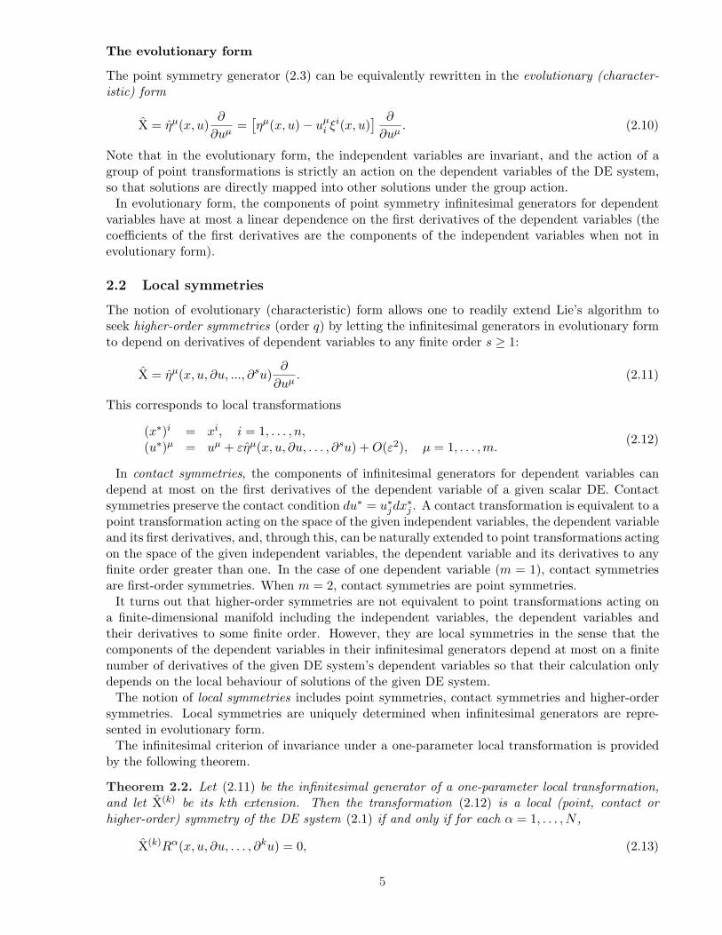
The evolutionary form

The point symmetry generator (2.3) can be equivalently rewritten in the evolutionary (character-istic) form

X = ηµ(x, u)∂

∂uµ=

[ηµ(x, u)− uµ

i ξi(x, u)] ∂

∂uµ. (2.10)

Note that in the evolutionary form, the independent variables are invariant, and the action of agroup of point transformations is strictly an action on the dependent variables of the DE system,so that solutions are directly mapped into other solutions under the group action.

In evolutionary form, the components of point symmetry infinitesimal generators for dependentvariables have at most a linear dependence on the first derivatives of the dependent variables (thecoefficients of the first derivatives are the components of the independent variables when not inevolutionary form).

2.2 Local symmetries

The notion of evolutionary (characteristic) form allows one to readily extend Lie’s algorithm toseek higher-order symmetries (order q) by letting the infinitesimal generators in evolutionary formto depend on derivatives of dependent variables to any finite order s ≥ 1:

X = ηµ(x, u, ∂u, ..., ∂su)∂

∂uµ. (2.11)

This corresponds to local transformations

(x∗)i = xi, i = 1, . . . , n,(u∗)µ = uµ + εηµ(x, u, ∂u, . . . , ∂su) + O(ε2), µ = 1, . . . ,m.

(2.12)

In contact symmetries, the components of infinitesimal generators for dependent variables candepend at most on the first derivatives of the dependent variable of a given scalar DE. Contactsymmetries preserve the contact condition du∗ = u∗jdx∗j . A contact transformation is equivalent to apoint transformation acting on the space of the given independent variables, the dependent variableand its first derivatives, and, through this, can be naturally extended to point transformations actingon the space of the given independent variables, the dependent variable and its derivatives to anyfinite order greater than one. In the case of one dependent variable (m = 1), contact symmetriesare first-order symmetries. When m = 2, contact symmetries are point symmetries.

It turns out that higher-order symmetries are not equivalent to point transformations acting ona finite-dimensional manifold including the independent variables, the dependent variables andtheir derivatives to some finite order. However, they are local symmetries in the sense that thecomponents of the dependent variables in their infinitesimal generators depend at most on a finitenumber of derivatives of the given DE system’s dependent variables so that their calculation onlydepends on the local behaviour of solutions of the given DE system.

The notion of local symmetries includes point symmetries, contact symmetries and higher-ordersymmetries. Local symmetries are uniquely determined when infinitesimal generators are repre-sented in evolutionary form.

The infinitesimal criterion of invariance under a one-parameter local transformation is providedby the following theorem.

Theorem 2.2. Let (2.11) be the infinitesimal generator of a one-parameter local transformation,and let X(k) be its kth extension. Then the transformation (2.12) is a local (point, contact orhigher-order) symmetry of the DE system (2.1) if and only if for each α = 1, . . . , N ,

X(k)Rα(x, u, ∂u, . . . , ∂ku) = 0, (2.13)

5

when

Rσ(x, u, ∂u, . . . , ∂ku) = 0, σ = 1, . . . , N,

∂lRσ(x, u, ∂u, . . . , ∂ku) = 0, l = 1, . . . , s, σ = 1, . . . , N. (2.14)

[Note that if a particular DE Rσ(x, u, ∂u, . . . , ∂k′u) = 0 has order k′ < k, then all its differentialconsequences ∂lRσ(x, u, ∂u, . . . , ∂k′u) = 0, l = 1, . . . , s + k − k′, must be computed and used insubstitutions.]

The local symmetry analysis algorithm therefore consists in determining the symmetry compo-nents ηµ(x, u, ∂u, ..., ∂su), and involves the following steps.

1. Obtain determining equations by substituting the given DEs (2.14) and their differentialconsequences into the invariance condition (2.13) (in order to restrict to the solution manifold).

2. Obtain the split system of determining equations, using the fact that ηµ only depend on deriva-tives of order up to s, i.e., setting coefficients at all independent combinations of derivativesof dependent variables of order greater than s to zero in determining equations.

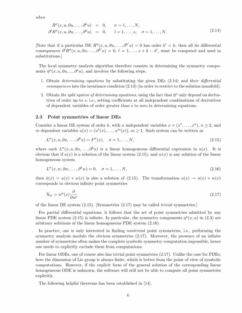
2.3 Point symmetries of linear DEs

Consider a linear DE system of order k, with n independent variables x = (x1, . . . , xn), n ≥ 2, andm dependent variables u(x) = (u1(x), . . . , um(x)), m ≥ 1. Such system can be written as

Lσ(x, u, ∂u, . . . , ∂ku) = F σ(x), σ = 1, . . . , N, (2.15)

where each Lσ(x, u, ∂u, . . . , ∂ku) is a linear homogeneous differential expression in u(x). It isobvious that if u(x) is a solution of the linear system (2.15), and w(x) is any solution of the linearhomogeneous system

Lσ(x, w, ∂w, . . . , ∂kw) = 0, σ = 1, . . . , N, (2.16)

then u(x) = u(x) + w(x) is also a solution of (2.15). The transformation u(x) → u(x) + w(x)corresponds to obvious infinite point symmetries

Xtr = wµ(x)∂

∂uµ(2.17)

of the linear DE system (2.15). [Symmetries (2.17) may be called trivial symmetries.]

For partial differential equations, it follows that the set of point symmetries admitted by anylinear PDE system (2.15) is infinite. In particular, the symmetry components ηµ(x, u) in (2.3) arearbitrary solutions of the linear homogeneous PDE system (2.16).

In practice, one is only interested in finding nontrivial point symmetries, i.e., performing thesymmetry analysis modulo the obvious symmetries (2.17). Moreover, the presence of an infinitenumber of symmetries often makes the complete symbolic symmetry computation impossible, henceone needs to explicitly exclude them from computations.

For linear ODEs, one of course also has trivial point symmetries (2.17). Unlike the case for PDEs,here the dimension of Lie group is always finite, which is better from the point of view of symboliccomputations. However, if the explicit form of the general solution of the corresponding linearhomogeneous ODE is unknown, the software will still not be able to compute all point symmetriesexplicitly.

The following helpful theorems has been established in [14].

6

Theorem 2.3. Suppose (2.15) is a scalar linear PDE (i.e., N = m = 1, n ≥ 2) of order k ≥ 2.Then components ξi, η of all of its point transformations (2.2) satisfy

∂ξi

∂u=

∂2η

∂u2= 0, i = 1, . . . , n. (2.18)

Theorem 2.4. Suppose (2.15) is a scalar linear ODE (i.e., N = m = n = 1) of order k ≥ 3. Thencomponents ξ, η of all of its point transformations (2.2) satisfy

∂ξ

∂u=

∂2η

∂u2= 0. (2.19)

Ovsiannikov ( [15], Chapter 6) states that the above result, i.e., independence of ξ’s on the depen-dent variables, and linear dependence of η’s on the dependent variables, holds for the “majority oflinear DEs” (that is, PDE and ODE systems). In general, this “linear DE conjecture” is formulatedas follows.

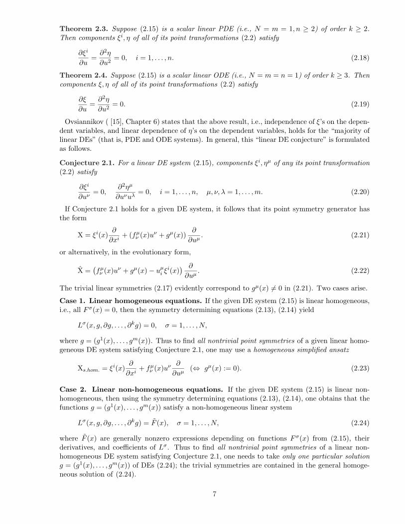
Conjecture 2.1. For a linear DE system (2.15), components ξi, ηµ of any its point transformation(2.2) satisfy

∂ξi

∂uν= 0,

∂2ηµ

∂uνuλ= 0, i = 1, . . . , n, µ, ν, λ = 1, . . . ,m. (2.20)

If Conjecture 2.1 holds for a given DE system, it follows that its point symmetry generator hasthe form

X = ξi(x)∂

∂xi+ (fµ

ν (x)uν + gµ(x))∂

∂uµ. (2.21)

or alternatively, in the evolutionary form,

X =(fµ

ν (x)uν + gµ(x)− uµi ξi(x)

) ∂

∂uµ. (2.22)

The trivial linear symmetries (2.17) evidently correspond to gµ(x) 6= 0 in (2.21). Two cases arise.

Case 1. Linear homogeneous equations. If the given DE system (2.15) is linear homogeneous,i.e., all F σ(x) = 0, then the symmetry determining equations (2.13), (2.14) yield

Lσ(x, g, ∂g, . . . , ∂kg) = 0, σ = 1, . . . , N,

where g = (g1(x), . . . , gm(x)). Thus to find all nontrivial point symmetries of a given linear homo-geneous DE system satisfying Conjecture 2.1, one may use a homogeneous simplified ansatz

Xs.hom. = ξi(x)∂

∂xi+ fµ

ν (x)uν ∂

∂uµ(⇔ gµ(x) := 0). (2.23)

Case 2. Linear non-homogeneous equations. If the given DE system (2.15) is linear non-homogeneous, then using the symmetry determining equations (2.13), (2.14), one obtains that thefunctions g = (g1(x), . . . , gm(x)) satisfy a non-homogeneous linear system

Lσ(x, g, ∂g, . . . , ∂kg) = F (x), σ = 1, . . . , N, (2.24)

where F (x) are generally nonzero expressions depending on functions F σ(x) from (2.15), theirderivatives, and coefficients of Lσ. Thus to find all nontrivial point symmetries of a linear non-homogeneous DE system satisfying Conjecture 2.1, one needs to take only one particular solutiong = (g1(x), . . . , gm(x)) of DEs (2.24); the trivial symmetries are contained in the general homoge-neous solution of (2.24).

7

Remark 2.1. (When does Conjecture 2.1 hold?) In general, conditions on linear DE systemsthat satisfy Conjecture 2.1 are unknown. The experience of the author confirms that the Conjectureholds for almost all linear DE systems he examined. The Conjecture generally does not holdfor scalar second-order linear ODEs. For linear PDEs, a simple counterexample is provided bythe following PDE system. Consider the linear constant-coefficient wave equation utt = uxx foru = u(x, t). The simplest of its potential systems is given by

vt = ux, vx = ut. (2.25)

One can show that the linear PDE system (2.25) has a point symmetry

Z = (u2 + v2)∂

∂u+ 2uv

∂

∂v, (2.26)

which contradicts the Conjecture 2.1. [The symmetry (2.26) is a nonlocal (potential) symmetry ofthe PDE utt = uxx.]

Remark 2.2. (Nontrivial infinite symmetries.) It is well-known that linear DE systems canhave an infinite number of point symmetries, even modulo the trivial symmetries (2.17). Thishappens when a set of functions {ξi(x), fµ

ν (x)} involves arbitrary functions. In particular, all linearPDE systems with constant coefficients have this property. Moreover, if there exists an invertibletransformation mapping a given variable coefficient linear PDE system to a constant coefficientlinear PDE system, then the given linear PDE system has an infinite number of nontrivial pointsymmetries ( [1], Section 6.5).

3 Local symmetry analysis using “GeM” package

A Maple – based package GeM has been recently developed by the author. The package routinesare capable of finding local (point, contact and higher-order) symmetries, adjoint symmetries andconservation laws of any ODE/PDE system without significant limitations on orders of derivativesand numbers of variables.

The GeM package employs an efficient representation of the system under consideration and result-ing determining equations: all dependent variables and derivatives are treated as Maple symbols,rather than functions or expressions: ∂B1/∂x ≡ B1x, etc. For example, the resulting Maple expres-sion for the divergence of a 3-vector B(x, y, z) = (B1(x, y, z), B2(x, y, z), B3(x, y, z)) becomes

∂

∂xB1(x, y, z) +

∂

∂yB2(x, y, z) +

∂

∂zB3(x, y, z) = B1x + B2y + B3z. (3.1)

This significantly speeds up the computation involving establishing, splitting and solution of sym-metry and conservation law determining equations. The final overdetermined linear PDE systemsare reduced using Maple rifsimp [19] routine.

The reduction of overdetermined systems of linear determining equations is usually the mostresource-demanding task, in particular, in problems that involve classification. Reduced systems ofdetermining equations are normally much simpler and can be subsequently integrated automatically(Maple pdsolve, dsolve) or even by hand.

After the determining equations are solved, a GeM routine is called that outputs all symmetrygenerators, thus completing the symmetry analysis.

The program sequence for local symmetry analysis includes the following steps.

1. Declaration of variables and the given DE system.

2. Construction of a set of split symmetry determining equations.

8

3. Simplification and reduction of the overdetermined set of determining equations.

4. Solution of the simplified set of determining equations.

5. Output of symmetry generators.

If the given DE system contains constitutive function(s) and/or constant parameter(s), a classifi-cation and case splitting need to be performed (see Section 5 below).

For linear DE systems, where one is only interested in finding nontrivial point symmetries, instep 4, special GeM routine can be called that verifies whether Conjecture 2.1 holds. Then onesubsequently uses the symmetry form (2.21) (and moreover, for homogeneous linear systems, thesimplified ansatz (2.23)) to exclude trivial point symmetries. These important routines are demon-strated in the example in Section 6.

For symmetry analysis, it is necessary that a given DE system is provided in a form solvablewith respect to a set of leading derivatives. The expressions for these leading derivatives areautomatically substituted into the symmetry determining equations by GeM package routines, sothat the determining equations are considered on the solutions of the given DE system. [In thecomputation of higher-order symmetries, differential consequences of solved equations are also used.]

It is also important to note that if the differential orders of the equations in the given systemare not the same, the GeM package routines automatically compute differential consequences of thelower-order DEs, up to the order equal to the maximal differential order of the DEs in the givensystem. For example, consider a PDE system in a solved form, given by two equations

utt = xuvx,vt = v2 + uux.

For this system, the maximal differential order is two. Hence for the second equation, all itsdifferential consequences up to second order will be automatically computed:

vtt = 2v(v2 + uux) + utux + uutx,vtx = 2vvx + uuxx + u2

x.

The full list of features of GeM package, with corresponding descriptions and examples, is available[20].

Some run examples are presented in the following sections.

4 Examples of symmetry analysis of nonlinear systems of differ-ential equations using “GeM” package

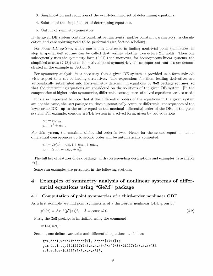
4.1 Computation of point symmetries of a third-order nonlinear ODE

As a first example, we find point symmetries of a third-order nonlinear ODE given by

y′′′(x) = Ax−3(y′′(x))3, A = const 6= 0. (4.2)

First, the GeM package is initialized using the command

with(GeM):

Second, one defines variables and differential equations, as follows.

gem_decl_vars(indeps=[x], deps=[Y(x)]);gem_decl_eqs([diff(Y(x),x,x,x)=A*x^(-3)*diff(Y(x),x,x)^3],solve_for=[diff(Y(x),x,x,x)]);

9

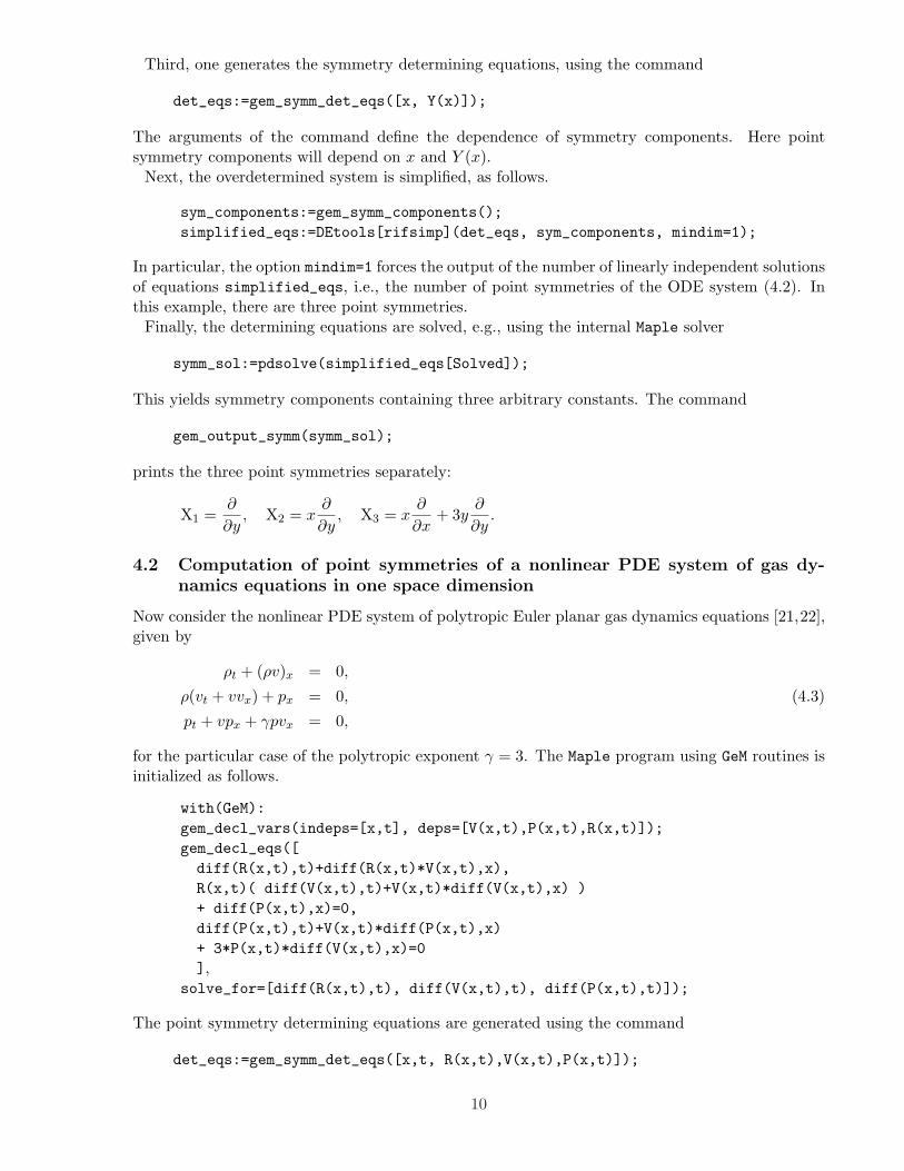
Third, one generates the symmetry determining equations, using the command

det_eqs:=gem_symm_det_eqs([x, Y(x)]);

The arguments of the command define the dependence of symmetry components. Here pointsymmetry components will depend on x and Y (x).

Next, the overdetermined system is simplified, as follows.

sym_components:=gem_symm_components();simplified_eqs:=DEtools[rifsimp](det_eqs, sym_components, mindim=1);

In particular, the option mindim=1 forces the output of the number of linearly independent solutionsof equations simplified_eqs, i.e., the number of point symmetries of the ODE system (4.2). Inthis example, there are three point symmetries.

Finally, the determining equations are solved, e.g., using the internal Maple solver

symm_sol:=pdsolve(simplified_eqs[Solved]);

This yields symmetry components containing three arbitrary constants. The command

gem_output_symm(symm_sol);

prints the three point symmetries separately:

X1 =∂

∂y, X2 = x

∂

∂y, X3 = x

∂

∂x+ 3y

∂

∂y.

4.2 Computation of point symmetries of a nonlinear PDE system of gas dy-namics equations in one space dimension

Now consider the nonlinear PDE system of polytropic Euler planar gas dynamics equations [21,22],given by

ρt + (ρv)x = 0,

ρ(vt + vvx) + px = 0,

pt + vpx + γpvx = 0,

(4.3)

for the particular case of the polytropic exponent γ = 3. The Maple program using GeM routines isinitialized as follows.

with(GeM):gem_decl_vars(indeps=[x,t], deps=[V(x,t),P(x,t),R(x,t)]);gem_decl_eqs([diff(R(x,t),t)+diff(R(x,t)*V(x,t),x),R(x,t)( diff(V(x,t),t)+V(x,t)*diff(V(x,t),x) )+ diff(P(x,t),x)=0,diff(P(x,t),t)+V(x,t)*diff(P(x,t),x)+ 3*P(x,t)*diff(V(x,t),x)=0],

solve_for=[diff(R(x,t),t), diff(V(x,t),t), diff(P(x,t),t)]);

The point symmetry determining equations are generated using the command

det_eqs:=gem_symm_det_eqs([x,t, R(x,t),V(x,t),P(x,t)]);

10

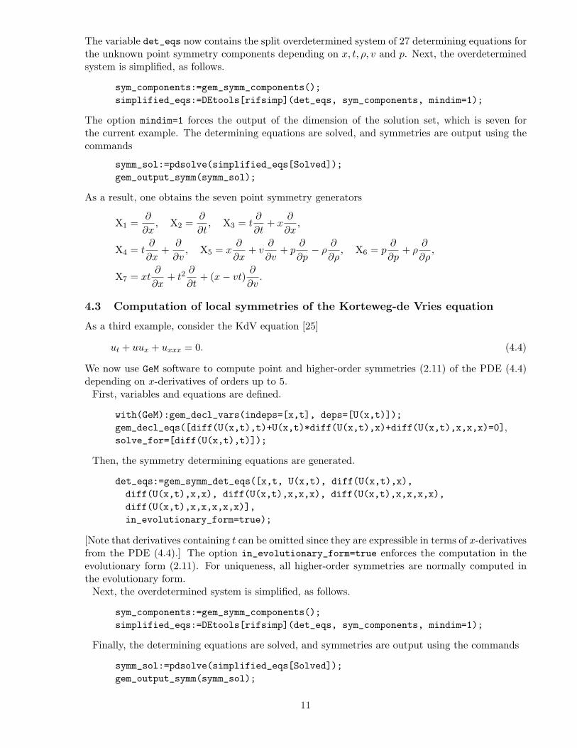
The variable det_eqs now contains the split overdetermined system of 27 determining equations forthe unknown point symmetry components depending on x, t, ρ, v and p. Next, the overdeterminedsystem is simplified, as follows.


The option mindim=1 forces the output of the dimension of the solution set, which is seven forthe current example. The determining equations are solved, and symmetries are output using thecommands

symm_sol:=pdsolve(simplified_eqs[Solved]);gem_output_symm(symm_sol);

As a result, one obtains the seven point symmetry generators

X1 =∂

∂x, X2 =

∂

∂t, X3 = t

∂

∂t+ x

∂

∂x,

X4 = t∂

∂x+

∂

∂v, X5 = x

∂

∂x+ v

∂

∂v+ p

∂

∂p− ρ

∂

∂ρ, X6 = p

∂

∂p+ ρ

∂

∂ρ,

X7 = xt∂

∂x+ t2

∂

∂t+ (x− vt)

∂

∂v.

4.3 Computation of local symmetries of the Korteweg-de Vries equation

As a third example, consider the KdV equation [25]

ut + uux + uxxx = 0. (4.4)

We now use GeM software to compute point and higher-order symmetries (2.11) of the PDE (4.4)depending on x-derivatives of orders up to 5.

First, variables and equations are defined.

with(GeM):gem_decl_vars(indeps=[x,t], deps=[U(x,t)]);gem_decl_eqs([diff(U(x,t),t)+U(x,t)*diff(U(x,t),x)+diff(U(x,t),x,x,x)=0],solve_for=[diff(U(x,t),t)]);

Then, the symmetry determining equations are generated.

det_eqs:=gem_symm_det_eqs([x,t, U(x,t), diff(U(x,t),x),diff(U(x,t),x,x), diff(U(x,t),x,x,x), diff(U(x,t),x,x,x,x),diff(U(x,t),x,x,x,x,x)],in_evolutionary_form=true);

[Note that derivatives containing t can be omitted since they are expressible in terms of x-derivativesfrom the PDE (4.4).] The option in_evolutionary_form=true enforces the computation in theevolutionary form (2.11). For uniqueness, all higher-order symmetries are normally computed inthe evolutionary form.

Next, the overdetermined system is simplified, as follows.


Finally, the determining equations are solved, and symmetries are output using the commands


11

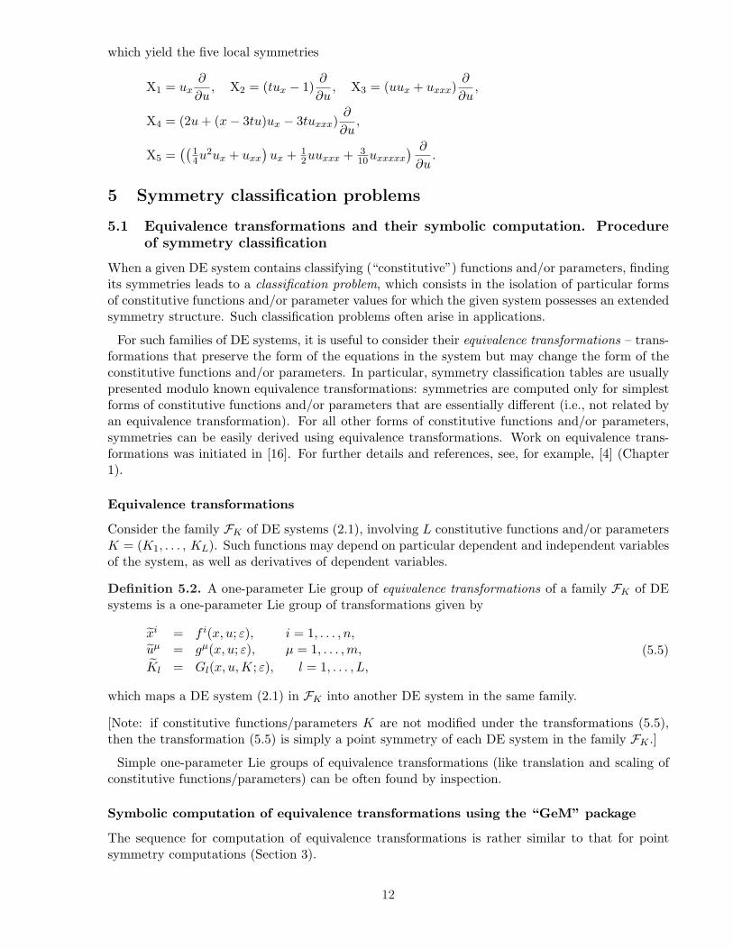
which yield the five local symmetries

X1 = ux∂

∂u, X2 = (tux − 1)

∂

∂u, X3 = (uux + uxxx)

∂

∂u,

X4 = (2u + (x− 3tu)ux − 3tuxxx)∂

∂u,

X5 =((

14u2ux + uxx

)ux + 1

2uuxxx + 310uxxxxx

) ∂

∂u.

5 Symmetry classification problems

5.1 Equivalence transformations and their symbolic computation. Procedureof symmetry classification

When a given DE system contains classifying (“constitutive”) functions and/or parameters, findingits symmetries leads to a classification problem, which consists in the isolation of particular formsof constitutive functions and/or parameter values for which the given system possesses an extendedsymmetry structure. Such classification problems often arise in applications.

For such families of DE systems, it is useful to consider their equivalence transformations – trans-formations that preserve the form of the equations in the system but may change the form of theconstitutive functions and/or parameters. In particular, symmetry classification tables are usuallypresented modulo known equivalence transformations: symmetries are computed only for simplestforms of constitutive functions and/or parameters that are essentially different (i.e., not related byan equivalence transformation). For all other forms of constitutive functions and/or parameters,symmetries can be easily derived using equivalence transformations. Work on equivalence trans-formations was initiated in [16]. For further details and references, see, for example, [4] (Chapter1).

Equivalence transformations

Consider the family FK of DE systems (2.1), involving L constitutive functions and/or parametersK = (K1, . . . , KL). Such functions may depend on particular dependent and independent variablesof the system, as well as derivatives of dependent variables.

Definition 5.2. A one-parameter Lie group of equivalence transformations of a family FK of DEsystems is a one-parameter Lie group of transformations given by

xi = f i(x, u; ε), i = 1, . . . , n,uµ = gµ(x, u; ε), µ = 1, . . . , m,

Kl = Gl(x, u, K; ε), l = 1, . . . , L,

(5.5)

which maps a DE system (2.1) in FK into another DE system in the same family.

[Note: if constitutive functions/parameters K are not modified under the transformations (5.5),then the transformation (5.5) is simply a point symmetry of each DE system in the family FK .]

Simple one-parameter Lie groups of equivalence transformations (like translation and scaling ofconstitutive functions/parameters) can be often found by inspection.

Symbolic computation of equivalence transformations using the “GeM” package

The sequence for computation of equivalence transformations is rather similar to that for pointsymmetry computations (Section 3).

12

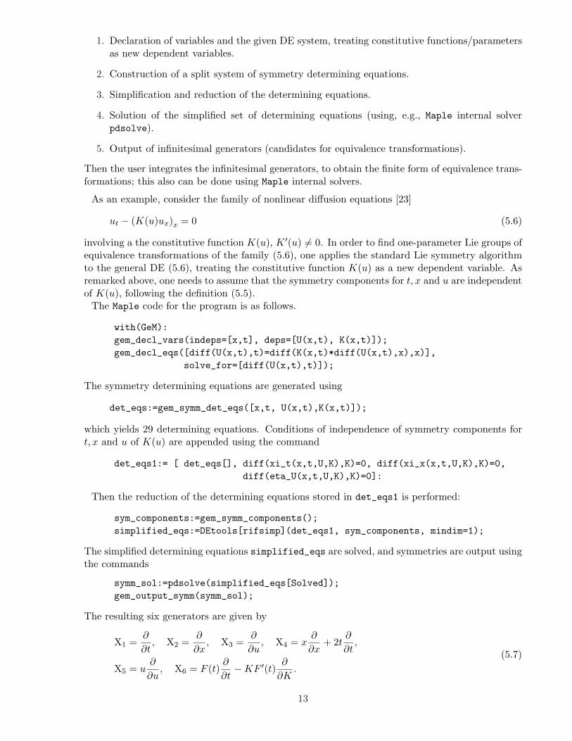
1. Declaration of variables and the given DE system, treating constitutive functions/parametersas new dependent variables.

2. Construction of a split system of symmetry determining equations.

3. Simplification and reduction of the determining equations.

4. Solution of the simplified set of determining equations (using, e.g., Maple internal solverpdsolve).

5. Output of infinitesimal generators (candidates for equivalence transformations).

Then the user integrates the infinitesimal generators, to obtain the finite form of equivalence trans-formations; this also can be done using Maple internal solvers.

As an example, consider the family of nonlinear diffusion equations [23]

ut − (K(u)ux)x = 0 (5.6)

involving a the constitutive function K(u), K ′(u) 6= 0. In order to find one-parameter Lie groups ofequivalence transformations of the family (5.6), one applies the standard Lie symmetry algorithmto the general DE (5.6), treating the constitutive function K(u) as a new dependent variable. Asremarked above, one needs to assume that the symmetry components for t, x and u are independentof K(u), following the definition (5.5).

The Maple code for the program is as follows.

with(GeM):gem_decl_vars(indeps=[x,t], deps=[U(x,t), K(x,t)]);gem_decl_eqs([diff(U(x,t),t)=diff(K(x,t)*diff(U(x,t),x),x)],

solve_for=[diff(U(x,t),t)]);

The symmetry determining equations are generated using

det_eqs:=gem_symm_det_eqs([x,t, U(x,t),K(x,t)]);

which yields 29 determining equations. Conditions of independence of symmetry components fort, x and u of K(u) are appended using the command

det_eqs1:= [ det_eqs[], diff(xi_t(x,t,U,K),K)=0, diff(xi_x(x,t,U,K),K)=0,diff(eta_U(x,t,U,K),K)=0]:

Then the reduction of the determining equations stored in det_eqs1 is performed:

sym_components:=gem_symm_components();simplified_eqs:=DEtools[rifsimp](det_eqs1, sym_components, mindim=1);

The simplified determining equations simplified_eqs are solved, and symmetries are output usingthe commands


The resulting six generators are given by

X1 =∂

∂t, X2 =

∂

∂x, X3 =

∂

∂u, X4 = x

∂

∂x+ 2t

∂

∂t,

X5 = u∂

∂u, X6 = F (t)

∂

∂t−KF ′(t)

∂

∂K.

(5.7)

13

One can check that for the generators X6 with the arbitrary function F (t), when F ′′(t) 6= 0 thetransformed function K is not a function of u only. Therefore these generators do not correspondto equivalence transformations of the family (5.6).

The finite form of the equivalence transformations of the family of PDEs (5.6) arises from the sixgenerators X1, . . . , X6 (F ′(t) = const) and therefore involves six arbitrary parameters. It is givenby

t = a4t + a1, x = a5x + a2, u = a6u + a3, K(u) =a2

5

a4K(u), (5.8)

where a1, . . . , a6 are arbitrary constants with a4a5a6 6= 0. In particular, under an equivalence trans-formation (5.8), a PDE system (5.6) with variables x, t, u and constitutive function K(u) is mapped

into a PDE system with variables x, t, u with the constitutive function K(u) =a2

5

a4K

(u− a3

a6

).

5.2 Symmetry classification procedure and its symbolic implementation

For DE systems involving constitutive functions and/or parameters, symmetry determining equa-tions are obtained as usual, using the algorithm described in Section 2.

After determining equations (2.13), (2.14) are obtained and split, the further reduction of theoverdetermined system essentially depends on the constitutive functions/parameters. Indeed, fortheir particular relations, such reduction may go differently and thus yield additional symmetries.Such relations or conditions for constitutive functions and/or parameters are called pivots, andformulated as pi(K, x, u) = 0, i = 1, 2, ....

Complete analysis of pivots and isolation of all different cases arising from different values ofpivots (case splitting) is effectively implemented in Maple’s rif package [17–19] and is used duringfor symmetry classification with GeM package.

The symmetry classification program that uses GeM package requires the execution of two programsequences.(i) Computation of equivalence transformations (Section 5.1).

(ii) Symmetry classification.

1. Declaration of variables and the given DE system. Constitutive functions/parameters aredeclared using special options freefunc=[...] and freeconst=[...] (see example in Section5.3 below).

2. Construction of a split system of symmetry determining equations.

3. Simplification and reduction of the overdetermined set of determining equations using rifsimp,with casesplit option for case splitting with respect to constitutive functions/parameters.

4. For each of the cases obtained in step 3:

(a) Choice of the simplest form of constitutive functions/parameters, using equivalencetransformations obtained above (by hand).

(b) Solution of the simplified set of determining equations, for the specific (chosen) form ofconstitutive functions/parameters.

(c) Output of symmetry generators in the given case.

In the above program sequence, as illustrated in the example in Section 5.3 below, step 4 has to beprogrammed separately for each case arising in step 3 which yields a different symmetry structure.The main reason for this intentional lack of automation is the utility of equivalence transformations

14

for the most compact presentation of the symmetry classification table. Indeed, for each classifi-cation case, solving pivot equations yields general forms of constitutive functions/parameters forthat case, which need to be put in the “simplest” form using equivalence transformations. Yet thenotion of “simplest” is hard to make algorithmic, hence case studies were left to the user.

Here it is worth remarking that though rifsimp-generated case trees are complete by construction,they can be redundant, presenting non-distinct cases as distinct ones in a non-obvious way. Anexcellent attempt to correct this minor deficiency using equivalence transformations was madein [26].

5.3 An example of point symmetry classification

As an example, consider the classification of point symmetries of the nonlinear diffusion equation(5.6) with respect to the constitutive function K(u) (K ′(u) 6= 0).

First, one defines variables using the commands

with(GeM):gem_decl_vars(indeps=[x,t], deps=[U(x,t)], freefunc=[K(U(x,t))]);

where the optional parameter freefunc=[...] is used to define arbitrary function(s). [Arbitraryconstants can be specified using another optional parameter freeconst=[...].]

The given equation (5.6) is defined using

gem_decl_eqs([diff(U(x,t),t)=diff(K(U(x,t))*diff(U(x,t),x),x)],solve_for=[diff(U(x,t),t)]);

The symmetry determining equations are generated using the command

det_eqs:=gem_symm_det_eqs([x,t, U(x,t)]);

which yields 10 determining equations.Next, one performs the automatic reduction and case splitting of the overdetermined linear PDE

system stored in det_eqs.

sym_components:=gem_symm_components();split_eqs:=DEtools[rifsimp](det_eqs, sym_components,

casesplit, mindim=1);

The Maple variable split_eqs now contains a table of different computed cases. The case tree canbe plotted using the command

caseplot(split_eqs,pivots);

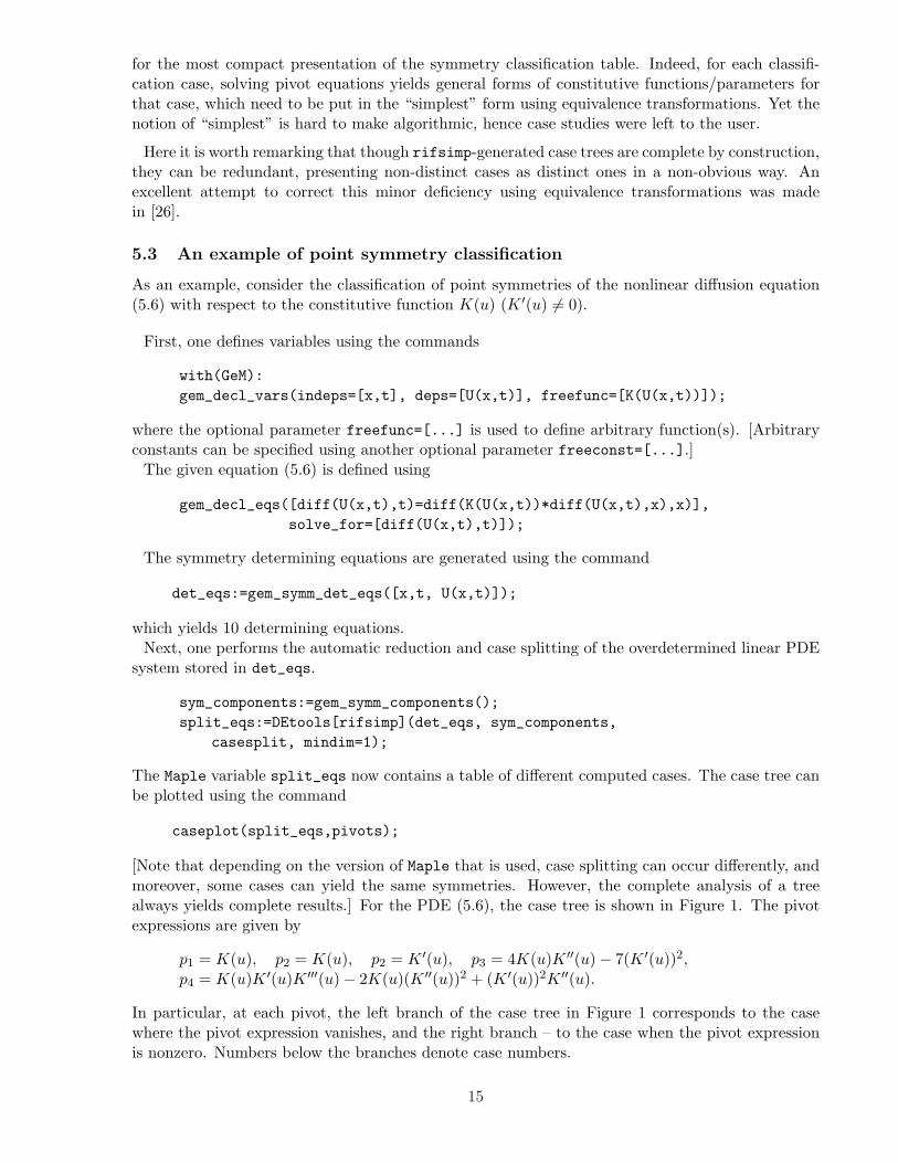
[Note that depending on the version of Maple that is used, case splitting can occur differently, andmoreover, some cases can yield the same symmetries. However, the complete analysis of a treealways yields complete results.] For the PDE (5.6), the case tree is shown in Figure 1. The pivotexpressions are given by

p1 = K(u), p2 = K(u), p2 = K ′(u), p3 = 4K(u)K ′′(u)− 7(K ′(u))2,p4 = K(u)K ′(u)K ′′′(u)− 2K(u)(K ′′(u))2 + (K ′(u))2K ′′(u).

In particular, at each pivot, the left branch of the case tree in Figure 1 corresponds to the casewhere the pivot expression vanishes, and the right branch – to the case when the pivot expressionis nonzero. Numbers below the branches denote case numbers.

15

Rif Case Tree

p3

p4

p2

p1

2

=

1

<>

<>

5

<>

<>

=

4

=

3

=

Figure 1: The tree of cases in the classification of point symmetries of the nonlinear diffusion equation (5.6).

For each case m in Figure 1 (1 ≤ q ≤ 5), the corresponding simplified set of determining equationsis accessed by calling split_eqs[q][Solved], and the number of independent solutions is givenby split_eqs[q][dimension].

Case 1. This is the most general case. Here one uses the commands

symm_sol:=pdsolve(split_eqs[1][Solved]);gem_output_symm(symm_sol);

which yield the three symmetries

X1 =∂

∂x, X2 =

∂

∂t, X3 = x

∂

∂x+ 2t

∂

∂t, (5.9)

holding for an arbitrary constitutive function K(u).

Case 2. In this case, the solution set has dimension four. This case is characterized by a restrictedODE satisfied by K(u), contained in split_eqs[2] [Solved]:

K ′′′(u) =2K(u)(K ′′(u))2 − (K ′(u))2K ′′(u)

K(u)K ′(u). (5.10)

One can show that modulo equivalence transformations (5.8), the equation (5.10) has two differentsolutions: K(u) = uν (ν = const) and K(u) = eu.

Case 2a. For K(u) = uν , one obtains the corresponding point symmetries using commands

case2a_symm_sol:=pdsolve(subs(K(U)=U^nu, split_system[2][Solved]));gem_output_symm(case2a_symm_sol);

This yields the three generic symmetries (5.9), and the additional symmetry

X4 = x∂

∂x+

2ν

u∂

∂u. (5.11)

16

Case 2b. For K(u) = eu, one uses commands

case2b_symm_sol:=pdsolve(subs(K(U)=exp(U), split_system[2][Solved]));gem_output_symm(case2b_symm_sol);

This yields the three generic symmetries (5.9), and the additional symmetry

X5 = x∂

∂x+ 2

∂

∂u. (5.12)

Case 3. In this case, the solution set has dimension five, and K(u) is restricted to satisfying theODE

K ′′(u) =74

(K ′(u))2

K(u). (5.13)

The general second-order ODE (5.13) involves two integration constants, both of which can beremoved using equivalence transformations (5.8). Thus modulo equivalence transformations, theonly solution of the equation (5.13) is K(u) = u−4/3. The corresponding point symmetries arecomputed using commands

case3_symm_sol:=pdsolve(subs(K(U)=U^(-4/3), split_system[3][Solved]));gem_output_symm(case3_symm_sol);

This yields the three symmetries (5.9), the symmetry (5.11) (with ν = −4/3), and the additionalsymmetry

X6 = x2 ∂

∂x− 3xu

∂

∂u. (5.14)

Cases 4 and 5. These cases correspond to linear diffusion equations (K(u) = const and K(u) = 0,respectively), and hence the PDE (5.6) has an infinite number of point symmetries in these cases.Indeed, split_eqs[q] [dimension] = ∞ for q = 4, 5. This completes the classification of pointsymmetries of the nonlinear diffusion equation (5.6).

Finally, the point symmetry classification of the nonlinear diffusion equation (5.6) is given inTable 1 [23].

Table 1: Point symmetry classification for the nonlinear diffusion equation (5.6).

K(u) # Point Symmetries

Arbitrary 3 X1 = ∂∂x

, X2 = ∂∂t

, X3 = x ∂∂x

+ 2t ∂∂t

.

uν 4 X1, X2, X3, X4 = x ∂∂x

+ 2νu ∂

∂u.

eu 4 X1, X2, X3, X5 = x ∂∂x

+ 2 ∂∂u

.

u−4/3 5 X1, X2, X3, X4

(ν = − 4

3

), X6 = x2 ∂

∂x− 3xu ∂

∂u.

17

6 Example of point symmetry classification of linear systems ofdifferential equations using “GeM” package

Consider the linear PDE system [24]

vt = ux, ut = c2(x)vx. (6.15)

for with dependent variables u(x, t), v(x, t), which is a potential system of a linear wave equation

utt = c2(x)uxx (6.16)

with variable wave speed c(x). We now use GeM package to classify nontrivial point symmetries of thesystem (6.15) with respect to the wave speed c(x), in the assumption c′(x) 6= 0. The classificationis done modulo the equivalence transformations of the system (6.15), which are computed in thesame way as shown in the example of Section 5.1, and are given by

t = a1a−15 t + a3v + a6, x = a1a5x + +a3u + a7,

u = a2a25u + a4x + a8, v = a2v + a4t + a9, c(x) = a2

5c(x),(6.17)

where a1, . . . , a9 are arbitrary constants with a1a2a5 6= 0.The variables and the equations are defined using the command

with(GeM):gem_decl_vars(indeps=[x,t], deps=[U(x,t),V(x,t)]);gem_decl_eqs([diff(U(x,t),t)=C(x)^2*diff(V(x,t),x), ,

diff(V(x,t),t)=diff(U(x,t),x)],solve_for=[diff(U(x,t),t), diff(V(x,t),t)]);

Then, the command

det_eqs:=gem_symm_det_eqs([ind, U(x,t), V(x,t)]);

is used to generate the ten determining equations (split with respect to derivatives vt, vx) and placethem into the variable det_eqs.

Next, similarly to the previous classification example, one performs the automatic reduction andcase splitting of the overdetermined linear PDE system stored in det_eqs.

sym_components:=gem_symm_components();split_eqs:=DEtools[rifsimp](det_eqs, sym_components, casesplit, mindim=1);

The Maple variable split_eqs now contains a table of different computed cases. The case tree isplotted using the command

caseplot(split_eqs,pivots);

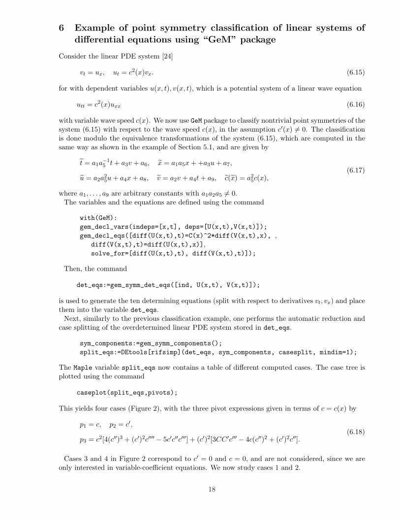
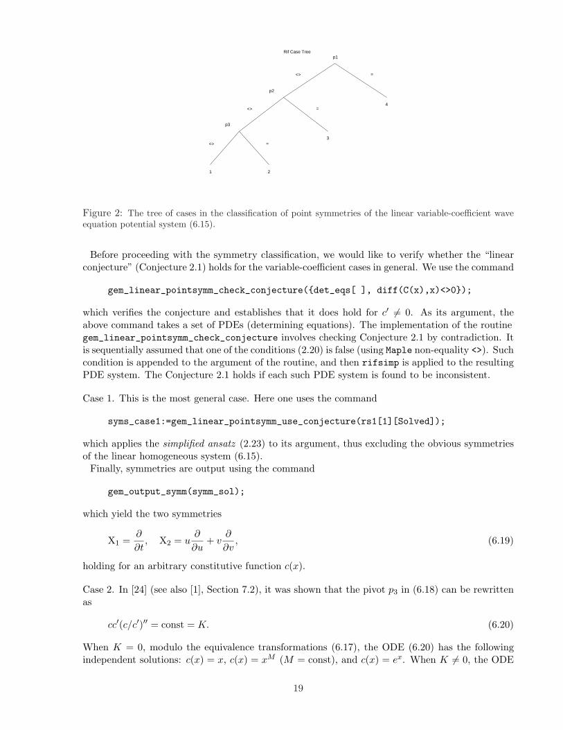
This yields four cases (Figure 2), with the three pivot expressions given in terms of c = c(x) by

p1 = c, p2 = c′,

p3 = c2[4(c′′)3 + (c′)2c′′′′ − 5c′c′′c′′′] + (c′)2[3CC ′c′′′ − 4c(c′′)2 + (c′)2c′′].(6.18)

Cases 3 and 4 in Figure 2 correspond to c′ = 0 and c = 0, and are not considered, since we areonly interested in variable-coefficient equations. We now study cases 1 and 2.

18

Rif Case Tree

p2

p3

p1

=

=

<>

=

<>

<>

4

3

2

1

Figure 2: The tree of cases in the classification of point symmetries of the linear variable-coefficient waveequation potential system (6.15).

Before proceeding with the symmetry classification, we would like to verify whether the “linearconjecture” (Conjecture 2.1) holds for the variable-coefficient cases in general. We use the command

gem_linear_pointsymm_check_conjecture({det_eqs[ ], diff(C(x),x)<>0});

which verifies the conjecture and establishes that it does hold for c′ 6= 0. As its argument, theabove command takes a set of PDEs (determining equations). The implementation of the routinegem_linear_pointsymm_check_conjecture involves checking Conjecture 2.1 by contradiction. Itis sequentially assumed that one of the conditions (2.20) is false (using Maple non-equality <>). Suchcondition is appended to the argument of the routine, and then rifsimp is applied to the resultingPDE system. The Conjecture 2.1 holds if each such PDE system is found to be inconsistent.

Case 1. This is the most general case. Here one uses the command

syms_case1:=gem_linear_pointsymm_use_conjecture(rs1[1][Solved]);

which applies the simplified ansatz (2.23) to its argument, thus excluding the obvious symmetriesof the linear homogeneous system (6.15).

Finally, symmetries are output using the command


which yield the two symmetries

X1 =∂

∂t, X2 = u

∂

∂u+ v

∂

∂v, (6.19)

holding for an arbitrary constitutive function c(x).

Case 2. In [24] (see also [1], Section 7.2), it was shown that the pivot p3 in (6.18) can be rewrittenas

cc′(c/c′)′′ = const = K. (6.20)

When K = 0, modulo the equivalence transformations (6.17), the ODE (6.20) has the followingindependent solutions: c(x) = x, c(x) = xM (M = const), and c(x) = ex. When K 6= 0, the ODE

19

(6.20) reduces to first-order ODEs; these cases are omitted here for brevity (for details, see [1],Section 7.2).

Case 2a: c(x) = x. Here we again use the command that employs the simplified ansatz (2.23):

syms_case1:=gem_linear_pointsymm_use_conjecture(rs1[2][Solved],free_func_form = [C(x)=x]);


which yields the two symmetries (6.19), and two additional symmetries

X3 = x∂

∂x+ u

∂

∂u,

X4 = 2 log(x)∂

∂t+ 2tx

∂

∂x+ (tu− xv)

∂

∂u−

(u

x+ tv

) ∂

∂v.

(6.21)

Case 2b: c(x) = xM , M 6= 0, 1. The simplified ansatz (2.23) here us used by the command

syms_case1:=gem_linear_pointsymm_use_conjecture(rs1[2][Solved],free_func_form = [C(x)=x^M,M<>0]);



X5 = (1−M)t∂

∂x+ x

∂

∂x+ Mu

∂

∂u,

X6 =((1−M)−1x2(1−M) + (1−M)t2

) ∂

∂t+ 2tx

∂

∂x

−(tu(1− 2M) + xv)∂

∂u− (

x1−2Mu + tu) ∂

∂v.

(6.22)

Case 2c: c(x) = ex. Here one uses a similar command

syms_case1:=gem_linear_pointsymm_use_conjecture(rs1[2][Solved],free_func_form = [C(x)=exp(x)]);



X7 = t∂

∂x− ∂

∂x− u

∂

∂u,

X8 =(t2 + e−2x

) ∂

∂t− 2t

∂

∂x+ (v − 2tu)

∂

∂u+ e−2xu

∂

∂v.

(6.23)

The symmetry classification results are summarized in Table 2.Following [1] (Section 7.2), we note that symmetries X4, X6, X8 yield nonlocal symmetries of the

linear wave equation (6.16), since the u-component of each of these symmetries essentially dependson the nonlocal variable v. For details on nonlocally related PDE systems, see [4], Chapter 3.

20

Table 2: Partial point symmetry classification for the potential system (6.15) for the linear waveequation (6.16).

c(x) # Point Symmetries

Arbitrary 2 X1 = ∂∂t

, X2 = u ∂∂u

+ v ∂∂v

.

x 4 X1, X2, X3 = x ∂∂x

+ u ∂∂u

, X4 = 2 log(x) ∂∂t

+ 2tx ∂∂x

+ (tu− xv) ∂∂u− (

ux

+ tv)

∂∂v

.

xM , 4 X1, X2, X5 = (1−M)t ∂∂x

+ x ∂∂x

+ Mu ∂∂u

,

M 6= 0, 1 X6 =((1−M)−1x2(1−M) + (1−M)t2

)∂∂t

+2tx ∂∂x− (tu(1− 2M) + xv) ∂

∂u− (

x1−2Mu + tu)

∂∂v

.

ex 4 X1, X2, X7 = t ∂∂x− ∂

∂x− u ∂

∂u, X8 =

(t2 + e−2x

)∂∂t− 2t ∂

∂x+ (v − 2tu) ∂

∂u+ e−2xu ∂

∂v.

7 Conclusions

Symbolic computations of symmetries of nonlinear and linear differential equations using the pack-age GeM for Maple were presented. Using routines of the GeM package, one can produce, split,simplify, and completely solve local symmetry determining equations for nonlinear and linear ODEand PDE systems and scalar equations, and output the basis of symmetry generators in a separatedform.

If a system of interest is a linear DE system, to perform a successful symbolic computation of itspoint symmetries, one often needs to exclude obvious point symmetries (2.17). [This is commonlythe case for linear PDE systems, which admit an infinite number of such trivial symmetries.] Formany linear DE systems, Conjecture 2.1 holds, which enables one to use the simplified symmetryform (2.21) which leads to effective exclusion of obvious point symmetries. In particular, for linearhomogeneous DEs, ansatz (2.23) can be used. For linear DE systems, a GeM package routine can beused that explicitly verifies Conjecture 2.1 using symbolic computations. If the conjecture holds,another routine employing the ansatz (2.23) for linear homogeneous DEs is available, which returnsonly nontrivial point symmetries. [Even for DE systems for which the conjecture does not hold, theroutine employing the simplified symmetry form still can be used, to provide a partial symmetryclassification.]

If the given DE system contains constitutive function(s) / parameter(s), a classification and casesplitting need to be performed. Symbolic implementations of symmetry classification and of therelated problem of computation of equivalence transformations are discussed and illustrated by anexample in Section 5.

It remains a practically important open question to formulate an explicit criterion to verifywhether or not the statement of Conjecture 2.1 holds for a given linear DE system.

AcknowledgementsThe author is grateful to NSERC for research support, and anonymous referees for helpful sug-

gestions.

References

[1] Bluman G.W. and Kumei S. Symmetries and Differential Equations. Applied Mathematical Sciences, No. 81.Springer-Verlag, New York, NY (1989).

[2] CRC Handbook of Lie Group Analysis of Differential Equations. (N.H. Ibragimov, ed.) Vol. 1. CRC Press, BocaRaton, Florida (1993).

[3] Bogoyavlenskij O. I. (2001). Infinite symmetries of the ideal MHD equilibrium equations. Phys. Lett. A 291(4-5), 256-264.

21

[4] Bluman G.W., Cheviakov A.F., and Anco S.C. Applications of Symmetry Methods to Partial Differential Equa-tions. Applied Mathematical Sciences, No. 168. Springer, New York (2010).

[5] Burde G.I. (2001). Potential symmetries of the nonlinear wave equation utt = (uux)x and related exact andapproximate solutions. J. Phys. A: Math. Gen. 34, 5355–5371.

[6] Wolf T. (2002a). Investigating differential equations with CRACK, LiePDE, Applysymm and ConLaw. In: Hand-book of Computer Algebra, Foundations, Applications, Systems (J. Grabmeier, E. Kaltofen, and V. Weispfenning,eds.). Springer, New York, NY, pp. 465–468.

[7] Temuerchaolu. (2003). An algorithmic theory of reduction of differential polynomial systems. Adv. Math. 32,208–220 (in Chinese).

[8] Hereman W. (1997). Review of symbolic software for Lie symmetry analysis, Math. Comp. Mod. 25, 115-132.

[9] Hereman W. (1996). Symbolic software for Lie symmetry analysis. In: CRC Handbook of Lie Group Analysis ofDifferential Equations , Vol. 3: New Trends in Theoretical Developments and Computational Methods, Chap.13, pp. 367–413. (N.H. Ibragimov, ed.) CRC Press, Boca Raton, FL (1996).

[10] Hereman W. (2005). Symbolic computation of conservation laws of nonlinear partial differential equations inmulti-dimensions. Int. J. Quant. Chem. 106, 278–299.

[11] Butcher J., Carminati J., and Vu K.T. (2003). A comparative study of the computer algebra packages whichdetermine the Lie point symmetries of differential equations. Comput. Phys. Commun. 155 (2), 92–114.

[12] Olver P.J. Applications of Lie Groups to Differential Equations. Springer, New York (1986).

[13] Cheviakov A. F. (2004). Bogoyavlenskij symmetries of ideal MHD equilibria as Lie point transformations. Phys.Lett. A. 321 (1), 34–49.

[14] Bluman G.W. (1990). Simplifying the form of Lie groups admitted by a given differential equation. J. Math.Anal. Appl. 145, 52–62.

[15] Ovsiannikov L.V. Group Properties of Differential Equations. Nauka, Novosibirsk (in Russian) (1962).

[16] Ovsiannikov L.V. Group Analysis of Differential Equations. Academic Press, New York (1982).

[17] Reid G.J., Wittkopf A.D., and Boulton A. (1996) Reduction of Systems of Nonlinear Partial Differential Equa-tions to Simplified Involutive Forms. Eur. J. Appl. Math. 7, 604-635.

[18] Reid G.J., Wittkopf A.D. (2000), Determination of Maximal Symmetry Groups of Classes of Differential Equa-tions. In: Proc. ISSAC 2000, ACM Press, 272–280.

[19] See Maple help system, sections on rifsimp,maxdimsys, and related commands.

[20] The GeM package and documentation is available at http://math.usask.ca/~cheviakov/gem/.

[21] Akhatov, I.S., Gazizov, R.K., and Ibragimov, N.H. (1987). Group classification of the equations of nonlinearfiltration. Sov. Math. Dokl. 35, 384–386.

[22] Bluman, G.W., Cheviakov A. F., and Ivanova N.M. (2006). Framework for nonlocally related PDE systems andnonlocal symmetries: extension, simplification, and examples. J. Math. Phys. 47, 113505.

[23] Ovsiannikov, L.V. (1959). Group properties of the nonlinear heat conduction equation. Dokl. Akad. Nauk USSR125, 492–495 (in Russian).

[24] Bluman G.W., Kumei S., and Reid G.J. (1988). New classes of symmetries for partial differential equations. J.Math. Phys. 29, 806–811.

[25] Korteweg D. J. and de Vries G. (1895). On the Change of Form of Long Waves Advancing in a RectangularCanal, and on a New Type of Long Stationary Waves. Philosophical Magazine 39, 422–443.

[26] Lisle I. and Huang T. S.-L. (2010) Algorithmic symmetry classification with invariance. J. Eng. Math. 66 (1-3),201–216.

22

symbolic computation of local symmetries of nonlinear and

Documents