symbolic and numeric computation in curve interrogation

Volume 14, (1995), number 1, pp. 25-34

Symbolic and Numeric Computation in Curve Interrogation

Gershon Elber

Computer Science Department, Technion, Israel Institute of Technology, Haifa 32000, Israel

Abstract The control of shape of curves is of great importance in computer aided geometric design. Determination of planar curves' convexity, the detection of infection points, coincident regions, and self intersection points, the enclosedarea of a closed curve, and the locations of extreme curvature are important features of curves that can affect the design, in modelling environments.

In this paper, we investigate the ability to robustly answer the above queries and related questions using an approach which exploits both symbolic computation and numeric analysis.

Keywords : Convexity, Curvature, Inflection points, Arc-length parameterization, Enclosed Area, Self-intersection.

1. Introduction

Freeform surfaces can be constructed in various ways. Predefined primitives and mechanical features can be represented using freeform surfaces. High level surface constructors, such as sweep, extrude, warp and bend1, constraint based modelling2-6, and low level direct manipulation of control points are all methods of surface construction and manipulation. In all those techniques, curves are used as intermediate representations in the process of a surface construction. Surfaces are frequently created by interpolating or approximating a set of curves. These curves can be explicitly supplied by the user, or can be implicitly created by the modelling system, when a high level surface constructor is invoked. It is therefore important to be able to create curves with shape controlled by constraints such as convexity, curvature, enclosed area, and no self intersections or inflection points.

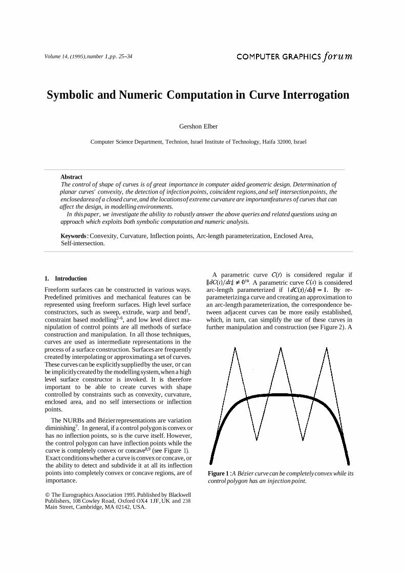
The NURBs and Bézier representations are variation diminishing7. In general, if a control polygon is convex or has no inflection points, so is the curve itself. However, the control polygon can have inflection points while the curve is completely convex or concave8,9 (see Figure 1). Exact conditions whether a curve is convex or concave, or the ability to detect and subdivide it at all its inflection points into completely convex or concave regions, are of importance.

A parametric curve is considered regular if A parametric curve is considered

arc-length parameterized if By re- parameterizing a curve and creating an approximation to an arc-length parameterization, the correspondence between adjacent curves can be more easily established, which, in turn, can simplify the use of these curves in further manipulation and construction (see Figure 2). A

Figure 1 : A Bézier curve can be completely convex while its control polygon has an injection point.

© The Eurographics Association 1995. Published by Blackwell Publishers, 108 Cowley Road, Oxford OX4 1JF, UK and 238 Main Street, Cambridge, MA 02142, USA.

26 G. Elber/Symbolic and Numeric Computation in Curve Interrogation

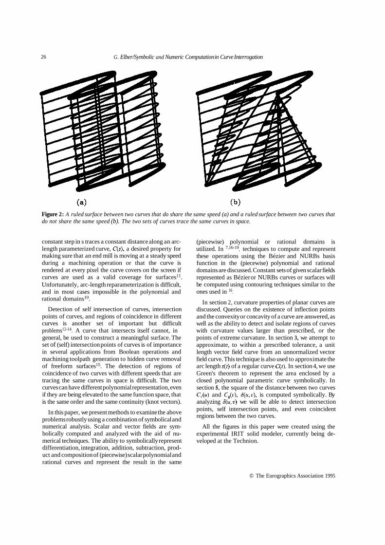
Figure 2: A ruled surface between two curves that do share the same speed (a) and a ruled surface between two curves that do not share the same speed (b). The two sets of curves trace the same curves in space.

constant step in s traces a constant distance along an arc- length parameterized curve, a desired property for making sure that an end mill is moving at a steady speed during a machining operation or that the curve is rendered at every pixel the curve covers on the screen if curves are used as a valid coverage for surfaces11. Unfortunately, arc-length reparameterization is difficult, and in most cases impossible in the polynomial and rational domains10.

Detection of self intersection of curves, intersection points of curves, and regions of coincidence in different curves is another set of important but difficult problems12-14. A curve that intersects itself cannot, in general, be used to construct a meaningful surface. The set of (self) intersection points of curves is of importance in several applications from Boolean operations and machining toolpath generation to hidden curve removal of freeform surfaces15. The detection of regions of coincidence of two curves with different speeds that are tracing the same curves in space is difficult. The two curves can have different polynomial representation, even if they are being elevated to the same function space, that is the same order and the same continuity (knot vectors).

(piecewise) polynomial or rational domains is utilized. In 7,16-19, techniques to compute and represent these operations using the Bézier and NURBs basis function in the (piecewise) polynomial and rational domains are discussed. Constant sets of given scalar fields represented as Bézier or NURBs curves or surfaces will be computed using contouring techniques similar to the ones used in 16.

In section 2, curvature properties of planar curves are discussed. Queries on the existence of inflection points and the convexity or concavity of a curve are answered, as well as the ability to detect and isolate regions of curves with curvature values larger than prescribed, or the points of extreme curvature. In section 3, we attempt to approximate, to within a prescribed tolerance, a unit length vector field curve from an unnormalized vector field curve. This technique is also used to approximate the arc length of a regular curve In section 4, we use Green's theorem to represent the area enclosed by a closed polynomial parametric curve symbolically. In section 5 , the square of the distance between two curves

and is computed symbolically. By analyzing we will be able to detect intersection points, self intersection points, and even coincident regions between the two curves.

In this paper, we present methods to examine the above problems robustly using a combination of symbolical and numerical analysis. Scalar and vector fields are symbolically computed and analyzed with the aid of numerical techniques. The ability to symbolically represent differentiation, integration, addition, subtraction, prod- uct and composition of (piecewise) scalar polynomial and rational curves and represent the result in the same

All the figures in this paper were created using the experimental IRIT solid modeler, currently being de- veloped at the Technion.

© The Eurographics Association 1995


Figure 3: Two examples of detection of inflection points of cubic planar Bspline curves with interior knots, using symbolic approach. the curvature sign scalar field is also shown for the respective curves. is at the interior knots (of multiplicity one) of the cubic curve.

2. Curvature Analysis of Curves

Curvature properties of curves are important for proper design. Most existing research attempts to derive conditions on the behavior of the curve such as inflection points, cusps, and convexity by deriving the necessary and sufficient conditions on the control polygon of the curve. Unfortunately, deriving these conditions is difficult and is usually for restricted cases only. In 20,21 only cubic polynomial curves are considered, whereas in 22 only uniform B-spline cubic curves are discussed. A different approach is taken herein by deriving the curvature scalar field symbolically, so it can be directly analyzed.

Let be a regular curve, that is The curvature of a is equal to 10,

where denotes the magnitude of a vector (L² norm) and is a unit vector in the curve's normal direction.

If is a planar curve, the magnitude of equation (1) can be simplified into,

is not representable as a rational because of the square root term in the denominators of both equations (1) and (2). However, the square of both equation (1) and equation (2) is computable and representable as a piecewise rational scalar curve, provided is a Bézier or a NURBs curve. Therefore, we consider The sign of directly indicates the convexity or concavity of the curve and is the same as the sign of the numerator in both equations (1) and (2), because the denominators are strictly positive for a regular curve. We define the sign function,

as a scalar field that preserves the sign of the curvature.



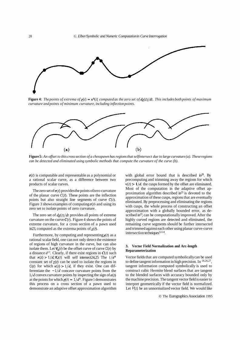
Figure 4: The points of extrema of computed as the zero set of This includes both points of maximum curvature and points of minimum curvature, including inflection points.

Figure 5: An offset to this cross section of a chesspawn has regions that selfintersect due to large curvature (a). These regions can be detected and eliminated using symbolic methods that compute the curvature of the curve (b).

is computable and representable as a polynomial or a rational scalar curve, as a difference between two products of scalar curves.

with global error bound that is described in28. By precomputing and trimming away the regions for which

the cusps formed by the offset are eliminated. Most of the computation in the adaptive offset approximation algorithm described in23 is devoted to the approximation of these cusps, regions that are eventually eliminated. By preprocessing and eliminating the regions with cusps, the whole process of constructing an offset approximation with a globally bounded error, as de-

The zero set of provides the points of zero curvature of the planar curve These points are the inflection points but also straight line segments of curve Figure 3 shows examples of computing and using its zero set to isolate points of zero curvature.

The zero set of provides all points of extreme curvature on the curve Figure 4 shows the points of extreme curvature, for a cross section of a pawn used in23, computed as the extrema points of

Furthermore, by computing and representing as a rational scalar field, one can not only detect the existence

scribed in23, can be computationally improved. After the highly curved regions are detected and eliminated, the remaining curve segments should be further intersected and trimmed against each other using planar curve-curve intersection techniques12-14.

of regions of high curvature in the curve, but can also isolate them. Let be the offset curve of curve by a distance d23. Clearly, if there exist regions in such that will self intersect24,25 The constant set of can be used to isolate the regions in

for which if they exist. One can dif- ferentiate the - concave curvature points from the

convex curvature points by inspecting the sign of at the points for which Figure 5 demonstrates this process on a cross section of a pawn used to demonstrate an adaptive offset approximation algorithm

3. Vector Field Normalization and Arc-length Reparameterization

Vector fields that are computed symbolically can be used to define tangent information in high precision. In 18,26,27, tangent information computed symbolically is used to construct cubic Hermite blend surfaces that are tangent to the blended surfaces with accuracy bounded only by the machine precision. The tangent vector field is easier to interpret geometrically if the vector field is normalized. Let be an unnormalized vector field. We would like


G. Elber/Symbolic and Numeric Computation in Curve Interrogation 29

to be able to approximate the unit length vector field of to within a given tolerance, such that and

are collinear and is unit length if Although is not representable as a

polynomial or rational, in general, is and is equal to,

Let M(t) be a scalar field defined using m(t), with the same order and continuity (knot vector), by substituting each coefficient k in the control polygon of m(t) as in the control polygon of M(t).

The error between a continuous function and its Schoenberg variation diminishing spline approximationz8

over a knot vector is where By using a sequence of Schoenberg variation

diminishing spline approximations to each one

The construction of M(t) from m(t) is the only numeric stage (1) in Algorithm 1 . M(t) can be constructed by sampling m(t) at the node values of M(t) and setting the coefficients of M(t) to be at these points. As a Schoenberg variation diminishing spline, M(t) will converge using refinement to the inverse of the square root of the magnitude, guaranteeing the convergence of the entire algorithm.

In step (2) of Algorithm 1, the convex hull property of the Bézier and NURBs representations can be exploited to compute bounds on by inspecting the coefficients of

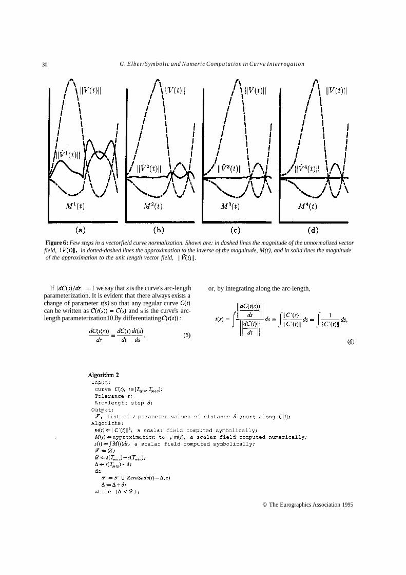
Figure 6 shows an example of this approach and demonstrates the effect of the refinement on the con-

based on a knot vector that is a refinement of the previous one, and a sequence, of refined representations of V(t), based on the same sequence of knot vectors, we form a converging sequence of approximations to Using the refinement sequence the sequence converges to Let

By suitable refinement on can converge as closely as needed to the exact unit length vector field. By inspecting we can not only determine the quality of the approximation but also figure out the regions in the curve that has error larger than allowed and apply refinement to only these regions.

An iterative algorithm that adaptively refines a vector field, at the regions with large error and approximates a unit length vector field, with the desired tolerance so that can now be derived.

vergence. were computed from the original quadratic Bspline curve, V(t), which has one interior knot. In Figures 6(b) to (d), 3, 6, and 12 new knots were inserted, respectively, into the parametric domain of V(t).

Table 1: Convergence of to a unit length using refinement


30 G. Elber/Symbolic and Numeric Computat ion in Curve Interrogation

Figure 6: Few steps in a vectorfield curve normalization. Shown are: in dashed lines the magnitude of the unnormalized vector field, in dotted-dashed lines the approximation to the inverse of the magnitude, M(t), and in solid lines the magnitude of the approximation to the unit length vector field,

If we say that s is the curve's arc-length parameterization. It is evident that there always exists a change of parameter t(s) so that any regular curve can be written as and s is the curve's arc- length parameterization10. By differentiating :

or, by integrating along the arc-length,


G. Elber/Symbolic and Numeric Computation in Curve Interrogation 31

Figure 7: Two examples of an approximation of arc-length reparameterization of curves. In (a), constant steps along the original parameterization are shown while in (b) the arc-length steps computed using Algorithm 2 are displayed.

because Because is regular, The integration of a strictly positive function yields a strictly increasing function, t(s).

Unfortunately, equation (6) is an integration with respect to the arc length parameter s which is unknown. Instead, the following approximation approach to arc length is used.

behaviour. If is a polynomial planar curve, one can exploit Green’s theorem and the symbolic tools defined herein to yield a symbolic closed form formulation of the enclosed area, represented as a scalar field.

Given continuous functions the Green’s theorem for a simple closed curve C,

can be computed symbolically. can be numerically approximated from using the same technique that is described in Algorithm 1. Integration can also be computed symbolically for polynomial Bezier and Bspline curves (see 7).

An algorithm to step along an arbitrary regular curve with constant arc-length steps can now be derived. (Algorithm 2 , where uses numerical methods to find the zero set of c(t) to within )

Figure 7 shows some examples of the approach taken in Algorithm 2 to create constant arc-length steps along curves.

4. Enclosed Area of Closed Curves

It is common to attempt and design a complicated surface, such as a fuselage of a plane or a ship hull, by defining a set of cross sections that the surface interpolates or approximates. It is important to be able to compute the enclosed area of such a cross section, or even guarantee that all cross sections have certain areas, since these areas directly affect the volume that will be confined by the designed surface, and its hydro/aerodynamic

where is the enclosed area by the closed curve C(t).

hand side of equation (8) becomes or, Let and let Then the right

In parametric form equation (9) is equal to,

Equation (10) is computable and representable using the symbolic tools assumed in section 1. One can compute and represent the (area) integral of a closed polynomial curve as a polynomial7, while the area itself is the definite integral evaluated at the two parameter values of the curve’s end points.

5. Curve Curve Intersection and Coincidence

The need to find the intersection points of two curves rises in numerous instances, including modeling, Boolean operations, machining toolpath generation, and hidden curve removal of freeform surfaces16. Moreover, the detection of coincidence of regions of curves that trace the same geometry in a different speed is a difficult problem. By representing the distance function sym-


32 G. Elber / Symbolic and Numeric Computation in Curve Interrogation

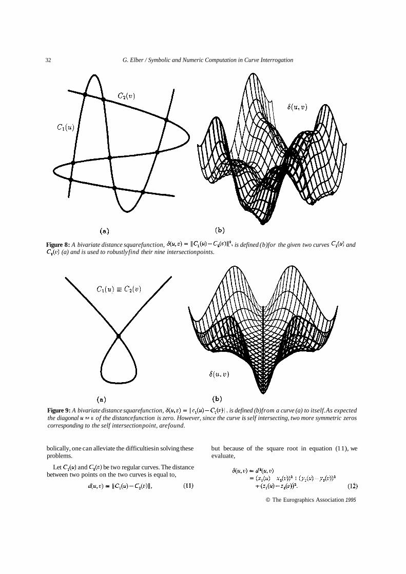
Figure 8: A bivariate distance square function, is defined (b) for the given two curves and (a) and is used to robustly find their nine intersection points.

Figure 9: A bivariate distance square function, is defined (b) from a curve (a) to itself. As expected the diagonal of the distance function is zero. However, since the curve is self intersecting, two more symmetric zeros corresponding to the self intersection point, are found.

bolically, one can alleviate the difficulties in solving these problems. evaluate,

but because of the square root in equation (1 1), we

Let and be two regular curves. The distance between two points on the two curves is equal to,


G. Elber/ Symbolic and Numeric Computation in Curve Interrogation 33

Clearly is computable and representable as a polynomial or rational scalar field because the and

coefficients can be rewritten as and respectively. Figures 8 and 9 provide two examples of

the distance function.

By using bivariate minimization methods, solutions to the intersection points can be robustly found. Further- more, not only can one find the curve’s intersection points, but the closest points or the points with largest distance on the two curves can be isolated in the same way, by finding the local minima or maxima of A search for local extrema of an explicit surface, as is, can be mapped to a zero set search on a different explicit surface,

In general and at an intersection point, If is continuous, and using the convex

hull property of the Bézier and NURBs representations, it is clear that at the neighborhood of an intersection point, there exists a non positive coefficient in the control mesh of

In Figures 8 and 9, a simple subdivision based algorithm is used. This subdivides a surface if one of its coefficients is non positive, until a termination criterion is reached, usually that the size of the parametric domain is sufficiently small. This simple algorithm was found reasonably fast and very robust.

By elevating the curve curve intersection problem a dimension, the problem is transformed into a zero set finding problem. One can use not only to robustly find the (self) intersection points and shortest distance points, but also to find regions of coincidence manifested as local minima curves on that are everywhere zero as well. Further, the isolation of the regions in such that for some constant is reduced to the computation of the zero set of

6. Conclusion

We have shown that few symbolic tools can enhance the robustness of current analysis methods of freeform curves as well as introduce new analysis techniques altogether. It is clear that the examples that were demonstrated in this paper are only a small subset of problems that can benefit from this symbolic approach and further research in the area is to be carried out.

References

1. B. Cobb, “Design of Sculptured Surfaces Using The B-spline Representation, ” Ph.D. Thesis, University of Utah, Computer Science Department (1984).

G. Celniker, “Shape Wright: Finite Element Based 2.

3.

4.

5.

6.

7.

8.

9.

10.

11.

12.

13.

14.

15.

16.

Free-Form Shape Design,” Ph.D. Thesis, Masachusetts Institute of Technology, Mechanical Engineering (1990).

G. Celniker and W. Welch, “Linear Constraints for Deformable B-spline Surfaces, ” Computer Graphics (Symposium on Interactive 3D graphics), 25(2), pp.

Y. Hel-Or, A. Rappoport and M. Werman, “ Relaxed Parametric Design with Probabilistic Constraints, ” 2nd A C M Solid Modeling Conference, pp. 261-270, Montreal Canada (1993).

M. Kallay, “ Constrainted Optimization in Surface Design,” Modeling in Computer Graphics, B. Falcidieno and T.L. Kunii (Eds.), Working Confer- ence on Geometric Modeling in Computer Graphics (IFIP TC 5/WG 5.10), Genova (1993).

W. Welch and A. Witkin, “Variational Surface Modeling, ” Computer Graphics (Siggraph 1992),

G. Farin, ‘‘ Curves and Surfaces for Computer Aided Geometric Design, ” Academic Press, Inc. Third Edition (1993).

J.A. Roulier, “ Bézier curves of Positive Curvature, ” Computer Aided Geometric Design, 5, pp. 59-70 (1988).

N.S. Sapidis, “Controlling the Curvature of a Quadratic Bézier curve,” Computer Aided Geometric Design, 9, pp. 85-91 (1992).

M.P. DoCarmo, Differential Geometry of Curves and Surfaces, Prentice-Hall(1976).

G. Elber and E. Cohen, “Adaptive Isocurves Based Rendering for Freeform Surfaces, ” Technical Report UUCS-92-040, University of Utah (1992).

M. Markot and R.L. Magenson, “Solutions of Tan- gential Surface and Curve Intersections, ” Computer Aided Design, 21(7), pp. 421-429 (1989).

T.W. Sederberg and S. Parry, “Comparison of Three Curve Intersection Algorithms, ” Computer Aided Design, 18(1), pp. 58-63 (1986).

T.W. Sederberg and T. Nishita, “Curve Intersection using Bezier Clipping, ” Computer Aided Design,

G. Elber and E. Cohen, “Hidden Curve Removal for Free Form Surfaces, ” Computer Graphics (Siggraph 1990), 24(4), pp. 95-104 (1990).

G. Elber, “Free Form Surface Analysis using a Hybrid of Symbolic and Numeric Computation, ” Ph.D. thesis, University of Utah, Computer Science Department (1992).

165-170 (1992).

26(2) pp. 157-166 (1992).

22(4), pp. 538-549 (1990).



17. R.T. Farouki and V.T. Rajan, “Algorithms for Polynomials in Bernstein Form, ” Computer Aided Geometric Design, 5, pp. 1-26 (1988).

18. K. Kim, “ Blending Parametric Surfaces, ” M.S. Thesis, University of Utah, Computer Science De- partment (1992).

19. K. Morken, “Some Identities for Products and Degree Raising of Splines,” To appear in the Journal of Constructive Approximation.

20. D.S. Kim, “Hodograph Approach to Geometric Characterization of Parametric Cubic Curves, ” Computer Aided Design, 25(10), pp. 644-654 (1993).

21. M.C. Stone and T.D. DeRose, “A Geometric Characterization of Parametric Cubic Curves, ” ACM Transactions on Graphics, 8(3), pp. 147-163 (1989).

22. E. Kantorowitz and Y. Schechner, “Managing the Shape of Planar Splines by Their Control Polygons, ” Computer Aided Design, 25(6), pp. 355-364 (1993).

23. G. Elber and E. Cohen, “Error Bounded Variable Distance Offset Operator for Free Form Curves and Surfaces, ” International Journal of Computational Geometry and Applications, 1(1), pp. 67-78 (1991).

24. G. Elber and E. Cohen, “Error Bounded Variable Distance Offset Operator for Free Form Curves and Surfaces,” Technical Report UUCS-91-001, Uni- versity of Utah (1992).

25. R.T. Farouki and C.A. Neff, “Some Analytic and Algebraic Properties of Plane Offset Curves,” Re- search Report 14364 (#64329) 1/25/89, IBM Re- search Division.

26. D.J. Fillip, “Blending Parametric Surfaces,” ACM Transaction on Graphics, 8(3), pp. 165-173 (1989).

27. P. Koparkar, “Parametric Blending using Fanout Surfaces, ” Symposium on Solid Modeling Foundation and CAD/CAM Applications, Austin Texas, pp.

28. M. Marsden and I.J. Schoenberg, “On Variation Diminishing Spline Approximation Methods, ” Mathematica, 8(31) 1 , pp. 61-82 (1966).

317-327 (1991).


symbolic and numeric computation in curve interrogation

Documents