symbolic algorithms for qualitative analysis of …nisarg/papers/symbolicmdp.fmsd.pdfform methods...

Form Methods Syst Des (2013) 42:301–327DOI 10.1007/s10703-012-0180-2

Symbolic algorithms for qualitative analysis of Markovdecision processes with Büchi objectives

Krishnendu Chatterjee · Monika Henzinger ·Manas Joglekar · Nisarg Shah

Published online: 13 December 2012© Springer Science+Business Media New York 2012

Abstract We consider Markov decision processes (MDPs) with Büchi (liveness) objec-tives. We consider the problem of computing the set of almost-sure winning states fromwhere the objective can be ensured with probability 1. Our contributions are as follows:First, we present the first subquadratic symbolic algorithm to compute the almost-sure win-ning set for MDPs with Büchi objectives; our algorithm takes O(n · √

m) symbolic stepsas compared to the previous known algorithm that takes O(n2) symbolic steps, where n isthe number of states and m is the number of edges of the MDP. In practice MDPs haveconstant out-degree, and then our symbolic algorithm takes O(n · √

n) symbolic steps, ascompared to the previous known O(n2) symbolic steps algorithm. Second, we present a newalgorithm, namely win-lose algorithm, with the following two properties: (a) the algorithmiteratively computes subsets of the almost-sure winning set and its complement, as com-pared to all previous algorithms that discover the almost-sure winning set upon termination;and (b) requires O(n · √

K) symbolic steps, where K is the maximal number of edges ofstrongly connected components (scc’s) of the MDP. The win-lose algorithm requires sym-bolic computation of scc’s. Third, we improve the algorithm for symbolic scc computation;the previous known algorithm takes linear symbolic steps, and our new algorithm improves

The research was supported by Austrian Science Fund (FWF) Grant No P 23499-N23 on Modern GraphAlgorithmic Techniques in Formal Verification, FWF NFN Grant No S11407-N23 (RiSE), ERC Startgrant (279307: Graph Games), and Microsoft faculty fellows award.

A preliminary version of the paper appeared in Computer Aided Verification (CAV), 2011.

K. Chatterjee (�)IST Austria, Klosterneuburg, Austriae-mail: [email protected]

M. HenzingerUniversity of Vienna, Vienna, Austria

M. JoglekarStanford University, Palo Alto, USA

N. ShahCarnegie Mellon University, Pittsburgh, USA

mailto:[email protected]

302 Form Methods Syst Des (2013) 42:301–327

the constants associated with the linear number of steps. In the worst case the previousknown algorithm takes 5 · n symbolic steps, whereas our new algorithm takes 4 · n symbolicsteps.

Keywords Markov decision processes · Probabilistic verification · Büchi objectives ·Symbolic algorithms

1 Introduction

Markov decision processes The standard model of systems in verification of probabilisticsystems is Markov decision processes (MDPs) that exhibit both probabilistic and nonde-terministic behavior [13]. MDPs have been used to model and solve control problems forstochastic systems [11]: there, nondeterminism represents the freedom of the controller tochoose a control action, while the probabilistic component of the behavior describes thesystem response to control actions. MDPs have also been adopted as models for concurrentprobabilistic systems [7], probabilistic systems operating in open environments [19], andunder-specified probabilistic systems [2]. A specification describes the set of desired behav-iors of the system, which in the verification and control of stochastic systems is typically anω-regular set of paths. The class of ω-regular languages extends classical regular languagesto infinite strings, and provides a robust specification language to express all commonly usedspecifications, such as safety, liveness, fairness, etc. [24]. Parity objectives are a canonicalway to define such ω-regular specifications. Thus MDPs with parity objectives provide thetheoretical framework to study problems such as the verification and control of stochasticsystems.

Qualitative and quantitative analysis The analysis of MDPs with parity objectives can beclassified into qualitative and quantitative analysis. Given an MDP with parity objective, thequalitative analysis asks for the computation of the set of states from where the parity objec-tive can be ensured with probability 1 (almost-sure winning). The more general quantitativeanalysis asks for the computation of the maximal probability at each state with which thecontroller can satisfy the parity objective.

Importance of qualitative analysis The qualitative analysis of MDPs is an important prob-lem in verification that is of interest irrespective of the quantitative analysis problem. Thereare many applications where we need to know whether the correct behavior arises with prob-ability 1. For instance, when analyzing a randomized embedded scheduler, we are interestedin whether every thread progresses with probability 1 [9]. Even in settings where it sufficesto satisfy certain specifications with probability p < 1, the correct choice of p is a chal-lenging problem, due to the simplifications introduced during modeling. For example, inthe analysis of randomized distributed algorithms it is quite common to require correctnesswith probability 1 (see, e.g., [16, 17, 23]). Furthermore, in contrast to quantitative analysis,qualitative analysis is robust to numerical perturbations and modeling errors in the transitionprobabilities, and consequently the algorithms for qualitative analysis are combinatorial. Fi-nally, for MDPs with parity objectives, the best known algorithms and all algorithms usedin practice first perform the qualitative analysis, and then perform a quantitative analysis onthe result of the qualitative analysis [6–8]. Thus qualitative analysis of MDPs with parityobjectives is one of the most fundamental and core problems in verification of probabilis-tic systems. One of the key challenges in probabilistic verification is to obtain efficient andsymbolic algorithms for qualitative analysis of MDPs with parity objectives, as symbolicalgorithms allow to handle MDPs with a large state space.

Form Methods Syst Des (2013) 42:301–327 303

Previous results The qualitative analysis of MDPs with parity objectives is achieved by it-eratively applying solutions of the qualitative analysis of MDPs with Büchi objectives [6–8].The qualitative analysis of an MDP with a parity objective with d priorities can be achievedby O(d) calls to an algorithm for qualitative analysis of MDPs with Büchi objectives, andhence we focus on the qualitative analysis of MDPs with Büchi objectives. The classicalalgorithm for qualitative analysis of MDPs with Büchi objectives works in O(n · m) time,where n is the number of states, and m is the number of edges of the MDP [7, 8]. The classi-cal algorithm can be implemented symbolically, and it takes at most O(n2) symbolic steps.An improved algorithm for the problem was given in [5] that works in O(m · √

m) time.The algorithm of [5] crucially depends on maintaining the same number of edges in certainforward searches. Thus the algorithm needs to explore edges of the graph explicitly andis inherently non-symbolic. A recent O(m · n2/3) time algorithm for the problem was givenin [4]; however the algorithm requires the dynamic-tree data structure of Sleator-Tarjan [20],and such data structures cannot be implemented symbolically. In the literature, there is nosymbolic subquadratic algorithm for qualitative analysis of MDPs with Büchi objectives.

Our contribution In this work our main contributions are as follows.

1. We present a new and simpler subquadratic algorithm for qualitative analysis of MDPswith Büchi objectives that runs in O(m · √m) time, and show that the algorithm can beimplemented symbolically. The symbolic algorithm takes at most O(n · √

m) symbolicsteps, and thus we obtain the first symbolic subquadratic algorithm. In practice, MDPsoften have constant out-degree: for example, see [10] for MDPs with large state spacebut constant number of actions, or [11, 18] for examples from inventory managementwhere MDPs have constant number of actions (the number of actions corresponds to theout-degree of MDPs). For MDPs with constant out-degree our new symbolic algorithmtakes O(n · √

n) symbolic steps, as compared to O(n2) symbolic steps of the previousbest known algorithm.

2. All previous algorithms for the qualitative analysis of MDPs with Büchi objectives it-eratively discover states that are guaranteed to be not almost-sure winning, and onlywhen the algorithm terminates the almost-sure winning set is discovered. We present anew algorithm (namely win-lose algorithm) that iteratively discovers both states in thealmost-sure winning set and its complement. Thus if the problem is to decide whether agiven state s is almost-sure winning, and the state s is almost-sure winning, then the win-lose algorithm can stop at an intermediate iteration unlike all the previous algorithms.Our algorithm works in time O(

√KE · m) time, where KE is the maximal number of

edges of any scc of the MDP (in this paper we write scc for maximal strongly connectedcomponent). We also show that the win-lose algorithm can be implemented symbolically,and it takes at most O(

√KE · n) symbolic steps.

3. Our win-lose algorithm requires to compute the scc decomposition of a graph in O(n)

symbolic steps. The scc decomposition problem is one of the most fundamental problemin the algorithmic study of graph problems. The symbolic scc decomposition problem hasmany other applications in verification: for example, checking emptiness of ω-automata,and bad-cycle detection problems in model checking, see [3] for other applications. AnO(n · logn) symbolic step algorithm for scc decomposition was presented in [3], andthe algorithm was improved in [12]. The algorithm of [12] is a linear symbolic step sccdecomposition algorithm that requires at most min{5 · n,5 · D · N + N} symbolic steps,where D is the diameter of the graph, and N is the number of scc’s of the graph. Wepresent an improved version of the symbolic scc decomposition algorithm. Our algorithmimproves the constants of the number of the linear symbolic steps. Our algorithm requires


at most min{3 ·n+N,5 ·D∗ +N} symbolic steps, where D∗ is the sum of the diameters ofthe scc’s of the graph. Thus, in the worst case, the algorithm of [12] requires 5 ·n symbolicsteps, whereas our algorithm requires 4 · n symbolic steps. Moreover, the number ofsymbolic steps of our algorithm is always bounded by the number of symbolic steps ofthe algorithm of [12] (i.e. our algorithm is never worse).

Our experimental results show that our new algorithms perform better than the previousknown algorithms both for qualitative analysis of MDPs with Büchi objectives and symbolicscc computation.

2 Definitions

Markov decision processes (MDPs) A Markov decision process (MDP) G = ((S,E),

(S1, SP ), δ) consists of a directed graph (S,E), a partition (S1, SP ) of the finite set S ofstates, and a probabilistic transition function δ : SP → D(S), where D(S) denotes the setof probability distributions over the state space S. The states in S1 are the player-1 states,where player 1 decides the successor state, and the states in SP are the probabilistic (orrandom) states, where the successor state is chosen according to the probabilistic transi-tion function δ. We assume that for s ∈ SP and t ∈ S, we have (s, t) ∈ E iff δ(s)(t) > 0,and we often write δ(s, t) for δ(s)(t). For a state s ∈ S, we write E(s) to denote the set{t ∈ S | (s, t) ∈ E} of possible successors. For technical convenience we assume that everystate in the graph (S,E) has at least one outgoing edge, i.e., E(s) �= ∅ for all s ∈ S. We willdenote by n = |S| and m = |E| the size of the state space and the number of transitions (oredges), respectively.

Plays and strategies An infinite path, or a play, of an MDP G is an infinite sequenceω = 〈s0, s1, s2, . . .〉 of states such that (sk, sk+1) ∈ E for all k ∈ N. We write Ω for the setof all plays, and for a state s ∈ S, we write Ωs ⊆ Ω for the set of plays that start from thestate s. A strategy for player 1 is a function σ : S∗ · S1 → D(S) that chooses the probabilitydistribution over the successor states for all finite sequences w ∈ S∗ · S1 of states endingin a player-1 state (the sequence represents a prefix of a play). A strategy must respectthe edge relation: for all w ∈ S∗ and s ∈ S1, if σ(w · s)(t) > 0, then t ∈ E(s). A strategy isdeterministic (pure) if it chooses a unique successor for all histories (rather than a probabilitydistribution), otherwise it is randomized. Player 1 follows the strategy σ if in each player-1move, given that the current history of the play is w ∈ S∗ · S1, she chooses the next stateaccording to σ(w). We denote by Σ the set of all strategies for player 1. A memorylessplayer-1 strategy does not depend on the history of the play but only on the current state;i.e., for all w,w′ ∈ S∗ and for all s ∈ S1 we have σ(w · s) = σ(w′ · s). A memoryless strategycan be represented as a function σ : S1 → D(S), and a pure memoryless strategy can berepresented as σ : S1 → S.

Once a starting state s ∈ S and a strategy σ ∈ Σ is fixed, the outcome of the MDP is arandom walk ωσ

s for which the probabilities of events are uniquely defined, where an eventA ⊆ Ω is a measurable set of plays. For a state s ∈ S and an event A ⊆ Ω , we write Prσs (A)

for the probability that a play belongs to A if the game starts from the state s and player 1follows the strategy σ .

Objectives We specify objectives for player 1 by providing a set of winning plays Φ ⊆ Ω .We say that a play ω satisfies the objective Φ if ω ∈ Φ . We consider ω-regular objec-tives [24], specified as parity conditions. We also consider the special case of Büchi objec-tives.


– Büchi objectives. Let T be a set of target states. For a play ω = 〈s0, s1, . . .〉 ∈ Ω , we defineInf(ω) = {s ∈ S | sk = s for infinitely many k} to be the set of states that occur infinitelyoften in ω. The Büchi objectives require that some state of T be visited infinitely often,and defines the set of winning plays Büchi(T ) = {ω ∈ Ω | Inf(ω) ∩ T �= ∅}.

– Parity objectives. For c, d ∈ N, we write [c..d] = {c, c + 1, . . . , d}. Let p : S → [0..d]be a function that assigns a priority p(s) to every state s ∈ S, where d ∈ N. The parityobjective is defined as Parity(p) = {ω ∈ Ω | min(p(Inf(ω))) is even}. In other words, theparity objective requires that the minimum priority visited infinitely often is even. In thesequel we will use Φ to denote parity objectives.

Qualitative analysis: almost-sure winning Given a player-1 objective Φ , a strategy σ ∈ Σ

is almost-sure winning for player 1 from the state s if Prσs (Φ) = 1. The almost-sure winningset 〈〈1〉〉almost(Φ) for player 1 is the set of states from which player 1 has an almost-surewinning strategy. The qualitative analysis of MDPs correspond to the computation of thealmost-sure winning set for a given objective Φ . It follows from the results of [7, 8] that forall MDPs and all reachability and parity objectives, if there is an almost-sure winning strat-egy, then there is a pure memoryless almost-sure winning strategy. The qualitative analysisof MDPs with parity objectives is achieved by iteratively applying the solutions of qualita-tive analysis of MDPs with Büchi objectives [6, 8], and hence in this work we will focus onqualitative analysis for Büchi objectives.

Theorem 1 [7, 8] For all MDPs G, and all reachability and parity objectives Φ , there existsa pure memoryless strategy σ∗ such that for all s ∈ 〈〈1〉〉almost(Φ) we have Prσ∗

s (Φ) = 1.

Scc and bottom scc Given a graph G = (S,E), a set C of states is a strongly connectedcomponent if for all s, t ∈ C there is a path from s to t going through states in C. We willdenote by scc a maximal strongly connected component. An scc C is a bottom scc if for alls ∈ C all out-going edges are in C, i.e., E(s) ⊆ C.

Markov chains, closed recurrent sets A Markov chain is a special case of MDP withS1 = ∅, and hence for simplicity a Markov chain is a tuple ((S,E), δ) with a probabilis-tic transition function δ : S → D(S), and (s, t) ∈ E iff δ(s, t) > 0. A closed recurrent setC of a Markov chain is a bottom scc in the graph (S,E). Let C = ⋃

C is closed recurrent C. Itfollows from the results on Markov chains [15] that for all s ∈ S, the set C is reached withprobability 1 in finite time, and for all C such that C is closed recurrent, for all s ∈ C and forall t ∈ C, if the starting state is s, then the state t is visited infinitely often with probability 1.

Markov chain from an MDP and memoryless strategy Given an MDP G = ((S,E),

(S1, SP ), δ) and a memoryless strategy σ∗ : S1 → D(S) we obtain a Markov chain G′ =((S,E′), δ′) as follows: E′ = E ∩ (SP × S) ∪ {(s, t) | s ∈ S1, σ∗(s)(t) > 0}; and δ′(s, t) =δ(s, t) for s ∈ SP , and δ′(s, t) = σ(s)(t) for s ∈ S1 and t ∈ E(s). We will denote by Gσ∗ theMarkov chain obtained from an MDP G by fixing a memoryless strategy σ∗ in the MDP.

Symbolic encoding of an MDP All algorithms of the paper will only depend on the graph(S,E) of the MDP and the partition (S1, SP ), and not on the probabilistic transition func-tion δ. Thus the symbolic encoding of an MDP is obtained as the standard encoding of atransition system (with an OBDD [22]), with one additional bit, and the bit denotes whethera state belongs to S1 or SP . Also note that if the state bits already encode whether a statebelongs to S1 or SP , then the additional bit is not required.


Symbolic step To define the symbolic complexity of an algorithm an important concept toclarify is the notion of one symbolic step. In this work we adopt the following convention:one symbolic step corresponds to one primitive operation, where a primitive operation isone that is supported by the standard symbolic package like CuDD [22]. For example, theone-step predecessor and successor operators, obtaining an OBDD for a cube (a path fromroot to a leaf node with constant 1) of an OBDD, etc. are all supported as primitive operationsin CuDD [22]. If the number of state variables to encode the OBDD is �, then the symbolicsteps that operate on the transition relation (such as predecessor and successor operations)consider OBDDs with 2 · � variables, as compared to other operations like union, intersec-tion, obtaining cubes, etc., that operate on OBDDs with � variables. Thus the operations ontransitions relations are quadratic as compared to other operations and we will focus on thenumber of symbolic steps that are on transition relations. Our algorithms will require car-dinality computation of a set, and we will argue how to use primitive OBDD operations onOBDDs with � variables to achieve the symbolic cardinality computation.

3 Symbolic algorithms for Büchi objectives

In this section we will present a new improved algorithm for the qualitative analysis ofMDPs with Büchi objectives, and then present a symbolic implementation of the algorithm.Thus we obtain the first symbolic subquadratic algorithm for the problem. We start with thenotion of attractors that is crucial for our algorithm.

Random and player 1 attractor Given an MDP G, let U ⊆ S be a subset of states. Therandom attractor AttrR(U) is defined inductively as follows: X0 = U , and for i ≥ 0, letXi+1 = Xi ∪ {s ∈ S1 | E(s) ⊆ Xi} ∪ {s ∈ SP | E(s) ∩ Xi �= ∅}. In other words, Xi+1 consistsof (a) states in Xi , (b) player-1 states whose all successors are in Xi and (c) random statesthat have at least one edge to Xi . Then AttrR(U) = ⋃

i≥0 Xi . The definition of player-1attractor Attr1(U) is analogous and is obtained by exchanging the role of random states andplayer 1 states in the above definition.

Property of attractors Given an MDP G, and set U of states, let A = AttrR(U). Then fromA player 1 cannot ensure to avoid U , in other words, for all states in A and for all player 1strategies, the set U is reached with positive probability. For A = Attr1(U) there is a player 1memoryless strategy to ensure that the set U is reached with certainty. The computation ofrandom and player 1 attractors is the computation of alternating reachability and can beachieved in O(m) time [14], and can be achieved in O(n) symbolic steps.

3.1 A new subquadratic algorithm

The classical algorithm for computing the almost-sure winning set in MDPs with Büchiobjectives has O(n · m) running time, and the symbolic implementation of the algorithmtakes at most O(n2) symbolic steps. A subquadratic algorithm, with O(m · √

m) runningtime, for the problem was presented in [5]. The algorithm of [5] uses a mix of backwardexploration and forward exploration. Every forward exploration step consists of executing aset of DFSs (depth first searches) simultaneously for a specified number of edges, and mustmaintain the exploration of the same number of edges in each of the DFSs. The algorithmthus depends crucially on maintaining the number of edges traversed explicitly, and hencethe algorithm has no symbolic implementation. In this section we present a new subquadratic


algorithm to compute 〈〈1〉〉almost(Büchi(T )). The algorithm is simpler as compared to thealgorithm of [5] and we will show that our new algorithm can be implemented symbolically.Our new algorithm has some similar ideas as the algorithm of [5] in mixing backward andforward exploration, but the key difference is that the new algorithm never stops the forwardexploration after a certain number of edges, and hence need not maintain the traversed edgesexplicitly. Thus the new algorithm is simpler, and our correctness and running time analysisproofs are different. We show that our new algorithm works in O(m ·√m) time, and requiresat most O(n · √m) symbolic steps.

Improved algorithm for almost-sure Büchi Our algorithm iteratively removes states fromthe graph, until the almost-sure winning set is computed. At iteration i, we denote the re-maining subgraph as (Si,Ei), where Si is the set of remaining states, Ei is the set of re-maining edges, and the set of remaining target states is Ti (i.e., Ti = Si ∩ T ). The set ofstates removed will be denoted by Zi , i.e., Si = S \ Zi . The algorithm will ensure that(a) Zi ⊆ S \ 〈〈1〉〉almost(Büchi(T )); and (b) for all s ∈ Si ∩ SP we have E(s) ∩ Zi = ∅. Inevery iteration the algorithm identifies a set Qi of states such that there is no path from Qi

to the set Ti . Hence clearly Qi ⊆ S \ 〈〈1〉〉almost(Büchi(T )). By the random attractor prop-erty from AttrR(Qi) the set Qi is reached with positive probability against any strategy forplayer 1. The algorithm maintains the set Li+1 of states that were removed from the graphsince (and including) the last iteration of Case 1, and the set Ji+1 of states that lost an edgeto states removed from the graph since the last iteration of Case 1. Initially L0 := J0 := ∅,Z0 := ∅, and let i := 0 and we describe the iteration i of our algorithm. We call our algorithmIMPRALGO (Improved Algorithm) and the pseudocode is given as Algorithm 1.

1. Case 1. If ((|Ji | > √m) or i = 0), then

(a) Let Yi be the set of states that can reach the current target set Ti (this can be computedin O(m) time by a graph reachability algorithm).

(b) Let Qi := Si \ Yi , i.e., there is no path from Qi to Ti .(c) Zi+1 := Zi ∪ AttrR(Qi). The set AttrR(Qi) is removed from the graph.(d) The set Li+1 is the set of states removed from the graph in this iteration (i.e., Li+1 :=

AttrR(Qi)) and Ji+1 be the set of states in the remaining graph with an edge to Li+1.(e) If Qi is empty, the algorithm stops, otherwise i := i + 1 and go to the next iteration.

2. Case 2. Else (|Ji | ≤ √m and i > 0), then

(a) We do a lock-step search from every state s in Ji as follows: we do a DFS from s

and (a) if the DFS tree reaches a state in Ti , then we stop the DFS search from s;and (b) if the DFS is completed without reaching a state in Ti , then we stop theentire lock-step search, and all states in the DFS tree are identified as Qi . The setAttrR(Qi) is removed from the graph and Zi+1 := Zi ∪ AttrR(Qi). If DFS searchesfrom all states s in Ji reach the set Ti , then the algorithm stops.

(b) The set Li+1 is the set of states removed from the graph since the last iteration ofCase 1 (i.e., Li+1 := Li ∪ AttrR(Qi), where Qi is the DFS tree that stopped withoutreaching Ti in the previous step of this iteration) and Ji+1 be the set of states in theremaining graph with an edge to Li+1, i.e., Ji+1 := (Ji \ AttrR(Qi)) ∪ Xi , where Xi

is the subset of states of Si with an edge to AttrR(Qi).(c) i := i + 1 and go to the next iteration.

Correctness and running time analysis We first prove the correctness of the algorithm.

Lemma 1 Algorithm IMPRALGO correctly computes the set 〈〈1〉〉almost(Büchi(T )).


Algorithm 1 ImprAlgoInput: An MDP G = ((S,E), (S1, SP ), δ) with Büchi set T .Output: 〈〈1〉〉almost(Büchi(T )), i.e., the almost-sure winning set for player 1.1. i := 0; S0 := S; E0 := E; T0 := T ;2. L0 := Z0 := J0 := ∅;3. if (|Ji | > √

m or i = 0) then3.1. Yi := Reach(Ti , (Si ,Ei)); (i.e., compute the set Yi that can reach Ti in the graph (Si ,Ei))3.2. Qi := Si \ Yi ;3.3. if (Qi = ∅) then goto line 6;3.4. else goto line 5;

4. else (i.e., Ji ≤ √m and i > 0)

4.1. for each s ∈ Ji

4.1.1. DFSi,s := s; (initializing DFS-trees)4.2. for each s ∈ Ji

4.2.1. Do 1 step of DFS from DFSi,s , unless it has encountered a state from Ti

4.2.2. If DFS encounters a state from Ti , mark that DFS as stopped4.2.3. if DFS completes without meeting Ti then

4.2.3.1. Qi := DFSi,s ;4.2.3.2. goto line 5;

4.2.4. if all DFSs meet Ti then4.2.4.1. goto line 6;

5. Removal of attractor of Qi in the following steps5.1 Zi+1 := Zi ∪ AttrR(Qi, (Si ,Ei), (S1 ∩ Si , SP ∩ Si));5.2. Si+1 := Si \ Zi+1; Ei+1 := Ei ∩ Si+1 × Si+1;5.4. if the last goto call from step 3.4 (i.e. Case 1 is executed) then

5.4.1 Li+1 := AttrR(Qi, (Si ,Ei), (S1 ∩ Si , SP ∩ Si));5.5. else Li+1 := Li ∪ AttrR(Qi, (Si ,Ei), (S1 ∩ Si , SP ∩ Si));5.6 Ji+1 := E−1(Li+1) ∩ Si+1;5.7. i := i + 1;5.8. goto line 3;

6. return S \ Zi ;

Proof We consider an iteration i of the algorithm. Recall that in this iteration Yi is the setof states that can reach Ti and Qi is the set of states with no path to Ti . Thus the algorithmensures that in every iteration i, for the set of states Qi identified by the algorithm there is nopath to the set Ti , and hence from Qi the set Ti cannot be reached with positive probability.Clearly, from Qi the set Ti cannot be reached with probability 1. Since from AttrR(Qi) theset Qi is reached with positive probability against all strategies for player 1, it follows thatfrom AttrR(Qi) the set Ti cannot be ensured to be reached with probability 1. Thus for theset Zi of removed states we have Zi ⊆ S \ 〈〈1〉〉almost(Büchi(T )). It follows that all the statesremoved by the algorithm over all iterations are not part of the almost-sure winning set.

To complete the correctness argument we show that when the algorithm stops, the re-maining set is 〈〈1〉〉almost(Büchi(T )). When the algorithm stops, let S∗ be the set of remain-ing states and T∗ be the set of remaining target states. It follows from above that S \ S∗ ⊆S \ 〈〈1〉〉almost(Büchi(T )) and to complete the proof we show S∗ ⊆ 〈〈1〉〉almost(Büchi(T )). Thefollowing assertions hold: (a) for all s ∈ S∗ ∩ SP we have E(s) ⊆ S∗, and (b) for all statess ∈ S∗ there is a path to the set T∗. We prove (a) as follows: whenever the algorithm removesa set Zi , it is a random attractor, and thus if a state s ∈ S∗ ∩ SP has an edge (s, t) witht ∈ S \ S∗, then s would have been included in S \ S∗, and thus (a) follows. We prove (b) asfollows: (i) If the algorithm stops in Case 1, then Qi = ∅, and it follows that every state inS∗ can reach T∗. (ii) We now consider the case when the algorithm stops in Case 2: In thiscase every state in Ji has a path to Ti = T∗, this is because if there is a state s in Ji with nopath to Ti , then the DFS tree from s would have been identified as Qi in step 2 (a) and thealgorithm would not have stopped. It follows that there is no bottom scc in the graph induced


by S∗ that does not intersect T∗: because if there is a bottom scc that does not contain a statefrom Ji and also does not contain a target state, then it would have been identified in the lastiteration of Case 1. Since every state in S∗ has an out-going edge, it follows every state inS∗ has a path to T∗. Hence (b) follows. Consider a shortest path (or the BFS tree) from allstates in S∗ to T∗, and for a state s ∈ S∗ ∩ S1, let s ′ be the successor for the shortest path,and we consider the pure memoryless strategy σ∗ that chooses the shortest path successorfor all states s ∈ (S∗ \ T∗) ∩ S1, and in states in T∗ ∩ S1 choose any successor in S∗. Let� = |S∗| and let α be the minimum of the positive transition probability of the MDP. For allstates s ∈ S∗, the probability that T∗ is reached within � steps is at least α�, and it followsthat the probability that T∗ is not reached within k · � steps is at most (1 − α�)k , and thisgoes to 0 as k goes to ∞. It follows that for all s ∈ S∗ the pure memoryless strategy σ∗ensures that T∗ is reached with probability 1. Moreover, the strategy ensures that S∗ is neverleft, and hence it follows that T∗ is visited infinitely often with probability 1. It follows thatS∗ ⊆ 〈〈1〉〉almost(Büchi(T∗)) ⊆ 〈〈1〉〉almost(Büchi(T )) and hence the correctness follows. �

We now analyze the running time of the algorithm.

Lemma 2 Given an MDP G with m edges, Algorithm IMPRALGO takes O(m · √m) time.

Proof The total work of the algorithm, when Case 1 is executed, over all iterations is at mostO(

√m · m): this follows because between two iterations of Case 1 at least

√m edges must

have been removed from the graph (since |Ji | > √m everytime Case 1 is executed other than

the case when i = 0), and hence Case 1 can be executed at most m/√

m = √m times. Since

each iteration can be achieved in O(m) time, the O(m · √m) bound for Case 1 follows. Wenow show that the total work of the algorithm, when Case 2 is executed, over all iterationsis at most O(

√m · m). The argument is as follows: consider an iteration i such that Case 2

is executed. Then we have |Ji | ≤ √m. Let Qi be the DFS tree in iteration i while executing

Case 2, and let E(Qi) = ⋃s∈Qi

E(s). The lock-step search ensures that the number of edgesexplored in this iteration is at most |Ji | · |E(Qi)| ≤ √

m × |E(Qi)|. Since Qi is removedfrom the graph we charge the work of

√m · |E(Qi)| to edges in E(Qi), charging work

√m

to each edge. Since there are at most m edges, the total charge of the work over all iterationswhen Case 2 is executed is at most O(m · √m). Note that if instead of

√m we would have

used a bound k in distinguishing Case 1 and Case 2, we would have achieved a running timebound of O(m2/k + m · k), which is optimized by k = √

m. Our desired result follows. �

This gives us the following result.

Theorem 2 Given an MDP G and a set T of target states, the algorithm IMPRALGO cor-rectly computes the set 〈〈1〉〉almost(Büchi(T )) in time O(m · √m).

3.2 Symbolic implementation of IMPRALGO

In this subsection we will a present symbolic implementation of each of the steps of algo-rithm IMPRALGO. The symbolic algorithm depends on the following symbolic operationsthat can be easily achieved with an OBDD implementation. For a set X ⊆ S of states, let

Pre(X) = {s ∈ S | E(s) ∩ X �= ∅};

Post(X) ={

t ∈ S | t ∈⋃

s∈X

E(s)

}

;


CPre(X) = {s ∈ SP | E(s) ∩ X �= ∅} ∪ {

s ∈ S1 | E(s) ⊆ X}.

In other words, Pre(X) is the predecessors of states in X; Post(X) is the successors of statesin X; and CPre(X) is the set of states Y such that for every random state in Y there is asuccessor in X, and for every player 1 state in Y all successors are in Y . All these operationsare supported as primitive operations by the CuDD package.

We now present a symbolic version of IMPRALGO. For the symbolic version the ba-sic steps are as follows: (i) Case 1 of the algorithm is same as Case 1 of IMPRALGO, and(ii) Case 2 is similar to Case 2 of IMPRALGO, and the only change in Case 2 is instead oflock-step search exploring the same number of edges, we have lock-step search that exe-cutes the same number of symbolic steps. The details of the symbolic implementation are asfollows, and we will refer to the algorithm as SYMBIMPRALGO.

1. Case 1. In Case 1(a) we need to compute reachability to a target set T . The symbolicimplementation is standard and done as follows: X0 := T and Xi+1 := Xi ∪Pre(Xi) untilXi+1 = Xi . The computation of the random attractor is also standard and is achieved asabove replacing Pre by CPre. It follows that every iteration of Case 1 can be achieved inO(n) symbolic steps.

2. Case 2. For analysis of Case 2 we present a symbolic implementation of the lock-stepforward search. The lock-step ensures that each search executes the same number ofsymbolic steps. The implementation of the forward search from a state s in iteration i

is achieved as follows: P0 := {s} and Pj+1 := Pj ∪ Post(Pj ) unless Pj+1 = Pj or Pj ∩Ti �= ∅. If Pj ∩ Ti �= ∅, then the forward search is stopped from s. If Pj+1 = Pj andPj ∩ Ti = ∅, then we have identified that there is no path from states in Pj to Ti .

3. Symbolic computation of cardinality of sets. The other key operation required by thealgorithm is determining whether the size of set Ji is at least

√m or not. Below we

describe the details of this symbolic operation.

Symbolic computation of cardinality Given a symbolic description of a set X and a numberk, our goal is to determine whether |X| ≤ k. A naive way is to check for each state, whetherit belongs to X. But this takes time proportional to the size of state space and also is notsymbolic. We require a procedure that uses the structure of a BDD and directly finds thestates which this BDD represents. It should also take into account that if more than k statesare already found, then no more computation is required. We present the following procedureto accomplish the same. A cube of a BDD is a path from root node to leaf node where theleaf node is the constant 1 (i.e. true). Thus, each cube represents a set of states present in theBDD which are exactly the states found by doing every possible assignment of the variablesnot occurring in the cube. For an explicit implementation: consider a procedure that usesCudd_ForEachCube (from CUDD package, see [22] for symbolic implementation) to iterateover the cubes of a given OBDD in the same manner the successor function works on a binarytree. If � is the number of variables not occurring in a particular cube, we get 2� states fromthat cube which are part of the OBDD. We keep on summing up all such states until theyexceed k. If it does exceed, we stop and say that |X| > k. Else we terminate when we haveexhausted all cubes and we get |X| ≤ k. Thus we require min(k, |BDD(X)|) symbolic steps,where BDD(X) is the size of the OBDD of X. We also note, that this method operates onOBDDs that represent set of states, and these OBDDs only use log(n) variables comparedto 2 · log(n) variables used by OBDDs representing transitions (edge relation). Hence, theoperations mentioned are cheaper as compared to Pre and Post computations.


Correctness and runtime analysis The correctness of SYMBIMPRALGO is established fol-lowing the correctness arguments for algorithm IMPRALGO. We now analyze the worst casenumber of symbolic steps. The total number of symbolic steps executed by Case 1 over alliterations is O(n · √m) since between two executions of Case 1 at least

√m edges are re-

moved, and every execution is achieved in O(n) symbolic steps. The work done for thesymbolic cardinality computation is charged to the edges already removed from the graph,and hence the total number of symbolic steps over all iterations for the size computationsis O(m). We now show that the total number of symbolic steps executed over all iterationsof Case 2 is O(n · √

m). The analysis is achieved as follows. Consider an iteration i ofCase 2, and let the number of states removed in the iteration be ni . Then the number ofsymbolic steps executed in this iteration for each of the forward search is at most ni , andsince |Ji | ≤ √

m, it follows that the number of symbolic steps executed is at most ni · √m.Since we remove ni states, we charge each state removed from the graph with

√m symbolic

steps for the total ni · √m symbolic steps. Since there are at most n states, the total chargeof symbolic steps over all iterations is O(n · √

m). Thus it follows that we have a sym-bolic algorithm to compute the almost-sure winning set for MDPs with Büchi objectives inO(n · √m) symbolic steps.

Theorem 3 Given an MDP G and a set T of target states, the symbolic algorithmSYMBIMPRALGO correctly computes 〈〈1〉〉almost(Büchi(T )) in O(n · √m) symbolic steps.

Remark 1 In many practical cases, MDPs have constant out-degree and hence we obtain asymbolic algorithm that works in O(n · √

n) symbolic steps, as compared to the previousknown (symbolic implementation of the classical) algorithm that requires Ω(n2) symbolicsteps.

Remark 2 Note that in our algorithm we used√

m to distinguish between Case 1 and Case 2to obtain the optimal time complexity. However, our algorithm could also be parametrizedwith a parameter k to distinguish between Case 1 and Case 2, and then the number of sym-bolic steps required is O(n·m

k+ n · k). For example, if m = O(n), by choosing k = logn, we

obtain a symbolic algorithm that requires O( n2

logn) symbolic steps as compared to the O(n2)

symbolic steps of the previous known algorithms. In other words our algorithm can be easilyparametrized to provide a trade-off between the number of forward searches and speed upin the number of symbolic steps.

3.3 Optimized SYMBIMPRALGO

In the worst case, the SYMBIMPRALGO algorithm takes O(n ·√m) steps. However it is easyto construct a family of MDPs with n states and O(n) edges, where the classical algorithmtakes O(n) symbolic steps, whereas SYMBIMPRALGO requires Ω(n · √n) symbolic steps.One approach to obtain an algorithm that takes at most O(n · √

n) symbolic steps and nomore than linearly many symbolic steps of the classical algorithm is to dovetail (or runin lock-step) the classical algorithm and SYMBIMPRALGO, and stop when either of themstops. This approach will take time at least twice the minimum running time of the classicalalgorithm and SYMBIMPRALGO. We show that a much smarter dovetailing is possible (atthe level of each iteration). We now present the smart dovetailing algorithm, and we call thealgorithm SMDVSYMBIMPRALGO. The basic change is in Case 2 of SYMBIMPRALGO.We now describe the changes in Case 2:


– At the beginning of an execution of Case 2 at iteration i such that the last executionwas Case 1, we initialize a set Ui to Ti . Every time a post computation (Post(Pj )) isdone, we update Ui by Ui+1 := Ui ∪ Pre(Ui) (this is the backward exploration step ofthe classical algorithm and it is dovetailed with the forward exploration step in everyiteration). For the forward exploration step, we continue the computation of Pj unlessPj+1 = Pj or Pj ∩ Ui �= ∅ (i.e., SYMBIMPRALGO checked the emptiness of intersectionwith Ti , whereas in SMDVSYMBIMPRALGO the emptiness of the intersection is checkedwith Ui ). If Ui+1 = Ui (i.e., a fixpoint is reached), then Si \ Ui and its random attractor isremoved from the graph.

Correctness and symbolic steps analysis We present the correctness and number of sym-bolic steps required analysis for the algorithm SMDVSYMBIMPRALGO. The correctnessanalysis is same as IMPRALGO and the only change is as follows (we describe iteration i):(a) if in Case 2 we obtain a set Pj = Pj+1 and its intersection with Ui is empty, then there isno path from Pj to Ui and since Ti ⊆ Ui , it follows that there is no path from Pj to Ui ; (b) ifPj ∩ Ui �= ∅, then since Ui is obtained as the backward exploration from Ti , every state inUi has a path to Ti , and it follows that there is a path from the starting state of Pj to Ui andhence to Ti ; and (c) if Ui = Pre(Ui), then Ui is the set of states that can reach Ti and allthe other states can be removed. Thus the correctness follows similar to the arguments forIMPRALGO. The key idea of the running time analysis is as follows:

1. Case 1 of the algorithm is same to Case 1 of SYMBIMPRALGO, and in Case 2 the algo-rithm also runs like SYMBIMPRALGO, but for every symbolic step (Post computation)of SYMBIMPRALGO, there is an additional (Pre) computation. Hence the total numberof symbolic steps of SMDVSYMBIMPRALGO is at most twice the number of symbolicsteps of SYMBIMPRALGO. However, the optimized step of maintaining the set Ui whichincludes Ti may allow to stop several of the forward exploration as they may intersectwith Ui earlier than intersection with Ti .

2. Case 1 of the algorithm is same as in Case 1 of the classical algorithm. In Case 2 ofthe algorithm the backward exploration step is the same as the classical algorithm, and(i) for every Pre computation, there is an additional Post computation and (ii) for everycheck whether Ui = Pre(Ui), there is a check whether Pj = Pj+1 or Pj ∩ Ui �= ∅. Itfollows that the total number of symbolic steps of Case 1 and Case 2 over all iterationsis at most twice the number of symbolic steps of the classical algorithm. The cardinalitycomputation takes additional O(m) symbolic steps over all iterations.

Hence we obtain the following result.

Theorem 4 Given an MDP G and a set T of target states, the symbolic algorithmSMDVSYMBIMPRALGO correctly computes 〈〈1〉〉almost(Büchi(T )) and requires at most

min{2 · SymbStep(SYMBIMPRALGO),2 · SymbStep(CLASSICAL) + O(m)

}

symbolic steps, where SymbStep is the number of symbolic steps of an algorithm.

Observe that it is possible that the number of symbolic steps and running time ofSMDVSYMBIMPRALGO is smaller than both SYMBIMPRALGO and CLASSICAL (in con-trast to a simple dovetailing of SYMBIMPRALGO and CLASSICAL, where the running timeand symbolic steps is twice that of the minimum). It is straightforward to construct a familyof examples where SMDVSYMBIMPRALGO takes linear (O(n)) symbolic steps, howeverboth CLASSICAL and SYMBIMPRALGO take at least O(n · √n) symbolic steps.


Algorithm 2 WinLoseInput: An MDP G = ((S,E), (S1, SP ), δ) with Büchi set T .Output: 〈〈1〉〉almost(Büchi(T )), i.e., the almost-sure winning set for player 1.1. W := W1 := W2 := ∅2. while(W �= S) do

2.1. SCCS :=SCC-Decomposition(S \ W) (i.e. scc decomposition of the graph induced by S \ W )2.2. for each C in SCCS

2.2.1. if (E(C) ⊂ C ∪ W) then (checks if C is a bottom scc in graph induced by S \ W )2.2.1.1. if C ∩ T �= ∅ or E(C) ∩ W1 �= ∅ then

2.2.1.1.1. W1 := W1 ∪ C

2.2.1.2. else2.2.1.2.1. W2 := W2 ∪ C

2.3. W1 := Attr1(W1, (S,E), (S1, SP ))

2.4. W2 := AttrR(W2, (S,E), (S1, SP ))

2.5. W := W1 ∪ W23. return W1

4 The win-lose algorithm

All the algorithms known for computing the almost-sure winning set (including the algo-rithms presented in the previous section) iteratively compute the set of states from whereit is guaranteed that there is no almost-sure winning strategy for the player. The almost-sure winning set is discovered only when the algorithm stops. In this section, first we willpresent an algorithm that iteratively computes two sets W1 and W2, where W1 is a subsetof the almost-sure winning set, and W2 is a subset of the complement of the almost-surewinning set. The algorithm has O(K · m) running time, where K is the size of the maximalstrongly connected component (scc) of the graph of the MDP. We will first present the ba-sic version of the algorithm, and then present an improved version of the algorithm, usingthe techniques to obtain IMPRALGO from the classical algorithm, and finally present thesymbolic implementation of the new algorithm.

4.1 The basic win-lose algorithm

The basic steps of the new algorithm are as follows. The algorithm maintains W1 andW2, that are guaranteed to be subsets of the almost-sure winning set and its complementrespectively. Initially W1 = ∅ and W2 = ∅. We also maintain that W1 = Attr1(W1) andW2 = AttrR(W2). We denote by W the union of W1 and W2. We describe an iteration ofthe algorithm and we will refer to the algorithm as the WINLOSE algorithm (pseudocode isgiven as Algorithm 2).

1. Step 1. Compute the scc decomposition of the remaining graph of the MDP, i.e., sccdecomposition of the MDP graph induced by S \ W .

2. Step 2. For every bottom scc C in the remaining graph: if C ∩Pre(W1) �= ∅ or C ∩T �= ∅,then W1 = Attr1(W1 ∪ C); else W2 = AttrR(W2 ∪ C), and the states in W1 and W2 areremoved from the graph.

The stopping criterion is as follows: the algorithm stops when W = S. Observe that in eachiteration, a set C of states is included in either W1 or W2, and hence W grows in eachiteration. Observe that our algorithm has the flavor of iterative scc decomposition algorithmfor computing maximal end-component decomposition of MDPs.


Correctness of the algorithm Note that in Step 2 we ensure that Attr1(W1) = W1 andAttrR(W2) = W2, and hence in the remaining graph there is no state of player 1 with anedge to W1 and no random state with an edge to W2. We show by induction that after everyiteration W1 ⊆ 〈〈1〉〉almost(Büchi(T )) and W2 ⊆ S \ 〈〈1〉〉almost(Büchi(T )). The base case (withW1 = W2 = ∅) follows trivially. We prove the inductive case considering the following twocases.

1. Consider a bottom scc C in the remaining graph such that C ∩Pre(W1) �= ∅ or C ∩T �= ∅.Consider the randomized memoryless strategy σ for the player that plays all edges in C

uniformly at random, i.e., for s ∈ C we have σ(s)(t) = 1|E(s)∩C| for t ∈ E(s) ∩ C. If

C ∩ Pre(W1) �= ∅, then the strategy ensures that W1 is reached with probability 1, sinceW1 ⊆ 〈〈1〉〉almost(Büchi(T )) by inductive hypothesis it follows C ⊆ 〈〈1〉〉almost(Büchi(T )).Hence Attr1(W1 ∪ C) ⊆ 〈〈1〉〉almost(Büchi(T )). If C ∩ T �= ∅, then since there is no edgefrom random states to W2, it follows that under the randomized memoryless strategyσ , the set C is a closed recurrent set of the resulting Markov chain, and hence everystate is visited infinitely often with probability 1. Since C ∩ T �= ∅, it follows that C ⊆〈〈1〉〉almost(Büchi(T )), and hence Attr1(W1 ∪ C) ⊆ 〈〈1〉〉almost(Büchi(T )).

2. Consider a bottom scc C in the remaining graph such that C ∩ Pre(W1) = ∅ and C ∩T = ∅. Then consider any strategy for player 1: (a) If a play starting from a state in C

stays in the remaining graph, then since C is a bottom scc, it follows that the play stays inC with probability 1. Since C∩T = ∅ it follows that T is never visited. (b) If a play leavesC (note that C is a bottom scc of the remaining graph and not the original graph, andhence a play may leave C), then since C ∩ Pre(W1) = ∅, it follows that the play reachesW2, and by hypothesis W2 ⊆ S \ 〈〈1〉〉almost(Büchi(T )). In either case it follows that C ⊆S \ 〈〈1〉〉almost(Büchi(T )). It follows that AttrR(W2 ∪ C) ⊆ S \ 〈〈1〉〉almost(Büchi(T )).

The correctness of the algorithm follows as when the algorithm stops we have W1 ∪W2 = S.

Running time analysis In each iteration of the algorithm at least one state is removed fromthe graph, and every iteration takes at most O(m) time: in every iteration, the scc decompo-sition of step 1 and the attractor computation in step 2 can be achieved in O(m) time. Hencethe naive running of the algorithm is O(n · m). The desired O(K · m) bound is achieved byconsidering the standard technique of running the algorithm on the scc decomposition of theMDP. In other words, we first compute the scc of the graph of the MDP, and then proceedbottom up computing the partition W1 and W2 for an scc C once the partition is computedfor all states below the scc. Observe that the above correctness arguments are still valid. Therunning time analysis is as follows: let � be the number of scc’s of the graph, and let ni

and mi be the number of states and edges of the i-th scc. Let K = max{ni | 1 ≤ i ≤ �}. Ouralgorithm runs in time O(m) + ∑�

i=1 O(ni · mi) ≤ O(m) + ∑�

i=1 O(K · mi) = O(K · m).

Theorem 5 Given an MDP with a Büchi objective, the WINLOSE algorithm iterativelycomputes the subsets of the almost-sure winning set and its complement, and in the endcorrectly computes the set 〈〈1〉〉almost(Büchi(T )) and the algorithm runs in time O(KS · m),where KS is the maximum number of states in an scc of the graph of the MDP.

4.2 Improved WINLOSE algorithm and symbolic implementation

Improved WINLOSE algorithm The improved version of the WINLOSE algorithm per-forms a forward exploration to obtain a bottom scc like Case 2 of IMPRALGO. At iterationi, we denote the remaining subgraph as (Si,Ei), where Si is the set of remaining states,


and Ei is the set of remaining edges. The set of states removed will be denoted by Zi , i.e.,Si = S \ Zi , and Zi is the union of W1 and W2. In every iteration the algorithm identifies aset Ci of states such that Ci is a bottom scc in the remaining graph, and then it follows thesteps of the WINLOSE algorithm. We will consider two cases. The algorithm maintains theset Li+1 of states that were removed from the graph since (and including) the last iteration ofCase 1, and the set Ji+1 of states that lost an edge to states removed from the graph since thelast iteration of Case 1. Initially J0 := L0 := Z0 := W1 := W2 := ∅, and let i := 0, and wedescribe the iteration i of our algorithm. We call our algorithm IMPRWINLOSE (pseudocodeis given as Algorithm 3).

1. Case 1. If ((|Ji | > √m) or i = 0), then

(a) Compute the scc decomposition of the remaining graph.(b) For each bottom scc Ci , if Ci ∩ T �= ∅ or Ci ∩ Pre(W1) �= ∅, then W1 := Attr1(W1 ∪

Ci), else W2 := AttrR(W2 ∪ Ci).(c) Zi+1 := W1 ∪ W2. The set Zi+1 \ Zi is removed from the graph.(d) The set Li+1 is the set of states removed from the graph in this iteration and Ji+1 be

the set of states in the remaining graph with an edge to Li+1.(e) If Zi is S, the algorithm stops, otherwise i := i + 1 and go to the next iteration.

2. Case 2. Else ((|Ji | ≤ √m) and i > 0), then

(a) Consider the set Ji to be the set of vertices in the graph that lost an edge to the statesremoved since the last iteration that executed Case 1.

(b) We do a lock-step search from every state s in Ji as follows: we do a DFS from s,until the DFS stops. Once the DFS stops we have identified a bottom scc Ci .

(c) If Ci ∩ T �= ∅ or Ci ∩ Pre(W1) �= ∅, then W1 := Attr1(W1 ∪ Ci), else W2 :=AttrR(W2 ∪ Ci).

(d) Zi+1 := W1 ∪ W2. The set Zi+1 \ Zi is removed from the graph.(e) The set Li+1 is the set of states removed from the graph since the last iteration of

Case 1 and Ji+1 be the set of states in the remaining graph with an edge to Li+1.(f) If Zi = S, the algorithm stops, otherwise i := i + 1 and go to the next iteration.

Correctness and running time The correctness proof of IMPRWINLOSE is similar as thecorrectness argument of WINLOSE algorithm. One additional care requires to be taken forCase 2: we need to show that when we terminate the lockstep DFS search in Case 2, thenwe obtain a bottom scc. First, we observe that in iteration i, when Case 2 is executed, eachbottom scc must contain a state from Ji , since it was not a bottom scc in the last execution ofCase 1. Second, among all the lockstep DFSs, the first one that terminates must be a bottomscc because the DFS search from a state of Ji that does not belong to a bottom scc exploresstates of bottom scc’s below it. Since Case 2 stops when the first DFS terminates we obtaina bottom scc. The rest of the correctness proof is identical as the proof for the WINLOSE al-gorithm. The running time analysis of the algorithm is similar to IMPRALGO algorithm, andthis shows the algorithm runs in O(m · √m) time. Applying the IMPRWINLOSE algorithmbottom up on the scc decomposition of the MDP gives us a running time of O(m · √KE),where KE is the maximum number of edges of an scc of the MDP.

Theorem 6 Given an MDP with a Büchi objective, the IMPRWINLOSE algorithm iterativelycomputes the subsets of the almost-sure winning set and its complement, and in the endcorrectly computes the set 〈〈1〉〉almost(Büchi(T )). The algorithm IMPRWINLOSE runs in timeO(

√KE ·m), where KE is the maximum number of edges in an scc of the graph of the MDP.


Algorithm 3 ImprWinLoseInput: An MDP G = ((S,E), (S1, SP ), δ) with Büchi set T .Output: 〈〈1〉〉almost(Büchi(T )), i.e., the almost-sure winning set for player 1.1. i := 0; S0 := S; E0 := E; T0 := T ;2. W1 := W2 := L0 := Z0 := J0 := ∅;3. if (|Ji | > √

m or i = 0) then3.1. SCCS := SCC-Decomposition(Si ) (scc decomposition of graph induced by Si )3.2. for each C in SCCS

3.2.1. if (Ei(C) ⊂ C) then (checks if C is a bottom scc in graph induced by Si )3.2.1.1. if C ∩ T �= ∅ or E(C) ∩ W1 �= ∅ then

3.2.1.1.1. W1 := W1 ∪ C

3.2.1.2. else3.2.1.2.1. W2 := W2 ∪ C

3.3. goto line 54. else (i.e., Ji ≤ √

m and i > 0)4.1. for each s ∈ Ji

4.1.1. DFSi,s := s (initializing DFS-trees)4.2. for each s ∈ Ji

4.2.1. Do 1 step of DFS from DFSi,s

4.2.2. if DFS completes then4.2.2.1. C := DFSi,s

4.2.2.2. if C ∩ T �= ∅ or E(C) ∩ W1 �= ∅ then4.2.2.2.1. W1 := W1 ∪ C

4.2.2.3. else4.2.2.3.1. W2 := W2 ∪ C

4.2.2.4. goto line 55. Removal of W1 and W2 states in the following steps

5.1. W1 := Attr1(W1, (Si ,Ei), (S1 ∩ Si , SP ∩ Si))

5.2. W2 := AttrR(W2, (Si ,Ei), (S1 ∩ Si , SP ∩ Si))

5.3. Zi+1 := Zi ∪ W1 ∪ W25.4. Si+1 := Si \ Zi+1; Ei+1 := Ei ∩ Si+1 × Si+15.5. if the last goto call was from line 3.3 then

5.5.1. Li+1 := Zi+1 \ Zi

5.6. else5.6.1. Li+1 := Li ∪ (Zi+1 \ Zi)

5.7. Ji+1 := E−1(Li+1) ∩ Si+15.8. if Zi+1 = S then

5.8.1. goto line 65.9. i := i + 1; goto line 3

6. return W1

Symbolic implementation The symbolic implementation of IMPRWINLOSE algorithm isobtained in a similar fashion as SYMBIMPRALGO was obtained from IMPRALGO. The onlyadditional step required is the symbolic scc computation. It follows from the results of [12]that scc decomposition can be computed in O(n) symbolic steps. In the following sectionwe will present an improved symbolic scc computation algorithm. The correctness proofof SYMBIMPRWINLOSE is similar to IMPRWINLOSE algorithm. For the correctness ofthe SYMBIMPRWINLOSE algorithm we again need to take care that when we terminate inCase 2, then we have identified a bottom scc. Note that for symbolic step forward search wecannot guarantee that the forward search that stops first gives a bottom scc. For Case 2 ofthe SYMBIMPRWINLOSE we do in lockstep both symbolic forward and backward searches,stop when both the searches stop and gives the same result. Thus we ensure when we ter-minate an iteration of Case 2 we obtain a bottom scc. The correctness then follows fromthe correctness arguments of WINLOSE and IMPRWINLOSE. The symbolic steps requiredanalysis is same as for SYMBIMPRALGO.


Corollary 1 Given an MDP with a Büchi objective, the symbolic IMPRWINLOSE algo-rithm (SYMBIMPRWINLOSE) iteratively computes the subsets of the almost-sure winningset and its complement, and in the end correctly computes the set 〈〈1〉〉almost(Büchi(T )).The algorithm SYMBIMPRWINLOSE requires O(

√KE ·n) symbolic steps, where KE is the

maximum number of edges in an scc of the graph of the MDP.

Remark 3 It is clear from the complexity of the WINLOSE and IMPRWINLOSE algorithmsthat they would perform better for MDPs where the graph has many small scc’s, rather thanfew large ones.

5 Improved symbolic SCC algorithm

A symbolic algorithm to compute the scc decomposition of a graph in O(n · logn) sym-bolic steps was presented in [3]. The algorithm of [3] was based on forward and backwardsearches. The algorithm of [12] improved the algorithm of [3] to obtain an algorithm forscc decomposition that takes at most linear number of symbolic steps. In this section wepresent an improved version of the algorithm of [12] that improves the constants of thenumber of linear symbolic steps required. In Sect. 5.1 we present the improved algorithmand correctness, and some further technical details are presented in Sect. 8.1 of Appendix.

5.1 Improved algorithm and correctness

We first describe the main ideas of the algorithm of [12] and then present our improvedalgorithm. The algorithm of [12] improves the algorithm of [3] by maintaining the rightorder for forward sets. The notion of spine-sets and skeleton of a forward set was designedfor this purpose.

Spine-sets and skeleton of a forward set Let G = (S,E) be a directed graph. Consider afinite path τ = (s0, s1, . . . , s�), such that for all 0 ≤ i ≤ � − 1 we have (si, si+1) ∈ E. Thepath is chordless if for all 0 ≤ i < j ≤ � such that j − i > 1, there is no edge from si to sj .Let U ⊆ S. The pair (U, s) is a spine-set of G iff G contains a chordless path whose set ofstates is U that ends in s. For a state s, let FW(s) denote the set of states that is reachablefrom s (i.e., reachable by a forward search from s). The set (U, t) is a skeleton of FW(s)

iff t is a state in FW(s) whose distance from s is maximum and U is the set of states on ashortest path from s to t . The following lemma was shown in [12] establishing relation ofskeleton of forward set and spine-set.

Lemma 3 [12] Let G = (S,E) be a directed graph, and let FW(s) be the forward set ofs ∈ S. The following assertions hold: (1) If (U, t) is a skeleton of the forward-set FW(s),then U ⊆ FW(s). (2) If (U, t) is a skeleton of FW(s), then (U, t) is a spine-set in G.

The intuitive idea of the algorithm The algorithm of [12] is a recursive algorithm, and inevery recursive call the scc of a state s is determined by computing FW(s), and then identify-ing the set of states in FW(s) having a path to s. The choice of the state to be processed nextis guided by the implicit inverse order associated with a possible spine-set. This is achievedas follows: whenever a forward-set FW(s) is computed, a skeleton of such a forward set isalso computed. The order induced by the skeleton is then used for the subsequent compu-tations. Thus the symbolic steps performed to compute FW(s) are distributed over the scc


computation of the states belonging to a skeleton of FW(s). The key to establish the linearcomplexity of symbolic steps is the amortized analysis. We now present the main procedureSCCFIND and the main sub-procedure SKELFWD of the algorithm from [12].

Procedures SCCFIND and SKELFWD The main procedure of the algorithm is SCCFIND

that calls SKELFWD as a sub-procedure. The input to SCCFIND is a graph (S,E) and(A,B), where either (A,B) = (∅,∅) or (A,B) = (U, {s}), where (U, s) is a spine-set. IfS is ∅, then the algorithm stops. Else, (a) if (A,B) is (∅,∅), then the procedure picks anarbitrary s from S and proceeds; (b) otherwise, the sub-procedure SKELFWD is invokedto compute the forward set of s together with the skeleton (U ′, s ′) of such a forward set.The SCCFIND procedure has the following local variables: FWSet,NewSet,NewState andSCC. The variable FWSet that maintains the forward set, whereas NewSet and NewStatemaintain U ′ and {s ′}, respectively. The variable SCC is initialized to s, and then augmentedwith the scc containing s. The partition of the scc’s is updated and finally the procedure isrecursively called over:

1. the subgraph of (S,E) is induced by S \ FWSet and the spine-set of such a subgraphobtained from (U, {t}) by subtracting SCC;

2. the subgraph of (S,E) induced by FWSet \ SCC and the spine-set of such a subgraphobtained from (NewSet,NewState) by subtracting SCC.

The SKELFWD procedure takes as input a graph (S,E) and a state s, first it computes theforward set FW(s), and second it computes the skeleton of the forward set. The forward setis computed by symbolic breadth first search, and the skeleton is computed with a stack.The detailed pseudocodes are in the following subsection. We will refer to this algorithmof [12] as SYMBOLICSCC. The following result was established in [12]: for the proof of theconstant 5, refer to the appendix of [12] and the last sentence explicitly claims that everystate is charged at most 5 symbolic steps.

Theorem 7 [12] Let G = (S,E) be a directed graph. The algorithm SYMBOLICSCC cor-rectly computes the scc decomposition of G in min{5 · |S|,5 ·D(G) ·N(G)+N(G)} symbolicsteps, where D(G) is the diameter of G, and N(G) is the number of scc’s in G.

Improved symbolic algorithm We now present our improved symbolic scc algorithm andrefer to the algorithm as IMPROVEDSYMBOLICSCC. Our algorithm mainly modifies thesub-procedure SKELFWD. The improved version of SKELFWD procedure takes an addi-tional input argument Q, and returns an additional output argument that is stored as a set P

by the calling SCCFIND procedure. The calling function passes the set U as Q. The waythe output P is computed is as follows: at the end of the forward search we have the fol-lowing assignment: P := FWSet ∩ Q. After the forward search, the skeleton of the forwardset is computed with the help of a stack. The elements of the stacks are sets of states storedin the forward search. The spine set computation is similar to SKELFWD, the differenceis that when elements are popped of the stack, we check if there is a non-empty intersec-tion with P , if so, we break the loop and return. Moreover, for the backward searches inSCCFIND we initialize SCC by P rather than s. We refer to the new sub-procedure asIMPROVEDSKELFWD (detailed pseudocode in the following subsection).

Correctness Since s is the last element of the spine set U , and P is the intersection of aforward search from s with U , it means that all elements of P are both reachable from s

(since P is a subset of FW(s)) and can reach s (since P is a subset of U ). It follows that P


is a subset of the scc containing s. The part of the spine-set computation that was skipped,would have consisted of states that are reachable from s, and can reach P , and thus belong tothe scc containing s. Since the scc containing s is to be removed after the call, not computingthe spine-set beyond P does not change the future function calls, i.e., the value of U ′, sincethe omitted parts of NewSet are in the scc containing s. The modification of starting thebackward search from P does not change the result, since P will anyway be included inthe backward search. So the IMPROVEDSYMBOLICSCC algorithm gives the same result asSYMBOLICSCC, and the correctness follows from Theorem 7.

Symbolic steps analysis We present two upper bounds on the number of symbolic steps ofthe algorithm. Intuitively following are the symbolic operations that need to be accountedfor: (1) when a state is included in a spine set for the first time in IMPROVEDSKELFWD sub-procedure which has two parts: the first part is the forward search and the second part is com-puting the skeleton of the forward set; (2) when a state is already in a spine set and is foundin forward search of IMPROVEDSKELFWD and (3) the backward search for determining thescc. We now present the number of symbolic steps analysis for IMPROVEDSYMBOLICSCC.

1. There are two parts of IMPROVEDSKELFWD, (i) a forward search and (ii) a backwardsearch for skeleton computation of the forward set. For the backward search, we showthat the number of steps performed equals the size of NewSet computed. One key ideaof the analysis is the proof where we show that a state becomes part of spine-set at mostonce, as compared to the algorithm of [12] where a state can be part of spine-set at mosttwice. Because, when it is already part of a spine-set, it will be included in P and westop the computation of spine-set when an element of P gets included. We now split theanalysis in two cases: (a) states that are included in spine-set, and (b) states that are notincluded in spine-set.(a) We charge one symbolic step for the backward search of IMPROVEDSKELFWD

(spine-set computation) to each element when it first gets inserted in a spine-set. Forthe forward search, we see that the number of steps performed is the size of spine-setthat would have been computed if we did not stop the skeleton computation. But bystopping it, we are only omitting states that are part of the scc. Hence we charge onesymbolic step to each state getting inserted into spine-set for the first time and eachstate of the scc. Thus, a state getting inserted in a spine-set is charged two symbolicsteps (for forward and backward search) of IMPROVEDSKELFWD the first time it isinserted.

(b) A state not inserted in any spine-set is charged one symbolic step for backward searchwhich determines the scc.

Along with the above symbolic steps, one step is charged to each state for the forwardsearch in IMPROVEDSKELFWD at the time its scc is being detected. Hence each state getscharged at most three symbolic steps. Besides, for computing NewState, one symbolicstep is required per scc found. Thus the total number of symbolic steps is bounded by3 · |S| + N(G), where N(G) is the number of scc’s of G.

2. Let D∗ be the sum of diameters of the scc’s in a G. Consider a scc with diameter d . Inany scc the spine-set is a shortest path, and hence the size of the spine-set is boundedby d . Thus the three symbolic steps charged to states in spine-set contribute to at most3 · d symbolic steps for the scc. Moreover, the number of iterations of forward searchof IMPROVEDSKELFWD charged to states belonging to the scc being computed are atmost d . The number of iterations of the backward search to compute the scc is also atmost d . Hence, the two symbolic steps charged to states not in any spine-set also con-tribute at most 2 · d symbolic steps for the scc. Finally, computation of NewSet takes one


Table 1 The average symbolic steps required by symbolic algorithms for MDPs with Büchi objectives

Number of states Classical SYMBIMPRALGO SMDVSYMBIMPRALGO SYMBIMPRWINLOSE

5000 30731 3478 3898 3573

10000 103977 6622 7490 6815

20000 306015 12010 13212 13687

Table 2 The average running time required in sec by symbolic algorithms for MDPs with Büchi objectives

Number of states Classical SYMBIMPRALGO SMDVSYMBIMPRALGO SYMBIMPRWINLOSE

5000 78.8 9.7 10.2 10.8

10000 563.7 40.3 43.0 46.1

20000 3974.4 186.4 192.3 217.4

symbolic step per scc. Hence we have 5 · d + 1 symbolic steps for a scc with diameter d .We thus obtain an upper bound of 5D∗ + N(G) symbolic steps.

It is straightforward to argue that the number of symbolic steps of IMPROVEDSCCFIND isat most the number of symbolic steps of SCCFIND. The detailed pseudocode and technicaldetails of the running time analysis is presented in Appendix.

Theorem 8 Let G = (S,E) be a directed graph. The algorithm IMPROVEDSYMBOLICSCC

correctly computes the scc decomposition of G in min{3 · |S| + N(G),5 · D∗(G) + N(G)}symbolic steps, where D∗(G) is the sum of diameters of the scc’s of G, and N(G) is thenumber of scc’s in G.

Remark 4 Observe that in the worst case SCCFIND takes 5 · n symbolic steps, whereasIMPROVEDSCCFIND takes at most 4 · n symbolic steps. Thus our algorithm improves theconstant of the number of linear symbolic steps required for symbolic scc decomposition.

6 Experimental results

In this section we present our experimental results. We first present the results for symbolicalgorithms for MDPs with Büchi objectives and then for symbolic scc decomposition.

Symbolic algorithm for MDPs with Büchi objectives We implemented all the symbolic al-gorithms (including the classical one) and ran the algorithms on randomly generated graphs.If we consider arbitrarily randomly generated graphs, then in most cases it gives rise to triv-ial MDPs. Hence we generated more structured MDP graphs. First we generated a largenumber of MDPs and as a first step chose the MDP graphs where all the algorithms requiredlarge number of symbolic steps, and then generated large number of MDP graphs randomlyby small perturbations of the graphs chosen in the first step. Our results of average symbolicsteps required are shown in Table 1 and show that the new algorithms perform significantlybetter than the classical algorithm. The running time comparison is given in Table 2.


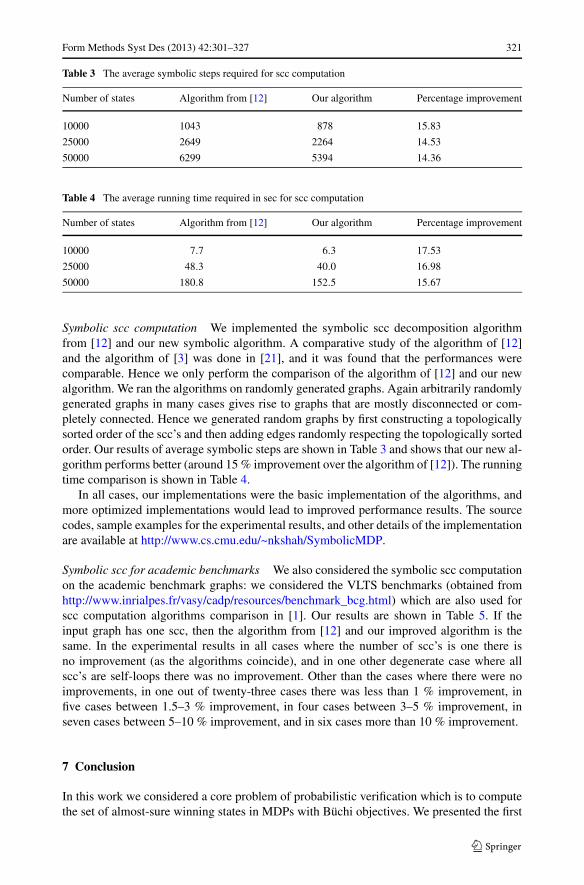
Table 3 The average symbolic steps required for scc computation

Number of states Algorithm from [12] Our algorithm Percentage improvement

10000 1043 878 15.83

25000 2649 2264 14.53

50000 6299 5394 14.36

Table 4 The average running time required in sec for scc computation

Number of states Algorithm from [12] Our algorithm Percentage improvement

10000 7.7 6.3 17.53

25000 48.3 40.0 16.98

50000 180.8 152.5 15.67

Symbolic scc computation We implemented the symbolic scc decomposition algorithmfrom [12] and our new symbolic algorithm. A comparative study of the algorithm of [12]and the algorithm of [3] was done in [21], and it was found that the performances werecomparable. Hence we only perform the comparison of the algorithm of [12] and our newalgorithm. We ran the algorithms on randomly generated graphs. Again arbitrarily randomlygenerated graphs in many cases gives rise to graphs that are mostly disconnected or com-pletely connected. Hence we generated random graphs by first constructing a topologicallysorted order of the scc’s and then adding edges randomly respecting the topologically sortedorder. Our results of average symbolic steps are shown in Table 3 and shows that our new al-gorithm performs better (around 15 % improvement over the algorithm of [12]). The runningtime comparison is shown in Table 4.

In all cases, our implementations were the basic implementation of the algorithms, andmore optimized implementations would lead to improved performance results. The sourcecodes, sample examples for the experimental results, and other details of the implementationare available at http://www.cs.cmu.edu/~nkshah/SymbolicMDP.

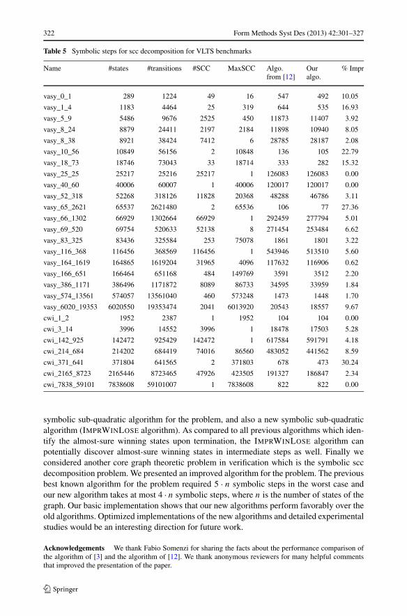
Symbolic scc for academic benchmarks We also considered the symbolic scc computationon the academic benchmark graphs: we considered the VLTS benchmarks (obtained fromhttp://www.inrialpes.fr/vasy/cadp/resources/benchmark_bcg.html) which are also used forscc computation algorithms comparison in [1]. Our results are shown in Table 5. If theinput graph has one scc, then the algorithm from [12] and our improved algorithm is thesame. In the experimental results in all cases where the number of scc’s is one there isno improvement (as the algorithms coincide), and in one other degenerate case where allscc’s are self-loops there was no improvement. Other than the cases where there were noimprovements, in one out of twenty-three cases there was less than 1 % improvement, infive cases between 1.5–3 % improvement, in four cases between 3–5 % improvement, inseven cases between 5–10 % improvement, and in six cases more than 10 % improvement.

7 Conclusion

In this work we considered a core problem of probabilistic verification which is to computethe set of almost-sure winning states in MDPs with Büchi objectives. We presented the first

http://www.cs.cmu.edu/~nkshah/SymbolicMDP

http://www.inrialpes.fr/vasy/cadp/resources/benchmark_bcg.html


Table 5 Symbolic steps for scc decomposition for VLTS benchmarks

Name #states #transitions #SCC MaxSCC Algo.from [12]

Ouralgo.

% Impr

vasy_0_1 289 1224 49 16 547 492 10.05

vasy_1_4 1183 4464 25 319 644 535 16.93

vasy_5_9 5486 9676 2525 450 11873 11407 3.92

vasy_8_24 8879 24411 2197 2184 11898 10940 8.05

vasy_8_38 8921 38424 7412 6 28785 28187 2.08

vasy_10_56 10849 56156 2 10848 136 105 22.79

vasy_18_73 18746 73043 33 18714 333 282 15.32

vasy_25_25 25217 25216 25217 1 126083 126083 0.00

vasy_40_60 40006 60007 1 40006 120017 120017 0.00

vasy_52_318 52268 318126 11828 20368 48288 46786 3.11

vasy_65_2621 65537 2621480 2 65536 106 77 27.36

vasy_66_1302 66929 1302664 66929 1 292459 277794 5.01

vasy_69_520 69754 520633 52138 8 271454 253484 6.62

vasy_83_325 83436 325584 253 75078 1861 1801 3.22

vasy_116_368 116456 368569 116456 1 543946 513510 5.60

vasy_164_1619 164865 1619204 31965 4096 117632 116906 0.62

vasy_166_651 166464 651168 484 149769 3591 3512 2.20

vasy_386_1171 386496 1171872 8089 86733 34595 33959 1.84

vasy_574_13561 574057 13561040 460 573248 1473 1448 1.70

vasy_6020_19353 6020550 19353474 2041 6013920 20543 18557 9.67

cwi_1_2 1952 2387 1 1952 104 104 0.00

cwi_3_14 3996 14552 3996 1 18478 17503 5.28

cwi_142_925 142472 925429 142472 1 617584 591791 4.18

cwi_214_684 214202 684419 74016 86560 483052 441562 8.59

cwi_371_641 371804 641565 2 371803 678 473 30.24

cwi_2165_8723 2165446 8723465 47926 423505 191327 186847 2.34

cwi_7838_59101 7838608 59101007 1 7838608 822 822 0.00

symbolic sub-quadratic algorithm for the problem, and also a new symbolic sub-quadraticalgorithm (IMPRWINLOSE algorithm). As compared to all previous algorithms which iden-tify the almost-sure winning states upon termination, the IMPRWINLOSE algorithm canpotentially discover almost-sure winning states in intermediate steps as well. Finally weconsidered another core graph theoretic problem in verification which is the symbolic sccdecomposition problem. We presented an improved algorithm for the problem. The previousbest known algorithm for the problem required 5 · n symbolic steps in the worst case andour new algorithm takes at most 4 · n symbolic steps, where n is the number of states of thegraph. Our basic implementation shows that our new algorithms perform favorably over theold algorithms. Optimized implementations of the new algorithms and detailed experimentalstudies would be an interesting direction for future work.

Acknowledgements We thank Fabio Somenzi for sharing the facts about the performance comparison ofthe algorithm of [3] and the algorithm of [12]. We thank anonymous reviewers for many helpful commentsthat improved the presentation of the paper.


Appendix

8.1 Technical details of improved symbolic scc algorithm

The pseudocode of SCCFIND is formally given as Algorithm 4. The correctness analy-sis and the analysis of the number of symbolic steps is given in [12]. The pseudocode ofIMPROVEDSCCFIND is formally given as Algorithm 5. The main changes of IMPROVED-SCCFIND from SCCFIND are as follows: (1) instead of SKELFWD the algorithm IM-PROVEDSCCFIND calls procedure IMPROVEDSKELFWD that returns an additional set P

and IMPROVEDSKELFWD is invoked with an additional argument that is U ; (2) in line 4 ofIMPROVEDSCCFIND the set SCC is initialized to P instead of s. The main difference ofIMPROVEDSKELFWD from SKELFWD is as follows: (1) the set P is computed in line 4 ofIMPROVEDSKELFWD as FWSet ∩ Q, where Q is the set passed by IMPROVEDSCCFIND

as the argument; and (2) in the while loop it is checked if the element popped intersects withP and if yes, then the procedure breaks the while loop. The correctness argument from thecorrectness of SCCFIND is already shown in Sect. 5.1.

Symbolic steps analysis We now present the detailed symbolic steps analysis of the algo-rithm. As noted in Sect. 3.2, common symbolic operations on a set of states are Pre, Postand CPre. We note that these operations involve symbolic sets of 2 · log(n) variables, ascompared to symbolic sets of log(n) variables required for operations such as union, inter-section and set difference. Thus only Pre, Post and CPre are counted as symbolic steps, asdone in [12]. The total number of other symbolic operations is also O(|S|). We note thatonly lines 5 and 10 of IMPROVEDSCCFIND and lines 3.3 and 7.3 of IMPROVEDSKELFWD

involve Pre and Post operations.In the following, we charge the costs of these lines to states in order to achieve the

3 · |S| + N(G) bound for symbolic steps. We define subspine-set as NewSet returned byIMPROVEDSKELFWD and show the following result.

Lemma 4 For any spine-set U and its end vertex u, T is a subspine-set iff U \T ⊆ SCC(u).

Proof Note that while constructing a subspine-set T , we stop the construction when wefind any state v ∈ FWSet ∩ U from the spine set. Now clearly since v ∈ U , there is a pathfrom v to u. Also, since we found this state in FW(u), there is a path from u to v. Hence,v ∈ SCC(u). Also, each state that we are omitting by stopping construction of T has theproperty that there is a path from u to that state and a path from that state to v. This impliesthat all the states we are omitting in construction of T are in SCC(u). �

Note that since we pass NewSet \ SCC in the subsequent call to IMPROVEDSCCFIND,it will actually be a spine set for the reduced problem. In the following lemma we show thatany state can be part of subspine-set at most once, as compared to twice in the SCCFIND

procedure in [12]. This lemma is one of the key points that lead to the improved analysis ofsymbolic steps required.

Lemma 5 Any state v can be part of subspine-set at most once.

Proof In [12], the authors show that any state v can be included in spine sets at most twicein SKELFWD. The second time the state v is included is in line 6 of SKELFWD when theSCC(v) of the state is to be found. In contrast, IMPROVEDSKELFWD checks intersection of


Algorithm 4 SCCFIND

Input: (S,E, 〈U, s〉), i.e., a graph (S,E) with spine set (U, s).Output: SCCPartition i.e. the set of SCCs of the graph (S,E)

Initialize SCCPartition := ∅; FWSet := ∅;1. if (S = ∅) then

1.1 return;2. if (U = ∅) then

2.1 s := pick(S)

3. 〈FWSet,NewSet,NewState〉 := SKELFWD(S,E, s)

4. SCC = s

5. while (((Pre(SCC) ∩ FWSet) \ SCC) �= ∅) do5.1 SCC := SCC ∪ (Pre(SCC) ∩ FWSet)

6. SCCPartition := SCCPartition ∪ {SCC}(Recursive call on S \ FWSet)

7. S′ := S \ FWSet8. E′ := E ∩ (S′ × S′)9. U ′ := U \ SCC10. s′ := Pre(SCC ∩ U) ∩ (S \ SCC)

11. SCCPartition := SCCPartition ∪ SCCFIND(S′,E′, 〈U ′, s′〉)(Recursive call on FWSet \ SCC)

12. S′ := FWSet \ SCC13. E′ := E ∩ (S′ × S′)14. U ′ := NewSet \ SCC15. s′ := NewState \ SCC16. SCCPartition := SCCPartition ∪ SCCFIND(S′,E′, 〈U ′, s′〉)17. Return SCCPartition

Procedure SKELFWD

Input: (S,E, s), i.e., a graph (S,E) with a state s ∈ S.Output: 〈FWSet,NewSet,NewState〉,

i.e. forward set FWSet, new spine-set NewSet and NewState ∈ NewSet1. Let stack be an empty stack of sets of nodes2. L := s

3. while (L �= ∅) do3.1 Push(stack,L)

3.2 FWSet := FWSet ∪ L

3.3 L := Post(L) \ FWSet4. L := Pop(stack)5. NewSet := NewState := pick(L)

6. while (stack �= ∅) do6.1 L := Pop(stack)6.2 NewSet := NewSet ∪ pick(Pre(NewSet) ∩ L)

7. return 〈FWSet,NewSet,NewState〉

the subspine-set being constructed with the set P that contains the states of SCC(v) whichare already in a subspine-set. When this happens, it stops the construction of the subspine-set. Now if v is already included in the subspine-set, then it will be part of P and would notbe included in subspine-set again. Hence, v can be part of subspine-set at most once. �

Lemma 6 States added in SCC by iteration of line 5 of IMPROVEDSCCFIND are exactlythe states which are not part of any subspine-set.

Proof We see that in line 5 of IMPROVEDSCCFIND, we start from SCC = P and then wefind the SCC by backward search. Also, P has all the states from SCC which are part ofany subspine-set. Hence, the extra states that are added in SCC are states which are neverincluded in a subspine-set. �


Algorithm 5 IMPROVEDSCCFIND

Input: (S,E, 〈U, s〉), i.e., a graph (S,E) with spine set (U, s).Output: SCCPartition, the set of SCCs of the graph (S,E)

Initialize SCCPartition := ∅; FWSet := ∅;1. if (S = ∅) then

1.1 return;2. if (U = ∅) then

2.1 s := pick(S)

3. 〈FWSet,NewSet,NewState,P 〉 := IMPROVEDSKELFWD(S,E,U, s)

4. SCC = P

5. while (((Pre(SCC) ∩ FWSet) \ SCC) �= ∅) do5.1 SCC := SCC ∪ (Pre(SCC) ∩ FWSet)

6. SCCPartition := SCCPartition ∪ {SCC}(Recursive call on S \ FWSet)

7. S′ := S \ FWSet8. E′ := E ∩ (S′ × S′)9. U ′ := U \ SCC10. s′ := Pre(SCC ∩ U) ∩ (S \ SCC)

11. SCCPartition := SCCPartition ∪ IMPROVEDSCCFIND(S′,E′, 〈U ′, s′〉)(Recursive call on FWSet \ SCC)

12. S′ := FWSet \ SCC13. E′ := E ∩ (S′ × S′)14. U ′ := NewSet \ SCC15. s′ := NewState \ SCC16. SCCPartition := SCCPartition ∪ IMPROVEDSCCFIND(S′,E′, 〈U ′, s′〉)

Procedure IMPROVEDSKELFWD

Input: (S,E,Q, s), i.e., a graph (S,E) with a set Q and a state s ∈ S.Output: 〈FWSet,NewSet,NewState,P 〉1. Let stack be an empty stack of sets of nodes2. L := s

3. while (L �= ∅) do3.1 Push(stack,L)

3.2 FWSet := FWSet ∪ L

3.3 L := Post(L) \ FWSet4. P := FWSet ∩ Q

5. L := Pop(stack)6. NewSet := NewState := pick(L)

7. while (stack �= ∅) do7.1 L := Pop(stack)7.2 if (L ∩ P �= ∅) then

7.2.1 break while loop7.3 else NewSet := NewSet ∪ pick(Pre(NewSet) ∩ L)

8. return 〈FWSet,NewSet,NewState,P 〉

Charging symbolic steps to states We now consider three cases to charge symbolic stepsto states and scc’s.

1. Charging states included in subspine-set. First, we see that the number of times the loopof line 3 in IMPROVEDSKELFWD is executed is equal to the size of the spine set thatSKELFWD would have computed. Using Lemma 4, we can charge one symbolic step toeach state of the subspine-set and each state of the SCC that is being computed. Now, thenumber of times line 7.3 of IMPROVEDSKELFWD is executed equals the size of subspine-set that is computed. Hence, we charge one symbolic step to each state of subspine-setfor this line.Now we summarize the symbolic steps charged to each state which is part of somesubspine-set. First time when a state gets into a subspine-set, it is charged two steps,


one for line 3.3 and one for line 7.3 of IMPROVEDSKELFWD. If its SCC is not foundin the same call to IMPROVEDSCCFIND, then it comes into action once again when itsSCC is being found. By Lemma 5, it is never again included in a subspine set. Hence inthis call to IMPROVEDSKELFWD, it is only charged one symbolic step for line 3.3 andnone for line 7.3 as line 7.3 is charged to states that become part of the newly constructedsubspine-set. Also because of Lemma 6, since this state is in a subspine-set, it is notcharged anything for line 5 of IMPROVEDSCCFIND. Hence, a state that occurs in anysubspine-set is charged at most three symbolic steps.

2. Charging states not included in subspine-set. For line 5 of IMPROVEDSCCFIND, thenumber of times it is executed is the number of states that are added to SCC after initial-ization to SCC = P . Using Lemma 6, we charge one symbolic step to each state of thisSCC that is never a part of any subspine-set. Also, we might have charged one symbolicstep to such a state for line 3.3 of IMPROVEDSKELFWD when we called it. Hence, eachsuch state is charged at most two symbolic steps.

3. Charging SCCs. For line 10 of IMPROVEDSCCFIND, we see that it is executed onlyonce in a call to IMPROVEDSCCFIND that computes a SCC. Hence, the total numberof times line 10 is executed equals N(G), the number of SCCs of the graph. Hence, wecharge each SCC one symbolic step for this line.

The above argument shows that the number of symbolic steps that the algorithm IMPROVED-SCCFIND requires is at most 3 · |S|+N(G). This completes the formal proof of Theorem 8.

We now present an example that presents a family of graphs with k · n states, where theSCCFIND algorithm takes almost 5 ·k ·n symbolic steps, whereas the IMPROVEDSCCFIND

algorithm takes at most 3 · k · n + n symbolic steps.

Example 1 Let k,n ∈ N. Consider a graph with k ·n states such that the states are numberedfrom 1 to k · n. The edges are as follows: (1) for all states 1 ≤ i ≤ k · n − 1, there is an edge(i, i + 1) (i.e., the states are all in a line); and (2) for all 1 ≤ i ≤ n, there is an edge fromstate k · i to state (i − 1) · k + 1. We will show that the SCCFIND algorithm requires roughly(5 · k − 1) · n symbolic steps on this graph. Note the number of scc’s in this graph is n, andhence by Theorem 8 the IMPROVEDSCCFIND algorithm takes at most 3 · k ·n+n symbolicsteps.

We now analyze the symbolic steps required by the SCCFIND algorithm, and our analy-sis is in two steps.

1. Step 1. In the beginning, starting from the state 1 of the graph, the algorithm performs aforward and backward search to find the spine set. This will have a cost of two symbolicsteps per state (one symbolic step while going forward, and one symbolic step whilegoing backward), except for the first vertex which gets charged only one symbolic step(it does not get charged while going backwards). This gives a cost of 2 ·k ·n−1 symbolicsteps. After this, the first scc will be found with an additional cost of only k, and the firstdiscovered scc consists of states {1,2, . . . , k}. Hence the total symbolic steps required is2 · k · n − 1 + k.

2. Step 2. After Step 1, the algorithm will start finding scc’s from the end of the spine set.So consider the set of last k states from k · (n−1)+1 to n ·k. The algorithm will pick thelast state n ·k, find a spine set, consisting of the last k states (states k · (n−1)+1 to n ·k).This will have a cost of 2 · k − 1 symbolic steps (k symbolic steps for the forward search,and k − 1 symbolic steps for the backward search). After this, the algorithm will findthe scc containing the last state n · k (i.e., the scc that consists of states {k · (n − 1) + 1,

k · (n − 1) + 2, . . . , n · k}), and this takes k symbolic steps as there are k vertices in the


scc. Now Step 2 is repeated with state k · (n − 1), and then repeated for state k · (n − 2)

and so on. So the cost for every scc, except the very first one, is 2k − 1 + k = 3k − 1.Since there are n scc’s, the total number of symbolic steps required for Step 2 is at least(3 · k − 1) · (n − 1).

Hence the total symbolic steps required for the algorithm is at least

2 · k · n − 1 + k + (3 · k − 1) · (n − 1) = (5 · k − 1) · n − 2 · k.

Note that with k = n, SCCFIND takes at least 5 · n2 − 3 · n symbolic steps, whereas theIMPROVEDSCCFIND takes at most 3 · n2 + n symbolic steps.

References

1. Barnat J, Chaloupka J, van de Pol J (2011) Distributed algorithms for SCC decomposition. J Log Comput21(1):23–44

2. Bianco A, de Alfaro L (1995) Model checking of probabilistic and nondeterministic systems. In:FSTTCS 95. LNCS, vol 1026. Springer, Berlin, pp 499–513

3. Bloem R, Gabow HN, Somenzi F (2000) An algorithm for strongly connected component analysis in logsymbolic steps. In: FMCAD, pp 37–54

4. Chatterjee K, Henzinger M (2011) Faster and dynamic algorithms for maximal end-component decom-position and related graph problems in probabilistic verification. In: SODA, pp 1318–1336

5. Chatterjee K, Jurdzinski M, Henzinger TA (2003) Simple stochastic parity games. In: CSL’03. LNCS,vol 2803. Springer, Berlin, pp 100–113

6. Chatterjee K, Jurdzinski M, Henzinger TA (2004) Quantitative stochastic parity games. In: SODA’04.SIAM, Philadelphia, pp 121–130

7. Courcoubetis C, Yannakakis M (1995) The complexity of probabilistic verification. J ACM 42(4):857–907

8. de Alfaro L (1997) Formal verification of probabilistic systems. PhD thesis, Stanford University9. de Alfaro L, Faella M, Majumdar R, Raman V (2005) Code-aware resource management. In: EM-

SOFT 05. ACM, New York10. de Alfaro L, Roy P (2007) Magnifying-lens abstraction for Markov decision processes. In: CAV, pp 325–

33811. Filar J, Vrieze K (1997) Competitive Markov decision processes. Springer, Berlin12. Gentilini R, Piazza C, Policriti A (2003) Computing strongly connected components in a linear number

of symbolic steps. In: SODA, pp 573–58213. Howard H (1960) Dynamic programming and Markov processes. MIT Press, Cambridge14. Immerman N (1981) Number of quantifiers is better than number of tape cells. J Comput Syst Sci

22:384–40615. Kemeny JG, Snell JL, Knapp AW (1966) Denumerable Markov chains. Van Nostrand, Princeton16. Kwiatkowska M, Norman G, Parker D (2000) Verifying randomized distributed algorithms with prism.

In: Workshop on advances in verification (WAVE’00)17. Pogosyants A, Segala R, Lynch N (2000) Verification of the randomized consensus algorithm of Aspnes

and Herlihy: a case study. Distrib Comput 13(3):155–18618. Puterman ML (1994) Markov decision processes. Wiley, New York19. Segala R (1995) Modeling and verification of randomized distributed real-time systems. PhD thesis, MIT

Technical Report MIT/LCS/TR-67620. Sleator DD, Tarjan RE (1983) A data structure for dynamic trees. J Comput Syst Sci 26(3):362–39121. Somenzi F. Personal communication22. Somenzi F (1998) Colorado university decision diagram package. http://vlsi.colorado.edu/pub/23. Stoelinga MIA (2002) Fun with FireWire: experiments with verifying the IEEE1394 root contention

protocol. In: Formal aspects of computing24. Thomas W (1997) Languages, automata, and logic. In: Rozenberg G, Salomaa A (eds) Beyond words.

Handbook of formal languages, vol 3. Springer, Berlin, pp 389–455. Chap 7

http://vlsi.colorado.edu/pub/

symbolic algorithms for qualitative analysis of …nisarg/papers/symbolicmdp.fmsd.pdfform methods...

Documents