symbol timing and coarse classification of phase · pdf filethe system is constructed to run...

Symbol Timing and Coarse Classification of Phase Modulated

Signals on a Standalone SDR Platform

Gladstone Marballie

Thesis submitted to the faculty of the Virginia Polytechnic Institute and State University

in partial fulfillment of the requirements for the degree of

Master of Science

In

Electrical Engineering

Dr. Charles W. Bostian

Dr. Tim Pratt

Dr. Cameron Patterson

October 6, 2010

Blacksburg, Virginia

Keywords: Cognitive Radio, SDR, Symbol Timing, Signal Classification, FPGA, DSP

Copyright 2010, Gladstone Marballie

Symbol Timing and Coarse Classification of Phase Modulated

Signals on a Standalone SDR Platform

Gladstone Marballie

ABSTRACT

The Universal Classifier Synchronizer (UCS) is a Cognitive Radio system/sensor that can

detect, classify, and extract the relevant parameters from a received signal to establish

physical layer communications using the received signal’s profile. The current

implementation is able to identify signals including AM, FM, MPSK, QAM, MFSK, and

OFDM. The system is constructed to run on a Universal Software Radio Peripheral

(USRP) with the GNU Radio software toolkit and also runs on an Anritsu™ signal

analyzer. In both prototypes, the UCS system runs on a host computer’s General Purpose

Processor (GPP) and is constructed in Matlab™. The aim is to then create a portable and

standalone version of the UCS system as an intermediate step towards building a future

commercial implementation. This application and particular implementation aims to run

on a Lyrtech SFF SDR platform and uses its FPGA and DSP modules for

implementation. This platform is one of the more advanced SDR platforms available, and

the aim is to develop parts of the UCS system to run on this platform. The aim is to

eventually develop the complete UCS cognitive radio system on the Lyrtech SFF SDR

platform that can act as a standalone portable cognitive radio system. The modules

created and implanted/implemented on the SDR hardware are the Bandwidth Estimation,

and Symbol Timing & Coarse Classification modules. This is the system decision path

towards classification, synchronization, and demodulation of digital phase modulated

signals (QAM and MPSK signal types) and also analog signals. The Digital Receiver

Module (DRM) is implemented on the FPGA and takes care of all the digital down

conversions, mixing, decimation, and low pass filtering. The FPGA is connected to the

DSP module via a bus subsystem where the DSP receives real-time base-band complex

IQ samples for further signal processing. The main UCS algorithm runs on the platform’s

DSP and is compiled from executable embedded C-code. Therefore, this system can then

be implemented on virtually any setup that has an RF front end, digital receiver module,

and processing module that will execute floating and fixed point C-code with minor

changes.

iii

Acknowledgments

I would like to thank Dr. Charles Bostian for his motivation and encouragement to take

on the journey of graduate school. I would also like thank him for providing the

opportunity to become a part of CWT where I have learned Software Defined and

Cognitive Radio. I want to thank him for his continued support over the years.

I would also like to thank Dr. Tim Pratt and Dr. Cameron Patterson for being a part of my

committee.

I would like to thank all the committee members for providing great classroom

instruction over the years. I could not have asked for better instructors and more

interesting lectures. I give credit to Dr. Bostian for his enthralling classroom lectures on

AC Circuits and Radio Engineering. I give credit to Dr. Patterson for his thorough

instruction on Microcontrollers and FPGAs. I give credit to Dr. Pratt for his many

remarkable lectures on Communication Systems Design, Satellite Communications, and

Radar Systems.

I would like to thank all my fellow graduate students during my time at CWT for making

graduate school a memorable experience. I enjoyed the opportunity to interact with

everyone and learn about the different cultural backgrounds. I would also like to thank

Ms. Judy Hood for taking very good care of all the CWT students over the years. Her

support has made all things at CWT run smoothly over the years.

Finally, I would like to thank my family and friends for their love and support over the

years.

iv

Grant Information

This project is supported by Awards 2005-IJ-CX-K017 and 2009-SQ-B9-K011 awarded

by the National Institute of Justice, Office of Justice Programs, US Department of Justice.

The opinions, findings, and conclusions or recommendations expressed are those of the

author and do not necessarily reflect the views of the Department of Justice.

This material is based upon work supported by the National Science Foundation under

Grant No. CNS-0519959. Any opinions, findings, and conclusions or recommendations

expressed in this material are those of the author(s) and do not necessarily reflect the

views of the National Science Foundation (NSF).

v

Table of Contents

Acknowledgments ............................................................................................................ iii

Grant Information ........................................................................................................... iv

List of Figures .................................................................................................................. vii

List of Acronyms .............................................................................................................. ix

Chapter 1: Introduction ....................................................................................................1

1.1 Motivation and Objectives .........................................................................................1

1.2 Thesis Outline .........................................................................................................2

Chapter 2: System Description and Current Literature ................................................4

2.1 System Overview .......................................................................................................4

2.2 Review of Current Literature ..................................................................................6

Chapter 3: Digital Signal Bandwidth Estimation ...........................................................8

3.1 Introduction ................................................................................................................8

3.2 Histogram of PSD Technique .................................................................................8

3.3 Module Implementation .............................................................................................9

3.31 Simple Histogram of the PSD ..............................................................................9

3.32 Noise Isolation of the Histogram Distribution .....................................................9

3.4 Conclusion ................................................................................................................11

Chapter 4: Symbol Timing ..............................................................................................12

4.1 Introduction and Overview of Symbol Timing ........................................................12

4.2 Vector Re-sampling ..................................................................................................14

4.21 Overview ............................................................................................................14

4.22 Combined Interpolation and Decimation for Re-sampling ................................20

4.23 Finite Impulse Response Filter Design...............................................................20

4.24 Re-sampling Filter Design in C ..........................................................................24

4.25 Convolution in C ................................................................................................29

4.26 Symbol Timing Use of Re-sampling ..................................................................30

4.27 Re-sample Example and Plots for Symbol Timing ............................................32

vi

4.3 Symbol Rate Estimation and Coarse Classification .................................................35

4.4 Reshaping and Variance Among Samples ...............................................................36

4.5 Symbol Timing Conclusion .....................................................................................40

Chapter 5: FPGA Digital Receiver and SDR Platform ................................................41

5.1 SDR Platform Overview ..........................................................................................41

5.2 Digital Receiver Overview and FPGA Implementation ..........................................42

5.3 Conclusion ................................................................................................................50

Chapter 6: Conclusion and Future Work ......................................................................51

6.1 Summary and Conclusion ........................................................................................51

6.2 Future Work .............................................................................................................51

References .........................................................................................................................54

Appendix A: Source Code Listing for Bandwidth Estimation ....................................56

Appendix B: Source Code Listing for Symbol Timing Estimation .............................65

vii

List of Figures

Figure 1.1: Overview of Thesis and Implementation ..........................................................3

Figure 2.1: Complete System Diagram ................................................................................4

Figure 3.1: PSD of a QPSK Signal ......................................................................................8

Figure 3.2: Histogram of PSD for DQPSK ..........................................................................9

Figure 3.3: Histogram Distribution and Noise Isolation Plot ............................................10

Figure 4.1: Illustration of Symbol Timing and Samples per Symbol ................................13

Figure 4.2: Plot of example Samples_Vector .....................................................................15

Figure 4.3: Alternate Plot of Samples_Vector as a Stem ...................................................16

Figure 4.4: Plot of Up-sampled Samples_Vector as a Linear Plot .....................................16

Figure 4.5: Up-sampled Samples_Vector as a Stem Plot ...................................................17

Figure 4.6: Plot of example Samples_Vector Up-sampled and Filtered (Interpolated) .....17

Figure 4.7: Alternate view of Interpolated Samples_Vector as a Stem Plot .....................18

Figure 4.8: Interpolated Samples_Vector Decimated by a Factor of 9 ..............................19

Figure 4.9: Alternate View of Decimated Vector as a Stem ..............................................19

Figure 4.10: FIR Low-Pass Filter for Re-sampling ...........................................................20

Figure 4.11: Plot of ideal Sinc Pulse ..................................................................................21

Figure 4.12: Example Truncated Right Shifted Sinc Pulse ...............................................22

Figure 4.13: Plot of a Blackman Window .........................................................................22

Figure 4.14: Windowed-Sinc FIR filter via Blackman Window .......................................24

Figure 4.15: Snapshot of C – code Initializations of FIR vectors .....................................25

Figure 4.16: Code snapshot of Truncated and shifted Filter Kernel and Blackman

Window Calculation ..........................................................................................................26

Figure 4.17: Code Composer Studio C-Simulated Plot of Filter_Kernel and

BlackMan_Window from data memory .............................................................................26

Figure 4.18: Windowed_Filter Kernel Plot with 501 Taps in Code Composer Studio .....27

Figure 4.19: C-Code snapshot showing the Normalization of Filter Kernel for Unity Gain

............................................................................................................................................28

viii

Figure 4.20: Normalized Filter Kernel with Unity Gain ....................................................28

Figure 4.21: Convolution of Filter with Ups-sampled Data ..............................................29

Figure 4.22: Code Snapshot of C-Code Implementation of Convolution Sum .................30

Figure 4.23: Resampling Code Snapshot ...........................................................................32

Figure 4.24: Plot of Real of IQ samples and Re-sampled Real IQ samples in Matlab

Simulation ..........................................................................................................................33

Figure 4.25: Plots of Real Parts of Constellation and Re-sampled Constellation with delay

............................................................................................................................................34

Figure 4.26: Real of Re-sampled IQ with Delay Compensation .......................................35

Figure 4.27: Reshaped Absolute Value of Constellation ...................................................37

Figure 4.28: Row by Row Variance from Reshaped Constellation ...................................37

Figure 4.29: Reshaped Data in Original Format Row-Major ............................................37

Figure 5.1: Lyterch SFF SDR Platform .............................................................................42

Figure 5.2: Super-het Receiver Block Diagram .................................................................43

Figure 5.3: Digital Receiver Block Diagram .....................................................................44

Figure 5.3: Digital Receiver Block Diagram .....................................................................44

Figure 5.4: Isolated Digital Receiver Blocks .....................................................................45

Figure 5.5: FPGA Digital Receiver Implementation .........................................................46

Figure 5.6: Digital Local Oscillator Configuration ............................................................47

Figure 5.7: Encapsulated DRM with view of Digital Filter

............................................................................................................................................48

Figure 5.8: : FIR Filter Configuration................................................................................48

Figure 5.9: Encapsulated Digital Reciever Module and Synthesis Configuration ............49

Figure 5.10: FPGA Device Utilization ..............................................................................50

ix

List of Acronyms

ADC Analog to Digital Converter

AM Amplitude Modulation

BW Bandwidth

CCC Common Control Channel

CWT Center for Wireless Telecommunications

CR Cognitive Radio

DAC Digital to Analog Converter

DBPSK Differential Binary Phase Shift Keying

DDC Digital Down Converter

DDS Direct Digital Synthesizer

DRM Digital Receiver Module

DSA Dynamic Spectrum Access

DSP Digital Signal Processor (or Processing)

FFT Fast Fourier Transform

FPGA Field Programmable Gate Array

FM Frequency Modulation

GPP General Purpose Processor

IF Intermediate Frequency

OFDM Orthogonal Frequency Division Multiplexing

OSA Opportunistic Spectrum Access

OTA Over The Air

MDBK Model Based Design Kit

ML Maximum Likelihood

PLL Phase Lock Loop

PSD Power Spectral Density

QAM Quadrature Amplitude Modulation

QPSK Quadrature Phase Shift Keying

16QAM 16 Quadrature Amplitude Modulation

RF Radio Frequency

SDR Software Defined Radio

SFF Small Form Factor

SNR Signal to Noise Ratio

SIGINT Signal Intelligence

SUPER-HET Super Heterodyne

UCS Universal Classification Synchronization

VHDL VHSIC Hardware Description Language

VHSIC Very-High-Speed Integrated Circuit

1

Chapter 1: Introduction

1.1 Motivation and Objectives

Software Defined Radio (SDR) has become one of the more popular areas of research in

communication systems and electrical engineering. Although in its infancy, this new concept is

seeing its application to many areas such as military and commercial. The concept behind SDR is

implementing radio components in software on a processor, components which were typically

implemented in physical hardware. Cognitive Radio (CR) technology is a phenomenon that is

built on top of the evolution of SDR and is essentially an intelligent SDR. A CR is a radio that is

aware of its surroundings and can adapt based on predefined objectives. In this paper, we

introduce the development and implementation of a CR sensor designed for the use in embedded

applications. Presented here however is not a full CR system itself, but the modules described

play a major role in a much bigger CR system and can help make decisions on the operating

conditions of the communicating environment. Universal Classifier Synchronizer (UCS) is a CR

sensor that can detect, classify, and extract all of the parameters from a received signal to

establish physical layer communications using the received signal’s profile. At the heart of the

UCS system lies the symbol timer, which is used to determine the symbol rate and bit rate that is

used in the communicating signal and is the major topic of this paper. A CR system with a “UCS

engine” on board has the power to detect, receive, classify, demodulate and reconfigure itself to

communicate, without any prior knowledge of the communicating environment [Chen, 2008].

In today’s world, the wireless spectrum is shared by innumerable applications ranging from

cellular telephone networks to television transmission, and from consumer radios to military

communication systems, to name a few. Under these circumstances there is a constant “spectrum

war” between various users and policy makers regarding spectrum allocation. Use of CR and

dynamic spectrum sensing, wherein no user or application is permanently assigned a particular

frequency band, seems to be a very good solution for more efficient use of available wireless

spectrum. Dynamic Spectrum Access (DSA) technology is developing to provide intelligent

schemes that use spectrum during times when other users or primary users are not operating.

Whether centralized or distributed, spectrum sharing techniques in DSA require the use of a

Common Control Channel (CCC) to accommodate spectrum sharing. The CCC will facilitate

functionalities such as handshaking between CR nodes, communicating with a central entity or

sharing spectrum information across the network. However, due to the fact that DSA CR nodes

share spectrum opportunistically, a fixed CCC is not possible in most networks. Therefore, a

DSA CR with a UCS engine has the ability to operate free of a CCC as it senses and

interoperates with received signals without predefined information from the transmitter. It also

provides better spectrum sensing, as it is aware of other signals communicating in nearby

channels and has increased perception of the interference caused by these signals. This enables

the DSA CR it to make better decisions on channels used to communicate and can switch if

needed.

2

1.2 Thesis Outline

In this thesis, Bandwidth Estimation and Symbol Timing modules are created and implemented

for the use on portable embedded Cognitive and Software Defined Radio hardware. The overall

idea behind this work is to create portable parts of the Virginia Tech Universal Signal Classifier

(UCS) that is already implemented on computers running Matlab™ code for use on embedded

Cognitive SDRs. This work also aims to prove that the new concept of embedded Cognitive SDR

can be used across many different RF platforms and boards for various applications. This

application and particular implementation aims to run on a Lyrtech SFF SDR platform and uses

its FPGA and DSP modules for implementation. This platform is one of the more advanced SDR

platforms available and the aim is develop parts of the UCS system to run on this platform. The

Digital Receiver Module (DRM) is implemented on the FPGA and takes care of all the digital

down conversions, mixing, decimation, and low pass filtering. The FPGA is connected to the

DSP module via a bus subsystem where the DSP receives real-time base-band Complex IQ

samples for further signal processing. The main Signal Detection and Classification Algorithm

runs on the platform’s DSP and is compiled from executable embedded C-code. Therefore, this

system can then be implemented on virtually any setup that has a RF front end, digital receiver

module, and processing module that will execute floating and fixed point C-code. The

deliverable of this thesis is portable C-code implementations of various parts of this UCS system

that performs its functionality when mapped to different SDR hardware, in this case specifically

a Lyrtech SFF SDR platform’s DSP. Despite being one of the more modern standalone SDR

platforms, the Lyrtech SFF SDR platform is also known across the SDR community to be

difficult to work with. Therefore, implementing parts of a CR system as is described on this

platform is also an important contribution and milestone in SDR community.

The important parts of this research and my major contributions are implementations of:

1) Bandwidth Estimation of radio signals using the histogram method of power spectral density,

2) Symbol Timing module for Coarse Classification of potential digital phase modulated signals, and

3) FPGA Digital Receiver Module created for the Lyrtech SFF SDR Platform.

Chapter 3 introduces the Bandwidth Estimation technique used in the system as it exists in

Matlab™ and outlines the major functionalities and concepts behind this module. This chapter

also discusses the C-code implementation in detail along with the final testing results in

simulation from captured samples. Chapter 4 introduces the Symbol Timing concept as it exists

in Matlab™ and outlines the functionalities. This chapter also provides the C-code translation

and implementation of this module and detailed work of each submodule that is used in the

implementation. The final section of this chapter verifies the module, including testing results of

captured samples for simulation. Chapter 5 first provides a brief introduction to the hardware

platform used for implementation, the Lyrtech SFF SDR platform. This chapter also describes

the creation of the DRM implemented on the FPGA. Chapter 6 provides the concluding remarks

of the report and talks about the future work that will be needed to complete the next phase of the

system. The documented source codes are provided as an appendix.

The figure 1.1 below provides an overview of this thesis and implementation.

3

Figure 1.1: Overview of Thesis and Implementation

4

Chapter 2: System Description and Current

Literature

2.1 System Overview

As introduced previously, the Universal Classifier Synchronizer (UCS) is a Cognitive Radio

system/sensor that can detect, classify, and extract the relevant parameters from a received signal

to establish physical layer communications using the received signal’s profile. The overall

system is composed of different parts and can be identified by the block diagram presented in the

figure below.The current implementation is able to identify signals including AM, FM, MPSK,

QAM, MFSK, and OFDM. The system is constructed to run on Universal Software Radio

Peripheral (USRP) with the GNU Radio software toolkit and also runs on an Anritsu™ signal

analyzer. In this chapter, an overview of the system block diagram is introduced. Also, current

literature of similar systems and technology is also discussed to see where this system fits into

the grand scheme of cognitive radio classifiers and synchronizers. Also, note that the Bandwidth

Estimation and the Symbol Timing & Coarse Classification phases are discussed in full detail in

later chapters. They are also the focus of this report and the sections of the larger UCS system

developed, implemented, and tested for embedded SDR hardware, Lyrtech SFF SDR platform.

Figure 2.1: Complete System Diagram [Chen, 2008]

The UCS system should ideally be implemented using wide band radio systems that can

communicate on different frequency bands. The system can also be implemented on narrow band

systems suited for finding signals in a particular band of interest. Therefore, the UCS system is

configured to a frequency span to find signals on frequencies of interest, or in a dynamic

spectrum scenario, span the region of opportunistic spectrum allocation. The system first

performs Spectrum Sensing on all received signals to find signal energy using a Power Spectral

Density (PSD) technique. The presence of signal energy provides the location in the frequency

5

domain of the received signal. Spectrum sensing also provides the system with spectrum

occupation of signals in the band of interest. In a dynamic spectrum environment, the system can

therefore choose unoccupied frequency space to communicate and avoid interference.

The detection of signal energy by the spectrum sensing process starts the cognitive decision

process of the UCS system. Wideband suite categorization is first performed. If the signal is

wideband for example OFDM, then it is block-based which means that demodulation is

performed block by block. If the signal is narrowband, then narrowband analog-digital

categorization is performed next. If the signal is determined to be analog, then the suite is

sample-based which means it must be demodulated sample by sample, such as FM and AM. If

the signal is digital like MPSK or QAM, then it is symbol-based which means that symbol

timing and synchronization has to be performed before demodulation. If a signal is identified to

belong to one of the three categories described (block-, sample-, or symbol-based), the

corresponding decision path to demodulation is taken to estimate the necessary parameters for

correct demodulation. The entire structure of UCS prototype can be understood as four branches

and three phases. The four branches include multi-carrier digital signal, narrowband digital

signal, analog signal, and standard FSK signal based on the different feature extraction scheme

for different types of signals. The three phases are briefly concluded as Phase 1: classification,

Phase 2: synchronization, and Phase 3: demodulation [Chen, 2008].

The focus of this thesis and system implementation is part of an ongoing process to implement

parts of the above mentioned UCS system on the standalone SDR hardware. The aim is to

eventually develop the complete UCS CR system on the Lyrtech SFF SDR platform that can act

as a standalone portable CR system. The modules created and implanted/implemented on the

SDR hardware are the Bandwidth Estimation and Symbol Timing & Coarse Classification

modules. This is the system decision paths towards classification, synchronization, and

demodulation of digital phase modulated signals (QAM and MPSK signal types) and also analog

signals. Let’s assume that an incoming signal is captured by the system and that Spectrum

Sensing is first performed to identify the presence of signal energy. Let us also assume that this

unknown signal type is either an analog or digital phase modulated signal. Wideband and

Narrowband Categorization is then performed which identifies the signal to be narrowband. The

system then moves to the next block where Narrowband Categorization is performed to identify

the signal to either an analog or digital signal. Regardless of the pre-classification of a signal into

analog or digital, Bandwidth Estimation is performed using a technique that involves taking the

histogram of the PSD and is discussed in further detail in the next chapter. If the signal is pre-

classified as an analog signal, after estimating the bandwidth, the correct analog demodulator can

be loaded by the system to complete the demodulation process. The path towards analog signal

classification and demodulation is identified in orange in the above system block diagram. If the

signal is determined to be a digital signal, the system then also moves to the Bandwidth

Estimation block before taking a different route, from that of analog signals, to Symbol Timing &

Coarse Classification. The Symbol Timing & Coarse Classification phase is the most important

part of the UCS system. Using a fair variance algorithm, the symbol rate of the signal is

estimated through a resampling and sample-based variance elimination process based on

variance calculations of digital complex IQ samples. A coarse classification of the digital signal

is also performed to distinguish it between MPSK or QAM signal schemes. Coarse classification

is achieved by analyzing the envelope order of the digital signal. MPSK signals have a single

6

constant envelope, whereas QAM signals’ envelopes are centralized around a few different

envelope values. The system can therefore classify the digital signal to one of 3 sets: MPSK,

16QAM, and 64QAM.

The Carrier Synchronization and Fine Classification phases are next. Carrier Synchronization is

performed by implementing a Phase Lock Loop (PLL) to achieve frequency and phase

synchronizations after signal parameters like modulation type are known. Fine Classification is

achieved by removing phase and frequency information from the transmitted signal through the

use of the PLL implemented in the Carrier Synchronization stage. With MPSK signals, the

amplitude of the transmitted signal is a constant and thus produces a circular constellation plot.

Therefore, the phase difference between information bearing elements of the signal achieves fine

classification, as the modulation order can now be determined based on the phase information

removed from the transmitted signal. With QAM signals, the amplitude of signal varies with the

phase, which means that the constellation is uniformly distributed between squares. Fine

classification is obtained based on this distribution as the order of the QAM signal is determined

by the constellation distribution information that is removed from the transmitted signal. The

path of a digital phase modulated signal through the system can be identified by the green blocks

in the above system block diagram. After achieving fine classification and the exact type of

QAM or PSK signal type is determined, the UCS CR system can load the correct digital

demodulator profile to receive the signal to perform demodulation. For a complete explanation of

the decision through all four system paths and how the associated blocks affect the decision

process, see the original UCS publication [Chen 2008].

2.2 Review of Current literature

Signal classification became an attractive research topic in the 1980s as a part of Signals

Intelligence or SIGINT, which saw electronic signal interception as early as the Boer War. The

Boers captured British radios in order to intercept and interpret the British transmitted signals to

provide an edge in the war. In World War II, the United States Marine Corps in their

communication units used Native American Navajo speakers, referred to as ‘code talkers’, to

speak their coded language. This was a means to prevent the interpretation of possible

intercepted radio communications during the war. In the United States and many other countries

worldwide, the topic of Signal Interpretation has become of great interest as a part of tactical and

military operations. In order to intercept and interpret another’s signal, the signal has to be first

detected and classified correctly. In today’s world, the advancement in communications systems

has provided many advanced communications systems with a vast array of signal schemes and

profiles. Therefore, the task of detecting and classifying over the air signals with little or no prior

knowledge of the communicating scheme has proven to be a very difficult and complex task. As

a result of the increasing interest in software defined and cognitive radio, signal classification is

gaining more attention and is also becoming more practical to solve. Cognitive Radios along

with the use of wideband radio hardware have made the task more feasible. With the use of

wideband radio hardware, a cognitive radio can be configured to detect signals along many

frequency bands. Having detected and captured the signals, further signals analysis and

processing can be done in software to compare the signals to the many different profiles

available today to match it as closely as possible to the right profile. Therefore a cognitive radio

7

can perform a case by case analysis as it analyses a signal in order to classify it correctly to the

right profile.

The methodologies and technologies in the area of signal classification can be roughly divided

into three categories: (a) maximum likelihood (ML)-based, (b) feature-extraction based and (c)

cyclostationary feature-based [Le, 2007]. Method (a) is classified by comparing the likelihood of

candidate signal and modulation types. Polydoros and Kim (1990) is a classic article that

discusses the optimal classification rules. Beidas and Weber (1998) is about asynchronous

classification for MFSK. Method (b) directly extracts phase or amplitude features from the target

signal to differentiate modulations. Zero crossing and wavelet technology are quite frequently

involved in this area [Hsue and Soliman, 1990; Jahankhani et al., 2006; Proch´azka et al., 2008].

Some publications combine (a) and (b) to get better performance. For example, in Yucek and

Arslan (2007), both ML and extracted features are used for OFDM signal detecting and

classification in cognitive radio. Method (c) is attractive for DSA applications because of its

ability to detect and classify signals at low SNRs [Kim et al., 2007]. The methods mentioned

above have excellent performance in certain scenarios. The scenario conditions include channel

types, signal types, and equipment. The objective behind UCS is to design a universal signal

classification and synchronization system that can analyze a signal’s physical layer features with

minimal prior information and application limits and can demodulate the signal using the

acquired information [Chen, 2008].

Apart from the proof of concept prototypes that are implemented in GNU Radio with USRP and

the implementation on the Anritsu™ signal analyzer, some work has been done towards the implementation of the UCS system on embedded SDR hardware. The Spectrum Sensing and

Wideband/Narrowband categorization blocks were implemented on the embedded SDR platform

by another graduate student in our research Lab [Nair, 2009]. These implementations of parts of

the UCS system work in conjunction with the modules of this thesis to enable the complete

classification of analog and digital phase modulated signals. As discussed earlier, the Spectrum

Sensing module first identifies signal energy and starts the decision process. The Wideband and

Narrowband blocks pre-classify the signal along with identifying them as analog and digital

signals. If the signal is deemed to be analog, the AM-FM detector, which is part of the

Narrowband Categorization block, identifies the correct demodulator profile. The Bandwidth

Estimation block implementation of this thesis can then be called prior to demodulation. This is

identified by the blocks in orange in the UCS system block diagram above. If the signal is

deemed to be digital, then the Bandwidth Estimation and Symbol Timing & Coarse Classification

blocks of this thesis are called to find the symbol rate of the signal along with the modulation

type. Although not implemented in this thesis, the Carrier Synchronization and Fine

Classification blocks would then have to be called to synchronize and demodulate the digital

phase modulated signal. Therefore the work done by Nair [Nair, 2009], and the implementations

of this thesis complement each other. Both of these implementations seem to be the only instance

of signal classifier implemented on embedded SDR hardware up to date. Most of the published

work seen to date with signal classifiers and cognitive software defined radio is performed with

generic SDR hardware such as the USRP running on host computers.

8

Chapter 3: Digital Signal Bandwidth Estimation

3.1 Introduction

This chapter describes the module used in analog and digital signal bandwidth estimation. If the

classification of a received signal is coarsely categorized by the Analog/Digital classifier to be

that of an analog or digital signal, as outlined in the system description, an estimate of the signals

bandwidth must be estimated before further processing. The bandwidth estimate is directly used

in the calculation of the Symbol Timing of potential digital phase modulated signals.

3.2 Histogram of PSD Technique

The signal bandwidth of captured signals is estimated by analyzing the Power Spectral Density

(PSD) of the received signal.

Figure 3.1: PSD of a QPSK signal [Chen, 2008]

The figure 3.1 above shows the PSD of a QPSK signal, other digital signals produce a similar

PSD shape as that of the QPSK. The red line through the signal is a fairly accurate estimate of

the location of the upper and lower frequency bounds for the bandwidth of the signal. There is a

clear distinction in the PSD of the signal where the main lobe of the signal rises above the noise.

This creates a profile with clear distribution of noise and distribution of the signal. The figure

below is a histogram plot of the PSD of the above QPSK signal. “On the left side, there is a

Gaussian like distribution; this is the histogram for noise. The abscissa of local maximum PSD

indicates the mean of noise power and its reciprocal equals to the current SNR since the received

signal is normalized. On the right side, the relatively centralized distribution is the signal. The

red straight-line, where the locally minimal histogram number is, indicates the threshold for

bandwidth estimation” [Chen, 2008].

9

Figure 3.2: Histogram of PSD for DQPSK [Chen, 2008]

3.3 Module Implementation in C

3.3.1 Simple Histogram of the PSD

The PSD of the received digital signal is first calculated and passed as input to the Bandwidth

Estimation module. The �� of the PSD is then calculated and stored in its own vector. The

maximum of the �� of the PSD is then calculated by searching through the array for the

element with the largest magnitude and the index that corresponds to the max. This value is

stored in the variable MAX_LOG_PSD. The minimum of the �� of the PSD is also searched

and stored as a variable called MIN_LOG_PSD. The histogram distribution based on the �� can then be calculated. The width of the divisions in the histogram, also called bins, is calculated

as

Bin_Width= (MAX_LOG_PSD – MIN_LOG_PSD)/Number_Bins

The number of bins can be specified based on the number of distributions breakdowns that one

may want for the creation of the Histogram. The Number_Bins is set to 40 for this application

and can be increased if desired for a more detailed distribution. A vector of the bin locations is

then created from the MIN_LOG_PSD location onward by adding the Bin_Width in a for loop

structure for the total number of bins used. The bin locations or bins therefore represent the X-

axis and the range of equally distributed PSD values. The Y–axis therefore represents the

histogram number and is a count of the number of hits within all the PSD ranges of the bins. The

next step is to loop through the array of PSD values and total the histogram counts for the

respective bins. A vector called H_Array stores the counts from left to right and corresponds to

the 40 respective bins that are created for the distribution. For each successive bin location, any

PSD value that is less than and equal to the right end of the bin location is added as a histogram

count, upper bound inclusive, lower bound exclusive.

10

3.3.2 Noise Isolation of the Histogram Distribution

After calculating the histogram distribution of the PSD of the received digital signal, the noise

distribution is separated from the signal distribution. An upper bound for the PSD has to be set in

the program with a PSD value that is slightly above the noise floor. This can be set visually by

inspecting a plot of the PSD or inspecting a plot of the histogram and picking a value that falls

within the left edge of the distribution of the signal. The histogram count vector and the bin

vector can then be downsized to contain only the noise for all values that fall below the upper

bound set within the program. Looking at the downsized histogram count vector, the maximum

count corresponds to the maximum distribution of noise. Starting from the index of the

maximum noise, the minimum value for the downsized histogram count vector corresponds to

the threshold for bandwidth estimation. It is marked by the red line through figure 3.3 shown

below. The difference in frequency of the locations within the PSD of the received signal that

coincides with the threshold for bandwidth estimation on both sides of the main lobe calculates

the bandwidth estimate.

Figure 3.3: Histogram Distribution and Noise Isolation Plot

11

3.4 Conclusion

This brief chapter discussed the Bandwidth Estimation module and its implementation of the

code structure in C-code for compilation on the DSP. It is described that the bandwidth of both

analog and digital signals is estimated by first taking the power spectral density of the received

signal. A histogram distribution is then computed from the �� of the power spectral density. This distribution produces two distinct distributions for noise power and signal power, where the

noise can then be isolated to find the threshold for noise. This is a very simple but effective

technique for bandwidth estimation on digital systems such as cognitive radio receivers. The

code listing can be found in appendix A and corresponds to the description given above.

12

Chapter 4: Symbol Timing

In this section, the Symbol Timing & Coarse Classification module along with its

implementation is discussed in further detail. Symbol Timing is the key component of the UCS

system as it is the major component in classifying digital signals of the MPSK and QAM digital

phase modulated signal types. Symbol rate estimation is done through the use of resampling the

digital signal at different symbol rates and applying a Fair Variance technique to find the best

estimate for symbol timing. Resampling is a major topic of discussion in Symbol Timing, as it is

an important tool used in the symbol rate estimation technique by testing different sampling rates

on the received signals. The design and implementation of resampling, including the FIR filter

design, is also discussed in detail in this chapter.

4.1 Introduction and Overview of Symbol Timing

Symbol Timing is the key technology in the system, as without the proper timing of symbols, the

classification and synchronization of the received signal is incorrect. In this section we discuss

how a potential searching space of possible symbol rate estimates are created, and how each

candidate of the searching space is eliminated to achieve the closest symbol rate estimate from

the space of created potential candidates.

Bandwidth estimation is an anterior module, and must be calculated prior to symbol rate

estimation. The accuracy of bandwidth estimation will determine the range of the searching

space for potential symbol rate estimates. Let’s define the estimated bandwidth, which is the

output of the Bandwidth Estimation module, as bw_est (Hz), the sampling rate as sampling_r

(Hz), the real bandwidth as bw, and real symbol rate as symbol_r. The stimated symbol rate is:

Symbol_r_est = bw_est/(1+roll_off)

where roll_off is the parameter of the roll off using a root raised cosine filter at the transmitter.

The number of samples per symbol is expressed as:

sps = sampling_r/symbol_r_est

The value of est_bw is not accurate enough to be used to calculate symbol_r directly. Therefore,

we need to analyze the accuracy of the symbol rate estimate to set a candidate space S for fine

symbol rate estimation and symbol timing. Space S is determined by two factors; the maximum

bandwidth estimation error and the tolerated error of the symbol rate for symbol timing. If 2l is

equal to the value of the maximum element in the candidate S spaces minus the number of the

minimum element, and δ equals the difference between the two adjacent elements, then the

smaller the maximum symbol rate estimation error, the smaller l is; the larger the tolerated error,

the larger δ is, which means the fewer the number of elements in space S. The following is how

we derive the candidate space S. S is defined as:

13

S=[symbol_r_est-|1/ δ| δ, symbol_r_est- |1/ δ| δ+ δ,…,symbol_r_est, …symbol_r_est- δ+|1- δ| δ,

symbol_r_est-+|1- δ| δ].

Define the symbol_r_err as the maximum bias error between symbol_r_est and symbol_r, i.e

Symbol_r_err =|symbol_r_est-symbol_r|max

Thus l =symbol_r_err, which guarantees that symbol_r ∈ S.

Suppose the maximum error of symbol rate that is tolerant for the following synchronization is

err_tolerant, then δ=2err_tolerant such that

iSMin( -symbol_r) < err_tolerant.

The candidate space S is thus defined. The next step explains how the acceptable symbol rate is

calculated. The figure 4.1 below shows a snapshot of samples for a DBPSK signal at quasi-

baseband, which was collected by the Anritsu Signature™ signal analyzer in the over-the-air

experiment. The number of samples per symbol is 8. Blue points indicate the sampling points.

Red points indicate the correct symbol timing. Black points indicate the incorrect symbol timing.

As one can see, only the symbol rate and the symbol timing moment are correct, the chosen

samples have very small variance, while the other set has relatively large variance. Two

parameters from this for symbol timing must be determined: number of samples per symbol and

timing position within a symbol.

Figure 4.1: Illustration of Symbol Timing and Samples per Symbol [Chen, 2008]

Samples _V is defined as the vector for the samples of the complex down converted signal

collected within a certain period of data. (e.g. 20 ms; the length of capture time depends on the

sampling rate). Each element of space S is a candidate for the correct symbol timing. Vector SPS

is defined as:

][_

iS

rSampling

iSPS = *S i / sampling_r.

14

After resampling, the sampling rate of the Samples_V is changed from sampling_r to

resampling_r i =resampling_factor i *sampling_r where the processing symbol rate is Si.

SS is defined as the space for the candidate symbol set. The number of elements in SS is

∑+

=

1|/|2

1

δl

i

iSPS , where ][_

iS

rSampling

iSPS = .

Each element of SS is a vector, the ith element of SS is called SS i defined as

SS∑−

=

+

1

1

)(i

k

k jSPS

={Samples_V m |(m mod SPS i ) =j}, i =1,2,…SPS i

SS is the candidate space for global optimal symbol timing. Each element of SS is a potentially

correct sampled symbol set. The purpose is to find the real, optimum one. Distinguishing

between QAM and MPSK is accomplished by analyzing their envelopes. The desired envelope

of MPSK symbols is a single constant value, and the desired envelope of QAM is a set of

constant values. In other words, if we cluster samples envelope in each SS i , and the clustered

result is centralized around one constant value, then it is MPSK. If not, then according to the

number of centralized values, the samples can be classified as 16 QAM (3 values), 64 QAM (9

values), etc. The number of the centralized values is called the envelope order. For example,

when the signal received is modulated by MPSK, because only one element among sum_ sps

elements represents the correctly sampled symbol, other elements’ envelope order may be

greater than 1 because of the incorrect sampling. Each elements’ envelope order is calculated,

and saved in vector Envelope_order. Based on the clustering result, the variance of the symbol is

calculated. In SS i samples are assigned to Envelope_order i group. The variance of each group is

calculated and then the total variance is calculated. The variance is saved in vector Var_SS .

Sampling at the right position will guarantee the highest SINR (Signal Interference Noise Ratio).

Therefore SS varmin_ is considered as the best symbol timing, where Var_SS varmin_ = min(Var_SS

varmin_ ). Symbol rate is determined at the same time. SS varmin_ and symbol_rate will be input in the

next module, Carrier Synchronization. Its envelope order Envelope_order varmin_ is used for

classifying the signal into one of the sets: MPSK, 16QAM, 64 QAM. [Wang 3-4]

4.2 Vector Resampling

4.2.1 Overview

In the above description of Symbol Timing, Samples_V is described as the vector of complex

down converted signal samples collected within a certain period of data. The sampling rate of

Samples_V is changed by resampling. Resampling or sampling rate change is a two step process

that is achieved by interpolation of the original vector of samples by an interpolation factor I, and

then by decimating the resulting vector by a decimating factor D. The original vector of samples

is therefore increased in size by interpolation factor I, and then decreased in size by decimation

factor D to achieve the resulting vector of samples that is a product of I/D times the original size.

15

Interpolation

Interpolation is achieved by up-sampling the samples vector by the interpolation factor I, then

Finite Impulse Response (FIR) filtering the output by a FIR filter. Up-sampling by zero insertion

is performed on the samples vector where I-1 zeros are inputted between each successive sample

of the original samples vector prior to FIR filtering. Let’s look at a very simple vector and

example as follows:

Samples_Vector ={1,2,3,4,5,6,7,8,9}

Samples_Vector above contains 9 elements and the interpolation factor I =5. Therefore, 4 zeros

are inserted per original sample to increase the size of the vector of samples and accomplish up-

sampling. The resulting vector:

Up-sampled_Samples_Vector

={1,0,0,0,0,2,0,0,0,0,3,0,0,0,0,4,0,0,0,0,5,0,0,0,0,6,0,0,0,0,7,0,0,0,0,8,0,0,0,0,9,0,0,0,0}

which has 45 elements. The up-sampled samples vector would then be FIR filtered to smooth the

data and accommodate the included zeros. The figures 4.2 and 4.3 below show linear and stem

plots of the samples vector with the original 8 samples.

Figure 4.2: Plot of example Samples_Vector

1 2 3 4 5 6 7 8 91

2

3

4

5

6

7

8

9

Sample Number

Sam

ple

Am

plit

ude

Figure 4.3: Alternate Plot of Samples_Vector

The resulting plots of up-sampling the

and 4.5 below. The resulting inserted zeros are obvious in the resulting linear and stem plots.

Figure 4.4: Plot of Up-sampled Samples_Vector

16

Samples_Vector as a Stem

sampling the original data by zero insertion is shown in the figures

below. The resulting inserted zeros are obvious in the resulting linear and stem plots.

sampled Samples_Vector as a Linear Plot

original data by zero insertion is shown in the figures 4.4

below. The resulting inserted zeros are obvious in the resulting linear and stem plots.

Figure 4.5 : Up-sampled Samples_Vector

FIR filtering therefore has to be performed on the

produce a set of samples that are equivalent to the orignal vector, but with an increase in the

number of samples. The resulting vector below

resembles the original plot before the size increase, after the application of the FIR filter.

Figure 4.6: Plot of example Samples_Vector

17

s_Vector as Stem plot

FIR filtering therefore has to be performed on the up-sampled vector to smooth the data to


of samples. The resulting vector below shows the up-sampled and filtered vector which


Samples_Vector Up-sampled and Filtered (Interpolated)

sampled vector to smooth the data to


sampled and filtered vector which


sampled and Filtered (Interpolated)

F

i

g

u

r

e

X

:

A

l

t

e

r

Figure 4.7: Alternate view of

It is therefore clear that after zero insertion of the original samples to increase the number of

samples, FIR filtering has to be d

interpolation and hence makes vector of

set of samples.

Decimation

Decimation performs the inverse of interpolation and decreases the size of the samples vector by

a decimation factor D. The samp

factor D, where every Dth sample

interpolated samples vector from the example above is decimated

down-sampled, the resulting size will be a decimated vector of samples with 5 elements.

Therefore, the samples are again filtered and every 9

kept. The figures 4.8 and 4.9 below show

plotted as amplitude of samples vs. sample number

Tool Box].

18

: Alternate view of Interpolated Samples_Vector as a Stem Plot


samples, FIR filtering has to be done to smooth out the samples. This accomplishes th

ion and hence makes vector of interpolated samples a mere bigger image of the original


. The samples are first FIR low-pass filtered and then down

sample is kept from the original vector after filtering.

interpolated samples vector from the example above is decimated by a factor of D

ampled, the resulting size will be a decimated vector of samples with 5 elements.

the samples are again filtered and every 9th sample starting from the 1

s 4.8 and 4.9 below show the resulting plot of the decimated samples vector

e of samples vs. sample number [Mathworks Resampling, Signals Processing

lot


This accomplishes the

interpolated samples a mere bigger image of the original


pass filtered and then down-sampled by a

iginal vector after filtering. If the

D=9, filtered and

ampled, the resulting size will be a decimated vector of samples with 5 elements.

sample starting from the 1st sample is

mples vector

[Mathworks Resampling, Signals Processing

Figure 4.8: Interpolated Samples_Vector Decimated by a Factor of 9

Figure 4.9: Alternate View of Decimated Vector as a Stem

This above example summarizes the concept of sample rate change by

the combined process of Interpolation followed by Decimation. A vector of 9 samples, which

plots a straight line with positive slope, was increased and decreased in

decimation respectively while maintaining the envelope of the original set of samples.

19

Figure 4.8: Interpolated Samples_Vector Decimated by a Factor of 9

Figure 4.9: Alternate View of Decimated Vector as a Stem

This above example summarizes the concept of sample rate change by resampling


plots a straight line with positive slope, was increased and decreased in size by interpolation and


resampling data through


size by interpolation and


20

4.2.2 Combined Interpolation and Decimation Filters for Resampling

Interpolation and decimation both use FIR low-pass filters for their implementation. In

interpolation, the filter is implemented directly after up-sampling, and in decimation directly

before the down-sampling process. Resampling is the combination in series of interpolation and

then decimation respectively. This means that FIR low-pass filtering is performed twice in direct

succession during resampling. The FIR low-pass filters can be combined into one filter for the

application of resampling. This is very straight forward since both filters are in line with each

other, which means that the filter with the lowest cut-off frequency can be used for the

application of resampling in this system. The figure 4.10 below outlines this concept.

Figure 4.10: Combined FIR Low-Pass Filter for Resampling

The interpolation and decimation factors define the cut-off frequencies in the Interpolator and the

Decimator. The cut-off frequency is inversely proportional to the I and D factors. Therefore, if

the I>D, then the resampling FIR low-pass filter, hR(k), used will be interpolation filter hu(k).

Also, if D>I, then hR(k) used will be hd(k), the decimation filter. Since FIR low-pass filtering is

applied in direct succession in interpolation and decimation, the filters can be combined into one

process by using the filter with the lowest effective cutoff frequency.

4.2.3 Finite Impulse Response Filter Design

In this section, we describe how the FIR filter that is used for resampling is designed. A

windowed-sinc FIR filter is used for each successive resampling in the Symbol Timing module.

Windowed –sinc filters are very stable and easy to implement and program. They are normally

used to separate one frequency band from another, and perform well in the frequency domain at

the expense of poor performance in the time domain. The performance of windowed-sinc filters

can be significantly improved when implemented with FFT-convolution vs. standard

21

convolution. Fast Fourier Transform (FFT) convolution, however significantly increases

programming complexity for the implementation of these filters [Smith 287].

The design of a windowed-sinc filter starts with the kernel of an ideal sinc pulse. A sinc pulse

has the general form of sin(x)/x and can be given by:

The frequency response of an ideal sinc pulse would produce a perfect low-pass filter. However,

sinc functions extend to both positive and negative infinity as shown in the example figure 4.11

below of an un-normalized sinc function.

Figure 4.11: Plot of ideal Sinc Pulse [Wikipedia: sinc]

The sinc function is therefore then truncated to have M+1 points, where M is an even number to

have symmetry around the main lobe. All points after the M+1 are simply excluded or ignored.

The truncated sinc pulse is then shifted to the right so the filter kernel only includes positive

indexes as shown in the example figure 4.12 below.

22

Figure 4.12: Example Truncated Right Shifted Sinc Pulse

The abrupt discontinuity at the end of the truncated shifted sinc will cause excessive ripples in

the pass-band and poor attenuation in the stop-band. Therefore, a window of choice has to be

multiplied by the truncated sinc pulse to reduce the abruptness of the truncated ends and improve

the frequency response. A window is simply a smoothly tapered curve. In this application, a

Blackman window is chosen and used for its simplicity. The equation of a Blackman window is:

The example Matlab™ plot of a 1024-sample Blackman window is shown in the figure 4.13

below.

Figure 4.13: Plot of a Blackman Window

0 200 400 600 800 1000 1200-0.4

-0.2

0

0.2

0.4

0.6

0.8

1

Sample Number

Sam

ple

Am

plit

ude

Truncated and Shifted Sinc

0 200 400 600 800 1000 12000

0.1

0.2

0.3

0.4

0.5

0.6

0.7

0.8

0.9

1

Sample Number

Sam

ple

Am

plit

ude

BlackMan Window

23

The result of windowing the sinc pulse is shown in the figures below with smoothing to produce

smooth transitioning windowed-sinc FIR filter kernel. The two important parameters that are

needed for the design of this resampling filter are the cut-off frequency Fc and the number of

points for the filter M. Once these two parameters are determined, the windowed-sinc FIR filter

via Blackman window is defined by the following equation:

K is chosen such that the sum of all samples is equal to one. This is achieved by ignoring K

during the calculation of the kernel then normalizing the result to one post calculation [Smith

290]. The cutoff frequency is chosen by determining the bigger of the interpolation and

decimation factors I and D as explained in the earlier section.

If(I>D), ID_MAX =I Else if(D>I), ID_MAX=D; Fc =1/ID_MAX

The filter length should ideally be relatively large compared to the I or D factors. Therefore M is

set to be:

M= 2*ID_MAX*10+1 <(1024+1)

M is limited to a filter size of up to 1024+1 for this application as bigger filter size

implementations become exponentially more computationally intensive.

24

The figure 4.14 below outlines the steps described above in designing the kernel used for the

windowed-sinc FIR filter.

Figure 4.14 Windowed-Sinc FIR filter via Blackman Window

With the final filter kernel in place, the data can then be filtered in time domain by convolution

or in the frequency domain using FFT convolution. The filtering used for resampling in this

system is performed by convolution due to the lesser complexity of the two techniques. The

resampling FIR filter is redesigned for each successive resampling of the received samples.

4.2.4 Resampling Filter Design in C

The Resample_FIR function is used in calculating the vector that holds the windowed-sinc FIR

filter. The filtering of up-sampled data is also performed in this function. The resulting data is

then passed out to be down-sampled.

25

The code snapshot below shows the initializations of the vectors Filter_Kernel,

BlackMan_Window , and Windowed_Filter. Filter_Kernel holds the truncated filter kernel soon

to be windowed. The vector, BlackMan_Window, represents the Blackman window used in

windowing, and Windowed_Filter holds the resulting windowed-sinc FIR filter used in filtering.

All three vectors are of the size FIR_Size which is set by the user as a preprocessor macro. For

this example, FIR_Size is limited to 1024 and shows a 501 tap filter calculation.

Figure 4.15: Snapshot of C – code Initializations of FIR vectors

A for loop is used to calculate the points of the filter kernel according to the equation given in

the above section:

The filter kernel and Blackman window are calculated and saved into their own vectors and K is

ignored. Since the calculation of the kernel may include divide by zero, a special case is included

to take care of the divide by zero case. The resulting calculations of Filter_Kernel and

BlackMan_Window are then multiplied by each other to produce Windowed_Filter as shown in

the code snapshot below (figure 4.16). Windowed_ Filter holds the resulting filter after

windowing used in the resampling process.

26

Figure 4.16: Code snapshot of Truncated and shifted Filter Kernel and Blackman Window

Calculation

The figure 4.17 below shows the simulation plots of the Filter_Kernel and BlackMan_Window

vectors after the calculation in the for-loops and stored in data memory.

Figure 4.17: Code Composer Studio C-Simulated Plot of Filter_Kernel and BlackMan_Window

from data memory

27

The figure 4.19 below shows the example simulated Windowed_Filter filter kernel after

truncation and windowing. The filter kernel is supposed to have unity gain at DC, and so the

center point of the filter should have a maximum of 1, and sum of all the samples equal to one.

Therefore, all samples in the Windowed_Filter vector have to be normalized, and hence where

the K constant comes into play for the equation:

Figure 4.18: Windowed_Filter Kernel Plot with 501 Taps in Code Composer Studio

The sum of all the values in the vector, Windowed_Filter, are calculated using a for-loop

structure and stored in the variable SUM. The entire vector, Windowed_Filter , is then divided by

the sum, SUM. The maximum value of the resulting vector is then divided into 1 to calculate the

scale factor, Scale_Factor. The resulting Scale_Factor is then used to multiply the vector

Windowed_Filter and completes the normalization of the filter kernel. The code snapshot below

(figure 4.19) outlines the discussed process.

28

Figure 4.19: C-Code snapshot showing the Normalization of Filter Kernel for Unity Gain

The resulting normalized filter kernel vector, Windowed_Filter, with unity gain is plotted below

in figure 4.20. The resulting filter kernel is then used to filter the up-sampled data by convolving

the filter kernel with the filter.

Figure 4.20: Normalized Filter Kernel with Unity Gain

The real and imaginary parts of the down-converted complex data (inphase and quadrature) are

filtered independently. The resulting data is then stored into the vector Up_Vector_Filtered for

down-sampling in the next phase.

29

Figure 4.21: Convolution of Filter with Ups-sampled Data.

The figure 4.21 above shows a code snapshot of the real and imaginary parts of the data being

filtered via convolution.

4.2.5 Convolution in C

Convolution is the mathematical means of combining two signals to form a third signal, and is

the technique used to perform the filtering for resampling. Convolution takes an input signal and

the impulse response of a filter kernel, to produce an output signal which is filtered in the time

domain. If x[n] is a N-point signal running from 0 to N-1, and h[n] is a M-point signal running

from 0 to M-1, the convolution of the two signals is y[n] = x[n] *h[n], where the resulting

length is N+M-1 point signal running from 0 to N+M-2 [Smith 120]. The mathematical

description of convolutions is described by the convolution sum:

The convolution sum describes how each point in the output signal is calculated independently of

all the other points in the output. The index i describes which point in the output is being

calculated. The index j runs through each sample in the impulse response h[j] and multiplies it

by the right sample in the input sample x[i-j]. All the corresponding products are added up to

produce the output sample being calculated. All points of the output are calculated via a multiply

and accumulate defined by the convolution sum. The corresponding C-code implementation is

shown in the figure 4.22 below.

30

Figure 4.22: Code Snapshot of C-Code Implementation of Convolution Sum.

The convolution function, Conv, takes the input samples vector, the filter kernel vector, and the

sizes of both the data and the filter to calculate a resulting vector that is convolution of the filter

with the data (filtered data). The x[i-j] part of the convolution sum iterates through samples

outside of the input data, and thus samples are ignored in the calculation of the convolution sum.

The dual for loop structure traverses through each element of the output by iterating through the

corresponding elements in the data and the filter performing the multiply and accumulate.

Convolution can also be calculated based on what is called the input side algorithm. The input

side algorithm is based on the fundamental concept in signals and systems of decomposing the

input samples into impulses and running each impulse through the system (impulse response).

The output of all inputs is then synthesized into the combined output of the convolution

(combined shifted impulse response). Both implementations yield the same result and offer the

same speed of calculation. The implementations of both can be found in the code listing of

Appendix B.

4.2.6 Symbol Timing Use of Resampling

The three step process of resampling that is discussed previously is implemented in C-code in a

similar fashion to the description. Up-sampling by zero insertion is performed on the received

signal samples vector and then stored. The interpolation and decimation factors for the resample

are used to build FIR low-pass filter and the filtering implemented by convolution of the up-

sampled data with the filter. The resulting vector is then down-sampled to complete the process.

Recall from the original system description of Symbol Timing, the resampling rate is a function

of the resampling factor and the original sampling rate of the captured data:

resampling_r i =resampling_factor i *sampling_r

Multiply the filter by

the right input sample Accumulate result

after multiply

31

The resampling factor is defined by the estimated bandwidth used and the step size for all other

bandwidths to try as a part of creating the searching space. Also, recall from the earlier system

description that the bandwidth estimation given by the anterior module is not accurate enough to

be used symbol timing directly. Therefore, a range of possible bandwidths are used and are

stored in a vector called try_bw.

try_bw=[est_bw-range*1000:step_sr:est_bw+range*1000]

The try_bw vector simply holds a set of possible bandwidth values above and beyond the

estimated bandwidth. The range and step_sr are system parameters that are set by the user before

using the system to determine the increments to search. In this application, the range is set to 1

and the step_sr is set to 100. For example, if the estimated bandwidth is determined to be 27000

Hz, then try_bw[] will hold potential bandwidth values from 26000 to 28000(Hz) in increments

of 100Hz(step_sr). The resampling_factor i is therefore try_bw[i]/ est_bw.

resampling_factor i =try_bw[i]/est_bw

resampling_r i =( try_bw[i]/est_bw)*sampling_r

The sampling rate divided by the estimated bandwidth is the estimated samples per second

which has to be rounded to the nearest integer. Therefore, the resampling rate is:

resampling_r i = try_bw*est_sps

The interpolation and decimation factors I and D have to be calculated from the resampling

factor for each successive resampling. To create integer values for I and D, the resampling factor

has to be rationalized. The interpolation factor I is set to the current resampling rate of the

system, and the decimation factor set to original sampling rate. This creates large values for both

I and D that can be rationalized down to smaller integer values.

For example if the try_bw[j] =26200, and the original sampling rate of the system is 1.6Mhz ,

resampling factor =26200/27000 = 0.97. The interpolation factor is therefore:

I =26200 * (1600000/27000) = 1545800 and

D = 1600000

The interpolation and decimation factors I and D when rationalized are I =713 and D=738.

Therefore, depending on the size of the received samples vector being resampled, there has to be

a vector big enough to hold the up-sampled data. For instance, using a samples vector of 1024

samples, the up-sampled vector would need to hold 713 *1024=730112 elements prior to

filtering depending on the size of the filter used. A bigger vector would also then be needed to

hold the data after filtering, prior to down-sampling, by convolution. Recall from the earlier

explanation of convolution that the output size will be the sum of the input data plus the number

of taps used in the filter minus one (N+M-1). Filtering data of that size requires a great deal of

time and storing data of that length requires a great deal of space. The interpolation and

decimation factors in this system are kept below 1000 for this reason.

32

Figure 4.23: Resampling Code Snapshot

The figure 4.23 above provides a snapshot of the Resample function that performs the

resampling for Symbol Timing for this implementation. The vectors Up_Vector and

Up_Vector_Filtered are declared at the beginning of the function to hold the up-sampled data

before and after filtering, and prior to down-sampling. The vector constellation_points is the

input to the function, and the vector constellation_points_resampled holds the resampled data

after resampling. The Resample function performs resampling in a similar fashion to the earlier

explanation of resampling theory. The interpolation and decimation factors are first rationalized

by the RAT function. The input data is then up-sampled by the Up_Sample function, and the

Resample_FIR function then performs the filtering of the up-sampled data. The up-sampled data

is then down-sampled by the Down_Sample function to complete resampling. The FIR filtering

during resampling creates a delay in the output signal. The output is therefore delayed so that the

down-sampling by D hits the center tap of the filter. Therefore, the delay associated with the

filter is calculated and passed to the down-sampling function Down_Sample. The delay is simply

an estimate of the total amount of output points that are delayed in the output of the signal. After

down-sampling the interpolated data, the delay is then compensated by shifting the down-

sampled data by delay points to the left [Matlab Toolbox resample].

4.2.7 Resample Example and Plots for Symbol Timing

A set of 128 samples captured in a over the air experiment by an Anritsu Signal Analyzer™ is

passed into Matlab™ to be resampled with an interpolation factor I =24, and decimation factor

D=25. The resulting Matlab™ plot below (figure 4.24) shows the result of the resampled data.

33

The same samples are passed into a Code Composer Studio™ TMS470 ARM simulator, and the

results are also plotted below using the code implementation described earlier. These examples

validate the resampling process implemented in C, simulated for running on the ARM simulator.

With I=24 and D=25, the resampling factor is 0.96, which results in the resampled vector with

123 samples. The resulting plot for the Matlab™ simulation below shows the results for the real

part of the I-Q samples as a linear plot. The red line is a linear plot of the original 128 points

while the blue is a 123 point linear plot after the resampling.

Figure 4.24: Plot of Real Part of IQ samples and Resampled Real IQ samples in Matlab™

Simulation

The Matlab™ plot shows the result of the real part of the constellation after resampling using

Matlab™ tools running on the Anritsu™ signal analyzer. The plot verifies the concept of

resampling and shows that the overall shape, magnitude, and phase of the signal are maintained

after the sample rate change. The figure 4.25 below shows the resulting plots in the C-code

simulator for the resampling on the same 128 point data performed using the C-code

implementation for resampling.

34

Figure 4.25: Plots of Real Parts of Constellation and Resampled Constellation with delay

The figure 4.25 above show the same data passed to the ARM TMS470 Simulator to perform the

same Resampling of the data. The plot at the top of the figure shows the original data and the

one below shows the result after resampling. The figure below shows the result after

compensating for the delay caused by the filter.

35

Figure

4.26: Real of Resampled IQ with Delay Compensation

The above results show successful simulation and implementation of resampling of the signal

samples for the UCS system in C-code. The filtering of the real and imaginary parts of the data

for using the simulation, however, takes a substantial amount of time. The Matlab™ simulation

resamples the data in a few seconds while the Code Composer Studio™ simulation takes on the

order of 30 to 45 minutes. The Matlab™ tools perform its filtering using FFT-convolution

whereas this C implementation is performed using standard convolution in the time domain

which is easier to implement but at the expense of speed. FFT-convolution is one aspect for

future implementation in this system. Also, the Matlab implementation is meant to run efficiently

on the PC, whereas the CCS simulation is simulating actual hardware while populating and

parsing the results for viewing which accounts for more time to simulate. Therefore, increased

speed is anticipated when the code runs on the actual hardware and while also not parsing results

for viewing.

4.3 Symbol Rate Estimation and Coarse Classification

The Symbol Timing functionality of the system is composed of different sub-modules or

functions that perform various tasks as a part for the combined functionality to perform Symbol

Timing. The Symbol Rate Searching module is one such module and performs the task of

determining the symbol rate of a received digital signal as it makes use of other functions to

carry out its functionality. This Symbol Rate Searching function is the major work horse of the

Symbol Timer in the system and is defined as a function in the code called

Symbol_Rate_Searching(…) with various input parameters. The Symbol Rate Searching module

takes estimated bandwidth, the constellation points of the received signal, and sampling rate of

the current system to calculate several parameters including the estimated symbol rate, estimated

samples per second, and the maximum and minimum variance of all the maximum and minimum

variances taken from each subsequent resampling of the signal constellation samples. This

function, along with all the functions used for the symbol timer, is a direct Matlab™ to C-code

translation of the original version of the system with the creation of some tools such as the

resampling, FIR filter design, convolution, and the reshaping of the constellation points.

36

Recall from the previous section that a range of possible bandwidths are used and are stored in a

vector called try_bw[] as the potential searching space for symbol rate estimate. Continuing from

the previous section, the resampling factor is calculated from a candidate bandwidth value

currently being traversed in the vector try_bw[j] ,where j iterates through all the potential

bandwidth values as the system goes through creating an array of variance values for its

elimination process. Therefore, the current resampling rate is:

resampling_r i = try_bw[j]*est_sps

where the estimated samples per second, est_sps is the current sampling rate of the system

divided by the estimated bandwidth provided from the Bandwidth Estimation module. The

interpolation factor I is therefore set to be resampling_� and the decimation factor, D, is

sampling rate of the system/hardware. The constellation of the complex down-converted

received signal is therefore resampled as explained in the previous section from the rationalized

interpolation and decimation factors that are derived above. The determination of interpolation

and decimation factors and resampling of the original captured constellation is iterated for all

elements in searching space, try_bw[j].

4.4 Reshaping and Variance among Samples

With resampling of the constellation complete, the vector of resampled constellation points is

reshaped to perform the “row by row” variance calculation of the reshaped, resampled

constellation. This is a part of the Fair Variance algorithm that is used to eliminate members of

the candidate space, try_bw[].

Prior to reshaping, the resampled constellation is convolved with a vector of ones to first smooth

the data, then the absolute value of the resulting vector is taken to create a vector of magnitudes

from the constellation samples. Reshaping the constellation vector involves translating the 1-

dimensional vector of absolute signal samples into a 2-dimensionial array of samples, then

traversing this array and calculating the variance of each row and saving the resulting values into

another array. Consider, for example, that the resulting vector of absolute signal samples to be

reshaped after resampling and smoothing consists of 128 elements, and the contents of this

vector are as follows:

Abs_Const ={1,2,3,4,5,6,7,8,9,10,11,12,13,14,15,16,17,18,…,128}

Let’s also assume that estimated samples per second, est_sps, is 16 for this example which also

represents the number of rows that have to be represented in this 2-dimensional reshaped array.

The resulting vector would therefore be a 16 by 8 array of values.

37

Figure 4.27: Reshaped Absolute Value of Constellation

The above figure 4.27 shows the resulting reshaped values now represented by the 2-dimensional

array. Taking the variance row by row would result in 1-dimensional array of variances with 16

rows. The result for this simple hypothetical example is shown in the figure 4.28 below.

Figure 4.28: Row by Row Variance from Reshaped Constellation

However, the reshaping shown in the above example is how Matlab™ and the original symbol

searching function perform the vector reshaping. Matlab™ uses the column-major order of

storing multidimensional arrays in linear memory. However, in C, the language for this

implementation, multidimensional arrays are stored in linear memory using the row-major order.

Column-major means that an array is represented in linear memory where the elements of each

column are stored sequentially, where as in row-major order, the elements of each row are saved

38

sequentially. If we look at the hypothetical samples above, column-major would mean that the

data is represented as follows:

{ (1,17,33,49,65,81,97,113) (2,18,34,50,66,82,98,114),…,(16,32,48,64,80,96,112,128) }

where each row is in parentheses. This means that every element in memory goes from column

to column before moving to the next row. Alternately, row-major representation would be the

original order in which the data is, where each element in the array is in the same row before

going to next column. Therefore, if the data is to be reshaped as is in C, the resulting

representation is shown in the figure 4.29 below.

Figure 4.29: Reshaped Data in Original Format Row-Major.

The row by row variance of this data is 6, not 1536 as it should be. Therefore, an offset has to be

applied when reading data row by row of the original row-major organized data, so it will

processed as column-major to yield the same results of the original system implementation. The

data could also be transposed as an alternate solution [Wikipedia row-major]. The column-major

offset for reading data stored in row-major order is :

col* num_rows + row

where row and col represents the row and column starting from zero, of the corresponding

element that we want to access. The value num_rows represents the total number of rows. Let’s

look at an example of reading the first row of the vector of absolute constellation points that is

stored in linear format in column-major order. The first row is:

A ={ (1,17,33,49,65,81,97,113}

39

The element of the row 1 column 2 is 17. This element would be read as A[0][1] where each row

and column starting from zero is represented in brackets. Using the offset Abs_Const[ 1*16+0]

= Abs_Const[16] = element 17 which corresponds to 17 in the original row-major sequence.

Accessing the element of row 1 column 6 corresponds to 81 and is A[0][5].

Abs_Const[ 5*16+0] = Abs_Const[80] = element 81 which corresponds to 81.

Using the above methodology, each row of the reshaped vector of absolute constellation samples

can then be accessed in correct order and variance among absolute signal samples calculated

correctly.

Let’s continue with our discussion of symbol rate estimation with a 128 sample of absolute

constellation samples reshaped to 16 rows and 8 columns, and let’s also assume that the

searching space for try_bw has 12 elements. A row by row variance calculation will therefore

yield 16 variance values after resampling and reshaping the original data set. These 16 variance

calculations will therefore be stored in a vector called Var_all that saves the variance values for

each iteration through try_bw[]. Therefore, Var_all in this hypothetical example would be a 12

by 16 array of variance values for all 12 iterations. The minimum variance value of all the

elements is then identified and saved as min_var_all. Recall from the earlier description of the

symbol timing module that sampling at the right position will guarantee the highest Signal

Interference Noise Ratio (SINR) and hence the lowest variance amongst all samples. Therefore,

the corresponding row within Var_all, the population of all variance calculations, is the row that

possesses min_var_all and identifies the index of the element within the searching space for the

best symbol rate estimate.

The symbol rate is therefore estimated and all other members of try_bw[], the searching space,

are eliminated. Having estimated the symbol rate, coarse classification is achieved by clustering

the received samples. The clustering of received symbols allows the system to look at the

envelope of the system, where MPSK signals have a constant envelope with a single cluster

while MQAM signals have clusters around more than one value. Carrier Synchronization and

Fine Classification is the next step of this system as the class of digital signal is determined and

symbol rate estimated.

Miscellaneous

Also, since this system is a translation from one programming language to another, many

functions and tools, apart from the overall discussion, were translated or either recreated in C for

implementation of this system on the SDR hardware. The code listing at the end of this report in

the appendices provides full listing of all the source code created and used for the

implementation of this project. A user interface was also adapted in Visual C++ that runs on the

host computer to display the output of the system calculations. This interface, although not

shown in detail, constantly reads data memory locations for changes in memory for values such

as, bandwidth estimate, symbol rate estimate, and coarse classification of MPSK or MQAM.

40

4.5 Symbol Timing Conclusion

In this section, the Symbol Timing & Coarse Classification module along with its

implementation is discussed. Symbol Timing is the key component of this UCS system and

implementation. Without it, classifying MPSK and QAM signals cannot be achieved. The

symbol rate, and effectively the bit rate of a digital signal transmission are important in receiving

the signal. Estimating the symbol rate correctly is therefore important as this signal classifier

attempts to figure out a received signal profile without prior knowledge of the transmission

scheme. It is discussed in this chapter that symbol rate estimation is done through resampling the

digital signal samples at different symbol rates, and applying fair variance elimination after each

successive resample to find closest estimated symbol rate. Resampling is the most important and

computationally intensive process in symbol rate estimation. The combined three step process of

resampling is also discussed in full detail with simulation results. Finally, the reshaping and row

by row variance calculations of the resampled signal are also discussed. The symbol rate that

produces the lowest variance among all samples is chosen as the best estimate of symbol rate, as

sampling at the right time produces the highest SINR and lowest variance among the samples.

41

Chapter 5: FPGA Digital Receiver and SDR Platform

This chapter describes the FPGA Digital Receiver module implementation and its design on the

SDR Platform. First, this chapter introduces the SDR platform that is used for this particular

implementation of the previously described Signal Classifier. The basics and overview of digital

receivers are then presented, followed by the implementation of a digital receiver module on the

radio platform’s FPGA.

5.1 SDR Platform Overview

Software defined Radio (SDR) platforms support multiple air interfaces and protocols through

the use of wideband antennas, Analog to Digital Converters (ADCs), and Digital to Analog

Converters (DACs). This gives them the ability to function in many frequency bands and digitize

captured RF signals to be processed by software on a processor. Generic SDR platforms function

accordingly and are generally connected to host computers where the digitized input is passed to

the host computer’s General Purpose Processor (GPP) that performs the radio functionality in

software. As processor technology advances, along with the advancement of Digital Signal

Processors (DSPs), Field Programmable Gate Arrays (FPGAs), and other dedicated hardware,

software defined radios will continue to be implemented on a variety of different hardware

architectures that suits their applications.

The figure 5.1 below shows the next generation of standalone SDR technology with an example

of a Lyrtech SFF SDR Platform. This SDR platform is similar to the technology of widely used

SDR platforms but takes it a step further to include an advanced FPGA and DSP/ARM onboard

processors for single board software defined radio functionality, without the need of host

computers. With this architecture, RF signals are dual stage superheterodyned down to a low

intermediate frequency by dedicated radio hardware. This low-IF signal is then passed down to

the FPGA module which is programmed as a digital receiver subsystem. The FPGA thus

performs the task of digital down conversion where the signals are converted to baseband signals

and are mixed into complex I and Q (in-phase and quadrature) signals. The complex baseband I

and Q signals are then passed to the DM6446 digital signal processor for processing. The UCS

signal classifier’s modules, the topic of this discussion, are run on the DSP in C-code

executables. There, results of the Signal Classification are outputted through the platform’s

ethernet port to a host computer that has a user interface for parsing the results. The host

computer in this implementation does not perform any signal processing or system functions of

the described system, it exists only as a simple means to display results. With the inclusion of an

onboard LCD, a host computer’s interface can be eliminated all together. Also note that generic

SDR platforms, such as the Universal Software Radio Peripheral (USRP), have a similar

architecture up to the FPGA, with the exception of a DSP for onboard processing. After the

FPGA digital down-conversion, baseband signals are passed to the host computer for processing.

The figure 5.1 below shows a high level diagram of the Lyrtech SFF SDR.

42

Figure 5.1: Lyrtech SFF SDR Platform

5.2 Digital Receiver Overview and FPGA implementation

The superheterodyne radio receiver has been around for many decades and is the fundamental

principle on which today’s modern radio receivers are built. The figure 5.2 below shows the

block diagram overview of a FM/AM superhet radio receiver that is typical for listening to FM

or AM broadcasts.

43

Figure 5.2: Superhet Receiver Block Diagram

The analog signal, for example FM or AM broadcasts from your local favorite radio station, is

first received at the antenna. The signal is optionally amplified by an RF or low noise amplifier

before it is passed to the image rejection band-pass filter. After filtering out unwanted

frequencies, the amplified RF signal is passed into a mixer for subsequent mixing of the RF

signal. The mixer is also fed by an analog local oscillator which generates signals at different

frequencies that in this case would be controlled by turning the knob of the FM/AM radio. The

mixer mixes or translates the RF signal to an Intermediate Frequency (IF). The output signal

after mixing is the IF signal which is also filtered and amplified. Filtering in the IF stage tunes to

the particular frequency of interest and allows only the frequency of the radio station of interest

to be passed and amplified. After the IF stage, the signal is then demodulated to recover the

audio from the transmitted signal. The audio is subsequently amplified and played on the

speakers for listening by the user. If the received signal is called F_sig, the signal of the local

oscillator called F_lo, and the IF signal called F_if, the signals are related by the equation

F_lo =F_sig – F_if

The mixer performs the analog multiplication of the F_sig and F_lo and generates a signal at the

difference in frequency. This means that the local oscillator is tuned to a frequency that will

generate a difference in frequency from the frequency of the received signal and generate the

desired intermediate frequency. For example, if you wanted to receive an FM radio station at

100.7 MHz and the IF of the receiver is 10.7 MHz, turning the knob of the radio tunes the local

oscillator to: 100.7 - 10.7 = 90 MHz [Hosking]. Therefore, the signal is down converted to a

lower frequency than the transmitted frequency and is called an intermediate frequency as it not

converted down to DC or baseband (0 hz). Superhet receivers have evolved into more advanced

implementation of the underlying concept as there are multi stage multi IF superhet receivers and

advanced designs. The Lyrtech SDR, for example, uses a dual stage superhet where RF signal

goes through 2 stages of mixing before being down converted to IF frequency of 30 MHz.

44

A digital receiver takes the concept of a superhet receiver and adds to it. The figure 5.3 below

shows the block diagram of a Digital Receiver Module.

Figure 5.3: Digital Receiver Block Diagram

The digital receiver is built on top of a superheterodyne as further digital processing is applied to

the output of the final IF stage of the superhet. First the signal is digitized by an ADC and then is

passed on to the digital mixer for mixing. Digital mixing is similar to analog mixing as the

frequency of the signal is down converted to a lower frequency, however, in this case to

baseband (0 Hz). Digital mixers are commonly referred to as Digital Down Converters (DDC’s).

The digital mixing is performed using two separate mixers. Along with the digital IF inputs,

inputs from the digital local oscillator are also passed in simultaneously to both mixers. The

digital complex down converted baseband signal is then digitally filtered. After filtering, the

signal is passed to a DSP for demodulation and play out or further signal processing such as

signal classification or other cognitive radio functions, as is described in the implemented system

of this report.

The figure 5.4 below shows an isolated view of the digital receiver block. The important parts of

the digital receiver are the Local Oscillator, Mixer, and Digital Low-pass Filter. The Local

Oscillator is implemented as a direct digital frequency synthesizer (DDS). The oscillator

generates digital samples of two sine waves precisely offset by 90 degrees in phase, creating sine

and cosine signals. Using an 80 MHz clock source, the frequency range is from 0 Hz to 40 MHz

with very good resolution below 1 Hz. The digital mixers are composed of two digital

multipliers. The digital input samples from the ADC are therefore mathematically multiplied by

the digital sine and cosine samples from the local oscillator.

45

Figure 5.4: Isolated Digital Receiver Blocks

“The sine and cosine inputs from the local oscillator create I and Q (in-phase and quadrature)

outputs that are important for maintaining phase information contained in the input signal. From

a signal standpoint, the mixing produces a single-sideband complex translation of the real input.

Unlike analog mixers which also generate many unwanted mixer products, the digital mixer is

nearly ideal and produces only two outputs: the sum and difference frequency signals”

[Hosking]. Therefore, if we look at the difference product of the mixer, the wideband signal is

translated from the higher frequency down to baseband by the relationship:

F_lo = F_sig

This is similar to the analog mixing discussed earlier with the superheterodyne receiver, except

that the signal is mixed down to baseband instead of an intermediate frequency. Therefore, by

tuning the local oscillator to the frequency of the signal of interest, the RF signal can be

translated down to baseband such that the center of signal is at 0 Hz. The baseband signal is now

ready for filtering. The digital low-pass filter passes all signals from 0 Hz to a predefined cut-off

frequency and therefore rejects all signals above the cutoff frequency. The digital filter processes

both I and Q signals. The filter effectively selects a narrow slice of the RF input signal and

translates it to 0Hz. Another important aspect of the digital filter is the sample rate change

afforded by the filter. The digital low-pass filter is also called a decimating low pass filter as the

output samples of the filter are decimated by a factor D. Since the filter band limits the incoming

signal by reducing bandwidth of the incoming signal from the ADC to the bandwidth of the

filter, the sampling rate of the input signal is also reduced. For example, if the bandwidth of the

SIN COS

I

Q

46

wideband signal is 30 MHz and the bandwidth of the low-pass filter used is 3 MHz, the signal is

decimated by a factor D of 30. Therefore, the decimation factor determines the ratio of the input

and output sampling rates and also the ratio between input and output bandwidths.

As outlined earlier, the digital receiver is implemented on the FPGA module of the SDR

platform. After passing through a dual stage superheterodyne receiver, the received RF signal is

converted to an intermediate frequency signal. This IF signal is then digitized by the ADC and

passed to the FPGA to be downconverted to baseband by the digital receiver. The figure 5.5

below shows the model based design of the FPGA digital receiver that is implemented on the

FPGA of the SDR platform.

Figure 5.5: FPGA Digital Receiver Implementation

Instead of creating each module component of the DRM individually, components from the

Xilinx design library were used. The Xilinx library has implementations of components that are

tested and available for use in system designs such as this one. Using the Model Based Design

Kit (MBDK) along with Matlab™/Simulink, and Xilinx ISE software suites, the digital receiver

module is modeled using components of the Xilinx library. The created model is then compiled

and built in a VHDL FPGA bit-stream that can be loaded on the FPGA of the module. As seen in

the picture above, two multipliers are used for mixing, and a DDS block is used for the digital

local oscillator implementation. The digital low-pass filter is showed in later screen shots. The

47

figure 5.6 below shows the configurations used for the digital local oscillator. It also shows the

interface used with working with the Model Based Design Kit. The DDS is configured to output

sine and cosine simultaneously. The sampling rate of the system is also explicitly configured to

run at 80 MHz (FPGA and ADC clock speed). Note the use of an additional subtractor block that

is used on the frequency input of the local oscillator. As explained previously, the frequency of

the digital local oscillator is set to the centre frequency of interest in the incoming signal in order

to convert the signal to baseband. However, in this implementation, 6 kHz is subtracted from the

oscillator frequency to translate the signal down to 6 kHz instead of 0 Hz. This is called a low-IF

(low intermediate frequency), consistent with designs that have been observed on this SDR

platform.

Figure 5.6: Digital Local Oscillator Configuration

The figure 5.7 below shows an encapsulated view of the digital receiver module, which also

includes a view of the digital low-pass filters used on both the I and Q streams. The block

labeled “demodulator” encapsulates the view from the previous figure that shows the digital

mixers and digital local oscillator. The frequency response of the FIR low pass filter used for

decimation is also shown the figure 5.7 below.

48

Figure 5.7: Encapsulated DRM with view of Digital Filter

The sampling rate of the ADC and local oscillator is 80 MHz with a 40 MHz bandwidth. The

sampling rate directly after mixing in the digital receiver module is down-sampled by a factor of

2 to reduce the sampling rate the 40 MHz. Identical digital lowpass filters are implemented on

the I and Q signal streams with a decimation factor D of 20, which reduces the sample rate to 2

MHz and 1MHz bandwidth. The filter is designed using the Matlab™ FDA tool, and the

coefficients of the FIR filter is loaded into the FPGA filter blocks. The figure 5.8 below shows

the configurations of the FIR filter including the decimation factor.

Figure 5.8: FIR Filter Configuration

49

The figure 5.9 below shows the encapsulated view of the digital reciever module and how it

connects from the ADC to the DSP via the video prcoessing bus. The ADC digitizes the IF input

signal and passes it to the Digitial Reciever Module implementation labled “RX”. The IF input

is digitally downconverted to complex baseband I and Q outputs which are time division

multiplexed along the video processing bus to the DSP for further signal processing.

Figure 5.9: Encapsulated Digital Reciever Module and Synthesis Configuration

The configuration box in the above figure outlines the parameters for the FPGA clock speed

selection, VDHL implementation, and compiled code using Xilinx tools. The FPGA

implementation of the digital reciever module uses 20% of the total FPGA real estate as is

outlined by the number of slices used in the figure 5.10 below.

50

Figure 5.10: FPGA Device Utilization

5.3 Conclusion

In this chapter, an overview of the SDR platform used for implementing the described system is

first introduced. The Lyrtech SFF SDR platform is presented to show the architecture of the

FPGA and DSP subsystem that is used for processing in one of the more advanced SDR

platforms available today. The focus of this chapter was to describe the role of the FPGA in the

building of a digital receiver module for use of receiving and transferring the received signals to

the DSP module for further signals processing. The theory of superheterodyne receivers is first

introduced, followed by the theory behind digital receivers. Superheterodyning theory is very

important as it is basis by which all analog radio frequency hardware receives RF signals and

mixes them down to a much lower intermediate frequency. Digital receivers build on top of the

concept of superheterodynes, as they take the concept a step further by first digitizing the IF

signal before performing digital mixing techniques to further digitally down-convert the received

signal to baseband. The implementation of the digital receiver is on the SDR’s FPGA discussed

along with settings used with each module. This concludes the chapter on the FPGA digital

receiver.

51

Chapter 6: Conclusion and Future Work

6.1 Summary and Conclusion

Cognitive radio technology is a phenomenon that is built on top of the evolution of software

defined radio and is essentially an intelligent software defined radio. Cognitive radios are

therefore software defined radio implementations that are aware of their surroundings and can

adapt based on predefined objectives. This is the fundamental concept of the UCS system

implementation discussed in this report. The recent popularity and developments in SDR have

enabled us to develop a cognitive software defined radio implementation that has a predefined

objective of detecting, classifying, synchronizing, and demodulating over the air signals. In this

report, we have discussed how parts of the overall UCS system prototype are implemented on a

standalone embedded SDR platform, the Lyrtech SFF SDR.

Firstly, we have discussed how the bandwidth of both analog and digital signals is estimated by

first taking the power spectral density of the received signal. A histogram distribution is then

computed from the �� of the power spectral density. This distribution produces two distinct distributions for noise power and signal power, where the noise can then be isolated to find the

threshold for noise.

Secondly, we have discussed symbol timing which is the key component of this UCS system and

implementation, as without it, classifying MPSK and QAM signal cannot be achieved. The

symbol rate, and effectively the bit rate of a digital signal transmission are important in receiving

the signal. Symbol rate estimation is done through resampling the digital signal samples at

different symbol rates, and applying fair variance elimination after each successive resample to

find closest estimated symbol rate. Resampling is the most important and computationally

intensive process in symbol rate estimation. The combined three step process of resampling is

also discussed.

Finally, the description of the the role of the FPGA in the building of a digital receiver module is

also discussed. The theory of superheterodyne receivers is first introduced, followed by the

theory behind digital receivers. Superheterodyning theory is very important as it is the basis by

which all analog radio frequency hardware receives RF signals and mixes them down to a much

lower intermediate frequency. Digital receivers build on top of the concept of superheterodynes,

as they take the concept a step further by first digitizing the IF signal before performing digital

mixing techniques to further digitally down convert the received signal to baseband. Although

not apart of the overall UCS system, this FPGA implementation of creating a digital reciever

module was essential and precursive work to implementing the UCS system on the Lyrtech SFF

SDR.

6.2 Future Work

In this system implementation, C-code executables are created from the original system

implementation to run on the Lyrtech SFF SDR. Also, the digital receiver module

implementation on the FPGA is created using an array of tools to create a board-specific VHDL

52

FPGA bitstream. The digital receiver module has been simulated and tested on the SDR platform

and works according to the requirements. This module is specific to this system and may be

replicated or ignored for different system implementations. In order to create a more generic

implementation of this system, the FPGA module is limited to implemenatation of the digital

receiver module to isolate the cognitive parts of the UCS system to the DSP. Therefore, this

allows the system to be transplanted on any implemenatation that has digital receiver module and

processor that will run C–executables. The FPGA implementation of this system can be utilized

for a more custom system implementation on the Lyrtech SFF SDR platform. For example, the

fast parallel processing of the FPGA could be utilized to implement the spectrum sensing part of

the UCS system onboard the FPGA. This would allow the system to find signals faster and

possibly process simultaneous frequency bands through the use of FPGA FFT cores. This could

be future implementations of this system implementation suited to the Lyrtech SFF SDR

platform.

The C-code implementations for this system are created using generic C libraries without

compiler and vendor-specific dependencies to allow the system to run across different platforms

with little to no change. Some of the code is created to replicate the original system functions.

Essentially, these replications are direct code translations from one programming language to

another, while some are newly created. The code has been modeled in Matlab™ and simulated in

Code Composer Studio™ (CCS) for functionality. A simulator was created in CCS to model the

execution in software as it would run on the SDR platform. The functionality of system in CCS

simulation has been verified to that of the original system prototype when compared with signals

samples captured from over the air transmission. However, the C-code running on the Lyrtech

SFF SDR platform has not been debugged and fully verified. This roadblock is due to the lack of

debugging resources available with debugging the code on the system’s DSP. The SDR platform

was not provided with an appropriate in-circuit debugger or JTAG module for real time

debugging and access to data and program memories. This resource would provide the same

capabilities as does CCS which allows us to set breakpoints during code execution to check on

different data variables to make sure that system processes them as intended. It would also allow

us to load predefined signal samples that were captured and verify that the code running on the

DSP processes them according to the original system. This ability to debug would also provide

the ability to calibrate the system accordingly. For example, the Spectrum Sensing and

Bandwidth Estimation modules require the correct thresholds to function correctly. The

Spectrum Sensing module that was implemented previously by Nair [Nair, 2009] uses PSD with

a threshold to detect signals above the noise. Due to the lack of debugging resources, the

threshold was set by a trial and error process which took many hours of trials just to set one

parameter to demo this functionality of the system. The Bandwidth Estimation module of this

report, as discussed earlier, also requires a threshold to be set on the histogram distribution in

order to correctly isolate the noise and signal parts of the distribution for correct bandwidth

estimate. For this reason even though the simulated Bandwidth Estimation module runs on the

SDR platform and outputs a bandwith estimate, it is not the correct estimate. This is also the case

for the Symbol Timing module when it also runs on the SDR platform. Therefore a small amount

of work still has to be done in the future to debug and verify the system while running on the

SDR platform’s DSP along with setting the correct thresholds. Since the code has been simulated

and verified already in the CCS simulator, real time debugging on the actual hardware is a matter

of stepping through the code execution process to verify all the modules.

53

Apart from verification and testing of the modules that have already been created in C, the

remaining blocks of the system have to be created as apart of the onging process to implement

the entire system. As discussed, these modules would first have to be simulated in CCS and then

verified and tested on the SDR hardware. Also note that the addition of an FFT filtering tool

should also be created and tested for the use of this system. Recall from the earlier description of

symbol timing that the filtering is performed in time domain via convolution. The addition of an

FFT filter would add complexity but would increase the speed of the filtering and hence decrease

the time during subsequent reseampling. This filter would also allow the system to perform more

accurately without the expense of speed, as more narrow stepsizes could be used in symbol rate

estimation.

54

References

[1] Q. Chen, Y. Wang, and C. Bostian, “Universal Classifier Synchronizer Demodulator," in

Performance, Computing and Communications Conference, 2008. IPCCC 2008. IEEE

International Performance, Computing and Communications, Dec. 2008, pp. 366-371.

[2] Rodger H. Hosking, “Digital Receiver Handbook: Basics of Software Radio sixth edition,

Theory of Operation Applications Products Links”, Pentek Inc 2006.

[3] Mathworks. Available at:

www.mathworks.com/access/helpdesk/toolbox/singal/decimate.html

[4] Steven W. Smith, Ph.D, “The Scientist and Engineers Guide to Digital Signal Processing,”

Available at: http://www.dspguide.com/

[5] John G. Proakis, Dimitris G. Manolakis, “Digital Signal Processing, Principles, Algorithms

and Applications,” Prentis Hall 2007.

[6] Row-major. Available at: http://en.wikipedia.org/wiki/Row-major_order

[7] Joseph Mitola III, “Cognitive Radio for Flexible Mobile Multimedia Communications,”

Mobile Multimedia Communications, 1999.

[8] Thomas W. Rondeau, “Application of Artificial Intelligence to Wireless Communications,”

Ph.D. Dissertation, in Dept. of Electrical & Computer Engineering. 2007, Virginia

Polytechnic Institute and State University: Blacksburg, VA.

[9] James O’Daniel Neel, “Analysis and Design of Cognitive Radio Networks and Distributed

Radio Resource Management Algorithms”, Virginia Polytechnic Institute and State

University, 2006.

[10] Simon Haykin, “Cognitive Radio: Brain-Empowered Wireless Communications,” IEEE

Journal on Selected Areas in Communications, Vol 23, No. 2, Feb 2005, pp. 201-220.

[11] Charles W. Bostian, “Cognitive Radio Research”, May 2009. Available at:

http://wireless.vt.edu/coreareas/Cognitive%20Radios_Networks/Presentations/Cognitive%20

Radio%20Research_Bostian.pdf

[12] M. McHenry et al., “XG Dynamic Spectrum Sharing Field Test Results,” Proc. IEEE

DySPAN, Apr. 2007, pp. 676-684.

[13] Qing Zhao and Brian M. Sadler, “A Survey of Dynamic Spectrum Access,” IEEE Signal

Processing Magazine, Vol4, May 2007, pp. 1347-1349.

[14] Bin Le, Thomas W. Rondeau and Charles W. Bostian, “Cognitive Radio Realities”,

WirelessCommunications and Mobile Computing, Vol 7, November 2007, pp. 1037-1048.

55

[15] Ian F. Akyildiz, Won-Yeol Lee, Mehmet C. Vuran, Shantidev Mohanty, “Next

generation/dynamic spectrum access/cognitive radio wireless networks: A survey,” May

2006

Available at:

http://citeseerx.ist.psu.edu/viewdoc/download?doi=10.1.1.61.3454&rep=rep1&type=pdf

[16] Partha Pratim Bhattacharya, “A Novel Opportunistic Spectrum Access for Applications in

Cognitive Radio”, Department of Electronics and Communication Engineering, Narula

Institute of Technology, Agarpara, Kolkata – 700 109, West Bengal, India.

[17] Sujit Nair, “Coarse Radio Signal Classifier on a Hybrid FPGA/DSP/GPP Platform,”

Masters of Science Thesis, Dept of Electrical Engineering, Virginia Tech, December 2009.

[18] SIGINT. Available at: http://en.wikipedia.org/wiki/SIGINT

[19] Lyrtech, Small Form Factor SDR Evaluation Module/Development Platform User's Guide,

Lyrtech, October 2007.

[20] Lyrtech, SFF SDR Development Platform Model-Based Design Guide, Lyrtech, April 2007.

[21] Code talker. Available at: http://en.wikipedia.org/wiki/Code_talker

56

Appendix A

Source Code Listing for Bandwidth Estimation

H:\MS\Backups\UCS_C_code_april8\bandwidth_estimation.c Monday, July 26, 2010 6:35 PM

#include "bandwidth_estimation.h" #include <math.h> //////////////////////////////////////// // Define The BinLength for Histogram // of the PSD// >30 #define Bin_Length 40 //----------------------------------------------------------------------------------------------- ----------- #define Sampling_Rate 1600000 //Sammpling Rate is 2M for current applications for the anritsy data 1.6 M //----------------------------------------------------------------------------------------------- -------------- #define FFT_Points 1024 //****** Be sure to check this part out************* #define FFT_Resolution 512 //FFT Resolution is The total number of usuable points. The first half of the points // /////////////////////////////////////// //////////////////////////////////////// /////////////////////////////////////////////// // Set the Threshold for Max Noise Noise THis will need to be set for the device being used. #define Noise_Upper 4 #define Noise_Lower 0 ////////////////////////////////////////////// //This Function with Take the PSD and Calculate the Log10 of the PSD //Takes in an Array PSD and outputs the value to another Array, Log_Of_PSD; //void Log_10_PSD(genericType_t *PSD, genericType_t *Log_Of_PSD, int FFT_POINTS) //void Log_10_PSD(void) void Log_10_PSD(genericType_t *PSD, genericType_t *Log_Of_PSD, int size) { int i; errorCodeEnum_t res = NO_MATH_ERROR; for(i=0;i<size;i++) { res = GenericPoint_Log10(PSD+i, Log_Of_PSD+i) | res ; //PSD++; //Log_Of_PSD++; //res = GenericPoint_Log10(genericType_t const *p_Base, genericType_t *result ); }// // end of for loop } // END of FUNCTION -1- H:\MS\Backups\UCS_C_code_april8\bandwidth_estimation.c Monday, July 26, 2010 6:35 PM

//Find the Max LOG_PSD_POINT and MAX_INDEX void MAX_L (genericType_t *Log_Of_PSD, genericType_t *MAX_LOG_PSD, int *MAX_INDEX_LOG_PSD, int size) {

57

int i;// Loop counters to traverse the array pointer *MAX_LOG_PSD = INT2GENERIC(0); *MAX_INDEX_LOG_PSD = 0; for (i= 0;i< size;i++) { if ( *Log_Of_PSD > *MAX_LOG_PSD ) { *MAX_LOG_PSD = *Log_Of_PSD; *MAX_INDEX_LOG_PSD = i; } Log_Of_PSD++; // go the next address or element in LoG PSD } // End of For Loop }//END of FUNCTION //Find the Min LOG_PSD_POINT void MIN_L (genericType_t *Log_Of_PSD, genericType_t *MAX_LOG_PSD, int *MAX_INDEX_LOG_PSD, genericType_t *MIN_LOG_PSD, int size) { int i;// Loop counters to traverse the array pointer int min_index =0; *MIN_LOG_PSD = *MAX_LOG_PSD; // Set it to the MAX then compare it downwards for (i= 0;i< size;i++) { if (*MIN_LOG_PSD > *Log_Of_PSD) { *MIN_LOG_PSD = *Log_Of_PSD; min_index = i; -2- H:\MS\Backups\UCS_C_code_april8\bandwidth_estimation.c Monday, July 26, 2010 6:35 PM

} Log_Of_PSD++;// go the next address or element in LoG PSD }// End of For Loop }//END of FUNCTION //Create Histogram vector. //Create values for BIN ARRAY and H_Array void Histogram_PSD( genericType_t *Log_Of_PSD, genericType_t *MAX_LOG_PSD, genericType_t *MIN_LOG_PSD, genericType_t *Bin_Array, genericType_t *H_Array, int size) { genericType_t bin_width; //How wide the spread for the Histogram will be genericType_t bin_center_constant; genericType_t bin_center_actual; genericType_t bin_left; genericType_t bin_right; genericType_t bin_location = *MIN_LOG_PSD; genericType_t bin_location_1 = *MIN_LOG_PSD; genericType_t *start_address; errorCodeEnum_t res = NO_MATH_ERROR; genericType_t Temp_1; genericType_t Temp_2; genericType_t Temp_3;

58

genericType_t Temp_4; genericType_t Temp_5; genericType_t Temp_6; genericType_t Temp_7; genericType_t Temp_8; genericType_t *Bins; // A pointer variable to store the the number of bins genericType_t *Bin_Right_Array[Bin_Length]; // an array the size of the Number of Bins -3- H:\MS\Backups\UCS_C_code_april8\bandwidth_estimation.c Monday, July 26, 2010 6:35 PM

int i,j; // Loop counter int two = 2; int one =1; genericType_t generic_one; start_address= Log_Of_PSD;// Copy the starting address of the PSD ARRAY *Bins = INT2GENERIC(0); res= GenericPoint_ConvertFromInt(Bin_Length, Bins); // convert the number of Bins from the distribution to generic // point # for the use in generic point math // bin_width =(maxF-MinF)/Bin_Length res1 =GenericPoint_Sub(MAX_LOG_PSD, MIN_LOG_PSD, &Temp_1); res2= GenericPoint_Div(&Temp_1, Bins,&Temp_2); bin_width = Temp_2; // temp 2 stores the value of the bin width res3= GenericPoint_ConvertFromInt(two, &Temp_3); res4= GenericPoint_Div(&Temp_2, &Temp_3, &bin_center_constant); //bin_center = bin_width*.5; // Create a generic point value of 1 for the integer one for the use in incrementing // in generic point math. res9= GenericPoint_ConvertFromInt(one, &generic_one); //////////////////////////////////////////////////////////////// // Create Bin VEctor //////////////////////////////////////////////////////////////// for (i= 0;i< Bin_Length;i++) { // bin_location = bin_location + bin_width; res5=GenericPoint_Add(&bin_location, &bin_width, &bin_location_1); //Bcc =bcc-(bin_width*.5); % This vector has all the values for the bin centers res6=GenericPoint_Sub(&bin_location_1, &bin_center_constant , &bin_center_actual); *Bin_Array= bin_center_actual; bin_location = bin_location_1; Bin_Array++; -4- H:\MS\Backups\UCS_C_code_april8\bandwidth_estimation.c Monday, July 26, 2010 6:35 PM

//BIN ARRAY Stores the Bin Centers for the histogram Distribution } //////////////////////////////////////////////////////////////// // Create H VEctor (Distribution Vector) //////////////////////////////////////////////////////////////// // To Create the H-Vector, count up the distribution for each PSD point that falls within // ranges of the Bins bin_left = *MIN_LOG_PSD; //initialize bin left and right res7 =GenericPoint_Add(&bin_left, &bin_width, &bin_right);// check this condition and the relation to the for loops // bin_right = bin_left + bin_width; for (i= 0;i< Bin_Length;i++) {

59

for (j=0;j<size;j++) /// size in this case and almost all cases should be the precision of fft points used { //if(j==0) //{ // Log_Of_PSD = start_address; // restart the address of the PSD to the starting adress //} if( (Log_Of_PSD[j]>bin_left)&&(Log_Of_PSD[j]<=bin_right) ) ///upper bound inclusive lower exclusive { Temp_5 = INT2GENERIC(0); res8 =GenericPoint_Add(H_Array+i, &generic_one, &Temp_5); //If you find something in the range //*H_Array=Temp_5; H_Array[i] =Temp_5; }// end of if else if(i==0)// special case for the first freq(min freq is counted since the count is lower exclusive { if(Log_Of_PSD[j]== *MIN_LOG_PSD) { Temp_7 =INT2GENERIC(0); res11 =GenericPoint_Add(H_Array+i, &generic_one, &Temp_7); //*H_Array=Temp_7; H_Array[i] =Temp_7; }//end if }// end of if -5- H:\MS\Backups\UCS_C_code_april8\bandwidth_estimation.c Monday, July 26, 2010 6:35 PM

else if(i==(Bin_Length-1))// Special Case of the Max Freqency Upper bound { if(Log_Of_PSD[j]== *MAX_LOG_PSD) // Check this case because it might count the last distribution twice { Temp_8 =INT2GENERIC(0); res12 =GenericPoint_Add(H_Array+i, &generic_one, &Temp_8); //*H_Array=Temp_8; H_Array[i] =Temp_8; } }//end of if //Log_Of_PSD ++; }// end of outer for loop bin_left = bin_right; Temp_6 =INT2GENERIC(0); res10 =GenericPoint_Add(&bin_right, &bin_width, &Temp_6); // bin_right = bin_right + bin_right = Temp_6; //H_Array ++; }// end of outer for loop }// End of the Function ///////////////////////////////////////////////////////////////////////////////////////// //Take The Histogram distribution of the Log of the Psd and Seperate the Noise portion //The noiseportion can be seperated with the Noise upper and Lower Bounds //After the seperation of the noise, Find the max noise and then search for // the minimum noise point moving forward.

60

// This point is the threshold for noise. void Noise_Vectors(genericType_t *Bin_Array, genericType_t *H_Array, genericType_t *H_Noise,genericType_t *B_Noise, genericType_t *Thresh,int size,int digital) { errorCodeEnum_t res = NO_MATH_ERROR; genericType_t Noise_Up; //Upper noise floor genericType_t Noise_Low; //Lower noise floor genericType_t max_noise_histogram; genericType_t min_noise_histogram; genericType_t min_noise_PSD; genericType_t max_noise_PSD; int i=0; -6- H:\MS\Backups\UCS_C_code_april8\bandwidth_estimation.c Monday, July 26, 2010 6:35 PM

int int_max_noise_index=0; int int_min_noise_index=0; int j =0; int noise_size =0; //genericType_t *start_Bin_Address; //genericType_t *start_H_Noise_Address; //genericType_t *start_B_Noise_Address; //start_Bin_Address =Bin_Array; //start_H_Noise_Address = H_Noise; /// store the starting address of the Array //start_B_Noise_Address = B_Noise; max_noise_histogram =INT2GENERIC(0); min_noise_histogram =INT2GENERIC(0); min_noise_PSD=INT2GENERIC(0); max_noise_PSD=INT2GENERIC(0); // these variables are to hold the noise and floor thresholds //noise upper and noise lower are specified at the top of this file as integers res = GenericPoint_ConvertFromInt(Noise_Upper, &Noise_Up)|res; res = GenericPoint_ConvertFromInt(Noise_Lower, &Noise_Low)|res; j=0; for (i= 0;i< Bin_Length;i++) { if ( (Bin_Array[i] < Noise_Up) & (Bin_Array[i] >Noise_Low) ) //Search for PSD Values Within the Noise Bounds { //*H_Noise = *H_Array; //*B_Noise = *Bin_Array; H_Noise[j] = H_Array[i]; B_Noise[j] = Bin_Array[i]; j++; noise_size++; //H_Noise++;// Distrubution or Hits //B_Noise++;//PSD Range }// end of If coniditon //H_Array++ ; //Bin_Array++; -7- H:\MS\Backups\UCS_C_code_april8\bandwidth_estimation.c Monday, July 26, 2010 6:35 PM

}// end of the for loop // At the end of this loop you should have PSD range for noise and Hits Distrubiton // Taken from full Histogram of PSD Bin and H arrays max_noise_histogram= INT2GENERIC(0); //H_Noise = start_H_Noise_Address;

61

int_max_noise_index =0; for(i =0; i<noise_size; i++) { if(H_Noise[i] > max_noise_histogram) { max_noise_histogram = H_Noise[i]; //Find the Max_Histogram_Point or Max Distrubution int_max_noise_index=i; // Find the corresponding Index from the Start address } //H_Noise++; } // Convert the max Histogram point to the acutal PSD point of the MAX Noise Distribution //Bin_Array = start_Bin_Address; max_noise_PSD = *(B_Noise+ (int_max_noise_index)); //////////////////// Now that we have found distribution for max noise, now we need to search /////////////////// from Max_Noise downwards for the Min_Noise Distribution ////////////////// //Lets use only the method for digital signals for the initital trial // If it is not accurate for ANolog signals add the analog signal estimation method // //if(digital==1) //{ min_noise_histogram= max_noise_histogram; //int_min_noise_index = int_max_noise_index-1; // search from the Max Distrubion of Noise Index Onwards. for(i = (int_max_noise_index); i <noise_size; i++)// continue traversing the array from { // max noise distribution to min noise distribution if(H_Noise[i] < min_noise_histogram) { min_noise_histogram = H_Noise[i]; //Find the Min_Histogram_Distribution of the Noise int_min_noise_index=i; -8- H:\MS\Backups\UCS_C_code_april8\bandwidth_estimation.c Monday, July 26, 2010 6:35 PM

} //H_Noise++; } //Bin_Array = start_Bin_Address; min_noise_PSD = B_Noise[int_min_noise_index]; //Remember min noise index is maxnoise index plus the counts *Thresh = min_noise_PSD; //}// end of If digital //else// If it is a Analog signal /*{ Thresh = *(B_Noise + int_max_noise_index+1); */ //} } //// END of FUNCTION //This FUNCTIOn takes the Threshold for noise found in the previous //Function and Uses that Estimate bandwidth given the LOG of the PSD void Bandwidth_Estimation(genericType_t *Log_Of_PSD, genericType_t *Thresh, genericType_t *band,int size)

62

{ int near_bw_threshold_left =0; // this variable tells whether you are close to the bw_threshhold or not // % If you are close to the bw_threshold, stop // traversing. If you are far away keep //traversing int near_bw_threshold_right =0; genericType_t lo=INT2GENERIC(0); genericType_t hb=INT2GENERIC(0);// //lower side and upper side bandwidth points genericType_t temp; genericType_t roll_off; genericType_t bw; float roll_off2; errorCodeEnum_t res; -9- H:\MS\Backups\UCS_C_code_april8\bandwidth_estimation.c Monday, July 26, 2010 6:35 PM

//genericType_t *PSD_Start_Address = Log_Of_PSD; int i,j; // Counters *band =INT2GENERIC(0); i=2; // Check THIS OUT FOR MATLAB VS C code while (near_bw_threshold_left ==0) { if( (Log_Of_PSD[i]<*Thresh) && (Log_Of_PSD[i-1]>*Thresh) ) // IF i am near the threhhold break out of the loop { near_bw_threshold_left =1; } if( (Log_Of_PSD[i]<*Thresh) && (Log_Of_PSD[i+1]>*Thresh) ) //IF I am near the threshhold break out of the loop { near_bw_threshold_left =1; } else { i = i+1; // IF Iam nowhere near the threhhold keep traversing }// // Log_Of_PSD ++; /// Traverse through the PSD Points }// End of the WHile Loop // Log_Of_PSD = PSD_Start_Address + size; // go the end of the PSD Array j= size-2; //(total number of PSD or LogPSD points) while (near_bw_threshold_right ==0) { if( (Log_Of_PSD[j]<*Thresh) && (Log_Of_PSD[j-1]>*Thresh) ) { near_bw_threshold_right =1; } if( (Log_Of_PSD[j]<*Thresh) && (Log_Of_PSD[j+1]>*Thresh) ) { near_bw_threshold_right =1; } else { j = j-1; } -10- H:\MS\Backups\UCS_C_code_april8\bandwidth_estimation.c Monday, July 26, 2010 6:35 PM

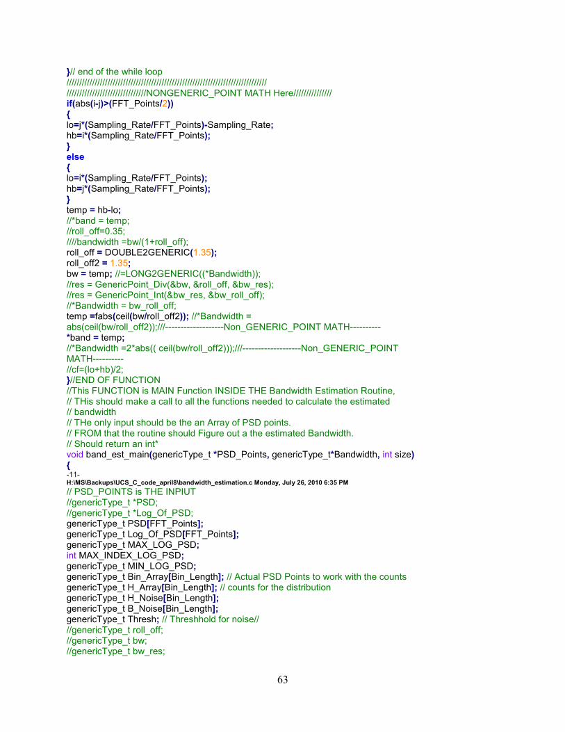
63

}// end of the while loop ////////////////////////////////////////////////////////////////////////////// ///////////////////////////////NONGENERIC_POINT MATH Here/////////////// if(abs(i-j)>(FFT_Points/2)) { lo=j*(Sampling_Rate/FFT_Points)-Sampling_Rate; hb=i*(Sampling_Rate/FFT_Points); } else { lo=i*(Sampling_Rate/FFT_Points); hb=j*(Sampling_Rate/FFT_Points); } temp = hb-lo; //*band = temp; //roll_off=0.35; ////bandwidth =bw/(1+roll_off); roll_off = DOUBLE2GENERIC(1.35); roll_off2 = 1.35; bw = temp; //=LONG2GENERIC((*Bandwidth)); //res = GenericPoint_Div(&bw, &roll_off, &bw_res); //res = GenericPoint_Int(&bw_res, &bw_roll_off); //*Bandwidth = bw_roll_off; temp =fabs(ceil(bw/roll_off2)); //*Bandwidth = abs(ceil(bw/roll_off2));///-------------------Non_GENERIC_POINT MATH---------- *band = temp; //*Bandwidth =2*abs(( ceil(bw/roll_off2)));///-------------------Non_GENERIC_POINT MATH---------- //cf=(lo+hb)/2; }//END OF FUNCTION //This FUNCTION is MAIN Function INSIDE THE Bandwidth Estimation Routine, // THis should make a call to all the functions needed to calculate the estimated // bandwidth // THe only input should be the an Array of PSD points. // FROM that the routine should Figure out a the estimated Bandwidth. // Should return an int* void band_est_main(genericType_t *PSD_Points, genericType_t*Bandwidth, int size) { -11- H:\MS\Backups\UCS_C_code_april8\bandwidth_estimation.c Monday, July 26, 2010 6:35 PM

// PSD_POINTS is THE INPIUT //genericType_t *PSD; //genericType_t *Log_Of_PSD; genericType_t PSD[FFT_Points]; genericType_t Log_Of_PSD[FFT_Points]; genericType_t MAX_LOG_PSD; int MAX_INDEX_LOG_PSD; genericType_t MIN_LOG_PSD; genericType_t Bin_Array[Bin_Length]; // Actual PSD Points to work with the counts genericType_t H_Array[Bin_Length]; // counts for the distribution genericType_t H_Noise[Bin_Length]; genericType_t B_Noise[Bin_Length]; genericType_t Thresh; // Threshhold for noise// //genericType_t roll_off; //genericType_t bw; //genericType_t bw_res;

64

//int bw_roll_off; //float roll_off2; //errorCodeEnum_t res; int i=0; //Just for now, int digital =1; // assume that the bandwidth of all digital signals //PSD= (genericType_t*)malloc(size*sizeof(genericType_t)); //Log_Of_PSD = (genericType_t*)malloc(size*sizeof(genericType_t)); //initializations the PSD Points. MAX_LOG_PSD =INT2GENERIC(0); MAX_INDEX_LOG_PSD=0; MIN_LOG_PSD = INT2GENERIC(0); Thresh =INT2GENERIC(0); for(i=0;i<size;i++) { PSD[i] = INT2GENERIC(0); Log_Of_PSD[i] = INT2GENERIC(0); // Initialize the Log of the PSD to All zeros } -12- H:\MS\Backups\UCS_C_code_april8\bandwidth_estimation.c Monday, July 26, 2010 6:35 PM

for(i=0;i<size;i++) { PSD[i] = PSD_Points[i]; // The address of one is assigned to the address of the other } for(i =0;i<Bin_Length;i++) //initialize the values back to zero; { H_Array[i] = INT2GENERIC(0); Bin_Array[i] = INT2GENERIC(0); H_Noise[i] = INT2GENERIC(0); B_Noise[i] = INT2GENERIC(0); }// Log_10_PSD(PSD, Log_Of_PSD, size);// Calculate the Log of the PSD MAX_L (Log_Of_PSD,&MAX_LOG_PSD, &MAX_INDEX_LOG_PSD,size); MIN_L (Log_Of_PSD, &MAX_LOG_PSD, &MAX_INDEX_LOG_PSD, &MIN_LOG_PSD, size); Histogram_PSD(Log_Of_PSD, &MAX_LOG_PSD, &MIN_LOG_PSD, Bin_Array, H_Array, size); Noise_Vectors(Bin_Array,H_Array, H_Noise, B_Noise, &Thresh, size, digital); Bandwidth_Estimation(Log_Of_PSD,&Thresh,Bandwidth, size); free(PSD); free(Log_Of_PSD); }// End of the Function -13-

65

Appendix B

Source Code Listing for Symbol Timing Estimation H:\MS\Backups\UCS_C_code_april8\Symbol_Timing.c Monday, July 26, 2010 6:32 PM

#include "Symbol_Timing.h" #include "lyrtech_init.h" ////*********Variable Array Sizes for the use********************************************** //#define Sampling_Rate 2000000 //Sammpling Rate is 2M for current applications #define NUM_SAMP 128 #define Sampling_Rate 1600000 // Sampling rate for ANRITSU DATA is 1.6M# #ifndef step_sr #define step_sr 100 //change the step sr for searching range #endif // range is normally 1; Step_sr normally 100 #ifndef Range #define Range 1 //change the step sr for searching range #endif // range is normally #define Vector_Size_Resample_const 2048 // This is the size of the The Resampled Contesllation // So far I have seen Interpolation Factors on the orders of 250;-->250000+ points for data on samples of 1024 #define Vector_Size_Resample 60000 // This is the size of the vector to hold Upsampled and Filterd Data //(Conv_Size = Vector_Size_Resample + FIR_Size); #define Conv_Size 62000 //This has to be the size of FIR_Size and Vector_Size Resample #define Limiter_Len 2000 //*** CHANGE THIS to MAX value for the size for a limiter function /////////----------------------- #define FIR_Size 512 // This is the size of the Filter used for Resampling( MAX filter size) #define num_fft_conv 1024 // This is the fft size to use for filtering. Affects speed // the fft size should be less the the FIR_SIZE ////////------------------------ //---------SymbolSearching Variables that might need to be bigger for to support full func-- // In Case of a Crash, or depending on Program Memory Restrictions // Experiment with these lengths and Rebuild #define inte_size 200 #define elg_len 2048 #define re_elg_len 2048 #define elg1_len 256 #define conv_cons_len 256 #define var_all_len 2048 // This is usually 21*36 #define try_bw_len 200 // Ususally 21 #define max_min_len 200 // About 21 in matlab verison #define two_d_array_len 400 // This goes back to storing and accessing elements as a 2d array #define g_len 100 // This is the size of the array for the QAM searching section #define second_var_len 200 // *** Check the appropriate size of this not sure what it is -1- H:\MS\Backups\UCS_C_code_april8\Symbol_Timing.c Monday, July 26, 2010 6:32 PM

supposed to be as of now static const genericType_t Signal_Processing_Constant_Value_1 = INT2GENERIC (1); static const genericType_t Signal_Processing_Constant_Value_0 = INT2GENERIC (0); //-------END of DEFINE Statements for SYmbol Timing Variables------------------------------ // THings to check // 1) Check out the generic convolution. size of output // 2) /* These are the Funtion Calls that need to be inititated in Main. Possibly Copy and Paste the code below in Main(Appropriate Section) to get it to work: //Symboltiming Data type Definitions

66

genericComplexType_t *Complex_Samples_Data[NUM_SAMP]; // example Number of samples passed to DSP from FPGA //Symboltimming Function Calls where appropriate convertFromWANNSamplesToGenericSamples(wannInputSamples, Complex_Samples_Data, NUM_SAMP); // convert the samples to complex I+jQ format // Complex_Samples_Data is of generic */ //FIR routine taken from TEXAS INSTRUMENTS ////////////////////////// Funtions for SymbolTiming////////////////////////////////// //This is the Function to rationlize given Interpolation and Decimatian factors // Basically reduce them to the Lowest Terms //WORKS void RAT(long *m, long *n) { while(*m!=*n) // There is no decimal point so no need for Generic Point Math { if( *m > *n) *m= *m - *n; //large - small , store the results in large variable else *n= *n - *m; }// end the while Loop /// Remeber to divide I and D by M; -2- H:\MS\Backups\UCS_C_code_april8\Symbol_Timing.c Monday, July 26, 2010 6:32 PM

}// End of the RAT function. // This function does UPSAMPLING by zero insertion. //Inserts N-1 zeros inbetween each element of the array //size is the length of the input sample.( The total number of input samples or IQponts) // In reality it does not insert the zeros but keeps track of how many zeros are inbetween each element //WORKS void Up_Sample(genericComplexType_t *constellation_points, long Interpolation_Factor, genericComplexType_t *Up_Vector,long *Up_Length, int size) { int total_zeros = Interpolation_Factor -1;// insert N-1 zeros between input samples int interp = Interpolation_Factor; int input_length = size; // size of the incoming vecotr of constellation points. eg 1024 int i =0; // This is the for loop iterator; int j=0; int output_length=0; // THis is how big the output or UPvector is going to be // output_length = ceil(input_length * Interpolation_Factor); // This int arithmetic/ No need for gneric type output_length = ceil(input_length * (Interpolation_Factor)); *Up_Length = output_length; // The size out_put Vector will be output Length //start_addr = temp_vector; for(i =0;i< output_length;i++) { Up_Vector[i].real = Signal_Processing_Constant_Value_0; Up_Vector[i].imag = Signal_Processing_Constant_Value_0; } //temp_vector = start_addr;// Restart the pointer at the base address // j=0; for (i= 0; i< output_length ;i=i+interp) // Go throuh and reinstert the acual constellation points back into

67

{ // Temp_vector. Up_Vector[i].real = constellation_points[j].real; Up_Vector[i].imag = constellation_points[j].imag; j++; }// The end of the foor loop }// END of of UP_SAMPLE // The convolution using the inputside algorithm. //WORKS void Convolution_Input_Side(genericType_t *input1, genericType_t *input2, int size1, int size2, int output_size, genericType_t *output) -3- H:\MS\Backups\UCS_C_code_april8\Symbol_Timing.c Monday, July 26, 2010 6:32 PM

{ int i,j =0; int total_size; int iterator =0; int al; genericType_t Temp_result[Conv_Size]; genericType_t input_prod; genericType_t intermediate; genericType_t a; // These are the variables to perform the convolution math math. genericType_t b; genericType_t c; errorCodeEnum_t res; total_size =(size1+size2)-1; for(i=0;i<total_size;i++) { Temp_result[i] =INT2GENERIC(0); }// end of initialzation loop for(i = 0; i< size1;i++) { for(j=0;j< size2;j++) { // Temp_result[i+j]=Temp_result[i+j] + (input1[i] * input2[j]); iterator = i+j; a = input1[i]; b = input2[j]; c = Temp_result[iterator]; res =GenericPoint_Mult(&a, &b,&input_prod); res =GenericPoint_Add(&c, &input_prod, &intermediate); Temp_result[iterator] = intermediate; iterator =0; }// inner loop }// End of Outer loop for(i=0;i<output_size;i++) { output[i]=INT2GENERIC(0); } for(i=0;i<output_size;i++) { output[i]=Temp_result[i]; } -4- H:\MS\Backups\UCS_C_code_april8\Symbol_Timing.c Monday, July 26, 2010 6:32 PM

}// End of Function // Convolve a generic_Type with a generic_Complex_type

68

// ***Works void Convolution_Input_Side_Complex(genericType_t *input1, genericComplexType_t *input2, int size1, int size2, int output_size, genericComplexType_t *output) { genericType_t conv_input[Vector_Size_Resample]; genericType_t conv_output[Conv_Size]; int i,j; for(i=0;i<size2;i++) { conv_input[i] = input2[i].real; // copy the contetns of the complex input } Convolution_Input_Side(input1, conv_input,size1, size2, output_size, conv_output); for(i=0;i<output_size;i++) { output[i].real =conv_output[i]; } for(i=0;i<size2;i++) { conv_input[i] = input2[i].imag; // copy the contetns of the complex input } Convolution_Input_Side(input1, conv_input,size1, size2, output_size, conv_output); for(i=0;i<output_size;i++) { output[i].imag =conv_output[i]; } }// End of the Convolution_Input_Side_Complex //THIS IS THE GENERICPOINT CONVOLUTION --OUTPUTSIDE ALGORITHM // Input 3 is the filter // Input 1 is the data void Conv(genericType_t *inputsamples1, genericType_t *filt,int input_size, int taps, genericType_t *result) { -5- H:\MS\Backups\UCS_C_code_april8\Symbol_Timing.c Monday, July 26, 2010 6:32 PM

int i,j; int output_size; errorCodeEnum_t res = NO_MATH_ERROR; genericType_t temp; genericType_t element; genericType_t out; output_size = input_size + taps - 1; for (i = 0; i < output_size; i++) /// Go through each element of the output { result[i] =Signal_Processing_Constant_Value_0; for (j = 0; j < taps; j++) //multiply and accumulate for each output element { // 0 to taps if( ((i-j)<0)||((i-j)>=input_size) ) { //Do Nothing Here } else { element = inputsamples1[i-j]; GenericPoint_Mult(&filt[j], &element , &temp); GenericPoint_Add(&temp, &result[i], &out);

69

result[i] = out; ; } } }// end of big for }// end of the G Conv for Sujits Code void Conv_Complex(genericComplexType_t *input_samples, genericType_t *filt,int input_size, int taps, genericComplexType_t *result) { genericType_t conv_input[Vector_Size_Resample]; // THe biggest size sample to convolve is 1024 for the costellation points genericType_t conv_output[Conv_Size]; int output_length; int i; output_length = input_size+ taps - 1; for(i=0;i<input_size;i++) { conv_input[i] =input_samples[i].real; } -6- H:\MS\Backups\UCS_C_code_april8\Symbol_Timing.c Monday, July 26, 2010 6:32 PM

Conv(conv_input, filt,input_size,taps, conv_output); for(i=0;i<output_length;i++) { result[i].real = conv_output[i]; } for(i=0;i<input_size;i++) { conv_input[i] =input_samples[i].imag; } Conv(conv_input, filt,input_size,taps, conv_output); for(i=0;i<output_length;i++) { result[i].imag = conv_output[i]; } }// end of function ///// The overlap add method//////// //// FFT CONVOLUTION WITH THE OVERLAPP ADD METHOD //// THis is for fast filtering of large amounts of data //// with large filters //// THE FFT SIZE must be specified in the Macros above void FFT_Filter(genericType_t *input_data, genericType_t *filter, genericType_t *result,int input_size, int filter_size) { int output_length; // This is the size int N_FFT; // N is the number of FFT points to use for the convolution int L; // L is block length int i,j; // iterators genericComplexType_t filter_complex[FIR_Size]; //this variable is hold a complex version of the filterdata genericComplexType_t input_complex[Vector_Size_Resample]; // the input sample may be very big errorCodeEnum_t res; DSASignalProcessingType_t dsaVariable; genericComplexType_t twiddleFactors[num_fft_conv]; genericComplexType_t window[num_fft_conv]; genericComplexType_t B [num_fft_conv]; // this holds FFT of the FILTER genericComplexType_t dst[num_fft_conv]; // variable to hold calculations -7-

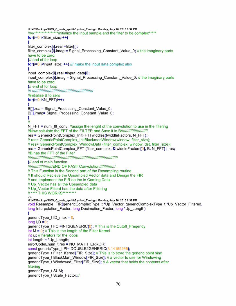
70

H:\MS\Backups\UCS_C_code_april8\Symbol_Timing.c Monday, July 26, 2010 6:32 PM

//////****************initialize the input sample and the filter to be complex***** for(i=0;i<filter_size;i++) { filter_complex[i].real =filter[i]; filter_complex[i].imag = Signal_Processing_Constant_Value_0; // the imaginary parts have to be zero; }// end of for loop for(i=0;i<input_size;i++) /// make the input data complex also { input_complex[i].real =input_data[i]; input_complex[i].imag = Signal_Processing_Constant_Value_0; // the imaginary parts have to be zero; }// end of for loop /// ///////////////////////////////////////////////////////// //initialize B to zero for(i=0;i<N_FFT;i++) { B[i].real= Signal_Processing_Constant_Value_0; B[i].imag= Signal_Processing_Constant_Value_0; } // N_FFT = num_fft_conv; //assign the lenght of the convolution to use in the filtering //Now caltulate the FFT of the FILTER and Save it in B///////////////////////// res = GenericPointComplex_InitFFTTwiddles(twiddleFactors, N_FFT); // res= GenericPointComplex_InitBlackmanWindow(window, filter_size); // res= GenericPointComplex_WindowData (filter_complex, window, dst, filter_size); res = GenericPointComplex_FFT (filter_complex, &twiddleFactors[0], B, N_FFT) | res; //B has the FFT of the Filter //////////////////////////////////////////////////////////////////////////////////// }// end of main function ///////////////////////END OF FAST Convolution/////////////// // This Function is the Second part of the Resampling routine // It should Recieve the Upsampled Vector data and Design the FIR // and Implement the FIR on the in Coming Data // Up_Vector has all the Upsampled data // Up_Vector Filterd has the data after Filtering // **** THIS WORKS********* -8- H:\MS\Backups\UCS_C_code_april8\Symbol_Timing.c Monday, July 26, 2010 6:32 PM

void Resample_FIR(genericComplexType_t *Up_Vector, genericComplexType_t *Up_Vector_Filtered, long Interpolation_Factor, long Decimation_Factor, long *Up_Length) { genericType_t ID_max = 0; long I,D =0; genericType_t FC =INT2GENERIC(0); // This is the Cutoff_Freqency int M = 0; // This is the length of the Filter Kernel int i,j; // Iterators for the loops int length = *Up_Length; errorCodeEnum_t res = NO_MATH_ERROR; const genericType_t PI= DOUBLE2GENERIC(3.14159265); genericType_t Filter_Kernel[FIR_Size]; // This is to store the generic point sinc genericType_t BlackMan_Window[FIR_Size]; // a vector to use for Windowing genericType_t Windowed_Filter[FIR_Size]; // A vector that holds the contents after filtering genericType_t SUM; genericType_t Scale_Factor;//

71

genericType_t Max_H; genericType_t one; genericType_t conv_input1[Vector_Size_Resample]; // These are variables to use in the convoltution for filtering genericType_t conv_input2[Vector_Size_Resample]; genericType_t conv_output1[Vector_Size_Resample]; genericType_t conv_output2[Vector_Size_Resample]; I = Interpolation_Factor; D = Decimation_Factor; ID_max = I; if(ID_max > D) { ID_max =I; } else { ID_max =D; // Find the Maximum Between I and D } ///////////////////////////////////////////////////////////////////////////////////////////////// ///////////////// //FC = 1/D; %Set the cutoff frequency (between 0 and 0.5) //FC = 1.0/ID_max; res=GenericPoint_Div(&Signal_Processing_Constant_Value_1, &ID_max, &FC); //****************************************************************************** -9- H:\MS\Backups\UCS_C_code_april8\Symbol_Timing.c Monday, July 26, 2010 6:32 PM

M = 2*ID_max*10; // 'Set filter length ( Experiment With Different Filter Lengths) //M = FIR_Size; // You can Fix the filter Length for less calculations // And less smooth data. EXPERIMENT WITH THE RESULT // //******************************************************************************** if(M<=FIR_Size) { // Do nothing use the current M } else { M =FIR_Size; } ///////////////////////////////////////////////////////////////////////////////////////////////// /////////////// for(i=0;i<M;i++) // THis part of code follows method 1 of Matlab code resample_script.m for FIR, method 2 for blackman { if((i - (M/2))==0) { Filter_Kernel[i] = DOUBLE2GENERIC(sin(PI*FC)); // Avoid a devidide by zero } else { //filter_kernel(i) = sin(PI*FC * (i-M/2)) / (PI*FC*(i-M/2)); //*(Filter_Kernel+i) = DOUBLE2GENERIC(sin(PI*FC*(i-M/2)) / (PI*FC*(i-M/2))); // Check this for Filter_Kernel[i] = DOUBLE2GENERIC(sin(PI*FC*(i-M/2)) / ((i-M/2))); // Check this for } //black1(i) = (42 - 50*cos((2*pi*i)/M) + 8*cos((4*pi*i)/M))/100;

72

BlackMan_Window [i] =DOUBLE2GENERIC((42 - 50*cos((2*PI*i)/M) + 8*cos((4*PI*i)/M))/100); // }// END of THE GENERATION FOr the Filter KERNEL and THE Blackman WINDOW for(i=0;i<M;i++)//BlackMan WINDOW the SINC pulse to Create a WINDOWED FILTER KERNEL { //filter_wind = filter_kernel.*black1; res= GenericPoint_Mult( &Filter_Kernel[i], &BlackMan_Window[i], &Windowed_Filter[i]); }// Continue from here with Normalization ETC // Normalize the Filter to a Gain of 1 at DC SUM = DOUBLE2GENERIC(0); for(i=0;i<M;i++) { -10- H:\MS\Backups\UCS_C_code_april8\Symbol_Timing.c Monday, July 26, 2010 6:32 PM

//SUM = SUM + *(windowed filter +i); res = GenericPoint_Add(&SUM,&Windowed_Filter[i],&SUM); }// end of the for loop for(i=0;i<M;i++) { //*(windowed_filter + i) = *(Windowed Filter +i)/SUM; res = GenericPoint_Div(&Windowed_Filter [i],&SUM, &Windowed_Filter[i]); } // THIS MAY or MAY bot be needed Max_H= DOUBLE2GENERIC(0); for(i=0;i < M; i++) { if(Windowed_Filter[i]>Max_H) { Max_H =Windowed_Filter[i]; } } //Scale_Factor = floor(1/Scale_Factor); one =DOUBLE2GENERIC(1); res = GenericPoint_Div(&one, &Max_H, &Scale_Factor); for(i=0;i< M;i++) { //*(Windowed_Filter + i) = *(Windowed_Filter +i)*Scale_Factor; res = GenericPoint_Mult((&Windowed_Filter[i]),&Scale_Factor,(&Windowed_Filter[i])); //res = GenericPoint_Mult((Filter_Kernel +i),&Scale_Factor,(Filter_Kernel +i)); } for(i=0;i<length;i++) { conv_input1[i] = Up_Vector[i].real; conv_input2[i] = Up_Vector[i].imag; } /////////Next Up Convolve the input signal with the filter to perform the filtering //Convolution_Input_Side(conv_input1, Windowed_Filter,length, M,length, conv_output1); //Convolution_Input_Side(conv_input2, Windowed_Filter,length, M,length, conv_output2); Conv(conv_input1, Windowed_Filter,length, M, conv_output1); Conv(conv_input2, Windowed_Filter,length, M, conv_output2); for(i=0;i<length;i++) { Up_Vector_Filtered[i].real=conv_output1[i]; Up_Vector_Filtered[i].imag=conv_output2[i]; -11- H:\MS\Backups\UCS_C_code_april8\Symbol_Timing.c Monday, July 26, 2010 6:32 PM

}

73

}// End of the filtering of Resample function //THis is the down_sample function, This is the 3rd part of the resampling routine // UP_Vector should contain the data elements after Filtering. // Decimation Factor holds the value to down sample by // Constellation Points Resampled has the values that // after the entire resampling process. // Function should keep every Nth element of the array // starting from the first element. N represent the integer value // the Decimation Factor ///WORKS********************* void Down_Sample(genericComplexType_t *Up_Vector_Filtered, long Decimation_Factor, genericComplexType_t *Constellation_Points_Resampled, long *Up_Length, int *Down_Length ) { long length = *Up_Length; // This is the incoming size of the array int i,j =0; // iterator for a for loop *Down_Length = ceil(length/ Decimation_Factor); for(i=0; i<*Down_Length; i++) { Constellation_Points_Resampled[i].real = INT2GENERIC(0); Constellation_Points_Resampled[i].imag = INT2GENERIC(0); } j=0; for(i=0; i<*Down_Length; i++) { Constellation_Points_Resampled[i].real =Up_Vector_Filtered[j].real ; Constellation_Points_Resampled[i].imag =Up_Vector_Filtered[j].imag; j=j+ Decimation_Factor; // Pick every jth point and throwing away the rest. } }// This is the end of the function //THIS WORKS. THIS CALLS THE FUNCTIONS ABOVE void Resample(genericComplexType_t *constellation_points, genericComplexType_t * constellation_points_resampled, long Interpolation_Factor, long Decimation_Factor,int size,int * Down_Length) { genericComplexType_t Up_Vector[Vector_Size_Resample]; // this is the upsampled vector zero insertion genericComplexType_t Up_Vector_Filtered[Vector_Size_Resample]; //Vector After Filtering -12- H:\MS\Backups\UCS_C_code_april8\Symbol_Timing.c Monday, July 26, 2010 6:32 PM

long Up_Length; long m; long n; m= Interpolation_Factor; n = Decimation_Factor; RAT(&m, &n); // Find the Greatest common divider of the 2 numbers Interpolation_Factor = (Interpolation_Factor/ m); // Rationalize the numbers to smaller numbers Decimation_Factor = (Decimation_Factor/ m); // Up_Sample(constellation_points, Interpolation_Factor, Up_Vector, &Up_Length, size); Resample_FIR(Up_Vector, Up_Vector_Filtered, Interpolation_Factor, Decimation_Factor, & Up_Length); Down_Sample(Up_Vector_Filtered, Decimation_Factor, constellation_points_resampled, & Up_Length,Down_Length ); } //Simple function to take the ABS() of a Generic_Complex_type

74

// and Return an GenericType. Calculates the absolute value of each element(real and imaginary parts) //***WORKS**** void ABS_Complex(genericComplexType_t *input, genericType_t *output, int inputlength) { int i =0; genericType_t input_squared_imag; genericType_t input_squared_real; genericType_t input_real; genericType_t input_imag; genericType_t sum_squared; genericType_t abs_value; errorCodeEnum_t res; for(i=0;i<inputlength;i++) { input_real = (input[i].real); input_imag = (input[i].imag); //input_real = ((input+i)->real); //input_imag = ((input+i)->imag); //GenericPoint_Exp2(genericType_t const *p_Base, genericType_t *result); res= GenericPoint_Mult(&input_real,&input_real, &input_squared_real); -13- H:\MS\Backups\UCS_C_code_april8\Symbol_Timing.c Monday, July 26, 2010 6:32 PM

res= GenericPoint_Mult(&input_imag,&input_imag, &input_squared_imag); // GenericPoint_Add(genericType_t const *a, genericType_t const *b, genericType_t *result); res= GenericPoint_Add(&input_squared_real,&input_squared_imag,&sum_squared); //GenericPoint_Sqrt(genericType_t const *p_Square, genericType_t *result); res = GenericPoint_Sqrt(&sum_squared, &abs_value); output[i] = abs_value; abs_value =INT2GENERIC(0); sum_squared =INT2GENERIC(0); }// end of the for loop } // end of the function////////////////////////////////////////////////////////// // this is the limiter function. takes abs value first then carries out the limiter functionality. // COME BACK TO THIS FUNCTION.IT is Called Once at the very end of the symbol_Timer. //. void Limiter_F(genericType_t *input, genericType_t *output, genericType_t level, int size ) { genericType_t x[Limiter_Len]; genericType_t y1[Limiter_Len]; genericType_t sum_x; genericType_t temp_sum_x; genericType_t temp_x_squared; int i; //int temp_mean; genericType_t mean; genericType_t mean_squared; genericType_t standard_mean; genericType_t temp_mean; //genericType_t *std_mean_mean; // variable for the standard_mean/mean // genericType_t R_th[2]; genericType_t R; genericType_t len;

75

genericType_t lim_var_squared;// this the major variable for the comparison in the lim funchtin genericType_t lim_var; genericType_t lim_var_temp; -14- H:\MS\Backups\UCS_C_code_april8\Symbol_Timing.c Monday, July 26, 2010 6:32 PM

errorCodeEnum_t res; // ABS_Complex(input, x, size); // x should have the abs value of the complex input for(i=0;i<size;i++) { x[i] =input[i]; } //level is the number of points in each row or column in QAM //y1=zeros(size(x)); for(i=0;i<size;i++) { y1[i] = INT2GENERIC(0); } //R=[-1]; R = INT2GENERIC(-1); sum_x= INT2GENERIC(0); //-----------------------rms mean for(i=0;i<size;i++) { //Calculate the mean //sum_x=x(i)^2+sum_x;// res=GenericPoint_Mult(&x[i],&x[i], &temp_x_squared); res=GenericPoint_Add(&temp_x_squared, &sum_x, &temp_sum_x); sum_x = temp_sum_x; }// End of For Loop len = INT2GENERIC(size); //mean_x=(sum_x/length(x))^(1/2); res =GenericPoint_Div(&sum_x, &len, &mean_squared); res =GenericPoint_Sqrt(&mean_squared,&mean);//*/ /* for(i=0;i<size;i++)// try the regular mean { res=GenericPoint_Add(&x[i],&sum_x, &temp_sum_x); sum_x = temp_sum_x; }// len = INT2GENERIC(size); res =GenericPoint_Div(&sum_x, &len, &mean_squared); mean = mean_squared;*/ //standard_mean=((4+80+72)/16)^(1/2); standard_mean = DOUBLE2GENERIC(3.1225); //R_th=[5.5,14]; R_th[0] =DOUBLE2GENERIC(5.5); -15- H:\MS\Backups\UCS_C_code_april8\Symbol_Timing.c Monday, July 26, 2010 6:32 PM

R_th[1] =DOUBLE2GENERIC(14.0); for( i=0;i<size;i++) { //*lim_var =(x(i)*standard_mean/mean_x)^2; res =GenericPoint_Mult(&(x[i]), &standard_mean, &lim_var_temp); res=GenericPoint_Div(&lim_var_temp, &mean, &lim_var); res =GenericPoint_Mult(&lim_var,&lim_var, &lim_var_squared); if ( (lim_var_squared < R_th[0]) || (lim_var_squared==R_th[0])) {

76

y1[i]= INT2GENERIC(1); } else if( (lim_var_squared< R_th[1]) && (lim_var_squared>R_th[0]) ) { y1[i]= INT2GENERIC(2); } else { y1[i]=INT2GENERIC(3); } } for(i=0;i<size;i++) { output[i] = y1[i]; } }// end of limiter void ABS_Limiter_F(genericComplexType_t *input, genericType_t *output, genericType_t level, int size ) { genericType_t x[Limiter_Len]; genericType_t y1[Limiter_Len]; genericType_t sum_x; genericType_t temp_sum_x; genericType_t temp_x_squared; int i; //int temp_mean; genericType_t mean; genericType_t mean_squared; genericType_t standard_mean; genericType_t temp_mean; //genericType_t *std_mean_mean; // variable for the standard_mean/mean // genericType_t R_th[2]; -16- H:\MS\Backups\UCS_C_code_april8\Symbol_Timing.c Monday, July 26, 2010 6:32 PM

genericType_t R; genericType_t len; genericType_t lim_var_squared;// this the major variable for the comparison in the lim funchtin genericType_t lim_var; genericType_t lim_var_temp; errorCodeEnum_t res; ABS_Complex(input, x, size); // x should have the abs value of the complex input //level is the number of points in each row or column in QAM //y1=zeros(size(x)); for(i=0;i<size;i++) { y1[i] = INT2GENERIC(0); } //R=[-1]; R = INT2GENERIC(-1); sum_x= INT2GENERIC(0); for(i=0;i<size;i++) { //Calculate the mean //sum_x=x(i)^2+sum_x;//

77

res=GenericPoint_Mult(&x[i],&x[i], &temp_x_squared); res=GenericPoint_Add(&temp_x_squared, &sum_x, &temp_sum_x); sum_x = temp_sum_x; }// End of For Loop len = INT2GENERIC(size); //mean_x=(sum_x/length(x))^(1/2); res =GenericPoint_Div(&sum_x, &len, &mean_squared); res =GenericPoint_Sqrt(&mean_squared,&mean); //standard_mean=((4+80+72)/16)^(1/2); standard_mean = DOUBLE2GENERIC(3.1225); //R_th=[5.5,14]; R_th[0] =DOUBLE2GENERIC(5.5); R_th[1] =DOUBLE2GENERIC(14.0); for( i=0;i<size;i++) { -17- H:\MS\Backups\UCS_C_code_april8\Symbol_Timing.c Monday, July 26, 2010 6:32 PM

//*lim_var =(x(i)*standard_mean/mean_x)^2; res =GenericPoint_Mult(&(x[i]), &standard_mean, &lim_var_temp); res=GenericPoint_Div(&lim_var_temp, &mean, &lim_var); res =GenericPoint_Mult(&lim_var,&lim_var, &lim_var_squared); if ( (lim_var_squared < R_th[0]) || (lim_var_squared==R_th[0])) { y1[i]= INT2GENERIC(1); } else if( (lim_var_squared< R_th[1]) && (lim_var_squared>R_th[0]) ) { y1[i]= INT2GENERIC(2); } else { y1[i]=INT2GENERIC(3); } } for(i=0;i<size;i++) { output[i] = y1[i]; } }// end of limiter //This function should take in and array of values and // Calculate the variance of it. //*****Works Quite Wonderfully void Var(genericType_t *input_array, genericType_t *variance, int input_length) { genericType_t Sum1; genericType_t Sum1_temp; genericType_t Sum2,Sum2_temp; genericType_t T_average; genericType_t input; genericType_t X; genericType_t X_squared; genericType_t length; genericType_t length1; errorCodeEnum_t res; int i; Sum1 = INT2GENERIC(0);

78

Sum1_temp = INT2GENERIC(0); Sum2 = INT2GENERIC(0); T_average = INT2GENERIC(0); X_squared=INT2GENERIC(0); -18- H:\MS\Backups\UCS_C_code_april8\Symbol_Timing.c Monday, July 26, 2010 6:32 PM

X =INT2GENERIC(0); length = INT2GENERIC(input_length); length1 = INT2GENERIC(input_length-1); for(i=0;i<input_length;i++) { input = input_array[i]; // extract each input //sum1 = sum1 + F(i) // add each input to to sum //GenericPoint_Add(genericType_t const *a, genericType_t const *b, genericType_t *result); res = GenericPoint_Add(&Sum1, &input, &Sum1_temp); Sum1= Sum1_temp; }//end of loop // tavg = sum1 /no; //GenericPoint_Div(genericType_t const *a, genericType_t const *b, genericType_t *result); res= GenericPoint_Div(&Sum1,&length, &T_average); for(i=0;i<input_length;i++) { //sum2 = sum2 + (F(i)-tavg)^2; res =GenericPoint_Sub(&(input_array[i]), &T_average, &X); res =GenericPoint_Mult(&X,&X, &X_squared); res = GenericPoint_Add(&Sum2, &X_squared, &Sum2_temp); Sum2= Sum2_temp; }// end of the loop //cvar = sum2 /(no-1) res= GenericPoint_Div(&Sum2,&length1, variance); }// END of the VAriance Function //Find the Max and MAX_INDEX void MAX_F (genericType_t *LOG_Of_PSD, genericType_t *MAX_LOG_PSD, int *MAX_INDEX_LOG_PSD, int size) { int i;// Loop counters to traverse the array pointer *MAX_LOG_PSD = INT2GENERIC(0); *MAX_INDEX_LOG_PSD = INT2GENERIC(0); for (i= 0;i< size;i++) { -19- H:\MS\Backups\UCS_C_code_april8\Symbol_Timing.c Monday, July 26, 2010 6:32 PM

if (*(LOG_Of_PSD+i) > *MAX_LOG_PSD) { *MAX_LOG_PSD = *(LOG_Of_PSD+i); *MAX_INDEX_LOG_PSD = i; } // }// End of For Loop }//END of FUNCTION //Find the Min of a Vector void MIN_F (genericType_t *Log_Of_PSD, genericType_t *MAX_LOG_PSD,

79

int *MAX_INDEX_LOG_PSD, genericType_t *MIN_LOG_PSD, int *MIN_INDEX, int size) { int k;// Loop counters to traverse the array pointer *MIN_LOG_PSD = *MAX_LOG_PSD; // Set it to the MAX then compare it downwards for (k= 0;k< size;k++) { if (*MIN_LOG_PSD > *(Log_Of_PSD+k)) { *MIN_LOG_PSD = *(Log_Of_PSD+k); *MIN_INDEX = k; } // Log_Of_PSD++;// go the next address or element in LoG PSD }// End of For Loop }//END of FUNCTION //----------------------------------------------------------------------------------------------- ------------------ -20- H:\MS\Backups\UCS_C_code_april8\Symbol_Timing.c Monday, July 26, 2010 6:32 PM

// This is one of 2 modules that search for the symbol rate inside the main UCS Routine // Takes est_bw, and constellation points, and the sampling rate and range as the input to the routine // It provides the valunes max_min., second_var, est_sr, and est_sps as outputs // Since this a void function the above variables must be declared as pointers for manipulataion // inside the routine and use outside of the routine. void Symbol_Rate_Searching(genericType_t est_bw, genericComplexType_t *constellation_points, long sampling_rate, int range, genericType_t *max_min, genericType_t *second_var, genericType_t *est_sr, genericType_t *est_sps, genericType_t *tim, genericType_t * max_max_min, genericType_t *max_second_var,int* Qam_Search) { //genericType_t sr = INT2GENERIC(sampling_rate);// Convert the sampling rate to generic type //int step_sr=100; int new_size; errorCodeEnum_t res = NO_MATH_ERROR; long sampling_rate_new, resampling_rate; genericType_t try_bw[try_bw_len]; // a vector of all the possible bandiwidth estmates // This is +- in increments of 100 of the initial bandwidth // estimation //this seeems like 21 elements wide from original code int i,j,b; //iterator variables int x,y; // int try_bw_length; long bw_low; // THis is the lower bound of the range of bandwidth values long est_sps2; // This is integer value of the est_sps to keep as an integer int var_all_length;// interger value for the total number elements that needs to be in the array //int var_all_iterator; // an interger value to iterate through a one dimeninal array as if it was a 2 dimensional array long up_factor,down_factor; // These are the I and D for Inter/decim to use in the vector resampling genericComplexType_t constellation_points_new[Vector_Size_Resample_const];// this is values

80

for the constellation points after resampling genericType_t inte[inte_size]; // This is a vector used in smoothing out. genericType_t elg1[elg1_len]; // this has the abs(conv_cons) genericType_t elg[elg_len];// abs(conv_cons)/est_sps genericType_t re_elg[re_elg_len]; -21- H:\MS\Backups\UCS_C_code_april8\Symbol_Timing.c Monday, July 26, 2010 6:32 PM

//---------------------------------------------------------------- genericComplexType_t conv_cons[conv_cons_len]; // how long should this be. int conv_cons_length; //------------------------------------------------------------------ genericType_t variance; genericType_t var_all[var_all_len]; // this all the row by row var calculations in the entire run *GM genericType_t var_all_aligned[var_all_len]; // this all the row by row var calculations in the entire run *GM genericType_t Row_Focus[two_d_array_len]; // This is holds a row from the "2D Array"; genericType_t Row_Focus_Qam[two_d_array_len]; // This is holds a row from the "2D Array"; genericType_t var_row[two_d_array_len]; // this is a row of variance calulations for each run of the main loop genericType_t var_row_qam[two_d_array_len]; // this is a row of variance calulations for each run of the main loop //up to GM genericType_t max_var; // this all the row by row var calculations in the entire run genericType_t min_var; int max_var_index; int min_var_index; genericType_t max_var_all; // this all the row by row var calculations in the entire run genericType_t min_var_all; genericType_t group_index[g_len]; // for use in the QAM section genericType_t g1[g_len]; genericType_t g2[g_len]; genericType_t g3[g_len];// these variabkes are also for the Qam; int g1_next; int g2_next; int g3_next; genericType_t var_g1; genericType_t var_g2; genericType_t var_g3; genericType_t var_g1_prod; genericType_t var_g2_prod; genericType_t var_g3_prod; genericType_t var_qam_temp; // temp variable for use in this genericType_t var_g_prod_sum; genericType_t var_qam; -22- H:\MS\Backups\UCS_C_code_april8\Symbol_Timing.c Monday, July 26, 2010 6:32 PM

genericType_t level; int elg_length; int col,row, num_rows,num_cols,index; // these variables are used for using the 1D array as a // 2D array; int second_i; int ggg; int kkk; int posi; int tim_max; int array_iterator=0;

81

int var_all_iterator=0; int var_all_width; genericType_t var_all_2d[100][100]; genericType_t re_elg_2d[100][100]; genericType_t Row_Focus2D[two_d_array_len]; genericType_t tim2,est_sr2; //////////////////////////////////////////////////////////Code sequence for Symbol checked by GM //est_sps=round(sampling_rate/est_bw)); //sps means samples per symbol. /This value is set and is the value that is returned.-- Therefore this can be calculated in the main symbol_timing_file est_sps2 = sampling_rate/est_bw; *est_sps = LONG2GENERIC((sampling_rate/est_bw)); // If there is any problem with this // Convert back to Generic point Math and retry ///res =GenericPoint_Div(&sr, &est_bw, est_sps); //% step_sr also seen in the symbol_timing_m //try_bw=est_bw-range*1000:step_sr:est_bw+range*1000; % create a vectore try_bw from est_bw-(range*1000) , // increments of 100, to est_bw +(range)*1000 try_bw_length =(est_bw + range*1000)-(est_bw- range*1000); try_bw_length = (try_bw_length/step_sr) + 1 ; bw_low = (est_bw-(range*1000)); for(i=0;i<try_bw_length;i++) { -23- H:\MS\Backups\UCS_C_code_april8\Symbol_Timing.c Monday, July 26, 2010 6:32 PM

try_bw[i] = bw_low; // This pointer should have and array of bandwidths to search. bw_low = bw_low+step_sr; }// The end of the for loop sampling_rate_new=sampling_rate; //% assign the old sampling rate to the new one var_all_length = try_bw_length * est_sps2; // //var_all=zeros(length(try_bw),est_sps); // %create y* x array of zeros for max_min //max_min=zeros(1,length(try_bw)); // %create 1* x array of zeros for max_min //INITIALIZE THE var_all and max_min to all zeros for(i=0;i<var_all_length;i++) { var_all[i]= INT2GENERIC(0); }// end of the for loop for(i=0;i<try_bw_length;i++) { max_min [i]= INT2GENERIC(0); //GM }// end of the for loop for(i=0;i<re_elg_len;i++) { re_elg[i]= INT2GENERIC(0); }// for(i=0;i<two_d_array_len;i++) { var_row[i] = INT2GENERIC(0); }

82

// MAIN LOOP of the SYMBOL SEARCHING Begins Here.//-------------------------------------------------------- //What goes in Here??? Lots of JIZZ for(j=0;j<try_bw_length;j++) { // resampling_rate=try_bw(j)*est_sps; //Resampling rate = each element in try_bw* estimated sampling rate // Pick the first element in array of potential bandwithds //res =GenericPoint_Multi(&(try_bw[j]),est_sps, &resampling_rate); resampling_rate = try_bw[j]*est_sps2; up_factor =resampling_rate/step_sr; down_factor = sampling_rate_new/step_sr; //NOW THE BIG BANG, RESAMPLE!!!!!. -24- H:\MS\Backups\UCS_C_code_april8\Symbol_Timing.c Monday, July 26, 2010 6:32 PM

Resample(constellation_points, constellation_points_new, up_factor, down_factor,NUM_SAMP , &new_size); /// PSD POINTS is Set Globaly to 1024 //inte=ones(1,est_sps); % Used to integrate incoming data for early late gate Create 1 X est_sps elements of ones for(i=0;i<est_sps2;i++) { inte[i] = INT2GENERIC(1); // initialize everything to a vector of all ones } //----------------------------------------------------------------------------------------------- --------------------- // conv_cons=conv(inte,constellation_points_new) //conv_cons_length = (est_sps2 + new_size)-1; // DOes not need to be generic tupe conv_cons_length = (est_sps2 + new_size)-1; //This Length is based on the rule of COnvolution Conv_Complex(constellation_points_new,inte,new_size,est_sps2,conv_cons); //GM //----------------------------------------------------------------------------------------------- ------------------------ //elg1= abs(conv_cons); //ABS_Complex(genericComplexType_t *input, genericType_t *output, int inputlength); ABS_Complex(conv_cons, elg1, conv_cons_length); //elg=abs(conv_cons)/est_sps; for(i=0;i<conv_cons_length;i++) { //GenericPoint_Div(genericType_t const *a, genericType_t const *b, genericType_t *result); res=GenericPoint_Div(&elg1[i], est_sps, &elg[i]); }// end of the for loop //elg_length=floor(length(elg)/est_sps)*est_sps;===> elg_length = floor((conv_cons_length/est_sps2)*est_sps2); //UPTO GM //-------------------------------------------------------------------- // re_elg=reshape(elg(1:elg_length),est_sps,[]); // Use a 1D array as a 2D Array. //****PAY ATTENTION TO THE 1D ARRAY AS 2D ARRAY***** // MATLAB USES the COLUMN Major Method, //*****P // NOw remember we are keeping it in the orignal str8 order(row major) // But we will access it as a 2d in column major format********************** // We are saving str8 but accessing as 2d column major********************** //ROW MAJOR -25- H:\MS\Backups\UCS_C_code_april8\Symbol_Timing.c Monday, July 26, 2010 6:32 PM

83

//int A[2][3] = { {1, 2, 3}, {4, 5, 6} }; ROW MAJOR // Saved in Linear Memory as // 1 2 3 4 5 6 // offset = row*NUMCOLS + column //Column MAJOR FORMAT // saved in memory as 1 4 2 5 3 6 //offset = column*NUMROWS + row for(i=0;i<elg_length;i++) { re_elg[i] = elg[i]; // re_elg is saving elg from 0 to elg length. save it as is } num_rows = est_sps2; // THis is for re_elg 80 in test num_cols = (elg_length/num_rows);// this alsofor relg 14 // size of a row is the Number of colums there is //2D version of the Code for(row=0;row<num_rows;row++) { for(col=0;col<num_cols;col++) { re_elg_2d[row][col] = elg[((col)*(num_rows) + (row))]; } } //------------------------------------------------------------------------ if(*Qam_Search == 0) // PSK or "REGULAR" Search { //% Begin to reshape and Evaluate the Samples //var_all(j,:)=var(re_elg,0,2); % var calulates the variance iserting the row by row, varianxce // for example this is 80 wide for(row =0;row<num_rows;row++) // for example this loop wil run 80 times { for(col=0; col<num_cols ; col++) //since re_elg is ex 80 X14.--> end up with 80 variance values { array_iterator=((col)*(num_rows) + (row)); Row_Focus[col]= re_elg[array_iterator ]; //*( re_elg + ( (col)*num_rows + (row) ) ); // access each element row by row Row_Focus2D[col]= re_elg_2d[row][col]; -26- H:\MS\Backups\UCS_C_code_april8\Symbol_Timing.c Monday, July 26, 2010 6:32 PM

} // Now for each row of re_elg that you extract, calculate the variance Var(Row_Focus, &variance, num_cols); var_row[row] =variance; // for example this should have 80 values }// end of nested loop //Next Assign the variance values caluted to the global var_all"2D" array //num rows for re_elg is num_cols for var all. // for example re_elg is 80 x 14. after calculating the variance row by row // there will be 80 variance values. // now var all is 21*80 matrics where eace variace value is inserterd

84

// in a row of var all for(i=0;i< num_rows; i++) // for example from 1 to 80; re_elg_rows are the colums for Var_all { //array_iterator =(i * (try_bw_length) +j); // num rows = try_bw_len, num cols =num_rows var_all[var_all_iterator]= var_row[i]; // so assign each var value to var all var_all_iterator++; //continue filling varall for all runs of the main loop var_all_2d[j][i]=var_row[i]; }// // NOW Remember that above we are saving them in ''2D ORder // Now looking back at the code we dont need var all //max_min(j)=max(var_all(j,:))-min(var_all(j,:)); ex we are goin from 21 by 80 to a 21 by1 MAX_F(var_row, &max_var, &max_var_index, num_rows); MIN_F(var_row, &max_var, &max_var_index, &min_var, &min_var_index, num_rows); res =GenericPoint_Sub(&max_var, &min_var, &max_min[j]); }// End of If Qam_Search else if(*Qam_Search==1) { -27- H:\MS\Backups\UCS_C_code_april8\Symbol_Timing.c Monday, July 26, 2010 6:32 PM

var_qam = INT2GENERIC(0); level = INT2GENERIC(4); // rember re_elg will be say 80*14 matrix saved str8 var_g1_prod =0; var_g2_prod =0; // initializations. var_g3_prod =0; var_g_prod_sum =0; for(i=0;i<est_sps2;i++)//for exmaple run for 80 iterations { for(col=0; col <num_cols; col++) //since re_elf is ex 80 X14.--> end up with 80 variance values { array_iterator =((col)*(num_rows) + (i) ); Row_Focus_Qam [col]= re_elg[array_iterator]; // access each element row by row Row_Focus2D[col]= re_elg_2d[i][col]; // i is the row in this case } Limiter_F(Row_Focus_Qam, group_index, level, num_cols ); g1_next =0; g2_next =0; g3_next =0; for(b=0;b<num_cols;b++) //for example for a 80by14 matrix 14 iterations { //if group_index(b)==1 //g1=[g1 re_elg(i,b)]; if(group_index[b]==(INT2GENERIC(1))) { g1[g1_next] = Row_Focus_Qam[b]; g1_next++; } //elseif group_index(b)==2;

85

// g2=[g2 re_elg(i,b)]; else if(group_index[b] ==(INT2GENERIC(2))) { g2[g2_next] = Row_Focus_Qam[b]; g2_next++; } //else // g3=[g3 re_elg(i,b)]; //end else { g3[g3_next] = Row_Focus_Qam[b]; } }// end of the for -28- H:\MS\Backups\UCS_C_code_april8\Symbol_Timing.c Monday, July 26, 2010 6:32 PM

//if length(g1)~=0 //var_g1=var(g1); //else // var_g1=0; // end if(g1_next>0) { //void Var(genericType_t *input_array, genericType_t *variance, int input_length) Var(g1, &var_g1, g1_next); } else { var_g1 = INT2GENERIC(0); } //if length(g2)~=0 //var_g2=var(g2); //else // var_g2=0; //end if(g2_next>0) { //void Var(genericType_t *input_array, genericType_t *variance, int input_length) Var(g2, &var_g2, g2_next); } else { var_g2 = INT2GENERIC(0); } //if length(g3)~=0 // var_g3=var(g3); // else // var_g3=0; //end if(g3_next>0) { //void Var(genericType_t *input_array, genericType_t *variance, int input_length) Var(g3, &var_g3, g3_next);

86

} else { var_g3 = INT2GENERIC(0); } //remember from current example var all will be a 21* 80 matrix -29- H:\MS\Backups\UCS_C_code_april8\Symbol_Timing.c Monday, July 26, 2010 6:32 PM

//----------------------------------------------------------------------------------------- // var_all(j,i)=(var_g1*(length(g1)-1)+var_g2*(length(g2)-1)+var_g3*(length(g3)-1))/(length(re_elg(1 ,:))-1); // GenericPoint_Mult(genericType_t const *a, genericType_t const *b, genericType_t *result); // GenericPoint_Add(genericType_t const *a, genericType_t const *b, genericType_t *result); // GenericPoint_Sub(genericType_t const *a, genericType_t const *b, genericType_t *result); //GenericPoint_Div(genericType_t const *a, genericType_t const *b, genericType_t *result); var_qam_temp = INT2GENERIC((g1_next-1)); res =GenericPoint_Mult(&var_g1, &var_qam_temp, &var_g1_prod); var_qam_temp = INT2GENERIC((g2_next-1)); res =GenericPoint_Mult(&var_g2, &var_qam_temp, &var_g2_prod); // products of each var and the lengths var_qam_temp = INT2GENERIC((g3_next-1)); res =GenericPoint_Mult(&var_g2,&var_qam_temp,&var_g2_prod); res =GenericPoint_Add(&var_g1_prod,&var_g2_prod,&var_qam_temp); res =GenericPoint_Add(&var_qam_temp, &var_g3_prod, &var_g_prod_sum); var_qam_temp = INT2GENERIC(num_cols-1); res= GenericPoint_Div(&var_g_prod_sum,&var_qam_temp,&var_qam); //------------------------------------------------------------------------------------------ var_row_qam[i] = var_qam;// This should have the }// end of inner for loop for(i=0;i< num_rows; i++) // for example from 1 to 80; { //array_iterator= (i* (try_bw_length) +j); var_all[var_all_iterator] = var_row[i]; // so assign each var value to var all saved row major str8 var_all_iterator++; var_all_2d[j][i]=var_row_qam[i]; }// // NOW Remember that above we are saving them in ''2D ORder -30- H:\MS\Backups\UCS_C_code_april8\Symbol_Timing.c Monday, July 26, 2010 6:32 PM

// Now looking back at the code we dont need var all //max_min(j)=max(var_all(j,:))-min(var_all(j,:)); ex we are goin from 21 by 80 to a 21 by1 MAX_F(var_row, &max_var, &max_var_index, num_rows); MIN_F(var_row, &max_var, &max_var_index, &min_var, &min_var_index, num_rows); res =GenericPoint_Sub(&max_var, &min_var, &(max_min[j])); //% Begin to reshape and Evaluate the Samples //max_min(j)=max(var_all(j,:))-min(var_all(j,:)); }// ********end of else if Qam }//**************************************** end of the for loop ( Main Loop) //min_var_all=min(min(var_all)); //max_var_all=max(max(var_all));

87

MAX_F(var_all, &max_var_all, &max_var_index, var_all_length);// search the entire thing for the max val MIN_F(var_all, &max_var_all, &max_var_index, &min_var_all, &min_var_index, var_all_length ); *est_sr=INT2GENERIC(0); second_i=0; var_all_width=num_rows; //second_var=zeros(1,length(try_bw)-1); for(i=0;i<(try_bw_length-1);i++) { second_var[i] = INT2GENERIC(0); }// end of loop for (kkk=0;kkk<try_bw_length;kkk++) { for (ggg=0; ggg<var_all_width; ggg++ ) { //*************************************************** //index = col *num_rows +row //index = ggg*(try_bw_length) + kkk; index =kkk*var_all_width+ ggg; // var_all is saved in row major str8 order.so use row_major offset if( var_all[index]==min_var_all) { *est_sr=LONG2GENERIC(try_bw[kkk]); posi=kkk; *tim= INT2GENERIC(ggg); -31- H:\MS\Backups\UCS_C_code_april8\Symbol_Timing.c Monday, July 26, 2010 6:32 PM

} if(var_all[index]==max_var_all) { tim_max=ggg; } if(var_all_2d[kkk][ggg]==min_var_all) { est_sr2=LONG2GENERIC(try_bw[kkk]); tim2= INT2GENERIC(ggg); } }// end of the second for if( try_bw[kkk]==*est_sr) { //% plot(var_all(kkk,:),'r'); } else { second_var[second_i]=max_min[kkk]; second_i=second_i+1; // plot(var_all(kkk,:)); }// end of else }// end for MAX_F (max_min,max_max_min,&max_var_index, try_bw_length); // nax_var_index is not important here MAX_F (second_var,max_second_var, &max_var_index, try_bw_length-1); }// End of the function // This is the Main Function of the Symbol Timing // All Initializations function calls etc should be made in this fucntion

88

void Symbol_Timing_F(genericComplexType_t *iq_data, int size, genericType_t *Bandwidth, genericType_t *symbol_rate, genericComplexType_t *symbol_stream, int *mod_order, char *mod_type, int *sr_right) { -32- H:\MS\Backups\UCS_C_code_april8\Symbol_Timing.c Monday, July 26, 2010 6:32 PM

int Qam_Search; // This is a flag created for conciseness in the code. // Allows us to call the PSK Symbol searching routine but // with a special variation for the searching of Qam Symbol rate; //int step_sr=100; int round_index; int range ; int i; int resampled_size; long est_bw; long sampling_rate = Sampling_Rate; long decim,interp; int result1,est_sps2; int result2,est_sr2; int matrix_iterator; genericType_t second_var[second_var_len]; genericType_t est_sr; genericType_t result; genericType_t est_sps; genericType_t tim; genericType_t max_max_min; genericType_t max_second_var; int max_index_second_var; int second_var_count; genericType_t m_sec_var; genericType_t m_sec_var2; genericType_t decimation_rate; genericType_t temp_var; int c_length; int n_rows_main; int n_cols_main; int row, col;// this is row and column iteratiors errorCodeEnum_t res = NO_MATH_ERROR; genericType_t max_min[max_min_len]; genericComplexType_t constellation_points1[NUM_SAMP]; genericComplexType_t constellation_points_new_main[Vector_Size_Resample_const]; genericComplexType_t conv_cons_main[conv_cons_len]; genericType_t inte_main[inte_size]; int conv_cons_main_length; -33- H:\MS\Backups\UCS_C_code_april8\Symbol_Timing.c Monday, July 26, 2010 6:32 PM

genericComplexType_t sample_matrix[re_elg_len]; // SAMPLE_MATRIX IS USED TO DO Reshaping genericType_t limiter_symbol_stream[Limiter_Len]; int lim1; int lim2; int lim3; genericType_t level;

89

int lim_len; genericType_t c_temp; int tim_main; *sr_right =1; // Both these values were initialized to 1 in Matlab range =Range; for(i=0;i<size;i++) { constellation_points1[i]= iq_data[i]; // the iq data } est_bw=ceil(*Bandwidth/1000)*1000; // do we need generic point math here? Qam_Search =0;// DURING THE FIRST RUN, DO NOT SEARCH FOR QAM ///////***** CHange this back to 0 Symbol_Rate_Searching(est_bw, constellation_points1, sampling_rate, range, max_min, second_var, &est_sr,&est_sps, &tim, &max_max_min,&max_second_var,&Qam_Search); temp_var = DOUBLE2GENERIC(1.4); //1.4* max(second_var) => m_sec_var res = GenericPoint_Mult(&max_second_var, &temp_var, &m_sec_var); temp_var = DOUBLE2GENERIC(2.0); res = GenericPoint_Mult(&max_second_var, &temp_var, &m_sec_var2); //2* max(second_var) if( (max_max_min > m_sec_var) && (max_max_min< m_sec_var2) ) { //symbol_searching_qam // Qam_Search =1; Symbol_Rate_Searching(est_bw, constellation_points1, sampling_rate, range, max_min, second_var, &est_sr,&est_sps, &tim, &max_max_min,&max_second_var,&Qam_Search); } while( (max_max_min< m_sec_var2) && (round_index<10) ) { -34- H:\MS\Backups\UCS_C_code_april8\Symbol_Timing.c Monday, July 26, 2010 6:32 PM

//----------------------------------------------------------------------------------------------- - //est_bw= round( bw/1000+2*range*( (-1)^(round_index+1) )*(floor( (round_index+1)/2 )) )*1000; est_bw = ceil(*Bandwidth/1000 + 2*range*( (-1)^(round_index +1)) *floor(( round_index+1)/2 )) * 1000; //------------------come back and fix this round_index=round_index+1; Qam_Search =0; Symbol_Rate_Searching(est_bw, constellation_points1, sampling_rate, range, max_min, second_var, &est_sr,&est_sps, &tim, &max_max_min,&max_second_var,&Qam_Search); temp_var = DOUBLE2GENERIC(1.4); //1.4* max(second_var) res = GenericPoint_Mult(&max_second_var, &temp_var, &m_sec_var); temp_var = DOUBLE2GENERIC(2.0); res = GenericPoint_Mult(&max_second_var, &temp_var, &m_sec_var2); if( (max_max_min > m_sec_var) && (max_max_min)< m_sec_var2 ) { //symbol_searching_qam // Qam_Search =1; Symbol_Rate_Searching(est_bw, constellation_points1, sampling_rate, range, max_min, second_var, &est_sr,&est_sps, &tim, &max_max_min,&max_second_var,&Qam_Search); } }// end of while loop if (round_index==10)

90

{ sr_right=0; } decimation_rate= est_sps; res = GenericPoint_Int(&est_sps, &est_sps2); //result one should have est_sps as and int res = GenericPoint_Int(&est_sr, &est_sr2); //est_sps *est_sr/step_sr interp = (est_sps2* (est_sr2))/step_sr; /// THis is integer Math no need for Generic Math -35- H:\MS\Backups\UCS_C_code_april8\Symbol_Timing.c Monday, July 26, 2010 6:32 PM

decim = sampling_rate/step_sr; // constellation_points_new=resample(constellation_points,est_sr*est_sps/step_sr,sampling_rate/step_ sr); Resample(constellation_points1, constellation_points_new_main, interp, decim,NUM_SAMP, & resampled_size); // size(constellation_points_new); // inte=ones(1,decimation_rate); //inte=ones(1,est_sps); Create 1 X est_sps elements of ones for(i=0;i<est_sps2;i++) // result1-> est_sps { inte_main[i] = INT2GENERIC(1); // initialize everything to a vector of all ones } // /conv_cons=conv(inte,constellation_points_new)/decimation_rate; // c_length=floor(length(conv_cons)/decimation_rate)*decimation_rate; //----------------------------------------------------------------------------------------------- --------------------- // conv_cons=conv(inte,constellation_points_new) //result1 = est_spps conv_cons_main_length = (est_sps2 + resampled_size)-1; // DOes not need to be generic tupe c_length = floor(conv_cons_main_length/(est_sps2))*(est_sps2);//GM //Convolution_Input_Side_Complex(inte_main,constellation_points_new_main,result1,resampled_size,c onv_cons_main_length,conv_cons_main); Conv_Complex(constellation_points_new_main,inte_main,resampled_size,est_sps2, conv_cons_main); //----------------------------------------------------------------------------------------------- ------------------------ //May or may not be needed; for(i=0;i<conv_cons_main_length;i++) { c_temp = conv_cons_main[i].real; res=GenericPoint_Div(&c_temp, &decimation_rate, &result); //conv_cons_main[i].real= c_temp/decimation_rate; conv_cons_main[i].real =result; c_temp = conv_cons_main[i].imag; res=GenericPoint_Div(&c_temp, &decimation_rate, &result); //conv_cons_main[i].real= c_temp/decimation_rate; -36- H:\MS\Backups\UCS_C_code_april8\Symbol_Timing.c Monday, July 26, 2010 6:32 PM

conv_cons_main[i].imag =result; } /// //----------------------------------------------------------------------------- // sample_matrix=reshape(conv_cons(1:c_length),decimation_rate,[]); for(i=0;i<(c_length);i++) { sample_matrix[i] =conv_cons_main[i]; // copy both real and imaginary parts of this

91

} *symbol_rate= est_sr; n_rows_main = est_sps2;// decimation rate = est_sps = result1; n_cols_main = (c_length)/n_rows_main; // symbol_stream=sample_matrix(tim,:); res = GenericPoint_Int(&tim, &tim_main); row = tim_main; for(col=0;col<n_cols_main;col++) { matrix_iterator =col * (n_rows_main) + row; symbol_stream [col]= sample_matrix [matrix_iterator]; } //limiter_symbol_stream=limiter_f(abs(symbol_stream),4); //void ABS_Limiter_F(genericComplexType_t *input, genericType_t* output, genericType_t level, int size ) lim_len = n_cols_main; for(i=0;i<lim_len;i++) { limiter_symbol_stream [i] =INT2GENERIC(0); //initilize the limiter_symbol_stream } level=INT2GENERIC(4); ABS_Limiter_F(symbol_stream, limiter_symbol_stream,level, n_cols_main); lim1=0; lim2=0; lim3=0; for (i=1; i<lim_len;i++) { if (limiter_symbol_stream[i]==INT2GENERIC(1)) { lim1=lim1+1; } else if (limiter_symbol_stream[i]== INT2GENERIC(2)) { lim2=lim2+1; } else { -37- H:\MS\Backups\UCS_C_code_april8\Symbol_Timing.c Monday, July 26, 2010 6:32 PM

lim3=lim3+1; } }// end of for ///[lim1 lim2 lim3]; if ( (lim3 + lim1) >(lim2/2) ) { //*mod_type='QAM'; mod_type[0]= 'Q'; mod_type[1]= 'A'; mod_type[2]= 'M'; mod_type[3]= '-'; *mod_order=16; *symbol_rate= est_sr; } else { // *mod_type='MPSK'//;

92

mod_type[0]= 'M'; mod_type[1]= 'P'; mod_type[2]= 'S'; mod_type[3]= 'K'; *mod_order=4; *symbol_rate= est_sr; } }// end of the main fucntion. */ // All Initializations function calls etc should be made in this fucntion //This function should take in iq_data and and the Estimated Bandwidth and then perform Symbol timing. // mod_order, symbol_stream, and symbol rate are the outputs of the function. // Thise outputs are have to be made available for further processing such // Universal Synchronization; void Sym_Tim_Main(genericComplexType_t *iq_data, genericType_t *Bandwidth_est, int size, int *mod_order, genericComplexType_t *symbol_stream, genericType_t * symbol_rate, char *mod_type) { //Initializations int sr_right; -38- H:\MS\Backups\UCS_C_code_april8\Symbol_Timing.c Monday, July 26, 2010 6:32 PM

//Test Variables/// Delete when done with////////////////////////// // // genericComplexType_t test_input[10]; genericComplexType_t *up; genericComplexType_t *down; genericType_t test_output[10]; genericComplexType_t test_output_complex[20]; genericType_t variance; genericComplexType_t up_vector[Vector_Size_Resample]; genericComplexType_t down_vector[Vector_Size_Resample_const]; genericComplexType_t up_vector_filtered[Vector_Size_Resample]; //short conv_output[Vector_Size_Resample]; short conv_output[30]; //short conv_input1[10] ={2,4,6,8,10,12,14,16,18,20}; genericType_t conv_input1[3] ={.0672,.0371,0}; //genericType_t conv_input2[10] ={1,3,5,7,9,11,13,15,17,19}; short conv_input2[6] ={1,3,5,7,9,11}; long up_length; int down_length; ///////////////////////////////////////////END OF CODE FOR DELETE //Code sequence mod_type[0]='-'; mod_type[1]='-'; mod_type[2]='-'; mod_type[3]='-'; Symbol_Timing_F(iq_data, size, Bandwidth_est, symbol_rate, symbol_stream, mod_order, mod_type, &sr_right); ///////////////////////////////////////////////////////////////////////////////////////////////// -39- H:\MS\Backups\UCS_C_code_april8\Symbol_Timing.c Monday, July 26, 2010 6:32 PM

////////////////// //Lets do some testing // Delete After use START OF DELETE test_input[0].real = 2;

93

test_input[1].real = 4; test_input[2].real = 6; test_input[3].real = 8; test_input[4].real = 10; test_input[5].real = 12; test_input[6].real = 14; test_input[7].real = 16; test_input[8].real = 18; test_input[9].real = 20; test_input[0].imag = 1; test_input[1].imag = 3; test_input[2].imag = 5; test_input[3].imag = 7; test_input[4].imag = 9; test_input[5].imag = 11; test_input[6].imag = 13; test_input[7].imag = 15; test_input[8].imag = 17; test_input[9].imag = 19; //FFT_Filter(conv_input1, conv_input1,conv_output,10, 10); //Conv(conv_input1, conv_input2,10,5, conv_output); // Up_Sample(test_input, 5,up_vector, &up_length,10); // Resample_FIR(up_vector, up_vector_filtered,5,6, &up_length); //Down_Sample(up_vector_filtered, 6,down_vector, &up_length ,&down_length); //Convolution_Input_Side(conv_input1, conv_input2,10,5,14, conv_output); //Convolution_Input_Side_Complex(conv_input1, test_input, 10, 10,19, test_output_complex); // Resample(test_input,down_vector,5, 6,10,&down_length); // up 5, down 6, size 10 //ABS_Complex(test_input, test_output, 10); //Limiter_F(conv_input1, test_output, 4, 2 ); //Var(conv_input1, &variance, 10); // Symbol_Rate_Searching(Bandwidth_est, iq_data, Sampling_Rate, 1, genericType_t *max_min, genericType_t *second_var, genericType_t *est_sr, // genericType_t *est_sps, genericType_t *tim, genericType_t -40- H:\MS\Backups\UCS_C_code_april8\Symbol_Timing.c Monday, July 26, 2010 6:32 PM

*max_max_min, // genericType_t *max_second_var,int* Qam_Search) ////////////////////END OF THE TEST CODE TO BE DELETED //////////////////////////////////////////////////////////////////////////////// }////////////END OF SYMBOL MAIN

symbol timing and coarse classification of phase · pdf filethe system is constructed to run...

Documents