syllabus - atria | e-learning · field and wave electromagnetics , david k cheng , ... 2nd edition,...

Field Theory 10ES36

Dept of E&C, SJBIT 1

SYLLABUS

PART- A

UNIT – 1: ELECTROSTATICS

Experimental law of coulomb, Electric field intensity, Field due to continuous

volume charge distribution, Field of a line charge, Electric flux density, Electric flux

density, Gauss law, Divergence, Vector Operator, Divergence theorem

6 Hours

UNIT – 2: ENERGY & POTENTIAL, CONDUCTORS, DIELECTRICS &

CAPACITANCE

(a).Energy expended in moving a point charge in an electric field, Line integral,

Definition of potential difference and potential, Potential field of a point charge &

system of charges, Potential gradient, Energy density in an electrostatic field.

(b).Current and current density, Continuity of current, metallic conductors,

Conductor properties and boundary conditions for dielectrics, Conductor properties

and boundary conditions for perfect dielectrics, capacitance and examples

8 Hours

UNIT – 3: POISSONS AND LAPLACES EQUATIONS

Derivation of Poisson’s equation and Laplace’s equation, Uniqueness theorem,

Examples of the solutions Laplace Equations and Poisson’s Equations

6 Hours

UNIT – 4: THE STEADY MAGNETIC FIELDS

Biot- savart law, Amphere’s circuitary law, curl, Stoke’s theorem, Magnetic flux

and flux density, Scalar and Vector magnetic potentials.

6 Hours

PART – B

UNIT – 5 : MAGNETIC FORCES, MATERIALS AND INDUCTANCE

(a).Force on a moving charge and differential current element, Force between

differential current elements, Force and Torque on a closed circuit,

(b).Magnetic materials and inductance, Magnetization and permeability, Magnetic

boundary conditions, Magnetic circuits, Potential energy and forces on magnetic

materials, Inductance and mutual inductance

8 Hours

Field Theory 10ES36


UNIT - 6: TIME VARYING MAGENTIC FIELDS AND MAXWELLS

EQUATION

Faraday’s law, Displacement current, Maxwell’s equation in point and integral

form, Retarded potentials.

6 Hours

UNIT - 7: UNIFORM PLANE WAVES

Wave propagation in free space and dielectrics, Poynting’s theorem and wave

power, Propagation in good conductors – (skin effect)

6 Hours

UNIT - 8: PLANE WAVES AT BOUNDARIES AND DISPERSIVE MEDIA

Reflection of uniform plane waves at normal incidence, SWR, Plane wave

propagation in general directions

6 Hours

TEXT BOOK:

1. Energy Electromagnetics, William H Hayt Jr . and John A Buck, Tata

McGraw-Hill, 7th

edition,2006.

REFERENCE BOOKS:

2. Electromagnetics with Applications, John Krauss and Daniel A Fleisch

McGraw-Hill, 5th edition, 1999

3. Electromagnetic Waves And Radiating Systems, Edward C. Jordan and

Keith G Balmain, Prentice – Hall of India / Pearson Education, 2nd

edition,

1968.Reprint 2002

4. Field and Wave Electromagnetics, David K Cheng, Pearson Education Asia,

2nd edition, - 1989, Indian Reprint – 2001.

Field Theory 10ES36


INDEX SHEET

SL.NO TOPIC PAGE NO.

PART – A

UNIT – 1: ELECTROSTATICS 5-16

1 Experimental Law of Coulomb 5

2 Force on a point charge 6

3 Force due to several charges 6

4 Electric field intensity 7

5 Electric Field intensity due to several charges 7

6 Electric Field intensity at a point due to infinite sheet of charge 7

7 Electric Field at a point on the axis at a charges circular ring 9

8 Electric Flux 10

9 Electric Flux Density 11

10 Gauss’s Law 12

11 Application of Gauss Law 14

12 Divergence and Maxwellls First Equation 16

UNIT – 2 : ENERGY AND POTENTIAL, CONDUCTORS,

DIELECTRICS AND CAPACITANCE

20-31

13 Energy expended in moving a point charge in an electric field 20

14 Definition of Potential and Potential difference 21

15 Equipotential surface, Potential field of a point charge 22

16 Potential field of system of charges 23

17 Potential gradient 24

18 Energy density in an electrostatic field 27

19 Potential energy in a continuous charge distribution 28

20 Boundary condition for conductor free space interface 28

21 Boundary condition for perfect dielectric 31

UNIT – 3: POISSON’S AND LAPLACES EQUATIONS 34-36

22 Laplace’s and Poisson’s Equation 34

23 Uniqueness Theorem 35

24 Examples of solution of Laplace’s equation 36

UNIT – 4 :THE STEADY MAGNETIC FIELD 40-50

25 Introduction 40

26 Biot- Savart’s Law 41

27 Amperes Circuital Law 47

28 Application of Amperes law 48

29 Magnetic Flux Density 49

30 Magnetic scalar & vector potentials 50

Field Theory 10ES36


PART – B

UNIT – 5 : MAGNETIC FORCES, MATERIALS AND

INDUCTANCE

54-73

31 Force on a charged particle 54

32 Force between two current elements 56

33 Magnetic Torque and Moment 57

34 Stokes Theorem 59

35 Force on a moving charge due to electric and magnetic fields 59

36 Force on a current element in a magnetic field 60

37 Boundary conditions on H and B 62

38 Scalar magnetic potential 65

39 Vector Magnetic potential 66

40 Force and Torque on a loop or coil 68

41 Materials in magnetic fields 70

42 Inductance 73

UNIT - 6 :TIME VARYING FIELDS AND MAXWELLS

EQUATION 77-86

43 Introduction 77

44 Transformer and motional emf 78

45 Displacement Current 81

46 Equation of continuity for time varying fields 83

47 Maxwells equations for time varying fields 84

48 Maxwells equations for static fields 86

UNIT – 7 :UNIFORM PLANE WAVE

92-113

49 Sinusoidal Time variation 92

50 Wave propagation in a conducting medium 97

51 Wave propagation in a lossless medium 106

52 Wave propagation in Dielectrics 111

53 Polarization 113

UNIT – 8 :PLANE WAVES AT BOUNDARIES AND IN

DISPERSIVE MEDIA

117-121

54 Reflection of uniform plane waves at normal incidence 117

55 Reflection coefficient and transmission coefficient in case of normal

incidence 119

56 Standing Wave Ratio 121

Field Theory 10ES36


UNIT – 1

ELECTROSTATICS

Syllabus:

Experimental law of coulomb, Electric field intensity, Field due to continuous volume

charge distribution, Field of a line charge, Electric flux density, Electric flux density,

Gauss law, Divergence, Vector Operator, Divergence theorem

REFERENCE BOOKS:

1. Energy Electromagnetics, William H Hayt Jr . and John A Buck, Tata

McGraw-Hill, 7th

edition,2006.

2. Electromagnetics with Applications, John Krauss and Daniel A Fleisch

McGraw-Hill, 5th edition, 1999

3. Electromagnetic Waves And Radiating Systems, Edward C. Jordan and Keith

G Balmain, Prentice – Hall of India / Pearson Education, 2nd

edition,

1968.Reprint 2002

4. Field and Wave Electromagnetics, David K Cheng, Pearson Education Asia,

2nd edition, - 1989, Indian Reprint – 2001.

Coulomb’s Law

Coulomb’s law states that the electrostatic force F between two point charges q1 and

q2 is directly proportional to the product of the magnitude of the charges, and

inversely proportional to the square of the distance between them., and it acts along

the line joining the two charges.

Then, as per the Coulomb’s Law,

F kq1q2

Or F = (kq1q2)/(r²) N

Where k is the constant of proportionality whose value varies with the system of units.

R^ is the unit vector along the line joining the two charges.

In SI unit, k= .

Where is called the permittivity of the free space.

It has an assigned value given as =8.834 F/m.

Field Theory 10ES36


Force on a point charge:

The forces of attraction/repulsion between two point charges and (charges

whose size is much smaller than the distance between them) are given by Coulomb’s

law:

where m/F in SI units, and R is the distance between the two charges.

Here, is the force exerted on , and is the force acting on . The unit vector

points from charge 2 toward charge 1. Accordingly, .

Force on Q1 is given by

F1 = Newtons

Force due to several charges

Let there be many point charges q1,q2,q3.........qn at distances r1,r2,r3.....rn from

charge q. The force F1, F2, F3..........Fn at the charges q1,q2,q3...........qn respectively

are:

q{ r + }

F=Fq1+Fq2+Fq3...............

Hence, F= q{ } N

q1

q2

F2

q1

q2

F

1

Field Theory 10ES36

Dept of ECE, SJBIT 7

Electric field intensity

Electric field intensity at any point in an electric field is the force experienced by positive unit

charge placed at that point.

Consider a charge Q located at a point A. At the point B in the electric fields set up by Q, it is

required

To find the electric field intensity E.

Let the charge at B be and let the charge Q be fixed at A. Let r be the distance between A and

B. As per the Coulomb’s Law, the force between Q and q is given by:

F= r N

If it is a unit positive charge, then by definition, F in the above equation gives the magnitude of

the electric field intensity E.

i.e. E=F when

Therefore, the magnitude of the electric field strength is:

E=Q/(4r

Let r be the unit vector along the line joining A and B. Thus, the vector relation between E is

written as:

E=Q/(4 or²) V/m

Electric Field intensity due to several charges

Let there be many point charges q1,q2,q3.........qn at distances r1,r2,r3.....rn be the corresponding

unit vectors. The field E1, E2, E3..........En at the charges q1,q2,q3...........qn respectively are:

r +

E=Eq1+Eq2+Eq3...............

Hence, E=

Electric field intensity at a point due to a infinite sheet of charge

Let us assume a straight line charge extending along Z axis in a cylindrical coordinate

system from -∞ to +∞ as shown in the figure 1.1. Consider an incremental length dl at a point on

the conductor. The incremental length has an incremental charge of dQ= ρl dl= ρldz’ Coulombs.

Considering the charge dQ, the incremental field intensity at point p is given by,

Field Theory 10ES36


Where

,

and

Therefore,

Integrating the above and substituting z’=ρ cot θ, we get

and

Field Theory 10ES36


Electric field intensity at a point due to a infinite sheet of charge:

Let us assume a infinite sheet of charge with surface charge density ρs as shown in the

figure 1.2. Divide the sheet of charge into differential width strips. number of str Consider an

incremental length dl at a point on the conductor. The line charge density ρl= ρs dy’.

The differential Electric field intensity at point P,

adding the effects of all the strips,

Therefore,

Electric field at a point on the axis of charged circular ring:

Let ρ be the charge density of the ring.

So, ρ=dq/dl

dq=ρdl

Electric field due to an infinitely small element = dE = dq/4πεo r² r

Field Theory 10ES36


where r is the unit vector along AP.

dE can resolved into two rectangular components, dEx and dEy. Now, dEx=dEcosθ.

Taking the magnitude of dE from above, the equation becomes,

dEx=

cosθ=

substituting for dq from above, we have;

dEx=

The component dEy is directed downwards. If we consider an element of the ring at a point

diametrically opposite to A, then its dEy component points upwards and hence, cancels with

that due to element A. The dEx components add up.

∫dEy=0.

The total field at P is the sum of the fields due to all the elements of the ring.

Therefore, E=∫dE=∫dEx+∫dEy=∫dEx

E=∫dEx=

=

But, r=(R²+x²)½

Therefore, E= ax

Where, ax is the unit vector along the x axis.

Electric flux:

The concept of electric flux is useful in association with Gauss' law. The electric flux through a

planar area is defined as the electric field times the component of the area perpendicular to the

field. If the area is not planar, then the evaluation of the flux generally requires an area integral

since the angle will be continually changing.

When the area A is used in a vector operation like this, it is understood that the magnitude of the

vector is equal to the area and the direction of the vector is perpendicular to the area.

Field Theory 10ES36


Consider a concentric sphere having radius of ‘a’m charged up to +Q C. This sphere is

then placed in another sphere having a radius of ’b’ m as shown in the figure 1.4.

There is no electrical connection between them. The outer sphere is momentarily

charged, then it found that the charge on the outer sphere is equal to the charge on the inner

sphere. This is depicted by the radial lines. This is referred as displacement flux. Therefore,

Ψ = Q.

Electric flux density:

If +Q C of charge on the inner sphere produces the electric flux of ψ, tthen electric flux ψ

uniformly distributed over the surface area 4Πa2 m

2 , where

a is the radius of the inner sphere.

The electric flux density si given by

Similarly for the outer sphere,

If the inner sphere becomes smaller and smaller retaining a charge of Q C, it becomes a point

charge. The flux density at appoint ‘r’ from the point charge is given by,

Field Theory 10ES36


The electric field intensity due to point charge in free space is given by,

Therefore in free space,

Gauss law:

The Gauss's law states that. "The electric flux passing through any closed surface is equal to the

total charge enclosed by the surface"

For the Gaussian-surface shown in the following figure, the Gauss' law can be expressed

mathematically, .

Where

Ψ = flux passing through the closed surface

§s =1 surface integral

Ds =, flux density (vector quantity) normal to the surface

Q = Total charge enclosed in the surface

Gauss law for charge Q enclosed in a closed surface:

Let Q be the point charge placed at the origin of imaginary sphere in spherical co-ordinate

system with a radius of "a" as illustrated in the figure

Field Theory 10ES36


The electrical field intensity cf the point charge is found to be equal to

Where r = Cl

and we also know that the relation between E and D as,

Therefore from (1) and (2) we get.

at the surface of the sphere,

The differential element of area on a spherical surface is, in spherical coordinate form is given

by,

Then the required integrand

Field Theory 10ES36


Then the integration over the surface as required for Gauss' law.

The limits placed for integral indicate that the integration over the entire sphere in spherical co-

ordinate system on integration we get

Thus we get, comparing LHS of Gauss' law as

,

This indicates that, Q coulombs of electric flux are crossing the surface as the enclosed charge is

Q coulombs.

Application of Gauss law:

In case of asymmetry, we need to choose a very closed surface such that D is almost constant

over the surface. Consider any point P shown in the figure 1.6 located in the rectangular co-

ordinate system.

Field Theory 10ES36


The value of D at point P, may be expressed in rectangular components as,

D=Dx0ax+Dy0ay+Dz0az. . From Gauss law, we have

In order to evaluate the integral over the closed surface, the integral must be broken into six

integrals, one over each surface,

= + .

The surface element is very small & hence D is essentially constant ,

,

Similarly,

and,

.

Therefore collectively,

Field Theory 10ES36


Charge enclosed in volume ∆v,

Divergence:

From Gauss law, we know that,

And applying limits,

The last term in the equation is the volume charge density, ρv.

We shall write it as two separate equations,

And

.

Divergence is defined as,

.

Statement: The flux crossing the closed surface is equal to the integral of the divergence of the

flux density throughout the enclosed volume, as the volume shrinks to zero.

Field Theory 10ES36


Divergence in Cartesian system,

Divergence in Cylindrical system,

Divergence in Spherical system,

Maxwell’s First equation:

From divergence theorem, we have

From Gauss law,

Per unit volume,

As the volume shrinks to zero,

Therefore, div D = ρv.

Field Theory 10ES36


Divergence theorem:

The del operator is defined as a vector operator.

.

In Cartesian coordinate system,

Which is equal to,

.

Therefore,

.

From Gauss law, we have

And by letting,

& .

Hence we have,

Field Theory 10ES36


RECOMMENDED QUESTIONS

1. State Coulomb’s law of force between any 2 point charges & indicate the units of the

quantities involved.

2. Derive the general expression for electric field vector due to infinite line charge using

Gauss law.

3. State and prove Gauss law.

4. Derive the general expression for E at a height h(h<a) , along the axis of the ring charge

& normal to its plane.

5. From gauss law show that ∆.D=σv

6. State and prove divergence theorem for symmetric condition.

7. State and prove divergence theorem for asymmetric condition.

Field Theory 10ES36


UNIT – 2

ENERGY & POTENTIAL, CONDUCTORS, DIELECTRICS AND

CAPACITANCE

Syllabus:

(a).Energy expended in moving a point charge in an electric field, Line integral, Definition of

potential difference and potential, Potential field of a point charge & system of charges, Potential

gradient, Energy density in an electrostatic field.

(b).Current and current density, Continuity of current, metallic conductors, Conductor properties

and boundary conditions for dielectrics, Conductor properties and boundary conditions for

perfect dielectrics, capacitance and examples

REFERENCE BOOKS:

1. Energy Electromagnetics, William H Hayt Jr . and John A Buck, Tata McGraw-Hill, 7th

edition,2006.

2. Electromagnetics with Applications, John Krauss and Daniel A Fleisch McGraw-Hill, 5th

edition, 1999



edition, 1968.Reprint

2002

4. Field and Wave Electromagnetics, David K Cheng, Pearson Education Asia, 2nd edition,

- 1989, Indian Reprint – 2001.

Energy expended in moving a point charge in an electric field

Electric field intensity is defined as the force experienced by unit test charge at a point p. If the

test charge is moved against the electric field, then we have to exert a force equal and opposite to

that exerted by the field and this requires work to be done.

Suppose we need to move a charge fo Q C a distance dl in an electric field E. The force

on Q arising from the electric field is,

The differential amount of work done in moving charge Q over a distance dl is given by,

, as F =QE

Field Theory 10ES36


Thus the work done to move the charge for the finite distance is given by,

Definition of Potential &Potential difference :

Potential difference(V) is defined as the work done in moving unit positive charge from one

point to another point in an electric field.

We know that,

,

Therefore V=W/Q=

VAB signifies potential difference between points A & B and the work done in moving the unit

charge from B to A. Thus B is the initial point & A is the final point.

.

From the previous example, the work done in moving charge Q from ρ= b to ρ= a was,

.

Thus the potential difference between the points a & b is given by,

Absolute electric potential is defined as the work done in moving a unit positive charge from

infinity to that point against the field.

Electric field is defined as force on unit charge.

E= F/Q.

By moving the charge Q aganist an electric field between the two points a & b work is done.

Thus ,

Edl= Fxdl/Q =work/ charge.

This work done per charge is the electric potential difference. Potential difference between points

a and b at a radial distance of ra and rb from a point charge Q is given by,

Field Theory 10ES36


If the potential at point a is VA and at point B is VB, then

.

Equipotential Surface

It is defined as "It is a surface composed of all- points having the same value of potential" on

such surfaces no work is involved in moving a unit charge, hence no potential difference

between any two points on this surface.

Potential field of a point charge

Consider a point charge Q to be placed in the origin of a spherical coordinate system. Consider 2

points A & B as shown in the figure.

Electric Potential difference between A & B, VAB is given by,

dl in spherical co ordinate system is given the figure above and E=Q/ 4Π€r

2.

Therefore,

And

Field Theory 10ES36


Potential field of system of charges: Conservative property

Potential at a point has been defined as the work done in moving unit positive charge from zero

reference to the point. Potential is independent of the path taken from one point to the other.

Potential due to a single charge is given by

V(r)= Q1/ 4Π€R. If Q1 is at r1 & point p at r, then

Potential arising from 2 charges, Q1 at r1 and Q2 at r2, is given by

Potential due to n number of charges, is given by

Or

If point charge is a small element in the continuous volume charge distribution then,

As number of point charges in the volume charge distribution tends to infinity,

Similarly if the point charges takes the form of a straight line then,

Similarly if the point charges takes the form of a surface charge then,

Potential is a function of inverse distance. Hence we can conclude that for a zero reference at

infinity, then:

I Potential due to a single point charge is the work done in moving unit positive charge

from zero reference to the point. Potential is independent of the path taken from one point to the

other

II Potential field due to number of charges is the sum of the individual potential fields

arising from each charge.

Field Theory 10ES36


III. Potential due to continuous charge distribution is found by carrying a unit charge from

infinity to the point under consideration.

is independent on the path chosen for the line integral,

regardless of the source of the E field.

Hence we can conclude that no work is done in carrying a unit positive charge around any closed

path, or

Any field that satisfies an equation of the form above is said to be conservative field

Potential gradient

Potential at any point is given by

Potential difference between 2 points separated by a very short length ∆L along which E

is essentially constant, is given by

In rectangular co ordinate system,

,

As V is a unique function of x,y,z. Then,

.

Since both the expressions are true with respect dx,dy & dz, we can write

Therefore,

Field Theory 10ES36


In rectangular co ordinate system,

Combining all the above equations allows us to use a compact expression that relates E &

V,

Gradient in other coordinate system is as given below,

Field Theory 10ES36


Dipole

Dipole is the name given to 2 point charges of equal magnitude but opposite in sign, separated by

a small distance which is small compared to the distance to point P at which we need to find

electric and potential fields. Dipole is as shown in the figure below,

Let the distance from Q & -Q to P be R1 & R2 respectively, and the distance between the two

charges be‘d’. Total Potential at point P due to Q1 & Q2 is given by,

Since mid-way between the 2 point charges are located at Z=0, R1= R2 & therefore the potential

is zero.

For distant point, R1R2=r2 and R1 & R2 are the approximately parallel as shown in the figure

below

From the figure, R2-R1 =d cos θ;

Therefore,

Field Theory 10ES36


The plane Z=0 is at zero potential. Using gradient relationship in spherical co ordinates,

From the above we obtain,

Or

Energy density in an electrostatic field:

Consider a surface without charge. Bringing a charge Q1 from infinity to any point on the

surface requires no work as there is no field present. The positioning of Q2 at appoint in the field

of Q1 requires an amount of work to be done which is given by

.

Similarly work required to position each additional charge in the field is given by,

Total positioning work = Potential energy of the field

Bringing the charges in the reverse order, the work done is given by,

Adding the 2 energy expressions, we get

For n number of charges,

Field Theory 10ES36


Potential energy in a continuous charge distribution:

For the region with continuous charge distribution, the equation for WE=

By vector identity which is true for any scalar function V & vector D,

,

Then,

.

From Guass law, We can write

and from gradient

Boundary condition for conductor free space interface:

Consider a closed path at the boundary between conductor and a dielectric, such that

∆h→0.

We know that work done in moving a charge over a closed path is zero i.e.,

.

Therefore the integral can be broken up as,

Field Theory 10ES36


.

Let the length from a to b or c to d be ∆W and from a to d or b to c be ∆h , hence we obtain,

.

Hence we obtain E∆W=0 & therefore Et=0

Hence at the conductor dielectric interface tangential component of the electric field intensity is

zero.

Consider a gaussian cylinder of radius ρ and height ∆h at the boundary, Applying Gauss

law,

& then integrating over the distinct surfaces we get

.

Flux experienced by the lateral surface is zero & Flux experienced by the bottom surface is zero

as charge inside the conductor is zero. Therefore

or .

At the conductor dielectric interface normal component of the electric flux density is equal to the

surface charge density.

Field Theory 10ES36


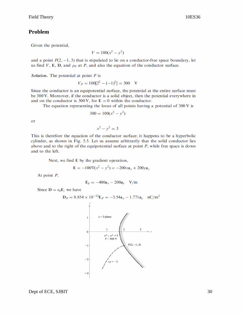
Problem

Field Theory 10ES36


Boundary condition for perfect dielectric:

Consider a closed path abcda at the dielectric dielectric interface & ∆h→0. The work done in

moving a unit charge over a closed path is zero. Therefore,

We know that the work done in moving a unit charge over a closed path is zero. Therefore,

, and hence

.

The small contribution of the normal component of E due to ∆h becomes negligible. Therefore,

. & as D = € E we get,

or .

At the dielectric – dielectric boundary tangential component of the E is continuous where as

tangential component of electric flux density is discontinuous.

Consider a gaussian cylinder of radius ρ and height ∆h at the boundary, Applying Gauss

law,

Field Theory 10ES36


& then integrating over the distinct surfaces we get

.

Flux experienced by the lateral surface is zero. Therefore

.

From which,

.

For perfect dielectric, DN1= DN2, then €2E2 = €1E1.

At the dielectric dielectric boundary normal component of the flux density is continuous. Normal

components of D are continuous,

.

The ratio of the tangential components,

Or .

And

.

The magnitude of D is given by,

.

Field Theory 10ES36



1. Define electric scalar potential. Establish the relationship between intensity and

potential.

2. Discuss the boundary conditions between 2 perfect dielectrics.

3. State & explain the principle of charge conservation.

4. Derive for energy stored in an electrostatic field.

5. Derive for energy expended in moving a point charge in an electric field.

6. Define Potential & potential difference.

7. Prove that E is Grad of V

8. Write a short note on dipole

9. Three point charges, 0.4 μC each, are located at (0,0,-1), (0,0,0) and (0,0,1) in free

space. (a). Find an expression for the absolute potential as a function of Z along the

lne x=0, y=1. (b) Sketch V(Z).

Field Theory 10ES36


UNIT – 3

POISSONS AND LAPLACES EQUATION

Syllabus:

Derivation of Poisson’s equation and Laplace’s equation, Uniqueness theorem, Examples of the

solutions Laplace Equations and Poisson’s Equations

REFERENCE BOOKS:


edition,2006.


edition, 1999




2002



Laplace’s & Poisson’s equation:

Laplace’s & Poisson’s equation enable us to find potential fields within regions bounded by

known potentials or charge densities.

Derivation of Laplace’s & Poisson’s equation:

From Gauss law in point form, we have

-------------------------------(1).

By definition, D = €E. & from gradient relationship,

.

By substituting the above in equation 1, we get

Or

-------------------------(2).

For a homogeneous region in which € is constant. Equation 2 is poisson’s equation.

Field Theory 10ES36


In rectangular co-ordinates,

.

Therefore,

.

If ρv = 0, indicating zero volume charge density, but allowing point charges, line charges &

surface charge density to exist at singular locations as sources of the field, then

which is Laplace’s equation. The operorator is called the Laplacian of V.

In rectangular coordinates Laplace equation is,

,

In cylindrical coordinates,

& in spherical coordinates,

Every conductor produces a field for which V=0. In examples if it satisfies the boundary

conditions and Laplace equation, then it is the only possible answer.

Uniqueness theorem:

Let us assume we have two solutions of Laplace equation, V1 and V2 , both general functions of

the coordinates used. Therefore

V1 = 0 and V2 = 0. From which .

On the boundary, Vb1=Vb2. Let the difference between V1 & V2 be Vd. Therefore Vd= V1-V2.

From Laplace equation,

Vd= V2- V1. On the boundary Vd=0.

Field Theory 10ES36


From Divergence theorem,

.

Using vector identity,

.

We get,

.

As V1= V2,

.

Surface consists of boundaries and hence

.

Therefore

.

And

.

As

We obtain,

.

Example of solution of Laplace’s equation:

Example 1: For a Parallel plate capacitor:

Let us assume V is a function of x. Laplace’s equation reduces to,

. Since V is not a function of y & z.

Integrating the above equation twice we obtain,

.

Where A & B are integration constants.

If V=0 at x=0 and V= V0 at x = d, then,

A= V0/d and B = 0.

Field Theory 10ES36


Therefore,

.

Hence we have,

And the capacitance is

.

Example 2: Capacitance of a co-axial cylindrical conductor:

Assuming variation with respect to ρ Laplace equation becomes,

.

Integrating twice on both sides we obtain,

,

.

Assuming V = V0 at ρ = A and V= 0 at ρ = B, We get

.

Field Theory 10ES36


.

Example 3: Spherical capacitor:

Assuming variation with respect to r Laplace equation becomes,

.

Integrating twice on both sides we obtain,

,

.

Assuming V = V0 at θ = Π/2 and V= 0 at θ = α, We get

.

,

,

,

Field Theory 10ES36


and

.


1. Derive Poisson’s & Laplace’s equation.

2. Using Laplace’s equation , Prove that the potential distribution at any point in the

region between two concentric cylinders of radii A & B as

V=Voln ῤ/B /ln A/B

3. State and prove uniqueness theorem

4. Derive for Capacitance of Parallel plate capacitor

5. Derive for Capacitance of Concentric spherical capacitor.

6. Let V = 2xy2z

3 and ε = ε0. Given point P(1,2,-1), Find (a) V at P; (b) E at P; (c) ρv at

P; (d) the equation of the equipotential surface passing through P; (e) the equation of

the streamline passing through P; (f) Does V satisfy the Laplaces Equation

Field Theory 10ES36


UNIT – 4

MAGNETOSTATIC FIELDS

Syllabus:

Biot- savart law, Amphere’s circuitary law, curl, Stoke’s theorem, Magnetic flux and flux

density, Scalar and Vector magnetic potentials.

REFERENCE BOOKS:


edition,2006.


edition, 1999




2002



Introduction:

Static electric fields are characterized by E or D. Static magnetic fields, are characterized by H

or B. There are similarities and dissimilarities between electric and magnetic fields. As E and D

are related according to D = E for linear material space, H and B are related according to B

= H.

A definite link between electric and magnetic fields was established by Oersted in 1820. An

electrostatic field is produced by static or stationary charges. If the charges are moving with

constant velocity, a static magnetic (or magnetostatic) field is produced. A magnetostatic field is

produced by a constant current flow (or direct current). This current flow may be due to

magnetization currents as in permanent magnets, electron-beam currents as in vacuum tubes, or

conduction currents as in current-carrying wires.

The development of the motors, transformers, microphones, compasses, telephone bell ringers,

television focusing controls, advertising displays, magnetically levitated high speed vehicles,

Field Theory 10ES36


memory stores, magnetic separators, and so on, involve magnetic phenomena and play an

important role in our everyday life.

There are two major laws governing magnetostatic fields:

(1) Biot-Savart's law, and

(2) Ampere's circuit law.

Like Coulomb's law, Biot-Savart's law is the general law of magnetostatics. Just as Gauss's law

is a special case of Coulomb's law, Ampere's law is a special case of Biot-Savart's law and is

easily applied in problems involving symmetrical current distribution.

BIOT SAVART's LAW:

Biot-Savart's law states that the magnetic field intensity dH produced at a point P, as shown in

Figure 1.1, by the differential current element I dl is proportional to the product I dl and the sine

of the angle between the element and the line joining P to the element and is inversely

proportional to the square of the distance R between P and the element.

That is,

2

sin

R

dlIdH

(1.1)

or

2

sin

R

dlKIdH

(1.2)

where, k is the constant of proportionality. In SI units, k = 1/4. So, eq. (1.2) becomes

24

sin

R

dlIdH

(1.3)

From the definition of cross product equation A x B = AB Sin AB an, it is easy to notice that eq.

(1.3) is better put in vector form as

32 44 R

RIdl

R

aIdldH R

(1.4)

Field Theory 10ES36


where R in the denominator is |R| and aR = (vector R/|R|}. Thus, the direction of dH can be

determined by the right-hand rule with the right-hand thumb pointing in the direction of the

current, the right-hand fingers encircling the wire in the direction of dH as shown in

Figure 1.2(a). Alternatively, one can use the right-handed screw rule to determine the direction

of dH: with the screw placed along the wire and pointed in the direction of current flow, the

direction of advance of the screw is the direction of dH as in Figure 1.2(b).

Figure 1.1: Magnetic field dH at P due to current element I dl.

Figure 1.2: Determining the direction of dH using (a) the right-hand rule, or (b) the right-handed

screw rule.

It is customary to represent the direction of the magnetic field intensity H (or current I) by a

small circle with a dot or cross sign depending on whether H (or I) is out of, or into, the page as

illustrated in Figure 1.3.

Field Theory 10ES36


As like different charge configurations, one can have different current distributions: line current,

surface current and volume current as shown in Figure 1.4. If we define K as the surface current

density (in amperes/meter) and J as the volume current density (in amperes/meter square), the

source elements are related as

I dl K dS J dv (1.5)

Thus, in terms of the distributed current sources, Biot-Savart law as in eq. (1.4) becomes

L

R

R

aIdlH

24 (Line current) (1.6)

S

R

R

aKdSH

24 (Surface current) (1.7)

V

R

R

aJdvH

24 (Volume current) (1.8)

As an example, let us apply eq. (1.6) to determine the field due to a straight current carrying

filamentary conductor of finite length AB as in Figure 1.5. We assume that the conductor is

along the z-axis with its upper and lower ends respectively subtending angles

Figure 1.3: Conventional representation of H (or I) (a) out of the page and (b) into the page.

Field Theory 10ES36


Figure 1.4: Current distributions: (a) line current (b) surface current (c) volume current.

2 and 1 at P, the point at which H is to be determined. Particular note should be taken of this

assumption, as the formula to be derived will have to be applied accordingly. If we consider the

contribution dH at P due to an element dl at (0, 0, z),

34 R

RIdldH

(1.9)

But dl = dz az and R = a - zaz , so

dl x R = dz a (1.10)

Hence,

a

z

dzIH

2

3224

(1.11)

Figure 1.5: Field at point P due to a straight filamentary conductor.

Field Theory 10ES36


Letting z = cot , dz = - cosec2 d, equation (1.11) becomes

2

133

22

cos

cos

4

a

ec

decIH

da

I

2

1

sin4

Or

aI

H 12 coscos4

(1.12)

The equation (1.12) is generally applicable for any straight filamentary conductor of finite

length. Note from eq. (1.12) that H is always along the unit vector a (i.e., along concentric

circular paths) irrespective of the length of the wire or the point of interest P. As a special case,

when the conductor is semi-infinite (with respect to P), so that point A is now at O(0, 0, 0) while

B is at (0, 0, ); 1 = 90, 2 = 0, and eq. (1.12) becomes

aI

H4

(1.13)

Another special case is when the conductor is infinite in length. For this case, point A is at (0, 0,

- ) while B is at (0, 0, ); 1 = 180, 2 = 0. So, eq. (1.12) reduces to

aI

H2

(1.14)

To find unit vector a in equations (1.12) to (1.14) is not always easy. A simple approach is to

determine a from

aaa (1.15)

Field Theory 10ES36


where al is a unit vector along the line current and a is a unit vector along the perpendicular line

from the line current to the field point.

Illustration: The conducting triangular loop in Figure 1.6(a) carries a current of 10 A. Find H at

(0, 0, 5) due to side 1 of the loop.

Solution:

This example illustrates how eq. (1.12) is applied to any straight, thin, current-carrying

conductor. The key point to be kept in mind in applying eq. (1.12) is figuring out 1, 2, and

a. To find H at (0, 0, 5) due to side 1 of the loop in Figure 1.6(a), consider Figure

Figure 1.6: (a) conducting triangular loop (b) side 1 of the loop.

1.6(b), where side 1 is treated as a straight conductor. Notice that we join the Point of interest (0,

0, 5) to the beginning and end of the line current. Observe that 1, 2 and are assigned in the

same manner as in Figure 1.5 on which eq. (1.12) is based.

Field Theory 10ES36


cos 1 = cos 90 = 0,

29

2cos 2 , = 5

To determine a is often the hardest part of applying eq. (1.12). According to eq. (1.15), al = ax

and a = az, so

a = ax x az = -ay

Hence,

)(029

2

)5(4

10coscos

4

1121 yaaH

= -59.1 ay mA/m

Ampere's circuit law

Ampere's circuit law states that the line integral of the tangential components of H around a

closed path is the same as the net current Ienc enclosed by the path

In other words, the circulation of H equals Ienc ; that is,

encIdlH (1.16)

Ampere's law is similar to Gauss's law and it is easily applied to determine H when the current

distribution is symmetrical. It should be noted that eq. (1.16) always holds whether the current

distribution is symmetrical or not but we can only use the equation to determine H when

symmetrical current distribution exists. Ampere's law is a special case of Biot-Savart's law; the

former may be derived from the latter.

By applying Stoke's theorem to the left-hand side of eq. (1.16), we obtain

SL

enc dSHdlHI )( (1.17)

But

S

enc dSJI (1.18)

Field Theory 10ES36


Comparing the surface integrals in eqs. (1.17) and (1.18) clearly reveals that

x H = J (1.19)

This is the third Maxwell's equation to be derived; it is essentially Ampere's law in differential

(or point) form whereas eq. (1.16) is the integral form. From eq. (1.19), we should observe that

X H = J 0; that is, magneto-static field is not conservative.

APPLICATIONS OF AMPERE'S LAW

Infinite Line Current

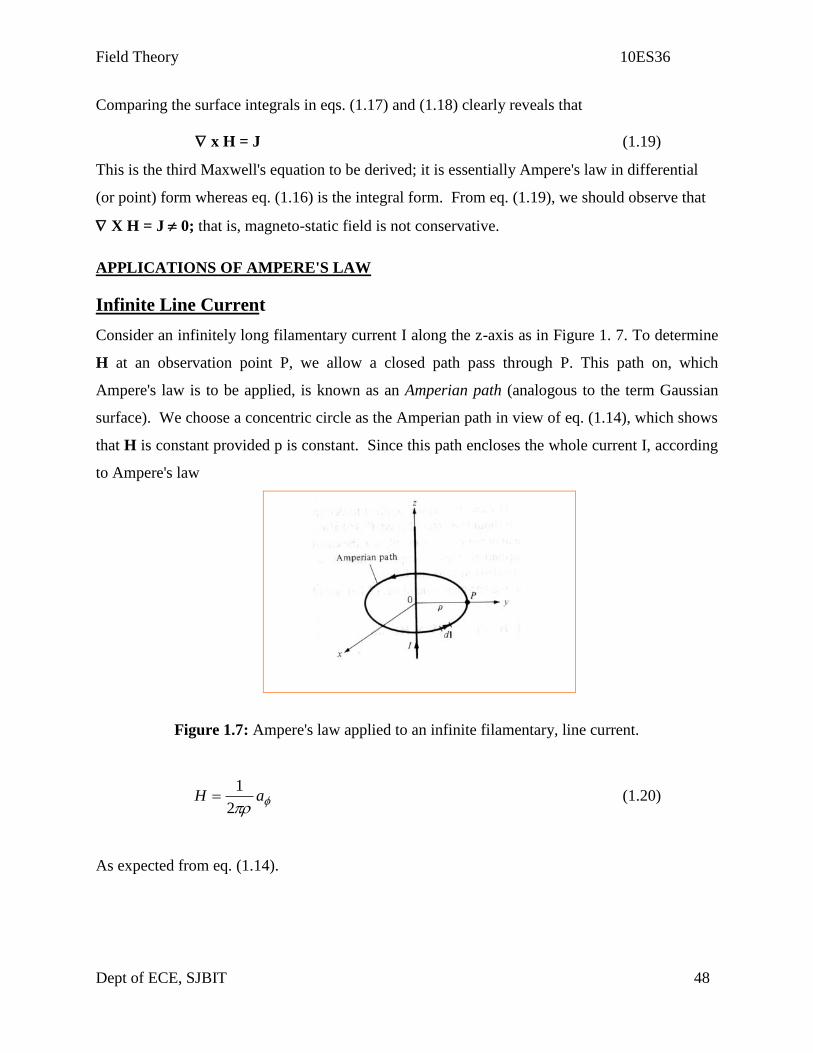
Consider an infinitely long filamentary current I along the z-axis as in Figure 1. 7. To determine

H at an observation point P, we allow a closed path pass through P. This path on, which

Ampere's law is to be applied, is known as an Amperian path (analogous to the term Gaussian

surface). We choose a concentric circle as the Amperian path in view of eq. (1.14), which shows

that H is constant provided p is constant. Since this path encloses the whole current I, according

to Ampere's law

Figure 1.7: Ampere's law applied to an infinite filamentary, line current.

aH2

1 (1.20)

As expected from eq. (1.14).

Field Theory 10ES36


MAGNETIC FLUX DENSITY

The magnetic flux density B is similar to the electric flux density D. As D = 0E in free space,

the magnetic flux density B is related to the magnetic field intensity H according to

B = 0 H (1.21)

where, 0 is a constant known as the permeability of free space. The constant is in henrys/meter

(H/m) and has the value of

0 = 4 x 10-7

H/m (1.22)

The precise definition of the magnetic field B, in terms of the magnetic force, can be discussed

later.

Figure 1.8: Magnetic flux lines due to a straight wire with current coming out of the page

The magnetic flux through a surface S is given by

S

dSB (1.23)

Where the magnetic flux is in webers (Wb) and the magnetic flux density is a webers/square

meter (Wb/m2) or teslas.

An isolated magnetic charge does not exit. Total flux through a closed surface in a magnetic

field must be zero;

that is,

0 dSB (1.24)

Field Theory 10ES36


This equation is referred to as the law of conservation of magnetic flux or Gauss'’s law for

magnetostatic fields just as D. dS = Q is Gauss's law for electrostatic fields. Although the

magnetostatic field is not conservative, magnetic flux is conserved.

By applying the divergence theorem to eq. (1.24), we obtain

0 Sv

dvBdSB

Or

. B = 0 (1.25)

This equation is the fourth Maxwell's equation to be derived. Equation (1.24) or (1.25) shows

that magnetostatic fields have no sources or sinks. Equation (1.25) suggests that magnetic field

lines are always continuous.

TABLE 1.2: Maxwell's Equations for Static EM Fields

Differential (or

Point) Form

Integral Form Remarks

. D = v S

v

vdvdSD Gauss's law

. B = 0 S

dSB 0 Nonexistence of magnetic monopole

x E = 0 L

dlE 0 Conservativeness of electrostatic field

x H = J L

s

dSJdlH Ampere's law

The Table 1.2 gives the information related to Maxwell's Equations for Static Electromagnetic

Fields.

MAGNETIC SCALAR AND VECTOR POTENTIALS

We recall that some electrostatic field problems were simplified by relating the electric Potential

V to the electric field intensity E (E = -V). Similarly, we can define a potential

Field Theory 10ES36


associated with magnetostatic field B. In fact, the magnetic potential could be scalar Vm vector

A. To define Vm and A involves two important identities:

x (V) = 0 (1.26)

. ( x A) = 0 (1.27)

which must always hold for any scalar field V and vector field A.

Just as E = -V, we define the magnetic scalar potential Vm (in amperes) as related to H

according to

H = - Vm if J = 0 (1.28)

The condition attached to this equation is important and will be explained. Combining eq. (1.28)

and eq. (1.19) gives

J = x H = - x (- Vm) = 0 (1.29)

since Vm, must satisfy the condition in eq. (1.26). Thus the magnetic scalar potential Vm is only

defined in a region where J = 0 as in eq. (1.28). We should also note that Vm satisfies Laplace's

equation just as V does for electrostatic fields; hence,

2 Vm = 0, (J = 0) (1.30)

We know that for a magnetostatic field, x B = 0 as stated in eq. (1.25). In order to satisfy eqs.

(1.25) and (1.27) simultaneously, we can define the vector magnetic potential A (in Wb/m) such

that

B = x A (1.31)

Just as we defined

r

dQV

04 (1.32)

We can define

L R

dlIA

4

0 for line current (1.33)

Field Theory 10ES36


S R

dSKA

4

0 for surface current (1.34)

v R

dvJA

4

0 for volume current (1.35)

Illustration 1: Given the magnetic vector potential A = -2/4 az Wb/m, calculate the total

magnetic flux crossing the surface = /2, 1 2m, 0 z 5m.

Solution:

adzddSaa

AAB z

,

2

4

15)5(

4

1

2

1 22

1

5

0

dzddSBz

= 3.75 Wb

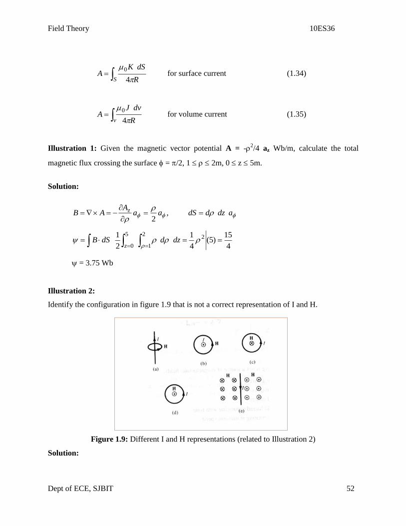
Illustration 2:

Identify the configuration in figure 1.9 that is not a correct representation of I and H.

Figure 1.9: Different I and H representations (related to Illustration 2)

Solution:

Field Theory 10ES36


Figure 1.9 (c) is not a correct representation. The direction of H field should have been outwards

for the given I direction.


1. State and prove Biot Savart’s law.

2. Derive for H at a point due to an infinite long conductor.

3. Derive for H at a point due to finite straight conductor.

4. Derive for H on the axis of a circular loop.

5. State and prove Ampere’s circuit law.

6. Mention the applications of Ampere’s circuit law and derive any one of them in brief.

7. Define curl and discuss the significance of curl.

8. Derive for Ampere’s law in point form.

9. Define magnetic flux & flux density.

10. Write a short note on magnetic scalar and vector potential.

Field Theory 10ES36


UNIT – 5

MAGNETIC FORCES, MATERIALS AND INDUCTANCE

Syllabus:

(a).Force on a moving charge and differential current element, Force between differential current

elements, Force and Torque on a closed circuit,

(b).Magnetic materials and inductance, Magnetization and permeability, Magnetic boundary

conditions, Magnetic circuits, Potential energy and forces on magnetic materials, Inductance and

mutual inductance

REFERENCE BOOKS:


edition,2006.


edition, 1999




2002



Force on a Charged Particle

According to earlier information, the electric force Fe, on a stationary or moving electric charge

Q in an electric field is given by Coulornb's experimental law and is related to the electric field

intensity E as

Fe = QE (2.1)

This shows that if Q is Positive, Fe and E have the same direction.

A magnetic field can exert force only on a moving charge. From experiments, it is found that the

magnetic force Fm experienced by a charge Q moving with a velocity u in a magnetic field B is

Fm = Qu x B (2.2)

This clearly shows that Fm is perpendicular to both u and B.

Field Theory 10ES36


From eqs. (2.1) and (2.2), a comparison between the electric force Fe and the magnetic force Fm

can be made. Fe is independent of the velocity of the charge and can perform work on the charge

and change its kinetic energy. Unlike Fe, Fm depends on the charge velocity and is normal to

it. Fm cannot perform work because it is at right angles to the direction of motion, of the charge

(Fm.dl = 0); it does not cause an increase in kinetic energy of the charge. The magnitude of Fm is

generally small compared to Fe except at high velocities.

For a moving charge Q in the Presence of both electric and magnetic fields, the total force on the

charge is given by

F = Fe + Fm

or

F = Q (E + u x B) (2.3)

This is known as the Lorentz force equation. It relates mechanical force to electrical force. If the

mass of the charged Particle moving in E and B fields is m, by Newton's second law of motion.

BuEQdt

dumF (2.4)

The solution to this equation is important in determining the motion of charged particles in E and

B fields. We should bear in mind that in such fields, energy transfer can be only by means of the

electric field. A summary on the force exerted on a charged particle is given in table 2.1.

TABLE 2.1: Force on a Charged Particle

State of Particle E Field B Field Combined E and B

Fields

Stationary QE - QE

Moving QE Qu x B Q(E + u x B)

The magnetic field B is defined as the force per unit current element

Alternatively, B may be defined from eq. (2.2) as the vector which satisfies Fm / q = u x B just as

we defined electric field E as the force per unit charge, Fe / q.

Field Theory 10ES36


Force between Two Current Elements

Let us now consider the force between two elements I1 dl1 and I2 dl2. According to Biot-Savart's

law, both current elements produce magnetic fields. So we may find the force d(dF1) on element

I1 dl1 due to the field dB2 produced by element I2 dl2 as shown in Figure 2.1.

As per equation

dF = I dl x B2

d(dF1) = I1 dl1 x dB2 (2.5)

But from Biot-Savart's law,

2

21

220

24

21

R

adlIdB

R

(2.6)

Hence,

2

21

22110

14

)( 21

R

adlIdlIdFd

R

(2.7)

Figure 2.1: Force between two current loops.

This equation is essentially the law of force between two current elements and is analogous to

Coulomb's law, which expresses the force between two stationary charges. From eq. (2.7), we

obtain the total force F1 on current loop 1 due to current loop 2 shown Figure 2.1 as

2 2

21

21210

121

14 L

R

L R

adldlIIF

(2.8)

Field Theory 10ES36


Although this equation appears complicated, we should remember that it is based on eq. (2.5). It

is eq. (8. 10) that is of fundamental importance.

The force F2 on loop 2 due to the magnetic field B1 from loop 1 is obtained from eq. (2.8) by

interchanging subscripts 1 and 2. It can be shown that F2 = - F1; thus F1 and F2 obey Newton's

third law that action and reaction are equal and opposite. It is worthwhile to mention that eq.

(2.8) was experimentally established by Qersted and Ampete; Biot and Savart (Ampere's

colleagues) actually based their law on it.

MAGNETIC TORQUE AND MOMENT

Now that we have considered the force on a current loop in a magnetic field, we can determine

the torque on it. The concept of a current loop experiencing a torque in a magnetic field is of

paramount importance in understanding the behavior of orbiting charged particles, d.c. motors,

and generators. If the loop is placed parallel to a magnetic field, it experiences a force that tends

to rotate it.

The torque T (or mechanical moment of force) on the loop is the, vector product of the force F

and the moment arm r.

That is,

T = r x F (2.9)

and its units are Newton-meters.

Let us apply this to a rectangular loop of length l and width w placed in a uniform magnetic field

B as shown in Figure 8.5(a). From this figure, we notice that dl is parallel to B along sides 12

and 34 of the loop and no force is exerted on those sides. Thus

3

2

1

4BdlIBdlIF

l

lzz BadzIBadzI

2

0

Field Theory 10ES36


Figure 2.2: Rectangular planar loop in a uniform magnetic field.

or

F= F0 – F0 = 0 (2.10)

Where, |F0| = I Bl because B is uniform. Thus, no force is exerted on the loop as a whole.

However, F0 and –F0 act at different points on the loop, thereby creating a couple. If the normal

to the plane of the loop makes an angle with B, as shown in the cross-sectional view of Figure

2.2(b), the torque on the loop is

|T| = |F0| w sin

or

T = B I l w sin (2.11)

But lw = S, the area of the loop. Hence,

T = BIS sin (2.12)

We define the quantity

m = I S an (2.13)

as the magnetic dipole moment (in A/M2) of the loop. In eq. (2.13), an is a unit normal vector to

the plane of the loop and its direction is determined by the right-hand rule: fingers in the

direction of current Hand thumb along an.

The magnetic dipole moment is the product of current and area of the loop; its reaction is normal

to the loop.

Introducing eq. (2.13) in eq. (2.12), we obtain

Field Theory 10ES36


T = m x B (2.14)

Stoke's theorem

Stoke's Theorem relates a line integral to the surface integral and vice-versa, that is

C

S

dSHdLH )( (3.1)

Force on a moving charge due to electric and magnetic fields

If there is a charge or a moving charge, Q in an electric field, E, there exists a force on the

charge. This force is given by

FE = QE (3.2)

If a charge, Q moving with a velocity, V is placed in a magnetic field, B (=H), then there exists

a force on the charge (Fig. 3.1). This force is given by

FH = Q(V x B) (3.3)

B = magnetic flux density, (wb/m2)

V = velocity of the charge, m/s

Fig. 3.1: Direction of field, velocity and force

If the charge, Q is placed in both electric and magnetic fields, then the force on the charge is

F =Q (E + V x B) (3.4)

This equation is known as Lorentz force equation.

Field Theory 10ES36


Problem 1: A charge of 12 C has velocity of 5ax + 2ay - 3az m/s. Determine F on the charge in

the field of (a) E=18ax,+5ay +10az V/m

(b) B = 4ax + 4ay + 3az wb/m2.

Solution:

(a) The force, F on the charge, Q due to E is

F = QE = 12 (18ax + 5ay + 10az)

= 216ax + 60ay + 120az

or, F=Q |E|=222 1051812

F = 254.27 N

(b) The force F on the charge due to B is

F = Q[V x B)

Here V = 5ax + 2ay - 3az m/s

B = 4 ax + 4 ay + 3 az wb / m2

F = 12 [18ax - 27ay + 12az]

or, F= )144729324(12

F = 415.17 N

Force on a current element in a magnetic field

The force on a current element when placed in a magnetic field, B is

F = IL x B (3.5)

or,

F = I L B Sin Newton (3.6)

where is the angle between the direction of the current element and the direction of magnetic

flux density

B = magnetic flux density, wb/m2

IL = current element, Amp-m

Proof: Consider a differential charge, dQ to be moving with a velocity, V in a magnetic field, H

= (B/). Then the differential force on the charge is given by

Field Theory 10ES36


dF = dQ (V x B) (3.7)

But

dQ = d

dF = d (V x B)

= ( V x B) d

But V = J

dF = J d x B

Jd is nothing but IdL,

dF =IdL x B

or, F = IL x B, Newton (3.8)

Problem 2: A current element 4 cm long is along y-axis with a current of 10 mA flowing in y-

direction. Determine the force on the current element due to the magnetic field if the magnetic

field H = (5ax/) A/m.

Solution:

The force on a current element under the influence of magnetic field is

F = IL x B

Here, IL = 10 x 10-3

x 0.04ay

= 4 x l0-4

ay

H = (5ax/) A/m

B = 5ax wb/m2

F = 4 x l0-4

ay x 5ax

or F = (0.4ay x 5ax) x 10-3

F = -2.0az mN

Field Theory 10ES36


BOUNDARY CONDITIONS ON H AND B

1. The tangential component of magnetic field, H is continuous across any boundary except

at the surface of a perfect conductor, that is,

Htanl - Htan2 = Js (3.9)

At non-conducting boundaries, Js = 0.

2. The normal component of magnetic flux density, B is continuous across any

discontinuity, that is,

Bnl = Bn2 (3.10)

Proof: Consider Fig. 3.2 in which a differential rectangular loop across a boundary separating

medium 1 and medium 2 are shown.

Fig. 3.2: A rectangular loop across a boundary

From Ampere's circuit law, we have

453423120150

dLH

113422

yxyy HxHy

Hy

H

IxHy

Hy

xy

2222

Field Theory 10ES36


As y 0, we get

IxHxHdLH xx 21

or,

sxx Jx

IHH

21

(3.11)

Here, Hxl and Hx2 are tangential components in medium 1 and 2, respectively.

So, Htan1 – Htan2 = Js (3.12)

Now consider a cylinder shown in Fig. 3.3.

Fig. 3.3: A differential cylinder across the boundary

Gauss's law for magnetic fields is

s

dSB 0 (3.13)

In this case, for y 0

s

yy

s

nyy

s

n adSaBadSaBdSB )(21 (3.14)

that is, Bn1 S - Bn2 S = 0

Therefore, Bnl = Bn2 (3.15)

Field Theory 10ES36


Problem 3:

Two homogeneous, linear and isotropic media have an interface at x = 0. x < 0 describes

medium 1 and x > 0 describes medium 2. r1 = 2 and r2 = 5. The magnetic field in medium 1

is 150ax - 400ay + 250az A/m.

Determine:

(a) Magnetic field in medium 2

(b) Magnetic flux density in medium 1

(c) Magnetic flux density in medium 2.

Solution:

The magnetic field in medium 1 is

H1 = 150ax - 400ay +250az A/m

Consider Fig. 3.4.

Fig. 3.4: Illustrative figure

(a) H1 = Htan1 + Hn1

Htanl = -400ay + 250az A/m

Hn1 = 150ax

The boundary condition is

Htanl = Htan2

Htan2 = - 400ay + 50az A/m

The boundary condition on B is Bn1 = Bn2

that is, 1 Hn1 = 1 Hn2

1

2

12 nn HH

xa150

5

2 = 60ax

H2 = Htan2 + Hn2

Field Theory 10ES36


(b) B1= 1 H1

= 0 r H1

=4 x 10-7

x 2(150ax - 400ay + 250az)

= (376.5ax - 1004ay + 627.5az) wb/m2

(c) B2 = 2 H2

= 4 x 10-7

x 5 (60ax - 400ay + 250az)

= (376.98ax - 2513.2ay +1570.75az)wb/m2

SCALAR MAGNETIC POTENTIAL

Like scalar electrostatic potential, it is possible to have scalar magnetic potential. It is defined in

such a way that its negative gradient gives the magnetic field, that is,

H = Vm (3.16)

Vm = scalar magnetic potential (Amp)

Taking curl on both sides, we get

x H = - x Vm (3.17)

But curl of the gradient of any scalar is always zero.

So, x H =0 (3.18)

But, by Ampere's circuit law X H = J

or, J = 0

In other words, scalar magnetic potential exists in a region where J = 0.

H = -Vm (J=0) (3.19)

The scalar potential satisfies Laplace's equation, that is, we have

.B = 0 .H = 0 = m (-Vm) = 0

or,

2 Vm = 0 (J = 0) (3.20)

Field Theory 10ES36


Characteristics of Scalar Magnetic Potential (Vm)

1. The negative gradient of Vm gives H, or H = -Vm

2. It exists where J = 0

3. It satisfies Laplac’s equation.

4. It is directly defined as

B

A

m dLHV

5. It has the unit of Ampere.

VECTOR MAGNETIC POTENTIAL

Vector magnetic potential exists in regions where J is present. It is defined in such a way that

its curl gives the magnetic flux density, that is,

B x A (3.21)

where A = vector magnetic potential (wb/m).

It is also defined as

m

AmpHenry

R

IdLA

4

0 (3.22)

or, ,4

0

s

R

KdsA

(K = current sheet) (3.23)

or, ,4

0

v

R

JdvA

(3.24)

Field Theory 10ES36


Characteristics of Vector Magnetic Potential

1. It exists even when J is present.

2. It is defined in two ways

B x A and

v

R

Jd

4

0

3. 2A = 0 j

4. 2A = 0 if J = 0

5. Vector magnetic potential, A has applications to obtain radiation characteristics of

antennas, apertures and also to obtain radiation leakage from transmission lines,

waveguides and microwave ovens.

6. A is used to find near and far-fields of antennas.

Problem 4:

The vector magnetic potential, A due to a direct current in a conductor in free space is given by

A = (X2 + Y

2) az wb /m

2. Determine the magnetic field produced by the current element at (1,

2, 3).

Solution:

A = (x2 +y

2) az wb/m

2

We have B = x A

22

6

00

10

yx

zyx

aaa zyx

62222 10

yx ayx

xayx

x

Field Theory 10ES36


622 1022 yx ayxayx

6104241)3,2,1(/ yx aaatB

61065 yx aa

6

0

10651 yx aaH

6

71065

104

1

yx aa

H = (3.978ax – 4.774ay), A/m

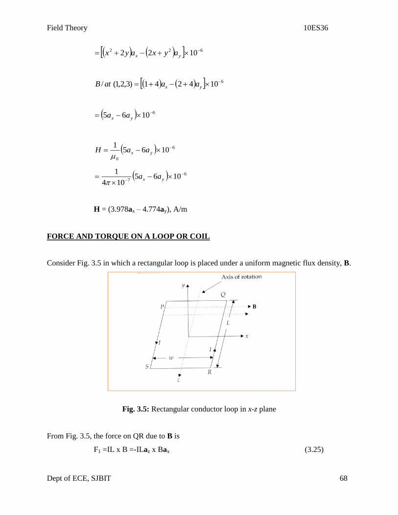
FORCE AND TORQUE ON A LOOP OR COIL

Consider Fig. 3.5 in which a rectangular loop is placed under a uniform magnetic flux density, B.

Fig. 3.5: Rectangular conductor loop in x-z plane

From Fig. 3.5, the force on QR due to B is

F1 =IL x B =-ILaz x Bax (3.25)

Field Theory 10ES36


F1 = -ILBay (3.26)

that is, the force, F1 on QR moves it downwards. Now the force on PS is

F2 = IL x B = -ILaz x Bax (3.27)

F2 = - ILBay (3.28)

Force, F2 on PS moves it upwards. It may be noted that the sides PQ and

SR will not experience force as they are parallel to the field, B.

The forces on QR and PS exert a torque. This torque tends to rotate the coil about its axis.

The torque, T is nothing but a mechanical moment of force. The torque on the loop is defined as

the vector product of moment arm and force,

that is,

T r x F, N-m (3.29)

where r = moment arm

F = force

Applying this definition to the loop considered above, the expression for

torque is given by

T = r1 x F1 + r2 x F2 (3.30)

)(2

)(2

yxyx ILBaaw

ILBaaw

(3.31)

= -BILwaz

or, T = -BISaz (3.32)

where S = wL = area of the loop

Field Theory 10ES36


The torque in terms of magnetic dipole moment, m is

T = m x B, N-m (3.34)

where m = I l w ay

= I S ay

Problem 5:

A rectangular coil is placed in a field of B = (2ax + ay) wb/m2. The coil is in y-z plane and has

dimensions of 2 m x 2 m. It carries a current of 1 A. Find the torque about the z-axis.

Solution:

m=IS an = 1 x 4ax

T = m x B = 4ax x (2ax + ay)

T = 4az, N-m

MATERIALS IN MAGNETIC FIELDS

A material, is said to be magnetic if m 0, r = 1

A material is said to be non-magnetic if m = 0, r = 1.

The term 'Magnetism' is commonly discussed in terms of magnets with basic examples like north

pole, compass needle, horse shoe magnets and so on.

Magnetic properties are described in terms of magnetic susceptibility and relative permeability of

the materials.

Field Theory 10ES36


Magnetic materials are classified into

1. Diamagnetic materials

2. Paramagnetic materials

3. Ferromagnetic materials

Diamagnetic Materials

A material is said to diamagnetic if its susceptibility, m < 0 and r 1.0.

Examples are copper, lead, silicon, diamond and bismuth.

Characteristics of diamagnetic materials

Magnetic fields due to the motion of orbiting electrons and spinning electrons cancel

each other.

Permanent magnetic moment of each atom is zero.

These materials are widely affected by magnetic field.

Magnetic susceptibility m is (-)ve.

r = 1

B = 0

Most of the materials exhibit diamagnetism.

They are linear magnetic materials.

Diamagnetism is not temperature dependent.

These materials acquire magnetisation opposite to H and hence they are called

diamagnetic materials.

Paramagnetic Materials

A material for which m > 0 and r 1 is said to be paramagnetic.

Examples are air, tungsten, potassium and platinum.

Field Theory 10ES36


Characteristics of paramagnetic materials

They have non-zero permanent magnetic moment.

Magnetic fields due to orbiting and spinning electrons do not cancel each other.

Paramagnetism is temperature dependent.

m lies between 10-5

and 10-3

.

These are used in MASERS.

m > 0

r 1

They are linear magnetic materials.

These materials acquire magnetisation parallel to H and hence they are called paramagnetic

materials.

Ferromagnetic Materials

A material for which m >> 0, r >> 1 is said to be ferromagnetic.

Examples are iron, nickel, cobalt and their alloys.

Characteristics of ferromagnetic materials

They exhibit large permanent dipole moment.

m >> 0

r >> l

They are strongly magnetised by magnetic field.

They retain magnetism even if the magnetic field is removed.

They lose their ferromagnetic properties when the temperature is raised.

If a permanent magnet made of iron is heated above its curie temperature, 770C, it loses

its magnetisation completely.

They are non-linear magnetic materials.

B = H does not hold good as depends on B.

Field Theory 10ES36


In these materials, magnetisation is not determined by the field present. It depends on the

magnetic history of the object.

INDUCTANCE

Inductor is a coil of wire wound according to various designs with or without a core of magnetic

material to concentrate the magnetic field.

Inductance, L In a conductor, device or circuit, an inductance is the inertial property caused by

an induced reverse voltage that opposes the flow of current when a voltage is applied. It also

opposes a sudden change in current that has been established.

Definition of Inductance, L (Henry):

The inductance, L of a conductor system is defined as the ratio of magnetic flux linkage to the

current producing the flux, that is,

)(HenryI

NL

(3.35)

Here N = number of turns

= flux produced

I = current in the coil

1 Henry l wb/Amp

L is also defined as (2WH/I2), or

2

2

I

WL H (3.36)

where, WH = energy in H produced by I.

In fact, a straight conductor carrying current has the property of inductance. Aircore coils are

wound to provide a few pico henries to a few micro henries. These are used at IF and RF

frequencies in tuning coils, interstage coupling coils and so on.

Field Theory 10ES36


The requirements of such coils are:

Stability of inductance under all operating conditions

High ratio inductive reactance to effective loss resistance at the operating freq

Low self capacitance

Small size and low cost

Low temperature coefficient

STANDARD INDUCTANCE CONFIGURATIONS

Toroid

It consists of a coil wound on annular core. One side of each turn of the coil is threaded through

the ring to form a Toroid (Fig. 3.6).

Fig. 3.6: Toroid

Inductance of Toroid, r

SNL

2

2

0 (3.37)

Here N = number of turns

r = average radius

S = cross-sectional area

Magnetic field in a Toroid, r

NIH

2 (3.38)

I is the current in the coil.

Field Theory 10ES36


Solenoid

It is a coil of wire which has a long axial length relative to its diameter. The coil is tubular in

form. It is used to produce a known magnetic flux density along its axis.

A solenoid is also used to demonstrate electromagnetic induction. A bar of iron, which is free to

move along the axis of the coil, is usually provided for this purpose. A typical solenoid is shown

in Fig. 3.7.

Fig. 3.7: Solenoid

The inductance, L of a solenoid is

l

SNL

2

0 (3.39)

l = length of solenoid

S = cross-sectional area

N = Number of turns

The magnetic field in a solenoid is

l

NIH (3.40)

I is the current

Field Theory 10ES36



1. Derive for force on a moving charge.

2. Derive for Lorentz force equation.

3. Derive for force between differential current elements.

4. Derive for force & torque on a closed circuit.

5. Discuss briefly about magnetic materials.

6. Discuss briefly about magnetic boundary conditions.

Field Theory 10ES36


UNIT – 6

TIME VARYING MAGNETIC FIELDS AND MAXWELLS EQUATIONS

Syllabus:

Faraday’s law, Displacement current, Maxwell’s equation in point and integral form, Retarded

potentials.

REFERENCE BOOKS:


edition,2006.


edition, 1999




2002



Introduction

Electrostatic fields are usually produced by static electric charges whereas magnetostatic fields

are due to motion of electric charges with uniform velocity (direct current) or static magnetic

charges (magnetic poles); time-varying fields or waves are usually due to accelerated charges or

time-varying current.

Stationary charges Electrostatic fields

Steady current Magnetostatic fields

Time-varying current Electromagnetic fields (or waves)

Faraday discovered that the induced emf, Vemf (in volts), in any closed circuit is equal to the time

rate of change of the magnetic flux linkage by the circuit

Field Theory 10ES36


This is called Faraday’s Law, and it can be expressed as

dt

dN

dt

dVemf

1.1

where N is the number of turns in the circuit and is the flux through each turn. The negative

sign shows that the induced voltage acts in such a way as to oppose the flux producing it. This is

known as Lenz’s Law, and it emphasizes the fact that the direction of current flow in the circuit

is such that the induced magnetic filed produced by the induced current will oppose the original

magnetic field.

Fig. 1 A circuit showing emf-producing field Ef and electrostatic field Ee

TRANSFORMER AND MOTIONAL EMFS

Having considered the connection between emf and electric field, we may examine how

Faraday's law links electric and magnetic fields. For a circuit with a single (N = 1), eq. (1.1)

becomes

dt

dNVemf

1.2

In terms of E and B, eq. (1.2) can be written as

SL

emf dSBdt

ddlEV 1.3

where, has been replaced by S

dSB and S is the surface area of the circuit bounded by the

closed path L. It is clear from eq. (1.3) that in a time-varying situation, both electric and

magnetic fields are present and are interrelated. Note that dl and dS in eq. (1.3) are in accordance

with the right-hand rule as well as Stokes's theorem. This should be observed in

Field Theory 10ES36


Figure 2. The variation of flux with time as in eq. (1.1) or eq. (1.3) may be caused in three ways:

1. By having a stationary loop in a time-varying B field

2. By having a time-varying loop area in a static B field

3. By having a time-varying loop area in a time-varying B field.

A. STATIONARY LOOP IN TIME-VARYING B FIELD (TRANSFORMER EMF)

This is the case portrayed in Figure 2 where a stationary conducting loop is in a time varying

magnetic B field. Equation (1.3) becomes

SL

emf dSt

BdlEV 1.4

Fig. 2: Induced emf due to a stationary loop in a time varying B field.

This emf induced by the time-varying current (producing the time-varying B field) in a stationary

loop is often referred to as transformer emf in power analysis since it is due to transformer

action. By applying Stokes's theorem to the middle term in eq. (1.4), we obtain

SS

dSt

BdSE 1.5

For the two integrals to be equal, their integrands must be equal; that is,

t

BE

1.6

Field Theory 10ES36


This is one of the Maxwell's equations for time-varying fields. It shows that the time varying E

field is not conservative ( x E 0). This does not imply that the principles of energy

conservation are violated. The work done in taking a charge about a closed path in a time-

varying electric field, for example, is due to the energy from the time-varying magnetic field.

B. MOVING LOOP IN STATIC B FIELD (MOTIONAL EMF)

When a conducting loop is moving in a static B field, an emf is induced in the loop. We recall

from eq. (1.7) that the force on a charge moving with uniform velocity u in a magnetic field B is

Fm = Qu x B 1.7

We define the motional electric field Em as

BuQ

FE m

m 1.8

If we consider a conducting loop, moving with uniform velocity u as consisting of a large

number of free electrons, the emf induced in the loop is

LL

memf dlBudlEV 1.9

This type of emf is called motional emf or flux-cutting emf because it is due to motional action.

It is the kind of emf found in electrical machines such as motors, generators, and alternators.

C. MOVING LOOP IN TIME-VARYING FIELD

This is the general case in which a moving conducting loop is in a time-varying magnetic field.

Both transformer emf and motional emf are present. Combining equation 1.4 and 1.9 gives the

total emf as

LL S

emf dlBudSt

BdlEV 1.10

BuEm 1.11

or from equations 1.6 and 1.11.

But

BE

1.12

Field Theory 10ES36


DISPLACEMENT CURRENT

For static EM fields, we recall that

x H = J 1.13

But the divergence of the curl of any vector field is identically zero.

Hence,

. ( x H) = 0 = . J 1.14

The continuity of current requires that

0

tJ v 1.15

Thus eqs. 1.14 and 1.15 are obviously incompatible for time-varying conditions. We must

modify eq. 1.13 to agree with eq. 1.15. To do this, we add a term to eq. 1.13, so that it becomes

x H = J + Jd 1.16

where Jd is to be determined and defined. Again, the divergence of the curl of any vector is zero.

Hence:

. ( x H) = 0 = . J + . Jd 1.17

In order for eq. 1.17 to agree with eq. 1.15,

t

DD

ttJJ v

d

1.18

or

t

DJ d

1.19

Substituting eq. 1.19 into eq. 1.15 results in

t

DJH

1.20

This is Maxwell's equation (based on Ampere's circuit law) for a time-varying field. The term Jd

= D/t is known as displacement current density and J is the conduction current density (J =

E)3.

Field Theory 10ES36


Fig. 3 Two surfaces of integration showing the need for Jd in Ampere’s circuit law

The insertion of Jd into eq. 1.13 was one of the major contribution of Maxwell. Without the term

Jd, electromagnetic wave propagation (radio or TV waves, for example) would be impossible. At

low frequencies, Jd is usually neglected compared with J. however, at radio frequencies, the two

terms are comparable. At the time of Maxwell, high-frequency sources were not available and

eq. 1.20 could not be verified experimentally.

Based on displacement current density, we define the displacement current as

dS

t

DdSJI dd 1.21

We must bear in mind that displacement current is a result of time-varying electric field. A

typical example of such current is that through a capacitor when an alternating voltage source is

applied to its plates.

PROBLEM: A parallel-plate capacitor with plate area of 5 cm2 and plate separation of 3 mm

has a voltage 50 sin 103 t V applied to its plates. Calculate the displacement current assuming =

2 0.

Solution:

d

VED

dt

dV

dt

DJ d

Hence,

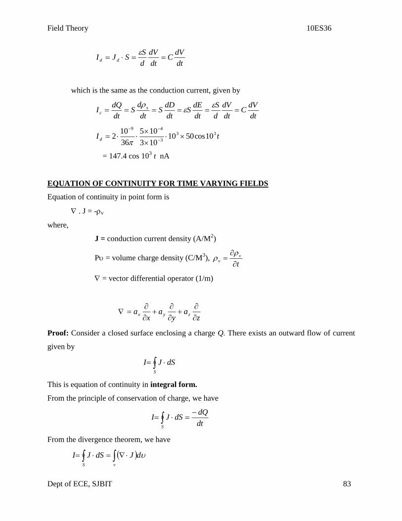
Field Theory 10ES36


dt

dVC

dt

dV

d

SSJI dd

which is the same as the conduction current, given by

dt

dVC

dt

dV

d

S

dt

dES

dt

dDS

dt

dS

dt

dQI s

c

tI d

33

3

49

10cos5010103

105

36

102

= 147.4 cos 103 t nA

EQUATION OF CONTINUITY FOR TIME VARYING FIELDS

Equation of continuity in point form is

. J = -v

where,

J = conduction current density (A/M2)

P = volume charge density (C/M3),

t

v

v

= vector differential operator (1/m)

z

ay

ax

a zyx

Proof: Consider a closed surface enclosing a charge Q. There exists an outward flow of current

given by

S

dSJI

This is equation of continuity in integral form.

From the principle of conservation of charge, we have

dt

dQdSJI

S

From the divergence theorem, we have

vS

dJdSJI

Field Theory 10ES36


Thus, dt

dQdJ

By definition,

dQ

where , = volume charge density (C/m3)

So,

ddt

dJ.

where t

.

The volume integrals are equal only if their integrands are equal.

Thus, . J = - .

MAXWELL'S EQUATIONS FOR STATIC EM FIELDS

Differential (or

Point) Form Integral Form Remarks

. D = v S

v

vdvdSD Gauss's law

. B = 0 S

dSB 0 Nonexistence of magnetic

monopole

x E =-t

B

Ls

dSBt

dlE Faraday’s Law

x H = J + t

D

Ls

dSJdlH Ampere's circuit law

MAXWELL’S EQUATIONS FOR TIME VARYING FIELDS

These are basically four in number.

Maxwell's equations in differential form are given by

x H = t

D

+ J

Field Theory 10ES36


x E = -t

B

.D =

.B = 0

Here,

H = magnetic field strength (A/m)

D = electric flux density, (C/m2)

(D/t) = displacement electric current density (A/m2)

J = conduction current density (A/m 2

)

E = electric field (V/m)

B = magnetic flux density wb/m2 or Tesla

(B/t) = time-derivative of magnetic flux density (wb/m2 -sec)

B is called magnetic current density (V/m2) or Tesla/sec

P = volume charge density (C/m3)

Maxwell's equations for time varying fields in integral form are given by

L S

dSJDdLH.

L S

dSBdLE

S

ddSD

S

dSB 0

DEFINITIONS OF MAXWELL'S EQUATIONS

1. The first Maxwell's equation states that the magnetomotive force around a closed path is

equal to the sum of electric displacement and, conduction currents through any surface

bounded by the path.

2. The second law states that the electromotive force around a closed path is equal to the

inflow of magnetic current through any surface bounded by the path.

3. The third law states that the total electric displacement flux passing through a closed

surface (Gaussian surface) is equal to the total charge inside the surface.

Field Theory 10ES36


4. The fourth law states that the total magnetic flux passing through any closed surface is

zero.

MAXWELL’S EQUATIONS FOR STATIC FIELDS

Maxwell’s Equations for static fields are:

SL

dSJdLHJH

00 L

dLEE

ddSDDS

00 S

dSBB

As the fields are static, all the field terms which have time derivatives are zero, that is, t

D

= 0,

t

B

= 0.

PROOF OF MAXWELLS EQUATIONS

1. From Ampere's circuital law, we have

x H = J

Take dot product on both sides

. x H = . J

As the divergence of curl of a vector is zero,

RHS = . J = 0

But the equation of continuity in point form is

tJ

This means that if x H = J is true, it is resulting in . J = 0.

As the equation of continuity is more fundamental, Ampere's circuital law

should be modified. Hence we can write

Field Theory 10ES36


x H = J + F

Take dot product on both sides

. x H = . J + . F

that is, . x H = 0 = . J + . F

Substituting the value of .J from the equation of continuity in the above

expression, we get

. F + (-) = 0

or, . F = -

The point form of Gauss's law is

. D =

or, . D =

From the above expressions, we get

. F = . D

The divergence of two vectors are equal only if the vectors are identical,

that is, F = D

So, x H = D + J

Hence proved.

2. According to Faraday's law,

dt

demf

= magnetic flux, (wb)

and by definition,

L

dLEemf

dt

ddLE

L

But S

dSB

SL

dSt

BdLE

Field Theory 10ES36


St

BBdSB ,

Applying Stoke's theorem to LHS, we get

SL

dSEdLE

S S

dSBdSE

Two surface integrals are equal only if their integrands are equal,

that is, x E = - B

Hence proved.

3. From Gauss's law in electric field, we have

dQdSDS

Applying divergence theorem to LHS, we get

ddDdSDS

Two volume integrals are equal if their integrands are equal,

that is, . D =

Hence proved.

4. We have Gauss's law for magnetic fields as

S

dSB 0

RHS is zero as there are no isolated magnetic charges and the magnetic flux lines are closed

loops.

Applying divergence theorem to LHS, we get

0dB

or,

. B = 0 Hence proved.

PROBLEM 1:

Given E = 10 sin (t - y) ay V/m, in free space, determine D, B and H.

Field Theory 10ES36


Solution:

E = 10 sin (t - y) ay, V/m

D = 0 E, 0 = 8.854 x 10-12

F/m

D = 100 sin (t - y) ay, C/m2

Second Maxwell’s equation is

x E = -B

That is,

00 y

zyx

E

zyx

aaa

E

or,

yzyx E

xaE

zaE 0

As Ey = 10 sin (t - z) V/m

0

x

E y

Now, x E becomes

x

ya

z

EE

= 10 cos (t - z) ax

t

B

xadtztB cos10

or 2/,sin10

mwbaztB z

and mAaztB

H z /,sin10

00

Field Theory 10ES36


PROBLEM 2: If the electric field strength, E of an electromagnetic wave in free space is given

by E = 2 cos ya

zt

0 V/m, find the magnetic field, H.

Solution: We have

B/t = - x E

00 y

zyx

E

zyx

aaa

yzyyx E

xaaE

za )0(

x

ya

z

E

xaz

t

00

sin2

xadt

ztB

00

sin2

or, xaz

tB

00

cos2

or, xaz

tB

H

0000

cos2

120

0

00

Thus, xaz

tH

00

cos2

00

0

1

mAaz

tH x /cos60

1

0

PROBLEM 3: If the electric field strength of a radio broadcast signal at a TV receiver is given

by

E = 5.0 cos (t - y) az, V/m,

Field Theory 10ES36


determine the displacement current density. If the same field exists in a medium whose

conductivity is given by 2.0 x 103 (mho)/cm, find the conduction current density.

Solution:

E at a TV receiver in free space

= 5.0 cos (t - y) az, V/m

Electric flux density

D = 0 E = 5 0 cos (t - y) az, V/m

The displacement current density

t

DDJ d

zaytt

cos5 0

Jd = -50 sin (t - y) az, V/m2

The conduction current density,

Jc = E

= 2.0 x 103 (mho) /cm

= 2 x 105 mho /m

Jc = 2 x 105 x 5 cos (t - y) az

Jc = 106 cos (t - y) az V/m

2


1. From faraday’s law, show that EMF= -N dΦ/dt

2. Derive for displacement current.

3. Prove that displacement current is equal to conduction current.

4. Write Maxwell’s equation in point form.

5. Write Maxwell’s equation in integral form.

Field Theory 10ES36


UNIT – 7

UNIFORM PLANE WAVES

Syllabus:

Wave propagation in free space and dielectrics, Poynting’s theorem and wave power,

Propagation in good conductors – (skin effect)

REFERENCE BOOKS:


edition,2006.


edition, 1999




2002



Sinusoidal Time Variations:

In practice, most generators produce voltage and currents and hence electric and magnetic

fields which vary sinusoidally with time. Further, any periodic variation can be represented

as a weight sum of fundamental and harmonic frequencies.

Therefore we consider fields having sinusoidal time variations, for example,

E = Em cos t

E = Em sin t

Here, w = 2f, f = frequency of the variation.

Therefore every field or field component varies sinusoidally, mathematically by an additional

term. Representing sinusoidal variation. For example, the electric field Er

can be represented

as

, , ,

., , ; , ,

E x y z t as

ie E r t r x y z

r

r r r%

Field Theory 10ES36


Where Er%

is the time varying field.

The time varying electric field can be equivalently represented, in terms of corresponding

phasor quantity Er%

(r) as

, ________ (11)j t

eE r t R E r e

r rr%

The symbol ‘tilda’ placed above the E vector represents that Er

is time – varying quantity.

The phasor notation:

We consider only one component at a time, say Ex.

The phasor Ex is defined by

, ________ (12)j t

x e xE r t R E r e r%

xE rr

denotes Ex as a function of space (x,y,z). In general xE rr

is complex and hence can be

represented as a point in a complex and hence can be represented as a point in a complex plane.

(see fig) Multiplication by jwte results in a rotation through an angle wt measured from the angle

. At t increases, the point Ex jwte traces out a circle with center at the origin. Its projection on

the real axis varies sinusoidally with time & we get the time-harmonically varying electric field

Ex% (varying sinusoidally with time). We note that the phase of the sinusoid is determined by ,

the argument of the complex number Ex.

Therefore the time varying quantity may be expressed as

________ (13)

cos( ) ________ (14)

j j t

x e x

x

E R E e e

E t

%

Field Theory 10ES36


Maxwell’s eqn. in phasor notation:

In time – harmonic form, the Maxwell’s first curl eqn. is:

_______ (15)D

H Jt

r%r r% %

using phasor notation, this eqn. becomes,

________ (16)j t j t j t

e e eR He R De R Jet

r r r

The diff. Operator & Re part operator may be interchanged to get,

0

j t j t j t

e e e

j t j t

e e

j t

e

R He R De R Jet

R j D e R Je

R H j D J e

r r r

r r

r r r

This relation is valid for all t. Thus we get

________ (17)H J j D r r r

This phasor form can be obtained from time-varying form by replacing each time derivative by

.,jw ie is to be replaced byt

For the sinusoidal time variations, the Maxwell’s equation may be expressed in phasor form as:

(17)

(18)

(19)

(20) 0 0

LS

LS

V VS

V

S

H J j D H dL J j D ds

E j B E dl j B ds

D D ds d

B B ds

r r r r r r rg g

rr r r r rg g

r r rg g

r r rg g

Ñ

Ñ

Ñ

Ñ

The continuity eqn., contained within these is,

_______ (21)S

vol

J j J ds j dv r r r

g gÑ

Field Theory 10ES36


The constitutive eqn. retain their forms:

D E

B H

J E

r r

r r

r r____ (22)

For sinusoidal time variations, the wave equations become

2 2

2 2

( )

( )

E E for electric field

H H for electric field

r r

r r _________ (23)

Vector Helmholtz eqn.

In a conducting medium, these become

2 2

2 2

0

0

E j E

H j H

r r

r r ________ (24)

Wave propagation in a loss less medium:

In phasor form, the wave eqn. for VPW is

222

22

2

2

1 2

; _______ (25)

_______ (26)

y

y

j x j x

y

EEE

Exx

E

E C e C e

rr

r

C1 & C2 are arbitrary constants.

The corresponding time varying field is

1 2

1 2

,

______ (27)

cos cos ______ (28)

j t

y e y

t z t zj j

e

E x t R E x e

R C e C e

C t z C t z

%

When C1 and C2 are real.

Therefore we note that, in a homogeneous, lossless medium, the assumption of sinusoidal time

variations results in a space variation which is also sinusoidal.

Eqn. (27) and (28) represent sum of two waves traveling in opposite directions.

Field Theory 10ES36


If C1 = C2 , the two traveling waves combine to form a simple standing wave which does not

progress.

If we rewrite eqn. (28) with Ey as a fn of (x-t),

we get =

Let us identify some point in the waveform and observe its velocity; this point is

t x a constant

Then

' 'a t

dx x

dt t

Q

This velocity is called phase velocity, the velocity of a phase point in the wave.

is called the phase shift constant of the wave.

Field Theory 10ES36


Wavelength: These distance over which the sinusoidal waveform passes through a full cycle of

2 radians

ie.,

0

2

2 2

2

;

1:

Z

or

But

f

or

f f in H

Wave propagation in a conducting medium

We have,

Where

2 2

2 2

0E E

j

j j

r r

is called the propagation constant is, in general, complex.

Therefore, = + j

= Attenuation constant

= phase shift constant.

The eqn. for UPW of electric field strength is

2

2

2

EE

x

rr

One possible solution is

0

xE x E e r

Therefore in time varying form, we get

Field Theory 10ES36


0

, x j t

e

x jwt

e

E x t R E e e

e R E e

r%

This eqn. shown that a up wave traveling in the +x direction and attenuated by a factor xe .

The phase shift factor

2

and velocity f

= Real part of = RP j j t

=

2

2 2

2

2 2

1 12

1 12

Conductors and dielectrics:

We have the phasor form of the 1st Maxwell’s curl eqn.

c dispH E j E J J r r r

where cJ E r

conduction current density ( A/m2 )

dispJ j E r

displacement current density ( A/m2 )

cond

disp

J

J

We can choose a demarcation between dielectrics and conductors;

1

* 1

is conductor. Cu: 3.5*10

8 @ 30 GHz

* 1

is dielectric. Mica: 0.0002 @ audio and RF

* For good conductors, & are independent of freq.

Field Theory 10ES36


* For most dialectics, & are function of freq.

*

is relatively constant over frequency range of interest

Therefore dielectric “ constant “

*

dissipation factor D

if D is small, dissipation factor is practically as the power factor of the dielectric.

PF = sin

= tan-1

D

PF & D difference by <1% when their values are less than 0.15.

Example

a) Express

6 0

8 0

2 10 0.5 30

100 cos 2 10 0.5 30 /

100

y

j t z

y e

E t z v m as a phasor

E R e

Drop Re and suppress ejwt

term to get phasor

Therefore phasor form of Eys = 00.5 30100 ze

Whereas Ey is real, Eys is in general complex.

Note: 0.5z is in radians; 030 in degrees.

Example 11.2

Given

0 0 0ˆ ˆ ˆ100 30 20 50 40 210 , /sE ax ay az V m r

find its time varying form representation

Let us rewrite sEr

as

Field Theory 10ES36


0 0 0

0 0 0

30 50 210

30 50 210

0 0 0

ˆ ˆ ˆ100 20 40 . /

100 20 40 /

100 cos 30 20 cos 50 40 cos 210 /

j j j

s

j t

e s

j t j t j t

e

E e ax e ay e az V m

E R E e

R e e e V m

E t t t V m

r

r%

r%

None of the amplitudes or phase angles in this are expressed as a function of x,y or z.

Even if so, the procedure is still effective.

b) Consider

0.1 20

0.1 20

0.1

ˆ20 /

ˆ20

ˆ20 cos 20 /

, ,

: , ,

j z

j z

s

j t

e

z

x x

j txe x

j t

e x

H e ax A m

H t R e ax e

e t z ax A m

E E x y z

ENote consider R E x y z e

t t

R j E e

r%

Therefore taking the partial derivative of any field quantity wrt time is equivalent to multiplying

the corresponding phasor by j .

Example

Given

0 0.4

0ˆ ˆ500 40 200 600 /

2,3,1 0

2,3,1 10 .

3,4,2 20 .

j x

sE ay j az e V m

Find a

b E at at t

c E at at t ns

d E at at t ns

r

r

r

r

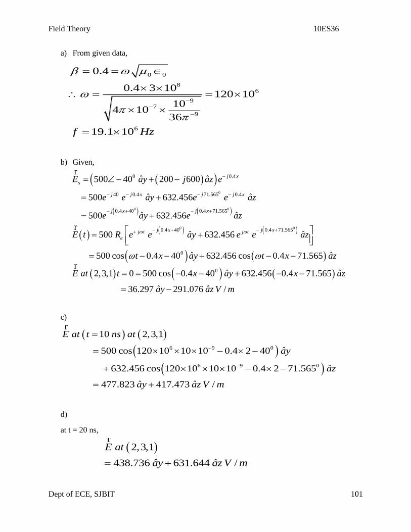
Field Theory 10ES36


a) From given data,

0 0

86

97

9

6

0.4

0.4 3 10120 10

104 10

36

19.1 10f Hz

b) Given,

0

0 0

0 0

0 0.4

40 0.4 71.565 0.4

0.4 40 0.4 71.565

0.4 40 0.4 71.565

ˆ ˆ500 40 200 600

ˆ ˆ500 632.456

ˆ ˆ500 632.456

ˆ ˆ500 632.456

500 cos 0

j x

s

j j x j j x

j x j x

j x j xj t j t

e

E ay j az e

e e ay e e az

e ay e az

E t R e e ay e e az

t

r

r

0

0

ˆ ˆ.4 40 632.456 cos 0.4 71.565

ˆ ˆ2,3,1 0 500 cos 0.4 40 632.456 0.4 71.565

ˆ ˆ36.297 291.076 /

x ay t x az

E at t x ay x az

ay az V m

r

c)

6 9 0

6 9 0

10 2,3,1

ˆ500 cos 120 10 10 10 0.4 2 40

ˆ632.456 cos 120 10 10 10 0.4 2 71.565

ˆ ˆ477.823 417.473 /

E at t ns at

ay

az

ay az V m

r

d)

at t = 20 ns,

2,3,1

ˆ ˆ438.736 631.644 /

E at

ay az V m

r

Field Theory 10ES36


Example:

Given 0 0.07ˆ ˆ2 40 3 20 /j z

sH ax ay e A m r

for a UPW traveling in free space. Find

(a) (b) Hx at p(1,2,3) at t = 31 ns. (c) Hr

at t=0 at the origin.

(a) we have p = 0.07 ( )j ze term

8 6

6

0.07

0.070.07 3 10 21.0 10 / sec

21.0 10 / sec

rad

rad

(b)

0 040 0.07 20 0.07

0 0

0

6 0

6 9 0

3

ˆ ˆ2 3

ˆ ˆ2 cos 0.07 40 3 cos 0.07 20

( ) 2cos 0.07 40

( ) 1,2,3

2cos 2.1 10 0.21 40

31 sec; 2cos 2.1 10 31 10 0.21 40

2cos 651 10

j j z j j z j t

e

x

x

H t R e e ax e e ay e

t z ax t z ay

H t t z

H t at p

t

At t n

r

00.21 40

1.9333 /A m

(c)

ˆ ˆ0 2cos 0.07 0.7 3cos 0.7 0.35

ˆ ˆ2cos 0.7 3cos 0.3

ˆ ˆ1.53 2.82

3.20666 /

H t at t z ax z ay

H t ax ay

ax ay

A m

r

r

In free space,

Field Theory 10ES36


ˆ, 120sin /

,

120

120ˆsin

120 120

1sin

1ˆ, sin

y

x

y

x

E z t t z ay V m

find H z t

Ewe have

H

EH t z ay

t z

H z t t z ax

r

Problem 3:

Non uniform plans waves also can exist under special conditions. Show that the function

sinzF e x t

satisfies the wave equation 2

2

2 2

1 FF

c t

provided the wave velocity is given by

2 2

21

ce

Ans:

From the given eqn. for F, we note that F is a function of x and z,

2 22

2 2

2 2

2 2

22 2

2

cos

sin

sin

sin

z

zz

z

z

F FF

x y

Fe x t

x

F ee x t F

x

Fe x t

z

Fe x t F

z

Field Theory 10ES36


22 2

2

2

2

2

cos

sin

z

z

F F

dFe x t

dt

d Fe x t

dt

F

The given wave equation is

22

2 2

22 2

2 2

2 22

2 2

2 22

2 2

22

22

2

2 2 22

2 22 2 2

2

2 2

2

1

1

1

1

FF

c t

F Fc

c

c

c

c c

cc

cor

c

Example

The electric field intensity of a uniform plane wave in air has a magnitude of 754 V/m and is

in the z direction. If the wave has a wave length = 2m and propagating in the y direction.

Find

(i) Frequency and when the field has the form cosA t z .

(ii) Find an expression for Hr

.

Field Theory 10ES36


In air or free space,

83 10 / secc m

(i)

88

6

3 10/ sec 1.5 10 150

2

2 23.14 /

2

754cos 2 150 10z

ef m Hz MHz

m

rad mm

E t y

(iii) For a wave propagating in the +y direction,

xz

z z

EE

H H

For the given wave,

6

754 / ; 0

754 754754 /

120 377

ˆ2cos 2 150 10 /

z x

x

E V m E

H A m

H t y ax A m

r

Example

find for copper having = 5.8*107 (/m) at 50Hz, 3MHz, 30GHz.

7 7

3

2 2

33

35

6

37

6

2 1

1 1 1 1

4 10 5.8 10

1 1 1 66 10

4 5.8 23.2

66 10( ) 9.3459 10

50

66 10( ) 3.8105 10

3 10

66 10( ) 3.8105 10

3 10

f

f

f f f

i m

ii m

iii m

Field Theory 10ES36


Wave Propagation in a loss less medium:

Definition of uniform plane wave in Phasor form:

In phasor form, the uniform plane wave is defined as one for which the equiphase surface is

also an equiamplitude surface, it is a uniform plane wave.

For a uniform plane wave having no variations in x and y directions, the wave equation in

phasor form may be expressed as

2 22 2

2 20 ________ ( )

E EE r E i

Z Z

r rr r

where . Let us consider eqn.(i) for, the Ey component, we get

2

2

2

y

y

EE

Z

yE has a solution of the form,

1 2 ________ (2)j z j z

yE C e C e

Where C1 and C2 are arbitrary complex constants. The corresponding time varying form of

yE is

1 2

,

_______ (3)

j t

y e y

j z j z j t

e

E z t R E z e

R C e C e e

%

If C1 and C2 are real, the result of real part extraction operation is,

1 2, cos cos _______ (4)yE z t C t z C t z

From (3) we note that, in a homogeneous lossless medium, sinusoidal time variation results

in space variations which is also sinusoidal.

Equations (3) and (4) represent sum of two waves traveling in opposite directions.

If C1 = C2, the two wave combine to form a standing wave which does not progress.

Phase velocity and wavelength:

The wave velocity can easily obtained when we rewrite Ey as a function and z t , as in

eqn. (4). This shows that

Field Theory 10ES36


________(5)

In phasor form, identifying a some reference point on the waveform and observing its

velocity may obtain the same result. For a wave traveling in the +Z direction, this point is

given by t z a constant.

dz

dt

, as in eqn. (5)

This velocity of some point on the sinusoidal waveform is called the phase velocity. is

called the phase-shift constant and is a measure of phase shift in radians per unit length.

Wavelength: Wavelength is defined as that distance over which the sinusoidal waveform

passes through a full cycle of 2 radius.

ie.,

2

2 2 2 1; ________(7)

2

, ________(8)

ff

f f in Hz

For the value of given in eqn. (1), the phase velocity is,

0

8

0

1_______(9)

; 3 10 / secC C m

Wave propagation in conducting medium:

The wave eqn. written in the form of Helmholtz eqn. is

2 2

2 2

0 _______(10)

_______(11)

E E

where j j j

r r

.

, the propagation constant is complex = + j _________(12)

We have, for the uniform plane wave traveling in the z direction, the electric field Er

must

satisfy

Field Theory 10ES36


22

2_______(13)

EE

Z

rr

This equation has a possible solution

0 _______(14)ZE Z E e r

In time varying form this is becomes

0, _______(15)Z j t

eE z t R E e e r%

= 0 ________(16)

j t zz

ee R E e

This is the equation of a wave traveling in the +Z direction and attenuated by a factor Ze .

The phase shift factor and the wavelength phase, velocity, as in the lossless case, are given

by

2f

The propagation constant

We have, ________(11)j j

22 2 2 22 ________(17)j j j

2 2 2 2 2 2; ________(18)

________(19)2

Therefore (19) in (18) gives:

Field Theory 10ES36


2

2 2

4 2 2 2 2 2

2 2 24 2 2

2 4 2 2 2 2 2

2

2 22 2

2

2 2 2

2 2

2

2 2

2

2 2

4

4 4 0

04

2

1

2

1 12

1 1 _________(20)2

1 1 _______2

and

____(21)

We choose some reference point on the wave, the cosine function,(say a rest). The value of

the wave ie., the cosine is an integer multiple of 2 at erest.

0 2k z m at mth

erest.

Now let us fix our position on the wave as this mth

erest and observe time variation at this

position, nothing that the entire cosine argument is the same multiple of 2 for all time in

order to keep track of the point.

ie., 0 0 2 /t k z m t z c

Thus at t increases, position z must also increase to satisfy eqn. ( ). Thus the wave erest (and

the entire wave moves in a +ve direction) with a speed given by the above eqn.

Field Theory 10ES36


Similarly, eqn. ( ) having a cosine argument 0t z describes a wave that moves in the

negative direction (as + increases z must decrease to keep the argument constant). These two

waves are called the traveling waves.

Let us further consider only +ve z traveling wave:

We have

ˆˆ ˆ

0 0

0x y

i j k

x y z

E E

0 0

0 0

0

00 0

0

00 0

0

0

ˆ

1

, cos

; 377 120

s s

y xy

xsy

jk z j z

oy z x

y x

x

y

E j H

E Ei j k j iH x j b

z z

Ej H

z

H E e E ej

H z t E t z

E

H

r r

Ey and Hx are in phase in time and space. The UPW is called so because is uniform thought

any plane Z = constant.

Energy flow is in +Z direction.

E and H are perpendicular to the direction of propagation; both lie in a plane that is

transverse to the direction of propagation. Therefore also called a TEM wave.

Example: The electric field amplitude of a UPW in the az direction is 250 V/m. If Er

=

ˆxE ax and = 1m rad/sec, find (i) f (ii) (iii) period (iv) amplitude of H

r.

Field Theory 10ES36


62 10159.155

2 2 2

1.88495

16.283

120

2500.6631 /

120 120

xy

y

xy

ff KHz

Ckm

f

period sf

Eamplitude of H

H

EH A m

11.2. Given 0 0 0.07ˆ ˆ2 40 3 20 /j z

sH ax ay e A m r

for a certain UPW traveling in free

space.

Find (i), (ii)Hx at p(1,2,3) at t = 31ns and (iii) Hr

at t = 0 at the orign.

Wave propagation in dielectrics:

For an isotopic and homogeneous medium, the wave equation becomes

2 2

0 0

s s

r r r r

E k

k k

r

For Ex component

We have

22

2

xsxs

d Ek E

dz for Ex comp. Of electric field wave traveling in Z – direction.

k can be complex one of the solutions of this eqn. is,

0

z j z

xs x

jk j

E E e e

Therefore its time varying part becomes,

Field Theory 10ES36


0 cosz

xs xE E e t z

This is UPW that propagates in the +Z direction with phase constant but losing its amplitude

with increasing zZ e . Thus the general effect of a complex valued k is to yield a traveling

wave that changes its amplitude with distance.

If is +ve = attenuation coefficient if is +ve wave decays

If is -ve = gain coefficient wave grows

In passive media, is +ve is measured in repers per meter

In amplifiers (lasers) is –ve.

Wave propagation in a conducting medium for medium for time-harmonic

fields: (Fields with sinusoidal time variations)

For sinusoidal time variations, the electric field for lossless medium ( = 0) becomes

2 2E E r r

In a conducting medium, the wave eqn. becomes for sinusoidal time variations:

2 2 0E j E r r

Problem:

Using Maxwell’s eqn. (1) show that

. 0D r

in a conductor

if ohm’s law and sinusoidal time variations are assumed. When ohm’s law and sinusoidal time

variations are assumed, the first Maxwell’s curl equation is

H E j E r r r

Taking divergence on both sides, we get,

0

0

0

, &

H E j E

E j

or D j

are

r r rg g

rg

rg

constants and of finite values and 0

Field Theory 10ES36


0D r

g

POLARISATION:

It shows the time varying behavior of the electric field strength vector at some point in space.

Consider of a UPW traveling along Z direction with Er%

and Hr%

vectors lying in the x-y plane.

If 0Ey % and only Ex% is present, the wave is said to be polarized in the x-direction.

If Ex% = 0 and only Ey% is present, the wave is said to be polarized in the y-direction.

Therefore the direction of Er

is the direction of polarization

If both Ex% and Ey% are present and are in phase, then the resultant electric field Er

has a

direction that depends on the relative magnitudes of Ex% and Ey% .

The angle which this resultant direction makes with the x axis is tan-1

Ey

Ex

%

%; and this angle will be

constant with time.

(a) Linear polarization:

In all the above three cases, the direction of the resultant vector is constant with time and the

wave is said to be linearly polarized.

If Ex% and Ey% are not in phase ie., they reach their maxima at different instances of time, then

the direction of the resultant electric vector will vary with time. In this case it can be shown that

the locus of the end point of the resultant Er%

will be an ellipse and the wave is said to be

elliptically polarized.

In the particular case where Ex% and Ey% have equal magnitudes and a 900 phase difference, the

locus of the resultant Er%

is a circle and the wave is circularly polarized.

Linear Polarisation:

Consider the phasor form of the electric field of a UPW traveling in the Z-direction:

0

j zE Z E e r

Its time varying or instanious time form is

0, j z j t

eE Z t R E e e r%

Field Theory 10ES36


The wave is traveling in Z-direction.

Therefore zE

r lies in the x-y plane. In general,

0Er

is a complex vector ie., a vector whose

components are complex numbers.

Therefore we can write 0Er

as,

0 0r iE E jE r r r

Where 0Er

and 0iE

r are real vectors having, in general, different directions.

At some point in space, (say z = 0) the resultant time varying electric field is

0 0

0 0

0,

cos sin

j t

e r i

r i

E t R E j E e

E t E t

r r r%

r r

Therefore Er

not only changes its magnitude but also changes its direction as time varies.

Circular Polarisation:

Here the x and y components of the electric field vector are equal in magnitude.

If Ey leads Ex by 900 and Ex and Ey have the same amplitudes,

Ie., x yE E , we have, 0ˆ ˆE ax j ay E

r%

The corresponding time varying version is,

0

0

0

2 2 2

0

ˆ ˆ0, cos sin

cos

sin

x

y

x y

E t ax t ay t E

E E t

and E E t

E E E

r r%

Which shows that the end point of 0 0,E tr%

traces a circle of radius 0E as time progresses.

Therefore the wave is said to the circularly polarized. Further we see that the sense or direction

of rotation is that of a left handed screw advancing in the Z-direction ( ie., in the direction of

propagation). Then this wave is said to be left circularly polarized.

Similar remarks hold for a right-circularly polarized wave represented by the complex vector,

0ˆ ˆE ax j ay E

r%

Field Theory 10ES36


It is apparent that a reversal of the sense of rotation may be obtained by a 1800 phase shift

applied either to the x component of the electric field.

Elliptical Polarisation:

Here x and y components of the electric field differ in amplitudes x yE E% % .

Assume that Ey leads Ex by 900.

Then,

0ˆ ˆE ax A j ay B

Where A and B are +ve real constants.

Its time varying form is

22

2 2

ˆ ˆ0, cos sin

cos

sin

1

x

y

yx

E t axA t ayB t

E A t

E B t

EE

A B

r%

%

%

%%

Thus the end point of the 0,E tr%

vector traces out an ellipse and the wave is elliptically

polarized; the sense of polarization is left-handed.

Elliptical polarization is a more general form of polarization. The polarization is completely

specified by the orientation and axial ratio of the polarization ellipse and by the sense in which

the end point of the electric field moves around the ellipse.

Field Theory 10ES36



1. Give the general equation of electromagnetic wave.

2. Derive for Characteristic impedance.

3. Derive equation of uniform Plane wave propagating in free space.

4. Derive equation of uniform Plane wave propagating in perfect dielectric.

5. Derive equation of uniform Plane wave propagating in general medium.

6. Define skin effect.

7. Define skin depth & bring out the relationship between skin depth & frequency.

8. State and prove Poynting theorem.

9. Define Poynting vector.

10. Derive for intrinsic impedance in case of general medium.

Field Theory 10ES36


UNIT – 8

PLANE WAVES AT BOUNDARIES AND IN DISPERSIVE MEDIA

Syllabus:

Reflection of uniform plane waves at normal incidence, SWR, Plane wave propagation in

general directions

REFERENCE BOOKS:


edition,2006.


edition, 1999




2002



.

Reflection of uniform plane waves at normal incidence:

Reflection of uniform plane waves occurs due to mismatch between the characteristic parameters

of the 2 medium.

When a uniform plane plane wave is incident on the boundary between regions composed of 2

different materials, it is partially reflected & partially transmitted. Consider an interface between

region1 and region 2 as shown in the fig 8.1.

We assume that, we have only a single vector component of electric field intensity As shown in

figure, we define region 1, as the half space for which z<0 and region 2 is the other half-space

for which z>0.

Initially, we assume that, wave in a region 1 is travelling in +z direction and linearly polarized

along x. Then the time varying electric field in the x-direction is given by,

in phasor form,

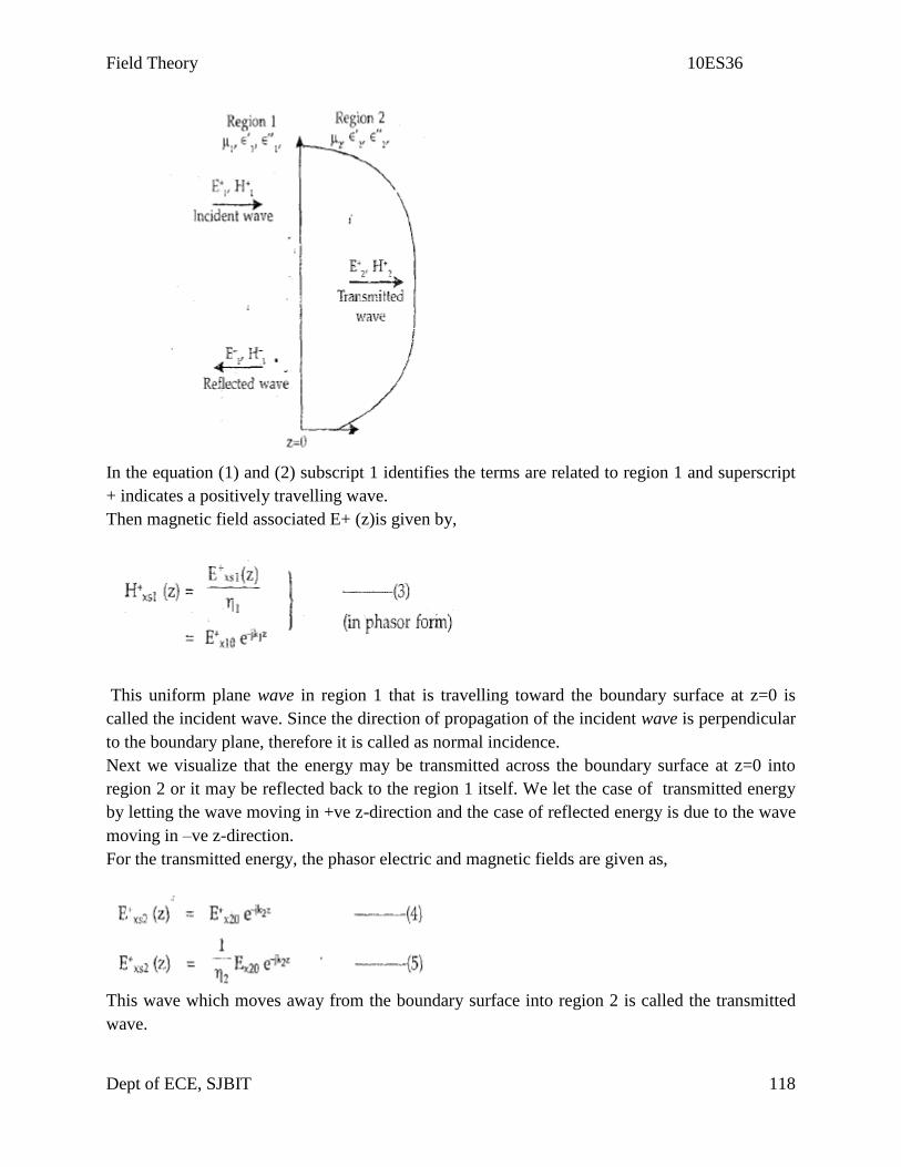
Field Theory 10ES36


In the equation (1) and (2) subscript 1 identifies the terms are related to region 1 and superscript

+ indicates a positively travelling wave.

Then magnetic field associated E+ (z)is given by,

This uniform plane wave in region 1 that is travelling toward the boundary surface at z=0 is

called the incident wave. Since the direction of propagation of the incident wave is perpendicular

to the boundary plane, therefore it is called as normal incidence.

Next we visualize that the energy may be transmitted across the boundary surface at z=0 into

region 2 or it may be reflected back to the region 1 itself. We let the case of transmitted energy

by letting the wave moving in +ve z-direction and the case of reflected energy is due to the wave

moving in –ve z-direction.

For the transmitted energy, the phasor electric and magnetic fields are given as,

This wave which moves away from the boundary surface into region 2 is called the transmitted

wave.

Field Theory 10ES36


Then, a wave travelling away from the boundary in region 1 as shown in figure, in the -ve z-

direction is called as reflected wave as it is directed back to region 1.

Therefore electric & magnetic field quantities of this reflected wave are given as,

Then these quantities to be true, these must satisfy boundary conditions at z=0. In the process,

the tangential electric fields in the region 1 and region 2 must become equal and also H is being

y-directed is also a tangential must be continuous across the boundary. These can be verified

easily by letting z=0 in the above field components.

The total electric field intensity in region 1 and in the region 2 , therefore we have,

Therefore,

For H field , we have

Reflection co-efficient and transmission co-efficient in case of normal incidences:

In this case part of the energy is transmitted and part of the energy is reflected.

Perfect dielectric: = 0. no absorption or loss of power in propagation through the dielectric.

Boundary is parallel to the x = 0 plane.

Plane wave traveling in +x direction is incident on it.

Field Theory 10ES36


We have,

1

1

2

i r

r r

t t

E H

E H

E H

BC: Tang comp. Of E or Hr r

is continuous across the boundary.

ie.,

1 2

2 1

2 1 2 1

2 1

2 1

1

1 2

1 2

1 2

1 1

2 1 2

1 1

2, 1

,

2

i r z

i r t

i r i r z i r

i r i r

i r

r

i

t i r r

i i

r r

t

t t

i i

H H H

E E E

H H E E H E E

E E E E

E E

E

E

E E E EAlso

c E E

H EFurther

H E

H E

H E

The permeabilities of all known insulators do not differ appreciably from that of free space,

so that,

1 2

0 2 0 1 1 2

0 2 0 1 1 2

1

1 2

2 1

2 1

2

1 2

/ /

/ /

2

2

r

i

t

i

r

i

t

i

E

E

E

E

H

H

H

H

Field Theory 10ES36


Standing wave ratio :

It is defined as the ratio of the maximum to minimum amplitudes of electric field components

where standing wave exists. It is denoted by,S. 1f Ex max is the maximum amplitude of electric

field and I Ex, min is the minimum amplitude of electric field then standing wave ratio is given

as,

If y is reflection coefficient, the 'S' is given in terms of y as,

The maximum occurs when each term in the parenthesis in (4) has the same phase angle. So, for

Ex positive and real the maximum is,

The minima occur where the phase angles of the two terms in the parenthesis in (4) differ by

180°, thus the minimum is,

Then by definition of standing wave ratio, it is given as,

Such case of plane wave propagation is one in which incident waves on boundaries are not

normal (or perpendicular) to the propagation direction but propagate in any direction.

Let us consider boundary positioned in the x, y plane and assume that the incident wave will

propagate in a direction that could involve all three co-ordinate axis. With this assumption, let us

consider that the propagating medium is loss-less and propagation phase constant is given by

Field Theory 10ES36


For the simplicity, we consider a two-dimensional case, where the wave travels in a direction

between x and z axes.

Let us consider propagation constant as a vector as K indicated in the figure.

The direction of K is the propagation direction. The magnitude of K is the phase shift per unit

distance along that direction.

In general, the wave propagating in z-direction specified in its phasor form is associated with the

factor

To specify the phase in two-dimensional system, we use vector nature of K. Let us consider the

phase at a general location (x, z) described through a position vector r as shown.in the figure.

Then the phase at location, referenced to the origin is given by the projection of K along r times

the magnitude of r or just k - r. If the electric field is of magnitude Eo, therefore the phasor form

of the wave can be written as,

In two-dimensional case of above figure, k and) can be expressed as,

Therefore,

Therefore equation 1 becomes,

Field Theory 10ES36


The equation (2) is the general form of wave equation specific to the situation, the angle of

propagation from the x-axis is given by,

The figure shows such series of wave fronts with different phase shifts.


1. 1. Derive for reflection co-efficient & transmission co-efficient.

2. Derive for reflection co-efficient & transmission co-efficient for normal incidence at a

plane conducting boundary.

3. Define standing wave ratio.

4. Derive for plane wave propagating in general directions

syllabus - atria | e-learning · field and wave electromagnetics , david k cheng , ... 2nd edition,...

Documents