switching near a network of rotating nodes 1. introduction heteroclinic connections

SWITCHING NEAR A NETWORKOF ROTATING NODES

MANUELA A.D. AGUIAR, ISABEL S. LABOURIAU,AND ALEXANDRE A. P. RODRIGUES

Abstract. We study the dynamics of a Z2⊕Z2- equivariant vec-tor field in the neighbourhood of a heteroclinic network with a peri-odic trajectory and symmetric equilibria. We assume that aroundeach equilibrium the linearization of the vector field has non-realeigenvalues. Trajectories starting near each node of the networkturn around in space either following the periodic trajectory or dueto the complex eigenvalues near the equilibria. Thus, a networkwith rotating nodes. The rotations combine with transverse inter-sections of two-dimensional invariant manifolds to create switchingnear the network: close to the network there are trajectories thatvisit neighbourhoods of the saddles following all the heteroclinicconnections of the network in any given order. Our results are mo-tivated by an example where switching was observed numerically,by forced symmetry breaking of an asymptotically stable networkwith O(2) symmetry.

1. Introduction

Heteroclinic connections and networks are a common feature of sym-metric differential equations, and persist under perturbations that pre-serve the symmetry. Start with an asymptotically stable network withO(2) symmetry. A perturbation that breaks part of the symmetrysplits a two-dimensional connection into a pair of one-dimensional ones.The new network is no longer asymptotically stable, nearby trajectoriesfollow the network around in a complex way that we call switching.

By a heteroclinic network we mean a connected flow-invariant setthat is the union of heteroclinic cycles. In the present case it is theorbit under the symmetry group Z2 ⊕Z2 of a heteroclinic cycle. These

2000 Mathematics Subject Classification. Primary: 37G30; Secondary: 37C10,34C37, 37C29, 34C28, 37C80.

Key words and phrases. heteroclinic network , switching , vector fields , symme-try breaking , shadowing.

The research of all authors at Centro de Matematica da Universidade doPorto (CMUP) had financial support from Fundacao para a Ciencia e a Tec-nologia (FCT), Portugal, through the programs POCTI and POSI with Euro-pean Union and national funding. A.A.P. Rodrigues was supported by the grantSFRH/BD/28936/2006 of FCT.

1

2 M.A.D.AGUIAR, I.S.LABOURIAU, AND A.A.P.RODRIGUES

networks are often called heteroclinic cycles in the literature. Hete-roclinic cycles and networks are known to occur persistently in thesettings of symmetry [8], [16], coupled cell systems (with and withoutsymmetry) [6], [2] and population dynamics [12], [13], [11], [7]. Theyare induced by the existence of flow invariant subpaces that correspond,respectively, to fixed point subspaces, synchrony subspaces and coor-dinate axes and hyperplanes.

We study the dynamics near such a network where all cycles havea common node that is a closed trajectory. We prove that there aretrajectories near the network that follow its cycles in any desired or-der. Trajectories that go near the periodic orbit may switch to anyheteroclinic cycle, return and switch again.

It is worthwhile to isolate general properties that entail switching,so the results may be applied to examples in other contexts.

There exist in the literature several numerical reports on complicateddynamics near heteroclinic networks of equilibria and of equilibria andperiodic trajectories, that include random visits to the nodes of thenetwork in any possible order [10], [8], [5], [23].

This type of behaviour is not possible around asymptotically sta-ble heteroclinic networks whose connections are contained in invariantsubspaces. Each cycle in the network cannot be asymptotically stablebut it may have strong attractivity properties [19], [24] so that eachnearby trajectory outside the invariant subspaces will tend to one ofthe cycles in the network.

Different forms of switching have been described in several contexts.Networks where all the nodes are equilibria, have been studied byPostlethwaite and Dawes [21] who found trajectories that follow threecycles in a network sequentially, both regularly and irregularly; by Kirkand Silber [15] near a network with two cycles who found nearby tra-jectories that switch in one direction. Persistent random switching isfound by Guckenheimer and Worfolk [10] and Aguiar et al [4]; noiseinduced switching in Armbruster et al [5].

A problem similar to ours, where a network involves equilibria and aperiodic trajectory, appears in the heteroclinic model of the geodynamoderived in Melbourne et al [20]. Starting with a model with Z2 ⊕Z2 ⊕ SO(2) symmetry, they perturb the model so the only remainingsymmetry is −Id. For the perturbed model they establish switchingnumerically in terms of reversals and excursions.

This has motivated Kirk and Rucklidge [14] to ask whether switch-ing would be observed when all the symmetries are broken. First theyanalyse partially broken symmetries in two different ways: when onlythe SO(2) symmetry remains they find a weak form of switching, wheretrajectories starting near one equilibrium may visit the neighbourhoodof another but not return to the first one; for the Z2 ⊕ Z2 symmet-ric case they find attracting periodic trajectories and no switching.

SWITCHING NEAR A NETWORK 3

Then they argue that when all symmetries are broken and the net-work is destroyed, switching will not take place arbitrarily close toZ2 ⊕ Z2-symmetric problems because of barriers formed by invariantmanifolds. They describe a scenario where switching may arise, if thesymmetry-breaking terms are larger than a threshold value. They pro-pose a mechanism for switching arising from the right combination ofhomoclinic tangencies between the stable and unstable manifolds of aperiodic orbit and specific heteroclinic tangencies between stable andunstable manifolds of the equilibria.

Here we analyse equations with a symmetry group Z2⊕Z2 a subgroupof that considered by Melbourne et al [20] but not acting in the sameway as in Kirk and Rucklidge [14]: each Z2 in our setting containsa rotation by π that fixes a plane. A discussion of how our resultscompare with those of [14] and [20] appears at the end of this paper insection 9.

Under generic hypotheses for this symmetry, we prove a strong formof switching: the existence of trajectories that visit neighbourhoods ofany sequence of nodes of the network in any order that is compatiblewith the network connections.

The conditions we need for switching are stated in section 3 precededby definitions and preliminary results in section 2.

In section 4 we present an example of a Z2 ⊕Z2- equivariant familyof ordinary differential equations having a network of rotating nodes.When one of the parameters is set to zero, the equations are Z2 ⊕Z2 ⊕SO(2)-symmetric and the network is asymptotically stable. Switchingoccurs for all small non-zero values of this symmetry-breaking param-eter.

We linearize the flow around the invariant saddles in section 5, ob-taining isolating blocks around each node of the network. This sec-tion is mostly concerned with introducing the notation for the proof ofswitching that occupies the rest of the paper.

The goal of this paper is to prove switching in the neighbourhoodof a heteroclinic network that consists of four symmetric copies of aheteroclinic cycle

C → v → w → C

where C is a closed trajectory invariant under the symmetries and vand w are equilibria. The connection v → w is one-dimensional andtakes place inside a fixed-point subspace, the other connections aretransverse intersections of 2-dimensional invariant manifolds. The tra-jectory C has real Floquet multipliers and 2-dimensional stable andunstable manifolds; the linearisation of the flow near v has a pairof complex eigenvalues with positive real part and one real negativeeigenvalue; the linearisation of the flow near w has one real positiveeigenvalue and pair of complex eigenvalues with negative real part (seefigures 1 and 2).


In section 6 we obtain a geometrical description of the way the flowtransforms a curve of initial conditions lying across the stable manifoldof each node. The curve is wrapped around the isolating block of thenext node, accumulating on its unstable manifold and in particular onthe next connection. Thus, points on a line across the stable manifoldof v will be mapped into a helix accumulating on the unstable manifoldof w that will cross the transverse stable manifold of C infinitely manytimes. Similarly, points on a line across the stable manifold of C willbe mapped into a helix accumulating on its unstable manifold and thuswill cross the transverse stable manifold of v infinitely many times.

The geometrical setting is explored in section 7 to obtain intervalson the curve of initial conditions that are mapped by the flow intocurves near the next node in a position similar to the first one. Thisallows us to establish the recurrence needed for switching in section 8:for any sequence of nodes like

+v → −w → C → −v → −w → C → +v → +w → C → +v → · · ·

we find a trajectory that visits neighbourhoods of these nodes in thesame sequence.

We end the paper with a discussion (section 9) of the results obtainedand of related results in the literature.

2. Preliminaries

Let f be a smooth vector field on Rn with flow given by the uniquesolution x(t) = ϕ(t, x0) ∈ Rn of

(1) x = f(x) x(0) = x0.

If A is a compact invariant set for the flow of f , we say, followingField [8], that A is an invariant saddle if

A ⊆ W s(A)\A and A ⊆ W u(A)\A,

where A is the closure of A. In this paper all the saddles are hyperbolic.Given two invariant saddles A and B, an m-dimensional hetero-

clinic connection from A to B, denoted [A → B], is an m-dimensionalconnected flow-invariant manifold contained in W uA)∩W s(B). Theremay be more than one connection from A to B.

Let S ={Aj : j ∈ {1, . . . , k}} be a finite ordered set of mutuallydisjoint invariant saddles. Following Field [8], we say that there is aheteroclinic cycle associated to S if

∀j ∈ {1, . . . , k}, W u(Aj) ∩ W s(Aj+1) 6= ∅ (mod k).

We refer to the saddles defining the heteroclinic cycle as nodes.A heteroclinic network is a finite connected union of heteroclinic

cycles.Let Γ be a compact Lie group acting linearly on Rn. The vector

field f is Γ−equivariant if for all γ ∈ Γ and x ∈ Rn, we have f(γx) =


γf(x). In this case γ ∈ Γ is said to be a symmetry of f . We refer thereader to Golubitsky, Stewart and Schaeffer [9] for more informationon differential equations with symmetry.

The Γ-orbit of x0 ∈ Rn is the set Γ(x0) = {γx0, γ ∈ Γ} that isinvariant under the flow of Γ-equivariant vector fields f . In particular,if x0 is an equilibrium of (1), so are the elements in its Γ-orbit.

The isotropy subgroup of x0 ∈ Rn is Γx0= {γ ∈ Γ, γx0 = x0}. For

an isotropy subgroup Σ of Γ, its fixed-point subspace is

Fix(Σ) = {x ∈ Rn : ∀γ ∈ Σ, γx = x}.

Fixed-point subspaces are the reason for the robustness of heterocliniccycles and networks in symmetric dynamics: if f is Γ-equivariant thenFix(Σ) is flow-invariant, thus connections occurring inside these spacespersist under perturbations that preserve the symmetry.

For a heteroclinic network Σ with node set A, a path of order k, onΣ is a finite sequence sk = (cj)j∈{1,...,k} of connections cj = [Aj → Bj ]in Σ such that Aj , Bj ∈ A and Bj = Aj+1 i.e. cj = [Aj → Aj+1]. Foran infinite path, take j ∈ N.

Let NΣ be a neighbourhood of the network Σ and let UA be a neigh-bourhood of each node A in Σ. For each heteroclinic connection in Σ,consider a point p on it and a small neighbourhood V of p. We areassuming that the neighbourhoods of the nodes are pairwise disjoint,as well for those of points in connections.

Given neighbourhoods as above, the point q, or its trajectory ϕ(t),follows the finite path sk = (cj)j∈{1,...,k} of order k, if there exist twomonotonically increasing sequences of times (ti)i∈{1,...,k+1} and (zi)i∈{1,...,k}

such that for all i ∈ {1, . . . , k}, we have ti < zi < ti+1 and:

(1) ϕ(t) ⊂ NΣ for all t ∈ (t1, tk+1);(2) ϕ(ti) ∈ UAi

and ϕ(zi) ∈ Vi and(3) for all t ∈ (zi, zi+1), ϕ(t) does not visit the neighbourhood of

any other node except that of Ai+1.

There is finite switching near Σ if for each finite path there is atrajectory that follows it. Analogously, we define infinite switchingnear Σ by requiring that each infinite path is followed by a trajectory.

An infinite path on Σ may also be seen as a pseudo-orbit of x = f(x),with infinitely many discontinuities. Switching near Σ means that theseinfinite pseudo-orbits can be shadowed.

3. A network of rotating nodes

Our object of study is the dynamics around a special type of hete-roclinic network (see figure 2) for which we give a rigorous descriptionhere. The network lies in a topological three-sphere and one of its nodesis a closed trajectory with real Floquet multipliers and 2-dimensionalstable and unstable manifolds. Near this node, the flow rotates follow-ing the closed trajectory. The other nodes are equilibria with a pair


+v-v

+w

-w

O

Fix(Z ( ))2 γ 2

(P3) (P4)

Fix(Z ( ))2 γ 1

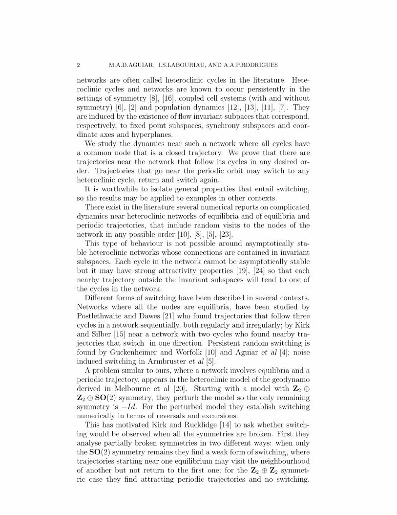
Figure 1. Dynamics near a heteroclinic network ofrotating nodes. Left: dynamics around the planeFix(Z2(γ1)) illustrating property (P3); Right: dynam-ics in the plane Fix(Z2(γ2)) illustrating property (P4).

of non-real eigenvalues. Thus the local dynamics rotates around eachnode.

Specifically, we study a smooth vector field f on R4 with the follow-ing properties:

(P1) The vector field f is equivariant under Γ ∼= Z2 ⊕ Z2 acting lin-early on R4 with generators γ1 and γ2 and with two transverse two-dimensional fixed-point subspaces. In particular, the origin is an equi-librium.

(P2) There is a three-dimensional flow-invariant manifold S3 diffeomor-phic to a sphere that attracts all the trajectories except the origin. Forsimplicity, we assume this manifold to be the unit sphere.

By (P1–P2) there are two flow-invariant circles

C1 = S3 ∩ Fix(Z2(γ1)) and C = S3 ∩ Fix(Z2(γ2)).

(P3) On C1 there are exactly four equilibria that will be denoted by+v, +w, −v = γ2 · v, −w = γ2 · w. Moreover, the eigenvalues of dfrestricted to TS3 are:

• −Cv ± i and Ev with Cv 6= Ev > 0, at ±v;• Ew ± i and −Cw with Cw 6= Ew > 0, at ±w.

In Fix(Z2(γ1)) the equilibria ±v are saddles and ±w are sinks withconnections in C1 from ±v to ±w. These connections are persistentunder perturbations that preserve the γ1−symmetry (see figure 1).


(P4) In the invariant plane Fix(Z2(γ2)) the only equilibrium is theorigin and it is an unstable focus.

Thus C is a closed trajectory and, from (P2), this trajectory is a sinkin Fix(Z2(γ2)) (see figure 1). Since C is contained in the flow-invariantplane Fix(Z2(γ2)), its Floquet multipliers are real.

(P5) The periodic trajectory C is hyperbolic and, in S3, dim W u(C) =dim W s(C) = 2. Moreover, there are connections [C → +v] and[+w → C] satisfying:

W u(C) ⋔ W s (+v) and W u (+w) ⋔ W s (C) .

These intersections are one-dimensional and consist of one pair of γ1-related trajectories.

From the γ2− symmetry, we obtain a pair of γ1-related one-dimensionalconnections in W u(C) ⋔ W s (−v) and in W u (−w) ⋔ W s (C). It fol-lows that there is a heteroclinic network Σ involving the saddles ±v,±w and C (figure 2). Such a network Σ is what we call a network ofrotating nodes. This paper shows switching near this network.

The symmetry γ1 and its flow invariant fixed point subspace ensurethe persistence of the connections [±v → ±w]. The other symmetryγ2 is not essential for the existence of a robust network with theseproperties but it makes them more natural as illustrated by the examplein section 4. The same is true for the existence of the invariant 3-sphere.In section 9 we discuss variants of these hypotheses for which switchingmay be proved in the same way. Note that if the invariant manifoldsW u(C) and W s (−v) did not intersect at all, one of them might forma barrier in S3, contradicting some of the other hypotheses.

4. Example

Our study was initially motivated by the following example con-structed in Aguiar [1], using the methods of [3]. This is an ordinarydifferential equation in R4 given by:

x1 = x1(α1 + α2r21 + α3x

23 + α4x

24 + α5(x

43 − r2

1x24)) − x2

x2 = x2(α1 + α2r21 + α3x

23 + α4x

24 + α5(x

43 − r2

1x24)) + x1

x3 = x3(α1 + α2x23 + α3x

24 + α4r

21 + α5(x

44 − r2

1x23)) + ξh1(x)

x4 = x4(α1 + α2x24 + α3r

21 + α4x

23 + α5(r

41 − x2

3x24)) − ξh2(x)

where x = (x1, x2, x3, x4) ∈ R4, r21 = x2

1 + x22 and

h1(x) = [α1+3α2(x2

1+x2

2)]x1x2x4 and h2(x) = [α1+3α2(x2

1+x2

2)]x1x2x3.

The symmetries of the equation are changes of sign of pairs of coordi-nates:

γ1(x) = (−x1,−x2, x3, x4) γ2(x) = (x1, x2,−x3,−x4).


+ v

+ w

C

- w

- v

Figure 2. Schematic description of a heteroclinic net-work of rotating nodes satisfying (P1)-(P5). Each ar-row represents a 1-dimensional heteroclinic connection.There is one 1-dimensional heteroclinic connection fromeach equilibrium ±v to each equilibrium ±w (P3). Thereare two 1-dimensional heteroclinic connection involvingeach equilibrium and the periodic trajectory C (P5).

In [1] it is proved that, for parameter values such that

α1 > 0 α3 + α4 = 2α2 α3 < α2 < α4 < 0

α2(α3 − α4) + α1α5 > 0

and if ξ ≥ 0 is such that

ξ <−α2α3 + α2α4 + α1α5

2α1α2

and ξ2 <(α4 − α3)(2α1α5 − α2α3 + α2α4)

4α21α2

,

then its dynamics satisfies (P1–P4) as we proceed to explain.For ξ = 0 the equation has more symmetry, like the model in Mel-

bourne et al [20]: it is equivariant under the group Z2 ⊕ Z2 ⊕ SO(2),generated by

κϕ(x) = (x1 cos(ϕ) − x2 sin(ϕ), x1 sin(ϕ) + x2 cos(ϕ), x3, x4)κ2(x) = (x1, x2,−x3, x4) κ3(x) = (x1, x2, x3,−x4).

For ξ = 0 the three-dimensional sphere S3

r of radius r =√

−α1

α2

is flow

invariant and globally attracting. The equilibria ±v (resp. ±w) lieat the intersection of S3

r with line fixed by the subgroup generated byκϕ and κ2 (resp. κϕ and κ3). The closed trajectory C is the intersec-tion of S3

r with the plane fixed by the subgroup generated by κ2 andκ3. A direct computation of the eigenvalues and eigenvectors showsthat the closed trajectory and the equilibria form a network where thetwo-dimensional unstable (resp. stable) manifold of C coincides withthe two-dimensional stable (resp.unstable) manifold of ±v (resp. ±w).


Since all the heteroclinic connections are contained in fixed point sub-spaces, there is no swicthing. Moreover, the network is asymptoticallystable by the criteria of Krupa and Melbourne [17], [18].

For ξ > 0 the SO(2) symmetry is broken and so are the two-dimensional connections. The only symmetries remaining are γ1 = κπ

and γ2 = κ2κ3. The symmetry-breaking term (0, 0, h1(x), h2(x)) is tan-gent to the invariant sphere so it is still flow invariant and properties(P1) and (P2) hold. The perturbation mantain the flow-invariance ofthe lines that were fixed by κ2 and κ3, and the equilibria and the pe-riodic trajectory are preserved together with their stability, and prop-erties (P3-P4) hold. Using Melnikov’s Method, Aguiar [1] proved thatthe two-dimensional manifolds of the periodic trajectory and of thesaddle-foci intersect transversely. Hence property (P5) holds.

5. Local Dynamics near the saddles

Here and in the next two sections, we define the setup for the proofof swicthing near the network. This section contains mostly notationand coordinates used in the rest of the paper.

We restrict our study to S3 since this is a compact and flow-invariantmanifold that captures all the dynamics. When we refer to the sta-ble/unstable manifold of an invariant saddle, we mean the local sta-ble/unstable manifold of that saddle.

We use Samovol’s theorem to linearize the flow around each saddle— equilibrium or closed trajectory. We then introduce local cylindricalcoordinates and define a neighbourhood with boundary transverse tothe linearised flow. For each saddle, we obtain the expression of thelocal map that sends points in the boundary where the flow goes in,into points in the boundary where it goes out. These expressions will beused in the sequel to obtain a geometrical description of the discretisedflow.

5.1. Coordinates near equilibria. Let v and w stand for any of thetwo symmetry-related equilibria ±v and ±w, respectively. By Samo-vol’s theorem [22] f may be linearized around them, since nonresonanceis automatic here. In cylindrical coordinates (ρ, θ, z) the linearizationstake the forms:

(2)

ρ = −Cvρ

θ = 1z = Evz

ρ = Ewρ

θ = 1z = −Cwz.

We consider cylindrical neighbourhoods of v and w in S3 of radiusε > 0 and height 2ε. Their boundaries consist of three components(see figure 3):

• The cylinder wall parametrized by x ∈ R (mod 2π) and |y| ≤ εwith the usual cover (x, y) 7→ (ε, x, y) = (ρ, θ, z).


(a) (b)

2ε

x

y

εr

ϕ

Figure 3. Coordinates on the boundaries of the neigh-bourhood of v and w: (a) cylinder wall (b) top and bot-tom.

• Two disks, the top and the bottom of the cylinder. We takepolar coverings of these disks: (r, ϕ) 7→ (r, ϕ, jε) = (ρ, θ, z)where j ∈ {−, +}, 0 ≤ r ≤ ε and ϕ ∈ R (mod 2π).

change We use x for the angular coordinate on the cylinder wall soas to avoid confusion with the angular coordinate on the disks whendealing with the local maps.

Note that the two flows defined by (2) have symmetry Z2 ⊕ SO(2)given by z 7→ −z and rotation around the z axis. This is an artifact ofthe linearisation and has nothing to do with the original symmetries,but it will be useful in simplifying statements in the next sections.

5.2. Local dynamics near v. The cylinder wall is denoted H inv . Tra-

jectories starting at interior points of H inv go inside the cylinder in

positive time and H inv ∩ W s(v) is parametrized by y = 0. The set

of points in H inv with positive (resp. negative) second coordinate is

denoted H in,+v (resp. H in,−

v ).The top and the bottom of the cylinder are denoted Hout,+

v andHout,−

v , respectively. Trajectories starting at interior points of eitherHout,+

v or Hout,−v go inside the cylinder in negative time (see figure 4).

After linearization W u(v) is the z-axis, intersecting Hout,+v at the

origin of coordinates of Hout,+v . Trajectories starting at H in,j

v , j ∈{+,−} leave the cylindrical neighbourhood at Hout,j

v . The orientationof the z-axis may be chosen to have [v → jw] meeting Hout,j

v .The local map near v, φv : H in,+

v → Hout,+v is given by

(3) φv(x, y) =(

Kvyδv ,− 1

Evln y + x + 1

Evln(ε)

)

= (r, φ) ,


W (v)s

H in,+

H in,-v

v

H out,+v

v

H out,-v

W (v)u loc

loc

W (v)u loc

W (w)u

H out,+

H out,-w

w

H in,+w

w

H in,-w

W (w)s loc

loc

W (w)s loc

Figure 4. Neighbourhoods of the saddle-foci. Left :once the flow enters the cylinder transversely across thewall H in

v \W sloc(v) it leaves it transversely across the cylin-

der top Hout,+v and bottom Hout,−

v . Right : the flow entersthe cylinder transversely across top H in,+

w \W sloc(w) and

bottom H in,−w \W s

loc(w) and leaves it transversely acrossthe wall Hout

w . Inside the two cylinders the vector field islinear.

where

δv =Cv

Ev

> 0, Kv = ε1−δv > 0 and1

Ev

> 0.

The expression for the local map from H in,−v to Hout,−

v is the same.

5.3. Local dynamics near w. After linearization, W s(w) is the z-axis, intersecting the top and bottom of the cylinder at the origin ofthe coordinates. We denote by H in,j

w , j ∈ {−, +}, the component that[jv → w] ∩ H in,j

w 6= ∅. Trajectories starting at interior points of H in,±w

go inside the cylinder in positive time (see figure 4).Trajectories starting at interior points of the cylinder wall Hout

w goinside the cylinder in negative time. The set of points in Hout

w whosesecond coordinate is positive (resp. negative) is denoted Hout,+

w (resp.Hout,−

w ) and Houtw ∩ W u(w) is parametrized by y = 0. The orienta-

tion of the z-axis may be chosen to have trajectories that start atH in,j

w \W s(w), j ∈ {+,−} leaving the cylindrical neighbourhood at


Hout,jw . The local map near w, φw : H in,+

w \W s(w) → Hout,+w is

φw(r, ϕ) =(

1

Ewln(ε) − 1

Ewln r + ϕ, Kwrδw

)

= (x, y) ,

where

δw =Cw

Ew

> 0, Kw = ε1−δw > 0 and1

Ew

> 0.

The same expression holds for the local map from H in,−w \W s(w) to

Hout,−w .

5.4. Local dynamics near the closed trajectory C. Consider alocal cross section S to the flow at p ∈ C. The Poincare first re-turn map defined on S may be linearized around the hyperbolic fixedpoint p using Samovol’s Theorem. Suspending the linear map yields,in cylindrical coordinates, the differential equations:

(4)

ρ = −CC(ρ − 1)

θ = 1z = ECz

that are locally orbitally equivalent to the original flow. In these co-ordinates, C corresponds to the circle ρ = 1 and z = 0, W s(C) is theplane z = 0 and W u(C) is the cylinder ρ = 1.

We work with a hollow three-dimensional cylindrical neighbourhoodof C with boundary H in

C ∪ HoutC , where trajectories starting in H in

C

(resp. HoutC ) go into the neighbourhood in positive (resp. negative)

small time. In what follows we establish some notation for componentsof the boundary (see figure 5).

The components of H inC are the two cylinder walls, H in

C,+ and H inC,−

locally separated by W u(C) and parametrized by the covering map:

(x, y) 7→ (1 ± ε, x, y) = (ρ, θ, z),

where x ∈ R (mod 2π), |y| < ε. We denote by H inC,+ the component

with ρ = 1 + ε.In these coordinates, H in

C ∩ W s(C) is the union of the two circles

y = 0 in the two components. It divides H inC,+ in two parts, H in,+

C,+ and

H in,−C,+ , parametrized, respectively, by positive and negative y, with a

similar convention for H in,+C,− and H in,−

C,− .

The components Hout,+C and Hout,−

C of HoutC are two anuli, locally

separated by W s(C) and parametrized by the covering:

(r, ϕ) 7→ (r, ϕ,±ε) = (ρ, θ, z),

for 1 − ε < r < 1 + ε and ϕ ∈ R (mod 2π) and where Hout,+C is the

component corresponding to the + sign and HoutC ∩W u(C) is the union

of two circles parametrized by r = 1.


W (C)sloc

C

H out,+

C,+ H out,+

C,-

H in,+C,-

H in,+C,+

H out,-

C,- H out,-

C,+

H in,-C,-

H in,-C,+

H = outC H out,+

C H out,-C U

H = out,+C H out,+

C,+ H out,+C,- U

H = out,-C H out,-

C,+ H out,-C,-

U

H = inC H in

C,+ H inC,- U

H = inC,+ H in,+

C,+ H in,-C,+ U

H = inC,- H in,+

C,- H in,-C,- U

W (C) uloc

W (C) uloc

Figure 5. Neighbourhood of the closed trajectory C.The flow enters the hollow cylinder transversely acrosscylinder walls H in

C,± and leaves it transversely across topHout

C,+ and bottom HoutC,−.

Denote by Hout,kC,+ (resp. Hout,k

C,− ), k ∈ {+,−} the set parametrized by

1 < r < 1 + ε (resp. 1 − ε < r < 1) in Hout,kC . In these coordinates the

local map φC : H in,kC,j → Hout,k

C,j , j, k ∈ {+,−}, is given by

φC(x, y) =

(

jKcyδc + 1,

1

Ec

ln(ε) −1

Ec

ln y + x

)

= (r, ϕ),

where

δc =Cc

Ec

> 0 Kc = ε1−δC > 0 and1

Ec

> 0.

6. Geometry near the saddles

The coordinates and notation of section 3 may now be used to anal-yse the geometry of the local dynamics near each saddle. The manifoldW s(v) separates the cylindrical neighbourhood of v into an upper anda lower component, mapped into neighbourhoods of Pw and −w, re-spectively. We show here that initial conditions lying on a segment onthe upper part of the cylindrical wall around v and ending at W s(v)


are mapped into points on a spiral on the top of the cylinder Houtv

where the flow goes out (figure 6).Initial conditions on a spiral on the top of cylindrical neighbourhood

of w are then shown to be mapped into points on a helix around thecylinder accumulating on W u(w) (figure 6). Since W s(C) is transverseto W u(w), then the helix on Hout,+

w is mapped across W s(C) on H inC

infinitely many times. This will be used in section 7 to obtain, inany segment on H in,+

v , infinitely many intervals that are mapped intosegments on H in

C ending at W s(C).Then the image of a segment ending at W s(C) on one of the walls

of H inC is shown to be mapped into a curve accumulating on W u(C) ∩

HoutC (see figure 7). This curve meets W s(v) infinitely many times by

transversality and it is thus mapped across W s(v) on H inv infinitely

many times. Again, we will use this in section 7 to obtain an infin-itely many intervals that are mapped into segments on H in

v ending atW s(v).

This structure of segments containing intervals that are successivelymapped into segments will allow us to establish a recurrence in section 8and to construct nested sequences of intervals containing the initialconditions for switching.

Definition 1. A segment β on H inv (resp.: H in

C ) is a smooth regularparametrized curve β : [0, 1] → H in

p (resp.: β : [0, 1] → H inC ) , that

meets W s(v) (or W s(C)) transverselly at the point β(1) only and suchthat, writing β(s) = (x(s), y(s)), both x and y are monotonic functionsof s.

The coordinates (x, y) may be chosen so as to make the angularcoordinate x an increasing or decreasing function of s as convenient.

Definition 2. Let U be an open set in a plane in Rn and p ∈ U . Aspiral on U around p is a curve α : [0, 1) → U satisfying lim

s→1−α(s) =

p and such that, if α(s) = (α1(s), α2(s)) are its expressions in polarcoordinates (ρ, θ) around p, then α1 and α2 are monotonic, with

lims→1−

|α2(s)| = +∞.

It follows that α1 is a decreasing function of s.

Proposition 1. A segment β on H in,+v (resp. H in,−

v ) is mapped by φv

into a spiral on Hout,+v (resp. Hout,−

v ) around W u(v).

Proof. Write β(s) = (x(s), y(s)) on H in,+v with y(s) ≥ 0 monotonically

decreasing and choose a parametrization of H in,+v such that x(s) is

monotonically increasing. Then, writing φv(β(s)) = (r(s), θ(s)), it fol-lows from the expression of φv in section 5.2 that r(s) is monotonicallydecreasing while θ(s) is monotonically increasing. From lims→1− y(s) =0 and lims→1− x(s) = x(1) the required limits lims→1− r(s) = 0 andlims→1− θ(s) = +∞ follow. �


W (v)s

W (v)u

H in,+

H in,-v

H out,-v

v

[C v]

W (v)u

H out,+v

v

[C v]

W (w)u

W (w)s

H in,+

H in,-w

H out,-w

w

[w C]

W (w)s

H out,+w

w

[w C]

Figure 6. Local Dynamics near the saddle-foci. Left :Near v, any segment on the cylinder wall is mapped intoa spiral on the top or bottom of the cylinder. Right : Aspiral on the top or bottom of the cylinder near w ismapped into a helix on the cylinder wall accumulatingon W u(w). The double arrows on the segment, spiraland helix indicate correspondence of orientation and notthe flow.

Definition 3. Let a, b ∈ R such that a < b and let H be a surfaceparametrized by a cover (θ, h) ∈ R× [a, b] where θ is periodic. A helixon H accumulating on the circle h = h0 is a curve γ : [0, 1) → H suchthat its coordinates (θ(s), h(s)) are monotonic functions of s with

lims→1−

h(s) = h0 and lims→1−

|θ(s)| = +∞.

Proposition 2. A spiral on H in,+w (resp. H in,−

w ) around W s(w) ismapped by φw into a helix on Hout,+

w (resp. Hout,−w ) accumulating on

the circle Houtw ∩ W u(w).

Proof. Parametrize H in,+w so that a spiral σ(s) = (r(s), θ(s)) around

W s(w) has θ(s) increasing with s. The expression of φw of section 5.3ensures that in φw(σ(s)) = (x(s), y(s)) we have y decreasing with s andx increasing with s. The limits in the definiton of helix follow from theform of φw and from lims→1− r(s) = 0 and lims→1− θ(s) = +∞. �

Proposition 3. A segment β on H in,+C,+ is mapped by φC into a helix

on Hout,+C,+ accumulating on the circle W u(C) ∩ Hout,+

C .

The proof, as in Propositions 1 and 2, consists of using the expressionof φC of section 5.4 after a suitable choice of orientation in H in,+

C,+ . Usingthe symmetries of the linearised flow, it follows that Proposition 3 also


H in,+C,+

W (C) u

W (C)sloc

C

H in,-C,+

Figure 7. Local dynamics near the closed trajectory C.A segment on the wall ending at W s(C) is mapped intoa curve accumulating on W u(C) ∩ Hout

C .

holds for a segment β on H in,+C− and for Hout,+

C− , as well as for a segment β

on H in,−C+

and for Hout,−C+

and for β on H in,−C− and for Hout,−

C− , considering

the circle W u(C) ∩ Hout,−C (see figure 7).

7. First return to v

Let p and q be two nodes of Σ such that there is a connection [p → q].The transition map Ψp,q from Hout

p to H inq follows the trajectory [p → q]

in flow-box fashion. In this section we use this information to puttogether the local behaviour of trajectories that start near ±v. Tosimplify the reading, we omit the − and + signs.

Let P ∈ Houtw be one of the points where [w → C] meets Hout

w . Forsmall a, b > 0, the rectangle

[

−a2, a

2

]

×[

− b2, b

2

]

is mapped diffeomor-phically into Hout

w by the parametrization that maps the origin to P(figure 8). Its image, that we denote by Rw, will be called a rectanglein Hout

w centered at P with height b.The vertical sides of Rw are the images of the segments (±a

2, y) with

y ∈[

− b2, b

2

]

. Rectangles in HoutC centered at a given point are defined

in the same way; we denote them by RC .By Propositions 1 and 2, the map

η = φw ◦ Ψv,w ◦ φv : H inv → Hout

w

maps a segment β on H inv infinitely many times across any small rec-

tangle in Houtw centered at a point in W u(w).


H out,+

v

Ψ v,w

segment

H in,+

w

Rw

W (v)s

w

v W (w)u

[v ]

[w C ]

[C v ]

w

P

Figure 8. Transition from v to w: a segment on H inv is

mapped into spirals on Houtv around W u(v) ∩ Hout

v andW s(w) ∩ H in

w . The spiral is then mapped into a helixon Hout

w accumulating on W u(w) and crossing infinitelymany times a rectangle Rw centered at one of the con-nections starting at w (see also figure 9). Double arrowsindicate orientation of the segment and not the flow.

An admissible family of intervals I = {[ai, bi]}i∈N is one that satisfies

0 < ai < bi < ai+1 < 1 and limi→∞

ai = 1.

Proposition 4. Let Rw be a rectangle in Houtw centered at one point

P of Houtw ∩ [w → C]. For any segment β : [0, 1] −→ H in

v there is anadmissible family of intervals {[σi, ρi]}i∈N such that:

(1) each closed interval [σi, ρi] satisfies η ◦ β([σi, ρi]) ⊂ Rw;(2) each open interval (ρi+1, σi) satisfies η ◦ β((ρi+1, σi)) ∩Rw = ∅;(3) the family of curves {η ◦ β([σi, ρi])} accumulates uniformly on

W u(w) ∩ Rw as i → +∞.

This also holds for the local map around C, with C, φC and C wherewe have written w, η and v.

Proof. Writing (x(s), y(s)) for the coordinates of the helix η ◦ β(s) onthe cylinder wall, we have that y decreases with s and that x(s) can betaken as an increasing function of s by choosing compatible orientationsin H in

v and Houtw and, if necessary, by restricting the domain of β to

a smaller interval (s1, 1). In particular the helix η ◦ β may be seen as


a graph (x, y(x)) where x ∈ [x(0), +∞) and where y is a decreasingfunction of x with limx→∞ y(x) = 0 (figure 9).

x

y

b

Rw RwRw Rw Rw RwRw

2

η(β(σ ))0η(β(ρ ))0 Rw

Figure 9. A helix on a periodic cover of the cylinderwall Hout

w . After it meets the first (shaded) copy of therectangle, the helix will intersect the rectangle at inter-vals whose image accumulates on the curve W u(w), rep-resented here by the x-axis.

On Houtw the rectangle Rw is [n − a/2, n + a/2] × [−b/2, b/2] with

n ∈ N. Let σ0 be the smallest value of s ∈ (s1, 1) such that (x(s), y(s))lies on the left vertical side of Rw, with y(σ0) < b

2as in figure 9. Then

y(s) < b2

for all s ∈ [σ0, 1).The sequences defining the family of intervals are obtained from

points where the helix meets successive copies of the vertical sides ofRw with x(σi) = n0 + i − a/2 and x(ρi) = n0 + i + a/2. The proof forφC is similar. �

Proposition 5. Given a segment β : [0, 1] −→ H inv , a rectangle Rw

of sufficiently small height and the family of intervals {[σi, ρi]}i∈N ofProposition 4. Then for sufficiently large i there are τi with σi < τi < ρi

such that Ψw,C ◦ η(β(τi)) ∈ W s(C) and Ψw,C ◦ η ◦ β maps each one of

the intervals [σi, τi] and [τi, ρi] into a segment on one of the sets H in,+C

and H in,−C . This also holds for ΨC,v ◦ φC : H in

C −→ H in,±v with the

appropriate changes.

Proof. Since W s(C) ∩ Houtw meets W u(w) ∩ Hout

w transverselly (prop-erty (P5)) then if the height of Rw is small, W s(C) does not meet itsvertical sides. Each one of the images η◦β([σi, ρi]) meets W s(C)∩Hout

w


transversely at a single point η◦β(τi), since they accumulate uniformlyon W u(w) ∩ Rw as i → +∞. The monotonicity of the coordinates ofη ◦ β will be preserved by Ψw,C close to W u(w). Each componentof η ◦ β([σi, ρi])\ {η ◦ β(τi)} will be mapped into a segment, one into

each connected component of H in,jC \W s(C). The proof for ΨC,v ◦φC is

analogous. �

8. Switching near the Heteroclinic Network

In this section, we put together the information about the first returnmap to H in

v . In sections 6 and 7 we have found that a segment endingat a stable manifold contains intervals that are mapped into segmentsending at the stable manifold of the next node. Starting with a segmenton in H in

v , here this is used recursively to obtain sequences of nestedintervals containing initial conditions that follow sequences heteroclinicconnections.

We say that the path sk = (cj)j∈{1,...,k} of order k on the network Σ isinside the path tk+l = (dj)j∈{1,...,k+l} of order k + l (denoted sk ≺ tk+l)if cj = dj for all j ∈ {1, . . . , k}.

The family of closed intervals I = {Ii}i∈N is inside the family I ={Ii}i∈N (I < I) if, for all i ∈ N, Ii ⊂ Ii. If I is admissible in the sense

of section 7 and I < I then I is also admissible, provided none of itsintervals consists of a point.

Theorem 6. There is finite switching near the network Σ defined bya vector field satisfying (P1)–(P5).

Proof. Given a path, we want to find trajectories that follow it intothe neighbourhoods of section 5 going through small disks in Hout

v

around W u(±v) and through rectangles in Houtw and Hout

C centeredat the connections. Without loss of generality we only consider pathssk = (cj)j∈{1,...,k} starting with c1 = [±v → ±w].

Take a segment β on H in,±v of points that follow the first connection

c1. We will construct admissible families of intervals I(c1, . . . , cn) ={Ii}i∈N recursively, such that points in β(Ii) follow (c1, . . . , cn) andthe image of β(Ii) by the transition maps is a segment. We will showthat sk ≺ sk+l implies I(sk) > I(sk+l) and thus the process will berecursive.

By Propositions 4 and 5, there is an admissible family of intervalsI(c1, c2) = {Ii}i∈N such that β(Ii) is mapped by Ψw,C ◦ φw ◦ Ψv,w ◦

φv into a segment on H in,±C with the choice of sign appropriate for

the next connection c3. Applying the second part of Propositions 4and 5 to this segment, we obtain an admissible family of intervalsI(c1, c2, c3) < I(c1, c2) corresponding to points that follow (c1, c2, c3)and to intervals that are mapped into a segment on H in,±

v with thechoice of sign appropriate for following the connection c4.


}}}} W (v)

Rw

Rw

Rw

w

W (C)s

W (C)s

W (C)s

W (C)s

β

loc

Rw

Rw

Rw

β

W (C)s

RC {

RC {W (v) loc

s s

segment

Figure 10. On a segment β on H inv , there are infinitely

many small segments that are mapped by η into Rw, eachone containing a point mapped into W s(C). The smallsegments contain smaller ones that are mapped into RC

and this may be continued, forming a nested sequence.

In Proposition 5 we assume the height of the rectangle Rw is smalland we reduce it if necessary. This is done to ensure that inside Rw thestable manifold W s(C) is the graph of a function and thus a helix onlymeets it once at each turn. However, as soon as the choice of height ismade it may be kept throughout the proof and thus the constructionof I(sk) is recursive, proving finite switching near Σ. �

Theorem 7. There is infinite switching near the network Σ defined bya vector field satisfying (P1)–(P5).

Proof. Fix an infinite path s∞ = (cj)j∈N on Σ. For each k ∈ N definethe finite path sk of order k by sk = (cj)j∈ {1,...,k}, with sk ≺ sk+1.From the proof of Theorem 6, for each k we have an admissible familyof intervals I(sk) = {Jki}i∈N such that I(sk) > I(sk+1) and all thepoints in β(Jki) follow sk.

Since we have I(sk) > I(sk+1) then Λ =⋂∞

k=1I(sk) is non-empty

because each set Λi =⋂∞

k=1Jki is non empty. From the definition of

admissible family of intervals, if we take ai ∈ Λi then limi→∞ ai = 1.From the construction we have that β(ai) follows s∞. Thus, we haveobtained a sequence of points β(ai) that accumulate on Σ as i → ∞and that follow the infinite path. �

9. Final remarks and discussion

9.1. Generalisation. Not all assumptions of Section 3 are essentialto prove switching, although some of them simplify the calculations.For instance, the eigenvalues at ±v and ±w may have any imaginary


part, not necessarily 1 as in (P3). The proof also works if at one of thepairs of nodes ±v or ±w the eigenvalues of df are real, as long as theeigenvalues at the other pair of nodes are not real — it is enough to haveone pair of rotating equilibria. Any finite number of one-dimensionalconnections [w → C] and [C → v] could have been used instead of twofor each equilibrium.

The existence of swicthing near a networks may be easily generalisedto a heteroclinic network involving rotating nodes such that each het-eroclinic connection involving a periodic trajectory is transverse andthere are no consecutive non transverse heteroclinic connections on thenetwork.

It is not essential to have (Z2 ⊕ Z2)-equivariance. The symmetry γ2

is used here to obtain the closed trajectory C and the role of γ1 is toguarantee that the one-dimensional connections [v → w] are robust.Symmetries make the existence of the network natural and ensure per-sistence. Switching will hold for any network having the nodes andconnections prescribed here, as long as the remaining assumptions aresatisfied.

Estimates for the transition maps may be refined as in Aguiar et

al. [4] to show that near this network there is a suspended horseshoewith transition map described as a full shift over a countable set ofsymbols. The suspended horseshoe has the same shape as the network.Thus, when the O(2)-symmetry of the example in section 4 is brokenwe have instant chaos. In particular it can be shown that there areperiodic orbits that follow any finite path in the network, but this usestechniques beyond the scope of this paper.

Finite switching is present even when all the local maps are expand-ing, as in the case Cv < Ev, Cw < Ew, CC < EC . This is due to therotation around the nodes and is markedly different from the situationwhere all eigenvalues are real. In the example of section 4 this cor-responds to parameter values where the O(2)-symmetric network is arepeller.

A path on the network can also be shadowed by trajectories inW u(C) (see figure 10) because the local unstable manifold of C meetsH in

v at a segment by the transversality assumption (P5). It also fol-lows that there are infinitely many homoclinic connections involvingthe periodic trajectory C, although there are no homoclinic trajecto-ries involving the equilibria. The geometry of W u(C) gets extremelycomplicated as we move away from C, since it will accumulate on thewhole network, having v, w and C as limit points. A complete descrip-tion of the nonwandering set for this type of flows is in preparation.

9.2. Discussion. Generic breaking of the γ1-symmetry destroys thenetwork, as in [14] and [20], by breaking the connections [v → w]. If theremaining assumptions are still satisfied, a weaker form of switching will


hold: for small symmetry-breaking terms, it may still be possible to findtrajectories that visit neighbourhoods of finite sequences of nodes. Thisis because the spirals on top of the cylinder around w of figure 6 willbe off-centered and will turn a finite number of times around W s(w).From this we may obtain points whose trajectories follow short finitepaths on the network. As W u(v) gets closer to W s(w) (as the systemmoves closer to symmetry) the paths that can be shadowed get longer.

This is in contrast to the findings of Kirk and Rucklidge [14], whoclaim that there can be no switching in generic systems close to thesymmetric case, so a comparison of the settings and results of the twopapers is in order at this point. The first caveat is that the Z2 ⊕Z2 representations are different: in our case Fix(Z2 ⊕ Z2) = {0},and there are two transverse 2-dimensional fixed-point subspaces forthe isotropy subgroups, whereas in [14], Fix(Z2 ⊕ Z2) is a plane withtwo 1-dimensional fixed-point subspaces for the isotropy subgroups. Intheir setting, our symmetries correspond to the group generated by arotation of π in SO(2) and by the product of their Z2 ⊕Z2 generators.Both representations occur in the larger group Z2⊕Z2⊕SO(2) used in[20]. Moreover, we are assuming the existence of an invariant 3-sphere(a natural assumption in the symmetric context, see [8] ) and it is notevident that in their context such a sphere will exist.

However, the difference in the results of [14] and ours indicates thatvector fields with Z2 ⊕Z2 ⊕SO(2) symmetry have codimension higherthan 3 in the universe of general vector fields. This will mean that ingeneral systems close to symmetry what will be observed may dependon the way symmetries are broken and that a lot more needs to bedone before switching is well understood.

References

[1] M. Aguiar, Vector Fields with heteroclinic networks, PhD Thesis, Departa-mento de Matematica Aplicada, Faculdade de Ciencias da Universidade doPorto, 2003

[2] M. Aguiar, P. Ashwin, A. Dias and M. Field, Robust heteroclinic cycles in

coupled cell systems: Identical cells with asymmetric inputs, CMUP preprint2008-06

[3] M. Aguiar, S. B. Castro and I. S. Labouriau, Simple Vector Fields with Complex

Behaviour, Int. Jour. of Bifurcation and Chaos, Vol. 16, Nr.2, 2006[4] M. Aguiar, S. B. Castro and I. S. Labouriau, Dynamics near a heteroclinic

network, Nonlinearity 18, 2005[5] D. Armbruster, E. Stone and V. Kirk, Noisy heteroclinic networks, Chaos, Vol.

13, Nr.1, March 2003[6] P. Ashwin and M. Field, Heteroclinic Networks in Coupled Cell Systems Arch.

Rational Mech. Anal., Vol. 148, 1999, pages 107–143[7] W. Brannath, Heteroclinic networks on the tetrahedron, Nonlinearity, Vol. 7,

1994, pages 1367–1384[8] M. Field, Lectures on bifurcations, dynamics and symmetry, Pitman Research

Notes in Mathematics Series, vol. 356, Longman, 1996


[9] M. I. Golubitsky, I. Stewart, and D. G. Schaeffer, Singularities and Groups in

Bifurcation Theory , Vol. II, Springer, 2000[10] J. Guckenheimer and P. Worfolk, Instant Chaos, Nonlinearity, Vol. 5, 1992,

pages 1211–1222[11] J. Hofbauer, Heteroclinic Cycles in Ecological Differential Equations, Tatra

Mountains Math. Publ., Vol. 4, 1994, pages 105–116,[12] J. Hofbauer, Heteroclinic Cycles on the simplex, Proc. Int. Conf. Nonlinear

Oscillations, Janos Bolyai Math. Soc. Budapest, 1987[13] J. Hofbauer and K. Sigmund, The Theory of Evolution and Dynamical Systems,

Cambridge University Press, Cambridge, 1988[14] V. Kirk and A. M. Rucklidge The effect of symmetry breaking on the dynamics

near a structurally stable heteroclinic cycle between equilibria and a periodic

orbit, Dynamical Systems: An International Journal, 23, 2008, pages 42–74[15] V. Kirk and M. Silber, A competition between heteroclinic cycles, Nonlinearity,

Vol. 7, 1994, pages 1605–1621[16] M. Krupa, Robust Heteroclinic Cycles, J. Nonlinear Sci., 7, 1997, pages 129–

176[17] M. Krupa, and I. Melbourne, Asymptotic Stability of Heteroclinic Cycles in

Systems with Symmetry, Ergodic Theory and Dynam. Sys., Vol. 15, 1995,pages 121–147

[18] M. Krupa and I. Melbourne, Asymptotic Stability of Heteroclinic Cycles in

Systems with Symmetry, II, Proc. Roy. Soc. Edinburgh, 134A, 2004, pages1177–1197

[19] I. Melbourne, An example of a non-asymptotically stable attractor Nonlinear-ity, Vol. 4, 1991, pages 835–844

[20] I. Melbourne, M. R. E. Proctor and A. M. Rucklidge, A heteroclinic model of

geodynamo reversals and excursions Dynamo and Dynamics, a MathematicalChallenge (eds. P. Chossat, D. Armbruster and I. Oprea, Kluwer: Dordrecht,2001, pages 363–370

[21] C. M. Postlethwaite and J. H. P. Dawes, Regular and irregular cycling near a

heteroclinic network Nonlinearity, Vol. 18, 2005, pages 1477–1509[22] V. S. Samovol, Linearization of a system of differential equations in the neigh-

bourhood of a singular point, Sov. Math. Dokl, Vol. 13, 1972, pages 1255–1959[23] Y. Sato, E. Akiyama and J. P. Crutchfield, Stability and diversity in collective

adaptation, Physica D, Vol. 210, 2005, pages 21–57[24] T. Ura, On the flow outside a closed invariant set: stability, relative stability

and saddle sets, Contributions to Differential Equations, vol. III, No. 3, 1964,pages 249-94

(M.A.D.Aguiar) Centro de Matematica da Universidade do Porto, and

Faculdade de Economia da Universidade do Porto, Rua Dr. Roberto

Frias, 4200-464 Porto, Portugal

E-mail address : [email protected]

(I.S. Labouriau and A.A.P. Rodrigues) Centro de Matematica da Univer-

sidade do Porto, and Faculdade de Ciencias da Universidade do Porto,

Rua do Campo Alegre 687, 4169–007 Porto, Portugal

E-mail address, I.S.Labouriau: [email protected] address, A.A.P.Rodrigues: [email protected]

switching near a network of rotating nodes 1. introduction heteroclinic connections

Documents