swinging for the fences: executive reactions to quasi-random
TRANSCRIPT
Swinging for the Fences: Executive Reactions to Quasi-Random Option Grants
February 5, 2013
Abstract
The financial crisis renewed interest in the relation between compensation incentives
and risk taking. We examine whether paying top executives with options induces them
to take more risk. To identify the causal effect of options, we exploit two distinct sources
of variation in option compensation that arise from institutional features of multi-year
grant cycles. We find that a 10 percent increase in the value of new options granted
leads to a 6 percent increase in firm equity volatility. This increase in risk is primarily
driven by an increase in leverage. We also find that an increase in stock options leads
to lower dividend growth with mixed effects on investment and firm profitability.
JEL Classification: M52, J33, G32, G34 Keywords: Executive compensation, Incentives, Risk taking, Corporate governance

Swinging for the Fences: Executive Reactions to Quasi-Random Option Grants⇤
Kelly Shue
† and Richard Townsend
‡
February 5, 2013
Abstract
The financial crisis renewed interest in the relation between compensation incentives
and risk taking. We examine whether paying top executives with options induces them
to take more risk. To identify the causal effect of options, we exploit two distinct sources
of variation in option compensation that arise from institutional features of multi-year
grant cycles. We find that a 10 percent increase in the value of new options granted
leads to a 6 percent increase in firm equity volatility. This increase in risk is primarily
driven by an increase in leverage. We also find that an increase in stock options leads
to lower dividend growth with mixed effects on investment and firm profitability.
JEL Classification: M52, J33, G32, G34 Keywords: Executive compensation, Incentives, Risk taking, Corporate governance
⇤We thank David Yermack for his generosity in sharing data. We are grateful to Marianne Bertrand, Ing-Haw Cheng, Ken French, Ed Glaeser, Steve Kaplan, Toby Moskowitz, Canice Prendergast, Amit Seru, seminar participants at University of Chicago (Booth), Simon and Fraser University, University of California San Diego (Rady) and the Booth Junior Finance Symposium for helpful comments. We thank Matt Turner at Pearl Meyer and Don Delves at the Delves Group for helping us understand the intricacies of executive stock option plans. Menaka Hampole provided excellent research assistance. We acknowledge financial support from the Initiative on Global Markets.
†University of Chicago, Booth School of Business. Email: [email protected]. ‡Dartmouth College, Tuck School of Business. Email: [email protected].

1 Introduction
Stock options had potentially unlimited upside, while the downside was simply
to receive nothing if the stock didn’t rise to the predetermined price. The same
applied to plans that tied pay to return on equity: they meant that executives
could win more than they could lose. These pay structures had the unintended
consequence of creating incentives to increase both risk and leverage.
–Financial Crisis Inquiry Commission
The use of stock options in executive compensation packages surged in the last 30 years.
During the 1990s, stock options became the largest component of executive pay, and by the
year 2000, options accounted for 49% of total compensation for CEOs of S&P 500 compa
nies (Frydman and Jenter, 2010). Today, options continue to be prevalent, accounting for
25 percent of total compensation for these CEOs. Moreover, performance vesting shares,
which have option-like payoff structures, have grown increasingly popular in the 2000s, rep
resenting over 30 percent of equity-linked pay (Bettis, Bizjak, Coles, and Kalpathy, 2012).
Options can affect risk taking in at least two ways. Because options have convex payoffs,
the expected compensation from options increases with volatility. After the recent financial
crisis, many pointed to this effect to argue that options induced firms to take excessive risk.
However, replacing a fixed component of compensation with options also increases an exec
utive’s exposure to the firm’s volatility. This exposure effect pushes risk-averse executives
to reduce their firm’s volatility. We seek to measure the net effect of these two competing
forces. The endogeneity of option pay complicates the task, making it difficult to determine
the direction of any causal relation. We exploit quasi-exogenous variation in option compen
sation that results from institutional features of multi-year compensation cycles to resolve
the endogeneity problem.
1

The common intuition that stock options cause executives to take more risk stems from
the fact that the Black-Scholes value of an option increases in the volatility of the underlying
stock (see, e.g., Haugen and Senbet, 1981; Smith Jr. and Watts, 1982; Smith and Stulz,
1985). However, for an undiversified and risk-averse executive, it is not necessarily utility
maximizing to increase risk in response to option pay. For example, Ross (2004) shows
that, because they can make an executive’s wealth more sensitive to the underlying stock
price, options (and convex fee schedules more generally) have an ambiguous effect on risk
taking incentives. If the executive is risk-averse, this can then lead to what Ross refers to as
a “magnification effect, ” which can outweigh the conventional “convexity effect.” This has
also been noted by Lambert, Larcker, and Verrecchia (1991), Carpenter (2000), and Lewellen
(2006). Thus, it is theoretically unclear whether options should increase or decrease risk
taking in practice.
There is a large empirical literature that explores the relationship between executive
stock options and various measures of risk taking behavior. The evidence remains mixed.
For example, Agrawal and Mandelker (1987) find that firms with higher stock and option
ownership make more variance-increasing acquisitions. DeFusco, Johnson, and Zorn (1990)
find that firms that approve stock option plans exhibit an increase in volatility.1 Subsequent
research has focused on the relation between a manager’s “vega” (the sensitivity of the total
Black-Scholes value of all unexercised options to volatility) and risk taking. Several papers
find a small positive cross-sectional association between vega and leverage (Cohen, Hall, and
Viceira, 2000) as well as stock return volatility (Guay, 1999; Cohen, Hall, and Viceira, 2000).
As Guay (1999) notes, however, vega does not take risk aversion into account. To address
this, Lewellen (2006) assumes that managers have a power utility function and measures the
1Fo r m o r e wo r k a l o n g t h e s e l i n e s , s e e S a u n d e r s , S t r o ck , a n d Tr av l o s ( 1 9 9 0 ) ; M e h r a n ( 1 9 9 2 ) ; M ay ( 1 9 9 5 ) ; Tu f a n o ( 1 9 9 6 ) ; B e r g e r , O f e k , a n d Ye r m a ck ( 1 9 9 7 ) ; D e n i s , D e n i s , a n d S a r i n ( 1 9 9 7 ) ; E s ty ( 1 9 9 7 ) ; S ch r a n d a n d U n a l ( 1 9 9 8 ) ; A g g a r wa l a n d S a mwi ck ( 1 9 9 9 ); Co r e a n d G u ay ( 1 9 9 9 ) ; K n o p f , N a m , a n d Th o r nt o n ( 2 0 0 2 )
2

sensitivity of the certainty equivalent of a manager’s compensation package to volatility and
leverage. She finds that the more a manager’s certainty equivalent decreases with volatility,
the more likely the manager is to issue equity rather than debt.
While these studies have grown increasingly sophisticated in terms of measuring the
sensitivity of option value to changes in risk, the direction of causality is ambiguous. For
example, it is easy to imagine that the long-duration investment projects of growth firms
are volatile and these firms tend to compensate managers with stock options to manage the
agency problems that often accompany such pro jects. Similarly, overconfident CEOs may
prefer unusually risky projects and to be paid in options. Thus, omitted variables may bias
simple cross-sectional estimates of the impact of option-like payoffs on volatility. Moreover,
even within-firm or within-executive analysis suffers from dynamic versions of these concerns;
periods in which a firm or executive chooses high option compensation may also be periods
in which the firm or executive wishes to take high risk. Similarly, changes in compensation
may be accompanied by unobservable changes in governance or strategy that directly affect
firm strategy and risk taking.
A handful of recent studies attempt to address these endogeneity issues by examining
firm behavior during periods surrounding changes to accounting rules that made options less
advantageous. These studies deliver mixed results: Chava and Purnanandam (2010) find
that options increase risk taking while Hayes, Lemmon, and Qiu (2012) find that options do
not affect risk taking. Moreover, changes in accounting rules affected all firms simultaneously,
so changes in firm policies may be attributed to the changes in options when they are in fact
due to other changes in the business environment. For example, the period coinciding with
the rule changes overlaps with a period of rapid growth in the use of performance vesting
shares, which have many option-like features but are not technically options. Furthermore,
the rule changes were discussed in advance and likely anticipated by many firms. Using
3

a different strategy, Gormley, Matsa, and Milbourn (2012) examine how executives that
endogenously differ in their unexercised option holdings respond to an exogenous increase
in firm risk that stems from the discovery of carcinogens that were used by the firm. The
exogenous nature of the shock helps to rule out reverse causality, but again a firm or manager
with more unexercised options may also have a different optimal or preferred response to
increased risk. To identify a causal effect of option pay on risk taking, the ideal test would
utilize exogenous variation in option-pay rather than in the risk environment.
In this paper, we exploit two distinct sources of variation in option grants induced by
institutional features of multi-year compensation plans. As noted by Hall (1999), many firms
award options according to plans in which executives receive a fixed number or fixed value
of options. These plans generally last two to five years, after which a new cycle begins. On
a fixed number plan, an executive receives the same number of options each year within
a cycle. On a fixed value plan, an executive receives the same value of options each year
within a cycle. We find that multi-year grant plans are pervasive. More than 40 percent of
executive-firm-years are on fixed number or fixed value plans, conditional on options being
paid.
Our first instrument for option compensation uses only executives on fixed value plans. In
general, compensation drifts upward steadily over time. Under a fixed value plan, however,
option compensation is held constant for several years within a cycle. To adjust for this,
on average, there tends to be a discrete increase in option compensation coinciding with the
start of a new fixed value cycle. This allows us to use whether a given year is a new cycle
start year as an instrument for increases in option compensation. We then examine whether
the increases in options induced by these start years have an effect on risk taking behavior.
A potential concern with this instrument is that the length of fixed value cycles may
be renegotiated mid-way through a cycle, perhaps in response to changes in the business
4

environment. In particular, if plan cycles are terminated early during periods in which
managers find it desirable to change risk for reasons unrelated to compensation, the exclusion
restriction will be violated. To address this concern, we exploit the fact that firms tend to
use repeated fixed value cycles of equal length. Rather than use actual cycle start years
as our instrument, we use predicted cycle start years based on the length of a manager’s
previous cycles. For example, if a firm starts new fixed value cycles in 1990 and 1992, we
predict it starts new fixed value cycles in 1994, 1996, and so on. A second potential concern
is that years coinciding with the start of new fixed value cycles may be special in other ways.
For example, cycle start years may coincide with periods of decreased turnover which may
directly affect firm risk. Empirically, we show that this is not the case. However, to rule
out other unobservable differences in cycle start years we use a separate instrument that is
robust to these concerns.
Our second instrumental variables strategy does not rely on the timing of cycle start
years. Rather, it focuses on variation in the value of options granted within fixed number
and fixed value cycles. Our instrument exploits the fact that the Black-Scholes value of an
at-the-money option increases proportionally with its strike price. As noted by Hall (1999),
this means that executives on fixed number plans receive new grants with higher value when
their firm’s stock price increases. In contrast, executives on fixed value plans receive new
grants with the same value (and thus a lower number of options) when their firm’s stock
price increases. Thus, the value of new option grants is fundamentally more sensitive to
stock price movements for executives on fixed number plans than for executives on fixed
value plans. Of course stock price movements are partially driven by market and industry
shocks which are beyond the control of the executive. Thus, our second instrument for the
change in the value of options granted is the interaction between plan type and aggregate
returns.
5

Given that the instrument is an interaction term, the exclusion restriction is somewhat
subtle. While Hall (1999) suggests that plan type is determined somewhat randomly, we do
not rely on this. That is, our identifying assumption is not that plan type is unrelated to
the level of risk an executive would choose absent compensation effects. For example, it may
be the case that firms with fixed-number plans tend to systematically differ from fixed value
firms in ways that affect their optimal level of risk. Here the exclusion restriction requires the
weaker assumption that fixed number firms do not differ from fixed value firms in how their
(non-compensation-related) risk taking moves with aggregate returns. We provide evidence
that supports this assumption through a placebo test that compares how firm risk taking
moves with aggregate returns for firms that are not on either type of plan, but at some point
used fixed number or fixed value plans. We find no differences in this case. In addition, our
first instrumental variables strategy does not rely on this assumption.
As others have done before us, we use realized equity volatility as our primary measure
of risk taking. We find a significant positive effect of option compensation on this measure
of risk. In particular, a 10 percent increase in the value of new options granted leads to
a 3-6 percent increase in realized volatility. We further find that the increase in equity
volatility is driven by increases in leverage. That is, an increase in option compensation
leads to increases in leverage ratios that are large enough to account for most of the increased
volatility. We also find that options have a positive effect on investment, but results here are
less robust and more sub ject to interpretation issues. In theory, investing in riskier pro jects
may significantly contribute to firm risk. However, it is difficult to discern from accounting
data whether investment actually represents investment in riskier projects. Therefore, we
present suggestive results that options increase overall investment but do not draw strong
conclusions.
Additionally, we examine dividend payouts. Here, the theoretical prediction is unam
6

biguous. Ceteris paribus, the dividend payment should reduce the firm’s stock price. Most
executive stock options are not “dividend protected” and therefore fall in value following
dividend payouts. As a result, option compensation gives executives incentive to decrease
dividends. Consistent with this intuition, we find that options lead to reductions in dividend
payouts among firms that pay dividends. Our dividend results also highlight the importance
of the IV strategy in addressing endogeneity issues. We show that a naive OLS estima
tion finds a strong positive relationship between dividends and options despite theoretical
predictions to the contrary.
Finally, we examine the effect of options on firm performance. Overall, we find that the
payment of options has little effect on subsequent firm returns, and if anything the rela
tionship is negative. We also find that option compensation decreases accounting measures
of performance such as ROA and cash flow to assets. However, these results are harder
to interpret and may reflect increased investment or a shift toward long-term pro jects with
higher future cash flows.
In supplementary analysis, we show that the effect of new option grants on executive
behavior is larger in subsamples in which the value of new option grants is a large fraction of
the total value of unexercised options held by the executive. This suggests that our estimates
should be viewed as lower bounds. We measure the executive’s change in behavior following
a shock to a single year of new option grants. If boards increase executive option grants in
all years, the changes in executive behavior are likely to be significantly larger.
The remainder of this paper is organized as follows. Section 2 discusses the data, including
the definition of key variables as well as summary statistics. Section 3 discusses the empirical
methodology used. Section 4 discusses the results. Section 5 concludes.
7

2 Data
2.1 Sources
To create a comprehensive panel of compensation data, we pool information from three
separate sources. The first source is a dataset assembled by David Yermack that covers
firms in the Forbes 800 from 1983-1991. The second source, most commonly used in the
literature, is Execucomp, which covers firms in the S&P 1500 from 1992-2010. The third
source is Equilar, which covers firms in the Russell 3000 from 1999-2009. There is some
overlap between the coverage of Execucomp and Equilar. When a firm-year is present in
both datasets, we use Execucomp.
All three data sets are derived from firms’ annual proxy statements and contain infor
mation regarding the total compensation paid to top executives in various forms during the
fiscal year. In many cases, executives receive more than one option grant during a fiscal year.
Equilar and Execucomp have more detailed grant-level data with information on the date
and amount of each option grant made during the fiscal year. This is important because it
allows us to better identify executives on fixed number and fixed value plans in cases when an
executive has multiple grants per fiscal year but only one is associated with the plan. Hav
ing the exact date of the grant also allows us to measure aggregate returns more precisely
between consecutive cycle grants and volatility more precisely following a cycle grant. In
2006 firms were required to begin reporting the fair value of option compensation as part of
a new reporting format. Before 2006 they were not required to do so; therefore, we compute
the Black-Scholes value of options grants ourselves throughout as well. Following 2006, firms
were also required to start reporting information on unexercised options held by executives
at the end of each fiscal year. Equilar and Execucomp both collect these data.
The accounting data comes from Compustat. Execucomp is already linked to these data
8

sources because both are owned by S&P. For the other sources, firms are matched using
CUSIP and ticker via the CRSP historical names file and the CRSP-Compustat link file.
Following standard practice, financial firms (6000-6999) and regulated utilities (4900-4999)
are excluded from the sample when accounting-based outcomes are used. Market and firm
return data come from CRSP as well as the Fama-French Data Library.
2.2 Detecting Cycles
Unfortunately firms are not required to disclose multi-year compensation plans. Therefore,
few report them. Following Hall (1999) we back out these cycles out using the data. While
there is measurement error involved in our procedure, this should not present a source of
systematic bias.
2.2.1 Fixed Number
An executive is coded as being on a fixed number cycle in two consecutive years if he receives
the exact same number of options in both years. If the executive has multiple option grants
per fiscal year, he is also coded as being on a fixed number plan if one of the individual grants
is equal to another in consecutive years. This is done because an executive may receive one
grant as part of a long term incentive plan that is common among all top executive in the
firm as well as another grant that is part of a fixed number plan specific to him. In this case,
to ensure that the fixed number grant is significant relative to other option compensation,
we require that over the fixed number cycle, the number of options in the fixed number grant
constitutes more than 50% of the total number of options granted.
9

2.2.2 Fixed Value
There are a few additional issues to consider when we try to detect fixed value cycles.
First, we must decide how to value an option grant. While Black-Scholes is currently the
most popular method of valuing options, firms may use different methodologies internally to
implement fixed value plans. Our conversations with compensation consultants suggest that
the most common alternative valuation used in practice is the “face value,” i.e., the number
of options granted multiplied by the grant-date price of the underlying stock.2 Among
the firms that value option grants using the Black-Scholes methodology, firms may make a
variety of assumptions regarding key parameters such as volatility. In addition, firms often
grant options in round lots, so that the value is not exactly fixed even by their own internal
methodology. Finally, rather than holding the value of options grants fixed, firms sometimes
hold the value as a proportion of salary or salary plus bonus fixed.
Accordingly, an executive is coded as being on a fixed value cycle in two consecutive years
if the value of options he receives (possibly as a proportion of salary or salary plus bonus) is
within 3 percent of the previous year. Value is either computed as the Black-Scholes value,
face value, or company self-reported value.3 Years within a fixed value cycle must be defined
using the same valuation methodology throughout. Again, if multiple grants are awarded
per year, then the individual grants are also compared and can form the basis of a fixed
value cycle if they are significant relative to other options granted, using the same criteria
2Note, holding “face value” constant is also equivalent to holding “potential realizable value” constant, where “potential realizable value” is the value of the option at expiration, assuming a constant rate of appreciation of the underlying stock e.g. 5%.
3The Black-Scholes value is calculated based on the Black-Scholes formula for valuing European call options, as modified to account for dividend payouts by Merton (1973): Se-dtN(Z) -Xe-rtN(Z -aT (1/2)), where Z = [ln(S/X) + T (r - d + � )]/aT (1/2). The parameters in the Black-Scholes model are as follows: 2 S = price of the underlying stock at the grant date; E = exercise price of the option; a = annualized volatility, estimated as the standard deviation of daily returns over the 120 trading days prior to the grant pdate multiplied by 252; r = 1 + risk-free interest rate, where the risk-free interest rate is the yield on a U.S. Treasury strip with the same time to maturity as the option; T = time to maturity of the option in years; and d = 1 + expected dividend rate, where the expected dividend rate is set equal to the dividends paid at the end of the previous fiscal year end divided by the stop price.
10

as before.
2.3 Summary Statistics
Figure 1 shows the prevalence of multi-year plans over time. The area under the bottom curve
represents the percent of executives that were on a fixed number plan, conditional on being
paid options that year. The area between the top and bottom curves represents the percent
of executives that were on a fixed value plan. The years 1991 and 1992 are missing due to lack
of data coverage. Overall, fixed value plans are more prevalent in the sample, representing 24
percent of executive-years in which options are paid compared to 17 percent for fixed number
plans. The prevalence of both plans is fairly stable throughout the sample period, although
fixed number plans have become less common in recent years, peaking at 22 percent in 2003
and then declining monotonically to only 8 percent in 2010. Fixed value plans peaked at
31 percent in 2007, but remain common. Our conversations with compensation consultants
suggest that the decline of fixed number plans can be attributed to the rising acceptance
of Black-Scholes option valuation methodology. In the very recent years, there has been a
decline in both types of plans possibly due to disclosure and benchmarking regulations which
have led firms to adjust options annually. The recent decline in the popularity of multi-year
grants is not a problem for the external validity of this study because we are not interested
in multi-year grants per se; we merely use them to generate exogenous variation in option
grants.
Table 1 shows the distribution of cycle length by plan type. The modal cycle length is 2
for both fixed number and fixed value plans. For executive-years on fixed number plans, 69
percent are part of a cycle with modal length 2. For executive-years on fixed value plans 83
percent are part of a cycle of length 2. Cycles of length 3 or 4 are also not uncommon, but
few executive-years are part of cycles longer than 4 for either plan type.
11

Next, we explore the extent to which firms that use fixed number and fixed value plans
differ in their observable characteristics. Panel A of Table 2 shows the industry distribution
for firm-years, categorized by the CEO’s plan type. Industries are categorized using the
Fama-French 12 industry classification scheme. We find that multi-year cycles are distributed
across many industries and that the industry distribution is similar across plan types. Thus,
there is no reason to expect our results to be driven by differences in which industries use
each type of plan. Panel B of Table 2 compares other firm characteristics across cycle types.
Because there are likely to be time trends in these accounting variables and the relative
prevalence of the two types of plans have changed over time, we examine three cross-sections
of the data rather than pool all years together. In general, comparing means and medians,
fixed number and fixed value firms appear similar in terms of size, profitability, investment,
leverage, and dividend policy. Overall Table 2 is consistent with Hall’s claim that firms sort
approximately randomly into fixed number or fixed value plans. Nevertheless, our analysis
will not rely on this assumption. This is discussed further in Section 3.
3 Empirical Strategy
3.1 Instrumental Variables Strategy 1
Our first instrumental variables strategy uses only the observations in which an executive is
on a fixed value cycle. Thus, it is not subject to the concern that fixed value firms may be
different from fixed number firms due to the fact that plans are endogenously chosen. We
exploit the fact that, among executives on fixed number plans, the value of options granted
tends to follow a step function in which the value remains flat in years within a cycle with
large increases at cycle termination or the start of new cycles. The reason is compensation
tends to drift upward over time, yet executives on fixed value plans cannot experience an
12

upward drift in their option compensation within a cycle. As a result, they experience a
discrete increase, on average, in the year following the completion of a cycle. Further, the
timing of when cycles complete are staggered across executives because the starting year of
cycles and cycle length varies across executives. For example, one executive may complete
cycles in 1990, 1992, and 1994 while another executive completes cycles in 1989, 1992, and
1995. Thus, a potential instrument for changes in the value of options granted is an indicator
for the year following the end of a fixed value cycle .
Panel A of Table 3 explores whether the first year after a fixed value cycle completes
indeed predicts changes in option grants. Standard errors are clustered by firm to account
for the fact that we observe multiple executives per firm. Our main independent variable is
the “first year” indicator, equal to one if the year is the first year of a new fixed value cycle or
the first year after a completed fixed value cycle.4Columns 1 and 2 show that executives on
fixed-value plans experience approximately a 6 percent larger increase in the Black-Scholes
value of their option compensation in the first year of a cycle relative to other years. This is
true for all top executives as well as for the subsample of CEOs and CFOs. Note that because
cycle start years are staggered, it is possible to include year fixed effects in the regression.
Columns 3-4 and 5-6 show that cycle start years are also associated with significant increases
in the delta and vega of the compensation package, respectively.
One concern with using fixed value cycle first years as an instrument for changes in
options is that cycle termination may partly result from renegotiation mid-way through a
cycle. For example, in good times, executives may seek to prematurely end fixed value
cycles and receive a raise. In this case, first years may coincide with periods in which risk
taking is expected to increase or decrease for reasons unrelated to the incentives provided
4Cycles need not be consecutive (so a cycle first year need not follow a cycle termination year), due to endogenous renegotiation as discussed later in this section. However, both the start of a new cycle and the year following the end of a cycle are associated with large increases in option pay. This is to counteract the fact that option grants in previous or later years are constrained to be fixed in value.
13

by compensation. This, in turn, would lead to a violation of the exclusion restriction that is
required for an instrument to be valid.
To address this concern, we instead instrument using predicted first year, i.e. what should
have been the cycle first year if everything had proceeded as normal, without renegotiation.
We use the fact that executives tend to have repeated cycles of equal length. This allows
us to use the length of an executive’s previous cycle to predict the length of his next cycle
absent endogenous renegotiation. Using these predicted cycle lengths, we are able predict if
the executive-year under observation will be a cycle first year. Because these predicted first
years are made using only prior information, they will be unrelated to expected changes in
risk taking.5
We use the following simple algorithm to predict first years. Let k be the length of
the executive’s last completed fixed value cycle. If there was no previous cycle, let k = 2,
because this is the modal cycle length in the data as shown in Table 1. In year t, let xt be
the number of consecutive years,inclusive, in which the executive received the same value
of options (within the aforementioned tolerance of 3%). We predict the year t + 1 will be
a cycle first year if xt � k. Note that these predictions only use information from previous
years. We also exclude the first year of each executive’s tenure from the later IV analysis
because those years are likely to be special in other ways besides being the first year of a
new cycle. We also experimented with more sophisticated prediction methods such as using
the length of the last completed fixed value cycle for other executives in the same firm. This
leads to similar results, so we use the above methodology which is the simplest and most
transparent.
To illustrate how this works in practice, Figure 2 shows two examples of fixed value cycles
taken from the data. The years that we predict to be cycle start years are indicated by a
5Strictly speaking, this assumes that firms and executives do not choose the previous cycle lengths in anticipation of risk taking conditions at the start of the cycle after next.
14

dotted vertical line. The example in Panel A shows 3 cycles each of of length 2. In this case,
we correctly predict the cycle first years in 2006 and 2008. The example in Panel B shows a
cycle of length 2 followed by a 2 cycles of length 3. In this case we correctly predict a cycle
first year in 2000, then incorrectly predict a first year in 2002 due to the change in cycle
length, then correctly predict a first year in 2006.
Using our predicted first years, we estimate the effect of changes in option compensation
using an instrumental variables framework. Specifically we estimate first and second stage
equations of the form:
j0 + j1IPredictedF irstY ear (1) 4O
ij t = + rt + v
j + ✏ij t
ij t
(2) Yij t = �0 + �14O
ij t + rt + v
j + µij t
d
where i indexes executives, j indexes firms, and t indexes years. The variable IPredictedF irstY ear ij t
is an indicator for predicted first year, Oijt is a measure of the value of the option grant,
and Yij t are the outcome variables measured as annual change for stock variables and levels
for flow variables. Year fixed effects and firm fixed effects are represented by rt and v
j ,
respectively. Standard errors are again clustered by firm to account for the fact that we
observe multiple executives from the same firm.
There remain a few potential concerns with this strategy. First, predicted first years
provide exogenously timed, but anticipated increases in option compensation. If executives
are able to increase or decrease firm risk instantaneously, they would not have an incentive
to change risk until after the options are granted, even if these options were fully anticipated.
However, if executives can only change risk slowly, they might wish to begin changing risk
prior to receiving the options. If anything, this would be a bias against our results which
find a positive effect of options on risk because we only measure the marginal increase in
risk after the options are granted in predicted first years.
15

A related concern is that, if executives are able to change risk quickly, they may seek to
manipulate it temporarily to increase the real value of their next option grant. For example,
suppose an executive knows that next year, he will receive options with a Black-Scholes value
of $1 million according to his fixed value plan. In addition, suppose that he knows that the
Black-Scholes value will be calculated using the firm’s equity volatility in the 90 days before
the grant. In this case, he would have an incentive to temporarily depress volatility in the
90 days prior to the grant so that the estimated value per option share falls, such that more
shares need to be awarded to total $1 million in Black-Scholes value. Then, after the grant, he
can restore volatility to its previous level and hold options worth more than $1 million. Short
run manipulation of volatility of this kind is not a problem for our methodology because we
examine the annual change in the 12 month volatility as our outcome. If the incentive to
engage in short run risk manipulation is the same before each annual grant, then the risk
manipulation in two adjacent years should net to zero when we calculate the annual change
in 12 month volatility. If the incentive to engage in short run manipulation is increasing with
the size of the option grant, then it should be a bias against our findings that the annual
change in 12 month volatility is greater following exogenously-timed increases in option pay.
Further, we find similar results if we analyze the annual change in 120 trading day volatility
follow the option grant, which presumably is not affected by short run risk manipulation.
Finally, one may be concerned that the predicted cycle first years may be unusual in ways
beyond just the increase in option compensation. For example it may be that turnover risk
is lower during these years if they are also the first year of an employment agreement Xu
(2011). In this case executives may increase risk taking because they feel they are less likely
to be terminated. We provide direct evidence against the turnover hypothesis. However, we
cannot directly rule out other unobservable difference in these years. For example, predicted
cycle first years may tend to be the first year of new product cycles. Instead, we complement
16

our analysis with a second instrumental variables strategy that does not use the timing of
cycle start years.
3.2 Instrumental Variables Strategy 2
Our second instrumental variables strategy uses differences in the way that option compensa
tion moves within a cycle for executives on fixed number and fixed value plans. Mechanically,
the value of new option grants cannot change within a cycle for executives on a fixed value
plan. In contrast, the value of new option grants within a fixed number cycle changes with
the price of the underlying stock. This is because the Black-Scholes value of each share of
an at-the-money option increases in proportion to the strike price. Thus, if a firm using a
fixed number plan experiences an increase in its stock price, the total value of new options
awarded to its executives increases as well.
This is illustrated via an example in Table A.3, adapted from Hall (1999). The example
shows how option compensation would evolve for an executive at the same firm if he were
on a fixed value or fixed number plan. The executive is paid 28,128 options valued at $1
million under both plans in Year 1. The firm’s stock price then increases by 20 percent in
each of the next two years. Under a fixed value plan, the firm grants the executive fewer
options each year to keep the value of those options constant at $1 million. Under a fixed
number plan the firm continues to grant the executive 28,128 options each year and as a
result the value of those options increase by 20 percent each year along with the stock price.
Thus, it is clear that the value of new grants are more sensitive to stock price movements for
executives on fixed number plans than for executives on fixed value plans. Of course, stock
price movements are partially driven by market and industry shocks, which are beyond an
executive’s control. Thus, our second instrument for changes in option compensation is the
interaction between plan type and aggregate returns.
17
� � � �
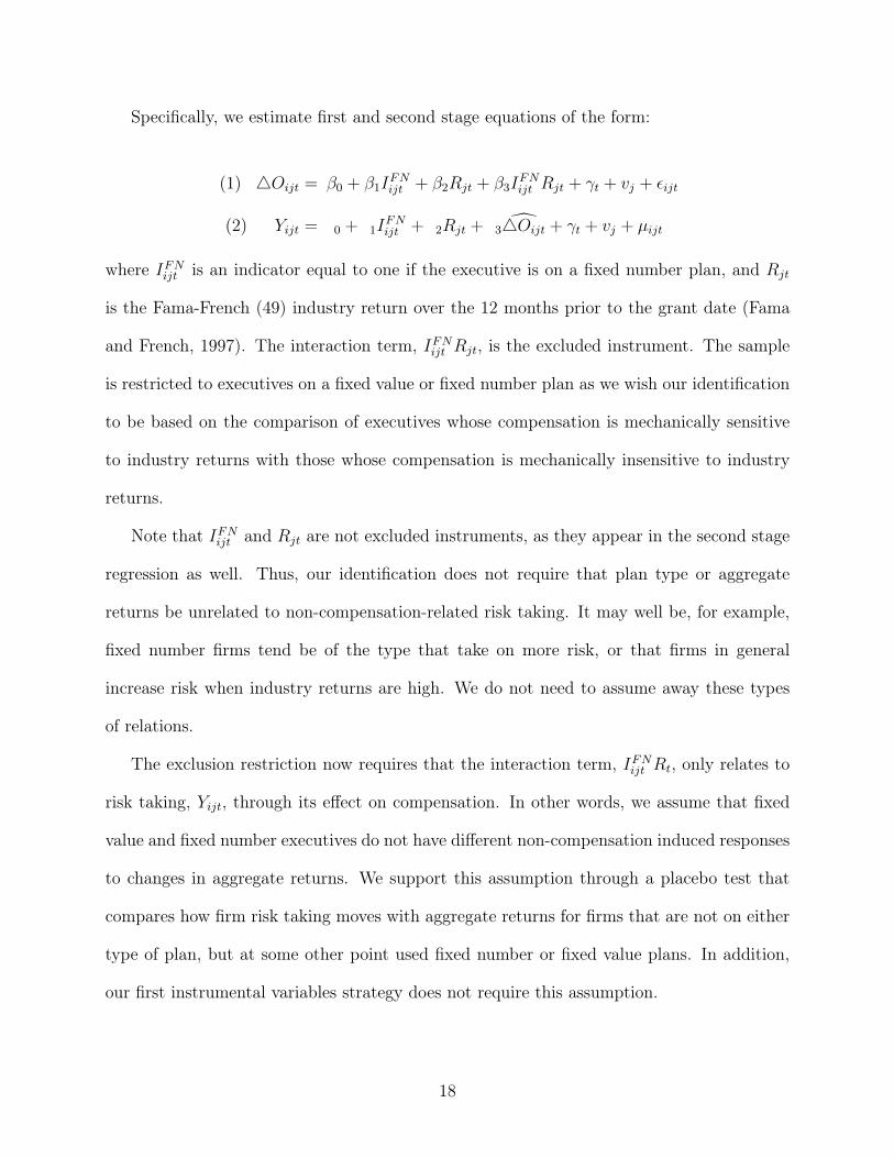
Specifically, we estimate first and second stage equations of the form:
j0 + j1IFN(1) 4O
ijt = ij t + j2Rjt + j3I
FN ij t Rjt + r
t + vj + ✏
ij t
1IFN(2) Y
ijt = 0 + + 2Rjt + 34Oij t + r
t + vj + µ
ij t ij t
d
where IFN is an indicator equal to one if the executive is on a fixed number plan, and Rjt
ij t
is the Fama-French (49) industry return over the 12 months prior to the grant date (Fama
and French, 1997). The interaction term, IFN Rjt
, is the excluded instrument. The sample ij t
is restricted to executives on a fixed value or fixed number plan as we wish our identification
to be based on the comparison of executives whose compensation is mechanically sensitive
to industry returns with those whose compensation is mechanically insensitive to industry
returns.
Note that IFN and Rjt are not excluded instruments, as they appear in the second stage
ij t
regression as well. Thus, our identification does not require that plan type or aggregate
returns be unrelated to non-compensation-related risk taking. It may well be, for example,
fixed number firms tend be of the type that take on more risk, or that firms in general
increase risk when industry returns are high. We do not need to assume away these types
of relations.
The exclusion restriction now requires that the interaction term, IFN Rt
, only relates to ij t
risk taking, Yij t , through its effect on compensation. In other words, we assume that fixed
value and fixed number executives do not have different non-compensation induced responses
to changes in aggregate returns. We support this assumption through a placebo test that
compares how firm risk taking moves with aggregate returns for firms that are not on either
type of plan, but at some other point used fixed number or fixed value plans. In addition,
our first instrumental variables strategy does not require this assumption.
18

3.3 Other Empirical Considerations
Before looking at the results, we address other important considerations that apply to both
strategies described above. First, both instruments directly affect changes in the value of
new options granted. However, few options vest in less than three years, i.e., they cannot
be exercised until three years after the grant date. Thus, the typical executive holds previ
ously granted options in addition to the new grant of options. This is not a problem for our
methodology because our instruments affect one component of total options held and have
no direct effect on the other components, so the instruments should also generate exogenous
variation in the total stock of options. While data on each executive’s total value of unex
ercised options is unavailable prior to 2006, we can approximate these values using the fact
that firms are required to report the total number of shares of unexercised exercisable and
unexercised unexercisable options held by each executive at the end of each firm fiscal year.
Our estimation procedure follows Core and Guay (2002). In unreported results, we show
that our instrument generates significant variation in the total value of an executive’s stock
of unexercised options. Importantly, this suggests that our results measure a lower bound.
Holding the stock of unexercised options constant, an exogenous 10 percent increase in the
value of a new option grant increases risk by 3 to 6 percent. If all options grants were to
increase by 10 percent, the effect on risk would likely be larger.
A second consideration relates to the fact that non-option based compensation may adjust
to offset changes in the value of options granted. For example, we know that in years when
the aggregate return is high, executives on fixed number cycles tend to experience increases
in option grants while those of fixed value cycles do not gain. During these boom periods,
boards may increase the non-option compensation (e.g. cash bonus) of fixed value executives
so that their total pay remains comparable to the total pay of fixed number executives. In
Section 4.4, we show that this effect does not seem to be significant in the data. However,
19
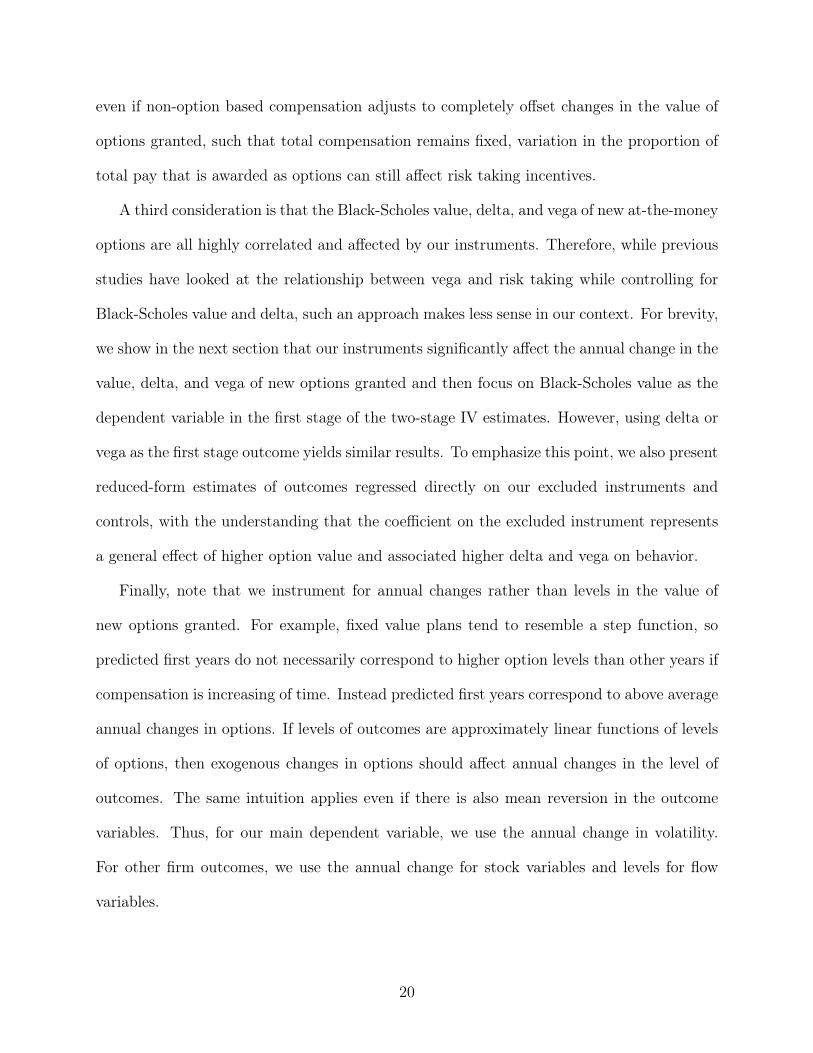
even if non-option based compensation adjusts to completely offset changes in the value of
options granted, such that total compensation remains fixed, variation in the proportion of
total pay that is awarded as options can still affect risk taking incentives.
A third consideration is that the Black-Scholes value, delta, and vega of new at-the-money
options are all highly correlated and affected by our instruments. Therefore, while previous
studies have looked at the relationship between vega and risk taking while controlling for
Black-Scholes value and delta, such an approach makes less sense in our context. For brevity,
we show in the next section that our instruments significantly affect the annual change in the
value, delta, and vega of new options granted and then focus on Black-Scholes value as the
dependent variable in the first stage of the two-stage IV estimates. However, using delta or
vega as the first stage outcome yields similar results. To emphasize this point, we also present
reduced-form estimates of outcomes regressed directly on our excluded instruments and
controls, with the understanding that the coefficient on the excluded instrument represents
a general effect of higher option value and associated higher delta and vega on behavior.
Finally, note that we instrument for annual changes rather than levels in the value of
new options granted. For example, fixed value plans tend to resemble a step function, so
predicted first years do not necessarily correspond to higher option levels than other years if
compensation is increasing of time. Instead predicted first years correspond to above average
annual changes in options. If levels of outcomes are approximately linear functions of levels
of options, then exogenous changes in options should affect annual changes in the level of
outcomes. The same intuition applies even if there is also mean reversion in the outcome
variables. Thus, for our main dependent variable, we use the annual change in volatility.
For other firm outcomes, we use the annual change for stock variables and levels for flow
variables.
20
4 Results
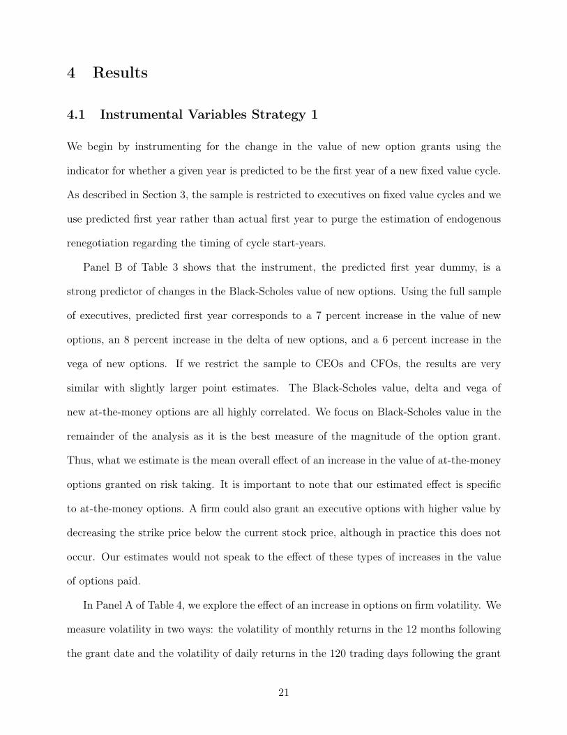
4.1 Instrumental Variables Strategy 1
We begin by instrumenting for the change in the value of new option grants using the
indicator for whether a given year is predicted to be the first year of a new fixed value cycle.
As described in Section 3, the sample is restricted to executives on fixed value cycles and we
use predicted first year rather than actual first year to purge the estimation of endogenous
renegotiation regarding the timing of cycle start-years.
Panel B of Table 3 shows that the instrument, the predicted first year dummy, is a
strong predictor of changes in the Black-Scholes value of new options. Using the full sample
of executives, predicted first year corresponds to a 7 percent increase in the value of new
options, an 8 percent increase in the delta of new options, and a 6 percent increase in the
vega of new options. If we restrict the sample to CEOs and CFOs, the results are very
similar with slightly larger point estimates. The Black-Scholes value, delta and vega of
new at-the-money options are all highly correlated. We focus on Black-Scholes value in the
remainder of the analysis as it is the best measure of the magnitude of the option grant.
Thus, what we estimate is the mean overall effect of an increase in the value of at-the-money
options granted on risk taking. It is important to note that our estimated effect is specific
to at-the-money options. A firm could also grant an executive options with higher value by
decreasing the strike price below the current stock price, although in practice this does not
occur. Our estimates would not speak to the effect of these types of increases in the value
of options paid.
In Panel A of Table 4, we explore the effect of an increase in options on firm volatility. We
measure volatility in two ways: the volatility of monthly returns in the 12 months following
the grant date and the volatility of daily returns in the 120 trading days following the grant
21

date (approximately half a year). Both are annualized. Because we use an instrument that
predicts changes in option value, we focus on annual changes in our volatility measure as
the outcome.6 The top panel presents the second stage of the IV regression of the change in
volatility on the change in the log Black-Scholes value of new option grants, as instrumented
by the predicted first year dummy. The bottom panel presents the reduced-form regression
of the change in volatility on the instrument and other controls. In all specifications, for
both the full sample and the subsample of CEOs and CFOs, we find that an increase in
options leads to an increase in equity volatility.
The results imply that a 10 percent increase in the value of new options corresponds to a
more than 0.02 unit increase in equity volatility relative to the median 0.3, or a 6.7 percent
increase in volatility. We can also consider the direct impact of the increase in volatility
on the executive’s wealth. The median executive in our sample holds options with a vega
of $100K. For an increase in volatility of 0.02, this translates to an additional $200K in
expected wealth.
In the remainder of the analysis we explore possible channels that may drive the change in
volatility. One prime candidate is leverage. Basic capital structure theory implies that, hold
ing the assets and real activity of the firm constant, an increase in leverage will mechanically
lead to an increase in equity volatility.
Panel B of Table 4 shows that an increase in options does indeed lead to significant
increases in leverage. A 10 percent increase in the value of new options corresponds to an
0.007 unit increase in the debt to capital ratio. Similarly, a 10 percent increase in the value
of new options corresponds to a 0.006 increase in the debt to asset ratio, a 6 percent increase
relative to the median.
Next, we explore the effect of options on investment. These tests should be viewed
6In unreported results, we also find a significant positive effect of an increase in options on the level of volatility.
22

as exploratory because it is not obvious how an increase in investment should affect firm
risk. Since we use exogenous variation in options rather than investment, we do not take
any position on the relationship between investment and risk. Instead, we explore how
option grants affect investment, and leave the question of whether this increase in investment
contributed to the observed increase in volatility to future work. In Panel A of Table 5, we
find that a 10 percent increase in options leads to a significant 1.7 percent increase in capital
expenditures and a 3 percent increase in total investment (defined as the sum of capital
expenditures, R&D, acquisitions, and advertising expenses).
Panel A of Table 5 also explores the effect of options on dividends. Column (3) shows that,
among firms that already pay dividends, a 10 percent increase in options leads to a significant
1.7 percent decline in dividends. The effect of options on the infra-marginal decision to pay
any dividends is also negative, although the magnitude of the effect is small and insignificant.
Again, we do not take a firm stand on how dividend payments affect firm risk. Nevertheless,
the analysis supports the validity of the instrumental variables methodology. We expect
that, all else equal, an increase in options should lead to lower dividend payments because
most executive stock options over the sample period are not dividend protected. Therefore,
while most equity holders should be indifferent to dividend policy, option holders gain from
reducing dividend payouts. The results in Table 5 using the instrument also stand in stark
contrast to the positive correlation between dividend growth and options as shown later
in Table A.1. The OLS results are likely driven by the problem that firms that are doing
well are likely to increase both dividends payouts and option payouts. This issue highlights
the necessity of the instrumental variables strategy draw out and clarify the true effects of
options on executive behavior.
Finally, Panel B of Table 5 shows that options lead to flat or negative changes in firm
performance. Equity returns in the 12 months following the increase in option grants are
23

flat, while measures of operating performance such as ROA and cash flow to assets are
significantly lower. However, we should not interpret the reduction in short term operating
performance as evidence that executives increase volatility at the cost of firm performance.
A short run decline in ROA or cash flows can also reflect a shift toward future oriented
projects that deliver back-loaded cash flows.
Altogether, these tables show that an increase in options leads to an increase in firm
volatility that is primarily driven by an increase in firm leverage. As discussed in detail
in Section 3 this analysis comes with three ma jor caveats. First, by using predicted first
year as our instrument, we rely on exogenously timed but expected increases in option pay.
Relative to random unexpected changes in options, this is a bias against our findings of a
positive changes in volatility. Second, we focus on exogenously timed changes in the value of
new option grants even though executives are likely to also be influenced by their total stock
of unexercised options, which includes unvested options granted in previous years. Finally,
we may be concerned that predicted first years will tend to coincide with turnover, product
cycles, or major performance reviews. Empirically, we find that expected cycle termination
is uncorrelated with turnover (see Section 4.4) and our conversations with compensation
consultants suggest that performance reviews are typically performed annually instead of at
cycle termination. However, we want to ensure that our results are robust to the possibility
that cycle termination is correlated with firm unobservables that may directly affect firm risk.
Therefore, in the next section we explore a second instrument for changes in option pay that
exploits variation in pay within cycles across executives rather than at cycle termination.
4.2 Instrumental Variables Strategy 2
We turn now to our second source of variation, which exploits the fact that the value of
options granted within fixed number cycles is more sensitive to market movements than the
24

value of options granted within fixed number cycles. Following the methodology described
in Section 3, the excluded instrument is the interaction between the fixed number indicator
and the industry return. The specification allows for endogenous fixed differences between
fixed number and fixed value executives and does not assume that plan type is randomly
assigned.
In Table 6, we show that the instrument indeed reliably predicts changes in the Black-
Scholes value, delta, and vega of new option grants. We find that, for a one standard
deviation change in the industry return, executives on fixed number plans receive an addi
tional 12 percent increase in option grants relative to executives on fixed value plans. Again
we instrument for changes in Black-Scholes value in the remainder of our analysis.
We begin using this second source of variation by exploring the effect of an increase in
options on changes in volatility, as measured by the 12 month volatility and the 120 trading
day volatility in the period after the option grant date. As with our first type of variation,
we present both the second stage of the IV specification and the reduced-form regression of
our outcome of interest on our instrument and controls. For brevity, Table 7 reports results
for the full sample of executives and clusters standard errors by firm to adjust for within-firm
correlations. Using this second source of variation, we again find that an increase in the value
of new option grants leads to an increase in equity volatility. The estimated magnitudes are
smaller, but not significantly different from those in the earlier estimation. A 10 percent
increase in the value of new options granted leads to an 0.007 increase in equity volatility,
or a 2.3 percent increase relative to median volatility.
We again find that the primary mechanism driving the change in volatility is an increase
in firm leverage. Columns (3) and (4) of Table 7 show that a 10 percent increase in the
value of new options granted leads to an approximately 3 percent increase in both the debt
to capital ratio and the debt to asset ratio.
25

Table 8 explores the effect of changes in options on investment, dividend policy, and firm
performance. The results are similar to those using the first source of variation, although
magnitudes differ slightly. We find that an increase leads to a marginally significant positive
increase in capital expenditures with noisily estimated effects for total investment. Dividend
growth falls significantly, which is consistent with the view that executives may wish to
lower dividends because many executive stock options are not dividend protected. Finally,
a increase in options leads to lower returns and operating performance (in contrast to the
results using the first instrument, here we estimate that the change is returns is marginally
significant while the change in operating performance as measured by ROA and cash flows is
noisily estimated). Overall, our second source of variation in option grants yields the same
message as before. Increased options lead to an increase in volatility that is primarily driven
by increases in leverage.
As described earlier, the validity of the second IV procedure rests upon the assumption
that fixed number and fixed value firms do not have differential non-compensation related
responses to changes in industry returns. If this assumption holds, then the observed changes
in volatility and other firm outcomes must be due to the change in option grants induced
by the differential sensitivity of fixed number plans to market movements. We support this
assumption by using a placebo test that compares the responses of fixed number and fixed
value firms to industry returns in years in which the firms do not award options according
to any multi-year plan. This placebo test exploits the fact that both fixed number and fixed
value cycles grew in popularity prior to the 2000s (due to the rise of options compensation
more generally) and fell in popularity after 2005, which is likely due to peer benchmarking
disclosure requirements that led to option grants being adjusted annually. We estimate the
following regression:
26

= j0 + j1IFN Placebo + j2Rit + j3I
FN Placebo Yij t
ij t ij t Rit + r
t + vj + ✏
ij t
We restrict the sample to executives who are, in some other year, on a fixed number or
fixed value cycle and we exclude those who have ever been on both types of cycles. IFN Placebo ij t
is an indicator for whether the executive was at some earlier or later point on a fixed number
cycle. A j3 close to zero would support the assumption that fixed number and fixed value
firms do not have different optimal responses to market movements.
Table 9 shows that, across a variety of outcome measures (change in option value, volatil
ity, return, investment, leverage, and dividend policy), fixed number and fixed value firms
react similarly to changes in industry returns in years in which the executive is not awarded
options according to either type of multi-year plan. It is further reassuring that the placebo
sample is similar in size to the IV sample and the point estimates are close to zero with small
standard errors, suggesting that j3 is a well-estimated zero effect. These results provide ev
idence of the differential responses of fixed number and fixed value firms to industry returns
in the years when options are awarded according to these cycles are due to the differential
sensitivity of their option compensation to these returns rather than other factors.
4.3 New vs. Existing Options
So far, we have reported the average effect of changes in the value of new option grants on
executive risk taking. In this section, we explore whether this effect varies with the total
amount of options held by the executive. We suspect that the effect of new options grants on
risk taking may be weaker if the executive already holds a large stock of unexercised options
that were granted in the past. Options are typically granted with a three-year minimum
vesting period, i.e., they cannot be exercised until three years after the grant date. While we
27

do not have precise measures of the Black-Scholes value, delta, or vega of each executive’s
stock of unexercised options, we can approximate these values using the fact that firms are
required to report the total number of shares of unexercised exerciseable and unexercised
unexerciseable options held by each executive at the end of each firm fiscal year. Our
estimation procedure follows Core and Guay (2002). We find that on average, new grants
account for one-fifth of the Black-Scholes value of all options held. Since new at-the-money
options tend to have higher vega than options that are already in-the-money, new option
grants account for a higher fraction of the vega of all unexercised options, approximately
one-third.
In Table 10 we find that the effect of increases in new option grants on changes in volatility
is two times larger if the the ratio of the value of new options to existing options is in the
upper half of the distribution. We find similar results when we divide the sample into terciles
in terms of the ratio of the value of new options to unexercised options.
As expected, we find that new options are more likely to affect behavior when they
significantly change an executive’s total option holdings. These results also suggest that our
estimates should be viewed as a lower bound. We measure the marginal change in behavior
following a shock to a single year of new option grants. If boards increase option grants in
all years, the changes in executive behavior are likely to be significantly larger.
4.4 Endogeneity
We exploit cycle-induced variation in option grants because we suspect that the correlation
between firm outcomes and option grants may be driven by other unobserved factors. In
Table A.1, we show the endogenous relationships between option grants and firm outcomes
as estimated using OLS. The top panel includes firm fixed effects while the bottom panel
28

excludes them.7 The OLS estimation leads to estimates that are very different, often of the
opposite sign, relative to those estimated using IV. Using OLS, an increase in option grants
is correlated with near zero changes in volatility and leverage, significant declines in firm
returns, and significant increases in investment and dividends. The results are suggestive of
strong endogeneity bias in the OLS estimation. For example, it may be the case that firms
that have done well in the past tend to increase options, and these firms also tend to have
relatively lower returns in the year following the pay raise relative to the high returns in the
previous year. Growth firms may tend to award more in options and engage in high levels
of investment. Finally, firms that have have done well may tend to increase both dividends
and option grants, resulting in a positive correlation between the two. This stands in sharp
contrast to the IV results, which find a negative causal relationship between options and
dividends, as predicted by the fact that most executive options are not dividend protected
and decline in value following dividend payments.
Table A.2 explores endogenous renegotiation of the terms of multi-year cycles and com
pensation. Endogenous renegotiation, to the extent that it occurs, does not bias our results
because we use predicted cycle status instead of actual cycle status as our first source of
variation and because we allow endogenous choice of fixed number or fixed value plans in
our second IV estimation. Nevertheless, we present supplementary results measuring the ex
tent of endogenous renegotiation. In Panel A, we explore whether executives tend to switch
between fixed number and fixed value plans (or depart from using any plan) depending on
firm or industry returns. We find very little evidence of endogenous switching between cycle
types. Even when the industry return is high, such that fixed value executives receiving less
pay that fixed number executives, fixed value executives are not more likely to depart from
7Because the outcomes are expressed in terms of changes or flows (investment is the change in capital stock), mean level differences across firms are already accounted for even in specifications without firm fixed effects. The addition of firm fixed effects controls for fixed differences in mean growth rates across firms.
29

their original cycle type. In Panel B we look at whether fixed value executives, in years
when the industry return is high, tend to receive raises in their non-option compensation to
compensate for the fact that their option compensation remains flat while other executives
likely receive increases in options. We find a positive but insignificant effect. Moreover,
even if it were the case that firms using fixed value plans adjusted other compensation so
that their executives’ total compensation were equally sensitive to aggregate returns as fixed
number executives, we would still expect risk taking to be less sensitive to aggregate returns
for fixed value executives. This follows because cash compensation does not create incentives
to take on risk. Finally, we test if the predicted termination of fixed value or fixed number
cycles tends to coincide with executive turnover and find no evidence of such effects.
5 Conclusion
We explore the effect of executive option grants on risk taking using two sources of variation
induced by the institutional features of multi-year grant cycles. First, the value of new
options grants increases by a large discrete amount in years that are predicted to be the
start of a new fixed value cycle. Second, fixed number executives receive option grants that
are more sensitive to market movements than fixed value executives.
The two types of variation yield similar results. We find that an increase in option
grants leads to a modest but significant increase in firm equity volatility. The ma jority of
this increase in volatility is driven by increases in leverage. An increase in option grants
also leads significantly lower dividend growth with mixed effects on investment and firm
performance.
30

References
Aggarwal, Rajesh K., and Andrew A. Samwick, 1999, The other side of the trade-off: The impact of risk on executive compensation, Journal of Political Economy 107, 65–105.
Agrawal, Anup, and Gershon N. Mandelker, 1987, Managerial incentives and corporate investment and financing decisions, The Journal of Finance 42, 823–837.
Berger, Philip G., Eli Ofek, and David L. Yermack, 1997, Managerial entrenchment and capital structure decisions, The Journal of Finance 52, 1411–1438.
Bettis, J. Carr, John Bizjak, Jeffrey Coles, and Swaminathan Kalpathy, 2012, Performance-vesting provisions in executive compensation, Working Paper.
Carpenter, Jennifer N., 2000, Does option compensation increase managerial risk appetite?, The Journal of Finance 55, 2311–2331.
Chava, Sudheer, and Amiyatosh Purnanandam, 2010, CEOs versus CFOs: incentives and corporate policies, Journal of Financial Economics 97, 263–278.
Cohen, Randolph B., Brian J. Hall, and Luis M. Viceira, 2000, Do executive stock options encourage risk-taking, Working Paper.
Core, John, and Wayne Guay, 1999, The use of equity grants to manage optimal equity incentive levels, Journal of Accounting and Economics 28, 151–184.
, 2002, Estimating the value of employee stock option portfolios and their sensitivities to price and volatility, Journal of Accounting Research 40, 613–630.
DeFusco, Richard A., Robert R. Johnson, and Thomas S. Zorn, 1990, The effect of executive stock option plans on stockholders and bondholders, The Journal of Finance 45, 617–627.
Denis, David J., Diane K. Denis, and Atulya Sarin, 1997, Agency problems, equity ownership, and corporate diversification, The Journal of Finance 52, 135–160.
Esty, Benjamin C., 1997, Organizational form and risk taking in the savings and loan industry, Journal of Financial Economics 44, 25–55.
Fama, Eugene F, and Kenneth R French, 1997, Industry costs of equity, Journal of Financial Economics 43, 153–93.
Frydman, Carola, and Dirk Jenter, 2010, CEO compensation, Annual Review of Financial Economics 2, 75–102.
Gormley, Todd A., David A. Matsa, and Todd T. Milbourn, 2012, CEO compensation and corporate risk-taking: Evidence from a natural experiment, SSRN eLibrary.
Guay, Wayne R., 1999, The sensitivity of ceo wealth to equity risk: An analysis of the magnitude and determinants, Journal of Financial Economics 53, 43–71.

Hall, Brian J., 1999, The design of multi-year stock option plans, Journal of Applied Corpo
rate Finance 12, 97–106.
Haugen, Robert A., and Lemma W. Senbet, 1981, Resolving the agency problems of external capital through options, The Journal of Finance 36, 629–647.
Hayes, Rachel M., Michael Lemmon, and Mingming Qiu, 2012, Stock options and managerial incentives for risk taking: Evidence from FAS 123R, Journal of Financial Economics 105, 174–190.
Knopf, John D., Jouahn Nam, and John H. Thornton, 2002, The volatility and price sensitivities of managerial stock option portfolios and corporate hedging, The Journal of Finance 57, 801–813.
Lambert, Richard A., David F. Larcker, and Robert E. Verrecchia, 1991, Portfolio considerations in valuing executive compensation, Journal of Accounting Research 29, 129–149.
Lewellen, Katharina, 2006, Financing decisions when managers are risk averse, Journal of Financial Economics 82, 551–589.
May, Don O., 1995, Do managerial motives influence firm risk reduction strategies?, The Journal of Finance 50, 1291–1308.
Mehran, Hamid, 1992, Executive incentive plans, corporate control, and capital structure, The Journal of Financial and Quantitative Analysis 27, 539–560.
Ross, Stephen A., 2004, Compensation, incentives, and the duality of risk aversion and riskiness, The Journal of Finance 59, 207–225.
Saunders, Anthony, Elizabeth Strock, and Nickolaos G. Travlos, 1990, Ownership structure, deregulation, and bank risk taking, The Journal of Finance 45, 643–654.
Schrand, Catherine, and Haluk Unal, 1998, Hedging and coordinated risk management: Evidence from thrift conversions, The Journal of Finance 53, 979–1013.
Smith, Clifford W., and Rene M. Stulz, 1985, The determinants of firms’ hedging policies, The Journal of Financial and Quantitative Analysis 20, 391–405.
Smith Jr., Clifford W., and Ross L. Watts, 1982, Incentive and tax effects of executive compensation plans, Australian Journal of Management (University of New South Wales) 7, 139.
Tufano, Peter, 1996, Who manages risk? an empirical examination of risk management practices in the gold mining industry, The Journal of Finance 51, 1097–1137.
Xu, Moqi, 2011, The costs and benefits of long-term ceo contracts, Working Paper.

Figure 1 Prevalence of Multi-Year Plans Over Time
This figure illustrates the prevalence of multi-year plans over time. The area under the bottom curve represents the percent of executives that were on a fixed-number plan, conditional on being paid options that year. The area between the top and bottom curves represents the percent of executives that were on a fixed-value plan. The years 1991 and 1992 are missing due to lack of data coverage.
0 10
20
30
40
50
60
Pe
rcen
t
1985 1990 1995 2000 2005 2010 Year
Fixed Number Fixed Value

Figure 2 Real Examples of Fixed Value Cycles and Predictions
This figure represents two examples of fixed value cycles taken from the data. Years that we predict to be cycle start years are indicated by a dotted vertical line.
Panel A: Example 1
150
200
250
300
350
Gra
nt V
alue
(Tho
usan
ds)
2004 2005 2006 2007 2008 2009 Year
Panel B: Example 2
0 20
0 40
0 60
0 G
rant
Val
ue (T
hous
ands
)
1998 1999 2000 2001 2002 2003 2004 2005 Year

Ta b l e 1 Length of Cycles
This table shows the distribution of cycle length by cycles type as well as pooled.
Fixed Number Fixed Value Total
Freq Pct Freq Pct Freq Pct
2 12449 68.73 35809 83.16 48258 78.88 3 3586 19.80 4978 11.56 8564 14.00 4 1183 6.53 1407 3.27 2590 4.23 5 495 2.73 435 1.01 930 1.52
� 6 401 2.21 433 1.01 834 1.36
Total 18114 100.00 43062 100.00 61176 100.00

Ta b l e 2 Firm Characteristics
This table shows firm characteristics by cycle type. Panel A shows the industry distribution for firms-years, broken down by the type of plan the CEO was on. Industries are categorized using the Fama-French 12 industry classification scheme. Panel B compares other firm characteristics across cycle types. Because there are likely to be time trends in these accounting variables, we take three cross sections of the data rather than pool all years.
Panel A: Industry Distribution
Fixed Number Fixed Value
Freq Pct Freq Pct
Consumer NonDurables 386 6.05 592 6.22 Consumer Durables 199 3.12 331 3.48 Manufacturing Oil, Gas, and Coal Chemicals
861 231 195
13.48 3.62 3.05
1,343 406 407
14.10 4.26 4.27
Business Equipment Communication
1,091 156
17.09 2.44
1,313 219
13.79 2.30
Utilities 229 3.59 429 4.50 Wholesale, Retail Healt h
726 678
11.37 10.62
983 875
10.32 9.19
Finance Other
1,028 605
16.10 9.48
1,702 924
17.87 9.70
Total 6,385 100.00 9,524 100.00
Panel B: Accounting Variables Year=1995
Fixed Number Fixed Value
Mean Median Mean Median
Assets 4440.84 1046.80 3952.22 1043.88 Sales 3167.94 1255.15 3079.98 1077.47 Market to Book 1.86 1.46 1.86 1.58 Firm Return 0.29 0.27 0.25 0.18 Options Compensation CAPX / PPE CAPX / Assets Debt to Capital Long-term Debt Total Dividends
799.77 0.32 0.09 0.37
903.71 92.90
410.49 0.21 0.07 0.37
194.30 6.87
723.06 0.31 0.10 0.36
736.12 85.38
442.52 0.24 0.08 0.36
180.10 11.20
Dividend Dummy 0.62 1.00 0.73 1.00

Ta b l e 2 (continued)
Year=2000
Fixed Number Fixed Value
Mean Median Mean Median
Assets 4714.24 900.11 5234.34 1308.48 Sales 3170.67 882.60 3817.95 1164.55 Market to Book 2.34 1.45 2.16 1.48 Firm Return 0.17 0.08 0.15 0.05 Options Compensation 3133.89 1064.21 2855.51 1220.67 CAPX / PPE 0.47 0.26 0.34 0.22 CAPX / Assets 0.08 0.05 0.08 0.06 Debt to Capital 0.36 0.34 0.36 0.37 Long-term Debt 986.67 198.44 1123.65 225.32 Total Dividends 110.66 0.00 88.01 2.82 Dividend Dummy 0.39 0.00 0.54 1.00
Year=2005
Fixed Number Fixed Value
Mean Median Mean Median
Assets 4440.84 1046.80 3952.22 1043.88 Sales 3167.94 1255.15 3079.98 1077.47 Market to Book 1.86 1.46 1.86 1.58 Firm Return 0.29 0.27 0.25 0.18 Options Compensation CAPX / PPE CAPX / Assets Debt to Capital Long-term Debt Total Dividends
799.77 0.32 0.09 0.37
903.71 92.90
410.49 0.21 0.07 0.37
194.30 6.87
723.06 0.31 0.10 0.36
736.12 85.38
442.52 0.24 0.08 0.36
180.10 11.20
Dividend Dummy 0.62 1.00 0.73 1.00

Ta b l e 3 Option Grants and Fixed Value First Years
Panel A of this table shows how option compensation changes in the first year of a fixed value cycle. Panel B shows how option compensation changes in predicted first years of a fixed value cycle. Observations are at the executive-year level. The sample is limited to executives on fixed value cycles. First year is an indicator variable equal to one if it is the first year of a fixed value cycle (or the year following the last year of a cycle). Predicted first year is an indicator variable equal to one if the year is predicted to be a first year based on the length of the previous cycle. The variable B-S Value equals the Black-Scholes value of options, Delta equals the change in Black-Scholes value associated with a 1 percent change in the price of the underlying, and Vega equals the change in Black-Scholes value associated with a .01 change in the annualized volatility of the underlying. Standard errors are clustered by firm to account for the fact that we observed multiple executives from the same firm.
Panel A: Real First Years
� Log B-S Value � Log Delta � Log Vega
(1) (2) (3) (4) (5) (6)
First Year 0.0596⇤⇤⇤ 0.0545⇤⇤⇤ 0.0518⇤⇤⇤ 0.0460⇤⇤⇤ 0.0381⇤⇤⇤ 0.0277⇤⇤
[8.33] [5.72] [7.55] [5.05] [4.22] [2.34]
Year FE Yes Yes Yes Yes Yes Yes Firm FE Yes Yes Yes Yes Yes Yes CEO/CFO Sample No Yes No Yes No Yes N 37378 15509 36649 15214 36649 15214 R2 0.107 0.0727 0.0930 0.0649 0.161 0.141
Panel B: Predicted First Years
� Log B-S Value � Log Delta � Log Vega
(1) (2) (3) (4) (5) (6)
Predicted First Year 0.0715⇤⇤⇤ 0.0760⇤⇤⇤ 0.0774⇤⇤⇤ 0.0824⇤⇤⇤ 0.0564⇤⇤⇤ 0.0579⇤⇤⇤
[7.92] [6.23] [8.85] [6.94] [5.34] [4.10]
Year FE Yes Yes Yes Yes Yes Yes Firm FE Yes Yes Yes Yes Yes Yes CEO/CFO Sample No Yes No Yes No Yes N 37378 15509 36649 15214 36649 15214 R2 0.107 0.0743 0.0950 0.0680 0.162 0.143

Ta b l e 4 IV1 - Volatility & Leverage
Panel A shows the IV and reduced form results for volatility, where �Log B-S Value is instrumented for by the Predicted First indicator, as defined in Table 3. Observations are at the executive-year level. The sample is limited to executives on fixed value cycles. We measure volatility in two ways: the annualized volatility of monthly returns in the 12 months following the grant date and the annualized volatility of daily returns in the 120 trading days following the grant date (approximately half of one year). Panel B shows the IV and reduced form results for leverage.
Panel A: Volatility
� 12 Month Volatility � 120 TD Volatility
(1) (2) (3) (4)
� Log B-S Value 0.211⇤⇤⇤ 0.247⇤⇤⇤ 0.192⇤⇤⇤ 0.218⇤⇤⇤
[5.10] [4.38] [5.00] [4.34]
Year FE Yes Yes Yes Yes Firm FE Yes Yes Yes Yes CEO/CFO Sample No Yes No Yes N 36558 14950 36562 14961 F-stat 65.87 40.12 66.04 41.07
� 12 Month Volatility � 120 TD Volatility
(1) (2) (3) (4)
Predicted First 0.0155⇤⇤⇤ 0.0181⇤⇤⇤ 0.0149⇤⇤⇤ 0.0173⇤⇤⇤
[6.41] [5.56] [6.72] [5.88]
Year FE Yes Yes Yes Yes Firm FE Yes Yes Yes Yes CEO/CFO Sample No Yes No Yes N 41268 16542 41248 16543 R2 0.257 0.225 0.267 0.231
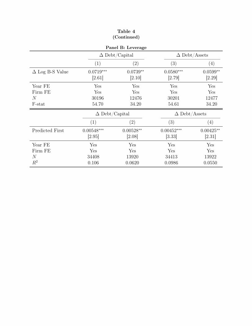
Ta b l e 4 (Continued)
Panel B: Leverage
� Debt/Capital � Debt/Assets
(1) (2) (3) (4)
� Log B-S Value 0.0719⇤⇤⇤ 0.0739⇤⇤ 0.0580⇤⇤⇤ 0.0599⇤⇤
[2.61] [2.10] [2.79] [2.29]
Year FE Yes Yes Yes Yes Firm FE Yes Yes Yes Yes N 30196 12476 30201 12477 F-stat 54.70 34.20 54.61 34.20
� Debt/Capital � Debt/Assets
(1) (2) (3) (4)
Predicted First 0.00548⇤⇤⇤ 0.00528⇤⇤ 0.00452⇤⇤⇤ 0.00425⇤⇤
[2.95] [2.08] [3.33] [2.31]
Year FE Yes Yes Yes Yes Firm FE Yes Yes Yes Yes N 34408 13920 34413 13922 R2 0.106 0.0620 0.0986 0.0550

Ta b l e 5 IV1 - Investment, Dividends, and Firm Performance
Panel A shows the IV and reduced form results for investment and dividends, where �Log B-S Value is instrumented for by the Predicted First indicator, as defined in Table 3. Observations are at the executive-year level. The sample is limited to executives on fixed value cycles. Investment is defined as capital expenditures or as total investment, which is the sum of capital expenditures, R&D, acquisitions, and advertising expenses. Panel B shows the IV and reduced form results for performance, which is measured using the stock return in the 12 months following the grant date, the return on assets and the cash flow-to-assets ratio.
Panel A: Investments and Dividends
Log CapX Log Total Inv � Log Dividends � Dividend Payer
(1) (2) (3) (4)
� Log B-S Value 0.171⇤ 0.295⇤⇤ -0.171⇤⇤ -0.0113 [1.80] [2.26] [-2.23] [-0.31]
Year FE Yes Yes Yes Yes Firm FE Yes Yes Yes Yes N 29707 29996 16774 30304 F-stat 54.76 57.27 48.78 55.21
Log CapX Log Total Inv � Log Dividends � Dividend Payer
(1) (2) (3) (4)
Predicted First 0.0161⇤⇤ 0.0275⇤⇤⇤ -0.0130⇤⇤ -0.000850 [2.28] [2.93] [-2.12] [-0.33]
Year FE Yes Yes Yes Yes Firm FE Yes Yes Yes Yes N 33855 34234 18773 34533 R2 0.924 0.856 0.261 0.0872

Ta b l e 5 (Continued)
Panel B: Firm Performance
12 Month Return ROA Cash Flow/Assets
(1) (2) (3)
� Log B-S Value -0.0910 -0.0535⇤⇤⇤ -0.0548⇤⇤⇤
[-1.01] [-3.14] [-2.81]
Year FE Yes Yes Yes Firm FE Yes Yes Yes CEO/CFO Sample No No No N 36763 30148 27623 F-stat 63.56 54.78 40.36
12 Month Return ROA Cash Flow/Assets
(1) (2) (3)
Predicted First -0.00470 -0.00335⇤⇤⇤ -0.00292⇤⇤⇤
[-0.72] [-3.05] [-2.63]
Year FE Yes Yes Yes Firm FE Yes Yes Yes CEO/CFO Sample No No No N 41822 34404 31453 R2 0.250 0.667 0.689

Ta b l e 6 IV2 - Differential Sensitivity to Industry Returns
This table shows the differential sensitivity of the compensation of fixed number and fixed value executives to industry returns. Observations are at the executive-year level. The sample is limited to executives that are either on fixed number of fixed value plans (not in their first year). The variable FN is an indicator equal to one if the executive is on a fixed number plan. Industry returns are defined the Fama-French (49) industry return of the executives’ firm in the 12 months preceding the option grant associated with the cycle. Other variables are defined as in Table 3. Main effects are included in the regressions but not shown. Standard errors are clustered by firm.
� Log B-S Value � Log Delta � Log Vega
(1) (2) (3)
FN ⇥ Ind Return 0.482⇤⇤⇤ 0.512⇤⇤⇤ 0.452⇤⇤⇤
[14.11] [15.50] [8.33]
Year FE Yes Yes Yes Firm FE Yes Yes Yes N 23352 22860 22860 R2 0.249 0.233 0.292

Ta b l e 7 IV2 - Volatility and Leverage
This table shows the IV and reduced form results for volatility and leverage, where �Log B-S Value is instrumented for by FN ⇥ Ind Return as defined in Table 6. Observations are at the executive-year level. The sample is limited to executives that are either on fixed number of fixed value plans (not in their first year). All other variables are as define in Table 4.
� 12 Month Vol � 120 TD Vol � Debt/Capital � Debt/Assets
(1) (2) (3) (4)
� Log B-S Value 0.0672⇤⇤ 0.0657⇤⇤ 0.0609⇤⇤⇤ 0.0311⇤⇤
[2.04] [2.05] [3.12] [2.19]
Year FE Yes Yes Yes Yes Firm FE Yes Yes Yes Yes N 22592 22565 18784 18788 F-stat 192.2 192.3 188.3 188.1
� 12 Month Vol � 120 TD Vol � Debt/Capital � Debt/Assets
(1) (2) (3) (4)
FN x Ind Return 0.0317⇤⇤ 0.0307⇤⇤ 0.0304⇤⇤⇤ 0.0159⇤⇤
[2.02] [2.04] [3.14] [2.23]
Year FE Yes Yes Yes Yes Firm FE Yes Yes Yes Yes N 23144 23114 19262 19266 R2 0.323 0.339 0.181 0.188

Ta b l e 8 IV2 - Investment, Dividends and Performance
This table shows the IV and reduced form results for Investment, Dividends and Performance, where �Log B-S Value is instrumented for by FN ⇥ Ind Return as defined in Table 6. Observations are at the executive-year level. The sample is limited to executives that are either on fixed number of fixed value plans (not in their first year). All other variables are as define in Table 5.
Panel A: Investment and Dividends
Log CapX Log Total Inv � Log Dividends � Dividend Payer
(1) (2) (3) (4)
� Log B-S Value 0.184⇤ -0.00325 -0.239⇤⇤ -0.0484 [1.72] [-0.03] [-2.00] [-1.63]
Year FE Yes Yes Yes Yes Firm FE Yes Yes Yes Yes N 18492 18673 10023 18855 F-stat 185.1 184.2 59.28 186.4
Log CapX Log Total Inv � Log Dividends � Dividend Payer
(1) (2) (3) (4)
FN x Ind Return 0.0877 -0.00718 -0.0860⇤⇤ -0.0253⇤
[1.64] [-0.12] [-2.16] [-1.73]
Year FE Yes Yes Yes Yes Firm FE Yes Yes Yes Yes N 18965 19153 10211 19331 R2 0.922 0.855 0.329 0.167

Ta b l e 8 (Continued)
Panel B: Firm Performance
12 Month Ret ROA Cash Flow/Assets
(1) (2) (3)
� Log B-S Value -0.175⇤ -0.00926 -0.0136 [-1.93] [-0.70] [-0.94]
Year FE Yes Yes Yes Firm FE Yes Yes Yes N 22709 18776 17173 F-stat 196.6 184.6 171.5
12 Month Ret ROA Cash Flow/Assets
(1) (2) (3)
FN x Ind Return -0.0826⇤ -0.00604 -0.00855 [-1.86] [-0.92] [-1.18]
Year FE Yes Yes Yes Firm FE Yes Yes Yes N 23304 19252 17618 R2 0.298 0.716 0.731

Ta b l e 9 Placebo Test
This table shows the reduced form results for outcomes from Tables 6-8 using a placebo sample of executive-years that were not on a fixed number or fixed value plan, but were associated with firms that at some point used (or would use in the future) one (but not both) of those types of plans. FN Placebo is an indicator variable equal to one of the the firm at some point used (or would use in the future) a fixed number plan, but was not currently.
� Log B-S Value � 12 Month Volatility 12 Month Return
(1) (2) (3)
FN Placebo x Ind Return -0.0497 0.0110 -0.0261 [-0.70] [0.72] [-0.61]
Year FE Yes Yes Yes Firm FE Yes Yes Yes N 14006 19400 22617 R2 0.0917 0.278 0.240
Log Total Inv � Debt/Capital � Log Dividends
(1) (2) (3)
FN Placebo x Ind Return 0.00733 0.00104 -0.0247 [0.16] [0.11] [-0.62]
Year FE Yes Yes Yes Firm FE Yes Yes Yes N 19005 16686 8149 R2 0.842 0.136 0.320

Ta b l e 1 0 New vs. Existing Options
This table shows that the effect of new option grants on firm volatility is greater in cases in which the value of new at-the-money option grants is a large fraction of the value of the total stock of unexercised options held by the executive. We re-estimate the reduced form specifications from Tables 4 and 7, interacting our instruments with indicator variables for whether the observation corresponds to the top half or top two terciles in terms of the value of new options as a fraction of the value of all unexercised options. For brevity, we present the coefficients for the main interaction terms of interest. All direct and two-way interaction terms are included as controls.
� 120 TD Volatility
(1) (2) (3) (4)
Pred 1st Yr 0.0105⇤⇤⇤ 0.0107⇤⇤⇤
[3.83] [3.36] Pred 1st Yr x Top Half Frac B-S Value 0.0106⇤⇤
[2.53] Pred 1st Yr x Middle Tercile Frac B-S Value -0.000431
[-0.10] Pred 1st Yr x Top Tercile Frac B-S Value 0.0174⇤⇤⇤
[3.13] FN x Ind Return -0.0167 -0.0367
[-0.87] [-1.53] FN x Ind Ret x Top Half Frac B-S Value 0.100⇤⇤⇤
[3.69] FN x Ind Ret x Middle Tercile Frac B-S Value 0.0715⇤⇤
[2.41] FN x Ind Ret x Top Tercile Frac B-S Value 0.130⇤⇤⇤
[3.48]
Year FE Yes Yes Yes Yes Firm FE Yes Yes Yes Yes N 38189 38189 22508 22508 R2 0.264 0.265 0.269 0.271

Ta b
l e A
. 1
OLS
Endog
enou
s C
orre
lati
ons
Thi
s ta
ble
show
s th
e O
LS r
esul
ts o
f reg
ress
ing �
Log
B-S
Val
ue o
n va
rious
out
com
es in
the
full
sam
ple
of e
xecu
tives
. Pa
nel A
in
clud
esfi r
mfi x
ed e
ff ect
s, w
hile
the
bot
tom
pan
el in
clud
es t
hem
.
Pan
el A
: Fir
m F
ixed
Eff
ects
� 1
2M V
ol
12M
Ret
urn
Log
Tota
l Inv
�
Deb
t/C
apita
l �
Log
Div
iden
ds
(1)
(2)
(3)
(4)
(5)
� L
og B
-S V
alue
0.
0030
6⇤
-0.0
302⇤
⇤⇤
0.02
24⇤⇤
⇤ -0
.005
74⇤⇤
⇤ 0.
0274
⇤⇤⇤
[1.6
8]
[-6.1
7]
[3.5
6]
[-4.8
6]
[5.5
9]
Year
FE
Yes
Yes
Yes
Yes
Yes
Firm
FE
Ye
s Ye
s Ye
s Ye
s Ye
s N
65
572
6594
0 54
477
5496
4 28
388
R
2 0.
245
0.21
9 0.
846
0.08
73
0.23
2
Pan
el B
: N
o Fir
m F
ixed
Eff
ects
� 1
2M V
ol
12M
Ret
urn
Log
Tota
l Inv
�
Deb
t/C
apita
l �
Log
Div
iden
ds
(1)
(2)
(3)
(4)
(5)
� L
og B
-S V
alue
-0
.002
77⇤⇤
⇤ -0
.018
4⇤⇤⇤
0.
608⇤
⇤⇤
0.00
0141
0.
0221
⇤⇤⇤
[-5.6
0]
[-8.3
0]
[33.
83]
[0.2
9]
[7.9
8]
Year
FE
Yes
Yes
Yes
Yes
Yes
Firm
FE
N
o N
o N
o N
o N
o N
79
886
8842
3 72
430
6666
7 33
854
R2
0.21
2 0.
122
0.24
8 0.
0168
0.
0482

Ta b
l e A
. 2
Endog
enou
s R
eneg
otia
tion
In
Pan
el A
, we
expl
ore
whe
ther
exe
cutiv
es t
end
to s
witc
h be
twee
n fi x
ed n
umbe
r an
d fi x
ed v
alue
pla
ns (
or d
epar
t fr
om u
sing
any
plan
) de
pend
ing
on fi
rm o
r in
dust
ry r
etur
ns.
In P
anel
B w
e lo
ok a
t w
heth
er fi
xed
valu
e ex
ecut
ives
, in
yea
rs w
hen
the
indu
stry
ret
urn
is hi
gh,
tend
to
rece
ive
raise
s in
the
ir no
n-op
tion
com
pens
atio
n to
com
pens
ate
for
the
fact
tha
t th
eir
optio
n co
mpe
nsat
ion
rem
ains
fl at
whi
le o
ther
exe
cutiv
es li
kely
rec
eive
incr
ease
s in
opt
ions
.
Pan
el A
: Sw
itch
ing
of C
ycle
Typ
e an
d R
eturn
s
FV t
o N
on-C
ycle
FV
to
FN
FN t
o N
on-C
ycle
FN
to
FV
(1)
(2)
(3)
(4)
Firm
Ret
urn
0.00
568
-0.0
0211
0.
0096
3 0.
0071
0 [0
.58]
[-1
.02]
[0
.74]
[1
.47]
In
dust
ry R
etur
n -0
.003
97
0.00
531
-0.0
0375
0.
0062
1 [-0
.18]
[0
.94]
[-0
.13]
[0
.50]
Year
FE
Yes
Yes
Yes
Yes
Firm
FE
Ye
s Ye
s Ye
s Ye
s N
22
772
2277
2 12
102
1210
2 R
2 0.
0001
50
0.05
61
0.04
11
0.03
22
Pan
el B
: A
dju
stm
ent
of O
ther
Com
pen
sati
on for
Fix
ed V
alue
Exe
cuti
ves
� L
og (
Sala
ry +
Bon
us)
� L
og N
on-O
ptio
n C
omp
Turn
over
Nex
t Ye
ar
(1)
(2)
(3)
FV x
Ind
Ret
urn
0.04
14
0.03
56
[1.6
2]
[0.8
6]
Pre
dict
ed L
ast
Year
0.
0002
54
[1.1
1]
Year
FE
Yes
Yes
Yes
Firm
FE
Ye
s Ye
s Ye
s N
23
127
2337
8 32
168
R
2 0.
192
0.08
08
0.23
6

Ta b l e A . 3 Sensitivity to New Grants to Stock Price: Fixed Value vs Fixed Number
This is an example adapted from Hall (1999). It shows how the value and number of options granted move with a firms stock price with a fixed number and fixed value plan.
Stock price
Year 1 Grant Year 2 Grant Year 3 Grant
Plan 100 120 144
Fixed Value
Fixed Number
Value of Options
Number of Options
Value of Options
Number of Options
$1,000,000
28,128
$1,000,000
28,128
$1,000,000
23,440
$1,200,000
28,128
$1,000,000
18,752
$1,440,000
28,128 Note: The annual standard devation is assumed to be 32 percent, the risk-free rate is 6 percent, the dividend rate is 3 percent and the maturity is 10 years