swarm intelligence – w10: applications of threshold- based

Swarm Intelligence – W10:Applications of Threshold-

Based Algorithms and Introduction to Sensor

Networks

Outline• Applications of Threshold-Based

Algorithms– Computational examples– Embedded systems examples

• Introduction to Wireless Sensor Networks– Overview– Motivating applications– Taxonomy– Challenges– WSN and SI

An Example of the Application of a Variable Threshold Model to a Problem of Adaptive Task

Allocation

• Simulations are carried out on a grid with 5X5 zones

• 4 neighboring zones (no differentiation) are taken into account in the calculations; the boundary conditions are periodic (wrap around)

• 5 agents

The case of an express mail company

Application to a Problem of Adaptive Task Allocation

• Different task = different zone -> demand specific to each of the zones! Each agent has 5x5=25 different thresholds!

• Share some similarities with your lab problem

• At each iteration, the demand is increased by 50 units in each of 5 randomly selected zones.

• The agents are consulted in random order, and each agent i computes its probability Ti,j of responding to the demand coming from each zone j. Response is reactive (based on a stimulus and a threshold function) but probabilistic in this case.

• If no agent has responded within 5 consultations, the next iteration begins.

• When an agent responds to a demand, it will be unavailable for a time proportional to the distance between its current position and the zone to which it is moving.

• When an agent moves to a zone, the demand associated with that zone remains at 0 while it is there.

Simulation details


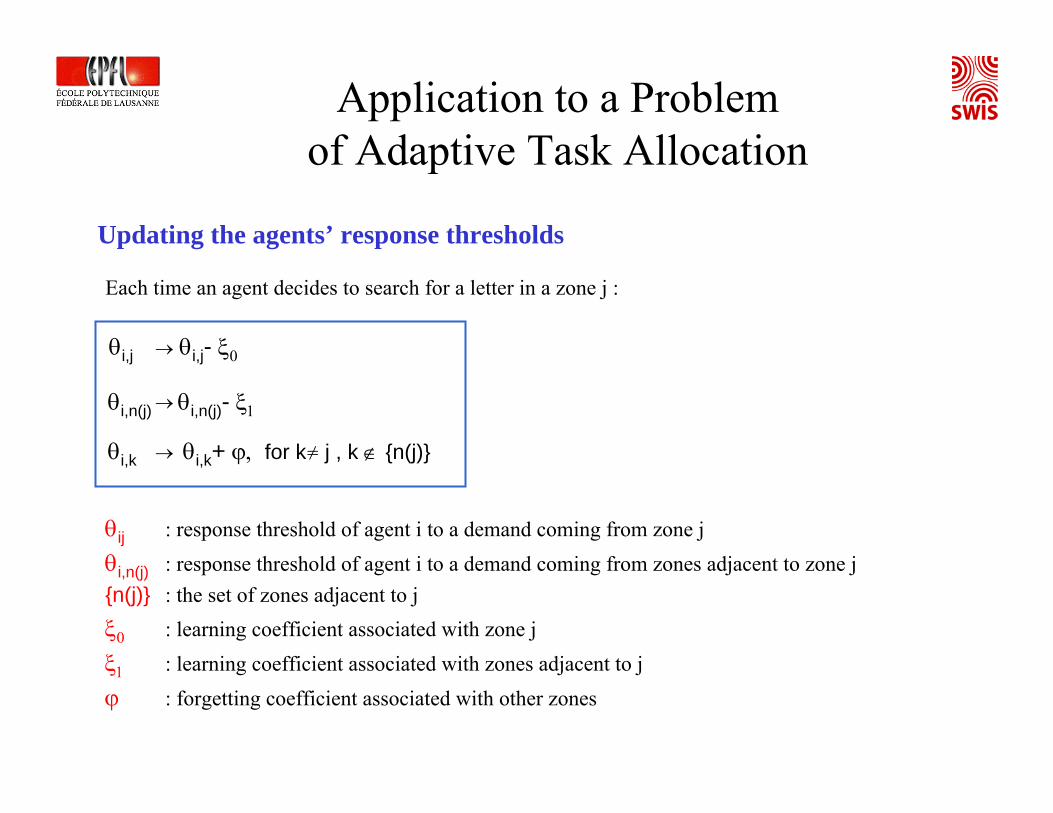
Each time an agent decides to search for a letter in a zone j :

θi,j θi,j- ξ0→

θi,n(j) θi,n(j)- ξ1→

θi,k θi,k+ ϕ, for k≠ j , k ∉ {n(j)}→

θij : response threshold of agent i to a demand coming from zone jθi,n(j) : response threshold of agent i to a demand coming from zones adjacent to zone j{n(j)} : the set of zones adjacent to jξ0 : learning coefficient associated with zone jξ1 : learning coefficient associated with zones adjacent to jϕ : forgetting coefficient associated with other zones

Updating the agents’ response thresholds


Tij : probability that an individual i, located in zone z(i) will respond to a demand sj in zone j

θi ∈ [θmin,θmax] : response threshold of agent i to a demand coming from zone jdz(i),j : distance between z(i) and jα ≥ 0, β ≥ 0 : modulation parameters

The threshold function

Tij(sj)= sj + αθij + βdz(i),j

sj2

2 2 2


Ex.1 β = 0 → standard threshold function; the higher threshold the higher needs to be thestimulus in order to respond (e.g. interest/laziness of the dispatcher for a given zone)Ex.2 α = 0 → response based only on the distance cost between demand in zone j and current zone z(i)

threshold

demand

specialist removal

Division of Labor in Robotic Systems Using Threshold-

Based Algorithms: Examples with one Task and One or

Multiple Castes

• 1 task: foraging (and maintaining nest reserves)

• Multiple castes (# of castes = # of robots): each of the robots is endowed with a different threshold

• Robot states: either active (foraging) or idle in the nest

• Foraging demand associated with a central stimulus: maintaining a virtual nest energy above a given level

• Foraging stimulus perceivable only in the nest; deterministic robot response

• Solution without com compared with primitive com (tandem recruitment)

The First Attempt to Transport a Threshold-Based Macroscopic Model to a Multi-Unit Embedded

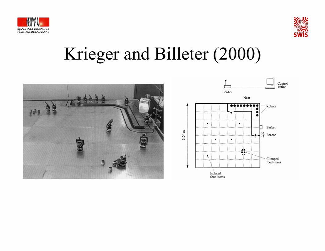
System (Krieger and Billeter, 2000)

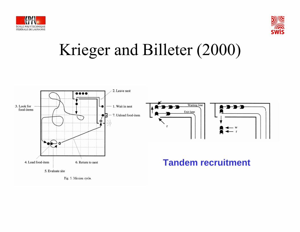
Krieger and Billeter (2000)


Tandem recruitment

Theoretical contribution

+ Fixed threshold algorithm verified in a real robot experiment+ Experimental sound results (10 runs per experiment, up to 12 robots, stat tests)- High investment in manpower (2.5 man/year) and hardware- No effort in exploiting the system noise in order to reduce individual

complexity; adapting macro-to-micro mechanisms to artificial platform- No effort to overcome unbalanced workload

- No systematic simulations, no modeling: isolated experiment.- No systematic study on threshold distribution and noise influence on response

Autonomous robotics contribution

- The experiment does not add any additional information to a simple macroscopic model since no effort on clarifying potential microscopic mechanisms

- No quantitative link between artificial (robots) and natural (ants) system

Social insect contribution (robots as a model for insects)


Threshold-Based Control of Aggregation Activity (Agassounon and Martinoli, 2001)

Special type of aggregation: linear structure building (more on week 13)

Initial situation Final situationParking lot

Controller without Threshold-Based Activity Regulation

Robot controller (FSM)

Note: obstacle avoidance/interference states in loaded and free conditions have to be separated for modeling purposes otherwise one of such maneuvers could induce a seed dropping/picking operation; at the real robot controller level the routine might be the same + load flag

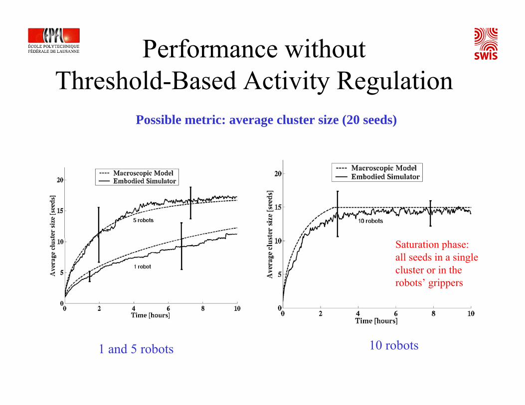
Possible metric: average cluster size (20 seeds)

1 and 5 robots 10 robots

Saturation phase: all seeds in a single cluster or in the robots’ grippers

Performance without Threshold-Based Activity Regulation

• Q: can we regulate the robot system activity in a fully distributed way so that robots the number of individuals active during the aggregation process is matched with aggregation demand?

• A: yes, using a threshold-based algorithm!

• Key motivations: – Evolution of manipulation sites: at the beginning there are several manipulation

sites, work in parallel positive; the more the aggregation/building process progresses the less manipulation sites there are, the more competition (interference) for the same manipulation sites there is.

– End criterion: a power-efficient building system should stop working when the task is accomplished

– Increasing the final cluster size: at the end all the seeds should belong to the single cluster (only those on the ground count for the aggregation metrics)

– Designing a truly distributed threshold-based algorithm (no supervisor!)

Distributed Activity Regulation of Aggregation?

• 1 task: aggregation → 1 threshold per robot • How many different thresholds, threshold distribution?• Ideas (minimizing complexity, maximizing robustness/interchangeability):

– Robots have the same capabilities, no reason to have different threshold– Probabilistic response even with a single threshold will suffice to regulate the activity;

not all the robots stop at the same time, when one drop the work, direct influence on aggregation demand

– How do we implement: deterministic response + noise = probabilistic response →exploit local perception based on on-board sensors as noise generator!

• Chosen stimulus: time needed to find a seed to manipulate; the larger the time, the lower the stimulus associated with the aggregation demand

• Special case of demand evolution: it does not increase automatically but stay constant if nothing is done. Initial condition: s(0) = S0 and δ = 0 (instead of s(0) = 0 δ > 0 as in the previous examples) → switching mechanism asymmetric: active → idle possible; idle → active not possible.

• Algorithm extensible with a random wake up time/…; customized to aggregation demand without major seed reinsertion

Implementation of the Threshold-Based Algorithm

20 seeds, threshold for abandoning the arena= 25 min, 1-5 robots

Average cluster size Number of active robots

Performance with Threshold-Based Activity Regulation

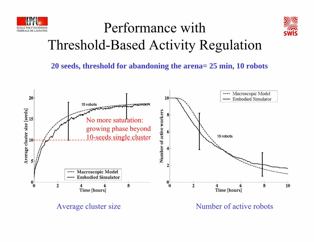
Average cluster size Number of active robots

No more saturation:growing phase beyond 10-seeds single cluster

Performance with Threshold-Based Activity Regulation20 seeds, threshold for abandoning the arena= 25 min, 10 robots

How good does this work?

Advantages– easy to determine, unique threshold for the all team;– robot homogenous (also controller): on average good load distribution– optimal value determined as a function of the system feature (number of

robots/speed/number of seeds/arena surface etc. ) → quantitative models (micro and macro) can help to find the optimal threshold

Drawbacks– fixed unique threshold = single parameter encoding the whole dynamics of the

experiment → algorithm extremely robust but system operation point might be sub-optimal in case of major environmental changes (e.g., double the aggregation area) or system changes (e.g., half of the robots fail)

– parameter difficult to tune analytically if noise distribution non parametric (e.g. no assumption on the distribution possible)

Example of Performance LandscapeThreshold optimization with macroscopic model (numerical integration)

Optimal threshold = 27 min for a given cluster size at a given time

Robots stop to early

Robots still keep working and keep the seedsIn their grippers

• PrFT: Threshold-based algorithm with private demand estimation and fixedthresholds; algorithms of the previous slides

• PrVT: variable threshold; not continuously adapting but calibration phase, then fixed threshold → result in a heterogeneous, multi-caste group

• PuFT: fixed threshold but demand estimated via wireless sharing among all members (average)

• PuVT: variable threshold (calibration) + demand estimation shared

• Arena 1: standard arena (that of previous slides), 80x80 cm, 20 seeds• Arena 2: larger arena, 178x178 cm, 20 seeds• Arena 3: standard arena, 20 seeds, 5 seeds added after 2 hours into the

aggregation process

Robots are not Ants: Can we exploit Wireless Com for Demand Estimation?

NOTE: com only used for stimulus estimation sharing; no central decision making as in market-based approaches!!!

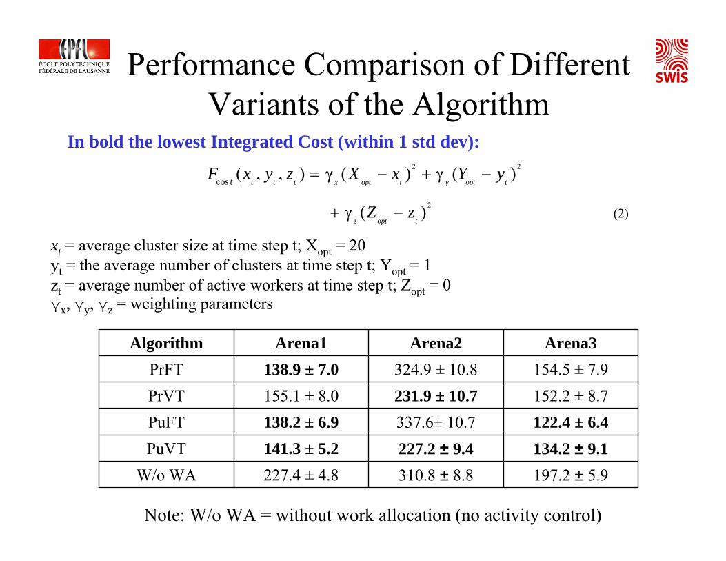
In bold the lowest Integrated Cost (within 1 std dev):

197.2 ± 5.9310.8 ± 8.8227.4 ± 4.8W/o WA134.2 ± 9.1227.2 ± 9.4141.3 ± 5.2PuVT122.4 ± 6.4337.6± 10.7138.2 ± 6.9PuFT152.2 ± 8.7231.9 ± 10.7155.1 ± 8.0PrVT154.5 ± 7.9324.9 ± 10.8138.9 ± 7.0PrFT

Arena3Arena2Arena1Algorithm

2 2

2

cos

(2)

( , , ) γ ( ) γ ( )

γ ( ) t t t x opt t y opt t

z opt t

tF x y z X x Y y

Z z

= − + −

+ −

Note: W/o WA = without work allocation (no activity control)

xt = average cluster size at time step t; Xopt = 20yt = the average number of clusters at time step t; Yopt = 1zt = average number of active workers at time step t; Zopt = 0 γx, γy, γz = weighting parameters

Performance Comparison of Different Variants of the Algorithm

An Introduction to Sensor Networks

Selected Slides from MOBICOM 2002 Tutorial T5

Wireless Sensor NetworksDeborah Estrin & Mani [email protected], [email protected]

UCLA

Akbar [email protected]

University of Wisconsin, MadisonCopyright © 2002

Intro

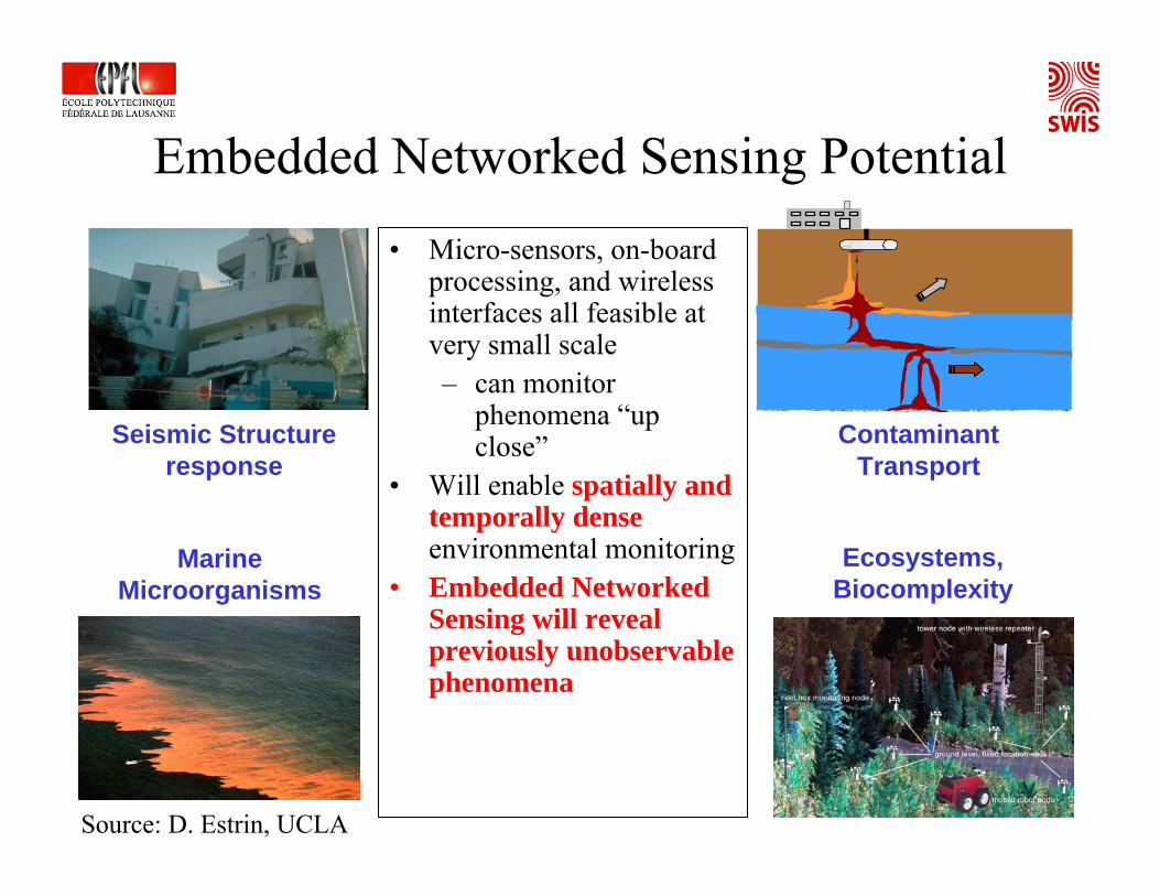
Embedded Networked Sensing Potential• Micro-sensors, on-board

processing, and wireless interfaces all feasible at very small scale– can monitor

phenomena “up close”

• Will enable spatially and temporally denseenvironmental monitoring

• Embedded Networked Sensing will reveal previously unobservable phenomena

Seismic Structure response

Contaminant Transport

Marine Microorganisms

Ecosystems, Biocomplexity

Source: D. Estrin, UCLA

Motivating Applications

App#1: Seismic• Interaction between ground motions and

structure/foundation response not well understood.– Current seismic networks not spatially

dense enough to monitor structure deformation in response to ground motion, to sample wavefield without spatial aliasing.

• Science– Understand response of buildings and

underlying soil to ground shaking – Develop models to predict structure response

for earthquake scenarios.• Technology/Applications

– Identification of seismic events that cause significant structure shaking.

– Local, at-node processing of waveforms.– Dense structure monitoring systems.

• ENS will provide field data at sufficient densities to develop predictive models of structure, foundation, soil response.Source: D. Estrin, UCLA

Field Experiment

⎜⎯⎯⎯⎯⎯⎯⎯ 1 km ⎯⎯⎯⎯⎯⎯⎜

• 38 strong-motion seismometers in 17-story steel-frame Factor Building.• 100 free-field seismometers in UCLA campus ground at 100-m spacing


Research challenges• Real-time analysis for rapid response.• Massive amount of data → Smart, efficient, innovative data

management and analysis tools.• Poor signal-to-noise ratio due to traffic, construction,

explosions, …. • Insufficient data for large earthquakes → Structure

response must be extrapolated from small and moderate-size earthquakes, and force-vibration testing.

• First steps– Monitor building motion – Develop algorithm for network to recognize significant seismic events

using real-time monitoring.– Develop theoretical model of building motion and soil structure by

numerical simulation and inversion.– Apply dense sensing of building and infrastructure (plumbing, ducts) with

experimental nodes.Source: D. Estrin, UCLA

App#2: Contaminant Transport• Science

– Understand intermedia contaminant transport and fate in real systems.

– Identify risky situations before they become exposures. Subterranean deployment.

• Multiple modalities (e.g., pH, redox conditions, etc.)

• Micro sizes for some applications (e.g., pesticide transport in plant roots).

• Tracking contaminant “fronts”.• At-node interpretation of

potential for risk (in field deployment).

Soil Zone

Groundwater

Volatization

SpillPath

Air Emissions

Dissolution

Water Well


Contaminantplume

ENS Research Implications

• Environmental Micro-Sensors– Sensors capable of

recognizing phases in air/water/soil mixtures.

– Sensors that withstand physically and chemically harsh conditions.

– Microsensors.• Signal Processing

– Nodes capable of real-time analysis of signals.

– Collaborative signal processing to expend energy only where there is risk.Source: D. Estrin, UCLA

App#3:Ecosystem MonitoringScience• Understand response of wild populations (plants and animals) to habitats

over time.• Develop in situ observation of species and ecosystem dynamics.

Techniques• Data acquisition of physical and chemical properties, at various

spatial and temporal scales, appropriate to the ecosystem, species and habitat.

• Automatic identification of organisms(current techniques involve close-range human observation).

• Measurements over long period of time,taken in-situ.

• Harsh environments with extremes in temperature, moisture, obstructions, ...


WSN Requirements for Habitat/Ecophysiology Applications

• Diverse sensor sizes (1-10 cm), spatial sampling intervals (1 cm - 100 m), and temporal sampling intervals (1 ms -days), depending on habitats and organisms.

• Naive approach → Too many sensors →Too many data.– In-network, distributed information processing

• Wireless communication due to climate, terrain, thick vegetation.

• Adaptive Self-Organization to achieve reliable, long-lived, operation in dynamic, resource-limited, harsh environment.

• Mobility for deploying scarce resources (e.g., high resolution sensors).


Field Experiments • Monitoring ecosystem

processes– Imaging, ecophysiology, and

environmental sensors– Study vegetation response to

climatic trends and diseases.• Species Monitoring

– Visual identification, tracking, and population measurement of birds and other vertebrates

– Acoustical sensing for identification, spatial position, population estimation.

Vegetation change detection

Avian monitoring Virtual field observations


Enabling Technologies

Enabling Technologies

Embedded Networked

Sensing& Actuation

Control system w/Small form factorUntethered nodes

ExploitcollaborativeSensing, action

Tightly coupled to physical world

Embed numerous distributed devices to monitor and interact with physical world

Network devices to coordinate and perform higher-level tasks

Exploit spatially and temporally dense, in situ, sensing and actuation


Sensors & Actuators• Passive elements: seismic, acoustic, infrared, strain,

salinity, humidity, temperature, etc.

• Passive arrays: imagers (visible, IR), biochemical

• Active sensors: radar, sonar– High energy, in contrast to passive elements

• Actuators: TBD• Technology trend: use of IC technology for increased

robustness, lower cost, smaller size


Challenges

Sensor Node Energy Roadmap

20002000 20022002 20042004

10,00010,000

1,0001,000

100100

1010

11

.1.1

Ave

rage

Pow

er (m

W)

• Deployed (5W)

• PAC/C Baseline (.5W)

• (50 mW)

(1mW)

RehostingRehosting to Low to Low Power COTSPower COTS(10x)(10x)

--SystemSystem--OnOn--ChipChip--Adv Power Adv Power ManagementManagementAlgorithms (50x)Algorithms (50x)

Source: ISI & DARPA PAC/C Program

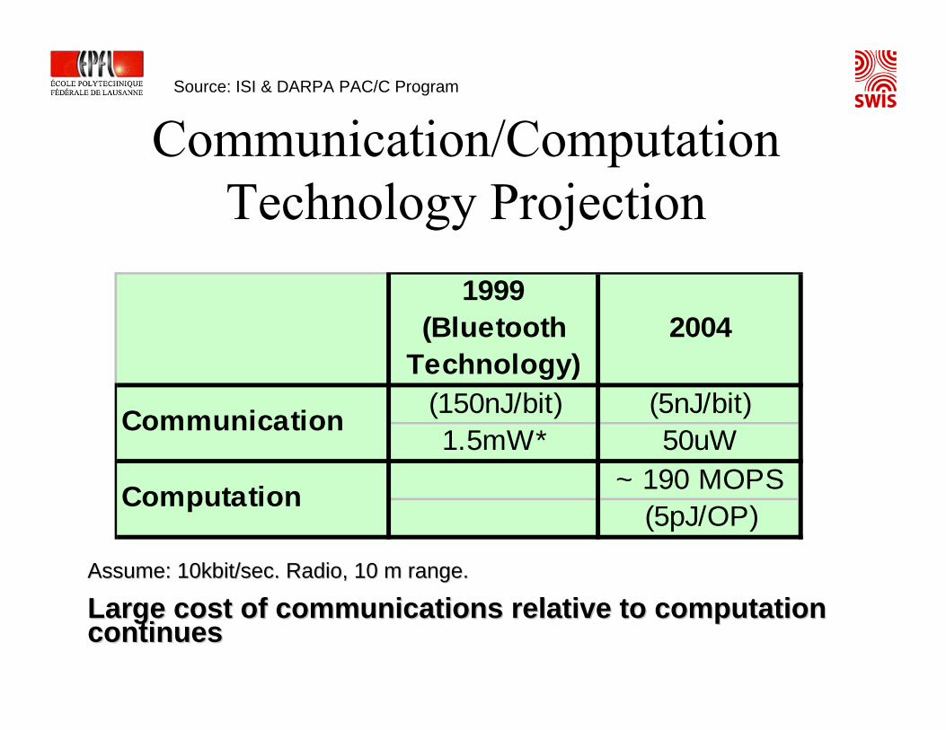
Communication/Computation Technology Projection

Assume: 10kbit/sec. Radio, 10 m range.Assume: 10kbit/sec. Radio, 10 m range.

Large cost of communications relative to computation Large cost of communications relative to computation continuescontinues

1999 (Bluetooth

Technology)2004

(150nJ/bit) (5nJ/bit)1.5mW* 50uW

~ 190 MOPS(5pJ/OP)

Computation

Communication

Source: ISI & DARPA PAC/C Program

New Design Themes• Long-lived systems that can be untethered and unattended

– Low-duty cycle operation with bounded latency– Exploit redundancy and heterogeneous tiered systems

• Leverage data processing inside the network– Thousands or millions of operations per second can be done using energy of

sending a bit over 10 or 100 meters (Pottie00)– Exploit computation near data to reduce communication

• Self configuring systems that can be deployed ad hoc– Un-modeled physical world dynamics makes systems appear ad hoc– Measure and adapt to unpredictable environment– Exploit spatial diversity and density of sensor/actuator nodes

• Achieve desired global behavior with adaptive localized algorithms– Cant afford to extract dynamic state information needed for centralized

control


From Embedded Sensing to Embedded Control

• Embedded in unattended “control systems”– Different from traditional Internet, PDA, Mobility applications – More than control of the sensor network itself

• Critical applications extend beyond sensing to control and actuation– Transportation, Precision Agriculture, Medical monitoring and

drug delivery, Battlefied applications– Concerns extend beyond traditional networked systems

• Usability, Reliability, Safety• Need systems architecture to manage interactions

– Current system development: one-off, incrementally tuned, stove-piped

– Serious repercussions for piecemeal uncoordinated design: insufficient longevity, interoperability, safety, robustness, scalability...


Sample Layered Architecture

Resource constraints call for more tightly integrated layers

Open Question:

Can we define anInternet-like architecture for such application-specific systems??

In-network: Application processing, Data aggregation, Query processing

Adaptive topology, Geo-Routing

MAC, Time, Location

Phy: comm, sensing, actuation, SP

User Queries, External Database

Data dissemination, storage, caching


Taxonomy of Applications and a few

Concrete Design Examples

• Spatial and Temporal Scale

– Extent– Spatial Density (of

sensors relative to stimulus)

– Data rate of stimulii• Variability

– Ad hoc vs. engineered system structure

– System task variability– Mobility (variability in

space)• Autonomy

– Multiple sensor modalities

– Computational model complexity

• Resource constraints– Energy, BW– Storage, Computation

Systems Taxonomy

• Frequency– spatial and

temporal density of events

• Locality – spatial, temporal

correlation• Mobility

– Rate and pattern

Load/Event Models

Metrics

• Efficiency– System

lifetime/System resources

• Resolution/Fidelity– Detection,

Identification• Latency

– Response time• Robustness

– Vulnerability to node failure and environmental dynamics

• Scalability– Over space and

time

Design Customization and Validation


Two Main Application Categories

C1: Low-duty cycle continuous sampling (e.g., temperature/humidity field monitoring over years)

C2: Event-based monitoring (e.g., human, animal species monitoring) → probably the most appropriate one for SI algorithms since collaboration in a dynamic environment emphasized

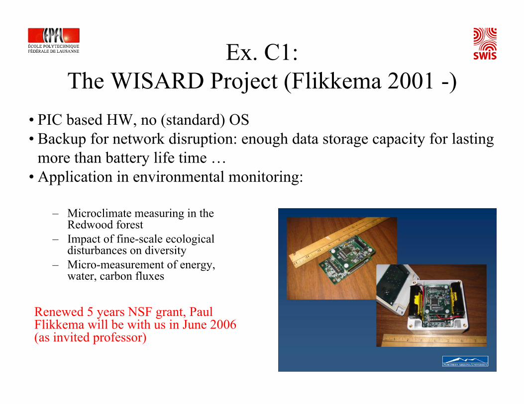
Ex. C1:The WISARD Project (Flikkema 2001 -)

– Microclimate measuring in the Redwood forest

– Impact of fine-scale ecological disturbances on diversity

– Micro-measurement of energy, water, carbon fluxes

• PIC based HW, no (standard) OS• Backup for network disruption: enough data storage capacity for lasting

more than battery life time …• Application in environmental monitoring:

Renewed 5 years NSF grant, Paul Flikkema will be with us in June 2006 (as invited professor)

Ex. C2: EPFL-UNILAvian Tracking Project

(Freitag, Martinoli, Urzelai, 1995-1999)

Goals • Understanding better the overall

behavior of migratory Wrynecks (endangered species) and therefore actively intervene for improving his survivability

• Monitoring nest passages, hunting movements, environmental cues (e.g., temperature inside and outside the nest)

EPFL-UNIL Avian ProjectOverview of the monitoring system

HMU

HMU

HMUHMU

HMU

HMUHMU HMU

HMUHMU

HMU

Hunting zone

≈ 200 m≈ 30 m

NMU

Nest

HMU = hunting monitoring unitNMU = nest monitoring unit

EPFL-UNIL Avian Tracking Project

Hunting Monitoring Unit• Active radio transponders (low

duty cycle)• RSSI-based distance estimation• No networking among HMU• Energy management based on

rough estimation of bird’s habits • Data collection with HP

calculator/laptop• Never tested in the field with

tagged wrynecks

EPFL-UNIL Avian Tracking ProjectNest Monitoring Unit• Passive Integrated Transponders (PIT), 16-

bit bound to animal’s leg• Energy management based on rough

estimation of bird’s habits and coupling of light barrier with PIT reader

• Male/female identification• Data collection with HP calculator/laptop • Tested in the field with tagged Wrynecks

[Freitag, Martinoli, Urzelai, Bird Study, 2001]

EPFL-UNIL Avian Tracking ProjectConclusion – Development and field experience• Extremely tough experience (1 month/year for testing the

equipment in the field with tagged Wrynecks; no failure admitted)• Birds do not usually play the game as we would like to

(camouflage, …) • Packaging: major issue (waterproof case, connectors, …)• Not low-stress monitoring (bird captured with nets, …); very

invasive technique but still … tagless techniques?• Wireless technology at that time very primitive.• At that time 1 week full autonomy: great! But networking and

collaboration could have allowed much better performances …• Much better than standard human-guided radio-telemetry • Full time job for having impact! (not in parallel to a PhD …)

Target Tracking using WSN

• Advantage of networking:– Allows for real-time collaboration → in-network

processing → more data acquired and only relevant, pre-processed data stored

– Energy saving: wake up only when needed (through prediction, load balancing)

– Centralized data gathering possible (sink)– Centralized network control possible (e.g., software

upgrade, reset, etc.)• Drawbacks:

– Increased power consumption– Increased node complexity

Tracking Challenges• Data dissemination and storage• Resource allocation and control• Operating under uncertainty• Real-time constraints• Data fusion (measurement interpretation)

• Multiple target disambiguation• Track modeling, continuity and prediction• Target identification and classification

Tracking Domains• Appropriate strategy depends on the sensors’

capabilities, domain goals and environment– Requires multiple measurements?– Bounded communication?– Target movement characteristics?– No single solution for all problems

• For example…– Limited bandwidth encourages local processing– Limited sensors requires cooperation

Why Not Centralized Tracking?

• Scale!• Data processing combinatorics• Resource bottleneck (communication, processing)• Single point of failure• Ignores benefits of locality

Why Not (fully) Distributed Tracking? (i.e. everyone tracks)

• Redundant information and computation• Can increase uncertainty• Lack of unified view • High communication costs

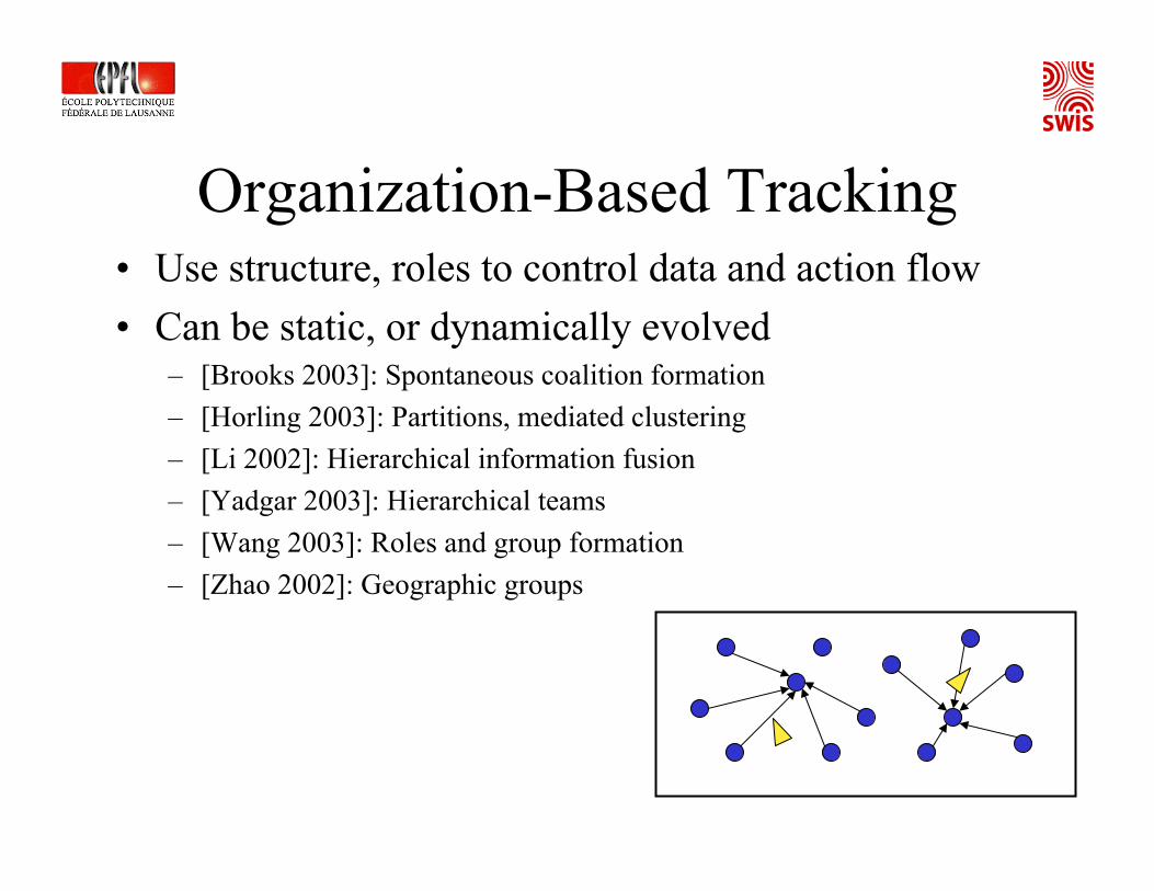
Organization-Based Tracking• Use structure, roles to control data and action flow• Can be static, or dynamically evolved

– [Brooks 2003]: Spontaneous coalition formation– [Horling 2003]: Partitions, mediated clustering– [Li 2002]: Hierarchical information fusion– [Yadgar 2003]: Hierarchical teams– [Wang 2003]: Roles and group formation– [Zhao 2002]: Geographic groups

Routing and Information Flow Management in WSN

– IP-based protocol not suited (different from traditional wireless networks, S-D ID matter)

– Two approaches: data-centric and location-centric– Data-centric: publish/subscribe architecture based n

data characteristic (e.g. Directed Diffusion routing algorithm, Estrin)

– Location-centric: geographic cells plays the role of nodes in IP networks (e.g., UW-routing, Ramanathan)

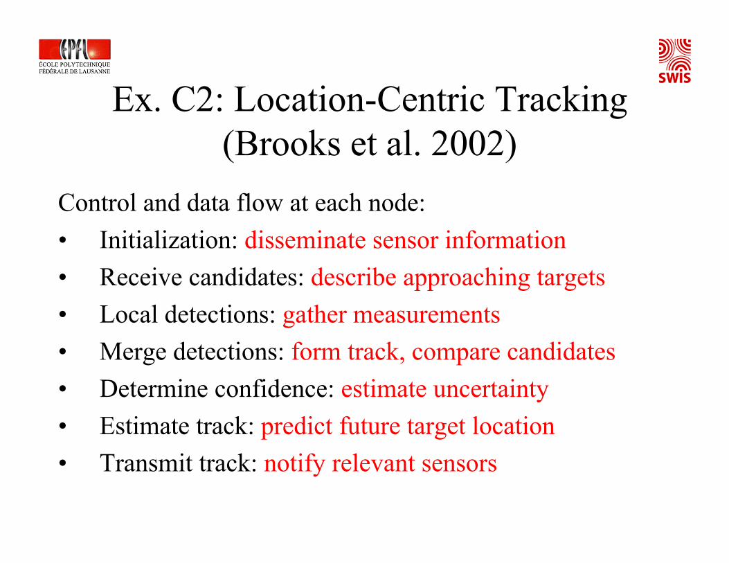
Control and data flow at each node:• Initialization: disseminate sensor information• Receive candidates: describe approaching targets• Local detections: gather measurements• Merge detections: form track, compare candidates• Determine confidence: estimate uncertainty• Estimate track: predict future target location• Transmit track: notify relevant sensors

Ex. C2: Location-Centric Tracking (Brooks et al. 2002)

Location-Centric Tracking• “Closest point of approach” (CPA) measurements• Target detection causes cell formation

– Cells formed around the target’s estimated location– Intended to include relevant sensors– Several modalities (e.g. acoustic, IR, etc.)

• Manager is selected– Node with greatest signal

strength• Manager collects local CPA’s

– Linear regression over CPA node locations

Location-Centric Tracking

• Estimated location compared to prior tracks– Projections from candidate tracks

• Cell created for track in new area– Size is a function of target velocity– Track information propagated to cell

• Tracking repeats…

Results (Brooks et al, 2002)

No filtering Extended Kalman Filtering(assumption linear trajectory)

Lateral Inhibition(no assumption on target, wait time proportional goodness-of-fit)

Data association and Collaborative Signal Processing (Filtering): single target, 40 nodes deployed along a road

SI and Wireless Sensor Networks

WSN and SI• SI principles might have impact because:

– Volume/mass constraints and therefore limited resources at the individual node level

– Large number of nodes– Autonomy– Collaboration among nodes– Self-organization

• And might not have impact because:– Most of them assume underlying mobile systems– Most of them do not exploit direct communication– Most of them rely on full distributedness and often

centralization and synchronization means energy saving

WSN and SI

• WSN push for redefinition of SI, less bio-inspired• We have not clearly identified yet where self-

organization principles and SI-based algorithms can be competitive.

• You have played with a first attempt/toy example in the lab (threshold-based algorithm applied to load balancing in a monitoring task)

WSN vs. Robots as Demonstrators for SI

• Another type of distributed HW platform: usually static nodes but still sensing, computing, communicating, acting (?)

• Sensor node = mobile robot without wheel or mobile robot = sensor node with wheels?

• Mobility changes completely the picture of the problem: more unpredictability, noise, … .

• Self-locomotion even more so: real-time control loop at the node level + energy budget radically different

Pointers and Additional Literature

Pointers on WSN• Mobicom 02 tutorial:

http://nesl.ee.ucla.edu/tutorials/mobicom02/• Course list:

http://www-net.cs.umass.edu/cs791_sensornets/additional_resources.htm• TinyOS:

http://www.tinyos.net/• Smart Dust Project

http://robotics.eecs.berkeley.edu/~pister/SmartDust/• UCLA Center for Embedded Networking Center

http://www.cens.ucla.edu/• Intel research Lab at Berkeley

http://www.intel-research.net/berkeley/• NCCR-MICS at EPFL and other Swiss institutions

http://www.mics.org

Additional Literature – Week 10Papers• Campos M., Bonabeau E., Theraulaz G., and Deneubourg J.-L.,

“Dynamic Scheduling and Division of Labor in Social Insects”, Adaptive Behavior, 2001, Vol. 8, No. 2, pp. 83-92.

• Cicirello V. A. and Smith S. F. 2004. Wasp-like Agents for Distributed Factory Coordination. J. of Autonomous Agents and Multi-Agent Systems, 8(3): 237-266.

• Krieger M. J. B. and Billeter J.-B., “The Call of Duty: Self-OrganisedTask Allocation in a Population of up to Twelve Mobile Robots”. Robotics and Autonomous Systems, 2000, Vol. 30, No. 1-2, pp. 65-84.

• Labella T. H., Dorigo M., and Deneubourg J.-L. 2004. Efficiency and Task Allocation in Prey Retrieval. In Ijspeert A. J. and Murata M., editors, Proc. First Int. Workshop on Biologically Inspired Approaches to Information Technology, Lausanne, Switzerland, Lecture Notes in Computer Sciences, pp. 32-47.

swarm intelligence – w10: applications of threshold- based

Documents