svclassify: a method to establish benchmark structural ... · biorxiv preprint first posted online...

svclassify: a method to establish benchmark structural variant calls

Hemang Parikh1,2, Hariharan Iyer3, Desu Chen4, Mark Pratt5, Gabor Bartha5, Noah Spies1,6,

Wolfgang Losert4, Justin M. Zook1*, Marc L. Salit1,7*

1Genome-Scale Measurements Group, National Institute of Standards and Technology,

Gaithersburg, MD 20899, USA.

2Dakota Consulting Inc., 1110 Bonifant Street, Suite 310, Silver Spring, MD 20910, USA.

3Statistical Engineering Division, National Institute of Standards and Technology, Gaithersburg,

MD 20899, USA.

4Institute for Research in Electronics and Applied Physics, University of Maryland, College

Park, MD 20742, USA.

5Personalis Inc., 1350 Willow Road, Suite 202, Menlo Park, CA 94025, USA.

6Department of Pathology, Stanford University, Stanford, CA, USA.

7Bioengineering Department, Stanford University, Stanford, CA, USA.

*These authors have contributed equally to this work

Corresponding author:

Justin M. Zook

Genome-Scale Measurements Group

Biosystems and Biomaterials Division

National Institute of Standards and Technology

100 Bureau Dr, MS8313,

Gaithersburg, MD 20899

USA

E-mail: [email protected]

.CC-BY 4.0 International licensepeer-reviewed) is the author/funder. It is made available under aThe copyright holder for this preprint (which was not. http://dx.doi.org/10.1101/019372doi: bioRxiv preprint first posted online May. 16, 2015;

http://dx.doi.org/10.1101/019372

http://creativecommons.org/licenses/by/4.0/

Abstract

The human genome contains variants ranging in size from small single nucleotide polymorphisms

(SNPs) to large structural variants (SVs). High-quality benchmark small variant calls for the pilot

National Institute of Standards and Technology (NIST) Reference Material (NA12878) have

recently been developed by the Genome in a Bottle Consortium, but no similar high-quality

benchmark SV calls exist for this genome. Since SV callers output highly discordant results, we

developed methods to combine multiple forms of evidence from multiple sequencing technologies

to classify candidate SVs into likely true or false positives. Our method (svclassify) calculates

annotations from one or more aligned bam files from any high-throughput sequencing technology,

and then builds a one-class model using these annotations to classify candidate SVs as likely true

or false positives. We first used pedigree analysis to develop a set of high-confidence breakpoint-

resolved large deletions. We then used svclassify to cluster and classify these deletions as well as

a set of high-confidence deletions from the 1000 Genomes Project and a set of breakpoint-resolved

complex insertions from Spiral Genetics. We find that likely SVs generally cluster separately from

likely non-SVs based on our annotations, and that the SVs cluster into different types of deletions.

We then developed a supervised one-class classification method that uses a training set of random

non-SV regions to determine whether candidate SVs have abnormal annotations different from

most of the genome. To test this classification method, we use our pedigree-based breakpoint-

resolved SVs, 1000 Genomes Project validated SVs validated by the 1000 Genomes Project, and

assembly-based breakpoint-resolved insertions, along with semi-automated visualization using

svviz. We find that candidate SVs with high scores are generally true SVs, and candidate SVs

with low scores are questionable. We distribute a set of 2676 high-confidence deletions and 68

high-confidence insertions with high svclassify scores from these call sets for benchmarking SV

callers.


http://dx.doi.org/10.1101/019372


Introduction

The human genome contains variants ranging in size from small single nucleotide

polymorphisms (SNPs) to large structural variants (SVs). SVs include variations such as novel

sequence insertions, deletions, inversions, mobile-element insertions, tandem duplications,

interspersed duplications and translocations. In general, SVs include deletions and insertions

larger than 50 base pairs (bps), while smaller insertions or deletions are referred to as indels, though

the threshold of 50 bps is somewhat arbitrary and based on the fact that different bioinformatics

methods are usually used to detect SVs vs. small indels and SNPs. SVs have long been implicated

in phenotypic diversity and human diseases [1]; however, identifying all SVs in a whole genome

with high-confidence has proven elusive. Recent advances in next-generation sequencing (NGS)

technologies have facilitated the analysis of SVs in unprecedented detail, but these methods tend

to give highly non-overlapping results [2]. In this work, we develop methods to evaluate candidate

SVs based on evidence from multiple NGS technologies.

NGS offers unprecedented capacity to detect many types of SVs on a genome-wide scale.

Many bioinformatics algorithms are available for detecting SVs using NGS including depth of

coverage (DOC), paired-end mapping (PEM), split-read and assembly-based methods [2]. DOC

approaches identify regions with abnormally high or low coverage as potential copy number

variants. Hence, DOC methods are limited to detecting only deletions and duplications but not

other types of SVs, and they have more power to detect larger events and deletions. PEM methods

evaluate the span and orientation of paired-end reads. Read pairs map farther apart around

deletions and closer around insertions, and orientation inconsistencies indicate potential inversions

or tandem duplications. Split reads are used to identify SVs by identifying reads whose alignments

to the reference genome are split in two parts and contain the SV breakpoint. Assembly-based

methods first perform a de novo assembly, and then the assembled genome is compared to the

reference genome to identify all types of SVs. By combining various approaches to detect SVs, it

is possible to overcome the limitations of individual approaches in terms of the types and sizes of

SVs that they are able to detect, but still difficult to determine which are true [3, 4].

Numerous methods have been developed to find candidate SVs using NGS, but clinical

adoption of human genome sequencing requires methods with known accuracy. The Genome in

a Bottle Consortium (GIAB) is developing well-characterized whole-genome reference materials


http://dx.doi.org/10.1101/019372


for assessing variant-call accuracy and understanding biases. Recently GIAB released high-

confidence SNP, indel, and homozygous reference genotypes for Coriell DNA sample NA12878,

which is also National Institute of Standards and Technology (NIST) Reference Material 8398

available at https://www-s.nist.gov/srmors/view_detail.cfm?srm=8398 [5]. In this work, we

developed methods to integrate evidence of SVs in mapped sequencing reads from multiple

sequencing technologies. We used unsupervised machine learning to determine the characteristics

of the different SV types, and we used One Class Classification to classify candidate SVs as likely

true positives, false positives, or ambiguous. Using these methods, we classified three

independently established “validated” call sets containing large deletions or insertions.

Our classification methods use the machine learning technique One Class Classification

(OCC) [6, 7]. In contrast to the more common two-class models that have two training sets (e.g.,

positives and negatives), one-class methods have only a single training set and try to identify sites

unlike the training set. In our OCC methods, the algorithm tries to identify a region, R, of the

annotation space that contains a specified, large proportion (e.g. 95% or 99%) of the non-SVs.

Sites that have annotations falling outside R are classified as SVs. In essence, these are outliers

relative to the non-SVs. For selecting R, only a representative set of non-SVs is required for the

training. In our model, we use random genomic coordinates as our one class because random

coordinates are unlikely to be near true SV breakpoints. For our one-class model, we only include

annotations that are likely to indicate a SV if they differ from random coordinates for a defined set

of parameters (e.g., read clipping, pair distance, and coverage). We do not include annotations

like mapping quality that may not always distinguish SVs from non-SVs because atypical values

may also indicate random regions of the genome that are difficult to sequence. We do not use a

two class machine learning model because our potential training SV call sets are primarily easier-

to-detect mid-size deletions and insertions and are not representative of all types of deletions,

insertions, or other SV types, which is an important assumption of two-class models. Therefore,

a two class model trying to differentiate our SV sets from random genomic coordinates can do a

very good job separating these two sets, but the model is likely to misclassify other candidate SVs

not in the “Validated/assembled” call sets (e.g., duplications, deletions in difficult parts of the

genome, etc.). Because our one-class model does not rely on biased “Validated/assembled” call

sets, we expect our one-class model to be more generalizable to other types of SVs by selecting

annotations for which atypical values are usually associated with SVs. Our methods, which


https://www-s.nist.gov/srmors/view_detail.cfm?srm=8398

http://dx.doi.org/10.1101/019372


classify based on evidence from multiple technologies, are complementary to the recently

published Parliament method [8], which generates candidate SVs using multiple technologies and

bioinformatics methods, and then uses a PacBio/Illumina hybrid assembly to determine whether

the candidate SVs are likely to be true. Similarly, in the characterization of the performance of

the LUMPY tool, the authors developed a high-confidence set that had breakpoints supported by

long reads from PacBio or Moleculo. In addition to using svviz to visualize and determine the

number of reads supporting the alternate, we also combine the support from multiple sequencing

technologies in a robust machine learning model.


http://dx.doi.org/10.1101/019372


Materials and Methods

Data sets

Four whole-genome sequencing data sets (Table 1) were used to develop methods to classify

candidate SVs into true positives and false positives for Coriell DNA sample NA12878. Two data

sets were generated using short-read sequencing technologies, and two other data sets were

generated using long-read sequencing technologies. For the Platinum Genomes 2x100bps HiSeq

data, raw reads were mapped to the National Center for Biotechnology Information (NCBI) build

37 using the Burrows-Wheeler Aligner (BWA) software with default parameters [9]. For Illumina

HiSeq (read length = 250 bps), PacBio, and Moleculo whole-genome sequencing data sets, aligned

bam files were publicly available and were used directly in this study.

SV validated/assembled sets

Three validated/assembled SV sets (Table 2) totaling 5,035 deletions and 70 insertions were

derived from Coriell DNA sample NA12878.

(A) Personalis deletions calls were derived based on pedigree analysis, which included 16

members of the family.

To be included in the validated/assembled set, the following conditions had to be met:

(1) Deletion must have been detected in at least one NA12878 sample.

(2) Deletion must have been detected in at least 2 other samples in the pedigree

with exact breakpoint matches.

The Personalis gold data set was further refined by experimental validations. Primers were

designed based on following criteria:

(1) Each primer maps no more than 3 times in genome.

(2) Require unique polymerase chain reaction (PCR) product in genome.

(3) 400 - 800 bps product size.

(4) Pad 100 bps around each deletion junction.


http://dx.doi.org/10.1101/019372


For small deletions (< 200 bps) a single primer pair was designed that straddled the

deletion. For large deletions (> 1500 bps) two primer pairs were designed around each

reference breakpoint junction. Site specific PCR amplification and high depth MiSeq

shotgun sequencing followed by manual inspection of the alignments was used to validate

all the deletions. Sanger sequencing was used when we were not able confirm the deletion

with MiSeq. For 3 deletions (2:104186941-104187136, 7:13022102-13028550, and

14:80106289-80115049) this was done because we did not see any junction reads.

(B) The 1000 Genomes Project validated/assembled contains the set of validation deletion calls

found in the genome of NA12878 by the 1000 Genomes Project pilot phase [10, 11]. These

deletion calls were validated by assembly or by other independent technologies such as array

comparative genomic hybridization, sequence capture array, superarray, or PCR.

(C) Spiral Genetics’ Anchored Assembly was performed whole read overlap assembly on

corrected, unmapped reads to detect structural variants using Illumina 2x100bps HiSeq whole-

genome sequencing data set. Sequencing errors were corrected by counting k-mers. Low count

k-mers were discarded as erroneous. The set of high scoring, or true k-mers was used to construct

a de Bruijn graph representing an error-free reconstruction of the true read sequences. Each read

was corrected by finding the globally optimum base substitution(s) so that it aligned to the graph

with no mismatches and differed by the smallest base quality score from the original read. Of

these corrected reads, those that did not match the reference exactly were assembled into a

discontiguous read overlap graph to capture sequence variation from the reference. Variants were

mapped to human reference coordinates (NCBI build 37) by walking the read overlap graph in

both directions until an “anchor” read, where a continuous 65 bps matches the reference, denoted

the beginning and end of each variant. Where a variant had more than one anchor, pairing

information was used to determine the correct location of the anchor. We used 70 calls from the

“Insertions” output, all of which were complex insertions (i.e., a set of reference bases was

replaced by a larger number of bases).

Deduplicated deletions


http://dx.doi.org/10.1101/019372


Any overlapping deletions within the validated/assembled SV sets were discarded, which resulted

in 2336 unique Personalis deletion calls and 1825 unique 1000 Genomes deletion calls (Table 2).

Bedtools’ intersect function was used to screen overlap between these two datasets

(Supplementary table 1). Merged deduplicated deletion calls were generated by keeping all the

2336 unique Personalis deletion calls and merging with 746 non-overlapping 1000 Genomes

deletion calls with minimum overlap required to be 1 bp, which resulted 3082 deduplicated

deletion calls.

Random region non-SV call sets

In addition, five sets of likely non-SVs were generated: 2 random and 3 from repetitive regions of

the genome (Table 2) as follows:

(1) 4000 random regions were generated with a uniform size distribution on a log scale from

50 bps to 997527 bps. Start sites were chosen randomly using the Generate Random

Genomic Coordinates script in R

(http://www.niravmalani.org/generate-random-genomic-coordinates/).

(2) 2306 random regions were generated with a size distribution matching the calls from the

pedigree-based Personalis deletions call set. Start sites were chosen randomly using the

Generate Random Genomic Coordinates script in R

(http://www.niravmalani.org/generate-random-genomic-coordinates/).

(3) 497 long interspersed nuclear elements (LINEs) were randomly selected from a list of

LINEs from the University of California, Santa Cruz (UCSC) Genome Browser’s

RepeatMasker Track.

(4) 498 long terminal repeat elements (LTRs) were randomly selected from a list of LTRs from

the UCSC Genome Browser’s RepeatMasker Track.

(5) 496 short interspersed nuclear elements (SINEs) were randomly selected from a list of

SINEs from the UCSC Genome Browser’s RepeatMasker Track.

svclassify


http://dx.doi.org/10.1101/019372


The svclassify tool was developed to quantify annotations of aligned reads inside and around each

SV (Figure 1). It was written using the Perl programming language employing SAMtools (version

0.1.19-44428cd) [12] and BEDTools (version 2.17.0) [13] to calculate parameters such as

coverage, paired-end distance, soft clipped reads, mapping quality, numbers of discordant paired-

ends reads, numbers of heterozygous and homozygous SNP genotype calls, percentage of the GC-

content, percentage of the repeats and low complexity DNA sequence bases, and mapping quality.

svclassify requires the following inputs: a BAM file of aligned reads, a list of SVs, homozygous

and heterozygous SNP genotype calls, a list of repeats from the UCSC Genome Browser’s

RepeatMasker Track and a reference genome. BAM files can come from any aligner. The user

can specify the size for the flanking regions. svclassify also includes partially mapped reads to the

L, LM, M, RM, or R regions for calculations. The insert size is calculated as the end-to-end

distance between the reads (length of both reads + distance separating the reads). Because PacBio

reads have high insertion and deletion error rates, Del (the mean of deleted bases of the reads) and

Ins (the mean of inserted bases of the reads) were normalized by subtracting the mean Del (0.0428)

and Ins (0.0948) per read length of 4000 random regions. For exploratory analyses, svclassify

generates 85 to 180 annotations for each SV from each dataset, depending on sequencing

technology (Supplementary table 2 and 3). For our unsupervised and one class analyses, we used

only subsets of these annotations that we expected to give the best results. These subsetted

annotations are given in the csv files (Supplementary table 4 to 7).

Data Analysis

The results from svclassify were subjected to two types of analyses – (1) Unsupervised Learning

based on a hierarchical cluster analysis using the L1 distance (also called Manhattan distance), and

(2) One Class Classification using the L1 distance or support vector machines (SVM) using a

carefully selected set of 4000 non-SVs.

Unsupervised Learning

Data values for each variable (characteristic) used in the analysis were first transformed using an

inverse hyperbolic sine transformation [14]. This transformation uses the following function.


http://dx.doi.org/10.1101/019372


y = sinh-1(x) = loge[x + sqrt(x2+1)]

This function is often used as an alternative to the logarithmic transformation. It has the advantage

that zero or negative values of x do not cause problems. Generally speaking it is quite similar to

a standard logarithmic transformation except near and below zero. Next, all variables were

standardized by subtracting the mean and dividing by the standard deviation. All further work was

done using these transformed data.

A hierarchical cluster analysis was performed with all 7797 random sites, 5035 deletion sites, and

70 insertion sites (see Table 2), using L1 distance as the distance function rather than Euclidean

distance [15] since Manhattan distance is less influenced by outliers within the non-SV class. The

Ward method was used for clustering [16]. A classical multidimensional scaling (MDS) analysis

was carried out to help visualize the spatial locations of the clusters [17]. For a given positive

integer k, the MDS algorithm determines a k-dimensional representation of the data space such

that the distances between pairs of data points in the original data space are preserved as best as

possible. We used k = 3 in our analysis to facilitate visualization. We used the

OneClassPlusSVM.R script.

One-class classification using L1 distance

The set of 4000 random sites representing the class of likely non-SVs with a size range of 50 bps

to 997527 bps were used for training the one-class classifier. First, a separate classifier was

developed using data from each sequencing technology for these 4000 sites. The classifier was

based on the empirical distribution of L1 distances of each of the 4000 sites from the mean M for

the 4000 sites. For these likely non-SVs, a threshold value tp was determined such that a proportion

p of the 4000 L1 distances were less than or equal to tp. The region R is then defined as the set of

all points in the transformed data space whose L1 distance from the mean M is less than or equal

to tp. When there are only two annotations measured for each site, this region takes the shape of a

rhombus. In the high dimensional data space the shape of the region R is a multidimensional

rhombus. The classification rule is as follows. Given any new site, calculate its L1 distance from


http://dx.doi.org/10.1101/019372


M. If it is greater than tp classify it as a SV. Otherwise call it a non-SV. Five classifiers were

developed one for each of the four sequencing technologies and one using the combined data. We

used the Unsupervised.R script.

One-class classification using one-class SVM

Support Vector Machines (SVM) [18] are generally used for supervised learning when it is desired

to develop a classification rule for classifying sites into two or more classes. Different versions of

SVMs have been developed for one-class classification [19, 20]. We use the version proposed by

Schölkopf et al. just as in the case of L1 one-class classification discussed above, we develop five

classifiers based on data from each of the four sequencing technologies and a classifier based on

the combined data from all four sequencing technologies to distinguish SVs from random regions

and SVs from validated/assembled sets. In this analysis, a different data transform method was

applied to each annotation. First, for each annotation we defined the deviation directions of interest

compared to the reference distribution of SVs from the random regions to define outliers.

According to the defined directions of deviations, we transformed the data so that the range of

each annotation satisfies the required condition of one-class SVM. i.e. for each annotation, the

larger the directional deviation was, the closer to 0 the transformed value was. One-class SVM

implemented with e1071 package of the Comprehensive R Archive Network was trained by the

transformed data of 4000 random regions to define linear class boundaries that may discriminate

true SVs from randomly generated SVs. The proportion of SVs in the training set identified as

outliers (false positive rate) 1-p was approximately controlled by a factor ν in the training algorithm

defined by the authors (supplementary information 1). We used the OneClassPlusSVM.R script.

Ensemble classifiers

Above, an L1 classifier was developed separately for data from each of the four sequencing

datasets. A fifth classifier was developed by combining annotations from all four datasets into a

single model. Rather than combining the datasets, we can combine the four classifiers using an

idea referred to as ensemble learning. We consider ensemble classifiers that are based on declaring

a new site to be a SV provided at least k of the individual classifiers predict the site as a SV. We


http://dx.doi.org/10.1101/019372


can do this for k=1, 2, 3, 4. These ensemble classifiers arising from the four L1 classifiers were

investigated and their performances are reported in the results section. A similar process was

repeated for the one-class SVM classifier. As the class boundaries developed with one-class SVM

could have intersections, in one-class SVM analysis, for each SV, we recorded the smallest true

negative rate of the training that lead to a classifier defines this SV as one from the random regions,

as an equivalent to the proportion p used for the L1 classifiers.

We chose k=3 from the L1 classifier to produce our final high-confidence SVs, since we

expect classifications based on evidence from multiple datasets are more likely to be robust.

Candidate SV sites from Personalis, 1000 Genomes, and Spiral Genetics as well as Random

Genome sites were stratified into sites with varying levels of evidence for an SV using the L1

classifier. To exclude difficult regions in which our classifier may give misleading results, we first

excluded sites with Platinum Genomes coverage > 300 in the left and right flanking regions (~1.5

times the mean coverage, so these may be inside duplicated regions), as well as sites with Platinum

Genomes mean mapping quality < 30 in the left or right flanking regions. We used the

OneClassPlusSVM.R script.

Manual inspection of SVs

To understand the accuracy of our classifier, we manually inspected a subset of the sites from each

call set. Specifically, we inspected all 17 random sites with p > 0.99 to determine if these might

be real SVs. We also randomly selected 20 sites each from Personalis and 1000 Genomes with

p > 0.99, and 10 sites from Personalis and 1000 Genomes with p < 0.68, 0.68 < p < 0.90, and 0.90

< p < 0.99 (or we inspected all sites if there were fewer than 10 in any category). Manual inspection

was performed using the GeT-RM project browser

(http://www.ncbi.nlm.nih.gov/variation/tools/get-rm/browse/), the integrative genomics viewer

(IGV) (version 2.3.23 (26)) [21] and svviz (version 1.0.9; https://github.com/svviz/svviz) [22].

We selected the following tracks on GeT-RM Browser for manual inspections: GRCh37.p13

(GCF_000001405.25) Alternate Loci and Patch Alignments, GRC Curation Issues mapped to

GRCh37.p13, Repeats identified by RepeatMasker, 1000 Genomes Phase 1 Strict Accessibility

Mask, dbVar ClinVar Large Variations, dbVar 1000 Genomes Consortium Phase 3 (estd214),

NIST-GIAB v.2.18 abnormal allele balance, NIST-GIAB v.2.18 calls with low mapping quality


https://github.com/svviz/svviz


http://dx.doi.org/10.1101/019372


or high coverage, NIST-GIAB v.2.18 evidence of systematic sequencing errors, NIST-GIAB

v.2.18 local alignment problems, NIST-GIAB v.2.18 low coverage, NIST-GIAB v.2.18 no call

from HaplotypeCaller, NIST-GIAB v.2.18 regions likely have paralogs in the 1000 Genomes

decoy, NIST-GIAB v.2.18 regions with structural variants in dbVar for NA12878, NIST-GIAB

v.2.18 Simple Repeats from RepeatMasker, NIST-GIAB v.2.18 support from < 3 datasets after

arbitration, NIST-GIAB v.2.18 uncertain regions due to low coverage/mapping quality. We

observed coverage of the regions, numbers of soft-clipped reads, numbers of reads with deletions

relative to the reference genome and numbers of SNPs/indels in the regions from Moleculo and

PacBio aligned bam files using IGV.

svviz

svviz (version 1.0.9; https://github.com/svviz/svviz) was used to visualize all four whole-genome

sequencing data sets to see if there is support for a given structural variant [22]. It uses a

realignment process to identify reads supporting the reference allele, reads supporting the

structural variant (or alternate allele), and reads that are not informative one way or the other

(ambiguous). svviz batch mode was used with default parameters to calculate summary statistics

for SVs and non-SVs. In addition, inserted sequences were included as an input for svviz for Spiral

Genetics’ insertions calls. For PacBio sequencing data, svviz’s “pacbio” optional parameter was

used to retain lower quality alignments as support for the reference and alternate alleles since

PacBio sequencing has a relatively high error rate. svviz’s commands, input files and output files

are provided in svviz.zip.




http://dx.doi.org/10.1101/019372


Results

To assess the utility of our classification methods, we compiled four whole genome

sequencing datasets for Coriell DNA sample NA12878 (Table 1). We used two deletion call sets

from Personalis and the 1000 Genomes Project totaling 3082 unique deletions, as well as 70

assembly-based breakpoint-resolved insertions. Moreover, we generated several likely non-SV

call sets with different size distributions and sequence contexts (Table 2). We first present PCR

validation results for the Personalis deletions. Then, we generate annotations for the candidate SV

and non-SV call sets from the four sequencing datasets. We use hierarchical clustering to show

that SVs generally cluster separately from non-SVs using these annotations, and that SVs cluster

into several different types of deletions. Finally, we use one class classification methods to classify

calls as high-confidence SVs, high-confidence non-SVs, or uncertain.

PCR validation of Personalis SVs

To obtain initial estimates of accuracy of the Personalis deletion calls, we performed

experimental validation for some of the calls. Only 44 of 2350 calls met the criteria for designing

primers, 3 primer pairs failed and in one case we were unable to make a call. We were able to

validate 38 of Personalis’ deletions with exact breakpoints (including 3 within 1 bps) out of the 40

deletions that we could test. A 39th case was off by 44 bps on one side and the last case was a

false positive call. All homozygous calls (6) were confirmed by the validation. Only 10 out of 21

heterozygous calls had the correct zygosity call. Of the heterozygous calls with incorrect zygosity,

7 were actually homozygous, 1 could not be determined by the validation and 1 was not a deletion.

The remaining cases did not have a zygosity call, of which 9 were homozygous and 7 were

heterozygous.

Generation of annotations from reads in sequencing datasets

To assess the evidence for any candidate SV without the need to design primers for

validation experiments, we developed svclassify to quantify annotations of aligned reads inside

and around each SV (Figure 1). We generated 85 to 180 annotations (supplementary table 4 to 7)


http://dx.doi.org/10.1101/019372


for each of the SV calls as well as likely non-SV regions from four aligned sequence datasets for

NA12878 using svclassify. Some of the annotations, such as depth of coverage (Figure 2), could

clearly distinguish most Personalis “Gold” deletions from random regions by themselves.

Although annotations such as coverage can be used by themselves to classify most Personalis

deletions, additional annotations increase confidence that the deletion is real and not an artifact

(e.g., low coverage due to extreme GC content). In addition, other annotations are necessary to

classify other types of SVs like inversions and insertions that may not have abnormal coverage.

Therefore, we developed unsupervised and one-class supervised machine learning models to

combine information from many annotations for clustering and classification (Figure 3).

Results of the hierarchical cluster analysis

To understand the types of SV calls in the validated/assembled deletion sets and how they

segregate from random genomic regions, we first performed unsupervised machine learning using

hierarchical clustering with a manually selected subset of 11 to 35 annotations from svclassify,

depending on the technology (Supplementary table 4 to 7). This subset of annotations was chosen

to reduce the number of annotations used in the model to those that we expected to be most

important for clustering calls into different categories. We decided to focus our analyses on eight

major clusters, which are visualized as a tree (dendrogram) in Figure 4A and with

multidimensional scaling in Figures 4B and 4C. Five of the clusters (1, 2, 3, 6, 7) were

predominantly (98.5 %) SVs, two clusters (4 and 5) were predominantly (98.9 %) non-SVs, and

one cluster (8) was 40 % SVs and 60 % non-SVs. The label (SV or non-SV) associated with each

site was not provided to the clustering method, and yet the clusters showed a good separation of

SVs from non-SVs based entirely on the annotation values. To ensure the 4000 random regions

sufficiently represented non-SVs, we also generate random regions matching the size distribution

of the Personalis deletions, as well as random SINEs, LINEs, and LTRs. It is promising that even

the randomly selected SINEs, LINEs, and LTRs generally segregate with the random genome

regions even though they are from regions of the genome that are difficult to map.

We further compared the annotations of these 8 clusters to understand whether they

represent different categories of SVs and random regions. Clusters 4 and 5 contain close to 99 %

non-SVs, but Cluster 4 generally contains larger sites than Cluster 5. Cluster 8 is a mix of 60 %


http://dx.doi.org/10.1101/019372


non-SVs and 40 % SVs, and sites in Cluster 8 generally have a coverage between the normal

coverage and half the normal coverage, and more sites have lower mapping quality, repetitive

sequence, and high or low GC content. Further subdivisions of Cluster 8 might divide the true

SVs from non-SVs.

98.5 % of sites in Clusters 1, 2, 3, 6, and 7 are from the Personalis and 1000 Genomes Gold

sets, but the clusters contain different types of SVs. Clusters 1, 2, 3, and 6 generally contain reads

with lower mapping quality inside the SV, though the low mapping quality could arise from a

variety of sources (e.g., repetitive regions that are falsely called SVs, true heterozygous or

homozygous deletions of repetitive elements like Alu elements, or true homozygous deletions that

contain some incorrectly mapped reads inside the deletion). Clusters 2 and 3 appear to be true

deletions of Alu elements, since sites in these clusters are ~300 bps, are annotated as SINEs,

LINEs, or LTRs by RepeatMasker, have high GC content, and have low mapping quality. Cluster

2 sites are primarily heterozygous Alu deletions since they have about half the typical coverage,

and Cluster 3 sites are primarily homozygous Alu deletions and a small fraction of other

homozygous deletions because they contain less than half the typical coverage. All 655 sites in

Cluster 1 are from Personalis and 1000 Genomes, and appear to be mostly larger homozygous

deletions (half are larger than 2000 bps), and they have lower than half the normal coverage, low

mapping quality, and more discordantly mapped reads. 86 % of sites in Cluster 6 are from 1000

Genomes and appear likely to represent mostly true homozygous deletions with imprecise

breakpoints that are too narrow, since the left and right flanking regions, in addition to the region

inside the putative SV, have low coverage less than half the typical coverage. 97.4 % of sites in

Cluster 7 are from Personalis and 1000 Genomes, and they appear to be predominantly

heterozygous deletions in relatively easier parts of the genome with high mapping quality. These

results are summarized in Table 3.

More sophisticated versions of our clustering approach are available. Parametric

approaches include Gaussian mixture modeling, but there are also nonparametric mixture

modeling approaches available. However, we find that at best only a marginal improvement is

realized using such more advanced methods.

One-class classification of candidate SVs using L1 distance


http://dx.doi.org/10.1101/019372


We next developed a one-class classification model to classify candidate sites as high-

confidence SVs or uncertain. This one-class model uses only the 4000 random sites for training,

and it assumes that sites with annotations unlike most of these random sites are more likely to be

SVs. As shown in Supplementary table 3, we did not use several of the annotations from the

unsupervised hierarchical clustering because atypical values for these annotations (e.g., mapping

quality or SV size) do not necessarily indicate that an SV exists in this location (see the discussion

above about hierarchical clustering for possible reasons for low mapping quality). The number of

annotations used ranged from 7 for PacBio to 30 for Illumina paired-end (Supplementary table 4

to 7).

Results from the L1 distance one-class classification are summarized using ROC curves.

Five different ROC curves are shown in Figure 5A-5B, one from each classifier using one of the

four data sets and one classifier based on all datasets combined. The classifier based on all datasets

combined performs the best with PlatGen alone being a close second. ROC curves for the

ensemble classifiers, based on the four L1 classifiers using each of the four data sets separately,

are shown in Figure 5C-5D. Four different ensemble classifiers are considered based on four

different ways of combining the results from the individual classifiers. A typical ensemble

classifier will classify a site as SV if k or more of the individual classifiers make an SV call. Here

k can be 1, 2, 3, or 4. The results show that using k=3 provides the best ensemble classifier with

k=2 being a close second. Performance is similar for the k=3 classifier and all datasets combined,

and we use k=3 for our final results because we expect requiring evidence from 3 datasets will be

more robust.

For k=3, we calculated the proportion p of random sites that are closer to the center than

each candidate site. We stratified candidate sites into those with p < 0.68, 0.68 < p < 0.9, 0.9 < p

< 0.99, or p > 0.99, as shown in Table 4.

One-class classification of candidate SVs using SVM

To compare to an alternative distance measure and method for one-class classification, we

also developed a one-class SVM model. We found that results were generally similar between the

L1 one-class results and the SVM one-class results in terms of ROC curves (Supplementary Figures

1, 2, 3, and 4). Supplementary table 8 gives the concordance/discordance matrix for predictions


http://dx.doi.org/10.1101/019372


from the L1 and SVM one-class classifications for selected values of p. Agreement between the

two methods is 84 % with p > 0.99, 98 % with p > 0.95 and 99 % with p > 0.9, on Personalis

validated/assembled set. The high agreement between SVM and L1 at p > 0.95 suggests that our

one class classification method is robust to the type of model. We further examined the 7 sites

consistently identified with only SVM and 1 site consistently identified with only L1 that had low

p (0.6 > p > 0.5) with one method and p > 0.9 with the other method. We found that these were

from difficult regions of the genome, such as telomeres, high coverage regions, and low mapping

quality regions, so they are filtered from our final high-confidence calls. However, similar

comparisons of predictions on 1000 Genome set with L1 and SVM ensemble classifiers suggest

that the L1 classifier has better efficiency in predictions on 1000 Genome set and better agreement

on different technologies. Therefore we use the simpler L1 method.

Manual inspection of one-class results

We randomly selected a subset of sites from each call set in each selected p value range

from Table 4 for manual inspection. In general, Personalis and 1000 Genomes sites with high p

values were very likely accurate and mostly homozygous, while sites with lower p appeared to be

questionable, small, and/or heterozygous. Most of the Spiral Genetics insertions had very high p,

indicating a true SV is likely in the region.

For Personalis, we inspected 20 randomly selected sites with p > 0.99, and all appeared to

be accurate (Supplementary table 9). Only 5 (25 %) of these sites appeared likely to be

heterozygous, since homozygous deletions generally are more different from random regions than

heterozygous deletions. 4 out of 5 heterozygous sites had 0.99 < p < 0.999, whereas all 15

homozygous deletions had p > 0.999 except for one small 52-bps deletion, and 13 of the

homozygous deletions had p > 0.9999. Also, all 10 of the randomly selected Personalis sites with

0.9 < p < 0.99 were likely to be true heterozygous deletions, and none were homozygous

(Supplementary table 10). There were only 8 sites with p < 0.9 in the Personalis set

(Supplementary table 11), and these were a mixture of likely true but very small deletions and

other potential deletions that were difficult to determine whether they were true or artifacts since

they were only supported by a small number of reads. Therefore, we do not include these in our

final high-confidence set.


http://dx.doi.org/10.1101/019372


For 1000 Genomes, we similarly inspected 20 randomly selected sites with p > 0.99, and

all appeared to be accurate except for one in a low complexity region, which had few supporting

reads in svviz. Only 4 (20 %) of the sites with p > 0.99 had p > 0.9999, in contrast to 65 % of the

Personalis calls. 3 of the 4 sites with p > 0.9999 were likely to be homozygous deletions. One

likely true heterozygous deletion had p > 0.999, and the remaining 15 sites with 0.99 < p < 0.999

appeared likely to be true heterozygous deletions except for one in a low complexity region

(Supplementary table 12). Also, 7 of the 9 randomly selected 1000 Genomes sites with 0.9 < p <

0.99 were likely to be true heterozygous deletions, and none were homozygous (Supplementary

table 13). The other 2 sites contained 17 % and 58 % low complexity sequence and 68 % and

66 % GC content, and they appeared likely to be erroneous calls since no reads aligned to the

alternate allele for any technology using svviz (except for a single moleculo read for one of the

sites). 7 of the 8 randomly selected 1000 Genomes sites with 0.7 < p < 0.9 were smaller than 100

bps, 6 were likely to be true heterozygous deletions, and none were homozygous (Supplementary

table 14). 5 of the 7 randomly selected 1000 Genomes sites with p < 0.7 were smaller than 110

bps and were possibly true heterozygous deletions, and none were homozygous (Supplementary

table 15). In general, the 1000 Genomes calls have lower p scores than the Personalis calls because

the Personalis calls contain a higher fraction of homozygous deletions, fewer very small deletions,

and are all breakpoint-resolved.

All of the complex insertions from Spiral Genetics had p > 0.97, indicating that they are

likely to be true SVs. Upon manual inspection of the svviz results (Supplementary table 16), 29

had evidence in all 4 technologies for a homozygous insertion, 29 had evidence in all 4

technologies for a heterozygous insertion, and 8 were inconsistent in terms of zygosity across the

4 technologies. The reason for the discordance between technologies for the 8 discordant sites is

not always clear, but it appears that some are likely to be real SVs with different breakpoints. For

example, an insertion is called at 1:3,418,563 with a length of 352 bp, but appeared likely to be a

large.

Most candidate sites with p > 0.9 appear to be true, but a few of the manually inspected

sites appeared to be inaccurate or to have incorrect breakpoints. Therefore, we further refined our

final callset by using svviz to map reads to the reference or predicted alternate alleles, and we

included only sites with at least 3 reads supporting the alternate allele in at least 3 of the 4 datasets.

This filtered 13 % percent of the calls, leaving 2676 deletions and 68 insertions for which we have


http://dx.doi.org/10.1101/019372


high confidence. These calls are publicly available at ftp://ftp-

trace.ncbi.nih.gov/giab/ftp/technical/svclassify_Manuscript, and we will continue to update these

with additional call sets as we further develop our methods.


http://dx.doi.org/10.1101/019372


Discussion

High-confidence SV and non-SV calls are needed for benchmarking SV callers. To establish high-

confidence, methods are needed to combine multiple types of information from multiple

sequencing technologies to form robust high-confidence SV and non-SV calls. Therefore, in this

work we developed methods to classify SVs as high-confidence based on annotations calculated

for multiple datasets. Our classification method gives the highest scores to SVs that are insertions

or large homozygous deletions, and have accurate breakpoints. Deletions smaller than 100-bps

often have low scores with our method, so other methods like svviz are likely to give better results

for very small SVs. Homozygous deletions generally receive the highest scores because they have

annotations most unlike random regions of the genome. Breakpoint-resolved deletions generally

receive higher scores because reads near the breakpoint have distinct characteristics such as

clipping and insert size that our method uses to classify SVs. We produce a set of 2676 high-

confidence deletions and 68 high-confidence insertions with evidence from 3 or more sequencing

data sets. These sets of SVs are likely biased towards easier regions of the genome and do not

contain more difficult types of SVs. However, they can be used as an initial benchmark for

sensitivity for deletions and insertions in easier regions of the genome.

Our unsupervised clustering methods also show promise for classifying candidate SVs into

different types and potentially classifying more difficult types of SVs. Seven of the eight clusters

obtained from an unsupervised hierarchical cluster analysis using L1 distances were relatively pure

clusters consisting of either mostly SVs or mostly non-SVs. The overall successful separation of

the SVs from the non-SVs by the unsupervised analysis suggests that the annotations for SVs and

non-SVs occupy more or less disjoint regions in the data space. Since each cluster contains a

different type of SV or non-SV, future work might include further investigation of these clusters

and sub-clusters to understand their meaning. In addition, we plan to apply these clustering

methods to additional types of SVs and develop more sophisticated classification methods that

would place new candidate SVs in one of these categories of different types of true or false positive

SVs.


http://dx.doi.org/10.1101/019372


We plan for the methods developed in this work to form a basis for developing high-confidence

SV and non-SV calls for the well-characterized NIST RMs being developed by the GIAB. In this

work, we apply these methods to produce a set of high-confidence deletions and insertions with

evidence from multiple sequencing datasets, and we plan to continue to develop these methods to

be applied to more difficult types of SVs in more difficult regions of the genome. We also plan to

incorporate calls from methods merging multiple callers, such as MetaSV [23], and incorporate

statistics from other tools, such as Parliament [8] and svviz [22], in our machine learning models.

ACKNOWLEDGEMENTS

The authors would like to thank Niranjan Shekar from Spiral Genetics for contributing the

insertion calls used in this manuscript, and Hugo Lam, Jian Li, and Marghoob Mohiyuddin from

Bina Technologies for compiling the validated calls from 1000 Genomes. Certain commercial

equipment, instruments, or materials are identified in this document and that such identification

does not imply recommendation or endorsement by the National Institute of Standards and

Technology, nor does it imply that the products identified are necessarily the best available for the

purpose.


http://dx.doi.org/10.1101/019372


References

1. Lee C, Scherer SW: The clinical context of copy number variation in the human

genome. Expert Rev Mol Med 2010, 12:e8.

2. Alkan C, Coe BP, Eichler EE: Genome structural variation discovery and genotyping.

Nat Rev Genet 2011, 12(5):363-376.

3. Layer RM, Chiang C, Quinlan AR, Hall IM: LUMPY: a probabilistic framework for

structural variant discovery. Genome Biol 2014, 15(6):R84.

4. Wong K, Keane TM, Stalker J, Adams DJ: Enhanced structural variant and breakpoint

detection using SVMerge by integration of multiple detection methods and local

assembly. Genome Biol 2010, 11(12):R128.

5. Zook JM, Chapman B, Wang J, Mittelman D, Hofmann O, Hide W, Salit M: Integrating

human sequence data sets provides a resource of benchmark SNP and indel genotype

calls. Nat Biotechnol 2014, 32(3):246-251.

6. Khan SS, Madden MG: A survey of recent trends in one class classification. Lect Notes

Comput Sc 2010, 6206:188-197.

7. Yousef M, Najami N, Khalifav W: A comparison study between one-class and two-class

machine learning for MicroRNA target detection. J Biomed Sci Eng 2010, 3:247-252.

8. English AC, Salerno WJ, Hampton OA, Gonzaga-Jauregui C, Ambreth S, Ritter DI, Beck

CR, Davis CF, Dahdouli M, Ma S et al: Assessing structural variation in a personal

genome-towards a human reference diploid genome. BMC Genomics 2015, 16(1):286.

9. Li H, Durbin R: Fast and accurate short read alignment with Burrows-Wheeler

transform. Bioinformatics 2009, 25(14):1754-1760.

10. Genomes Project C, Abecasis GR, Altshuler D, Auton A, Brooks LD, Durbin RM, Gibbs

RA, Hurles ME, McVean GA: A map of human genome variation from population-

scale sequencing. Nature 2010, 467(7319):1061-1073.

11. Mills RE, Walter K, Stewart C, Handsaker RE, Chen K, Alkan C, Abyzov A, Yoon SC,

Ye K, Cheetham RK et al: Mapping copy number variation by population-scale

genome sequencing. Nature 2011, 470(7332):59-65.


http://dx.doi.org/10.1101/019372


12. Li H, Handsaker B, Wysoker A, Fennell T, Ruan J, Homer N, Marth G, Abecasis G, Durbin

R, Genome Project Data Processing S: The Sequence Alignment/Map format and

SAMtools. Bioinformatics 2009, 25(16):2078-2079.

13. Quinlan AR, Hall IM: BEDTools: a flexible suite of utilities for comparing genomic

features. Bioinformatics 2010, 26(6):841-842.

14. Burbidge JB, Magee L, Robb AL: Alternative transformations to handle extreme

values of the dependent variable. J Am Stat Assoc 1988, 83(401):123-127.

15. Deza MM, Deza E: Encyclopedia of distances, 3rd ed, Springer 2014, Heidelberg.

16. Ward JH, Jr.: Hierarchical grouping to optimize an objective function. J Am Stat Assoc

1963, 58(301):236-244.

17. Cox TF, Cox MAA: Multidimensional scaling, 2nd ed, Chapman & Hall/CRC Press 2000,

Boca Raton, FL.

18. Cristianini N, Shawe-Taylor J: An introduction to support Vector Machines: and other

kernel-based learning method, Cambridge University Press 2000, New York, NY.

19. Schölkopf B, Williamson R, Smola A, Shawe-Taylor J, Platt J: Support vector method

for novelty detection. MIT Press, Cambridge, MA, 2000:582-588.

20. Tax DMJ, Duin RPW: Support vector data description. Mach Learn 2004, 54:45-66.

21. Robinson JT, Thorvaldsdottir H, Winckler W, Guttman M, Lander ES, Getz G, Mesirov

JP: Integrative genomics viewer. Nat Biotechnol 2011, 29(1):24-26.

22. Spies N, Zook JM, Salit M, Sidow A: svviz: a read viewer for validating structural

variants. bioRxiv doi: http://dx.doi.org/10.1101/016063

23. Mohiyuddin M, Mu JC, Li J, Bani Asadi N, Gerstein MB, Abyzov A, Wong WH, Lam

HY: MetaSV: an accurate and integrative structural-variant caller for next

generation sequencing. Bioinformatics 2015.


http://dx.doi.org/10.1101/019372


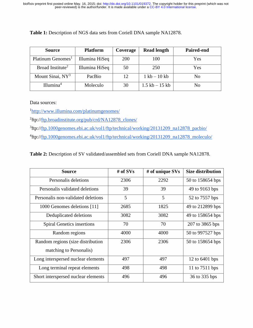
Table 1: Description of NGS data sets from Coriell DNA sample NA12878.

Source Platform Coverage Read length Paired-end

Platinum Genomes1 Illumina HiSeq 200 100 Yes

Broad Institute2 Illumina HiSeq 50 250 Yes

Mount Sinai, NY3 PacBio 12 1 kb – 10 kb No

Illumina4 Moleculo 30 1.5 kb – 15 kb No

Data sources:

1http://www.illumina.com/platinumgenomes/

2ftp://ftp.broadinstitute.org/pub/crd/NA12878_clones/

3ftp://ftp.1000genomes.ebi.ac.uk/vol1/ftp/technical/working/20131209_na12878_pacbio/

4ftp://ftp.1000genomes.ebi.ac.uk/vol1/ftp/technical/working/20131209_na12878_moleculo/

Table 2: Description of SV validated/assembled sets from Coriell DNA sample NA12878.

Source # of SVs # of unique SVs Size distribution

Personalis deletions 2306 2292 50 to 158654 bps

Personalis validated deletions 39 39 49 to 9163 bps

Personalis non-validated deletions 5 5 52 to 7557 bps

1000 Genomes deletions [11] 2685 1825 49 to 212899 bps

Deduplicated deletions 3082 3082 49 to 158654 bps

Spiral Genetics insertions 70 70 207 to 3865 bps

Random regions 4000 4000 50 to 997527 bps

Random regions (size distribution

matching to Personalis)

2306 2306 50 to 158654 bps

Long interspersed nuclear elements 497 497 12 to 6401 bps

Long terminal repeat elements 498 498 11 to 7511 bps

Short interspersed nuclear elements 496 496 36 to 335 bps


http://www.illumina.com/platinumgenomes/

http://ftp.broadinstitute.org/pub/crd/NA12878_clones/

http://ftp.1000genomes.ebi.ac.uk/vol1/ftp/technical/working/20131209_na12878_pacbio/

http://ftp.1000genomes.ebi.ac.uk/vol1/ftp/technical/working/20131209_na12878_moleculo/

http://dx.doi.org/10.1101/019372


Table 3: Analysis of 8 clusters from hierarchical cluster analysis, including the numbers of sites from each call set and a description of

the predominant types of sites in each cluster

Cluster 4000

Random

Personalis

Random

Random

LINEs

Random

LTRs

Random

SINEs

Personalis

deletions

1000

Genomes

deletions

Total Proportion

of

deletions

Description

1 0 0 0 0 0 371 284 655 1.000 Mostly large,

true

homozygous

deletions

2 0 0 0 0 2 432 237 671 0.997 Heterozygous

Alu deletions

3 1 1 1 0 0 705 402 1110 0.997 Homozygous

Alu deletions

4 2397 455 38 28 16 9 28 2971 0.012 Large, likely

non-SVs.

Generally in

easy-to-

sequence

regions

5 1073 1351 352 378 279 1 33 3467 0.010 Smaller, likely

non-SVs.


http://dx.doi.org/10.1101/019372


Generally in

easy-to-

sequence

regions

6 17 2 1 0 0 3 138 161 0.876 Likely true

large

homozygous

deletions with

inaccurate

breakpoints so

that the true

deletion is

larger than the

called region

7 14 16 2 2 4 624 811 1473 0.974 Mostly true

heterozygous

deletions in

easier-to-

sequence

regions

8 498 481 103 90 195 161 752 2280 0.400 Mix of non-

SVs and SVs


http://dx.doi.org/10.1101/019372


in more

difficult

regions with

coverage

between the

normal

coverage and

half the normal

coverage

Total 4000 2306 497 498 496 2306 2685 12788 0.390

Table 4: Number of sites from each candidate call set that have k=3 L1 Classification scores in each range, where the score is the

proportion p of random sites that are closer to the center than each candidate site. These numbers are after filtering sites for which the

flanking regions have low mapping quality or high coverage.

Filtered <0.68 0.68-0.9 0.9-0.97 0.97-0.99 0.99-0.997 0.997-0.999 >0.999

Random

Personalis 229 3025 501 177 65 3 0 0

Personalis

Gold 106 8 10 44 414 409 1302 13

Personalis

Validated

3 0 0 0 10 7 19 0


http://dx.doi.org/10.1101/019372


Personalis

Non-validated

0 1 0 0 3 0 1 0

1000

Genomes 382 56 103 257 714 388 780 5

Spiral Gen

Insertions 1 0 0 0 12 16 41 0

Deduplicated

Deletions 195 45 61 145 675 513 1434 14


http://dx.doi.org/10.1101/019372


Figure 1: Annotations are generated for each SV for five different regions in and around the SV:

Left flanking region (L), Left middle flanking region (LM), Middle regions based on SV

coordinates (M), Right middle flanking region (RM), and Right flanking region (R).

Figure 2: Depth of coverage distribution for Personalis deletion calls (PlatGen_M_Cov) and

random regions (PlatGen_Random_4000_M_Cov). See original data at

https://plot.ly/~justinzook/2.


https://plot.ly/~justinzook/2

http://dx.doi.org/10.1101/019372


Figure 3: Flowchart of analytical approach to classify candidate SVs into likely true or false

positives. The subset of 35 annotations was chosen for Illumina paired-end data (fewer for PacBio

and moleculo data) to reduce the number of annotations used in the model to those that we expected

to be most important for clustering calls into different categories. The one-class model uses only

the 4000 random sites for training, and it assumes that sites with annotations unlike most of these

random sites are more likely to be SVs.


http://dx.doi.org/10.1101/019372


(A)

(B) (C)

Figure 4: Hierarchical clustering results using L1 distance and Ward’s method shown as (A) a

dendrogram and (B-C) in multi-dimensional scaling plots. (A) The horizontal dotted red line

shows the cut-off at a cluster dissimilarity index of about 10000, which results in 8 clusters. The

clusters are number 1 to 8 from left to right, with 4 and 5 containing primarily non-SVs, 8

containing a mixture of SVs and non-SVs, and 1, 2, 3, 6, and 7 containing different types of

deletions (see Table 4). (B-C) Multidimensional scaling plots for visualizing the 8 clusters. We

use a 3 dimensional representation of the data space which associates 3 MDS coordinates to each

site, one for each dimension. (B) Plot of MDS-2 against MDS-1, which clearly separates Cluster

6 (mainly SVs with inaccurate breakpoints). (C) Plot of MDS-3 against MDS-1, in which the

different types of SVs are generally well-separated from each other and from non-SVs.


http://dx.doi.org/10.1101/019372


Figure 5: ROC curves for One-class classification using the L1 Distance, treating the 4000

Random regions as negatives and the Personalis or 1000 Genomes calls as positives. (A) ROC

curves for one-class models for each dataset separately and for all combined for the Personalis

validated deletion calls. (B) ROC curves for one-class models for each dataset separately and for

all combined for the 1000 Genomes validated deletion calls. (C) ROC curves for one-class model

requiring 1 or more, 2 or more, 3 or more, or all 4 technologies to have high classification scores

for the Personalis validated deletion calls. (D) ROC curves for one-class model requiring 1 or

more, 2 or more, 3 or more, or all 4 technologies to have high classification scores for the 1000

Genomes validated deletion calls. The 3 or more classification method is used to produce the final

high-confidence SVs in this work. The horizontal axis shows the false positive rate (from the

random set of regions matching the size distribution of the Personalis deletions) and the vertical

axis shows the corresponding true positive rate (assuming all the validated/assembled calls are

true). See original data at https://plot.ly/~desuchen0929/303, https://plot.ly/~desuchen0929/311,

https://plot.ly/~desuchen0929/319, and https://plot.ly/~desuchen0929/322.


https://plot.ly/~desuchen0929/303




http://dx.doi.org/10.1101/019372


Supplementary Information

1. Data transform for one- class SVM.

For a certain annotation, the “right-tail” case means outliers should have positive deviations, the

“left-tail” case means outliers should have negative deviations, and the “both-tail” case means that

outliers could have either positive or negative deviations. Reference deviations were then

calculated for different cases. For the left-tail and right-tail cases,

𝜎 = √∑𝑛𝑖=1 (𝑥𝑖 − 𝑥𝑒𝑥𝑡𝑟𝑒𝑚𝑒)2

𝑛

σ is the reference deviation, xi is annotation value of the ith site from the random regions. n is the

number of sites from the random regions (n = 4000). xextreme is either the minimum of xi for the

right-tail case, or the maximum of xi for left-tail case. For any observation x of the same

annotation for any SV, the transform y is

𝑦 = 2/(1 + 𝑐𝑜𝑠ℎ(|𝑥 − 𝑥𝑒𝑥𝑡𝑟𝑒𝑚𝑒|/𝜎))

For both-tail case, we define two reference deviations σright and σleft for either positive or negative

deviations from the median xmed of xi,

𝜎𝑟𝑖𝑔ℎ𝑡 = √∑𝑥𝑖>𝑥𝑚𝑒𝑑

(𝑥𝑖 − 𝑥𝑚𝑒𝑑)2

∑𝑥𝑖>𝑥𝑚𝑒𝑑1

, 𝜎𝑙𝑒𝑓𝑡 = √∑𝑥𝑖<𝑥𝑚𝑒𝑑

(𝑥𝑖 − 𝑥𝑚𝑒𝑑)2

∑𝑥𝑖<𝑥𝑚𝑒𝑑1

The transform y is

𝑦 = 2/(1 + 𝑐𝑜𝑠ℎ(|𝑥 − 𝑥𝑚𝑒𝑑|/𝜎𝑟𝑖𝑔ℎ𝑡)), if x > xmed

𝑦 = 2/(1 + 𝑐𝑜𝑠ℎ(|𝑥 − 𝑥𝑚𝑒𝑑|/𝜎𝑙𝑒𝑓𝑡)), if x < xmed

y = 0, if x = xmed

Therefore outliers indicating potential SVs approach 0 in this transform, which is required by the

application of one-class SVM. In the transformed metric space, linear classifiers were trained by

the one-class SVM (implemented with package e1071 in the Comprehensive R Archive Network)

with SVs from the random regions as the training set. The proportion of SVs in the training set

identified as outliers (false positive rate) 1-p was approximately controlled by a factor ν in the

training algorithm defined by the authors. In short, ν ∈ (0,1) defines the ratio of penalty induced

by margin size (e.g. distance from origin point to the class boundary with linear kernel) and penalty

induced by number of outliers in the training set in the total penalty function for soft margin case.


http://dx.doi.org/10.1101/019372


Higher ν allows more training data points to be on the outliers side to maximize the margin.

Classifiers at different ν’s were then applied to predict other SV data sets.

Supplementary figure 1: ROC curves for One-class classification using SVM, treating the 4000

Random regions as negatives and the Personalis or 1000 Genomes calls as positives. (A) ROC

curves for one-class models for each dataset separately and for all combined for the Personalis

validated deletion calls. (B) ROC curves for one-class models for each dataset separately and for

all combined for the 1000 Genomes validated deletion calls. (C) ROC curves for one-class model

requiring 1 or more, 2 or more, 3 or more, or all 4 technologies to have high classification scores

for the Personalis validated deletion calls. (D) ROC curves for one-class model requiring 1 or

more, 2 or more, 3 or more, or all 4 technologies to have high classification scores for the 1000

Genomes validated deletion calls. See original data at https://plot.ly/~desuchen0929/325,

https://plot.ly/~desuchen0929/328, https://plot.ly/~desuchen0929/331, and

https://plot.ly/~desuchen0929/337.






http://dx.doi.org/10.1101/019372


Supplementary figure 2: ROC curves for One-class classification using SVM and L1 “3 or more”

strategy, treating the 4000 random regions as training negatives, treating (A) the Personalis

deletion calls and (B) the 1000 Genomes deletion calls as testing positives and treating the 2306

random regions as testing negatives. See original data at https://plot.ly/~desuchen0929/341, and





http://dx.doi.org/10.1101/019372


Supplementary figure 3: ROC curves for One-class classification using SVM, treating the 4000

random regions as negatives and the Spiral Genetics insertions calls as positives. (A) ROC curves

for one-class models for each dataset separately and for all combined. (B) ROC curves for one-

class model requiring 1 or more, 2 or more, 3 or more, or all 4 technologies to have high

classification scores. See original data at https://plot.ly/~desuchen0929/391, and





http://dx.doi.org/10.1101/019372


Supplementary figure 4: ROC curves for One-class classification using the L1 Distance, treating

the 4000 random regions as negatives and the Spiral Genetics insertions calls as positives. (A)

ROC curves for one-class models for each dataset separately and for all combined. (B) ROC

curves for one-class model requiring 1 or more, 2 or more, 3 or more, or all 4 technologies to have

high classification scores. See original data at https://plot.ly/~desuchen0929/386, and





http://dx.doi.org/10.1101/019372


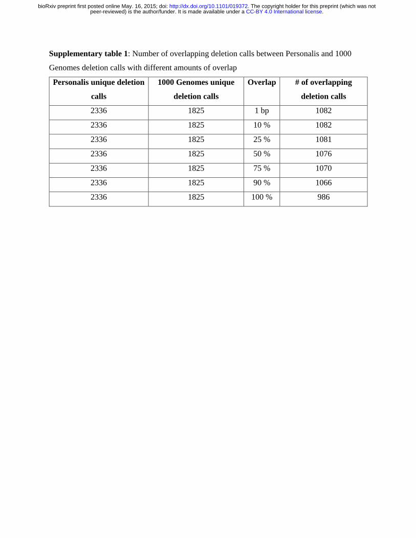
Supplementary table 1: Number of overlapping deletion calls between Personalis and 1000

Genomes deletion calls with different amounts of overlap

Personalis unique deletion

calls

1000 Genomes unique

deletion calls

Overlap # of overlapping

deletion calls

2336 1825 1 bp 1082

2336 1825 10 % 1082

2336 1825 25 % 1081

2336 1825 50 % 1076

2336 1825 75 % 1070

2336 1825 90 % 1066

2336 1825 100 % 986


http://dx.doi.org/10.1101/019372


Supplementary table 2: Output format of svclassify

svclassify generates 85 to 180 annotations for each SV from each aligned sequence data, depending

on sequencing technology.

SV_size: The SV_size gives the size of a structural variant (SV).

SV_Cat: The SV_Cat gives the size distribution of a SV as a categorical value (i.e. SV size of <

100 = 0, SV size of >=100 to <1000 = 1, SV size of >=1000 to <10000 = 2, SV size of >=10000

= 3).

Each SV is characterized in five groups (please refer to Figure 1):

(1) Left flanking region (L)

(2) Left middle flanking region (LM)

(3) Middle regions based on SV coordinates (M)

(4) Right middle flanking region (RM)

(5) Right flanking region (R)

Cov: The Cov gives the mean of depth of coverage.

Cov_sd: The Cov_sd gives the standard deviation of depth of coverage.

Cov_pro: The Cov_pro gives the proportion of the SV with depth of coverage less than 5X.

Insert: The Insert gives the mean of insert size of paired reads (samtools flags of -f2).

Insert_sd: The Insert_sd gives the standard deviation of insert size of paired reads.

Insert_10_percentile: The Insert_10_percentile gives the 10th percentile of insert size distribution

of paired reads.

Insert_90_percentile: The Insert_90_percentile gives the 90th percentile of insert size distribution

of paired reads.

Dis_unmap: The Dis_unmap gives numbers of the unmapped mate (samtools flags of -f9 -F

1792).

Dis_map: The Dis_map gives numbers of the mapped mate in reverse orientation (samtools flags

of -f1 -F 1802).

Dis_all: The Dis_all gives numbers of the total paired reads (samtools flag of -f2).


http://dx.doi.org/10.1101/019372


Dis_unmap_ratio: The Dis_unmap_ratio gives the ratio of numbers of the unmapped mate to

numbers of total paired reads.

Dis_map_ratio: The Dis_map_ratio gives the ratio of numbers of the mapped mate in reverse

orientation to numbers of total paired reads.

Mapping_q: The Mapping_q gives the mean of mapping quality of the reads.

Mapping_q_sd: The Mapping_q_sd gives the standard deviation of mapping quality of the reads.

Mapping_pro: The Mapping_pro gives the proportion of reads with mapping quality of zero.

Mapping_10_percentile: The Mapping_10_percentile gives the 10th percentile of mapping

quality distribution of the reads.

Mapping_90_percentile: The Mapping_90_percentile gives the 90th percentile of mapping

quality distribution of the reads.

Soft: The Soft gives the mean of soft clipped bases of the reads.

Soft_sd: The Soft_sd gives the standard deviation of soft clipped bases of the reads.

Soft_pro: The Soft_pro gives the proportion of the reads with soft clipped bases greater than 5.

Soft_10_percentile: The Soft_10_percentile gives the 10th percentile of soft clipped bases of the

reads distribution.

Soft_90_percentile: The Soft_90_percentile gives the 90th percentile of soft clipped bases of the

reads distribution.

Del: The Del gives the mean of deleted bases of the reads.

Del_sd: The Del_sd gives the standard deviation of deleted bases of the reads.

Del_10_percentile: The Del_10_percentile gives the 10th percentile of deleted bases of the reads

distribution.

Del_90_percentile: The Del_90_percentile gives the 90th percentile of deleted bases of the reads

distribution.

Ins: The Ins gives the mean of inserted bases of the reads.

Ins_sd: The Ins_sd gives the standard deviation of inserted bases of the reads.

Ins_10_percentile: The Ins_10_percentile gives the 10th percentile of inserted bases of the reads

distribution.

Ins_90_percentile: The Ins_90_percentile gives the 90th percentile of inserted bases of the reads

distribution.


http://dx.doi.org/10.1101/019372


Diff: The Diff gives the mean of differences between numbers of inserted and numbers of deleted

bases of the reads.

Diff_sd: The Diff_sd gives the standard deviation of differences between numbers of inserted

and numbers of deleted bases of the reads.

Diff_10_percentile: The Diff_10_percentile gives the 10th percentile of differences between

numbers of inserted and numbers of deleted bases distribution of the reads.

Diff_90_percentile: The Diff_90_percentile gives the 90th percentile of differences between

numbers of inserted and numbers of deleted bases distribution of the reads.

M_Cov_Cat: The M_Cov_Cat gives the coverage distribution of a SV as a categorical based on

user defined input coverage_cutoff value.

M_Homvar: The M_Homvar gives the number of homozygous SNP genotype calls inside the

SV.

M_Homvar_SV: The M_Homvar_SV gives the ratio of number of homozygous SNP genotype

calls inside the SV to the size of SV.

M_Hetvar: The M_Hetvar gives the number of heterozygous SNP genotype calls inside the SV.

M_Hetvar_SV: The M_Hetvar_SV gives the ratio of number of heterozygous SNP genotype calls

inside the SV to the size of SV.

M_GCcontent: The M_GCcontent gives the percentage of GC content to the size of SV.

M_Sine_Line_Ltr_SV: The M_Sine_Line_Ltr_SV gives the percentage of short interspersed

nuclear elements (SINE), long interspersed nuclear elements (LINE) and long terminal repeat

elements (LTR) identified by RepeatMasker to the size of SV.

M_Simple_Low_Satellite_SV: The M_Simple_Low_Satellite_SV gives the percentage of simple,

low complexity and satellite repeats identified by RepeatMasker to the size of SV.

Supplementary table 3: Selected characteristics for hierarchical clustering and One-class

models

For Illumina and moleculo datasets:

M_Cov, M_Cov_sd, M_Insert_sd, M_Dis_unmap_ratio, M_Dis_map_ratio, M_Soft_pro,

M_Homvar_SV, M_Hetvar_SV


http://dx.doi.org/10.1101/019372


L_Insert_90_percentile, L_Dis_unmap_ratio, L_Dis_map_ratio, L_Soft_90_percentile, L_Cov,

L_Insert_sd, L_Soft_pro

R_Insert_90_percentile, R_Dis_unmap_ratio, R_Dis_map_ratio, R_Soft_90_percentile, R_Cov

LM_Insert_90_percentile, LM_Dis_unmap_ratio, LM_Dis_map_ratio, LM_Soft_90_percentile,

LM_Cov

RM_Insert_90_percentile, RM_Dis_unmap_ratio, RM_Dis_map_ratio, RM_Soft_90_percentile,

RM_Cov

R_Insert_90_percentile, R_Dis_unmap_ratio, R_Dis_map_ratio, R_Soft_90_percentile, R_Cov

For PacBio datasets:

L_Diff, R_Diff, M_Cov, M_Del, M_Ins, M_Diff, M_Diff_sd

For hierarchical clustering only:

SV_size, M_Mapping_q, M_Sine_Line_Ltr_SV, M_GC_Content, and

M_Simple_Low_Satellite_SV

- Note also that all of these except M_Mapping_q are the same for all of the datasets so only

need to be included once for the joint dataset unsupervised analysis.

Supplementary table 8: Elements of concordance/discordance matrix of predictions on Personalis

validated/assembled set by the one-class L1 classifier and one-class SVM with annotations of all

technologies combined.

p 0.99 0.95 0.9 0.68

SVM(+), L1(+) 1665 2291 2302 2306

SVM(+), L1(-) 458 4 1 0

SVM(-), L1(+) 10 5 0 0

SVM(-), L1(-) 173 6 3 0


http://dx.doi.org/10.1101/019372


Elements of concordance/ discordance matrix of predictions on Personalis validated/assembled set

with ensemble classifiers (k=3) of one-class L1 classifier and one-class SVM.

p 0.99 0.95 0.9 0.68

SVM(+), L1(+) 1711 2232 2275 2296

SVM(+), L1(-) 341 12 4 3

SVM(-), L1(+) 45 35 11 1

SVM(-), L1(-) 209 27 16 6

Elements of concordance/Discordance matrix of predictions on 1000 Genomes set by the one-class

L1 classifier and one-class SVM with annotations of all technologies combined.

P 0.99 0.95 0.9 0.68

SVM(+), L1(+) 1188 2373 2567 2654

SVM(+), L1(-) 598 100 51 7

SVM(-), L1(+) 100 43 7 8

SVM(-), L1(-) 799 169 60 16

Elements of concordance/ discordance matrix of predictions on 1000 Genomes set with ensemble

classifiers (k=3) of one-class L1 classifier and one-class SVM.

p 0.99 0.95 0.9 0.68

SVM(+), L1(+) 1189 2161 2405 2598

SVM(+), L1(-) 463 93 69 41

SVM(-), L1(+) 176 150 75 16

SVM(-), L1(-) 857 281 136 30


http://dx.doi.org/10.1101/019372



http://dx.doi.org/10.1101/019372


svclassify: a method to establish benchmark structural ... · biorxiv preprint first posted online...

Documents