sustainable engineering internship - shoals marine … · sustainable engineering internship 26...
TRANSCRIPT

Sustainable
Engineering
Internship 26 July 2015
Chelsea Kimball, Dylan Masi, Susan McGrattan, Marisa Zellmer

S E I 2 0 1 5 F i n a l R e p o r t P a g e | 2
Table of Contents
List of Figures .................................................................................................................................7
List of Tables ..................................................................................................................................8
List of Equations ............................................................................................................................8
Executive Summary .......................................................................................................................9
Introduction ..................................................................................................................................9
Project 1 – LED Lighting Survey .................................................................................................9
Project 2 – ECB Performance / Dashboard .................................................................................9
Project 3 – Saltwater Pump Efficiency .....................................................................................10
Project 4 – Electrical Transformer Study ...................................................................................10
Project 5 – Electrical Load Profiles ............................................................................................10
Project 6 – Rainwater Collection for Celia Thaxter’s Garden ...................................................11
Project 7 – Freshwater Well Siting ...........................................................................................11
Electrical Energy Conservation ..................................................................................................12
1 – LED Lighting Study ...............................................................................................................12
1.1 Background ..........................................................................................................................12
1.2 Purpose .................................................................................................................................12
1.3 Scope ....................................................................................................................................12
1.4 Methods ................................................................................................................................12
1.4.1 Survey ............................................................................................................................12
1.4.2 Audit ..............................................................................................................................12
1.5 Results and Analysis ............................................................................................................13
1.5.1 Survey Results ...............................................................................................................13
1.5.2 Audit Results .................................................................................................................15
1.5.3 Cost Analyses ................................................................................................................16
1.6 Conclusions and Recommendations .....................................................................................17
1.6.1 Solar Tube Option .........................................................................................................17
1.6.2 Retrofit Recommendations ............................................................................................17
1.6.3 Outdoor Lighting Recommendations ............................................................................17
1.7 References ............................................................................................................................18
2 – ECB Performance / Dashboard ............................................................................................19
2.1 Background .........................................................................................................................19
2.2 Purpose .................................................................................................................................19

S E I 2 0 1 5 F i n a l R e p o r t P a g e | 3
2.3 Scope ....................................................................................................................................20
2.4 Methods ................................................................................................................................20
2.4.1 Battery Monitor Reliability ..........................................................................................20
2.4.2 Solar Panel Performance ..............................................................................................20
2.4.3 Dashboard ......................................................................................................................21
2.5 Results and Analysis ............................................................................................................21
2.5.1 Battery Monitor Reliability ..........................................................................................21
2.5.2 Solar Panel Performance ..............................................................................................24
2.5.2.1 Comparing Generator Run Times ..........................................................................25
2.5.2.2 Percent Power .......................................................................................................26
2.5.2.3 Diesel Fuel Consumption .......................................................................................27
2.5.3 Dashboard .....................................................................................................................28
2.6 Conclusions and Recommendations .....................................................................................28
2.6.1 Battery Monitor Reliability ...........................................................................................28
2.6.2 Solar Panel Performance ...............................................................................................29
2.6.3 Dashboard ......................................................................................................................29
2.7 References ............................................................................................................................29
3 – Saltwater Pump Efficiency ....................................................................................................30
3.1 Background .........................................................................................................................30
3.2 Purpose .................................................................................................................................30
3.3 Scope ....................................................................................................................................31
3.4 Methods ................................................................................................................................31
3.4.1 Electrical Energy Draw ................................................................................................31
3.4.2 Maximum Flow Rate .....................................................................................................31
3.4.3 Elevation of Pump Above Low Tide ............................................................................31
3.5 Results and Analysis ............................................................................................................32
3.5.1 Electrical Draw of Saltwater Pump ..............................................................................32
3.5.2 Maximum Flow Rate of Saltwater Pump .....................................................................33
3.5.3 Net Positive Suction Head Calculations ........................................................................33
3.5.4 System Curve Calculations............................................................................................35
3.5.5 System and Pump Curve Analyses ................................................................................36
3.6 Conclusions and Recommendations .....................................................................................38
3.6.1 Replacement Options and Cost Analysis ......................................................................38

S E I 2 0 1 5 F i n a l R e p o r t P a g e | 4
3.6.2 Submersible Replacement Pump Analysis ....................................................................39
3.6.3 Centrifugal Replacement Pump Analysis ......................................................................40
3.6.4 Net Positive Suction Head Recommendations ..............................................................40
3.6.5 Variable Frequency Drive Recommendation ...............................................................41
3.7 References ............................................................................................................................42
4 – Transformer Efficiency Study ..............................................................................................43
4.1 Background .........................................................................................................................43
4.2 Purpose .................................................................................................................................43
4.3 Scope ....................................................................................................................................43
4.4 Methods ................................................................................................................................44
4.4.1 Preliminary Research ....................................................................................................44
4.4.2 Eagle 440 Meter ............................................................................................................44
4.4.3 Line Losses ...................................................................................................................44
4.4.4 Transformer Efficiencies ..............................................................................................44
4.5 Results and Analysis ............................................................................................................45
4.6 Conclusions and Recommendations .....................................................................................47
4.7 References ............................................................................................................................47
5 – Electrical Load Profiles .........................................................................................................48
5.1 Background .........................................................................................................................48
5.2 Purpose .................................................................................................................................48
5.3 Scope ....................................................................................................................................48
5.4 Methods ................................................................................................................................48
5.4.1 Eagle 440 Transformer Readings By Building .............................................................48
5.4.2 Electrical Appliance By Building ..................................................................................48
5.4.3 Island Energy and Population Comparison ..................................................................49
5.5 Results and Analysis ............................................................................................................49
5.5.1 Eagle 440 Results By Building .....................................................................................49
5.5.2 Electrical Appliance By Building .................................................................................50
5.5.3 Island Energy Per Person ..............................................................................................52
5.6 Conclusions and Recommendations .....................................................................................53
5.6.1 Conservation Strategies By Building ...........................................................................53
5.6.2 Water Conservation is Also Energy Conservation ........................................................53
5.6.3 Moving Loads to Daytime .............................................................................................54
5.6.4 Energy Use Per Person .................................................................................................54

S E I 2 0 1 5 F i n a l R e p o r t P a g e | 5
5.7 References ............................................................................................................................54
Water Resources ..........................................................................................................................55
6 – Rainwater Collection for Celia Thaxter’s Garden .............................................................55
6.1 Background .........................................................................................................................55
6.2 Purpose .................................................................................................................................55
6.3 Scope ....................................................................................................................................55
6.4 Methods ................................................................................................................................55
6.4.1 Filtration System ..........................................................................................................55
6.4.2 Watering Method ..........................................................................................................55
6.4.3 Pump Selection .............................................................................................................56
6.5 Results and Analysis ............................................................................................................56
6.5.1 Filtration Methods .........................................................................................................56
6.5.1.1 Filtration Method 1: Gutter Filters .........................................................................56
6.5.1.2 Filtration Method 2: First Flush .............................................................................57
6.5.2 Watering Methods .........................................................................................................58
6.5.2.1 Watering Method 1: Sprinklers ..............................................................................58
6.5.2.2 Watering Method 2: Drip Irrigation ......................................................................59
6.5.3 Tank Size Evaluation ....................................................................................................60
6.5.4 Pump Calculations and Options ...................................................................................62
6.6 Conclusions and Recommendations .....................................................................................64
6.6.1 Filtration and Watering Method Recommendations ....................................................64
6.6.1 Pump Recommendation.................................................................................................65
6.7 References ............................................................................................................................66
7 – Freshwater Well Siting ..........................................................................................................67
7.1 Background .........................................................................................................................67
7.2 Purpose .................................................................................................................................67
7.3 Scope ....................................................................................................................................67
7.4 Methods ................................................................................................................................67
7.4.1 Calculating Leakage .....................................................................................................67
7.4.2 Evaluating New Well Site ............................................................................................67
7.5 Results and Analysis ............................................................................................................67
7.5.1 Calculating Leakage .....................................................................................................67
7.5.2 Evaluating New Well Site ............................................................................................72
7.6 Conclusions and Recommendations .....................................................................................72

S E I 2 0 1 5 F i n a l R e p o r t P a g e | 6
7.7 References ............................................................................................................................73
8 – Future Project Recommendations ........................................................................................74
Correcting and Updating GIS Map
Well Site to Capture Leakage from Current Well
Well Site Next to Crystal Lake to Capture Spring Water
Bird Deterrents to Increase Solar Panel Efficiency
Look at Electrical Load Compared to the Number and Type of People on Island
Acknowledgements ......................................................................................................................75
Appendix .......................................................................................................................................76

S E I 2 0 1 5 F i n a l R e p o r t P a g e | 7
List of Figures
Figure 1: Daytime Lighting Quality Survey Responses................................................................13
Figure 2: Nighttime and Rainy Day Lighting Quality Survey Responses.....................................14
Figure 3: Most Frequented Buildings at Night - Based on Survey Responses..............................14
Figure 4: Nighttime Pathway Safety Survey Responses................................................................15
Figure 5: Outdoor Additional Pathway Lights...............................................................................18
Figure 6: Battery Bank 6 Voltage..................................................................................................21
Figure 7: Battery Bank 6 Current...................................................................................................22
Figure 8: Battery Bank 2 Voltage..................................................................................................22
Figure 9: Battery Bank 2 Current...................................................................................................23
Figure 10: Voltage Average Differences.......................................................................................24
Figure 11: Current Average Differences........................................................................................24
Figure 12: Generator Run Times 2014 and 2015...........................................................................25
Figure 13: 2014 Island Power Breakdown.....................................................................................27
Figure 14: 2015 Island Power Breakdown.....................................................................................27
Figure 15: GIS Graphic of Current Saltwater System...................................................................30
Figure 16: Recorded Energy Use of Salt Water Pump from Manual Shut Off.............................32
Figure 17: Recorded Energy Use of Salt Water Pump from Eagle 440 Meter..............................33
Figure 18: Current Pump - System Curve......................................................................................36
Figure 19: Current Pump - Pump Curve........................................................................................37
Figure 20: Operating Point of Current System..............................................................................38
Figure 21: Analysis of Submersible Pump Option with System Curve.........................................39
Figure 22: Analysis of Centrifugal Pump Option with System Curve..........................................40
Figure 23: Energy Conservation Building Apparent Power..........................................................46
Figure 24: Electrical Load of Kiggins Commons Over 42 Hours.................................................49
Figure 25: Average Daily Energy Use...........................................................................................50
Figure 26: Percent of Total Power Used By Each Building..........................................................52
Figure 27: Island Population by Energy Used Each Day..............................................................53
Figure 28: Filter A (left) and Filter B (right).................................................................................56
Figure 29: Effectiveness of Filter Designs.....................................................................................57
Figure 30: First Flush CAD Drawing............................................................................................57
Figure 31: First Flush Diagram......................................................................................................58
Figure 32: Current Sprinkler Locations.........................................................................................58
Figure 33: Drip Irrigation Hose Layout.........................................................................................59
Figure 34: Netafim Product Specifications....................................................................................60
Figure 35: Fullness of Rainwater Tank With Gutter Filters..........................................................61
Figure 36: Fullness of Rainwater With First Flush........................................................................61
Figure 37: Pump Curve of Recommended Pump..........................................................................65
Figure 38: Winter 2014-2015 Well Data.......................................................................................68
Figure 39: Summer 2015 Well Data..............................................................................................68

S E I 2 0 1 5 F i n a l R e p o r t P a g e | 8
Figure 40: Rainfall and Well Height..............................................................................................69
Figure 41: Area with Respect to Height........................................................................................70
Figure 42: Calculating Leakage Between Rainfall Events............................................................71
List of Tables
Table 1: Illuminance Comparison Between LED and Fluorescent...............................................16
Table 2: Indoor Lighting Cost Analysis.........................................................................................16
Table 3: Outdoor Lighting Cost Analysis......................................................................................17
Table 4: Voltage Average Difference (V).....................................................................................23
Table 5: Current Average Difference (A)......................................................................................23
Table 6: Average Generator Hours Run per Night Each Month...................................................26
Table 7: Percent Power from Generator........................................................................................26
Table 8: Diesel Fuel Consumption................................................................................................28
Table 9: Elevation Difference Between Low Tide and Pump.......................................................34
Table 10: Cost Analysis of Saltwater Options...............................................................................38
Table 11: Net Positive Suction Head.............................................................................................41
Table 12: Losses Based on Transformer Impedance.....................................................................45
Table 13: Losses Based on Percent Load......................................................................................45
Table 14: Transformer Efficiencies...............................................................................................46
Table 15: Electrical Appliance Audit for Bartels..........................................................................51
Table 16: Calculating Head for Sprinkler and Drip Irrigation Systems........................................63
Table 17: Pump Options................................................................................................................63
Table 18: Comparison of Filtration Methods.................................................................................64
Table 19: Comparison of Watering Methods.................................................................................64
Table 20: Effect of Rainfall on Watershed....................................................................................70
Table 21: Well Leakage.................................................................................................................72
Table 22: New Well Site Testing...................................................................................................72
List of Equations
Equation 1: Net Positive Suction Head..........................................................................................34
Equation 2: Net Positive Suction Head Apparent and Required...................................................35
Equation 3: System Curve.............................................................................................................35
Equation 4: Transformer Efficiencies............................................................................................46
Equation 5: Head Pump Calculation..............................................................................................62
Equation 6: Area of Formation......................................................................................................69
Equation 7: Leakage As A Function of Well Depth......................................................................71

S E I 2 0 1 5 F i n a l R e p o r t P a g e | 9
Executive Summary
Introduction
Since 2006, Shoals Marine Laboratory (SML) has sponsored the Sustainable Engineering
Internship (SEI). Over the past ten years, interns have completed projects designed to increase the
sustainability on Appledore Island. This year the interns have seven projects. Five of these focus
on electrical energy conservation and two focus on water resources. The seven projects this year
are titled LED Lighting Study, Performance of the Battery Banks in the Energy Conservation
Building/Dashboard, Pumping Salt Water More Efficiently, Electrical Transformer Study,
Electrical Load Profiles, Rainwater Collection for Celia Thaxter’s Garden, and Siting a New Well
on Appledore. This document includes background, purpose, scope, methods, results, analyses,
conclusions, and recommendations.
Project 1 - LED Lighting Study
The lighting needs and current system for both indoor and outdoor lights were studied by
developing a survey for island residents and executing a campus wide audit. The results of the
survey yielded information that the current lighting system provided adequate lighting. The survey
also revealed which pathways were most frequently used at night and that half the island
population believes the pathways to be unsafe for walking at night. The audit aided in determining
that the current lights could be replaced with LED equivalents in an equal ratio by testing light
levels of important working surfaces. The audit also allowed for the creation of the cost analysis
for an LED retrofit of the entire campus. The cost analysis revealed that an island wide retrofit for
both indoor and outdoor lighting would significantly decrease energy usage and cost.
Recommendations were made for the placement of additional pathway lighting to increase the
safety of pathways for walking at night.
Project 2 - ECB Performance / Dashboard
The Energy Conservation Building was built in 2013, and a 300 kWh battery bank system
was installed in 2014. The final installation of solar panels was finished in the beginning of July
in 2015 and the interns determined that the solar panels are working efficiently because they found
a decrease in the generator hour run time, percent of total island power coming from the generator,
and gallons of diesel fuel used from 2014 to 2015. The interns also measured the reliability of the
battery monitor that is permanently installed on Battery Bank 6, and they determined if the
automatic generator system (AGS) should be making decisions based off of current or voltage. A
fluke meter was set up on Battery Bank 6 to measure current and voltage. Since similar
measurements were recorded, it was concluded that the fluke meter gave accurate measurements.
The fluke meter was then set up on each of the other nine battery banks, while the battery monitor
remained on Battery Bank 6, to measure the current and voltage in each of the other battery banks
compared to Battery Bank 6. The interns found that Battery Bank 2 and possibly Battery Bank 9
may not be charging the same as the other batteries, and recommend that this be further

S E I 2 0 1 5 F i n a l R e p o r t P a g e | 10
investigated by SML staff or future interns. Finally, the interns contacted Cornell Dashboard
representatives to continue the progress of setting up a Dashboard page for SML. The interns
contacted the Dashboard representatives and told them what items to display on the SML
Dashboard page. SML now needs to continue contact with the Cornell representatives so the SML
page will go online. SML should also contact UNH IT to see if they can also display data on the
UNH Dashboard. SML should also contact UNH IT to see if an SML page can also be added to
the UNH Dashboard.
Project 3 - Saltwater Pump Efficiency
In an attempt to reduce the energy which the saltwater pump uses, a three part study was
conducted. The first part included an analysis of how much power the saltwater pump required,
and the draw was found to be 3.5kW. This value was found by using a power meter test and manual
shut off tests. This verified that resizing the pump would significantly reduce the total island load.
The system curve was then calculated and plotted with the current pump curve and two viable
replacement options. However, the Net Positive Suction Head Available for the system must first
be reliably calculated before deciding to purchase a pump. The centrifugal pump replacement was
recommended because in the cost analysis it reduced the energy and cost significantly. The
centrifugal pump also did not require any significant changes in infrastructure which would allow
for simple maintenance. The centrifugal pump replacement was from Grundfos and its model
number is 97524349.
Project 4 - Electrical Transformer Study
The island has a transformer network that provides power in the necessary voltage for each
building. The interns calculated what the electrical losses are for the current network and what
they would be if some of the transformers were removed. The only transformers that could be
removed are the ones in Bartels, Laighton, and K-House. In each of these buildings, there would
be more electrical losses if the transformers were removed than if they are kept there, so the interns
do not recommend any of these be removed. Also, based on the Eagle 440 meter measurements of
what the average loads of the buildings were, the interns found the efficiency of each transformer.
The interns found that Bartels, Laighton, K-House, and the Utility Building have low transformer
efficiencies (lower than 90%). In addition, the Eagle 440 meter measured what the maximum load
of each building was, which should be used to size the transformers in each building. A cost
analysis should be performed to determine if SML should replace these four transformers with
transformers that are sized better to fit the maximum load of each building.
Project 5 - Electrical Load Profiles
The Eagle 440 data collected in the transformer study was used for the electrical load
profiles. The buildings and appliances that the power meter collected data for were displayed in a
graph which allowed for comparison and provided insight in where conservation is most needed.
The two largest electrical loads were from Kiggins Commons and the saltwater pump. The

S E I 2 0 1 5 F i n a l R e p o r t P a g e | 11
appliance audit for the island also allowed for comparison between buildings; the wattage for each
building and estimated energy load were both compared. Kiggins Commons, Bartels, and the
reverse osmosis machine were the largest loads on the island. The energy used for each person was
recorded for twelve days, and the results yielded that 5.7 kWh were used on average each day per
person. Future recommendations for the project included implementing conservation strategies,
metering buildings, and conducting a more comprehensive energy per person study.
Project 6 - Rainwater Collection for Celia Thaxter’s Garden
Celia Thaxter’s Garden is a historical part of Appledore Island. SML staff maintains and
gives tours of this garden. It is currently watered with potable water through a sprinkler system
that is set to turn on every day for 20 minutes. Early in the 2015 season, SML staff installed two
800-gallon tanks to catch rainwater off the Utility Building roof for watering the garden. The
interns experimented with small filtration devices and sized a first flush method to keep large
particles out of the collection tanks. A drip irrigation system was also investigated as a possible
replacement for the sprinklers. The interns recommend that SML switches to watering the garden
with a drip irrigation system and to use the first flush method to filter the water. A Grainger Dayton
pump was chosen to distribute the water to the garden at the required total head and flow rate.
Project 7 - Freshwater Well Siting
A 20-foot dug well currently supplies freshwater to the island. During dry seasons, a
reverse osmosis machine must be used to meet the freshwater demand of the island. This machine
is costly to use and is energy intensive. Meters were placed in the well over the autumn of 2014
through the summer of 2015. From this data, the interns tried to determine how much water was
leaking out of the well. This was done by determining the area and leakage of the well at different
depths. For both calculations, there were not enough data points to get an accurate representation
of the system. The meter was redeployed to provide SML with more data points. There should be
another study done to further investigate the leakage of the well. If there is a large amount of water
leaking out, then SML should consider putting a new well into a spot within the same watershed
that will capture this leakage. If this leakage is not significant, then SML should consider a new
well site. One potential new well site was studied by the interns. This new well site is located near
North Pond and is in a different watershed than the current well. The interns did measurements to
determine where the bedrock level was and how deep the saturated thickness level was. It was
found that the bedrock was no more than 2.5 feet below the surface and the greatest saturated
thickness was 13.5 inches, so this may not be deep enough to put in a horizontal well. Further
studies should be done, possibly with a ground penetrating radar, to determine if this new well site
would be able to provide enough water to supplement the current well.

S E I 2 0 1 5 F i n a l R e p o r t P a g e | 12
Electrical Energy Conservation
Project 1 - LED Lighting Study
1.1 Background
The current lighting systems at SML can be upgraded to increase energy efficiency and to
fit the needs of island residents more closely. By determining current lighting system conditions
and needs, a retrofit of the lighting system can be implemented with Light Emitting Diode (LED)
technology. The LED technology is expected to reduce electrical load on the system because it has
low wattage and long bulb life expectancy.
There is also a concern over a lack of outdoor lighting along walking paths, which may be
a safety concern for island residents after dark. By determining the most frequently trafficked paths
at night, a useful design of outdoor LED lighting can be recommended.
1.2 Purpose
In order to make well informed decisions about an LED retrofit, SML requested a study of
the current system and energy efficient options. The new LED lights should provide sufficient
lighting for the needs of each location while saving energy and not having an unnecessarily high
capital cost. This will further conserve energy at SML.
1.3 Scope
This project evaluates the island’s lighting needs, which includes both indoor and outdoor
systems. The lighting needs were also considered during different times of day and weather
conditions. This information was obtained through surveys of island inhabitants and is organized
and displayed in bar charts and pie charts. A cost analysis of retrofitting the island with LED lights
to fulfill lighting needs is included.
1.4 Methods
1.4.1 Survey
A survey of island residents was conducted from July 3rd to July 6th which assisted in
determining the current quality of lighting in each building on the SML campus. The survey
included criteria: “Good,” “Too Bright,” and “Too Dim,” for several rooms on the island.
Residents were asked whether outdoor night lighting was adequate for safe walking. Thirty island
residents responded, which was approximately 40% of the island population at the time of the
survey. An even mix of staff, faculty, and students responded to the survey.
1.4.2 Audit
Each building and room type (i.e. classroom, office, dorm) throughout the SML campus
was analyzed for number of bulbs, type of bulb, light levels on important surfaces with the lights
on and off during sunny and rainy days, and at night with the lights on. The amount of window

S E I 2 0 1 5 F i n a l R e p o r t P a g e | 13
area was estimated in each room to make recommendations about using the current lighting during
the day. The outdoor lights on buildings and pathways were included in the analysis of number
and type of bulbs.
1.5 Results & Analysis
1.5.1 Survey Results
In the survey island residents were asked to rate the quality of light in various rooms during
different times of day and weather conditions. The survey also included a short-answer question
regarding which pathways residents traveled at night and their opinion on the safety of island
pathways.
The majority of residents for each room replied that there was adequate lighting available.
There were more “Too Bright” responses during the day and more “Too Dim” responses at night,
which is to be expected because of sunlight levels. However, the number of “Good” responses was
greater than the “Too Bright” and “Too Dim” responses combined for all buildings. As a result, it
was determined that changes in light level were most likely unnecessary.
Figure 43: Daytime Lighting Quality Survey Responses

S E I 2 0 1 5 F i n a l R e p o r t P a g e | 14
Figure 44: Nighttime and Rainy Day Lighting Quality Survey Responses
The most frequently traveled pathways at night are between Kiggins Commons, academic
buildings, and living spaces. Responses about pathway safety were split evenly between those who
believed the paths are safe either with or without a flashlight and those who believed they are
unsafe. Some concerns were also raised about excessive amounts of outdoor lighting disturbing
the wildlife and research on the island.
Figure 45: Most Frequented Buildings at Night - Based on Survey Responses

S E I 2 0 1 5 F i n a l R e p o r t P a g e | 15
Figure 46: Nighttime Pathway Safety Survey Responses
1.5.2 Audit Results
The surface light levels in each room were measured in lux and compared with
recommended light levels. Some inaccuracies were found in the light meter readings due to ceiling
height and dirty fixtures. Therefore, survey results were given greater weight than light readings
when determining what light level is needed. The majority of rooms either matched the
recommended light level or were “Good” according to survey results. These rooms do not require
changes in light levels, so the recommended LED retrofit matches the current lighting conditions.
SML has already replaced some 32 W fluorescents with 17.2 W LEDs. The 32 W
fluorescents have 2660 lumens and the 17.2 W LEDs have 1772 lumens, but manufacturers
recommend the 17.2 W LED bulbs are an adequate replacement for the 32 W fluorescents. A
retrofitted room in the Grass Lab was compared to rooms with similar numbers of fluorescent
bulbs still in place. The Grass Lab engineering room has 10 T-8 LEDs and the Hamilton classroom
and Kiggins basement each have 12 T-8 fluorescents. Hamilton has an additional 3 incandescent
bulbs and the Grass Lab engineering room has two T-8 fluorescents. The average illuminance on
heavily used surfaces at different times of day and weather conditions are shown below.

S E I 2 0 1 5 F i n a l R e p o r t P a g e | 16
Table 23: Illuminance Comparison Between LED and Fluorescent
Grass Lab Eng Room Hamilton Classroom Kiggins Basement
LED Fluorescent Fluorescent
# Bulbs 10 12 12
Night (lux) 439 510 458
Sunny Day (lux) 890 549 1159
Rainy Day (lux) 668 526 637
Given the variability of the light meter, different room layouts, and proximity to windows,
the illuminance readings were determined to be reasonably comparable. Therefore, the
fluorescents bulbs should be replaced with an equal number of LEDs.
1.5.3 Cost Analyses
A cost analysis was performed to compare the current bulbs with LED replacements. The
cost of electricity and replacement were calculated for each based on the number of bulbs, usage,
wattage, price, and lifetime. The cost of electricity is estimated to be $0.54/kWh by the 2013 SEI
report. The bulb lifetime used is 50,000 hours for LEDs, 10,000 hours for fluorescents, and 1,000
hours for incandescents. Buildings and rooms were ranked primarily by greatest energy savings,
which is the main purpose of this study. They were then additionally ranked by cost savings,
payback, and implementation cost, in that order. The top five results for indoor and outdoor lights
are shown in the table below. All savings are calculated by each season, where a season is defined
as 120 days long.
Table 24: Indoor Lighting Cost Analysis
Building
Room
Implementation
Cost ($)
Energy Savings
(kWh)
Cost Savings
($)
Payback
(yrs)
Diesel Savings
(gal)
Kiggins Kitchen 1380 3419.64 1813.49 0.76 305.87
Palmer Kinne Classroom 2520 2081.52 1103.86 2.28 186.18
Laighton Library 1560 1073.80 569.45 2.74 96.05
Kiggins Showers 180 594.72 315.39 0.57 53.19
Laighton Classroom 1440 594.72 315.39 4.57 53.19

S E I 2 0 1 5 F i n a l R e p o r t P a g e | 17
Table 25: Outdoor Lighting Cost Analysis
Building/Path Bulb Type Implementation
Cost ($) Energy Savings
(kWh) Cost Savings ($) Payback
(yrs) Diesel Saved
(gal)
Dive Shack Incand Flood 120 407.88 248.77 0.48 36.48
Grass Lab Incand Flood 80 351.12 208.61 0.38 31.41
K House Fluor Flood 160 306.24 165.37 0.97 27.39
Kiggins Incand Flood 80 192.72 123.08 0.65 17.24
Laighton Fluor T-8 90 163.55 86.73 1.04 14.63
1.6 Conclusions & Recommendations
1.6.1 Solar Tube Option
Solar tubes were considered as an alternative to the LED lighting retrofit. Solar tubes are
structures that are installed through the roof of a building to let in the sunlight. This technology
does not use any electricity in the long term so it is a good alternative to the LED option, however
it does not provide lighting during the night. A $400 quote from SolaTube provides light to an area
of 260 square feet with four feet of extension tubing, which is about the size of a closet or bathroom
on a floor close to the roof. However, most of the larger rooms on island already have windows to
provide sunlight and lights are still needed during the night. The cost of installing a SolaTube is
also expensive, especially if lighting is needed for larger areas.
1.6.2 Retrofit Recommendations
The retrofit will include replacing the fluorescent ballasts with the LED G116 mounts,
which are approximately $1 each and do not use any energy. The current fluorescent ballasts are
GE232MAX-N/ULTRA, and require 53W for every two 32W fluorescent bulbs on island. This is
represented in the cost analysis by totaling the wattage of each 32W fluorescent as 58.5W on the
cost analysis. The interns recommend completing the LED retrofit for all the buildings on campus,
because a total of 12.4 MWH will no longer be used each season, which translates into a total of
$4946 in energy cost reduction for each season.
1.6.3 Outdoor Lighting Recommendation
Nine outdoor path lights should be added to the current outdoor lighting path system to
increase island resident safety when navigating the island at night. The locations of the added lights
are shown in the below figure. A portable, LED, solar-powered path light is recommended; a set
of ten can be purchased for approximately $50. To reduce disturbance to wildlife on the island,
red outdoor lights could be used instead of white lights. Red light has a lower impact on creating
light pollution while still allowing critical visibility. Red lights may be more expensive, so this
option should be explored more thoroughly. Outdoor lights on timers would significantly reduce
the amount of energy used, so that the lights are not on when everyone on the island is asleep and
not utilizing the pathways.

S E I 2 0 1 5 F i n a l R e p o r t P a g e | 18
Figure 47: Outdoor Additional Pathway Lights
1.7 References:
“High Efficiency Instant Start Ballasts.” GE Lighting.
http://www.gelighting.com/LightingWeb/na/images/16233_UltraMax_T8_Brochure_tcm201-
20993.pdf
"Illuminence - Recommended Light Levels." The Engineering Tool Box. Web. <Illuminance -
Recommended Light Levels) http://www.engineeringtoolbox.com/light-level-rooms-
d_708.html>.
"Measuring Light Levels." AutoDesk Sustainability Workshop. AutoDesk Education
Community. Web. http://sustainabilityworkshop.autodesk.com/buildings/measuring-light-levels>
Markowitz, Gary. "How to Conduct A Lighting Audit." Kilojolts. Plant Engineering Council
1993 Journal. Web. <http://www.kilojolts.com/pdf/KJ_HowTo.pdf>.

S E I 2 0 1 5 F i n a l R e p o r t P a g e | 19
Project 2 - ECB Performance / Dashboard
2.1 Background
SML staff have been updating the green energy infrastructure to reduce the amount of time
that the diesel-powered generator runs each day. The Energy Conservation Building (ECB) was
built in 2013 to house a 300 kilowatt-hour (kWh) battery bank to store energy from the wind
turbine and the newer solar arrays. The generator also charges the batteries when it runs. A battery
monitor in the ECB measures the voltage of the battery banks to make decisions about switching
to generator use. The interns evaluated the reliability of the battery monitor to determine whether
it would be more accurate for the monitor to make decisions based off of current or voltage.
Past interns have recommended the installation of more solar panels to optimize the
island’s Green Grid system. The last of these solar panels were installed in the summer of 2015
and are now wired into the ECB. The efficiency of the new solar panel system was analyzed to
determine if it is performing as well as the 2014 interns predicted. This analysis was based on the
amount of time the generator ran, the percentage of total island power that comes from the
generator, and the amount of diesel fuel consumed in 2014 and 2015.
As sustainable practices on Appledore increase, SML wants a way to display information
about the island’s green energy systems to island residents and the public. In recent years, SML
staff have contacted representatives from Cornell to discuss the possibility of adding SML’s
information to Cornell’s Dashboard, a user-friendly database that visually represents green grid
performance.
2.2 Purpose
The reliability of the current battery monitor will be assessed to determine if the measured
readings from Battery Bank 6 are representative of all ten battery banks. It will also be determined
if the automatic generator start (AGS) should be changed to make decisions based on current
instead of voltage. It is important to use the most accurate method to read the batteries’ state of
charge so that the generator will only run when it is actually needed.
The final installation of solar panels is complete. The number of panels installed is based
off of previous interns’ recommendations. The interns will determine if the amount of solar panels
is working as optimally as previous interns predicted by looking at information about how the
generator is being run. Looking at how often the generator is run and what percentage of the
island’s power comes from the generator will help the interns to decide if the current system is
working as it was predicted to or if there are any changes that should be made.
Over the years, SML has strived to adapt more sustainable practices. Island residents and
the public are often unaware of what sustainability features are on Appledore. By having an SML
page on Cornell’s Dashboard application, people will be able to stay informed about the
sustainability and engineering systems on the island.
S E I 2 0 1 5 F i n a l R e p o r t P a g e | 20
2.3 Scope
The scope of this project covered three main areas: recommending whether the battery
state-of-charge monitor should use current or voltage to make decisions about switching to
generator power, assessing the performance of the new 55 kW solar array, and communicating
with Cornell IT personnel to get an SML Dashboard page up and running. The difference between
the readings of the battery monitor and the fluke meter were quantified for both current and voltage
to see if all ten battery banks are charging equally.
To evaluate performance of the solar panels and battery banks, this year’s interns compiled
tables comparing information on generator usage from 2014 to 2015. The model of PV array
performance created by the 2014 interns with the help of Lee Consavage was assessed and the data
was compared to actual measured values from the 2015 year. The interns did not recommend
changes in the amount of solar panels or measure how efficiency of the solar panels and energy
losses to the ECB.
Creating a display for the SML Dashboard was not in the scope of this project because this
was done as one of the 2014 SEI projects. The interns focused on continuing communication with
the Cornell representatives to make sure SML has everything ready for Cornell when they are
prepared to add SML to their current system.
2.4 Methods
2.4.1 Battery Monitor Reliability
To measure the battery monitor reliability, the interns used a portable fluke meter to
measure the current and voltage in each of the ten battery banks. A battery monitor is permanently
attached to Battery Bank 6. Based on the battery monitor’s voltage reading for Battery Bank 6, an
AGS turns the generator on or off to supply power for the island and charge the batteries or to turn
the generator off. The interns did a control test by hooking the fluke meter up to the same battery
bank as the permanent battery monitor (Battery Bank 6) to determine if the fluke meter and battery
monitor were reading the same values. The fluke meter was then connected to other battery banks
measuring either current or voltage depending on the trial, while the battery monitor measured
both continuously. Data points were collected every 30 seconds and trials lasted from one to three
hours. The fluke meter was disconnected and the data was collected with a laptop. The data for the
same time interval was collected from the battery monitor. Graphs were made to compare the
battery monitor’s reading of Battery Bank 6 to whichever battery the fluke meter was hooked up
to. The time of day that the recordings were taken at was not an important factor because the test
was just to compare the performance of different battery banks to Battery Bank 6 in real-time.
2.4.2. Solar Panel Performance
To assess the performance of the PV array from 2014 to 2015, the interns compared data
on generator run times, percentage of island power coming from the generator, and diesel fuel
usage. Generator logbooks are kept and updated twice a day, once in the morning and once at
night. The interns compiled the data from the logbooks for the 2014 season and until mid July of
the 2015 season. The interns graphed and analyzed the data to see if the predictions of generator
S E I 2 0 1 5 F i n a l R e p o r t P a g e | 21
run time made in the 2014 interns’ report were correct for the amount of solar panels installed.
Lead island engineer Alex Brickett was consulted on the equipment in the ECB and the interns
were able to update the model of generator run time that was last created by Lee Consavage and
the 2014 interns.
2.4.3 Dashboard
The interns were given the email addresses of SML’s contacts for Cornell Dashboard. They
contacted Erin Moore and Joel Bender to discover what progress has been made in setting up an
SML Dashboard. By continuing to check in with Cornell’s IT department, the interns aimed to
facilitate more progress in getting an SML Dashboard page up and running.
2.5 Results and Analysis
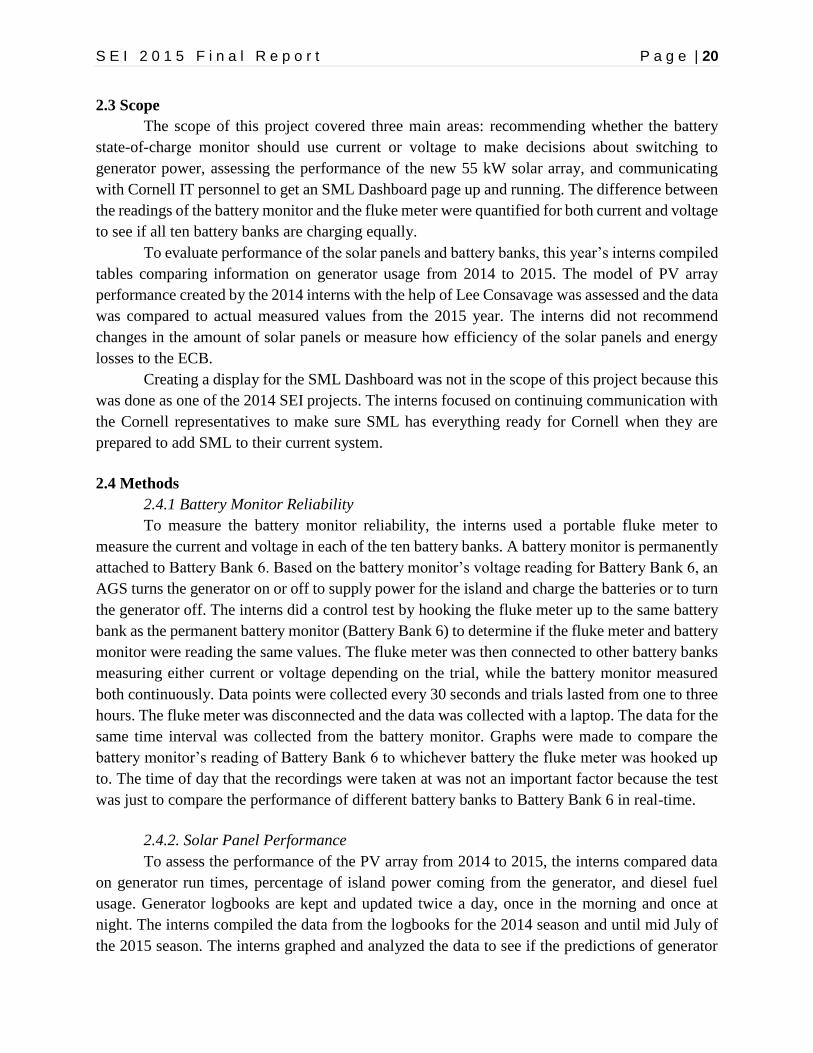
2.5.1 Battery Monitor Reliability
The current, in amperes, was measured with the fluke meter from all ten battery banks
against the current measured with the battery monitor on Battery Bank 6. Two trials were done for
measuring current to account for any error in case the meter had not been properly zeroed during
the first round of trials. A third trial was conducted to measure the difference in voltage between
the battery monitor and fluke meter in the ten battery banks to see if the voltage readings followed
a similar pattern. Since the data for Battery Bank 6 matched up closely for both the fluke meter
and the battery monitor during all three trials, the interns were able to assume that the fluke meter
readings were comparable to the battery monitor readings.
Figure 48: Battery Bank 6 Voltage
S E I 2 0 1 5 F i n a l R e p o r t P a g e | 22
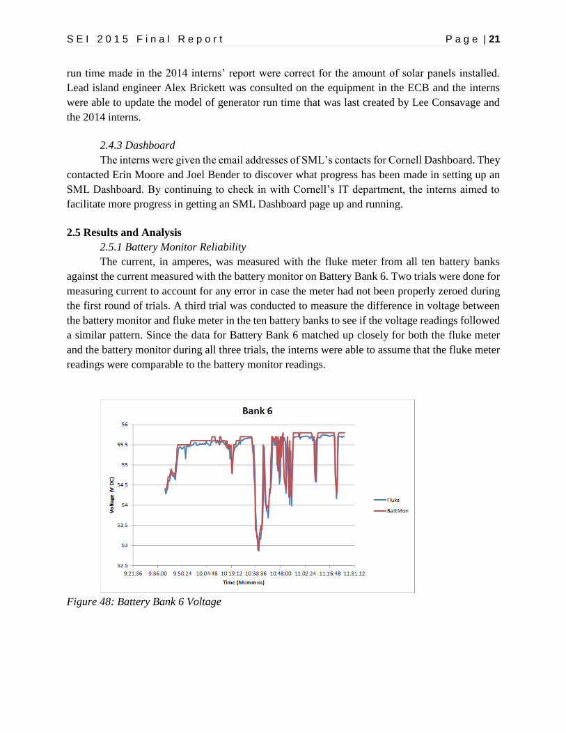
Figure 49: Battery Bank 6 Current
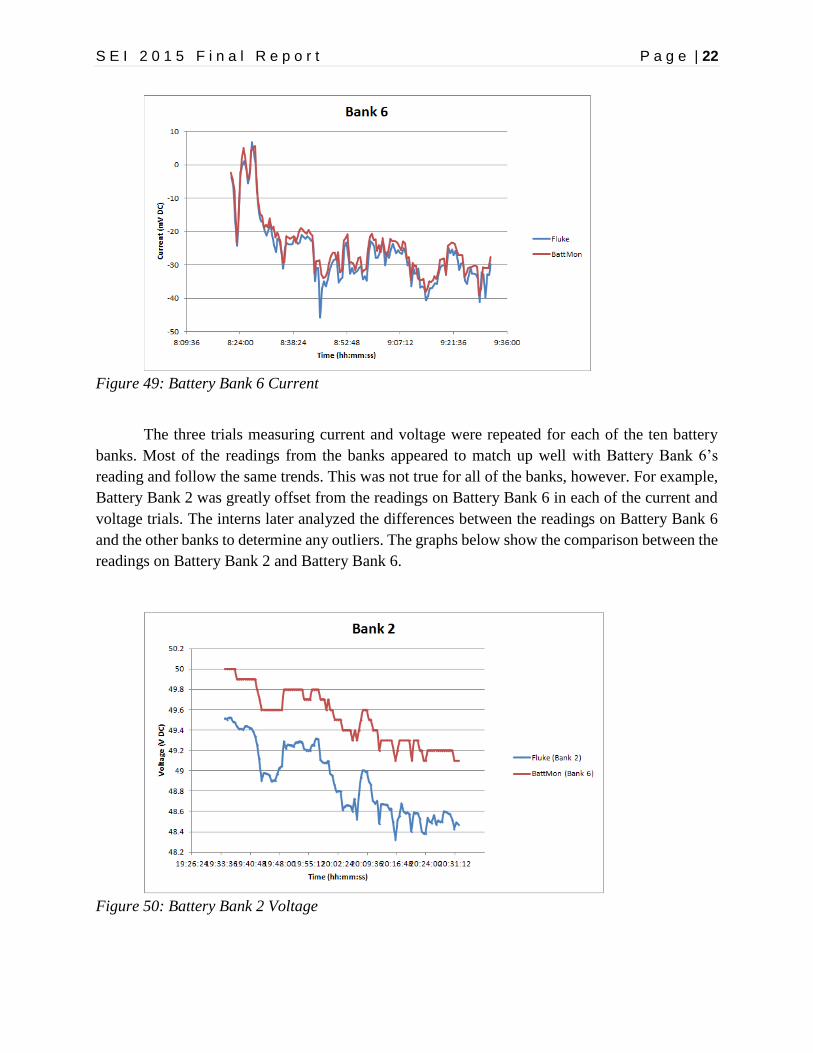
The three trials measuring current and voltage were repeated for each of the ten battery
banks. Most of the readings from the banks appeared to match up well with Battery Bank 6’s
reading and follow the same trends. This was not true for all of the banks, however. For example,
Battery Bank 2 was greatly offset from the readings on Battery Bank 6 in each of the current and
voltage trials. The interns later analyzed the differences between the readings on Battery Bank 6
and the other banks to determine any outliers. The graphs below show the comparison between the
readings on Battery Bank 2 and Battery Bank 6.
Figure 50: Battery Bank 2 Voltage

S E I 2 0 1 5 F i n a l R e p o r t P a g e | 23
Figure 51: Battery Bank 2 Current
The average differences measured in amps and in volts between the battery monitor
readings and the fluke meter readings were found for each trial. These differences were not
expressed as percent differences because current fluctuates between positive and negative values,
and percent differences do not work with numbers of opposite signs. By looking at the average
differences, the interns were able to roughly determine which banks may not be operating the same
as Battery Bank 6.
Table 26: Voltage Average Difference (V)
Bank 1 Bank 2 Bank 3 Bank 4 Bank 5 Bank 6 Bank 7 Bank 8 Bank 9 Bank 10
Trial 1 -0.1 -0.62 -0.06 -0.09 -0.03 -0.07 -0.12 -0.09 0.03 -0.12
Table 27: Current Average Difference (A)
Bank 1 Bank 2 Bank 3 Bank 4 Bank 5 Bank 6 Bank 7 Bank 8 Bank 9 Bank 10
Trial 1 -1.01 -21.11 -5.68 -2.48 -5.47 0.06 -2.66 1.18 10.05 5.74
Trial 2 0.06 14.94 0.25 -0.09 -3.81 -2.11 -0.85 -0.5 12.37 3.67
Based on these average differences tables, the interns noted that Battery Bank 2 and
Battery Bank 9 may not be charging and discharging the same as Battery Bank 6 because the
average differences were much higher than those of the other banks. The interns confirmed this
by performing an outlier calculation to determine which banks, if any, should be looked into for
efficiency. It was found that Battery Bank 2 was an outlier for all three trials and Battery Bank 9
was an outlier for one of the current trials.

S E I 2 0 1 5 F i n a l R e p o r t P a g e | 24
Figure 52: Voltage Average Differences
Figure 53: Current Average Differences
2.5.2 Solar Panel Performance
The 2014 model for generator run time based on PV array size included certain invalid
assumptions on system settings and island energy usage that made it difficult to compare actual
PV array performance to. Their model represented the 65 kW generator as being controlled by the
AGS, which is untrue. The 2014 model also included generator cycling, and assumed that the
generator was always producing maximum power output when in reality it is load dependent,
which caused the model to give inaccurate values for generator run times. Because of these
discrepancies, this year’s interns neglected the predictions made in 2014. The interns updated the
S E I 2 0 1 5 F i n a l R e p o r t P a g e | 25
2014 model to make it more accurate for future interns to use in their studies. For the purpose of
this study, the interns focused on comparing actual data from 2014 to 2015 based on generator
usage in order to evaluate the performance of the PV array.
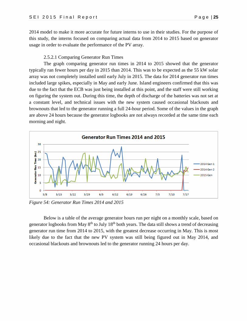
2.5.2.1 Comparing Generator Run Times
The graph comparing generator run times in 2014 to 2015 showed that the generator
typically ran fewer hours per day in 2015 than 2014. This was to be expected as the 55 kW solar
array was not completely installed until early July in 2015. The data for 2014 generator run times
included large spikes, especially in May and early June. Island engineers confirmed that this was
due to the fact that the ECB was just being installed at this point, and the staff were still working
on figuring the system out. During this time, the depth of discharge of the batteries was not set at
a constant level, and technical issues with the new system caused occasional blackouts and
brownouts that led to the generator running a full 24-hour period. Some of the values in the graph
are above 24 hours because the generator logbooks are not always recorded at the same time each
morning and night.
Figure 54: Generator Run Times 2014 and 2015
Below is a table of the average generator hours run per night on a monthly scale, based on
generator logbooks from May 8th to July 18th both years. The data still shows a trend of decreasing
generator run time from 2014 to 2015, with the greatest decrease occurring in May. This is most
likely due to the fact that the new PV system was still being figured out in May 2014, and
occasional blackouts and brownouts led to the generator running 24 hours per day.

S E I 2 0 1 5 F i n a l R e p o r t P a g e | 26
Table 28: Average Generator Hours Run per Night Each Month
2014 2015
May 15.08 9.82
June 14.59 12.31
July 12.54 11.17
2.5.2.2 Percent Power
Using information from the generator power logs and the total island power logs from 2014
and 2015, the interns looked at how the installation of the 55 kW solar array affected the percentage
of island power that came from the generator. It is important to note that the power from the old
green grid is not included in this data, which makes it appear that the renewable energy makes up
a smaller fraction of the total power than it actually does. The power percentages were found on
both a monthly breakdown and over the total measured time. The percentage of power supplied by
the generator decreased from 2014 to 2015 in each of the months that were evaluated. As shown
in the two pie charts, the summer of 2015 has shown a 6% decrease in power coming from the
generator compared to 2014.
Table 29: Percent Power from Generator
2014 2015 Difference
May 73.81% 65.52% -8.29%
June 70.92% 65.40% -5.52%
July 67.46% 61.11% -6.35%

S E I 2 0 1 5 F i n a l R e p o r t P a g e | 27
Figure 55: 2014 Island Power Breakdown
Figure 56: 2015 Island Power Breakdown
2.5.2.3 Diesel Fuel Consumption
By looking at diesel fuel logs, the interns were able to compare diesel fuel consumption
between 2014 and 2015. The interns were given the price per gallon of diesel as $3.70. Multiplying
the gallons of diesel used by the price per gallon gave the total diesel fuel costs for each year.

S E I 2 0 1 5 F i n a l R e p o r t P a g e | 28
Table 30: Diesel Fuel Consumption
Diesel Used (gal) Price per gallon ($/gal) Total Cost ($)
2014 1,924.7 3.70 7,121.39
2015 1,577.9 3.70 5,838.23
Based on these calculations, SML was able to reduce its diesel fuel consumption by 346.8
gallons from 2014 to 2015, the equivalent of $1283.18. This reduction in diesel fuel usage shows
that the new PV array is successfully reducing the load on the island generator.
2.5.3 Dashboard
Both Erin Moore and Joel Bender were contacted to see how much Cornell had progressed
in getting SML a Dashboard page. Joel replied, inquiring about what systems SML wanted to
include on the Dashboard display. The interns worked with Alex Brickett to determine what
systems would be the most important and easily understood information to show the public. The
interns told Joel to display the total real power, the energy from the PV array, and the battery
voltage.
2.6 Conclusions & Recommendations
2.6.1 Battery Monitor Reliability
Based on the data collected and calculations performed, the interns suspect that Battery
Bank 2 and Battery Bank 9 may not be functioning the same as the other batteries. There are a
variety of reasons that could be causing the battery banks to function differently. The interns did
not look into possible causes of this because it was outside of the scope of the project, but SML
staff or future interns should evaluate the performance of each of the batteries.
The interns recommend that SML staff change the AGS to make decisions based off of
current rather than voltage. They came to this conclusion for multiple reasons. First, the percent
state of charge can be determined instantaneously from the AGS because it just has to measure
what is going in and out of the battery at any given moment. This is not the case for voltage. To
accurately measure the voltage, the batteries must stand unused for several hours so that the voltage
can stabilize. The manufacturer says to let the voltage stabilize for 24 hours, but Star Island staff
stated that their batteries’ voltage stabilized after about 2 hours. This voltage stabilization test
should be performed to validate the interns’ suspicions of Battery Bank 2 and Battery Bank 9
charging differently than the other batteries. In addition, using voltage for the AGS when the wind
turbine is running does not work well because the energy produced is so variable. Based on the
accuracy of measuring state of charge and the ability to read the wind turbine output, SML should
switch the AGS to turning the generator on or off depending on current.

S E I 2 0 1 5 F i n a l R e p o r t P a g e | 29
2.6.2 Solar Panel Performance
Since the generator run time, the percentage of power produced by the generator, and the
diesel fuel consumption have all decreased since last summer, the interns have determined that the
solar panels are performing well. The batteries are usually fully charged by early afternoon, so
they are currently providing enough power to the system. When the batteries are fully charged,
they are in what is known as float mode. This is one of three main battery modes. These three
battery modes are defined below, thanks to assistance from Alex Brickett:
Bulk Stage (56.4V) - Lasts until approximately 90% of battery charge capacity. Full
current at a constant voltage. This stage puts as much energy into the batteries as possible.
Absorption (56.4V) - Gets the batteries to 100% charge without overcharging. Constant
voltage while lowering current.
Float (53.5V) - Idle, maintains the batteries at 100% charge.
When the batteries are idle in float mode, the excess power from the PV array is dissipated
as heat. To avoid wasting solar energy during the day, the interns recommend finding ways to
transfer more of the island load from the evening when the generator is running to the daytime
when the power is coming from the solar panels. The interns brainstormed ways to use less energy
at night and more during the day when the batteries are fully charged by the solar panels. These
ideas are listed in Project 5 - Electrical Load Profiles in section 5.7 Conclusions &
Recommendations. Additionally, settings in the ECB were recently changed so that the generator
now puts less power towards charging the batteries when it runs. The results of this system change
should be investigated once it has been in place for more time.
2.6.3 Dashboard
The interns believe that Cornell is close to having the SML Dashboard page setup because
Joel asked what systems would be the most important to display. If he is asking what should be
displayed, he is most likely prepared to display these things on the Cornell website. The interns
recommend that SML staff continue emailing Joel and Erin so that this project will become a
priority for Cornell IT and it will be completed before the next season. SML should also contact
UNH IT to try to get setup on their Dashboard as well.
2.7 References
“Installation and Operating Instructions For ABSOLYTE GP Batteries.” GNB Industrial Power,
2012. www.gnb.com

S E I 2 0 1 5 F i n a l R e p o r t P a g e | 30
Project 3 - Saltwater Pump Efficiency
3.1 Background
Saltwater must be reliably distributed around the island to various sea tables used for
biological research to maintain sea-like conditions for the organisms to survive. The saltwater is
also used for all the island’s fire hoses, therefore reliability of flow is extremely important for
island safety. The current salt water pump is a Goulds 3656 1 ½ x 2-8 G. It continuously uses the
same amount of electricity regardless of the flow rate. The sea tables and fire hoses are not all
always being used and this creates a variation in flow. The variation in flow does not create a
variation in electricity draw which wastes electricity. By altering the saltwater pump system and
reducing its load on the electrical system, the sustainable energy sources will be able to fulfill more
of the energy demands of the island and less energy from the diesel generator will be required. A
new system will need to be compatible with the island’s other current systems and equipment. The
location of the pump will require a sturdy and ocean resistant design to prevent failures and must
also have a reasonable cost of implementation, operation, and maintenance.
Figure 57: GIS Graphic of Current Saltwater System
3.2 Purpose
Provide a comparison study of different saltwater pumps and recommend the one which
will increase island electricity efficiency. This will further allow SML to attain its goal of operating
with sustainable energy.

S E I 2 0 1 5 F i n a l R e p o r t P a g e | 31
3.3 Scope
The interns examined the current saltwater pump operating system for electrical draw and
flow rate. The island’s saltwater needs were studied in order to recommend a viable solution. Pump
replacements were recommended which included a smaller centrifugal pump in the current pump
location and a submersible pump. Recommendations were made to further research variable
frequency drives (VFD) in order to reduce the electrical draw of the pump.
3.4 Methods
3.4.1 Electrical Energy Draw
Using the Eagle 440 electricity meter, the energy usage of the current saltwater pump was
recorded over the course of 15 hours. To validate this value, the electricity used by the current
pump was monitored for two trials by turning the pump on and off and observing the change in
total island power. The energy difference was observed from two different locations on the island.
One meter was located in the generator room, which monitors total island energy passing through
the generator room equipment. The other meter was located in the Energy Conservation Building,
which measures energy used by the entire island system leaving that building. The generators were
not running during either test.
3.4.2 Maximum Flow Rate
The maximum flow of the saltwater system was determined by turning on all of the sea
tables, with the exception of the Grass Lab’s table, and two fire hoses. The interns were advised
by SML staff not to include the table in the Grass Lab because it has not been used for a class in
several years. During this test, SML staff recommended to test using two fire hoses, because during
an emergency only two Above Low Tide
Another variable that needed to be measured was the elevation of the pump from the ocean
surface. To get the largest hoses were likely to be used at any given time. The flow meter on the
pump was examined when all these systems were on for maximum flow.
3.4.3 Elevation of Pump
The interns measured elevation at two different low tide times. They used mobile altimeter
software which utilized GPS to measure the change in elevation from the low tide dock to the
pump. This was repeated four times in order to get an averaged value.
3.4.4 Pump and System Sizing
The current pump’s manufacturer label was recorded to gain information from the
manufacturer. By using the Bernoulli equation, the system curve was determined. This curve was
compared to pump curves from various manufacturers. Several types of pumps were researched,
and replacement centrifugal and submersible pump types were researched. Pumps that had a lower
horsepower than the current model were selected.

S E I 2 0 1 5 F i n a l R e p o r t P a g e | 32
3.5 Results & Analysis
3.5.1 Electrical Draw of Saltwater Pump
The electrical draw of the saltwater pump was calculated in two ways. First, the Eagle 440
measured the electrical draw of the system as 3.5 kW over an average of fifteen hours. The interns
validated this number by manually turning the pump off for a short time while the change in energy
was recorded. The manual shut down showed that the draw from the pump in the generator room
was greater than that in the ECB. This was confusing, because the values should theoretically be
the same. The value that was recorded by the ECB for energy draw was probably the more accurate
measurement, because it was closest to the Eagle 440 data average.
Figure 58: Recorded Energy Use of Salt Water Pump from Manual Shut Off
S E I 2 0 1 5 F i n a l R e p o r t P a g e | 33
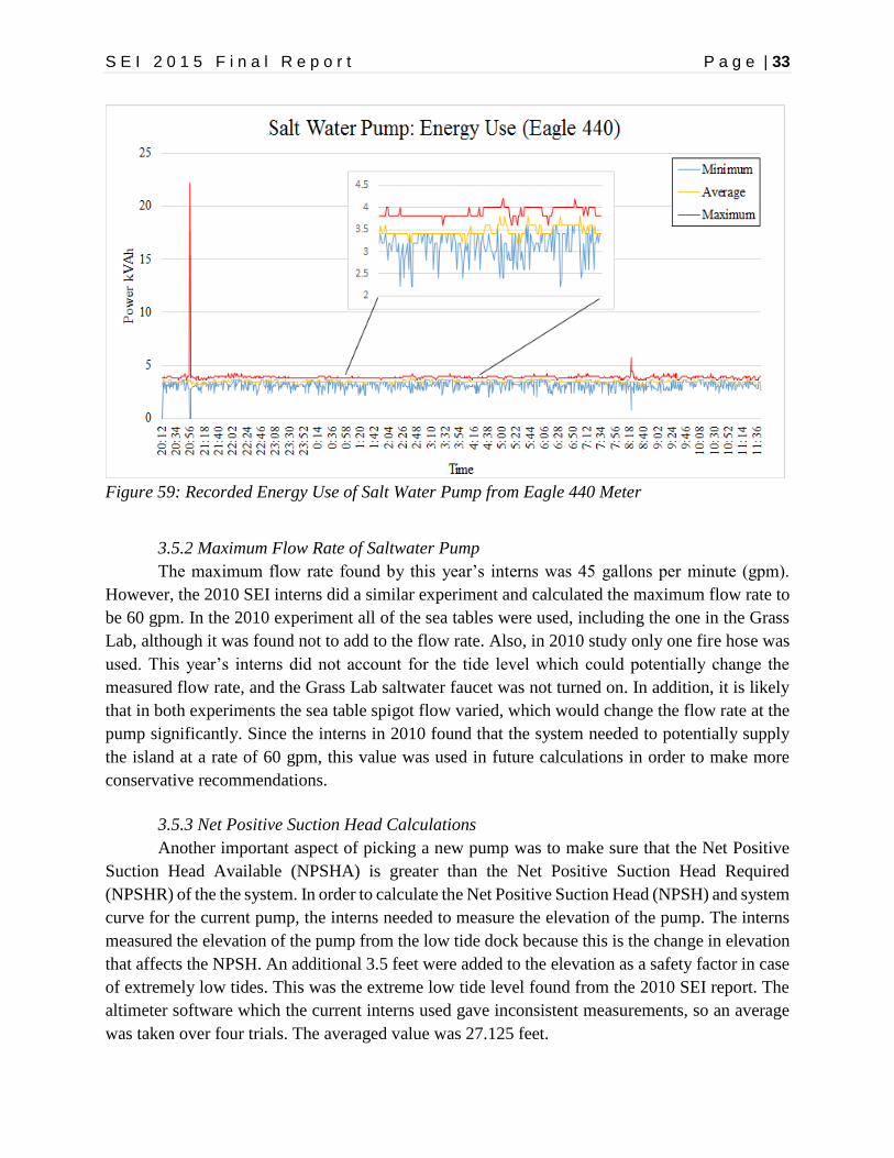
Figure 59: Recorded Energy Use of Salt Water Pump from Eagle 440 Meter
3.5.2 Maximum Flow Rate of Saltwater Pump
The maximum flow rate found by this year’s interns was 45 gallons per minute (gpm).
However, the 2010 SEI interns did a similar experiment and calculated the maximum flow rate to
be 60 gpm. In the 2010 experiment all of the sea tables were used, including the one in the Grass
Lab, although it was found not to add to the flow rate. Also, in 2010 study only one fire hose was
used. This year’s interns did not account for the tide level which could potentially change the
measured flow rate, and the Grass Lab saltwater faucet was not turned on. In addition, it is likely
that in both experiments the sea table spigot flow varied, which would change the flow rate at the
pump significantly. Since the interns in 2010 found that the system needed to potentially supply
the island at a rate of 60 gpm, this value was used in future calculations in order to make more
conservative recommendations.
3.5.3 Net Positive Suction Head Calculations
Another important aspect of picking a new pump was to make sure that the Net Positive
Suction Head Available (NPSHA) is greater than the Net Positive Suction Head Required
(NPSHR) of the the system. In order to calculate the Net Positive Suction Head (NPSH) and system
curve for the current pump, the interns needed to measure the elevation of the pump. The interns
measured the elevation of the pump from the low tide dock because this is the change in elevation
that affects the NPSH. An additional 3.5 feet were added to the elevation as a safety factor in case
of extremely low tides. This was the extreme low tide level found from the 2010 SEI report. The
altimeter software which the current interns used gave inconsistent measurements, so an average
was taken over four trials. The averaged value was 27.125 feet.

S E I 2 0 1 5 F i n a l R e p o r t P a g e | 34
Table 31: Elevation Difference Between Low Tide and Pump
Trial Date/Time/Tide Elevation (ft) Extreme Low Tide Elevation (ft)
1 7/17 07:15 -0.3ft 20.5 24
2 7/17 07:15 -0.3ft 30 33.5
3 7/17 07:15 -0.3ft 31 34.5
4 7/22 10:00 0.8ft 13 16.5
Ave 23.625 27.125
With this averaged elevation and other variables, the interns used the below equation to
calculate the NPSHA for the current system. They found the NPSHA to be 5.35 feet. The validity
of this value is uncertain, as most pumps have an NPSHR of about 10 to 20 feet. The interns this
year compared their equation to the 2010 interns’ equation. The 2010 calculations did not show
where their variables’ values came from. Their published answer does not add up to their other
variables. Because of this, this year’s interns disregarded the 2010 calculated NPSHA value.
Since the interns did not think their calculation or the 2010 calculation were correct, they
looked at the current pump curve to estimate NPSHA. At the existing operating point, the NPSHR
for the centrifugal pump was eight feet. Tom Ballestero provided the below equations which add
a few feet as a safety factor to NPSHR, which yields NPSHA. The interns used this calculation to
find that NPSHA must be at least 11 feet. These values confirmed the interns’ suspicions that the
NPSHA calculation gave an inaccurate answer. The interns recommend that the actual NPSHA be
thoroughly calculated.
The interns were concerned that by using the NPSHA value which was too low the
recommended pumps would not fit the island’s needs. The interns decided the best way to combat
this problem would be to assume NPSHR for a new system must be eleven feet or less. By doing
this, the recommended pump will be able to meet the island’s needs.
Equation 8: Net Positive Suction Head
Variable Definitions:
HA = Atmospheric pressure at sea level
HZ = Change in elevation
Q = Flow (a range of gpm from 0 to 60)
A = Cross sectional area of intake pipe
Dintake = Diameter of intake pipe
Hf = Friction head loss

S E I 2 0 1 5 F i n a l R e p o r t P a g e | 35
Hvp = Vapor pressure of seawater
Equation 9: Net Positive Suction Head Apparent and Required
3.5.4 System Curve Calculations
In order to calculate the system curve, which is a representation of flow and dynamic head
of the system, the equation below was used. This equation uses two pipes to represent the entire
system. The first pipe is the intake pipe which travels from the ocean to the pump. The second pipe
connects the salt water system from Palmer Kinne to the Kiggins Commons sea tables. The second
pipe was chosen to represent the system because it is located furthest away from the pump, with
the exception of the Grass Lab’s table, but this table was not included in the other analyses.
Equation 10: System Curve
The system curve was plotted from 0 to 60 gpm to create the following pump curve.
Because the Hp equation does not include the total head loss and friction loss due to bends and
pipes for every pipe in the system, the total losses were added after. Due to lack of time for the
interns to accurately account for all the bends, fittings, valves, and pipe changes in the system, the
total losses were found by using the highest total dynamic head from the Hp system curve
calculation. The highest total dynamic head from the Hp system curve calculation was 36.5 feet.
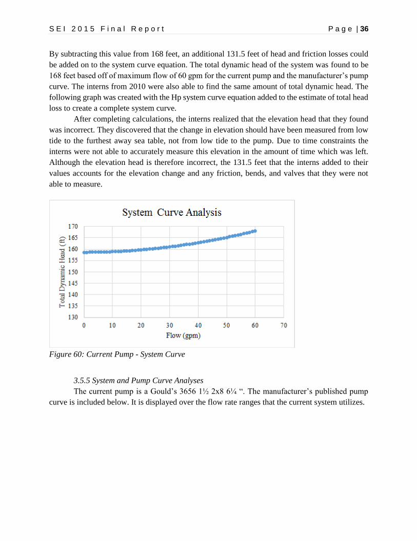
S E I 2 0 1 5 F i n a l R e p o r t P a g e | 36
By subtracting this value from 168 feet, an additional 131.5 feet of head and friction losses could
be added on to the system curve equation. The total dynamic head of the system was found to be
168 feet based off of maximum flow of 60 gpm for the current pump and the manufacturer’s pump
curve. The interns from 2010 were also able to find the same amount of total dynamic head. The
following graph was created with the Hp system curve equation added to the estimate of total head
loss to create a complete system curve.
After completing calculations, the interns realized that the elevation head that they found
was incorrect. They discovered that the change in elevation should have been measured from low
tide to the furthest away sea table, not from low tide to the pump. Due to time constraints the
interns were not able to accurately measure this elevation in the amount of time which was left.
Although the elevation head is therefore incorrect, the 131.5 feet that the interns added to their
values accounts for the elevation change and any friction, bends, and valves that they were not
able to measure.
Figure 60: Current Pump - System Curve
3.5.5 System and Pump Curve Analyses
The current pump is a Gould’s 3656 1½ 2x8 6¼ “. The manufacturer’s published pump
curve is included below. It is displayed over the flow rate ranges that the current system utilizes.
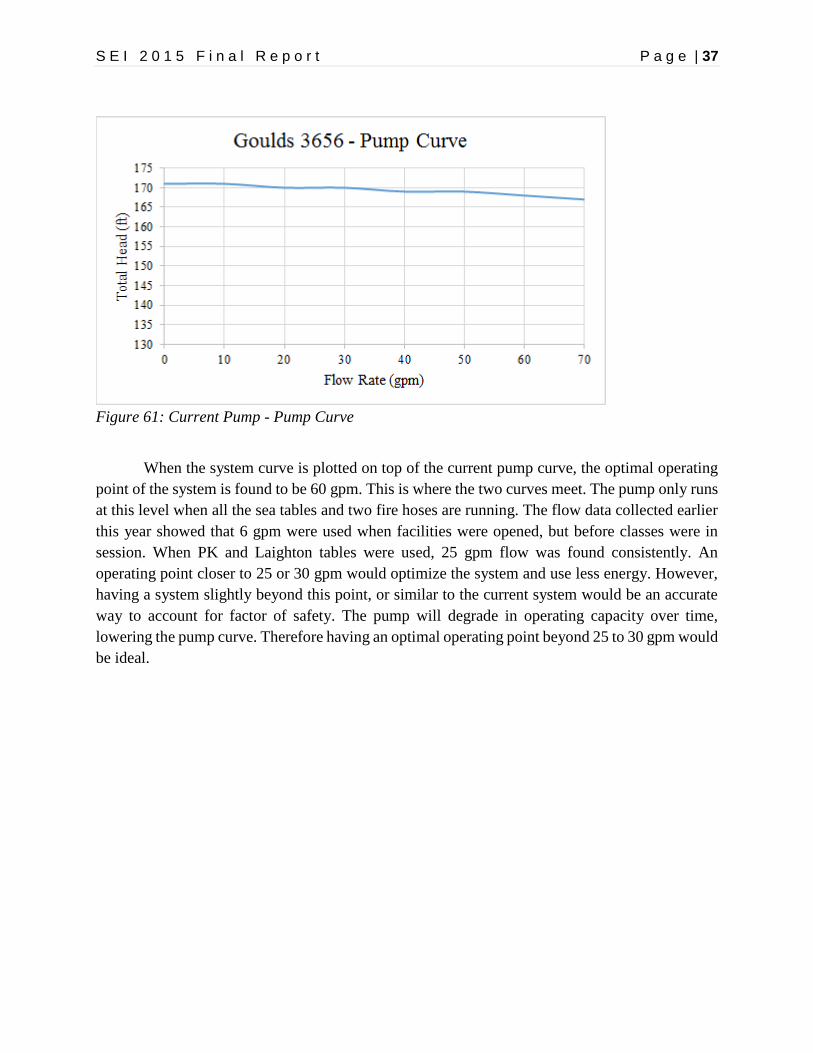
S E I 2 0 1 5 F i n a l R e p o r t P a g e | 37
Figure 61: Current Pump - Pump Curve
When the system curve is plotted on top of the current pump curve, the optimal operating
point of the system is found to be 60 gpm. This is where the two curves meet. The pump only runs
at this level when all the sea tables and two fire hoses are running. The flow data collected earlier
this year showed that 6 gpm were used when facilities were opened, but before classes were in
session. When PK and Laighton tables were used, 25 gpm flow was found consistently. An
operating point closer to 25 or 30 gpm would optimize the system and use less energy. However,
having a system slightly beyond this point, or similar to the current system would be an accurate
way to account for factor of safety. The pump will degrade in operating capacity over time,
lowering the pump curve. Therefore having an optimal operating point beyond 25 to 30 gpm would
be ideal.

S E I 2 0 1 5 F i n a l R e p o r t P a g e | 38
Figure 62: Operating Point of Current System
3.6 Conclusions & Recommendations
3.6.1 Replacement Options & Cost Analysis
Two pumps have been recommended by the interns. One is a centrifugal pump, like the
current pump, and the other is a submersible pump. Both pumps have the potential to decrease the
electrical draw of the island. The centrifugal pump is from Grundfos; its model name and number
are CM10-3A-S-A-E-AQQE 97524349. The submersible pump is also from Grundfos; its model
name and number are 60S50-7-35707951.
Table 32: Cost Analysis of Saltwater Options
Option Purchase
Cost ($)
kWh/season
(120 days)
Cost of
Operation
$/season
Cost
Reduction
($)/season
Diesel Fuel
Reduction
(gal)/season
Payback
(seasons)
Current
Pump
0.00 10266.24 5543.77 0.00 0.00 NA
Centrifugal 846.56 1384.77 747.77 4796.00 794.41 0.18
Submersible 1847.00 4609.32 2489.03 3054.74 505.99 0.60
Both new pump options require fewer horsepower; the centrifugal pump is 5.36HP and the
submersible pump is 4.96HP. The centrifugal pump replacement option would reduce energy cost
of use by $4796, which is a larger cost reduction than the submersible pump’s of $3055.

S E I 2 0 1 5 F i n a l R e p o r t P a g e | 39
3.6.2 Submersible Replacement Pump Analysis
The main benefit of the submersible pump is that the NPSHR can be negated. Because the
pump is underwater, the pump does not need suction to pull the water into the pipe. The cost of a
submersible pump, which is $1847, would be paid back in less than one season. However, there
are many drawbacks to the submersible pump. First, the pump would need to be in a sleeve to
create adequate flow for the system. Without a sleeve to mimic the conditions of a groundwater
well, the large holding tank, or ocean, can easily damage the pump. This recommendation was
given to the interns by pump technicians at both Goulds and Grundfos. Additional expenses and
time commitments are required for the submersible pump installation. SML staff would need to
send divers into the water several times in order to secure the pump and its sleeve. Divers will also
be needed for any pump maintenance, which will be more time consuming and difficult than
performing maintenance above water. There is also a concern of a Variable Frequency Drive
(VFD) causing harmonics in the system because it is far away from the submersible pump.
Harmonics are potentially damaging because they can increase the amount of current needed to
make the motor run at the same speed as it would without harmonics, causing the motor to overheat
and waste energy. SML would need to work with a pump distributor to match a VFD with this
type of pump.
The submersible pump option when graphed with the system curve creates an optimal
operating point of 60 gpm, which is the same as the current system. When the system is at 25 to
30 gpm, the available total head is much higher. This is also similar to the current system, because
it operates significantly under the pump curve. However, the submersible pump would operate at
a lower efficiency than the current system. This could be remedied by installing a VFD, and the
pump would still be reducing energy costs and usage from the current system.
Figure 63: Analysis of Submersible Pump Option with System Curve

S E I 2 0 1 5 F i n a l R e p o r t P a g e | 40
3.6.3 Centrifugal Replacement Pump Analysis
The interns recommend installing a new, smaller centrifugal pump rather than a new
submersible pump. The main reason for this is that a smaller centrifugal pump will operate with
the current system’s infrastructure. This pump will not need a sleeve, and it will be easier to
perform maintenance on since it will not be under water. It is also less expensive than the
submersible pump and saves more energy per season. If a VFD is installed, it will be less likely
for harmonics to occur because it can be closer in proximity to the motor and the pump. A pump
distributor should be contacted to find out what VFD would work best with this system.
This centrifugal pump curve when graphed with the system curve yields an optimal
operating point around 65 gpm. This pump installation would allow for the needs of the system to
be adequately matched. The pump curve is larger than absolutely necessary to allow for pump
aging over time. As the pump ages, the pump curve will be lowered. With this design, the pump
will be able to meet SML’s requirements for a longer period of time. While the pump will be
operating at a lower efficiency when using a flow rate of 30 gpm, a VFD may rectify this problem.
The pump will still be able to reduce energy costs and use compared to the current system.
Figure 64: Analysis of Centrifugal Pump Option with System Curve
3.6.4 Net Positive Suction Head Recommendations
NPSHA must be equal to or greater than NPSHR. Assuming NPSHA is actually eleven
feet, the recommended smaller centrifugal pump will not be able to pump water if the flow is at
60 gpm. The interns doubt this will be a problem, however, because the interns this year were only
able to get a max flow rate of 45 gpm. Therefore, according to this lower flow rate, the NPSHR
will be closer to eleven feet, which should meet the necessary demands. The NPSHR value can be
negated for the submersible pump, so this is only an issue for the replacement centrifugal pump.

S E I 2 0 1 5 F i n a l R e p o r t P a g e | 41
Table 33: Net Positive Suction Head
Option NPSHR (ft) @ 60 gpm NPSHR (ft) @ 30 gpm
Current System 8 8
Centrifugal 16 5
Submersible NA NA
The interns doubt that the calculations done thus far to calculate NPSHA are correct. Before
purchasing a new pump, a pump expert should be contacted to confirm the value of NPSHA. If
this value is not confirmed, there is a risk in purchasing a pump with a value of NPSHR greater
than the NPSHA, which would not be strong enough to bring water up through the pipes. Until
there is an accurate measurement for this variable, SML should stay with the current pump.
One possibility other than installing a new pump is to move the pump house closer to mean
high tide level. The interns questioned Lee Consavage about this. He advised the interns that this
may not make much of a difference because the total head of the system will remain the same.
What would change with moving the pump location is the NPSHA. The closer the pump is to the
water, the higher the value of NPSHA will be because there is less distance for the pump to pull
water from. While the interns had problems calculating NPSHA, if the pump house was lowered
then this variable would be less of a concern. However, there are other concerns for moving the
pump closer to the water. There is a cost involved with building the new pump house and installing
new piping. Also, in the case of an extremely high tide or a large storm, the pump house will be
more likely to flood or be damaged. Because of these reasons, the interns do not recommend for
the pump house to be moved down to a lower elevation.
3.6.5 Variable Frequency Drive Recommendation
The installation of a VFD will help reduce the electrical draw of whichever pump is
installed. The pump that is installed, whether it is the current pump or one of the recommended
pumps, needs to be sized for the maximum flow. Since this is rarely the case, a VFD can be
installed with the pumping system to lower the electrical draw of the system. Without a VFD, a
pump will constantly use the same amount of energy regardless of the demand. With the VFD,
however, the pump will only use the amount of energy needed for the demand at any given
moment. A VFD helps to save energy whenever the demand of the system is lower than the
maximum load. The interns asked the Grundfos technician about VFDs, and the technician highly
recommended installing one with the current or a new pumping system. The technician said that
either of the recommended pumps will operate with a VFD, but a pump distributor should be
contacted to ensure the VFD will operate at maximum efficiency with the rest of the system. SML
should contact a pump distributor nearby to find a VFD that works with the current pump or with

S E I 2 0 1 5 F i n a l R e p o r t P a g e | 42
a new pump so that the saltwater pump will draw as little electricity as possible. The numbers of
two pump distributors are included in the Appendix.
3.7 References
The Engineering Tool Box.
http://www.engineeringtoolbox.com/
Average Ocean Temperatures for Maine & New Hampshire. “Current Results.”
http://www.currentresults.com/Oceans/Temperature/maine-new-hampshire-average-water-
temperature.php

S E I 2 0 1 5 F i n a l R e p o r t P a g e | 43
Project 4 - Electrical Transformer Study
Key terms for this section:
Real power - The power demand of a system, given in kW*.
Reactive power - Power consumed by inductance that must be supplied by the generator
in addition to real power, given in kVAR*.
Apparent power - Total power the generator must put into the system to account for some
of the power being lost due to operation, given in kVA*.
Measured Load - Measured power at the output of the transformer.
Percent Load - Ratio of measured load to the nameplate rating of the transformer.
Coil Loss - Losses in the form of heat from the coil windings, dependent on load.
Core Loss - Losses caused by magnetizing current that energizes the transformer core,
constant and not dependent on load.
*kW, kVAR and kVA are equivalent units, they are written differently to distinguish
between what type of power is being discussed.
4.1 Background
There is a network of dry type electrical transformers that transmit power to the buildings
at SML. These transformers are used to step the voltage up or down as needed when electricity
enters each building. The current system may be inefficient and result in energy losses. An
assessment of the transformer network on Appledore should determine if any changes can be made
to reduce power losses while still providing enough power to buildings.
4.2 Purpose
A professional electrician advised SML that the current transformer network may be
wasting electricity. Now that SML has installed the maximum number of recommended solar
panels, the focus is on energy conservation measures to further reduce the load on the island
generator. By doing an assessment of the losses with and without transformers and looking at the
efficiencies of each transformer, SML may be able to reduce its power losses.
4.3 Scope
The interns created tables comparing power losses with the current transformers to losses
if the transformers were to be removed. Based on average measured loads for various transformers
on the island and manufacturer data for transformer losses, the transformer efficiencies were
calculated. These comparison tables were analyzed, and recommendations for changes to the
current transformers network were included in this project.

S E I 2 0 1 5 F i n a l R e p o r t P a g e | 44
4.4 Methods
4.4.1 Preliminary Research
Extensive research of the current transformer network was required in order to make
recommendations based on losses and efficiency. The transformer manufacturer labels in each
building were examined and used to find necessary information including power, impedance, and
high voltage current. Square D Company, the transformer manufacturer, was contacted to obtain
coil losses and core losses of each type of transformed owned by SML. Using these transformer
specifications, equations provided by Unitil representatives and Lee Consavage, and SML’s
Geographical Information Systems (GIS), an analysis of line losses and efficiency for each
transformer was compiled.
4.4.2 Eagle 440 Meter
The power outputs of several transformers were measured using a power meter called the
Eagle 440. Ross Hansen hooked the Eagle 440 meter up to each transformer for approximately a
24-hour period so that an average measured load could be obtained. The transformers located in
Bartels, Kiggins, Kingsbury House, Laighton, Utility Building, and ECB were all measured. The
interns worked with ProVision software to download and analyze the output data from the meter.
This data included net power consumption over the duration of time, as well as graphs and tables
of the output power in minute intervals. The Eagle 440 measured real power, reactive power, and
apparent power. These terms are defined at the beginning of this project. The interns looked at
apparent power because that is the power that is actually being put into the system.
4.4.3 Line Losses
With the help of Lee Consavage, the interns were able to create a table of line losses from
the ECB to each building for two scenarios: with and without transformers. The line losses were
based on cable lengths, the voltage that the electricity was transmitted at, and the effective Z value
of the cables that were found in a table provided by Consavage. The interns used the SML GIS
database to determine cable lengths for the buildings.
4.4.4 Transformer Efficiencies
After the Eagle 440 data was downloaded in ProVision, the average measured load for each
building was calculated. This measured load was obtained by dividing the Net Apparent Power
Consumed in kVAh by the number of hours that the meter was hooked up to the transformer. These
measured loads were compared to the nameplate rating of the transformers to calculate percent
loads on each transformer.
Coil and core losses are specific to each transformer type and these transformer losses vary
with percent load. With newer transformers, these losses are published for different percent loads.
Most of SML’s transformers, however, are older and do not have these values published. The
interns found 0% load losses and 100% load losses for each of the transformers from a Square D
Company technician. They fit an exponential curve to these two points to obtain an equation for
finding the losses specific to each building’s load. To make sure an exponential curve would be an

S E I 2 0 1 5 F i n a l R e p o r t P a g e | 45
accurate curve fitting for the transformers, published load losses from other transformers were
plotted and fit with exponential curves. In each case, the correlation value was over 99%. Because
of this, the interns felt confident using exponential curves to fit the transformer losses at percent
loads for the transformers with missing data points.
With the measured load from the Eagle 440 meter and the load losses specific to each
transformer’s load, the interns were able to calculate the percent efficiencies of each of the
transformers.
4.5 Results & Analysis
The interns were given two different equations to calculate transformer losses. One of these
equations was from Lee Consavage, and it took into account the impedance value of the
transformer but not the percent load. The impedance value was obtained from the transformer
label. The second equation was from Unitil, and it took into account the percent load of the
transformer but not the impedance value. The percent load calculation includes the actual load that
the Eagle 440 power meter collected at each location divided by the total power that the
transformer is rated for. Both equations were used and their answers were compared. In both cases,
the total power loss was greater if the transformers in Bartels, Laighton, and K-House were
removed.
Table 34: Losses Based on Transformer Impedance
Building: Impedance Value (%)
Total Power Loss
Remove Transformer
(kW)
Total Power Loss Keep
Transformer (kW)
Bartels 4.40% 1.4441 0.857
Laighton 5.10% 1.0425 0.993
K-House 4.40% 1.4698 1.004
Table 35: Losses Based on Percent Load
Building: Percent Load
Total Power Loss Remove
Transformer (kW)
Total Power Loss Keep
Transformer (kW)
Bartels 0.49% 1.4441 1.134
Laighton 2.90% 1.0425 0.4964
K-House 0.77% 1.4698 1.0087
The interns were also given an equation for transformer efficiency from Unitil. The
measured loads are recorded in the table below. The total losses at the percent load were found.
Using the Eagle 440 data for measured load as the power out (Pout) and the total losses at the
percent load, the transformer efficiency was found.

S E I 2 0 1 5 F i n a l R e p o r t P a g e | 46
Equation 11: Transformer Efficiencies
Table 36: Transformer Efficiencies
Building Maximum
Load
(kVA)
Measured
Average Load
(kVA)
Transformer
Size (kVA)
Total Losses at
Percent Load (kW)
Transformer
Efficiency
Bartels 3.8 0.148 30 0.326 31.28%
Kiggins 22.6 6.422 45 0.313 95.35%
ECB 40.2 23.120 45 0.630 97.35%
Laighton 2.4 0.869 30 0.245 78.01%
K-House 3.2 0.230 30 0.330 41.07%
Utility 13.2 0.530 45 0.238 69.01%
The maximum load on each building was also found from the Eagle 440 data. This value
should be used if SML wants to replace any of the transformers with one that is more suited for
the load of that building. An example of the data from the Eagle 440 that the maximum load was
determined from is shown below.
Figure 65: Energy Conservation Building Apparent Power

S E I 2 0 1 5 F i n a l R e p o r t P a g e | 47
The interns used this data in order to find the maximum apparent power value over the time
interval. It is recommended to use a factor of safety when sizing a transformer based on this
maximum power value because it was only taken over approximately a 24-hour period and that
may not have been the day with the highest load on the building.
4.6 Conclusions & Recommendations
The interns determined that the transformers in Bartels, Laighton, and Kingsbury House
should not be removed. The line losses from transporting the power to the buildings at lower
voltages would be greater than the power losses from having the transformers.
The interns recommend investigating transformers that have efficiencies below 90%. SML
should evaluate the possibility of replacing the Bartels, Kiggins, Laighton, K-House, and Utility
Building transformers to increase the transformer efficiency. This could mean finding a more
appropriately sized transformer so that the percent load is higher, or researching newer, more
efficient models. A cost analysis should be done to calculate power loss reductions and cost
reductions to assess whether it is worth purchasing new transformers. Before a decision is made
on what size transformer to replace the current ones with, it may be beneficial to take more
measurements of the maximum loads of each building to ensure the maximum load will be less
than the rated load of the transformer.
4.7 References
"Table 9 Alternating-Current Resistance and Reactance for 600-Volt Cables, 3-Phase, 60 Hz,
75°C (167°F) — Three Single Conductors in Conduit." National Electrical Code. 2011 ed. N.p.:
n.p., n.d. N. pag. Web. 26 July 2015. <http://www.inw-
training.com/joomla1/images/2008NEC/ch9t9.pdf>.
Eisfeller, Justin, and Andrew Jacobs. 'Basic Calculations And Protection Overview'. 2015.
Presentation.
Jacobs, Andrew. 'Transformer Basics And Efficiency Calculation'. 2015. Presentation.

S E I 2 0 1 5 F i n a l R e p o r t P a g e | 48
Project 5 - Electrical Load Profiles
5.1 Background
In order to fully understand SML’s electrical load, individual buildings’ electrical load
profiles need to be created. By understanding the electrical load of the island, better conservation
measures can be incorporated. Additionally, SML wants to eliminate the possibility of the inverters
in the ECB exceeding its maximum load of 36 kW. SML would be able to better plan the size and
types of programs by knowing the capabilities and limits of their facilities. In addition to creating
load profiles to target electrical loads that can be lowered, an estimation of energy use per person
will aid in planning and scheduling what the island can support each season.
5.2 Purpose
Document the electrical load of buildings and large appliances so that information on island
electricity use is available. Provide recommendations on ways to decrease electrical use in order
to lower energy generation needs.
5.3 Scope
The interns measured electrical load profiles of as many buildings and large appliances as
possible. These load profiles were compiled into graphs for comparison. The interns estimated
total electrical load by building by researching wattage of every electrical appliance. Electrical
conservation strategies were suggested based on the load profiles and appliance audit results.
5.4 Methods
5.4.1 Eagle 440 Transformer Readings By Building
The transformer output power data recorded by the Eagle 440 for the transformers in
Bartels, Kiggins Commons, Energy Conservation Building, Laighton, and Kingsbury House were
used as an electrical load profile to compare to the theoretical load profiles. The power meter was
also used to record the power used by the salt water pump, and the freezer and refrigeration system
in Kiggins. The Eagle 440 measured power data in each location for approximately 24 hours.
Buildings were grouped into categories of similar electricity usage to assist with electrical load
monitoring.
5.4.2 Electrical Appliance By Building
All electrical appliances in each building on the island were recorded to create a theoretical
calculation of the electrical load in each building. Wattage of each appliance was researched
through manufacturer information and hours of use for each season were estimated. With that
information, an estimate of electrical energy use for each building was created.
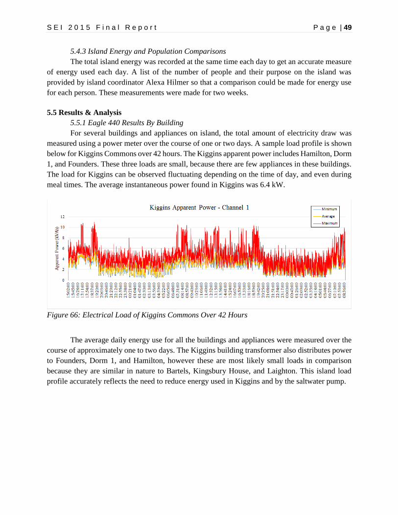
S E I 2 0 1 5 F i n a l R e p o r t P a g e | 49
5.4.3 Island Energy and Population Comparisons
The total island energy was recorded at the same time each day to get an accurate measure
of energy used each day. A list of the number of people and their purpose on the island was
provided by island coordinator Alexa Hilmer so that a comparison could be made for energy use
for each person. These measurements were made for two weeks.
5.5 Results & Analysis
5.5.1 Eagle 440 Results By Building
For several buildings and appliances on island, the total amount of electricity draw was
measured using a power meter over the course of one or two days. A sample load profile is shown
below for Kiggins Commons over 42 hours. The Kiggins apparent power includes Hamilton, Dorm
1, and Founders. These three loads are small, because there are few appliances in these buildings.
The load for Kiggins can be observed fluctuating depending on the time of day, and even during
meal times. The average instantaneous power found in Kiggins was 6.4 kW.
Figure 66: Electrical Load of Kiggins Commons Over 42 Hours
The average daily energy use for all the buildings and appliances were measured over the
course of approximately one to two days. The Kiggins building transformer also distributes power
to Founders, Dorm 1, and Hamilton, however these are most likely small loads in comparison
because they are similar in nature to Bartels, Kingsbury House, and Laighton. This island load
profile accurately reflects the need to reduce energy used in Kiggins and by the saltwater pump.

S E I 2 0 1 5 F i n a l R e p o r t P a g e | 50
Figure 67: Average Daily Energy Use
5.5.2 Electrical Appliance By Building
The following table is an excerpt from the electrical appliance audit that was done for each
building on the island. The full audit includes each appliance, its wattage, and an estimate of the
amount of time it is in use each season. These numbers can then be used to determine how much
electricity each appliance uses. When all the buildings are compared, a second island electrical
load profile can be compiled from appliances and estimates of their use each season.
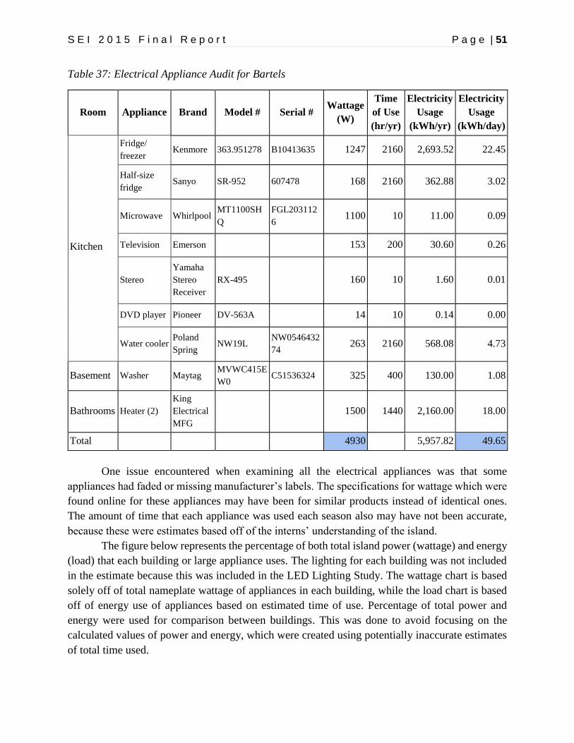
S E I 2 0 1 5 F i n a l R e p o r t P a g e | 51
Table 37: Electrical Appliance Audit for Bartels
Room Appliance Brand Model # Serial # Wattage
(W)
Time
of Use
(hr/yr)
Electricity
Usage
(kWh/yr)
Electricity
Usage
(kWh/day)
Kitchen
Fridge/
freezer Kenmore 363.951278 B10413635 1247 2160 2,693.52 22.45
Half-size
fridge Sanyo SR-952 607478 168 2160 362.88 3.02
Microwave Whirlpool MT1100SH
Q
FGL203112
6 1100 10 11.00 0.09
Television Emerson 153 200 30.60 0.26
Stereo
Yamaha
Stereo
Receiver
RX-495
160 10 1.60 0.01
DVD player Pioneer DV-563A 14 10 0.14 0.00
Water cooler Poland
Spring NW19L
NW0546432
74 263 2160 568.08 4.73
Basement Washer Maytag MVWC415E
W0 C51536324 325 400 130.00 1.08
Bathrooms Heater (2)
King
Electrical
MFG
1500 1440 2,160.00 18.00
Total 4930 5,957.82 49.65
One issue encountered when examining all the electrical appliances was that some
appliances had faded or missing manufacturer’s labels. The specifications for wattage which were
found online for these appliances may have been for similar products instead of identical ones.
The amount of time that each appliance was used each season also may have not been accurate,
because these were estimates based off of the interns’ understanding of the island.
The figure below represents the percentage of both total island power (wattage) and energy
(load) that each building or large appliance uses. The lighting for each building was not included
in the estimate because this was included in the LED Lighting Study. The wattage chart is based
solely off of total nameplate wattage of appliances in each building, while the load chart is based
off of energy use of appliances based on estimated time of use. Percentage of total power and
energy were used for comparison between buildings. This was done to avoid focusing on the
calculated values of power and energy, which were created using potentially inaccurate estimates
of total time used.

S E I 2 0 1 5 F i n a l R e p o r t P a g e | 52
Figure 68: Percent of Total Power Used By Each Building
Some discrepancies can be noted when comparing wattage and load. The Grass Lab
contributes a large portion of the total wattage because of the reverse osmosis machine, which is
not run during some years. If the reverse osmosis machine is not used, the Grass Lab’s load is
significantly reduced. The Dive Shack wattage is very high, while in the load chart it is very low.
This effect is created by the air compressor, which has a large wattage but is used sparingly
throughout the season, and therefore is a small portion of total island energy. The reverse effect
occurs in Bartels. The wattages of the refrigerators and freezer are calculated, but because these
appliances are running almost continuously throughout the season, they create a higher overall
percentage of load. The clothes washing machine in Bartels is also an appliance with a significant
wattage, and if used frequently enough over the season, requires a significant amount of energy,
further increase Bartels’ load percentage.
5.5.3 Island Energy Per Person
Energy use per person was calculated by recording the values from the island power meter
in the generator room at the same time each day for two weeks. The meter reading does not include
energy use recorded by the separate meter in the Radar Tower and is therefore lower than the total
energy used each day by the island. The energy data which was collected will then exclude energy
used by the Radar Tower, Palmer Kinne Lab, Kingsbury House, Dorm 2, and Dorm 3.
The figure below represents the island energy in relation to number of people on island.
The energy was recorded in the generator room over twelve days, and the number of people who
stayed overnight were recorded for each day. There was no correlation found between types or
groups of people staying on the island and energy used, however further and more extensive studies
should be conducted in order to fully assess whether there is a correlation. The base load of the
island was estimated by projecting the trendline backwards, until the amount of energy for just one
person could be observed for the island. The approximate base load of the system was found to be
335 kWh, and the average amount of energy used for each person on the island was found to be
approximately 5.7 kWh.

S E I 2 0 1 5 F i n a l R e p o r t P a g e | 53
Figure 69: Island Population by Energy Used Each Day
5.6 Conclusions & Recommendations
5.6.1 Conservation Strategies By Building
The island electrical load profile which was generated using the Eagle 440 power meter
data suggests that Kiggins, the saltwater pump, and Laighton are the top three buildings and
appliances where conservation efforts should be focused. The appliance audit also revealed that
some of the highest island loads are generated by appliances in Kiggins, Bartels, and by the RO
machine. Carrying out the LED retrofit and resizing and replacing the saltwater pump, as detailed
in Projects 1 and 3 of this report, would contribute to a significant reduction in total island energy
use.
Upgrading appliances in Kiggins and Bartels would be beneficial to reducing their
electrical energy use, and would be most effective in reducing the total energy use of the island.
Due to its significantly large percentage of the total island’s energy usage, further conservation
strategies for Kiggins should be explored.
The Eagle 440 meter provided data over the course of a single day for each location, and
the appliance audit energy data was based on estimates of usage over a season. Due to the imprecise
nature of these electrical load profiles, the interns recommend that individual buildings are metered
in order to gain a better understanding of island energy use.
5.6.2 Water Conservation is Also Energy Conservation
The ability to supply freshwater to the island without the use of the reverse osmosis
machine would be a critical and significant decrease in energy use. Water conservation would

S E I 2 0 1 5 F i n a l R e p o r t P a g e | 54
also contribute to lowering total island energy use, because the electrical energy used by the
pumps would be lessened.
5.6.3 Moving Loads to Daytime
Further ways to reduce energy costs and load on the generator would be to move large,
necessary loads to day time, when the photovoltaic panels are capable of supplying energy to the
island. These loads could include the ice machine and washing machines as well as charging
phones and computers. Introducing the concept of daytime personal electronics charging during
student island orientation (Fire and Water) would be very beneficial. Having a single station at
which to charge cell phones and computers would also promote these conservation oriented
behavioral changes.
5.6.4 Energy Use Per Person
The energy per person study could be made more reliable be recreating the study over a
longer period of time. The daytime visitors should also be included in this study because lunch
meals are larger and could require more energy than days with fewer visitors. The Water
Conservation Building would also be used more frequently on days with many day visitors to the
island, requiring more energy to run the composting toilets. Including every island visitor would
create a more comprehensive study. The study performed this year also accounted only for the
island energy generated by the Energy Conservation Building system. By including the Green Grid
that generates power for five additional buildings on the island, a more accurate measure of total
island power can be created per person.

S E I 2 0 1 5 F i n a l R e p o r t P a g e | 55
Water Resources
Project 6 - Rainwater Collection for Celia Thaxter’s Garden
6.1 Background
SML maintains Celia Thaxter’s Garden throughout the spring and summer. This famous
garden is a historic attraction that brings many people to the island each year. The garden is
currently watered from the island’s limited source of potable water. A concern for SML each year
is that the island’s freshwater well will be depleted during extended periods of dry days, even
despite water conservation methods. When the island’s freshwater supply from surface and
subsurface sources falls below a certain level, reverse osmosis, an energy intensive and costly
process, must be used to generate potable water.
6.2 Purpose
The goal of this project is to conserve the island’s potable water supply and avoid running
the energy intensive reverse osmosis machine by watering Celia Thaxter’s Garden with rainwater
from the roof of the Utility Building. SML staff installed tanks to collect rainwater, which need to
be connected to a distribution system to transport water to the garden. The interns have researched
and designed a reliable system to irrigate Celia Thaxter’s garden with the rainwater collected in
the holding tanks.
6.3 Scope
In order to determine the best system for SML to water Celia Thaxter’s Garden, an analysis
of filtration systems, watering methods and pumps was carried out and the results are included in
this project.
6.4 Methods
6.4.1 Filtration System
The rainwater from the roof needs to be filtered before entering the collection tanks to
prevent clogs in the pump and distribution system. Two filter designs constructed out of PVC pipe
and mesh were inserted into the building’s gutters. They were analyzed for performance and
effectiveness during and after a rainfall event. The feasibility of a first flush system was also
assessed.
6.4.2 Watering Method
The current sprinkler system was evaluated in comparison to a drip irrigation system.
Water usage was determined by recording water meter readings for the current system and by
consulting with gardeners about the water needs of the plants in Celia Thaxter’s Garden. The cost
and specifics of installing a drip irrigation system were discussed with Professor Rene Gingras
from the University of New Hampshire. The current rainwater tank sizes were also evaluated to
determine if they are sufficient for the chosen system.

S E I 2 0 1 5 F i n a l R e p o r t P a g e | 56
6.4.3 Pump Selection
The area between the collection tanks and the garden was surveyed to map out a pipeline
for the rainwater distribution. Head calculations were performed with the help of Professor John
Durant from Tufts University in order to determine pump sizes. Various pumps were then
researched and compared to decide which one is best for this system.
6.5 Results & Analysis
6.5.1 Filtration Methods
6.5.1.1 Filtration Method 1: Gutter Filters
With the help of Ross Hansen, the interns built two gutter filter prototypes to prevent
rooftop debris from entering the rainwater collection system and possibly clogging the pump or
irrigation system. The prototypes were both made out of five-inch lengths of PVC pipe with many
holes drilled into them. Filter A had a fine wire mesh wrapped around it, and Filter B had a thicker
plastic mesh with larger holes wrapped around it. The purpose of the two mesh wrapping sizes
was to compare the quantity of debris that made it through the filters and into the collection tanks.
A bag filter catchment was attached to the bottom of each gutter filter to catch the debris that went
through each filter.
Figure 70: Filter A (left) and Filter B (right)
After a short rainfall event, the catchment devices were removed and the performance of
the filters was assessed. It was determined that Filter A was more effective at removing debris than
Filter B. Both filters had let sandy particles through and the outer holes had become partially
clogged. Inspection of the gutters revealed that the debris that did not go through the filters settled
out in the gutters. However, the filters and gutters need to be cleaned of debris after every rainfall
event to prevent clogging and gutter overflow.

S E I 2 0 1 5 F i n a l R e p o r t P a g e | 57
Figure 71: Effectiveness of Filter Designs
6.5.1.2 Filtration Method 2: First Flush
The purpose of a first flush system is to collect and discard the initial amount of water that
washes debris off the roof surface at the beginning of a rainfall event. It is recommended that 1-2
gallons of rainwater be flushed for every 100 square feet of roof. Using an average of 1.5 gallons
per 100 square feet on the Utility Building’s 2,203 square foot roof, this system would require
approximately 30 gallons of first flush.
The diverted first flush water enters a separate collection tank. When this tank is full, a ball
valve in the downpipe floats upward and blocks the entrance of the first flush tank, directing the
rest of the water into the rainwater collection tanks. After the rain stops, a valve in the first flush
tank is opened to release the discarded water, resetting the system for the next rainfall event. A
simple CAD drawing of what the first flush system on the roof of the Utility Building could look
like.
Figure 72: First Flush CAD Drawing
*Not shown in this picture: it is important that the right side of the gutter be lowered slightly so
that the water and debris will run toward the downspout.
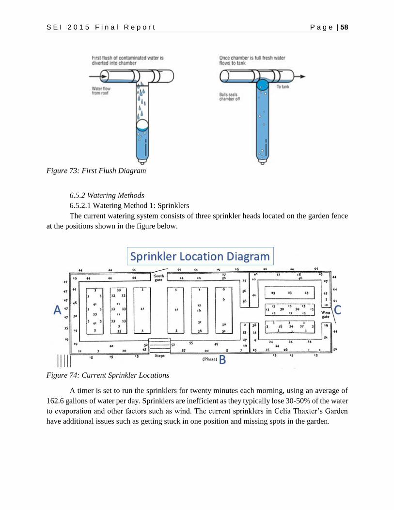
S E I 2 0 1 5 F i n a l R e p o r t P a g e | 58
Figure 73: First Flush Diagram
6.5.2 Watering Methods
6.5.2.1 Watering Method 1: Sprinklers
The current watering system consists of three sprinkler heads located on the garden fence
at the positions shown in the figure below.
Figure 74: Current Sprinkler Locations
A timer is set to run the sprinklers for twenty minutes each morning, using an average of
162.6 gallons of water per day. Sprinklers are inefficient as they typically lose 30-50% of the water
to evaporation and other factors such as wind. The current sprinklers in Celia Thaxter’s Garden
have additional issues such as getting stuck in one position and missing spots in the garden.
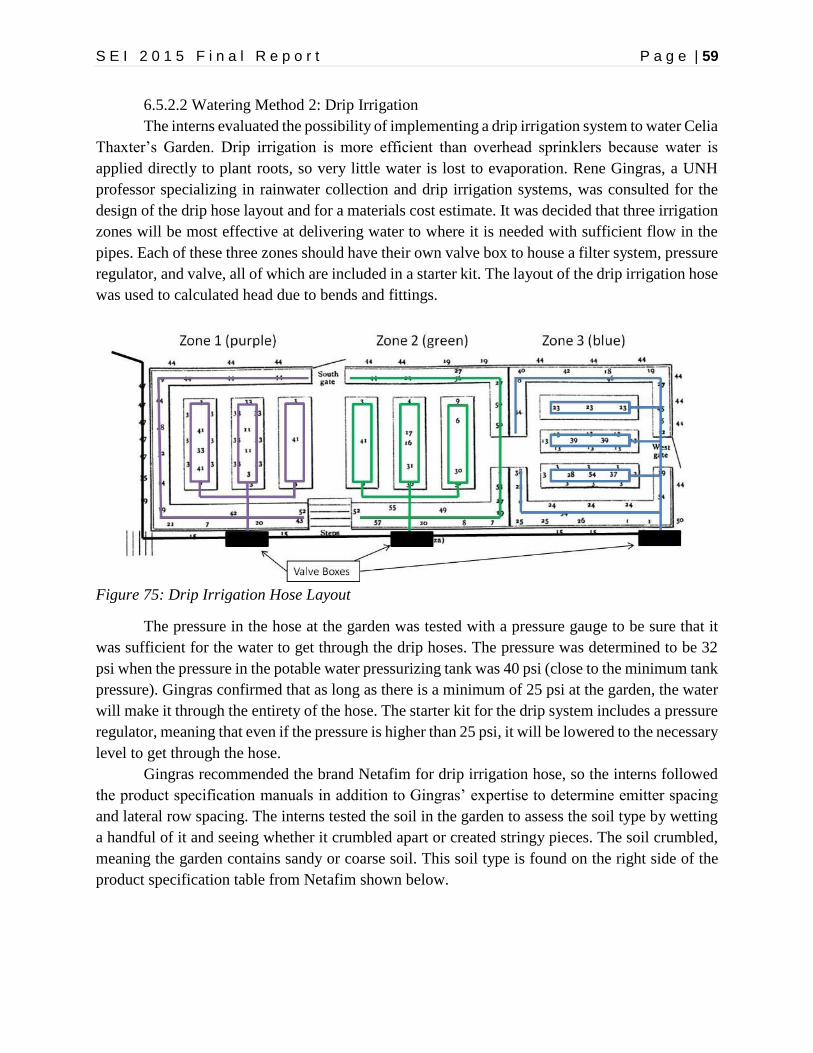
S E I 2 0 1 5 F i n a l R e p o r t P a g e | 59
6.5.2.2 Watering Method 2: Drip Irrigation
The interns evaluated the possibility of implementing a drip irrigation system to water Celia
Thaxter’s Garden. Drip irrigation is more efficient than overhead sprinklers because water is
applied directly to plant roots, so very little water is lost to evaporation. Rene Gingras, a UNH
professor specializing in rainwater collection and drip irrigation systems, was consulted for the
design of the drip hose layout and for a materials cost estimate. It was decided that three irrigation
zones will be most effective at delivering water to where it is needed with sufficient flow in the
pipes. Each of these three zones should have their own valve box to house a filter system, pressure
regulator, and valve, all of which are included in a starter kit. The layout of the drip irrigation hose
was used to calculated head due to bends and fittings.
Figure 75: Drip Irrigation Hose Layout
The pressure in the hose at the garden was tested with a pressure gauge to be sure that it
was sufficient for the water to get through the drip hoses. The pressure was determined to be 32
psi when the pressure in the potable water pressurizing tank was 40 psi (close to the minimum tank
pressure). Gingras confirmed that as long as there is a minimum of 25 psi at the garden, the water
will make it through the entirety of the hose. The starter kit for the drip system includes a pressure
regulator, meaning that even if the pressure is higher than 25 psi, it will be lowered to the necessary
level to get through the hose.
Gingras recommended the brand Netafim for drip irrigation hose, so the interns followed
the product specification manuals in addition to Gingras’ expertise to determine emitter spacing
and lateral row spacing. The interns tested the soil in the garden to assess the soil type by wetting
a handful of it and seeing whether it crumbled apart or created stringy pieces. The soil crumbled,
meaning the garden contains sandy or coarse soil. This soil type is found on the right side of the
product specification table from Netafim shown below.

S E I 2 0 1 5 F i n a l R e p o r t P a g e | 60
Figure 76: Netafim Product Specifications
Based on Gingras’ evaluation of the system needs, an emitter flow of 0.9 gallons per hour
was decided on, as well as emitter spacing of 12 inches and lateral spacing of 12 inches in the
flower beds. It was then determined that the three zones should be put on separate timers so they
will run at different times. Gingras recommended using battery-powered timers so that SML will
not need to run electrical wires up to the valve boxes.
The interns determined the necessary run time for the drip hoses based on the amount of
water currently delivered by the sprinkler system. Taking into account a 30% evaporation rate, the
garden is receiving approximately 112 gallons per day. This equates to 15 cubic feet, which was
then divided by the area of the garden to obtain a value of about 0.25 inches per day as the amount
of water that the garden receives.
In order to provide the garden with 0.25 inches of water per day, the drip hoses should be
run for approximately twenty minutes each, according to the application rates in the Netafim
product specification table above (Figure 34). The longest drip zone includes ninety-six emitters,
which is multiplied by a flow rate of 0.9 gallons per hour for each emitter to give a total flow rate
of 1.44 gpm. This number is taken as a conservative estimate for all three zones, meaning that
watering the three zones for twenty minutes each utilizes 86.4 gallons per day.
A drip irrigation system requires at least 25 psi at the point of discharge. The interns
measured the pressure of one sprinkler at the garden as 32 psi when the tank was at a low pressure
of 40 psi (before the cistern pump turns on). The pressure is adequate for the system and can be
decreased by pressure breakers if needed.
6.5.3 Tank Size Evaluation
Rainfall data from the last five seasons was analyzed to determine average precipitation
patterns. The average number of wet and dry days were four and two, respectively, with an average
precipitation on wet days of 0.3 inches. The total rooftop surface area utilized for rainwater
collection is 2,203 ft2 to provide a total of 411.96 gallons on average for each day of rain. A first
flush system would divert 33.045 gallons in each rainfall event, leaving 395.44 gallons to enter the
collection tanks for each day of rain.

S E I 2 0 1 5 F i n a l R e p o r t P a g e | 61
The two cylindrical collection tanks installed at the beginning of the season are six feet
deep and have a total capacity of 1,600 gallons. The water level should not fall below 0.5 feet so
particles can be allowed to settle at the bottom without getting pumped out. Therefore, the useable
capacity is 1,466.67 gallons.
Models were created to compare the water volume in the tanks for each watering method
over the course of the 100 day season. The tanks were assumed to be full at the start of the season,
with a maximum capacity of 1,466.67 gallons. The models operate on a six day cycle. Water is
removed from the tank to water the garden for four consecutive dry days. The fifth and sixth days
represent a rainfall event. On these days, water is added to the tank by rainfall, and is only removed
from the tank for watering the garden on the fifth day because SML staff manually turn off the
watering system on the sixth day to prevent over-watering.
Figure 77: Fullness of Rainwater Tank With Gutter Filters
Figure 78: Fullness of Rainwater With First Flush
0200400600800
1000120014001600
0 10 20 30 40 50 60 70 80 90 100
Wat
er V
olu
me
(gal
)
Day
Rainwater Tank With Gutter Filters
Sprinklers Drip Irrigation Max Capacity
0
500
1000
1500
2000
0 10 20 30 40 50 60 70 80 90 100Wat
er V
olu
me
(gal
)
Day
Rainwater Tank With First Flush
Sprinklers Drip Irrigation Max Capacity

S E I 2 0 1 5 F i n a l R e p o r t P a g e | 62
Regardless of the filtration system used, the amount of rainwater in the tanks is more than
sufficient for drip irrigation. The lower water usage due to the drip system would ensure that the
tanks are refilled to maximum capacity during each rainfall event. For the sprinkler system, the
tanks would be depleted to a lower volume between rainfall events. With the addition of first flush
to the sprinkler system, the rainfall would not be able to refill the tanks to maximum capacity. This
would result in an overall decline in rainwater volume over the course of the season, but would
still not fully deplete the tanks by the end of the season.
In the case of a dry spell, the current sprinkler system would deplete the tanks in nine days,
assuming they are initially filled to maximum capacity. In contrast, the drip irrigation system
would not deplete the tanks until the seventeenth day without rain.
6.5.4 Pump Calculations and Options
In order to size a pump correctly for the irrigation system, it is important to know the
necessary pump head and water flow rate. The following equation was used to calculate total
pump head for each system:
Equation 12: Head Pump Calculation
● HP = Total pump head
● Δz = Change in elevation
● V = Velocity of water in hose
● g = Gravitational constant
● f = Frictional coefficient
● L = Length of pipe
● D = Diameter of pipe
● kb = Coefficient for pipe bends
● kf = Coefficient for pipe fittings
The interns created a table for the necessary pump head calculation variables for both the
sprinkler system and the drip irrigation system. The head calculated in the column labeled “To
Garden” is added to the head for the two systems because the pump for either irrigation system
still needs to get the water up to the garden in addition to the pump head in the watering system.
The head calculated for the drip irrigation system was used in selecting pumps because drip
irrigation was the recommended option for watering Celia Thaxter’s Garden.

S E I 2 0 1 5 F i n a l R e p o r t P a g e | 63
Table 38: Calculating Head for Sprinkler and Drip Irrigation Systems
To Garden Sprinkler Drip Irrigation
pipe material flex pvc flex pvc polyethelene
delta Z (ft) 11.30 3.50 0.50
V (ft/s) 3.32 5.90 1.88
g (ft/s^2) 32.20 32.20 32.20
f 0.02 0.02 0.02
L (ft) 159.00 72.00 96.00
D (ft) 0.08 0.06 0.05
k bend 4.66 1.98 13.86
k fittings 0.14 0.14 0.14
Hp (ft) 19.31 18.37 3.74
Total Hp (ft) N/A 37.68 23.05
The interns researched pumps that would fit the required head and flow rate of the drip
irrigation system. The head was calculated to be 23.05 feet from the above table, and the flow rate
was found to be 8.13 gpm. This flow rate was determined by taking an average of the readings on
the water flow meter in the generator room over several days. The interns recommend keeping the
same flow rate because the pressure in the hose at the garden is 32 psi, which is a sufficient level
for drip irrigation hoses. Following is a table of pump options that were chosen based on the head
and flow rate specifications.
Table 39: Pump Options
Pump HP Cost GPM
Range
Max
Head
(ft)
Q
(gpm)
at 23 ft
Material Company Pump Type Application
TSC130 1/6 $62.95 13-16 25 5.5 Thermo-
plastic
Wayne Submersible Drain
basements,
boats, sinks
Liberty 1/2 $329.88 0-67 37 35 Cast iron Liberty
Pumps
Submersible High-output
sump
applications
Little
Giant
1/6 $168.00 4-20 26 7 Aluminum Grainger Submersible Sewage/
sump pump
Dayton 1/3 $181.00 0-50 30 17 Cast Iron Grainger Submersible Sump pump

S E I 2 0 1 5 F i n a l R e p o r t P a g e | 64
6.6 Conclusions & Recommendations
6.6.1 Filtration and Watering Method Recommendations
Criteria were chosen for selecting filtration and watering methods and are detailed in the
decision matrices below. Effectiveness was rated as the highest priority because it is most
important that the selected system functions properly. Water collection and use were rated as next
highest to fit with the overarching goal of water conservation. Maintenance and pump size are also
rated at this priority to reduce the amount of work for SML staff and electricity required.
Implementation and cost are rated as the lowest priority because SML has been successful in the
past with having volunteers and receiving grants for sustainable system installations.
Table 40: Comparison of Filtration Methods
Filtration Method Comparison
Priority 2 1 3 2 1
Method Water
Collected Implementation Effectiveness Maintenance Cost Total
Gutter
Filters 412 gal/day
Construct, place
in gutter
Clogs easily,
lets in sand
Wash filters,
clean gutters $0.00
4 Ranking 1 1 0 0 1
First Flush 395 gal/day Adjust gutters,
add flush tank
Removes initial
roof debris
Release flush
tank contents
7 Ranking 1 0 1 1 0
Table 41: Comparison of Watering Methods
Watering Method Comparison
Priority 2 1 3 2 1
Method Water
Use
Implementatio
n Effectiveness
Head/Pump
Size Cost Total
Sprinklers 163
gal/day
Already in
place
Inconsistent,
water
evaporates
38 ft $0.00
2 Ranking 0 1 0 0 1
Drip
Irrigation 86 gal/day
Installation of
drip system
Direct to roots,
steadier flow 23 ft $744
7 Ranking 1 0 1 1 0

S E I 2 0 1 5 F i n a l R e p o r t P a g e | 65
A first flush system in conjunction with drip irrigation is recommended. Both systems were
more effective, which was determined to outweigh their greater costs and implementation.
Additionally, this combination of systems provides cleaner water to the garden and less water is
wasted. While there is adequate flow for both systems, the drip irrigation system is recommended
because a use for the excess rainwater could be found, and then there would be enough water
available for a second use. Also, less energy would be needed to use the drip irrigation system
because it requires a smaller pump. Future research could go into adding soil sensors to the drip
irrigation system so the SML staff do not have to manually shut the watering system off on rainy
days.
Another factor to consider with the first flush is whether debris will fit through the ball
valve. If it is determined that this may be an issue, different types of valves could be researched to
use instead. Gingras mentioned gutter helmets as an additional recommendation for filtering roof
water. Gutter helmets have a specific shape that allows water to flow into the gutter, but debris
falls off the edge. Depending on the cost of gutter helmets, they may be considered as a future
option instead of first flush.
6.6.2 Pump Recommendation
After comparing the pump options from Table 17, the interns recommend that SML get a
Dayton ⅓ hp submersible sump pump. This pump is made of cast iron, which means the pump
will be reliable for several years. Below is the pump curve from the manufacturer.
Figure 79: Pump Curve of Recommended Pump
This pump curve shows that the flow rate at the required head of 23 feet is higher than 8.13
gpm, but this should be fine because the flow can be throttled down if necessary. Combining this
pump with a drip irrigation system will meet the demands of the system and keep Celia Thaxter’s
Garden sufficiently watered with collected rainwater.

S E I 2 0 1 5 F i n a l R e p o r t P a g e | 66
6.7 Resources
"Friction Losses in Pipe Fittings." Web.
<http://www.metropumps.com/ResourcesFrictionLossData.pdf>."Friction Losses in Pipe
Fittings." Web. <http://www.metropumps.com/ResourcesFrictionLossData.pdf>.
Houghtalen, Robert J. "Loss of Head Due to Friction." Fundamentals of Hydraulic Engineering
Systems. By Ned H.C. Hwang. Third ed. New Jersey: Prentice-Hall, 1996. 58-65. Print.
“Moody Diagram.” The Engineering ToolBox. Web.
<http://www.engineeringtoolbox.com/moody-diagram-d_618.html>
"Roughness and Surface Coefficients of Ventilation Ducts." The Engineering ToolBox. Web.
<http://www.engineeringtoolbox.com/surface-roughness-ventilation-ducts-d_209.html>.
"The Texas Manual on Rainwater Collection." The Texas Water Development Board. Web.
<http://www.ecy.wa.gov/programs/wr/hq/pdf/texas_rw_harvestmanual_3rdedition>
“Water - Dynamic and Kinematic Viscosity.” The Engineering ToolBox. Web.
<http://www.engineeringtoolbox.com/water-dynamic-kinematic-viscosity-d_596.html>

S E I 2 0 1 5 F i n a l R e p o r t P a g e | 67
Project 7 - Freshwater Well Siting
7.1 Background
Having an adequate potable freshwater supply is a necessary requirement for drinking,
cleaning, and lab work at SML. This water supply comes from a 20-foot deep freshwater well on
the island. When the water level in the well falls below a certain height, freshwater must be
produced from saltwater through reverse osmosis, an energy intensive and costly process. Previous
interns began examining the hydrology and geology of the existing well’s watershed area.
7.2 Purpose
As freshwater is an essential part of daily life on the island, it is important to make sure the
well is operational and providing a sufficient amount of water. The goal for this project is to
supplement the freshwater well with water in the area that is not being captured. This requires the
interns to quantify the leakage of the existing well to determine if it is worth capturing at another
location within the same watershed. The interns will also study the hydrology and geology of an
SML designated site to determine if it is a suitable place for a new well.
7.3 Scope
The interns calculated the leakage rate from the current well. They also determined if a
new well could be placed in a site chosen by SML staff.
7.4 Methods
7.4.1 Calculating Leakage
Pressure transducers were placed in the existing well to sense the water level over the
winter of 2014-2015. Weather data was collected from Durham, NH for precipitation values. The
interns analyzed this data with the help of Professor Tom Ballestero from UNH. Specific date
ranges were chosen to fit certain conditions in order to calculate the area of the aquifer formation
and leakage at different water depths.
7.4.2 Evaluating New Well Site
The depth of bedrock at the new well site was measured by inserting a length of rebar into
the ground. Test holes were dug in the deepest areas and saturation thickness was measured once
they had filled with water.
7.5 Results & Analysis
7.5.1 Calculating Leakage
The well depth measured in 15 minute intervals and daily rainfall data taken from October
1st, 2014 to May 15th, 2015 are displayed below. Increases in well depth tend to be attributed to
rainfall events that occur in the few days preceding the increase. The spikes in late February and
early March are most likely due to snowmelt, in which the amount of water recharging the well is
dependent on temperature in addition to precipitation.
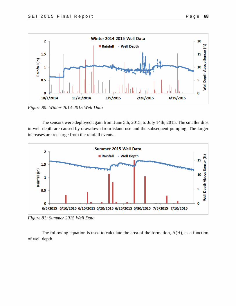
S E I 2 0 1 5 F i n a l R e p o r t P a g e | 68
Figure 80: Winter 2014-2015 Well Data
The sensors were deployed again from June 5th, 2015, to July 14th, 2015. The smaller dips
in well depth are caused by drawdown from island use and the subsequent pumping. The larger
increases are recharge from the rainfall events.
Figure 81: Summer 2015 Well Data
The following equation is used to calculate the area of the formation, A(H), as a function
of well depth.
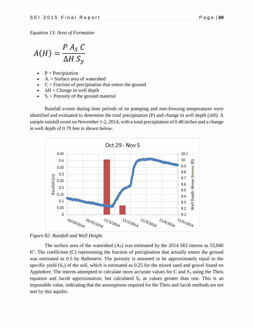
S E I 2 0 1 5 F i n a l R e p o r t P a g e | 69
Equation 13: Area of Formation
P = Precipitation
As = Surface area of watershed
C = Fraction of precipitation that enters the ground
∆H = Change in well depth
Sy = Porosity of the ground material
Rainfall events during time periods of no pumping and non-freezing temperatures were
identified and evaluated to determine the total precipitation (P) and change in well depth (∆H). A
sample rainfall event on November 1-2, 2014, with a total precipitation of 0.48 inches and a change
in well depth of 0.79 feet is shown below.
Figure 82: Rainfall and Well Height
The surface area of the watershed (AS) was estimated by the 2014 SEI interns as 53,840
ft2. The coefficient (C) representing the fraction of precipitation that actually enters the ground
was estimated as 0.5 by Ballestero. The porosity is assumed to be approximately equal to the
specific yield (Sy) of the soil, which is estimated as 0.25 for the mixed sand and gravel found on
Appledore. The interns attempted to calculate more accurate values for C and Sy using the Theis
equation and Jacob approximation, but calculated Sy as values greater than one. This is an
impossible value, indicating that the assumptions required for the Theis and Jacob methods are not
met by this aquifer.

S E I 2 0 1 5 F i n a l R e p o r t P a g e | 70
Using the estimated values, A(H) was calculated for each rainfall event that fit the
necessary criteria. PA(H)C, the total water entering the well when H is the depth of water, was
also calculated. The area was then graphed as a function of well depth after the rainfall event.
Table 42: Effect of Rainfall on Watershed
Start Date End Date Rainfall
(in)
H Before
(ft)
H After
(ft)
Delta H
(ft)
A(H)
(ft2)
PA(H)C
(ft3)
Notes
10/21/2014 10/24/2014 2.43 6.16 9.6 3.44 6338.72 5451.30
11/1/2014 11/2/2014 0.48 9.23 10.02 0.79 5452.15 1076.80
11/6/2014 11/7/2014 0.32 9.79 10.06 0.27 10635.06 717.87
11/17/2014 11/17/2014 0.94 9.59 10.32 0.73 11554.70 2108.73 First frost:
11/19
4/23/2015 4/23/2015 0.07 10.3 10.36 0.06 10468.89 157.03 Pumping:
4/16-4/20
4/28/2015 4/28/2015 0.05 9.94 10.03 0.09 4985.19 112.17 Pumping
began: 5/6
Figure 83: Area with Respect to Height
The following equation uses the area values at depth to calculate the leakage, L(H), of the
formation, also as a function of well depth.
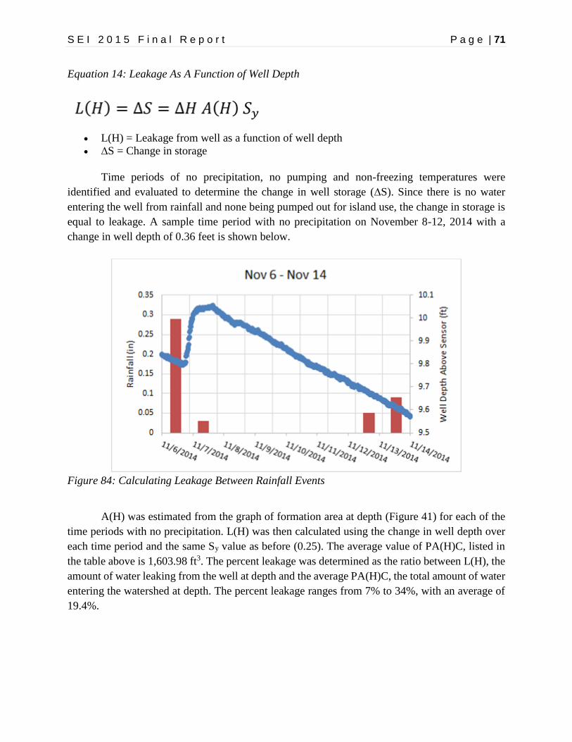
S E I 2 0 1 5 F i n a l R e p o r t P a g e | 71
Equation 14: Leakage As A Function of Well Depth
L(H) = Leakage from well as a function of well depth
∆S = Change in storage
Time periods of no precipitation, no pumping and non-freezing temperatures were
identified and evaluated to determine the change in well storage (∆S). Since there is no water
entering the well from rainfall and none being pumped out for island use, the change in storage is
equal to leakage. A sample time period with no precipitation on November 8-12, 2014 with a
change in well depth of 0.36 feet is shown below.
Figure 84: Calculating Leakage Between Rainfall Events
A(H) was estimated from the graph of formation area at depth (Figure 41) for each of the
time periods with no precipitation. L(H) was then calculated using the change in well depth over
each time period and the same Sy value as before (0.25). The average value of PA(H)C, listed in
the table above is 1,603.98 ft3. The percent leakage was determined as the ratio between L(H), the
amount of water leaking from the well at depth and the average PA(H)C, the total amount of water
entering the watershed at depth. The percent leakage ranges from 7% to 34%, with an average of
19.4%.
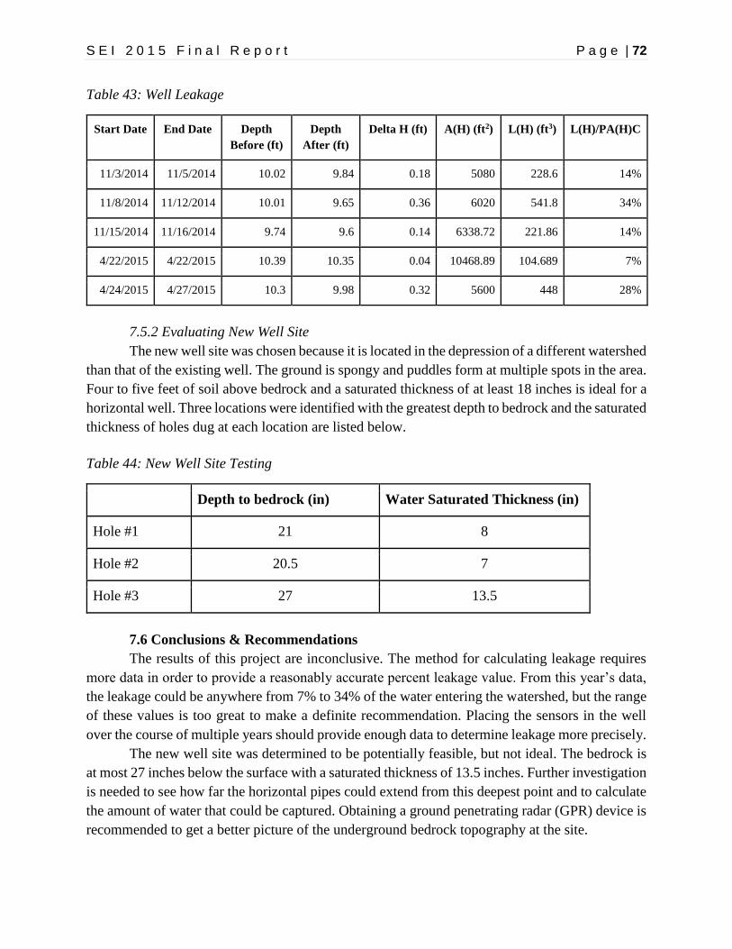
S E I 2 0 1 5 F i n a l R e p o r t P a g e | 72
Table 43: Well Leakage
Start Date End Date Depth
Before (ft)
Depth
After (ft)
Delta H (ft) A(H) (ft2) L(H) (ft3) L(H)/PA(H)C
11/3/2014 11/5/2014 10.02 9.84 0.18 5080 228.6 14%
11/8/2014 11/12/2014 10.01 9.65 0.36 6020 541.8 34%
11/15/2014 11/16/2014 9.74 9.6 0.14 6338.72 221.86 14%
4/22/2015 4/22/2015 10.39 10.35 0.04 10468.89 104.689 7%
4/24/2015 4/27/2015 10.3 9.98 0.32 5600 448 28%
7.5.2 Evaluating New Well Site
The new well site was chosen because it is located in the depression of a different watershed
than that of the existing well. The ground is spongy and puddles form at multiple spots in the area.
Four to five feet of soil above bedrock and a saturated thickness of at least 18 inches is ideal for a
horizontal well. Three locations were identified with the greatest depth to bedrock and the saturated
thickness of holes dug at each location are listed below.
Table 44: New Well Site Testing
Depth to bedrock (in) Water Saturated Thickness (in)
Hole #1 21 8
Hole #2 20.5 7
Hole #3 27 13.5
7.6 Conclusions & Recommendations
The results of this project are inconclusive. The method for calculating leakage requires
more data in order to provide a reasonably accurate percent leakage value. From this year’s data,
the leakage could be anywhere from 7% to 34% of the water entering the watershed, but the range
of these values is too great to make a definite recommendation. Placing the sensors in the well
over the course of multiple years should provide enough data to determine leakage more precisely.
The new well site was determined to be potentially feasible, but not ideal. The bedrock is
at most 27 inches below the surface with a saturated thickness of 13.5 inches. Further investigation
is needed to see how far the horizontal pipes could extend from this deepest point and to calculate
the amount of water that could be captured. Obtaining a ground penetrating radar (GPR) device is
recommended to get a better picture of the underground bedrock topography at the site.

S E I 2 0 1 5 F i n a l R e p o r t P a g e | 73
If there is significant leakage from the existing well, it would be worthwhile to investigate
the feasibility of capturing the water at a point downgradient of the existing well within the same
watershed. Otherwise, a new well site in a different watershed is more likely to yield more water
for supplementation of the current system. Potential new well sites should be identified and tested
according to the methods outlined above to determine the bedrock depth and saturation thickness.
These sites can then be evaluated in addition to the potential site from this study in order to
determine the most promising course of action.
7.7 References
"Soil & Aquifer Properties That Affect Groundwater." Web.
<http://www.co.portage.wi.us/groundwater/undrstnd/soil.htm>.

S E I 2 0 1 5 F i n a l R e p o r t P a g e | 74
Future Project Recommendations
Correcting and Updating GIS Map
A map of Appledore’s system is necessary for SML staff and interns to determine where
exactly a system is running (electrical wires, pipes, etc.). An application that easily displays this is
GIS. There is currently an SML GIS page, but it has some mistakes and things left out. Updating
the system will help SML staff and future interns know where the systems are running on the island
for future maintenance and projects.
Well Site to Capture Leakage from Current Well
Continue analyzing the data from the well meters to determine what the leakage percentage
is for the current well’s watershed. If the percentage of leakage is high, look for an area within the
same watershed for a new well.
Well Site Next to Crystal Lake to Capture Spring Water
Examine potential well site near Crystal Lake. Examine groundwater quality nearby and
whether there is a location with enough soil above the bedrock to dig a well.
Bird Deterrents to Increase Solar Panel Efficiency
Brainstorm and implement devices to deter birds from sitting on top of solar panels.
Measure whether there is an increase in efficiency to determine which device works best in terms
of efficiency and least harmful to gulls.
Look at Electrical Load Compared to the Number and Type of People on Island
Record the total island energy used each 24 hour period, including the Energy Conservation
Building Grid and the Green Grid. Record the number of overnight residents, day visitors, and
types of people on the island over the same period of time, so that a comparison between energy
use and people on island can be made.

S E I 2 0 1 5 F i n a l R e p o r t P a g e | 75
Acknowledgements
Thank you to all of the SML staff and mentors that have helped us during our time here at
Appledore. We appreciate all of the time, energy, guidance, and chocolate that you have
provided us with.
Ross Hansen
Mike Rosen
Tom Johnson
Mike Dalton
Nancy Kinner
Alex Brickett
Dylan Whitney
Alexa Hilmer
John Durant
Lee Consavage
Tom Ballestero
Justin Eisfeller
Andrew Jacobs
Rene Gingras

S E I 2 0 1 5 F i n a l R e p o r t P a g e | 76
Appendix
Project 1 – LED Lighting Study
LED Recommended Light Levels
Illuminance (lux) Space
50 Dark public spaces
100 Corridors, loading bays
150 Warehouses, theaters
200 Foyers, homes, bathrooms
300 Classrooms, assembly halls
400 Offices, libraries, kitchens
500 Computers, labs, stores
750 Workshops, supermarkets
1000 Detailed workspaces
Cost analysis calculations were performed following this sample calculation for Kiggins Kitchen,
which currently has 46 fluorescent T-8 bulbs. The total wattage includes both the bulb (32 W) and
the ballast (53 W) for each pair of bulbs. Since the LED bulbs do not require ballasts, the total
wattage is the same as the bulb wattage (17.2 W).
𝑊𝑎𝑡𝑡𝑎𝑔𝑒 (𝐹𝑙𝑢𝑜𝑟𝑒𝑠𝑐𝑒𝑛𝑡) = 𝐵𝑢𝑙𝑏 + 𝐵𝑎𝑙𝑙𝑎𝑠𝑡 = 32 𝑊 + 53 𝑊
2 𝑏𝑢𝑙𝑏𝑠 = 58.5 𝑊
It was estimated that the kitchen lights are on for 18 hours each day of a 100 day season.
𝐴𝑛𝑛𝑢𝑎𝑙 𝑈𝑠𝑎𝑔𝑒 = 18 ℎ
𝑑𝑎𝑦 ∗ 100
𝑑𝑎𝑦
𝑠𝑒𝑎𝑠𝑜𝑛 = 1800
ℎ
𝑠𝑒𝑎𝑠𝑜𝑛
The energy usage and cost can be calculated using $0.54/kWh as the cost of electricity.
𝐴𝑛𝑛𝑢𝑎𝑙 𝐸𝑛𝑒𝑟𝑔𝑦 (𝐹𝑙𝑢𝑜𝑟𝑒𝑠𝑐𝑒𝑛𝑡) = # 𝐵𝑢𝑙𝑏𝑠 ∗ 𝑊𝑎𝑡𝑡𝑎𝑔𝑒 ∗ 𝐴𝑛𝑛𝑢𝑎𝑙 𝑈𝑠𝑎𝑔𝑒
= 46 ∗ 58.5 𝑊 ∗ 1800 ℎ
𝑠𝑒𝑎𝑠𝑜𝑛 = 4843800
𝑊ℎ
𝑠𝑒𝑎𝑠𝑜𝑛 = 4843.8
𝑘𝑊ℎ
𝑠𝑒𝑎𝑠𝑜𝑛
𝐸𝑛𝑒𝑟𝑔𝑦 𝐶𝑜𝑠𝑡 (𝐹𝑙𝑢𝑜𝑟𝑒𝑠𝑐𝑒𝑛𝑡) = 𝐴𝑛𝑛𝑢𝑎𝑙 𝐸𝑛𝑒𝑟𝑔𝑦 ∗ 𝐸𝑙𝑒𝑐𝑡𝑟𝑖𝑐𝑖𝑡𝑦 𝐶𝑜𝑠𝑡
= 4843.8 𝑘𝑊ℎ
𝑠𝑒𝑎𝑠𝑜𝑛 ∗
$0.54
𝑘𝑊ℎ =
$2615.65
𝑠𝑒𝑎𝑠𝑜𝑛

S E I 2 0 1 5 F i n a l R e p o r t P a g e | 77
𝐴𝑛𝑛𝑢𝑎𝑙 𝐸𝑛𝑒𝑟𝑔𝑦 (𝐿𝐸𝐷) = # 𝐵𝑢𝑙𝑏𝑠 ∗ 𝑊𝑎𝑡𝑡𝑎𝑔𝑒 ∗ 𝐴𝑛𝑛𝑢𝑎𝑙 𝑈𝑠𝑎𝑔𝑒
= 46 ∗ 17.2 𝑊 ∗ 1800 ℎ
𝑠𝑒𝑎𝑠𝑜𝑛 = 1424160
𝑊ℎ
𝑠𝑒𝑎𝑠𝑜𝑛 = 1424.16
𝑘𝑊ℎ
𝑠𝑒𝑎𝑠𝑜𝑛
𝐸𝑛𝑒𝑟𝑔𝑦 𝐶𝑜𝑠𝑡 (𝐿𝐸𝐷) = 𝐴𝑛𝑛𝑢𝑎𝑙 𝐸𝑛𝑒𝑟𝑔𝑦 ∗ 𝐸𝑙𝑒𝑐𝑡𝑟𝑖𝑐𝑖𝑡𝑦 𝐶𝑜𝑠𝑡
= 1424.16𝑘𝑊ℎ
𝑠𝑒𝑎𝑠𝑜𝑛 ∗
$0.54
𝑘𝑊ℎ =
$769.05
𝑠𝑒𝑎𝑠𝑜𝑛
The cost of replacing the bulbs can be calculated using $2.00 as the price of each new fluorescent
bulb that lasts for 10,000 hours and $30.00 as the price of each new LED bulb that lasts for 50,000
hours.
𝑅𝑒𝑝𝑙𝑎𝑐𝑒𝑚𝑒𝑛𝑡 𝐶𝑜𝑠𝑡 (𝐹𝑙𝑢𝑜𝑟𝑒𝑠𝑐𝑒𝑛𝑡) = # 𝐵𝑢𝑙𝑏𝑠 ∗ 𝑃𝑟𝑖𝑐𝑒
10000 ℎ∗ 𝐴𝑛𝑛𝑢𝑎𝑙 𝑈𝑠𝑎𝑔𝑒
= 46 ∗ $2.00
10000 ℎ∗ 1800
ℎ
𝑠𝑒𝑎𝑠𝑜𝑛 =
$16.56
𝑠𝑒𝑎𝑠𝑜𝑛
𝑅𝑒𝑝𝑙𝑎𝑐𝑒𝑚𝑒𝑛𝑡 𝐶𝑜𝑠𝑡 (𝐿𝐸𝐷) = # 𝐵𝑢𝑙𝑏𝑠 ∗ 𝑃𝑟𝑖𝑐𝑒
10000 ℎ∗ 𝐴𝑛𝑛𝑢𝑎𝑙 𝑈𝑠𝑎𝑔𝑒
= 46 ∗ $30.00
50000 ℎ∗ 1800
ℎ
𝑠𝑒𝑎𝑠𝑜𝑛 =
$49.68
𝑠𝑒𝑎𝑠𝑜𝑛
The total annual cost of the current bulbs in the kitchen is the sum of energy and replacement costs.
𝐴𝑛𝑛𝑢𝑎𝑙 𝐶𝑜𝑠𝑡 (𝐹𝑙𝑢𝑜𝑟𝑒𝑠𝑐𝑒𝑛𝑡) = 𝐸𝑛𝑒𝑟𝑔𝑦 𝐶𝑜𝑠𝑡 + 𝑅𝑒𝑝𝑙𝑎𝑐𝑒𝑚𝑒𝑛𝑡 𝐶𝑜𝑠𝑡
= $2615.65
𝑠𝑒𝑎𝑠𝑜𝑛 +
$16.56
𝑠𝑒𝑎𝑠𝑜𝑛 =
$2632.21
𝑠𝑒𝑎𝑠𝑜𝑛
𝐴𝑛𝑛𝑢𝑎𝑙 𝐶𝑜𝑠𝑡 (𝐿𝐸𝐷) = 𝐸𝑛𝑒𝑟𝑔𝑦 𝐶𝑜𝑠𝑡 + 𝑅𝑒𝑝𝑙𝑎𝑐𝑒𝑚𝑒𝑛𝑡 𝐶𝑜𝑠𝑡
= $796.05
𝑠𝑒𝑎𝑠𝑜𝑛 +
$49.68
𝑠𝑒𝑎𝑠𝑜𝑛 =
$818.73
𝑠𝑒𝑎𝑠𝑜𝑛
The energy and cost savings of installing LEDs are the difference between the current fluorescent
and proposed LED values.
𝐴𝑛𝑛𝑢𝑎𝑙 𝐸𝑛𝑒𝑟𝑔𝑦 𝑆𝑎𝑣𝑖𝑛𝑔𝑠 = 𝐴𝑛𝑛𝑢𝑎𝑙 𝐸𝑛𝑒𝑟𝑔𝑦 (𝐹𝑙𝑢𝑜𝑟𝑒𝑠𝑐𝑒𝑛𝑡) − 𝐴𝑛𝑛𝑢𝑎𝑙 𝐸𝑛𝑒𝑟𝑔𝑦 (𝐿𝐸𝐷)
= 4843.8 𝑘𝑊ℎ
𝑠𝑒𝑎𝑠𝑜𝑛 − 1424.16
𝑘𝑊ℎ
𝑠𝑒𝑎𝑠𝑜𝑛 = 3419.64
𝑘𝑊ℎ
𝑠𝑒𝑎𝑠𝑜𝑛
𝐴𝑛𝑛𝑢𝑎𝑙 𝐶𝑜𝑠𝑡 𝑆𝑎𝑣𝑖𝑛𝑔𝑠 = 𝐴𝑛𝑛𝑢𝑎𝑙 𝐶𝑜𝑠𝑡 (𝐹𝑙𝑢𝑜𝑟𝑒𝑠𝑐𝑒𝑛𝑡) − 𝐴𝑛𝑛𝑢𝑎𝑙 𝐶𝑜𝑠𝑡 (𝐿𝐸𝐷)
= $2632.21
𝑠𝑒𝑎𝑠𝑜𝑛 −
$818.73
𝑠𝑒𝑎𝑠𝑜𝑛 =
$1813.49
𝑠𝑒𝑎𝑠𝑜𝑛

S E I 2 0 1 5 F i n a l R e p o r t P a g e | 78
The total cost of installing LEDs can be used to calculate the payback of the project.
𝐼𝑚𝑝𝑙𝑒𝑚𝑒𝑛𝑡𝑎𝑡𝑖𝑜𝑛 𝐶𝑜𝑠𝑡 = # 𝐵𝑢𝑙𝑏𝑠 ∗ 𝑃𝑟𝑖𝑐𝑒 = 46 ∗ $30.00 = $1380
𝑃𝑎𝑦𝑏𝑎𝑐𝑘 = 𝐼𝑚𝑝𝑙𝑒𝑚𝑒𝑛𝑡𝑎𝑡𝑖𝑜𝑛 𝐶𝑜𝑠𝑡
𝐴𝑛𝑛𝑢𝑎𝑙 𝐶𝑜𝑠𝑡 𝑆𝑎𝑣𝑖𝑛𝑔𝑠 =
$1380
$ 1813.49/𝑦𝑒𝑎𝑟 = 0.76 𝑦𝑒𝑎𝑟𝑠
The total diesel fuel savings were calculated according to the data from 2014. The total power
generated was 26.176 MWh and the total amount consumed was 2,342 gallons.
𝐷𝑖𝑒𝑠𝑒𝑙 𝐸𝑛𝑒𝑟𝑔𝑦 = 𝑃𝑜𝑤𝑒𝑟 𝐺𝑒𝑛𝑒𝑟𝑎𝑡𝑒𝑑
𝐷𝑖𝑒𝑠𝑒𝑙 𝐶𝑜𝑛𝑠𝑢𝑚𝑒𝑑=
26.176 𝑀𝑊ℎ
2342 𝑔𝑎𝑙=
11180 𝑀𝑊ℎ
𝑔𝑎𝑙 = 11.18
𝑘𝑊ℎ
𝑔𝑎𝑙
𝐷𝑖𝑒𝑠𝑒𝑙 𝑆𝑎𝑣𝑖𝑛𝑔𝑠 = 𝐴𝑛𝑛𝑢𝑎𝑙 𝐸𝑛𝑒𝑟𝑔𝑦 𝑆𝑎𝑣𝑖𝑛𝑔𝑠
𝐷𝑖𝑒𝑠𝑒𝑙 𝐸𝑛𝑒𝑟𝑔𝑦=
3419.64 𝑘𝑊ℎ/𝑠𝑒𝑎𝑠𝑜𝑛
11.18 𝑘𝑊ℎ/𝑔𝑎𝑙= 305.87
𝑔𝑎𝑙
𝑠𝑒𝑎𝑠𝑜𝑛
Project 2 - ECB Performance / Dashboard
The raw difference between fluke meter and battery monitor data was calculated for each time
interval and averaged for each trial.
𝑅𝑎𝑤 𝐷𝑖𝑓𝑓𝑒𝑟𝑒𝑛𝑐𝑒 = 𝐹𝑙𝑢𝑘𝑒 𝑀𝑒𝑡𝑒𝑟 − 𝐵𝑎𝑡𝑡𝑒𝑟𝑦 𝑀𝑜𝑛𝑖𝑡𝑜𝑟
The average differences were sorted in order. Below are the sorted average differences for trial 1
of current.
-21.11 -5.68 -5.47 -2.66 -2.48 -1.01 0.06 1.18 5.74 10.05
The 1st Quartile is -5.47 and the 3rd Quartile is 1.18. The Interquartile Range (IQR) is the
difference between these values.
𝐼𝑄𝑅 = 3𝑟𝑑 𝑄𝑢𝑎𝑟𝑡𝑖𝑙𝑒 − 1𝑠𝑡 𝑄𝑢𝑎𝑟𝑡𝑖𝑙𝑒 = 1.18 − (−5.47) = 6.66
The range for outliers is then:
𝑂𝑢𝑡𝑙𝑖𝑒𝑟𝑠 < 1𝑠𝑡 𝑄𝑢𝑎𝑟𝑡𝑖𝑙𝑒 − 1.5 ∗ 𝐼𝑄𝑅 = −5.47 − 1.5 ∗ 6.66 = −15.46
𝑂𝑢𝑡𝑙𝑖𝑒𝑟𝑠 > 3𝑟𝑑 𝑄𝑢𝑎𝑟𝑡𝑖𝑙𝑒 + 1.5 ∗ 𝐼𝑄𝑅 = 1.18 + 1.5 ∗ 6.66 = 11.17
The value -21.11 is less than the lower bound of -15.46 and is therefore an outlier. This value is
for Battery Bank 2.

S E I 2 0 1 5 F i n a l R e p o r t P a g e | 79
Project 3 - Saltwater Pump Efficiency
Eagle 440 Electrical Load Profile Saltwater Pump

S E I 2 0 1 5 F i n a l R e p o r t P a g e | 80
Atmospheric pressure at sea level = Ha
Change in elevation = Hz
Flow = Q; a range of gpm from 0 to 60
Cross sectional area of intake pipe = A
Diameter of intake pipe = Dintake
Friction head loss = Hf
Vapor pressure of seawater = Hvp
System Curve Equations

S E I 2 0 1 5 F i n a l R e p o r t P a g e | 81
Recommended Grundfos Pump Distributors:
1. DL Thurrot Inc
Address: 84 Eastern Ave, Waterville, ME 04901
Phone: (207) 873-0860
2. Atlantic Pump & Engineering
Address: 51 Eagle Dr, Sanford, ME 04073
Phone: (207) 324-2405
Project 4 - Electrical Transformer Study
Line Losses if Transformers Removed
*All wire gauge size is 1/0, Effective Z from table is 0.13.
*Bartels includes line losses from ECB to Kiggins at 480V
*Laighton and K-House include line losses from ECB to Kiggins to Tower at 480V
Cable
Length
(ft)
Actual
Effective
Z
HV
Current
(A)
Voltage
to
Power
(W)
LV
Current
(A)
Voltage
Drop
(V)
Line
Loss at
Total
Power

S E I 2 0 1 5 F i n a l R e p o r t P a g e | 82
Neutral
(V)
208V
(kW)
Loss
(kW)
Bartels 450 0.117 36 277 9972 83.1 9.72 0.8080 1.44
Laighton 140 0.0364 36 277 9972 83.1 3.02 0.2514 1.04
K-House 378 0.09828 36 277 9972 83.1 8.17 0.6787 1.47
Project 5 - Electrical Load Profiles
Eagle 440 Electrical Load Profile Kiggins

S E I 2 0 1 5 F i n a l R e p o r t P a g e | 83
Eagle 440 Electrical Load Profile Refrigeration

S E I 2 0 1 5 F i n a l R e p o r t P a g e | 84
Eagle 440 Power Data for Each Building & Large Appliance
Building/
Appliance
Net Power
(kVAh) Time (hours) Power (kVA)
Estimated Power Each Day
(kVAh/24 Hours)
Bartels 3.47 23.37 0.148 3.564
Kiggins 268.44 41.78 6.425 154.202
ECB 570.68 24.68 23.123 554.956
Laighton 18.53 21.33 0.869 20.850
K-House 7.12 30.98 0.230 5.515
Refrigeration 22.358 68.75 0.325 7.805
Freezer 8.477 23.4 0.362 8.694
Saltwater
Pump 53.47 15.5 3.450 82.792
Pie Chart Data
Building
Total
Wattage
Wattage
Percentage
Load
(kWh/yr)
Load
(kWh/day)
Load
Percentage
Grass Lab 15,768.0 18.48 5860 49 12.7
Dive Shack 11,000.0 12.89 132 1 0.3
Founders 1,105.0 1.29 290 2 0.6
Kiggins Commons 39,253.0 46 26036 217 56.3
Laighton 2,743.0 3.21 1896 16 4.1
Hamilton 1,439.0 1.69 113 1 0.2
Palmer-Kinne Lab 3,448.0 4.04 2556 21 5.5
Kingsbury House 5,650.0 6.62 3447 29 7.5
Bartels 4,930.0 5.78 5958 50 12.9
Total 85,336.0 100 46288 385.73 100.0
Project 6 – Rainwater Collection for Celia Thaxter’s Garden
There are two 800 gallon rainwater collection tanks located behind the Utility Building. The tanks
are 6 feet in height but the water level should not be allowed to drop below 6 inches. The useable
volume of rainfall can then be calculated as:
𝑈𝑠𝑒𝑎𝑏𝑙𝑒 𝑅𝑎𝑖𝑛𝑤𝑎𝑡𝑒𝑟 = 1600 𝑔𝑎𝑙 ∗5.5 𝑓𝑡
6 𝑓𝑡= 14.66.67𝑔𝑎𝑙

S E I 2 0 1 5 F i n a l R e p o r t P a g e | 85
The water demand for each watering method can be calculated with flow rate (Q) and run time (t).
The sprinkler system runs for 20 minutes each morning with an average flow rate of 8.13 gallons
per minute.
𝑆𝑝𝑟𝑖𝑛𝑘𝑙𝑒𝑟 𝑊𝑎𝑡𝑒𝑟 𝐷𝑒𝑚𝑎𝑛𝑑 = 𝑄 ∗ 𝑡 = 8.13 𝑔𝑎𝑙
𝑚𝑖𝑛∗ 20 𝑚𝑖𝑛 = 162.6 𝑔𝑎𝑙
The drip hoses should provide an equivalent amount of water as the current system. This amount
can be determined using a 30% evaporation rate from the sprinklers and the area of the garden (15
by 50 feet).
𝐷𝑎𝑖𝑙𝑦 𝑊𝑎𝑡𝑒𝑟 𝐷𝑒𝑚𝑎𝑛𝑑 =0.7𝑄
𝐴=
0.7 ∗ 162.6 𝑔𝑎𝑙 ∗1
7.48𝑓𝑡3
𝑔𝑎𝑙
750 𝑓𝑡2= 0.02 𝑓𝑡3 = 0.24 𝑖𝑛
The drip hose recommends 20 minutes of watering for each ¼ inch of water. The drip irrigation
system would have therefore have three zones that are watered for 20 minutes each. The 0.9 gallon
per hour emitters are spaced 1 foot apart along a 96 foot hose for the longest zone.
𝐷𝑟𝑖𝑝 𝐼𝑟𝑟𝑖𝑔 𝑊𝑎𝑡𝑒𝑟 𝐷𝑒𝑚𝑎𝑛𝑑 = 𝑄 ∗ 𝑡 = 96 𝑓𝑡 ∗ 0.9 𝑔𝑎𝑙
𝑓𝑡 ℎ𝑟∗
1 ℎ𝑟
60 𝑚𝑖𝑛∗ 20 𝑚𝑖𝑛 ∗ 3 = 86.4 𝑔𝑎𝑙
The volume of rainfall for each day of a rainstorm is dependent on the average rainfall per day (0.3
inches) and surface area of the roof (2203 ft2).
𝑅𝑎𝑖𝑛 𝑉𝑜𝑙𝑢𝑚𝑒 = 𝐴𝑣𝑔 𝑅𝑎𝑖𝑛 ∗ 𝑅𝑜𝑜𝑓 𝐴𝑟𝑒𝑎 = 0.3 𝑖𝑛
𝑑𝑎𝑦∗
1 𝑓𝑡
12 𝑖𝑛∗ 2203 𝑓𝑡2 = 411.96
𝑔𝑎𝑙
𝑑𝑎𝑦
A first flush system should divert 1-2 gallons of rainwater for every 100 ft2 of roof area. An average
of 1.5 gallons was determined to be sufficient. The total volume of water diverted for each
rainstorm can be calculated as:
𝑊𝑎𝑡𝑒𝑟 𝐷𝑖𝑣𝑒𝑟𝑡𝑒𝑑 = 1.5 𝑔𝑎𝑙
100 𝑓𝑡2∗ 2203 𝑓𝑡2 = 33.05 𝑔𝑎𝑙
Using an average 2 day rainstorm, the volume of rainfall added to the system with first flush for
each day of a rainstorm would then be calculated as:
𝑅𝑎𝑖𝑛 𝑉𝑜𝑙𝑢𝑚𝑒 (𝐹𝑖𝑟𝑠𝑡 𝐹𝑙𝑢𝑠ℎ) = 411.96 𝑔𝑎𝑙
𝑑𝑎𝑦−
33.05 𝑔𝑎𝑙
2 𝑑𝑎𝑦𝑠= 395.44
𝑔𝑎𝑙
𝑑𝑎𝑦

S E I 2 0 1 5 F i n a l R e p o r t P a g e | 86
The following equation was used to calculate total pump head (HP) for each system, where Δz is
change in elevation, V is velocity, g is the gravitational constant, f is the frictional coefficient, L
is length of pipe, D is diameter of pipe, kb is the coefficient for bends, and kf is the coefficient for
fittings.
𝐻𝑃 = ∆𝑧 +𝑉2
2𝑔(
𝑓𝐿
𝐷+ 𝑘𝑏 + 𝑘𝑓)
For the current system, the 1 inch diameter pipe travels a total of 159 feet from the collection tanks,
up the side of the Utility Building, and across the grass to the garden. The change in elevation from
inside the tank to the top of the Utility Building is 11.3 feet.
The velocity is determined by the flow rate (Q) and cross section area (A) of the pipe. The average
flow rate in the pipe up to garden in the current system is 8.13 gpm.
𝑉 =𝑄
𝐴=
𝑄𝜋4 𝑑2
=8.13
𝑔𝑎𝑙𝑚𝑖𝑛 ∗
17.48
𝑓𝑡3
𝑔𝑎𝑙∗
160
𝑚𝑖𝑛𝑠𝑒𝑐
𝜋4 (
1 12 𝑓𝑡)
2 = 3.32 𝑓𝑡
𝑠𝑒𝑐
The pipe material is flexible PVC and will have to pass through six 90 bends, two 45 degree
bends, and two valves. The Moody diagram shown below was used to determine the frictional
coefficient (f). The relative roughness is the ratio between absolute roughness (k) and pipe
diameter (D). Reynolds number (NR) is determined by pipe diameter (D), velocity (V), and
kinematic viscosity (ν). The absolute roughness for flexible PVC is 1.4x10⁻⁵ feet and the kinematic
viscosity of 18.4C water is 1.1x10⁻⁵ ft2/sec.
𝑘
𝐷=
1.4 𝑥 10−5 𝑓𝑡
112 𝑓𝑡
= 1.68 𝑥 10−4
𝑁𝑅 =𝐷𝑉
𝜈=
112 𝑓𝑡 ∗ 3.32
𝑓𝑡𝑠𝑒𝑐
1.1 𝑥 10−5 𝑓𝑡2
𝑠𝑒𝑐
= 2.52 𝑥 104
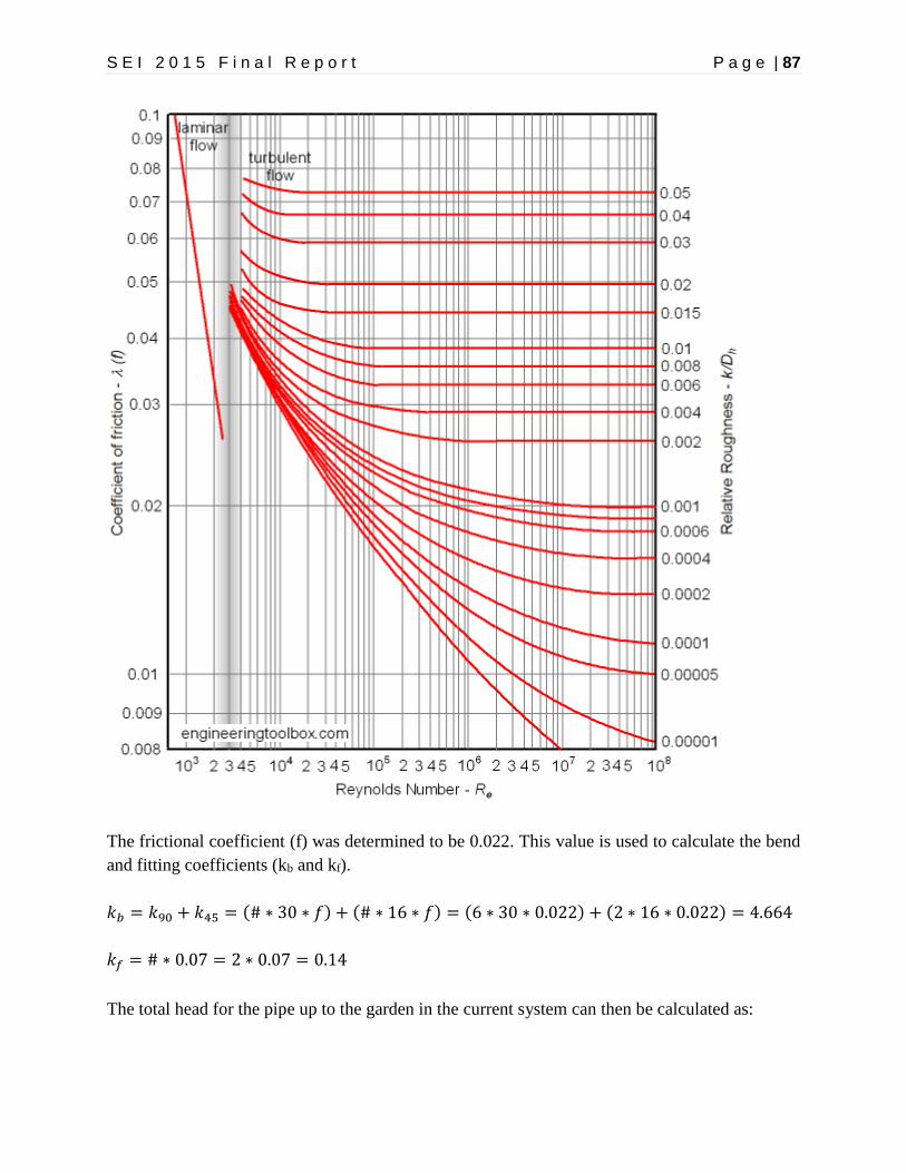
S E I 2 0 1 5 F i n a l R e p o r t P a g e | 87
The frictional coefficient (f) was determined to be 0.022. This value is used to calculate the bend
and fitting coefficients (kb and kf).
𝑘𝑏 = 𝑘90 + 𝑘45 = (# ∗ 30 ∗ 𝑓) + (# ∗ 16 ∗ 𝑓) = (6 ∗ 30 ∗ 0.022) + (2 ∗ 16 ∗ 0.022) = 4.664
𝑘𝑓 = # ∗ 0.07 = 2 ∗ 0.07 = 0.14
The total head for the pipe up to the garden in the current system can then be calculated as:

S E I 2 0 1 5 F i n a l R e p o r t P a g e | 88
𝐻𝑃 (𝑇𝑜 𝐺𝑎𝑟𝑑𝑒𝑛) = 11.3 𝑓𝑡 +(3.32
𝑓𝑡𝑠𝑒𝑐)
2
2 (32.2 𝑓𝑡
𝑠𝑒𝑐2)(
0.022(159 𝑓𝑡)
112 𝑓𝑡
+ 4.664 + 0.14) = 19.31 𝑓𝑡
Additional head calculations need to be made for the separate sections of sprinkler and drip
irrigation systems after the pipe reaches the garden. The sprinklers are attached to the garden fence
3.5 feet above the ground. The longest length of pipe (to the third sprinkler) is 72 feet with a
diameter of 0.75 inches. The flow rate is the same as in the pipe up to the garden, 8.13 gpm.
𝑉 =𝑄
𝐴=
𝑄𝜋4 𝑑2
=8.13
𝑔𝑎𝑙𝑚𝑖𝑛 ∗
17.48
𝑓𝑡3
𝑔𝑎𝑙∗
160
𝑚𝑖𝑛𝑠𝑒𝑐
𝜋4 (
0.7512 𝑓𝑡)
2 = 5.90 𝑓𝑡
𝑠𝑒𝑐
The frictional coefficient (f) is the same as before, 0.022. There are three 90 bends and two valves.
𝑘𝑏 = 𝑘90 = (# ∗ 30 ∗ 𝑓) = (3 ∗ 30 ∗ 0.022) = 1.98
𝑘𝑓 = # ∗ 0.07 = 2 ∗ 0.07 = 0.14
The head for the sprinklers alone is added to the head of the pipe up to the garden to get total head
for the current system.
𝐻𝑃 (𝑆𝑝𝑟𝑖𝑛𝑘𝑙𝑒𝑟) = 3.5 𝑓𝑡 +(5.90
𝑓𝑡𝑠𝑒𝑐)
2
2 (32.2 𝑓𝑡
𝑠𝑒𝑐2)(
0.022(72 𝑓𝑡)
0.7512 𝑓𝑡
+ 1.98 + 0.14) = 18.37 𝑓𝑡
𝐻𝑃 (𝐶𝑢𝑟𝑟𝑒𝑛𝑡) = 𝐻𝑃 (𝑇𝑜 𝐺𝑎𝑟𝑑𝑒𝑛) + 𝐻𝑃 (𝑆𝑝𝑟𝑖𝑛𝑘𝑙𝑒𝑟) = 19.31 𝑓𝑡 + 18.37 𝑓𝑡 = 37.68 𝑓𝑡
For the drip irrigation system, the change in elevation within the garden is 0.5 feet. The longest
length of hose is 96 feet with a diameter of 0.56 inches. The flow rate is 86.4 gph or 1.44 gpm.
𝑉 =𝑄
𝐴=
𝑄𝜋4 𝑑2
=1.44
𝑔𝑎𝑙𝑚𝑖𝑛 ∗
17.48
𝑓𝑡3
𝑔𝑎𝑙∗
160
𝑚𝑖𝑛𝑠𝑒𝑐
𝜋4 (
0.5612 𝑓𝑡)
2 = 1.88 𝑓𝑡
𝑠𝑒𝑐
The frictional coefficient remains the same and the system has twenty-one 90 bends and two
valves.

S E I 2 0 1 5 F i n a l R e p o r t P a g e | 89
𝑘𝑏 = 𝑘90 = (# ∗ 30 ∗ 𝑓) = (21 ∗ 30 ∗ 0.022) = 13.86
𝑘𝑓 = # ∗ 0.07 = 2 ∗ 0.07 = 0.14
The head for the drip hoses is added to the head of the pipe up to the garden to get total head for
the drip irrigation system.
𝐻𝑃 (𝐷𝑟𝑖𝑝 𝐻𝑜𝑠𝑒𝑠) = 0.5 𝑓𝑡 +(1.88
𝑓𝑡𝑠𝑒𝑐)
2
2 (32.2 𝑓𝑡
𝑠𝑒𝑐2)(
0.022(96 𝑓𝑡)
0.5612 𝑓𝑡
+ 13.86 + 0.14) = 3.74 𝑓𝑡
𝐻𝑃 (𝐶𝑢𝑟𝑟𝑒𝑛𝑡) = 𝐻𝑃 (𝑇𝑜 𝐺𝑎𝑟𝑑𝑒𝑛) + 𝐻𝑃 (𝑆𝑝𝑟𝑖𝑛𝑘𝑙𝑒𝑟) = 19.31 𝑓𝑡 + 3.74 𝑓𝑡 = 23.05 𝑓𝑡
Project 7 – Freshwater Well Siting
For the rainfall event on November 1-2, 2014, the total precipitation (P) was 0.48 inches and
changed the well depth (ΔH) by 0.79 feet. AS is 53,840 ft2 from a previous SEI report. C and Sy
are estimated as 0.5 and 0.25, respectively. The area of the formation, A(H), and total amount of
water entering the watershed, PA(H)C, are calculated as:
𝐴(𝐻) =𝑃 𝐴𝑆 𝐶
∆𝐻 𝑆𝑦=
0.48 𝑖𝑛 ∗1 𝑓𝑡
12 𝑖𝑛 ∗ 53840 𝑓𝑡2 ∗ 0.5
0.79 𝑓𝑡 ∗ 0.25= 5452.15 𝑓𝑡2
𝑃𝐴(𝐻)𝐶 = 0.48 𝑖𝑛 ∗1 𝑓𝑡
12 𝑖𝑛∗ 5452.15 𝑓𝑡2 ∗ 0.5 = 1076.80 𝑓𝑡
For the period of no precipitation on November 8-12, 2014, the change in well depth (ΔH) was
0.36 feet. A(H) was determined from the graph of formation area to well depth shown in the main
portion of this report. The depth after the no precipitation period was 9.65 feet, yielding an A(H)
value of 6020 ft2.
𝐿(𝐻) = ∆𝑆 = ∆𝐻 𝐴(𝐻) 𝑆𝑦 = 0.36 𝑓𝑡 ∗ 6020 𝑓𝑡2 ∗ 0.25 = 541.8 𝑓𝑡2
The average PA(H)C value calculated for all of the chosen rainfall events is 1,603.98 ft3. The
percent leakage was calculated for each no precipitation event.
% 𝐿𝑒𝑎𝑘𝑎𝑔𝑒 =𝐿(𝐻)
𝑃𝐴(𝐻)𝐶∗ 100 =
541.8 𝑓𝑡2
1603.98 𝑓𝑡3∗ 100 = 34%