survival analysis and the em algorithm - home |...

Chapter 9

Survival Analysis and the EMAlgorithm

Survival analysis had its roots in governmental and actuarial statistics, spanning centuriesof use in assessing life expectencies, insurance rates, and annuities. In the 20 years between1955 and 1975, survival analysis was adapted by statisticians for application to biomedicalstudies. Three of the most popular post-war statistical methodologies emerged during thisperiod: the Kaplan–Meier estimates, the log-rank test,1 and Cox’s proportional hazardsmodel, the succession showing increased computational demands along with increasinglysophisticated inferential justification. A connection with one of Fisher’s ideas on maximumlikelihood estimation leads in the last section of this chapter to another statistical method“gone platinum”, the EM algorithm.

9.1 Life tables and hazard rates

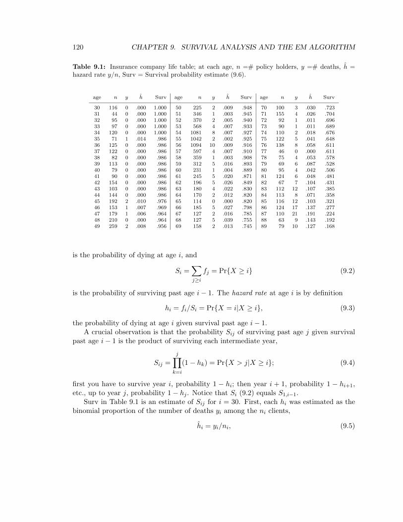
An insurance company’s life table appears in Table 9.1, showing its number of clients (thatis, life insurance policy holders) by age, and the number of deaths during the past yearin each age group,2 for example five deaths among the 312 clients age 59. The columnlabeled “Surv” is of great interest to the company’s actuaries, who have to set rates fornew policy holders. It is an estimate of survival probability: probability 0.893 of a personage 30 (the beginning of the table) surviving past age 59, etc. Surv is calculated accordingto an ancient but ingenious algorithm.

Let X represent a typical lifetime, so

fi = Pr{X = i} (9.1)

1Also known as the Mantel–Haenszel or Cochran–Mantel–Haenszel test.2The insurance company is fictitious but the deaths y are based on the true 2010 rates for US males,

per Social Security Administration data.

119

120 CHAPTER 9. SURVIVAL ANALYSIS AND THE EM ALGORITHM

Table 9.1: Insurance company life table; at each age, n =# policy holders, y =# deaths, h =hazard rate y/n, Surv = Survival probability estimate (9.6).

age n y h Surv age n y h Surv age n y h Surv

30 116 0 .000 1.000 50 225 2 .009 .948 70 100 3 .030 .72331 44 0 .000 1.000 51 346 1 .003 .945 71 155 4 .026 .70432 95 0 .000 1.000 52 370 2 .005 .940 72 92 1 .011 .69633 97 0 .000 1.000 53 568 4 .007 .933 73 90 1 .011 .68934 120 0 .000 1.000 54 1081 8 .007 .927 74 110 2 .018 .67635 71 1 .014 .986 55 1042 2 .002 .925 75 122 5 .041 .64836 125 0 .000 .986 56 1094 10 .009 .916 76 138 8 .058 .61137 122 0 .000 .986 57 597 4 .007 .910 77 46 0 .000 .61138 82 0 .000 .986 58 359 1 .003 .908 78 75 4 .053 .57839 113 0 .000 .986 59 312 5 .016 .893 79 69 6 .087 .52840 79 0 .000 .986 60 231 1 .004 .889 80 95 4 .042 .50641 90 0 .000 .986 61 245 5 .020 .871 81 124 6 .048 .48142 154 0 .000 .986 62 196 5 .026 .849 82 67 7 .104 .43143 103 0 .000 .986 63 180 4 .022 .830 83 112 12 .107 .38544 144 0 .000 .986 64 170 2 .012 .820 84 113 8 .071 .35845 192 2 .010 .976 65 114 0 .000 .820 85 116 12 .103 .32146 153 1 .007 .969 66 185 5 .027 .798 86 124 17 .137 .27747 179 1 .006 .964 67 127 2 .016 .785 87 110 21 .191 .22448 210 0 .000 .964 68 127 5 .039 .755 88 63 9 .143 .19249 259 2 .008 .956 69 158 2 .013 .745 89 79 10 .127 .168

is the probability of dying at age i, and

Si =∑j≥i

fj = Pr{X ≥ i} (9.2)

is the probability of surviving past age i− 1. The hazard rate at age i is by definition

hi = fi/Si = Pr{X = i|X ≥ i}, (9.3)

the probability of dying at age i given survival past age i− 1.A crucial observation is that the probability Sij of surviving past age j given survival

past age i− 1 is the product of surviving each intermediate year,

Sij =

j∏k=i

(1− hk) = Pr{X > j|X ≥ i}; (9.4)

first you have to survive year i, probability 1 − hi; then year i + 1, probability 1 − hi+1,etc., up to year j, probability 1− hj . Notice that Si (9.2) equals S1,i−1.

Surv in Table 9.1 is an estimate of Sij for i = 30. First, each hi was estimated as thebinomial proportion of the number of deaths yi among the ni clients,

hi = yi/ni, (9.5)

9.1. LIFE TABLES AND HAZARD RATES 121

and then setting

S30,j =

j∏k=30

(1− hk

). (9.6)

The insurance company doesn’t have to wait 50 years to learn the probability of a 30-year-old living past 80 (estimated to be 0.506 in the table). One year’s data suffices.3

Hazard rates are more often described in terms of a continuous positive random variableT (often called “time”), having density function f(t) and “reverse cdf”, or survival function,

S(t) =

∫ ∞t

f(x) dx = Pr{T ≥ t}. (9.7)

The hazard rate

h(t) = f(t)/S(t) (9.8)

satisfies

h(t)dt.= Pr {T ∈ (t, t+ dt)|T ≥ t} (9.9)

for dt→ 0, in analogy with (9.3). The analog of (9.4) is†

Pr{T ≥ t1|T ≥ t0} = exp

{−∫ t1

t0

h(x) dx

}(9.10)

so in particular the reverse cdf (9.7) is given by

S(t) = exp

{−∫ t

0h(x) dx

}. (9.11)

(As before, † indicates material discussed further in the chapter end notes.)

A one-sided exponential density

f(t) = (1/c)e−t/c for t ≥ 0 (9.12)

has S(t) = exp{−t/c} and constant hazard rate

h(t) = 1/c. (9.13)

The name “memoryless” is quite appropriate for density (9.12): having survived to anytime t, the probability of surviving dt units more is always the same, about 1 − dt/c, nomatter what t is. If human lifetimes were exponential there wouldn’t be old or youngpeople, only lucky or unlucky ones.

3Of course the estimates can go badly wrong if the hazard rates change over time.


9.2 Censored data and the Kaplan–Meier estimate

Table 9.2 reports the survival data from a randomized clinical trial run by NCOG (theNorthern California Oncology Group) comparing two treatments for head and neck cancer:Arm A, chemotherapy, versus Arm B, chemotherapy plus radiation. The response for eachpatient is survival time in months. The + sign following some entries indicates censoreddata, that is, survival times known only to exceed the reported value. There are patients“lost to followup”, mostly because the NCOG experiment ended with some of the patientsstill alive.

Table 9.2: Censored survival times in days, from two arms of NCOG study of head/neck cancer.

Arm A: Chemotherapy

7 34 42 63 64 74+ 83 84 91 108 112129 133 133 139 140 140 146 149 154 157 160160 165 173 176 185+ 218 225 241 248 273 277

279+ 297 319+ 405 417 420 440 523 523+ 583 5941101 1116+ 1146 1226+ 1349+ 1412+ 1417

Arm B: Chemotherapy+Radiation

37 84 92 94 110 112 119 127 130 133 140146 155 159 169+ 173 179 194 195 209 249 281319 339 432 469 519 528+ 547+ 613+ 633 725 759+817 1092+ 1245+ 1331+ 1557 1642+ 1771+ 1776 1897+ 2023+ 2146+

2297+

This is what the experimenters hoped to see of course, but it complicates the com-parison. Notice that there is more censoring in Arm B. In the absence of censoring wecould run a simple two-sample test, maybe Wilcoxon’s test, to see if the more aggressivetreatment of Arm B was increasing the survival times. Kaplan–Meier curves provide agraphical comparison that takes proper account of censoring. (The next section describesan appropriate censored data two-sample test.) Kaplan–Meier curves have become familiarfriends to medical researchers, a lingua franca for reporting clinical trial results.

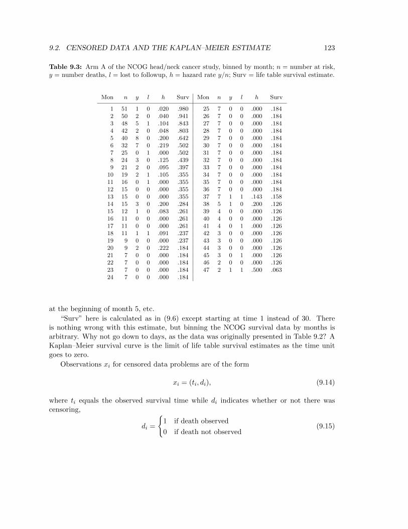
Life table methods are appropriate for censored data. Table 9.3 puts the Arm A resultsinto the same form as the insurance study of Table 9.1, now with the time unit beingmonths. Of the 51 patients enrolled4 in Arm A, y1 = 1 was observed to die in the firstmonth after treatment; this left 50 at risk, y2 = 2 of whom died in the second month;y3 = 5 of the remaining 48 died in their third month after treatment, and one was lost tofollowup, this being noted in the l column of the table, leaving n4 = 40 patients “at risk”

4The patients were enrolled at different calendar times, as they entered the study, but for each patient“time zero” in the table is set at his or her treatment.

9.2. CENSORED DATA AND THE KAPLAN–MEIER ESTIMATE 123

Table 9.3: Arm A of the NCOG head/neck cancer study, binned by month; n = number at risk,y = number deaths, l = lost to followup, h = hazard rate y/n; Surv = life table survival estimate.

Mon n y l h Surv Mon n y l h Surv

1 51 1 0 .020 .980 25 7 0 0 .000 .1842 50 2 0 .040 .941 26 7 0 0 .000 .1843 48 5 1 .104 .843 27 7 0 0 .000 .1844 42 2 0 .048 .803 28 7 0 0 .000 .1845 40 8 0 .200 .642 29 7 0 0 .000 .1846 32 7 0 .219 .502 30 7 0 0 .000 .1847 25 0 1 .000 .502 31 7 0 0 .000 .1848 24 3 0 .125 .439 32 7 0 0 .000 .1849 21 2 0 .095 .397 33 7 0 0 .000 .184

10 19 2 1 .105 .355 34 7 0 0 .000 .18411 16 0 1 .000 .355 35 7 0 0 .000 .18412 15 0 0 .000 .355 36 7 0 0 .000 .18413 15 0 0 .000 .355 37 7 1 1 .143 .15814 15 3 0 .200 .284 38 5 1 0 .200 .12615 12 1 0 .083 .261 39 4 0 0 .000 .12616 11 0 0 .000 .261 40 4 0 0 .000 .12617 11 0 0 .000 .261 41 4 0 1 .000 .12618 11 1 1 .091 .237 42 3 0 0 .000 .12619 9 0 0 .000 .237 43 3 0 0 .000 .12620 9 2 0 .222 .184 44 3 0 0 .000 .12621 7 0 0 .000 .184 45 3 0 1 .000 .12622 7 0 0 .000 .184 46 2 0 0 .000 .12623 7 0 0 .000 .184 47 2 1 1 .500 .06324 7 0 0 .000 .184

at the beginning of month 5, etc.

“Surv” here is calculated as in (9.6) except starting at time 1 instead of 30. Thereis nothing wrong with this estimate, but binning the NCOG survival data by months isarbitrary. Why not go down to days, as the data was originally presented in Table 9.2? AKaplan–Meier survival curve is the limit of life table survival estimates as the time unitgoes to zero.

Observations xi for censored data problems are of the form

xi = (ti, di), (9.14)

where ti equals the observed survival time while di indicates whether or not there wascensoring,

di =

{1 if death observed

0 if death not observed(9.15)


(so di = 0 corresponds to a + in Table 9.2). Let

t(1) < t(2) < t(3) < · · · < t(n) (9.16)

denote the ordered survival times,5 censored or not, with corresponding indicator d(k) for

t(k). The Kaplan–Meier estimate for survival probability S(j) = Pr{X > t(j)} is then†

S(j) =∏k≤j

(n− k

n− k + 1

)d(k)

. (9.17)

S jumps downward at death times tj , and is constant between observed deaths.

0 200 400 600 800 1000 1200 1400

0.0

0.2

0.4

0.6

0.8

1.0

Figure9.x. NCOG Kaplan−Meier survival curves; lower Arm A(chemo only); upper Arm B (chemo + radiation);

Vertical lines indicate approximate 95% confidence intervals

days

Sur

viva

l

Arm A

Arm B

Figure 9.1: NCOG Kaplan–Meier survival curves; lower Arm A (chemo only); upper Arm B(chemo+radiation). Vertical lines indicate approximate 95% confidence intervals.

The Kaplan–Meier curves for both arms of the NCOG study are shown in Figure 9.1.Arm B, the more aggressive treatment, looks better: its 50% survival estimate occurs at324 days, compared to 182 days for Arm A. The inferential question — is B really betterthan A or is this just random variability? — is less clear-cut.

The accuracy of S(j) can be estimated from Greenwood’s formula† for its standarddeviation (now back in life table notation),

sd(S(j)

)= S(j)

∑k≤j

yknk(nk − yk)

1/2

. (9.18)

5Assuming no ties among the survival times, which is convenient but not crucial for what follows.

9.2. CENSORED DATA AND THE KAPLAN–MEIER ESTIMATE 125

The vertical bars in Figure 9.1 are approximate 95% confidence limits for the two curvesbased on Greenwood’s formula. They overlap enough to cast doubt on the superiority ofArm B at any one choice of “days” but the two-sample test of the next section, whichcompares survival at all timepoints, will provide more definitive evidence.

Life tables and the Kaplan–Meier estimate seem like a textbook example of frequentistinference as described in Chapter 2: a useful probabilistic result is derived (9.4), and thenimplemented by the plug-in principle (9.6). There is more to the story though, as discussedbelow.

Life table curves are nonparametric, in the sense that no particular relationship isassumed between the hazard rates hi. A parametric approach can greatly improve thecurves’ accuracy.† Reverting to the life table form of Table 9.3, we assume that the deathcounts yk are independent binomials,

ykind∼ Bi(nk, hk), (9.19)

and that the logits λk = log{hk/(1− hk)} satisfy some sort of regression equation

λ = Xα, (9.20)

as in (8.22). For instance a cubic regression would have xk = (1, k, k2, k3) for the kth rowof X, with X 47× 4 for Table 9.3.

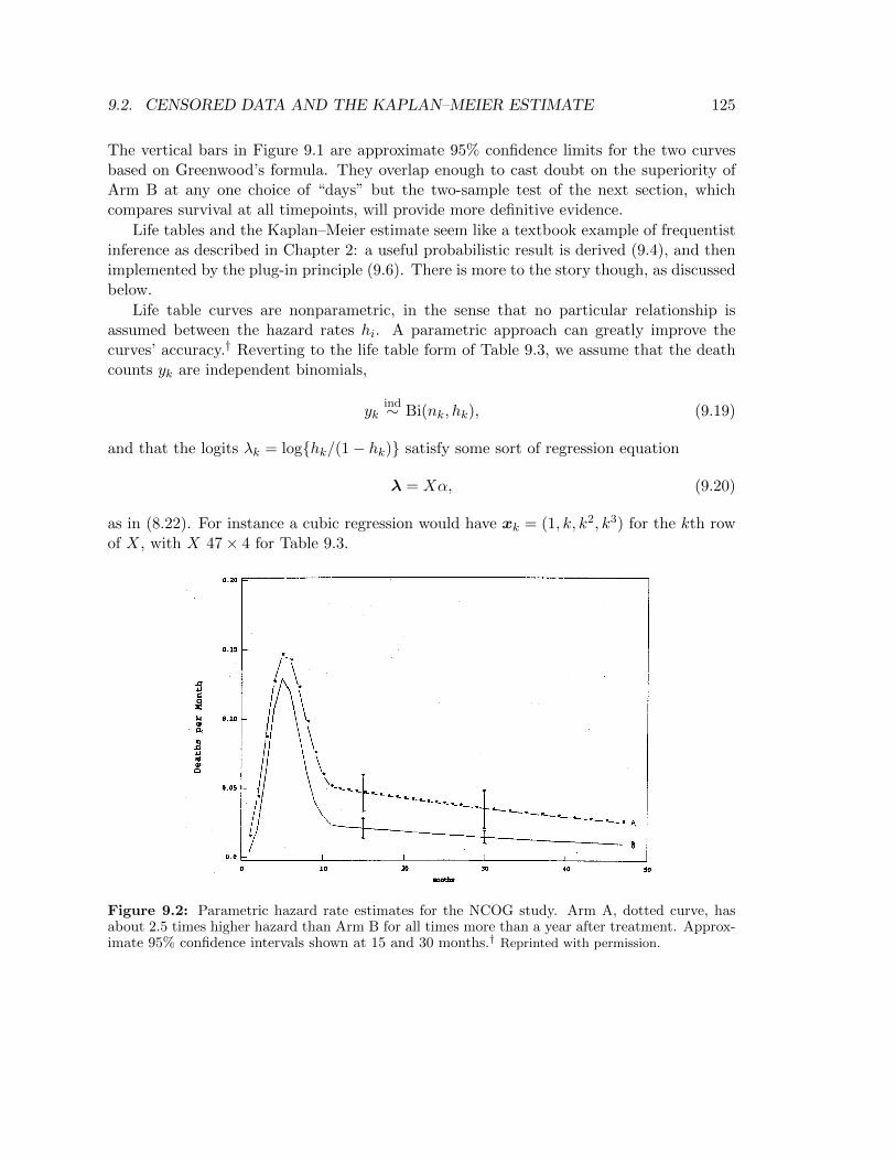
Figure 9.2: Parametric hazard rate estimates for the NCOG study. Arm A, dotted curve, hasabout 2.5 times higher hazard than Arm B for all times more than a year after treatment. Approx-imate 95% confidence intervals shown at 15 and 30 months.† Reprinted with permission.


The parametric hazard rate estimates in Figure 9.2 were instead based on a “cubic-linear spline”,

xk =(1, k, (k − 11)2

−, (k − 11)3−), (9.21)

where (k − 11)− equals k − 11 for k ≤ 11, and 0 for k ≥ 11. The vector λ = Xα describesa curve that is cubic for k ≤ 11, linear for k ≥ 11, and joined smoothly at 11. The logisticregression maximum likelihood estimate α produced hazard rate curves

hk = 1/(

1 + e−xkα)

(9.22)

as in (8.8). The dotted curve in Figure 9.2 traces hk for Arm A, while the undotted curveis that for Arm B, fit separately.

Comparison in terms of hazard rates is more informative than the survival curves ofFigure 9.1. Both arms show high initial hazards, peaking at five months, and then a longslow decline.6 Arm B hazard is always below Arm A, in a ratio of about 2.5 to 1 afterthe first year. Approximate 95% confidence limits, obtained as in (8.30), don’t overlap,indicating superiority of Arm B at 15 and 30 months after treatment.

In addition to its frequentist justification, survival analysis takes us into the Fisherianrealm of conditional inference, Section 4.3. The yk’s in model (9.19) are considered condi-tionally on the nk’s, effectively treating the nk values in Table 9.3 as ancillaries, that isas fixed constants, by themselves containing no statistical information about the unknownhazard rates. We will examine this tactic more carefully in the next two sections.

9.3 The log-rank test

A randomized clinical trial, interpreted by a two-sample test, remains as the gold standardof medical experimentation. Interpretation usually involves Student’s two-sample t-testor its nonparametric cousin Wilcoxon’s test, but neither of these are suitable for censoreddata. The log rank test† employs an ingenious extension of life tables for the nonparametrictwo-sample comparison of censored survival data.

Table 9.4 compares the results of the NCOG study for the first six months7 aftertreatment. At the beginning8 of month 1 there were 45 patients “at risk” in Arm B, noneof whom died, compared with 51 at risk and 1 death in Arm A. This left 45 at risk inArm B at the beginning of month 2, 50 in Arm A, with 1 and 2 deaths during the monthrespectively. (Losses to followup were assumed to occur at the end of each month; therewas 1 such at the end of month 3, reducing the number at risk in Arm A to 42 for month4.)

6The cubic-linear spline (9.21) is designed to show more detail in the early months, where there is moreavailable patient data and where hazard rates usually change more quickly.

7A month is defined here as 365/12 = 30.4 days.8The “beginning of month 1” is each patient’s treatment time, at which all 45 patients ever enrolled in

Arm B were at risk, that is, available for observation.

9.3. THE LOG-RANK TEST 127

Table 9.4: Life table comparison for first 6 months of NCOG study. For example, at the beginningof the 6th month after treatment, there were 33 remaining Arm B patients of whom 4 died duringthe month, compared to 32 at risk and 7 dying in Arm A. Conditional expected number of deathsin Arm A, assuming null hypothesis of equal hazard rates in both arms, was 5.42 (9.24).

MonthArm B Arm A Exp #

A deathsat risk died at risk died

1 45 0 51 1 .532 45 1 50 2 1.563 44 1 48 5 3.134 43 5 42 2 3.465 38 5 40 8 6.676 33 4 32 7 5.42

The month 6 data is displayed in two-by-two tabular form in Table 9.5, showing thenotation used in what follows: nA for the number at risk in Arm A, nd for the number ofdeaths, etc.; y indicates the number of Arm A deaths. If the marginal totals nA, nB, nd, nsare given, then y determines the other three table entries by subtraction, so we are notlosing any information by focusing on y.

Table 9.5: Two-by-two display of month 6 data for NCOG study. E is expected number of ArmA deaths assuming null hypothesis of equal hazard rates (last column of Table 9.4).

Died Survived

Ay = 7

25 nA = 32E = 5.42

B 4 29 nB = 33

nd = 11 ns = 54 n = 65

Consider the null hypothesis that the hazard rates (9.3) for month 6 are the same inArm A and Arm B,

H0(6) : hA6 = hB6. (9.23)

Under H0(6), y has mean E and variance V ,

E = nAnd/n

V = nAnBndns/ [n2(n− 1)

],

(9.24)


as calculated according to the hypergeometric distribution.† E = 5.42 and V = 2.28 inTable 9.5.

We can form a two-by-two table for each of the N = 47 months of the NCOG study,calculating yi, Ei, and Vi for month i. The log rank statistic Z is then defined to be†

Z =N∑i=1

(yi − Ei)

/(N∑i=1

Vi

)1/2

. (9.25)

The idea here is simple but clever. Each month we test the null hypothesis of equal hazardrates

H0(i) : hAi = hBi. (9.26)

The numerator yi −Ei has expectation 0 under H0(i), but if hAi is greater than hBi, thatis if treatment B is superior, then the numerator has a positive expectation. Adding up thenumerators gives us power to detect a general superiority of treatment B over A, againstthe null hypothesis of equal hazard rates, hAi = hBi for all i.

For the NCOG study, binned by months,

N∑1

yi = 42,N∑1

Ei = 32.9,N∑1

Vi = 16.0, (9.27)

giving log rank test statistic

Z = 2.27. (9.28)

Asymptotic calculations based on the central limit theorem suggest†

Z ∼ N (0, 1) (9.29)

under the null hypothesis that the two treatments are equally effective, i.e., that hAi = hBifor i = 1, 2, . . . , N . In the usual interpretation, Z = 2.27 is significant at the one-sided0.012 level, providing moderately strong evidence in favor of treatment B.

An impressive amount of inferential guile goes into the log rank test:

1. Working with hazard rates instead of densities or cdfs is essential for survival data.

2. Conditioning at each period on the numbers at risk, nA and nB in Table 9.5, finessesthe difficulties of censored data; censoring only changes the at-risk numbers in futureperiods.

3. Also conditioning on the number of deaths and survivals, nd and ns in Table 9.5,leaves only the univariate statistic y to interpret at each period, easily done throughthe null hypothesis of equal hazard rates (9.26).

9.4. THE PROPORTIONAL HAZARDS MODEL 129

4. Adding the discrepancies yi−Ei in the numerator of (9.25) (rather than say, adding

the individual Z values Zi = (yi−Ei)/V 1/2i , or adding the Z2

i ’s) accrues power for thenatural alternative hypothesis “hAi > hBi for all i”, while avoiding destabilizationfrom small values of Vi.

Each of the four tactics had been used separately in classical applications. Putting themtogether into the log rank test was a major inferential accomplishment, foreshadowing astill bigger step forward, the proportional hazards model, our subject in the next section.

Conditional inference takes on an aggressive form in the log rank test. Let Di indicateall the data except yi available at the end of the ith period. For month 6 in the NCOGstudy, D6 includes all data for months 1–5 in Table 9.4, and the marginals nA, nB, nd, nsin Table 9.5, but not the y value for month 6. The key assumption is that under the nullhypothesis of equal hazard rates (9.26),

yi|Diind∼ (Ei, Vi), (9.30)

“ind” here meaning that the yi’s can be treated as independent quantities with means andvariances (9.24). In particular, we can add the variances Vi to get the denominator of(9.25). (A “partial likelihood” argument,† described in the end notes, justifies adding thevariances.)

The purpose of all this Fisherian conditioning is to simplify the inference: the condi-tional distribution yi|Di depends only on the hazard rates hAi and hBi; “nuisance parame-ters”, relating to the survival times and censoring mechanism of the data in Table 9.2, arehidden away. There is a price to pay in testing power, though usually a small one.† Thelost-to-followup values l in Table 9.3 have been ignored, even though they might containuseful information, say if all the early losses occurred in one Arm.

9.4 The proportional hazards model

The Kaplan–Meier estimator is a one-sample device, dealing with data coming from a singledistribution. The log rank test makes two-sample comparisons. Proportional hazards upsthe ante to allow for a full regression analysis of censored data. Now the individual datapoints xi are of the form

xi = (ci, ti, di), (9.31)

where ti and di are observed survival time and censoring indicator, as in (9.14)–(9.15), andci is a known 1× p vector of covariates whose effect on survival we wish to assess. Both ofthe previous methods are included here: for the log rank test, ci indicates treatment, sayci equals 0 or 1 for Arm A or Arm B, while ci is absent for Kaplan–Meier.

Medical studies regularly produce data of form (9.31). An example, the pediatric cancerdata, is partially listed in Table 9.6. The first 20 of n = 1620 cases are shown. There arefive explanatory covariates (defined in the table’s caption): sex, race, age, calendar date of


Table 9.6: Pediatric cancer data, first 20 of 1620 children. Sex 1 = male, 2 = female; race 1 =white, 2 = nonwhite; age in years; entry = calendar date of entry in days since July 1, 2001; far =home distance from treatment center in miles; t = survival time in days; d = 1 if death observed,0 if not.

sex race age entry far t d

1 1 2.50 710 108 325 02 1 10.00 1866 38 1451 02 2 18.17 2531 100 221 02 1 3.92 2210 100 2158 01 1 11.83 875 78 760 02 1 11.17 1419 0 168 02 1 5.17 1264 28 2976 02 1 10.58 670 120 1833 01 1 1.17 1518 73 131 02 1 6.83 2101 104 2405 01 1 13.92 1239 0 969 01 1 5.17 518 117 1894 01 1 2.50 1849 99 193 11 1 .83 2758 38 1756 02 1 15.50 2004 12 682 01 1 17.83 986 65 1835 02 1 3.25 1443 58 2993 01 1 10.75 2807 42 1616 01 2 18.08 1229 23 1302 02 2 5.83 2727 23 174 1

entry into the study, and “far”, the distance of the child’s home from the treatment center.The response variable t is survival in days from time of treatment until death. Happily,only 160 of the children were observed to die (d = 1). Some left the study for variousreasons, but most of the d = 0 cases were those children still alive at the end of the studyperiod. Of particular interest was the effect of “far” on survival. We wish to carry out aregression analysis of this heavily censored data set.

The proportional hazards model assumes that the hazard rate hi(t) for the ith individual(9.8) is

hi(t) = h0(t)eciβ. (9.32)

Here h0(t) is a baseline hazard (which we need not specify) and β is an unknown p-parameter vector we want to estimate. For concise notation, let

θi = eciβ; (9.33)

model (9.32) says that individual i’s hazard is a constant factor θi times the baseline hazard.Equivalently, from (9.11), the ith survival function Si(t) is a power of the baseline survival

9.4. THE PROPORTIONAL HAZARDS MODEL 131

function S0(t),

Si(t) = S0(t)θi . (9.34)

Larger values of θi lead to more quickly declining survival curves, i.e., to worse survival.

Let J be the number of observed deaths, J = 160 here, occurring at times

T(1) < T(2) < · · · < T(J), (9.35)

again for convenience assuming no ties.9 Just before time T(j) there is a risk set of indi-viduals still under observation, whose indices we denote by Rj ,

Rj = {i : ti ≥ T(j)}. (9.36)

Let ij be the index of the individual observed to die at time T(j). The key to proportionalhazards regression is the following result.

Lemma. † Under the proportional hazards model (9.32), the conditional probability, giventhe risk set Rj, that individual i in Rj is the one observed to die at time T(j) is

Pr{ij = i|Rj} = eciβ/ ∑

k∈Rj

eckβ. (9.37)

To put it in words, given that one person dies at time T(j), the probability it is individuali is proportional to exp(ciβ), among the set of individuals at risk.

For the purpose of estimating the parameter vector β in model (9.32), we multiplyfactors (9.37) to form the partial likelihood

L(β) =J∏j=1

ecijβ/ ∑k∈Rj

eckβ

. (9.38)

L(β) is then treated as an ordinary likelihood function, yielding an approximately unbiasedMLE-like estimate

β = arg maxβ{L(β)} , (9.39)

with an approximate covariance obtained from the second derivative matrix† of l(β) =logL(β), as in Section 4.3,

β ∼(β,[−l(β)]−1

). (9.40)

9More precisely, assuming only one event, a death, occured at T(j), with none of the other individualsbeing lost to followup at exact time T(j).


Table 9.7: Proportional hazards analysis of pediatric cancer data (with age, entry and far stan-dardized). Age is significantly negative, older children doing better; entry is very significantlynegative, showing a declining hazard rate with calendar date of entry; far is very significantly pos-itive, indicating worse results for children living farther away from the treatment center. Last twocolumns show limits of approximate 95% confidence intervals for exp(β).

β sd z-val p-val exp(β) lo up

sex −.023 .160 −.142 .887 .98 .71 1.34race .282 .169 1.669 .095 1.33 .95 1.85age −.235 .088 −2.664 .008** .79 .67 .94entry −.460 .079 −5.855 .000*** .63 .54 .74far .296 .072 4.117 .000*** 1.34 1.17 1.55

Table 9.7 shows the proportional hazards analysis of the pediatric cancer data, withthe covariates age, entry, and far standardized to have mean 0 and standard deviation 1for the 1620 cases.10 Neither sex nor race seems to make much difference. We see that ageis a mildly significant factor, with older ages doing better (i.e., the estimated regressioncoefficient is negative). However, the dramatic effects are from date of entry and “far”.Individuals who entered the study later survived longer — perhaps the treatment protocolwas being improved — while children living farther away from the treatment center didworse.

Justification of the partial likelihood calculations is similar to that for the log ranktest, but there are some important differences, too: the proportional hazards model issemiparametric (“semi” because we don’t have to specify h0(t) in (9.31)), rather thannonparametric as before; and the emphasis on likelihood has increased the Fisherian natureof the inference, moving it further away from pure frequentism. Still more Fisherian isthe emphasis on likelihood inference in (9.38)–(9.40), rather than the direct frequentistcalculations of (9.24)–(9.25).

The conditioning argument here is less obvious than that for the Kaplan–Meier estimateof the log rank test. Has its convenience possibly come at too high a price? In fact it canbe shown† that inference based on the partial likelihood is highly efficient, assuming ofcourse the correctness of the proportional hazards model (9.31).

9.5 Missing data and the EM algorithm

Censored data, the motivating factor for survival analysis, can be thought of as a specialcase of a more general statistical topic, missing data. What’s missing, in Table 9.2 forexample, are the actual survival times for the + cases, which are known only to exceed the

10Table 9.7 obtained using R program coxph.

9.5. MISSING DATA AND THE EM ALGORITHM 133

tabled values. If the data were not missing, we could use standard statistical methods, forinstance Wilcoxon’s test, to compare the two arms of the NCOG study. The EM algorithmis an iterative technique for solving missing data inferential problems using only standardmethods.

*

*

*

*

*

*

*

*

*

**

*

** *

*

*

*

*

*

** * * **** ***** ** ** ** *

0 1 2 3 4 5

−0.

50.

00.

51.

01.

52.

02.

5Figure 9.3. 40 points from a binomial normal distribution,

the last 20 with x[2] missing (circled)

x[1]

x[2]

●● ● ● ●●●● ●●●●● ●● ●● ●● ●

Figure 9.3: 40 points from a binomial normal distribution, the last 20 with x[2] missing (circled).

A missing data situation is shown in Figure 9.3: n = 40 points have been independentlysampled from a bivariate normal distribution (5.12), means (µ1, µ2), variances (σ2

1, σ22), and

correlation ρ, (x1i

x2i

)ind∼ N2

((µ1

µ2

),

(σ2

1 σ1σ2ρ

σ1σ2ρ σ22

)). (9.41)

However, the second coordinates of the last 20 points have been lost. These are representedby the circled points in Figure 9.3, with their x2 values arbitrarily set to 0.

We wish to find the maximum likelihood estimate of the parameter vector θ = (µ1, µ2,σ1, σ2, ρ). The standard maximum likelihood estimates

µ1 =

40∑1

x1i/40, µ2 =

40∑1

x2i/40,

σ1 =

[40∑1

(x1i − µ1)2 /40

]1/2

, σ2 =

[40∑1

(x2i − µ2)2 /40

]1/2

,

ρ =

[40∑1

(x1i − µ1) (x2i − µ2) /40

]/(σ1σ2) ,

(9.42)


Table 9.8: EM algorithm for estimating means, standard deviations, correlation of the bivariatenormal distribution that gave data in Figure 9.3.

Step µ1 µ2 σ1 σ2 ρ

1 1.86 .463 1.08 .738 .1622 1.86 .707 1.08 .622 .3943 1.86 .843 1.08 .611 .5744 1.86 .923 1.08 .636 .6795 1.86 .971 1.08 .667 .7366 1.86 1.002 1.08 .694 .7697 1.86 1.023 1.08 .716 .7898 1.86 1.036 1.08 .731 .8019 1.86 1.045 1.08 .743 .808

10 1.86 1.051 1.08 .751 .81311 1.86 1.055 1.08 .756 .81612 1.86 1.058 1.08 .760 .81913 1.86 1.060 1.08 .763 .82014 1.86 1.061 1.08 .765 .82115 1.86 1.062 1.08 .766 .82216 1.86 1.063 1.08 .767 .82217 1.86 1.064 1.08 .768 .82318 1.86 1.064 1.08 .768 .82319 1.86 1.064 1.08 .769 .82320 1.86 1.064 1.08 .769 .823

are unavailable with missing data.The EM algorithm begins by filling in the missing data in some way, say by setting

x2i = 0 for the 20 missing values, giving an artificially complete data set datao. Then:

• The standard method (9.42) is applied to datao to produce θo = (µo1, µo2, σ

o1, σ

o2, ρ

o);this is the M (“maximizing”) step.

• Each of the missing values is replaced by its conditional expectation (assuming θ = θo)given the nonmissing data; this is the E (“expectation”) step. In our case the missingvalues x2i are replaced by

µ(0)2 +

σ(0)2

σ(0)1

(x1i − µ(0)

1

). (9.43)

• The E and M steps are repeated, at the jth stage giving a new artificially completedata set data(j) and an updated estimate θ(j). The iteration stops when ‖θ(j)+1−θ(j)‖is suitably small.

Table 9.8 shows the EM algorithm at work on the bivariate normal example of Fig-ure 9.3. In exponential families the algorithm is guaranteed to converge to the MLE θ

9.5. MISSING DATA AND THE EM ALGORITHM 135

based on just the observed data o; moreover, the likelihood fθ(j)(o) increases with everystep j. (The convergence can be sluggish, as it is here for σ2 and ρ.)

The EM algorithm ultimately derives from the fake data principle,† a property of max-imum likelihood estimation going back to Fisher. Let x = (o,u) represent the “completedata”, of which o is observed while u is unobserved or missing. Write the density for x as

fθ(x) = fθ(o)fθ(u|o), (9.44)

and let θ(o) be the MLE of θ based just on o.

Suppose we now generate simulations of u by sampling from the conditional distributionfθ(o)(u|o),

u∗k ∼ fθ(o)(u|o) for k = 1, 2, . . . ,K (9.45)

(the stars indicating creation by the statistician and not by observation), giving fakecomplete-data values x∗k = (o,u∗k). Let

data∗ = {x∗1,x∗2, . . . ,x∗K}, (9.46)

whose notional likelihood∏K

1 fθ(x∗k) yields MLE θ∗. It then turns out that θ∗ goes

to θ(o) as K goes to infinity. In other words, maximum likelihood estimation is self-consistent : generating artificial data from the MLE density fθ(o)(u|o) doesn’t change the

MLE. Moreover, any value θ(0) not equal to the MLE θ(o) is not self-consistent†: carryingthrough (9.45)–(9.46) using fθ(0)(u|o) leads to hypothetical MLE θ(1) having fθ(1)(o) >fθ(0)(o) etc., a more general version of the EM algorithm.11

Modern technology allows social scientists to collect huge data sets, perhaps hundreds ofresponses for each of thousands or even millions of individuals. Inevitably, some entries ofthe individual responses will be missing. Imputation amounts to employing some versionof the fake data principle to fill in the missing values. Imputation’s goal goes beyondfinding the MLE, to the creation of graphs, confidence intervals, histograms, and more,using convenient, standard complete-data methods.

Finally, returning to survival analysis, the Kaplan–Meier estimate (9.17) is itself self-consistent.† Consider the Arm A censored observation 74+ in Table 9.2. We know that thatpatient’s survival time exceeded 74. Suppose we distribute his probability mass (1/51 ofthe Arm A sample) to the right, in accordance with the conditional distribution for x > 74defined by the Arm A Kaplan–Meier survival curve. It turns out that redistributing all thecensored cases does not change the original Kaplan–Meier survival curve; Kaplan–Meieris self-consistent, leading to its identification as the “nonparametric MLE” of a survivalfunction.

11Simulation (9.45) is unnecessary in exponential families, where at each stage data∗ can be replaced by(o, E(j)(u|o)), E(j) indicating expectation with respect to θ(j), as in (9.43).


9.6 Notes and details

The progression from life tables, Kaplan–Meier curves, and the log rank test to propor-tional hazards regression was modest in its computational demands, until the final step.Kaplan–Meier curves and log rank tests lie within the capabilities of mechanical calcula-tors. Not so for proportional hazards, which is emphatically a child of the computer age.As the algorithms grew more intricate, their inferential justification deepened in scope andsophistication. This is a pattern we also saw in Chapter 8, in the progression from bioassayto logistic regression to generalized linear models, and will reappear as we move from thejackknife to the bootstrap in Chapter 10.

This chapter featured an all-star cast, including four of the most referenced papers ofthe post-war era: Kaplan and Meier (1958), Cox (1972) on proportional hazards, Dempster,Laird and Rubin (1977) codifying and naming the EM algorithm, and Mantel and Haenszel(1959) on the log rank test. The not very helpful name “log rank” does at least remind usthat the test depends only on the ranks of the survival times, and will give the same result

if all the observed survival times ti are monotonically transformed, say to exp(ti) or t1/2i .

It is often referred to as the Mantel–Haenszel or Cochran–Mantel–Haenszel test in olderliterature. Kaplan–Meier and proportional hazards are also rank-based procedures.

Censoring is not the same as truncation. For the truncated galaxy data of Section 8.3,we only learn of the existence of a galaxy if it falls into the observation region (8.39).The censored individuals in Table 9.2 are known to exist, but with imperfect knowledge oftheir lifetimes. There is a version of the Kaplan–Meier curve applying to truncated data,developed in the astronomy literature by Lynden-Bell (1971).

The methods of this chapter apply to data that is left-truncated as well as right-censored. In a survival time study of a new HIV drug, for instance, subject i might notenter the study until some time τi after his or her initial diagnosis, in which case ti wouldbe left-truncated at τi, as well as possibly later right-censored. This only modifies thecomposition of the various risk sets. However other missing data situations, e.g., left- andright-censoring, require more elaborate, less elegant, treatments.

Formula (9.10) Let the interval [t0, t1] be partitioned into a large number of subintervalsof length dt, with tk the midpoint of subinterval k. As in (9.4), using (9.9),

Pr{T ≥ t1|T ≥ t0}.=∏

(1− h(ti)dt)

= exp{∑

log (1− h(ti)dt)}.= exp

{−∑

h(ti)dt},

(9.47)

which, as dt→ 0, goes to (9.10).

Kaplan–Meier estimate In the life table formula (9.6) (with k = 1), let the time unit besmall enough to make each bin contain at most one value t(k) (9.16). Then at t(k),

h(k) =d(k)

n− k + 1, (9.48)

9.6. NOTES AND DETAILS 137

giving expression (9.17).

Greenwood’s formula (9.18) In the life table formulation of Section 9.1, (9.6) gives

log Sj =

j∑1

log(

1− hk). (9.49)

From hkind∼ Bi(nk, hk) we get

var{

log Sj

}=

j∑1

var{

log(

1− hk)}

.=

j∑1

var hk(1− hk)2

=

j∑1

hk1− hk

1

nk,

(9.50)

where we have used the delta-method approximation var{logX} .= var{X}/E{X}2. Plug-ging in hk = yk/nk yields

var{

log Sj

}.=

j∑1

yknk(nk − yk)

. (9.51)

Then the inverse approximation var{X} = E{X}2 var{logX} gives Greenwood’s formula(9.18).

The censored data situation of Section 9.2 does not enjoy independence between thehk values. However, successive conditional independence, given the nk values, is enoughto verify the result, as in the partial likelihood calculations below. Note: the confidenceintervals in Figure 9.1 were obtained by exponentiating the intervals,

log Sj ±[1.96 var

{log Sj

}]1/2. (9.52)

Parametric life tables analysis Figure 9.2 and the analysis behind it is developed in Efron(1988), where it is called “partial logistic regression” in analogy with partial likelihood.

Hypergeometric distribution Hypergeometric calculations, as for Table 9.5, are oftenstated as follows: n marbles are placed in an urn, nA labeled A and nB labeled B; ndmarbles are drawn out at random; y is the number of these labeled A. Elementary (butnot simple) calculations then produce the conditional distribution of y given the table’smarginals nA, nB, n, nd, ns,

Pr{y|marginals} =

(nAy

)(nB

nd − y

)/(n

nd

)(9.53)


for

max(nA − ns, 0) ≤ y ≤ min(nd, nA),

and expressions (9.24) for the mean and variance. If nA and nB go to infinity such thatnA/n→ pA and nB/n→ 1− pA, then V → ndpA(1− pA), the variance of y ∼ Bi(nd, pA).

Log rank statistic Z (9.25) Why is (∑N

1 Vi)1/2 the correct denominator for Z? Let

ui = yi − Ei in (9.30), so Z’s numerator is∑N

1 ui, with

ui|Di ∼ (0, Vi) (9.54)

under the null hypothesis of equal hazard rates. This implies that, unconditionally, E{ui} =0. For j < i, uj is a function of Di (since yj and Ej are), so E{ujui|Di} = 0, and againunconditionally, E{ujui} = 0. Therefore, assuming equal hazard rates,

E

(N∑1

ui

)2

= E

(N∑1

u2i

)=

N∑1

var{ui}

.=

N∑1

Vi.

(9.55)

The last approximation, replacing unconditional variances var{ui} with conditional vari-ances Vi is justified in Crowley (1974), as is the asymptotic normality (9.29).

Lemma (9.37) For λ ∈ Rj , the probability pi that death occurs in the infinitesimalinterval (T(j), T(j) + dT ) is hi(T(j))dT , so

pi = h0(T(j))eciβdT, (9.56)

so the probability of event Ai that individual i dies while the others don’t is

Pi = pi∏

k∈Rj−i(1− pk). (9.57)

But the Ai are disjoint events, so given that ∪Ai has occured, the probability that it isindividual i who died is

Pi

/∑Rj

Pj.= eciβ

/ ∑k∈Rj

eckβ, (9.58)

this becoming exactly (9.37) as dT → 0.

Partial likelihood (9.40) Cox (1975) introduced partial likelihood as inferential justifica-tion for the proportional hazards model, which had been questioned in the literature. LetDj indicate all the observable information available just before time T(j)(9.35), including

9.6. NOTES AND DETAILS 139

all the death or loss times for individuals having ti < T(j). (Notice that Dj determines therisk set Rj .) By successive conditioning we write the full likelihood fθ(data) as

fθ(data) = fθ(D1)fθ(i1|R1)fθ(D2|D1)fθ(i2|R2) · · ·

=J∏j=1

fθ(Dj |Dj−1)J∏j=1

fθ(ij |Rj).(9.59)

Letting θ = (α, β), where α is a nuisance parameter vector having to do with the occurrenceand timing of events between observed deaths,

fα,β(data) =

J∏j=1

fα,β(Dj |Dj−1)

L(β), (9.60)

where L(β) is the partial likelihood (9.38).The proportional hazards model simply ignores the bracketed factor in (9.60); l(β) =

logL(β) is treated as a genuine likelihood, maximized to give β, and assigned covariancematrix (−l(β))−1 as in Section 4.3. Efron (1977) shows this tactic is highly efficient for theestimation of β.

Fake data principle For any two values of the parameters θ1 and θ2 define

lθ1(θ2) =

∫[log fθ2(o,u)] fθ1(u|o) du, (9.61)

this being the limit as K →∞ of the fake data log likelihood (9.46) under θ2,

lθ1(θ2) = limK→∞

1

K

K∑k=1

log fθ2(o,u∗k) (9.62)

if θ1 were the true value of θ. Using fθ(o,u) = fθ(o)fθ(u|o), definition (9.61) gives

lθ1(θ2)− lθ1(θ1) = logfθ2(o)

fθ1(o)−∫ (

logfθ2(u|o)

fθ1(u|o)

)fθ1(u|o)

= logfθ2(o)

fθ1(o)− 1

2D (fθ1(u|o), fθ2(u|o)) ,

(9.63)

with D the deviance (8.31), always postive unless u|o has the same distribution under θ1

and θ2, which we will assume doesn’t happen.Suppose we begin the EM algorithm at θ = θ1 and find the value θ2 maximizing

lθ1(θ). Then lθ1(θ2) > lθ2(θ1) and D > 0 implies fθ2(o) > fθ1(o) in (9.63); that is, wehave increased the likelihood of the observed data. Now take θ1 = θ = arg maxθ fθ(o).Then the right side of (9.63) is negative, implying lθ(θ) > lθ(θ2) for any θ2 not equaling θ1.


Putting this together,12 successively computing θ1, θ2, θ3, . . . by fake data MLE calculationsincreases fθ(o) at every step, and the only stable point of the algorithm is at θ = θ(o).

Kaplan–Meier self-consistency This property was verified in Efron (1967), where thename was coined.

12Generating the fake data is equivalent to the E step of the algorithm, the M step being the maximizationof lθj (θ).

survival analysis and the em algorithm - home |...

Documents