surveying the landscape: an in-depth analysis of spatial

Surveying the Landscape:An In-Depth Analysis of Spatial Database Workloads

Bogdan SimionDept. of Computer Science

University of [email protected]

Suprio RayDept. of Computer Science


Angela Demke BrownDept. of Computer Science


ABSTRACTSpatial databases are increasingly important for a wide variety ofreal-world applications, such as land surveying, urban planning,cartography and location-based services. However, spatial databaseworkload properties are not well-understood. For example, it isunknown to what degree one spatial application resembles anotherin terms of resource demand, or how the demand will change asmore concurrent queries (i.e., more users) are added. We show thatspatial workloads have a different CPU execution profile than well-studied decision support workloads, as represented by TPC-H.

We present a framework to automatically classify spatial queriesand characterize spatial workload mixes. We first analyze the re-source consumption (i.e., computation and I/O) of a representativeset of spatial queries, which are then classified into five distinctcategories. Next, we create five homogeneous spatial workloads,each composed of queries from one of these classes. We thenvary database-specific parameters (e.g., the buffer pool size) andworkload specific parameters (e.g., the query mix), to characterizea workload in terms of CPU utilization and I/O activity trends.

We study workloads simulating real-world spatial database ap-plications and show how our framework can classify them and pre-dict resource utilization trends under various settings. This can pro-vide clues to the database administrator regarding which resourcesare heavily contended and can guide resource upgrades. We furthervalidate our approach by applying it to a much larger dataset, andto a second DBMS.

Categories and Subject DescriptorsH.2.8 [Database Applications]: Spatial databases and GIS; H.3.4[Systems and Software]: Performance evaluation

General TermsPerformance, Measurement

KeywordsQuery classification, workload characterization, architectural stallbreakdown, PostGIS, Informix

Permission to make digital or hard copies of all or part of this work forpersonal or classroom use is granted without fee provided that copies arenot made or distributed for profit or commercial advantage and that copiesbear this notice and the full citation on the first page. To copy otherwise, torepublish, to post on servers or to redistribute to lists, requires prior specificpermission and/or a fee. ACM SIGSPATIAL GIS ’12, November 6-9, 2012.Redondo Beach, CA, USACopyright c© 2012 ACM ISBN 978-1-4503-1691-0/12/11 ...$15.00.

1. INTRODUCTIONSpatial database workloads are increasingly important, thanks

to the advent of popular geospatial Web services such as GoogleMaps, in-vehicle GPS navigation systems, and a host of accompa-nying location-based services. Other important geospatial applica-tions include city planning, land surveys and environment assess-ments. Most relational database systems now offer spatial features.

As uses of spatial databases become more widespread, there is agrowing need to analyze and understand the characteristics of dif-ferent spatial applications. The characterization of database work-loads is pivotal in analyzing performance issues, detecting opti-mization opportunities and determining how well the system willscale as data volume and request rate increases. Workload charac-terization can also enable automatic tuning of databases, therebyreducing the cost and complexity of database management [25].

Workload characterization is the quantitative description of aworkload with the objective of obtaining a model that encapsulatesits essential features and dynamic behavior [5]. Often, such work-load analysis is conducted informally by the Database Adminis-trators (DBAs), who study query plans and try various ad hoc so-lutions to improve the performance of a query (e.g., by rewritingit or by tuning various system parameters on a trial-and-error ba-sis). This reliance on DBA expertise is costly, and does not easilytranslate to new situations. Although several research projects havestudied how to characterize database workloads [10] [11] [12], theyhave mainly focused on TPC [23] workloads such as OLTP (On-line Transaction Processing) and DSS (Decision Support System).

To date, there has been no such characterization of spatial databaseworkloads, making it difficult to answer even relatively simple ques-tions. For instance, to what extent does one spatial application re-semble another in terms of its resource demand? What optimiza-tions or hardware upgrades will be most beneficial for a given appli-cation? To address such questions, we “survey” the spatial queryexecution landscape1. We present a framework to automaticallyclassify spatial queries by the nature of their resource consumption(computationally intensive, data intensive, mixed, low resource uti-lization etc.) and characterize spatial workload mixes. Based ona series of factors, our framework can provide clues to the users(or DBAs) in a reactive manner, to offer a better understanding ofwhich resources are heavily utilized. Furthermore, we analyze howthis resource pressure changes with parameters such as the bufferpool size and query density in the workload mix.

Our goal is to identify the inherent resource demands of thequeries that make up a workload, enabling the prediction of per-formance trends as hardware and workload intensity changes. Weaim to minimize the number of measurements that are needed to

1We draw an analogy to land surveying, which uses measurementsto establish the relative position of physical features on the earth.

characterize a new target workload. Our contributions are:

1. We demonstrate that spatial queries differ from previously ana-lyzed decision support workloads (as represented by TPC-H), interms of their low-level CPU characteristics such as instructionand data cache misses and branch mispredictions.

2. We analyze the resource utilization of spatial queries and deter-mine their nature in terms of the computation and data accessesthey perform (i.e., compute-intensive, data-intensive, mixed, low-resource utilization etc.). We show that queries can be classifiedinto five distinct categories.

3. We extend the Jackpine spatial database benchmark [19] with amechanism to create custom concurrent spatial workloads. Weuse this to construct five custom workloads, each composedof multiple concurrent queries drawn from one of the queryclasses, and characterize them by varying parameters such asthe buffer pool size and the query density. We show how eachclass of workload reacts to these changes.

4. We show how the query classification and the characterizationsof known homogeneous workloads can be used to classify newworkloads and predict their behavior under varying conditions.We demonstrate this on a set of realistic applications simulatedin the Jackpine macrobenchmark suite.

The rest of the paper is organized as follows. Section 2 presentsbackground on spatial databases and the benchmarks that we use.Next, Section 3 explores the CPU and I/O behavior of spatial queriesto motivate our framework for query classification and spatial work-load characterization, which is presented in Section 4. We demon-strate the use of this framework, showing how it can predict trendsin previously unseen workloads, in Section 5. Using a secondDBMS and a larger dataset, we validate our methodology in Sec-tion 6. Related work and conclusions are in Sections 7 and 8.

2. BACKGROUND ON METHODOLOGYIn this section, we present some background on spatial databases

and testing considerations that influence our methodology.There are a wide variety of geospatial databases, ranging from

open-source projects such as MySQL and PostGIS (the spatial ex-tension to PostgreSQL) to commercial products such as OracleSpatial, ArcGIS and Informix. These databases contain built-insupport for spatial data types (e.g., point, line, polygon) and spa-tial operations (e.g., distance, intersects, contains, etc.) that canbe performed on the data shapes. The Open Geospatial Consor-tium (OGC) [17] recently standardized the set of spatial operationsthat should be provided in any geospatial database, however manyproducts are not yet OGC-compliant. For example, MySQL lackssupport for spatial operations like ST_Distance and ST_Dwithin.

Spatial query processing, which is a two-step process comprisedof filtering and refinement stages, also differs across spatial databases.In the filtering step, the records are filtered based on the minimumbounding rectangles (MBRs) of the data shapes, to narrow downthe possible matches to a much smaller candidate result set. Inthe refinement step, the records in the candidate result set are pro-cessed to determine which shapes satisfy the spatial criteria. Mostdatabases comply with this two-step evaluation. However, some(e.g. MySQL) only perform the filtering stage, which can lead tomany false positives in the final result set.

For our purposes, we wish to experiment with an implementationthat is OGC-compliant, performs both stages of the spatial queryprocessing, and is open source to allow us to investigate the causesfor the behavior we observe. These requirements lead us to selectPostgreSQL with the PostGIS extension as our target database.

In our analysis we use read-only workloads. From our expe-rience with spatial databases, we observed that many real-worldspatial applications involve read-mostly workloads and updates arevery infrequent. For example, datasets representing cartographicmaps, land ownership information, and flood insurance rate mapsare rarely updated but are heavily queried. Although certain appli-cations such as those involving spatio-temporal workloads do in-volve frequent updates, our current analysis has not addressed thesescenarios. Extending the workload characterization to update-heavyapplications is an important avenue for future work.

For test queries and datasets, we use the open-source Jackpinespatial database benchmark [19]. Jackpine provides comprehen-sive coverage of common spatial operators and several representa-tive spatial application scenarios. In its initial version, Jackpine didnot support multiple concurrent scenarios of different types, so wemodified it to add support for concurrent heterogeneous query exe-cution. We use this implementation to drive our spatial workloads.Jackpine uses the TIGER [22] dataset for the state of Texas and afew additional datasets corresponding to Travis County and the cityof Austin [7]. These datasets have a variety of spatial features. Thecardinality of the largest table is roughly 6 million records (requir-ing 1.7GB of storage for data and 400MB for spatial index) con-taining line shapes representing roads and rivers. We also added anadditional copy of each data table to artificially inflate the spatialdataset size. The total dataset size is slightly under 9GB, includingdata tables and indices.

3. SPATIAL DATABASE RESOURCE USAGESpatial and non-spatial databases use several system resources

during query execution, such as the CPU (for computation), andthe disk (for retrieving data records). Another common trait is theimpact of buffer pool size on database performance, since obvi-ously more cache means that more data can fit into memory andmore expensive disk accesses can be avoided.

There are, however, key differences that distinguish spatial andnon-spatial databases. First, spatial queries must evaluate spatialrelationships between shapes, involving complex geometric com-putations that can saturate the CPU for a long time. Second, geo-metric shapes do not have a fixed length, making the storage of spa-tial data more complicated. For example, the polygon for Maine ismuch larger than the one for Wyoming, which is a simple rectangle.Thus, spatial data must be stored in variable-length fields, whichcreates problems with record alignment. PostgreSQL’s solution isto store large shapes (such as lines and polygons) as TOAST2 datablocks, which are kept separate from the other fields in the maintable. A TOAST index allows fast access to TOAST data blocks.

We first examine how these differences affect spatial query pro-cessing in terms of the CPU time breakdown for an in-memorydataset, before considering the effect of I/O.

3.1 Comparison of architecture-level eventsSpatial applications and their associated data and queries involve

a different type of processing, which imposes a different stress onsystem resources. An architectural breakdown of the CPU process-ing time illustrates these differences for two standard sets of spatialand non-spatial analytical queries.

We compare the set of microbenchmark queries from Jackpine,and those from the non-spatial TPC-H benchmark, on the same ma-chine. Both benchmarks include a large set of read-only queries, in-volving a variety of complex analytical operations. In both bench-marks, there are long-running and short-running queries, and both

2TOAST stands for “The Oversized-Attribute Storage Technique”

0

10

20

30

40

50

60

70

80

90

100

1 2 3 4 5 6 7 8 91

01

11

21

31

41

51

61

71

81

92

02

12

22

32

42

52

62

72

82

93

0A

VG

% e

xe

cu

tio

n t

ime

Spatial queries

mispred

L2

dTLB

L1D

iTLB

L1I

(a) Spatial benchmark

0

10

20

30

40

50

60

70

80

90

100

1 2 3 4 5 6 7 8 9

10

11

12

13

14

16

17

18

19

20

21

22

AV

G

% e

xe

cu

tio

n t

ime

TPC-H queries

mispred

L2

dTLB

L1D

iTLB

L1I

(b) TPC-H benchmark

Figure 1: Architectural breakdown for spatial and non-spatial workloads

involve complex query plans, with sequential scans, index scans,joins and other typical relational operators. Both test datasets areroughly equal in size, with multiple large data tables and indexes.

To eliminate I/O effects and focus on the CPU, we ensure thatdata is entirely memory resident by warming up main memory andcaches with multiple runs for each query. Additionally, to deter-mine the confidence intervals we repeated the experiments severaltimes and found that the average variation is less than 4%.

To show the dominant components of the CPU processing timeduring query execution, we use an approach similar to Ailamaki etal. [1], who showed that for some database workloads CPU stallsare a big component of execution time. We measure several eventsthat can cause CPU stalls: L1 data and L1 instruction cache misses,L2 cache misses, data and instruction TLB misses, and branch mis-predictions. We then use a fixed cost estimate for each event to givea breakdown in terms of execution time. This is an approximation,since several stall events may overlap in time.

These events can be obtained using hardware performance coun-ters available in most modern CPUs. The performance analysistool "perf", included in Linux kernels, can monitor and record thesecounters. It provides a detailed report on the number of occurrencesfor each event. The cache and TLB latencies for our hardware areestimated using the Calibrator tool [4]. Branch misprediction la-tencies are estimated based on our processor specifications.

After running the spatial queries from Jackpine and non-spatialqueries from TPC-H through the PostgreSQL engine, we show aside-by-side comparison in Figure 1. Since the queries in Jackpinehad long descriptions, we ordered them alphabetically and num-bered them for easy reference in the figures. We also omitted query15 from TPC-H since it involves creating a view which is not typi-cal of other TPC-H and spatial queries. The final bar in each graphshows the average contribution to execution time for each of thefeatures analyzed, for both spatial and TPC-H queries. We noteseveral interesting differences.

First, spatial queries incur fewer cache misses on average thantheir non-spatial counterparts. However, spatial queries spend morethan twice the execution time (3.6%) in L1 instruction cache missescompared to TPC-H queries (1.5%). A few spatial queries (3, 8and 25) involve a materialization with sequential scan on the outerrelation of the join, which causes a much higher L1 instruction missrate than others. Even if we exclude the 3 outliers, spatial queriesstill spend roughly 1.6 times more execution time in L1 instructionmisses than TPC-H queries. As for L1 data cache misses, theyaccount for less than 7% of execution time on average for spatialqueries, compared to a whopping 19% for TPC-H queries. TheL2 misses are also higher on average for TPC-H queries (roughly5% of execution time) compared to spatial queries (less than 1% of

execution time).Second, spatial queries incur a slightly lower number of data and

instruction TLB misses than non-spatial ones (2.4% of executiontime on average for spatial queries, compared to 3% for TPC-H).

Third, spatial queries incur a lot more branch mispredictions,which can be very expensive since fetching the wrong instructionspollutes the caches with unnecessary instructions and causes stallsdue to pipeline flushes. Branch mispredictions account for 8% ofthe execution time on average for spatial queries, compared to ap-proximately 4.5% for TPC-H queries.

Overall, spatial queries are a lot more “CPU-friendly”: a greaterportion of execution time is spent performing useful computations,rather than stalling. Consequently, we argue that spatial workloadsare a beast of a different nature, and thus warrant special attention.

3.2 Characterization of I/O behaviorAt the other end of the spectrum from the CPU, database query

processing requires I/O. Thus, we examined the I/O behavior, asseen at the disk level, during spatial query processing. To capturethe complete I/O behavior we only use cold runs so that the data isnot already cached in memory.

The Jackpine microbenchmark includes spatial join and spatialanalysis functions. The spatial join queries (all pair join and joinwith a given spatial object) involve accessing multiple on-disk files,such as the corresponding data files, index files, the TOAST datafiles and TOAST index files. Due to the interleaved accesses tothese files, the disk throughput of these queries resembles that ofa random access pattern. The spatial analysis functions operate onone table and require accessing the corresponding data file, TOASTdata file and TOAST index file only. These queries achieved diskthroughput that resembles sequential access. This I/O behavior isexpected, given the organization of the database files and the char-acteristics of disk drives.

3.3 Combined resource utilizationWe now consider the combined demand for CPU and disk re-

sources, as the amount of memory available to the database bufferpool varies. We observed that spatial queries can vary widely interms of resource utilization. Some queries either do not touchmany disk blocks or manage to cache blocks relatively quickly, af-ter which most of the time is spent by the CPU processing complexgeometries as part of the refinement stage. At the other end ofthe spectrum, we have queries that touch many data, index and/orTOAST blocks. In these cases, the main culprit for high query la-tency is the disk, because the slow disk accesses render the compu-tation time almost negligible. Even for these data-intensive queries,if most of the necessary disk blocks can be cached, then CPU is

0

20

40

60

80

100

1 3 5 7 9 11 13 15 17 19 21 23 25 27 29

Time (s)

Reso

urc

e u

tili

zati

on

cpu

iowait

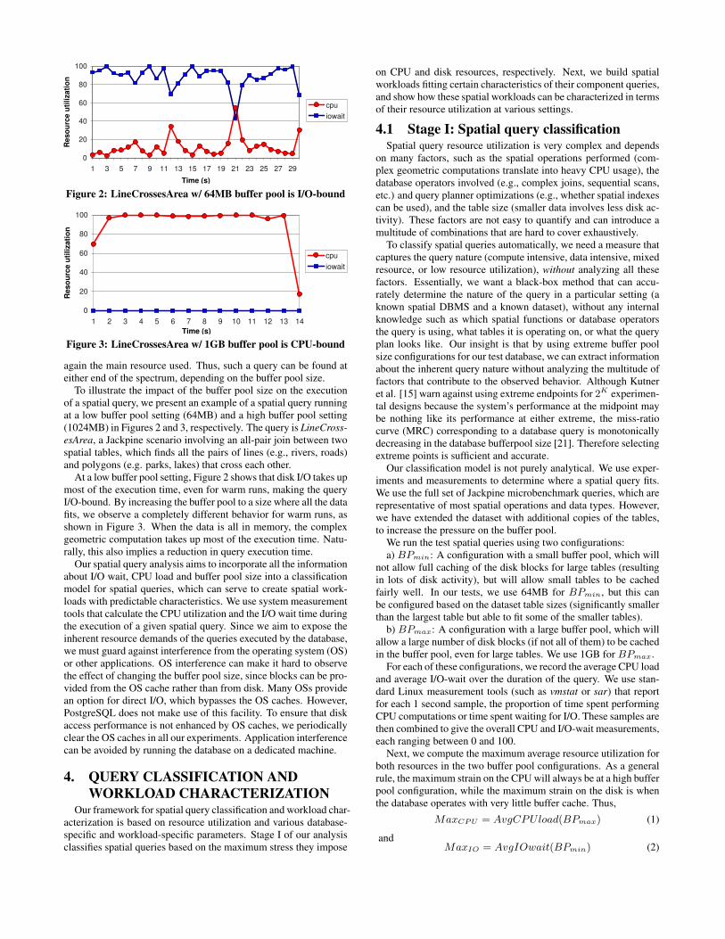
Figure 2: LineCrossesArea w/ 64MB buffer pool is I/O-bound

0

20

40

60

80

100

1 2 3 4 5 6 7 8 9 10 11 12 13 14

Time (s)

Reso

urc

e u

tili

zati

on

cpu

iowait

Figure 3: LineCrossesArea w/ 1GB buffer pool is CPU-bound

again the main resource used. Thus, such a query can be found ateither end of the spectrum, depending on the buffer pool size.

To illustrate the impact of the buffer pool size on the executionof a spatial query, we present an example of a spatial query runningat a low buffer pool setting (64MB) and a high buffer pool setting(1024MB) in Figures 2 and 3, respectively. The query is LineCross-esArea, a Jackpine scenario involving an all-pair join between twospatial tables, which finds all the pairs of lines (e.g., rivers, roads)and polygons (e.g. parks, lakes) that cross each other.

At a low buffer pool setting, Figure 2 shows that disk I/O takes upmost of the execution time, even for warm runs, making the queryI/O-bound. By increasing the buffer pool to a size where all the datafits, we observe a completely different behavior for warm runs, asshown in Figure 3. When the data is all in memory, the complexgeometric computation takes up most of the execution time. Natu-rally, this also implies a reduction in query execution time.

Our spatial query analysis aims to incorporate all the informationabout I/O wait, CPU load and buffer pool size into a classificationmodel for spatial queries, which can serve to create spatial work-loads with predictable characteristics. We use system measurementtools that calculate the CPU utilization and the I/O wait time duringthe execution of a given spatial query. Since we aim to expose theinherent resource demands of the queries executed by the database,we must guard against interference from the operating system (OS)or other applications. OS interference can make it hard to observethe effect of changing the buffer pool size, since blocks can be pro-vided from the OS cache rather than from disk. Many OSs providean option for direct I/O, which bypasses the OS caches. However,PostgreSQL does not make use of this facility. To ensure that diskaccess performance is not enhanced by OS caches, we periodicallyclear the OS caches in all our experiments. Application interferencecan be avoided by running the database on a dedicated machine.

4. QUERY CLASSIFICATION ANDWORKLOAD CHARACTERIZATION

Our framework for spatial query classification and workload char-acterization is based on resource utilization and various database-specific and workload-specific parameters. Stage I of our analysisclassifies spatial queries based on the maximum stress they impose

on CPU and disk resources, respectively. Next, we build spatialworkloads fitting certain characteristics of their component queries,and show how these spatial workloads can be characterized in termsof their resource utilization at various settings.

4.1 Stage I: Spatial query classificationSpatial query resource utilization is very complex and depends

on many factors, such as the spatial operations performed (com-plex geometric computations translate into heavy CPU usage), thedatabase operators involved (e.g., complex joins, sequential scans,etc.) and query planner optimizations (e.g., whether spatial indexescan be used), and the table size (smaller data involves less disk ac-tivity). These factors are not easy to quantify and can introduce amultitude of combinations that are hard to cover exhaustively.

To classify spatial queries automatically, we need a measure thatcaptures the query nature (compute intensive, data intensive, mixedresource, or low resource utilization), without analyzing all thesefactors. Essentially, we want a black-box method that can accu-rately determine the nature of the query in a particular setting (aknown spatial DBMS and a known dataset), without any internalknowledge such as which spatial functions or database operatorsthe query is using, what tables it is operating on, or what the queryplan looks like. Our insight is that by using extreme buffer poolsize configurations for our test database, we can extract informationabout the inherent query nature without analyzing the multitude offactors that contribute to the observed behavior. Although Kutneret al. [15] warn against using extreme endpoints for 2K experimen-tal designs because the system’s performance at the midpoint maybe nothing like its performance at either extreme, the miss-ratiocurve (MRC) corresponding to a database query is monotonicallydecreasing in the database bufferpool size [21]. Therefore selectingextreme points is sufficient and accurate.

Our classification model is not purely analytical. We use exper-iments and measurements to determine where a spatial query fits.We use the full set of Jackpine microbenchmark queries, which arerepresentative of most spatial operations and data types. However,we have extended the dataset with additional copies of the tables,to increase the pressure on the buffer pool.

We run the test spatial queries using two configurations:a) BPmin: A configuration with a small buffer pool, which will

not allow full caching of the disk blocks for large tables (resultingin lots of disk activity), but will allow small tables to be cachedfairly well. In our tests, we use 64MB for BPmin, but this canbe configured based on the dataset table sizes (significantly smallerthan the largest table but able to fit some of the smaller tables).

b) BPmax: A configuration with a large buffer pool, which willallow a large number of disk blocks (if not all of them) to be cachedin the buffer pool, even for large tables. We use 1GB for BPmax.

For each of these configurations, we record the average CPU loadand average I/O-wait over the duration of the query. We use stan-dard Linux measurement tools (such as vmstat or sar) that reportfor each 1 second sample, the proportion of time spent performingCPU computations or time spent waiting for I/O. These samples arethen combined to give the overall CPU and I/O-wait measurements,each ranging between 0 and 100.

Next, we compute the maximum average resource utilization forboth resources in the two buffer pool configurations. As a generalrule, the maximum strain on the CPU will always be at a high bufferpool configuration, while the maximum strain on the disk is whenthe database operates with very little buffer cache. Thus,

MaxCPU = AvgCPUload(BPmax) (1)

andMaxIO = AvgIOwait(BPmin) (2)

0

20

40

60

80

100

0 20 40 60 80 100

IO w

ait

1. AreaContainsArea 2. AreaDisjointArea3. AreaEqualsArea 4. AreaOverlapsArea6. AreaTouchesArea 7. AreaWithinArea9. BufferPolygon 25. PointEqualsPoint

11. DimensionPolygon 12. DistanceFromPoint13. EnvelopeLine 14. LargestAreaContainsPoint19. LineIntersectsLargestArea 24. LongestLine 26. PointIntersectsArea28. PointWithinArea 30. TotalLength

5. AreaOverlapsLargestArea10. ConvexHullPolygon23. LongestLineIntersectsArea

17. LineCrossesLine 8. BoundingBox15. LargestArea 29. TotalArea16. LineCrossesArea 18. LineIntersectsArea20. LineOverlapsArea 21. LineTouchesArea22. LineWithinArea 27. PointIntersectsLine

CPU load

Figure 4: Spatial query classification - color coding representsthe 4 query classes

These numbers represent the spatial query nature in terms ofdata-intensiveness (if MaxIO is high at BPmin, when disk activ-ity should be dominant), and computational intensity (if MaxCPU

is high at BPmax, when everything should theoretically fit in mem-ory). The difference between these two figures represents the vari-ation between the highest CPU-utilization and the highest I/O ac-tivity. This is a good indicator if a query has a more computationalnature (e.g, performing complex spatial operations on complex spa-tial types), or if data fetching activity is predominant.

In Figure 4, we plot the values of MaxCPU and MaxIO foreach query on a two-dimensional scatterplot with the CPU utiliza-tion on the x-axis and the I/O-wait on the y-axis. Intuitively, thequeries located in the upper left corner of the resource space shownin Figure 4 are data-intensive, since they have high I/O-wait timesbut do not saturate the CPU even at BPmax. Similarly, we can seethat the queries from the lower right corner are compute-intensive,since the I/O-wait is never a large factor, even at BPmin. Thequeries in the upper right corner are of a mixed nature, dependingon the buffer pool size, while the queries close to the lower leftcorner utilize few resources (low computation, few data accesses).

From this plot we can see that spatial queries differ widely interms of their maximum resource demand, with some being com-pute intensive while others are inherently data intensive. Based onthese observations, we can determine the query classes by splittingthe resource usage domain using a set of delimiting line segments:

y = x− a (3)

y = x+ b (4)

y = −x+ c (5)

In our work, we determined empirically that a = b = 40 and c =120 work well as the thresholds. With these equations, the resourceusage space is divided as shown by the colored regions in Figure 4.Using equations (3) and (4), we can determine the nature of a givenquery point Q(x,y):i. if x− y >= a%⇒ Query is compute-intensive (red region)ii. if x− y <= −b%⇒ Query is data-intensive (blue region)iii. if −b% < x − y < a% ⇒ Query is mixed (orange+purpleregions)

Category iii) is further split using equation (5):iii.a) if y + x < c%⇒ low resource utilization (orange region)iii.b) if y + x >= c%⇒ mixed resource usage (purple region)

Mixed usage queries arise either because varying the buffer poolsize migrates the query from the data-intensive end of the spectrumto the compute-intensive end, or simply because the query is usingboth resources in roughly equal proportions.

The visual representation in Figure 4 shows that this approachgroups queries into 4 classes: compute-intensive (class C), data-

0

20

40

60

80

100

0 20 40 60 80 100

CPU load

IO w

ait





(a) BPmin

0

20

40

60

80

100

0 20 40 60 80 100CPU load

IO w

ait





(b) BPmax

Figure 5: Mixed queries migrate from a data-intensive state atBPmin to a high computation region at BPmax

intensive (class D), mixed resource (class M1) and low resourceutilization (class M2). The legend lists the queries in each category.

Although the use of delimiting line segments works well for thisset of experiments, the empirical choice of thresholds is unsatisfac-tory. As a result, we use the intuition behind the different segmentsto construct a k-means clustering model.

4.1.1 Clustering-based classification modelWe implemented a clustering method which places the queries

into 4 clusters (corresponding to the 4 categories mentioned above).We use a k-means algorithm with 4 centroids and Euclidean dis-tance measure. The centroids are artificial points in the resourcespace, representing the "average location" of a particular cluster.The 4 centroids are placed initially at (90,10), (10,90), (90,90) and(10,10), corresponding to compute-intensive tasks, data-intensivetasks, mixed-resource tasks and low-resource tasks respectively.

The algorithm computes the distances from each point to eachof the centroids, then marks each point as belonging to the clusterwhose centroid is closest. Once the points are grouped into clusters,the centroids are recomputed by averaging the coordinates for eachof the points in the cluster. The process repeats until the centroidsstabilize (they remain the same after two successive iterations).

The query classes represented by the clusters are identical to theones obtained using the delimiting lines, further supporting that weaccurately capture the query nature and produce a correct classifi-cation. Figure 4 lists the queries contained in each cluster.

4.1.2 DiscussionWe observe that mixed resource queries (class M1) come in two

forms. The first type consists of queries that use roughly equalexecution time to perform computations and to fetch data blocks.Based on our experiments, this type is rare; only one example canbe found in Jackpine, namely the LineCrossesLine query. This sce-nario was limited to return 5 records, since it was the longest run-ning query (an all pair join between two 6-million record tables,representing all the intersections between line shapes such as roads

and rivers). When a data-intensive query such as LineCrossesLineonly has to fetch a limited amount of data, the computation be-comes significant and thus the query is evenly balanced in terms ofcomputation and time spent accessing data.

The second type consists of queries that are at opposite ends ofthe spectrum depending on the buffer pool size. In Figures 5(a)and 5(b) we illustrate how mixed-nature queries (class M1, markedwith purple triangles in the figures) queries migrate from I/O-boundat a low buffer pool size to CPU-bound at a high buffer pool size.

It is important to note that the query classification does not tellus whether a query is I/O-bound or CPU-bound. Instead, the classgives us insight into how the query will behave in different con-figurations. Figure 5 shows the behavior at the two extreme bufferpool configurations, illustrating how the behavior changes for thedifferent query classes. This figure motivates one additional refine-ment to our classification. We observe that data-intensive queries(class D) come in two types. The first type (class D1) is I/O-boundwith a low buffer pool and low-CPU with a high buffer pool, whilethe second category (class D2) stays I/O-bound, even with a signif-icantly large (yet reasonable size) buffer pool. Class D1 containsqueries that cannot saturate the CPU even when all the data fits inthe buffer cache; it accounts for most of the data-intensive queriesfrom Jackpine. The queries that are included in class D2 are En-velopeLine, LongestLine and TotalLength.

In summary, the Stage I analysis groups spatial queries into 5major classes: compute-intensive (class C), data-intensive (classesD1 and D2), and mixed (classes M1 and M2). The next stage se-lects queries of a given class to create spatial workloads with aknown homogeneous nature.

4.2 Stage II: Spatial workloadcharacterization

In the second stage of our framework, our goal is to characterizespatial workloads as we vary database-specific parameters (mostsignificantly, the buffer pool size) and workload-specific parame-ters (e.g., the query density in the workload mix). Given the clas-sification of all the test queries in Stage I, we aim to determine ifa workload comprised of queries from a given class is CPU-bound,I/O-bound or a mix of both, in different configurations.

4.2.1 Jackpine workload supportTo test and analyze spatial workloads, we extend the Jackpine

benchmark to support fully concurrent heterogeneous query execu-tion. Jackpine only had limited support for concurrent query execu-tion. Specifically, it could launch multiple threads within the samescenario to execute multiple instances of the same query. However,to provide realistic workloads containing any combination of dis-tinct spatial queries running concurrently we require more flexiblesupport for concurrent scenarios.

We use the modified Jackpine benchmark to drive custom work-loads for the Stage II analysis. Jackpine now launches a workload,based on a configuration file that contains the descriptions of thescenarios to be executed concurrently. Each scenario in turn hasits own configuration file, containing the description of the spatialscenario class, and a set of parameters. One of these parametersspecifies how many instances of that query should be included inthe workload mix. Consequently, a workload can contain multipledistinct scenarios (corresponding to distinct spatial queries), andeach scenario can have multiple instances of the same query. All ofthese queries are run concurrently.

To isolate the performance of the database from that of the bench-mark driver, we run Jackpine on a separate machine; queries areissued to the database using JDBC connections.

4.2.2 Workload characterization via resource usageOur goal is to characterize spatial workloads by varying several

factors that can have a significant impact on the resource usage ofa given workload. As we have seen, one critical factor is the bufferpool size, which determines whether the data and index blocksneeded by a workload can fit entirely in memory, thus eliminatingexpensive disk accesses. Based on the buffer pool size, a workloadcan be characterized as either I/O-bound, mixed, or CPU-bound. Ifall needed data fits in the buffer pool, we can determine whetherthe CPU usage is high or low without the interference of fetchingdata from disk. In contrast, some queries perform sequential scanson large tables which will not fit into even a large buffer pool.

Another important parameter is query density. In generic databaseworkloads, there are a finite number of tables in a dataset, but alarge number of query types and combinations. This leads us to thesafe assumption that the number of queries in the average workloadmix is much larger than the number of tables used. In turn, thismeans that many queries will be accessing the same tables concur-rently, which would enable sharing of buffer pool pages. Based onthe density of the queries in the workload mix, this sharing effectcan have a significant impact on the workload nature as it attractsworkloads towards the CPU-intensive end of the spectrum. Ba-sically, workloads that are already CPU-bound will be even moredominantly CPU-bound, while for I/O-bound workloads the diskactivity dimension will become less predominant.

Because disk accesses are very expensive, some queries are I/O-bound even though they perform heavy computations. However,when the query density is high, a large number of I/O-bound querieswill be accessing the same tables and will inevitably share pages inthe buffer pool. The result is a higher hit ratio, which in turn re-duces the amount of disk accesses. This buffer pool sharing couldresult in a CPU-bound workload comprised of individually I/O-bound queries, given that the CPU-work cycles for each individualquery in the workload cannot be shared.

We design 5 types of workloads corresponding to the query classesdescribed in Section 4.1. The workloads are homogeneous in thequery class types, but contain a mix of distinct queries. Thus, work-loads are composed of either C, D1, D2, M1 or M2-class queries.The buffer pool size and query density are the testing parameters;by varying them, the workload nature can change dramatically forD-class and M-class workloads, but not for the C-class, as we willshow. We use 2 buffer pool settings (low/high) corresponding toBPmin and BPmax configurations. We use 3 query density set-tings: low, medium and high. With the low setting, the workloadcontains a single query of the respective query class. A mediumsetting includes a mix of 6 queries, while a high setting contains 30concurrent queries. To better show the trends, we chose one moremix (of 12 queries) for the medium setting and two extra mixes (24and 48 concurrent queries) for the high setting. The basic charac-terization can be obtained with just the initial 3 mixes, however.

As in Stage I, CPU load and I/O activity measurements are takenat 1 second intervals and averaged over the execution time of theworkload. The average CPU load and the average I/O-wait rep-resent the percentage of time executing CPU instructions and thepercentage of time fetching either data or index pages from disk.

We use a visual representation of the resource usage for theseworkloads in a two-dimensional space, where the coordinates arequery density (x-axis) and buffer pool size (y-axis). We draw a linebetween the low and high buffer pool settings, corresponding to thesize where the miss-ratio curve (MRC) drops to zero buffer poolmisses. This BP-cutoff will occur at different buffer pool sizes fordifferent queries. We do not determine the actual cutoff, we merelyobserve that behavior will be different above and below this line.

Low

BP-cutoff

High

Low Medium High

Bu

ffe

r p

oo

l siz

e

Query density

IO m

ixed C

PU

bound b

ound

(a) Class C workload

Low

BP-cutoff

High

Low Medium High

Bu

ffe

r p

oo

l siz

e

Query density

IO m

ixed C

PU

bound b

ound

(b) Class D1 workload

Low

BP-cutoff

High

Low Medium High

Bu

ffe

r p

oo

l siz

e

Query density

IO m

ixed C

PU

bound b

ound

(c) Class D2 workload

Low

BP-cutoff

High

Low Medium High

Bu

ffe

r p

oo

l siz

e

Query density

IO m

ixed C

PU

bound b

ound

(d) Class M1 workload

Low

BP-cutoff

High

Low Medium High

Bu

ffe

r p

oo

l siz

e

Query density

IO m

ixed C

PU

bound b

ound

(e) Class M2 workload

Figure 6: Resource usage maps. Color coding is used for resource usage: CPU computations are shown in shades of red (darkermeans more computation), I/O activity is in blue nuances, while mixed is in shades of purple (depending on the mix of CPU and I/O).

The resource utilization is color-coded (similar to heat maps) intoresource usage maps for each of the test workloads.

Figure 6 (a)-(e) shows the resource usage maps for each of theworkload types. Our experiments show that the compute-intensiveclass C queries (Figure 6(a)) are CPU-bound regardless of bufferpool size or query density. This is an expected result, since increas-ing the buffer pool size and/or query density can only increase thedemand on the CPU. However, for data-intensive and mixed queryclasses, the workload categorization gets considerably more com-plex, as the workloads can turn out to be either I/O-bound, mixedor even CPU-bound, in different configurations. In the followingtext, we use the abbreviation “QD” to refer to query density.

The D1 category is I/O-bound at a (low QD; low BP) configu-ration, and low CPU usage at a (low QD; high BP) setting. Thisshows that each of the queries in this category individually ex-hibit this behavior, as expected. As query density increases, at alow BP setting the concurrent queries start sharing pages in thebuffer pool and therefore the workload migrates towards a mixedresource utilization (for QD=high). With a high BP setting and in-creasingly higher QD, the workload performs more computationexerting more pressure on the CPU and (predictably) becomingCPU-bound. The D2 category exhibits a trend of slowly transition-ing from I/O-bound towards mixed and CPU-bound as query den-sity increases. The M1 category is similar to D1, except that hav-ing more computation speeds up the transition from an I/O boundto a CPU-bound behavior at a low buffer pool setting and leadsto consistently CPU-bound behavior at a high buffer pool setting.The M2 category exhibits a low resource utilization behavior fora low query density, but as the number of queries in the workloadmix increases, the workload behavior changes. By adding morequeries (which use more data tables), the workload first becomesI/O-bound at a medium QD setting, only to migrate towards CPU-bound as more queries are added at a high QD setting (with thenumber of data tables staying the same). With a high buffer poolsetting, an M2 workload transitions from low-CPU usage to CPU-bound behavior as QD increases.

As a general observation, once a workload becomes CPU-boundincreasing the query density can only leave the workload CPU-bound, if the number of data tables in the dataset stays the same.If each query would operate on its own copy of the data table, thesituation would be different. However, as noted earlier, we makethe reasonable assumption that the number of queries in a spatialworkload far exceeds the number of tables in the dataset.

These resource usage maps provide valuable information on the

behavior of any spatial workload. Database administrators anddatabase users can use these maps to understand which resourcesare heavily utilized and what to expect with changes in the work-load query density. Given a buffer pool size and the workload mix,these categories can pinpoint the nature of the workload (CPU-bound, I/O-bound, mixed etc.). Furthermore, this helps determinewhere to focus performance upgrades to deal with increased pres-sure on a given resource.

5. APPLICATION TO NEW WORKLOADSTo demonstrate that our characterization provides useful guid-

ance on the behavior of a target workload, we test realistic spatialworkloads drawn from the Jackpine macrobenchmark scenarios.We show that the classifications obtained by our framework ac-curately predict the behavior of these workloads at different bufferpool size and query density settings. Further, we show how thischaracterization can serve to guide resource upgrades.

5.1 Experimental setupFor the query classification and workload characterization stages,

we use an Intel Core 2 Duo E7500 at 2.93GHz, 3MB cache, and4GB RAM, running Ubuntu Linux 10.04, 64-bit with 2.6.26 kernelversion, and PostgreSQL 8.4.4 with PostGIS spatial extension. Allthe results in the previous sections were obtained on this machine.

When running on a machine with multiple cores, Linux measure-ment tools average out the CPU load and I/O wait time among thecores, whether active or not. To obtain correct measurements, wedisabled one core when running the workloads. On Linux, this canbe done dynamically by writing “0” to a system file (e.g. “echo0 > /sys/devices/system/cpu/cpu1/online”).

5.2 Classifying realistic workloadsTo test the accuracy of our categorization framework on real-

world spatial applications, we use all but one of the Jackpine work-loads from the macrobenchmark suite (Map Browsing, Land Infor-mation Management, Flood Risk Analysis, Toxic Spill and ReverseGeocoding). We omitted the Geocoding scenario, since it does notuse spatial shapes, just latitude-longitude coordinates.

In Stage I, each macrobenchmark scenario is classified into data-intensive, compute-intensive, or mixed (as well as the appropri-ate subcategories). In Stage II, we select two interesting scenariosin terms of resource usage (MapBrowsing and Land InformationManagement, which are also among the most widely-used spatialapplications) to demonstrate that the resource usage maps for their

0

20

40

60

80

100

0 20 40 60 80 100CPU load

IOw

ait

Map Browsing

Land Info Management

Flood Risk

Toxic Spill

Reverse Geocoding

Figure 7: Classifying realistic application workloads.

respective classes can be used to accurately predict the resource-boundness of the workloads in a wide range of configurations.

The Map Browsing and Land Information Management scenar-ios are described in detail in [19]. For completeness, we provide ashort description for each of them here.

Map Browsing. Searching for locations of interest by keywordsand viewing the results on a map is a popular use of online map-ping applications. For example, a tourist visiting a new city maylook for nearby airport, hotels, restaurants, and popular sites. TheMap Browsing scenario models such use cases by first performinga search query for a place of interest. Then a series of 5 queriesare executed that fetch the spatial objects inside a bounding boxcentered around the found location of interest. The sequence ofsearching for a nearby place of interest and 5 map display queriesare repeated a number of times to reflect typical browsing behavior.

Land Information Management. Land information managementis vital to the maintenance of property ownership and the enforce-ment of land use regulations. Digital land information managementsystems, where parcels of property are stored as shapes in a geospa-tial database, are a valuable tool to many local governments. Theland information data set used in Jackpine was obtained from theCity of Austin GIS data sets. Several land use related queries areexecuted in sequence during the scenario.

We first show how the Stage I process can be used to classify thespatial workloads into one of the 5 categories. Each of the macroscenarios are individually run and classified using the delimitingline segments (clustering with the other queries yields the sameclassification). The results are shown in Figure 7. Map Brows-ing has a highly data-intensive nature, belonging in the D2 class,whereas Land Information Management is of a mixed nature, fittinginto class M1. The Flood Risk analysis is CPU-bound (C-class) andthus is not as interesting to study since the resource usage map isCPU-bound at all settings. Toxic Spill is similar to Map Browsingand fits into the D2 category, while Reverse Geocoding matches theD1 class. Note that only two measurements are needed to obtain theclassification for a given workload.

Based on this classification, the resource maps from Figure 6 inSection 4.2 can be applied to predict how these workloads change atdifferent settings. Due to space constraints, we selected for analysisthe Map Browsing and Land Information Management scenarios,as they are representative of the most interesting query classes (D2and M1), which provide a wide range of resource usage variation.

To demonstrate that the resource usage maps for the correspond-ing classes (obtained with the homogeneous workloads) can accu-rately predict workload behavior, we pass the workloads throughStage II and measure resource usage at various buffer pool andquery density settings. The resulting resource usage maps are plot-ted in Figures 8(a) and 8(b). As can be seen from these maps, the

Map Browsing workload clearly matches the behavior of the D2class at different buffer pool sizes and query densities, while LandInformation Management matches the behavior of the M1 class.

We conclude that employing the resource usage maps for work-loads of a particular nature (i.e., class) can accurately predict theirbehavior in various configurations.

Note that our goal is not to predict exact performance under agiven configuration, but rather to capture the resource usage trendof an application as database-specific and workload-specific param-eters change. Consequently, the buffer pool size and query den-sity settings must not be taken as absolute values, but rather asa means to capture the workload behavior trend. We argue thatthe methodology behind our framework creates resource utilizationmaps which are widely-applicable in this respect. For example,in production databases, the dataset will probably be much largerthan our dataset, but so will the buffer pool size settings. Even ifthe dataset and buffer pool size increases are not proportional, theperformance trend will still be captured in the resource utilizationmaps. Our ultimate goal is to provide clues to DBAs in capac-ity planning decisions, by using these maps as a predictor of howworkload changes can impact the performance trends.

6. VARYING DBMS AND DATASETTo validate the classification methodology, we apply it to a sec-

ond database, as well as to a much larger dataset.

6.1 InformixDifferent DBMSs implement spatial processing in different ways,

and not all are OGC-compliant. For example, MySQL does not per-form the refinement step. Other DBMSs use different implementa-tions of the spatial functions and/or perform various optimizationsfor the relational operators (e.g., sequential and index scans, joinsetc). Consequently, the results of our framework on one DBMScannot be blindly applied across all DBMSs. The framework mayplace the same query executed on different DBMSs in different cat-egories, simply because different implementations of spatial oper-ators across DBMSs, as well varying database internals (such asbuffer pool management and query optimizations) may entail dif-ferent resource utilization.

However, an important aspect of our analysis is to determine ifthe query classification method can be used for any DBMS. Thus,we perform a validation with a different DBMS, by applying thesame strategy to Informix, a closed-source commercial DBMS. Infigure 9 we show the resource usage of the same set of spatialqueries, executed through the Informix engine and its spatial ex-tension. Since Informix does not support the ST_Buffer spatialfunction, we exclude one query involving this functionality.

Overall, the classification is quite similar to PostgreSQL in termsof the resource usage of different queries, with the exception thatInformix seems to exhibit better I/O performance for some of thequeries, such as TotalLength, TotalArea, LongestLine, LargestAreaand LineCrossesLine. As a result, these queries get classified in adifferent category than for PostgreSQL.

Since Informix is closed-source, we could not confirm with thesource code the exact reason for better I/O performance, but wedid notice that all the aforementioned queries include a sequentialscan of a large table (edges_merge and areawater_merge) as partof the query plan. As a result, we speculate that Informix is betteroptimized for sequential scans of large data tables. Additionally,since Informix stores data on disk as contiguous large blocks called“dbspaces” and “sbspaces” (for spatial data), we speculate that theprefetcher may also contribute to the better I/O performance.

Even without having information about the query plans, inter-

Low

BP-cutoff

High

Low Medium High

Buffer

pool siz

e

Query density

IO m

ixed C

PU

bound b

ound

(a) Map Browsing

Low

BP-cutoff

High

Low Medium High

Buffer

pool siz

e

Query density

IO m

ixed C

PU

bound b

ound

(b) Land Info Management

Figure 8: Resource usage maps for realistic workloads

0

20

40

60

80

100

0 20 40 60 80 100

IO w

ait

CPU load

1. AreaContainsArea 3. AreaEqualsArea 6. AreaTouchesArea15. LargestArea24. LongestLine29. TotalArea

2. AreaDisjointArea 4. AreaOverlapsArea 7. AreaWithinArea17. LineCrossesLine25. PointEqualsPoint30. TotalLength

11. DimensionPolygon12. DistanceFromPoint14. LargestAreaContainsPoint19. LineIntersectsLargestArea26. PointIntersectsArea

13. EnvelopeLine

28. PointWithinArea

8. BoundingBox18. LineIntersectsArea21. LineTouchesArea27. PointIntersectsLine

16. LineCrossesArea20. LineOverlapsArea 22. LineWithinArea


Figure 9: Classification for Informix.

0

20

40

60

80

100

0 20 40 60 80 100

IO w

ait

CPU load

1. AreaContainsArea 3. AreaEqualsArea 6. AreaTouchesArea 9. BufferPolygon26. PointIntersectsArea

2. AreaDisjointArea 4. AreaOverlapsArea 7. AreaWithinArea25. PointEqualsPoint28. PointWithinArea

11. DimensionPolygon12. DistanceFromPoint14. LargestAreaContainsPoint19. LineIntersectsLargestArea24. LongestLine

13. EnvelopeLine

30. TotalLength

8. BoundingBox16. LineCrossesArea18. LineIntersectsArea21. LineTouchesArea27. PointIntersectsLine

15. LargestArea17. LineCrossesLine20. LineOverlapsArea 22. LineWithinArea29. TotalArea


Figure 10: Classification with larger dataset (contiguous US).

nal query processing optimizations, data layout on disk, and otherdatabase internals of Informix, the classification framework wasable to accurately place these spatial queries according to their re-source utilization. Moreover, although Informix seems to performmore computation and do slightly more I/O for some of the queriesclassified as low utilization for PostgreSQL (marked with orangecircles), the classification model is still able to distinguish theserelatively short-running queries from the data-intensive cluster ofqueries and mark them as low utilization for Informix as well.

6.2 Dataset scalabilityAn important aspect of our classification is that it can be per-

formed for any size spatial dataset. To illustrate this, we validatedour approach against a much larger dataset. We used TIGER datafor the entire contiguous US (48 states, instead of just the state ofTexas), which amounted to roughly 32GB. We adjusted the bufferpool sizes in line with our concept of testing at extreme low andhigh settings to accurately determine the nature of a spatial query(computationally-intensive, data intensive, or mixed).

Figure 10 shows that the overall trend for spatial queries on theUS dataset is towards more computation than for the Texas dataset,for all queries analyzed, with I/O making slightly less of an im-

pact. In most cases, the spatial queries remain in the same classesas before, with two surprising exceptions. Two of the queries thatwere previously classified as data-intensive (PointIntersectsAreaand PointWithinArea) on the Texas dataset have now migrated to-wards computationally intensive. The trend towards more com-putation is explicable since in the case of complex queries moreobjects lead to more complex geometry calculations, and computa-tions on larger data end up outweighing the increased disk activity.

The queries labelled low-utilization with the Texas dataset re-main low-utilization on the US dataset as well, and are classifiedas such. However, there is a slight trend towards either the databecoming more dominant (e.g., LongestLineIntersectsArea), or thecomputation (e.g., ConvexHullPolygon).

Overall, the experiments with a larger dataset confirm that ourclassification method exposes the inherent nature of spatial queries.However, these results must be considered in the context of thespatial dataset, since the inherent features of a large dataset maysway some of the spatial queries towards a different class.

7. RELATED WORKA survey of the early research on workload characterization can

be found in [6]. Various research projects attempted to characterizedatabase workloads using different approaches. Yu et al. [26] pre-sented a method based on the analysis of the structure of SQL state-ments, the behavior of transactions, and the composition of tablesand views. Several projects used clustering techniques to groupworkloads based on similarity metrics, such as response time. Someof the early works that used clustering to classify workloads aresummarized in [18]. Wasserman et al. [24] described a databaseworkload classification approach based on system resource attributes.A few studies focused on characterizing the database access pat-terns. For instance, in [8] the authors identified three types of ac-cess patterns. Additionally, they addressed the issue of characteriz-ing the random access pattern and predicting its buffer hit probabil-ities with various buffer pool configuration. Sapia [20] studied thehigh level access patterns of OLAP (Online Analytical Processing)queries with an eye towards improved caching techniques. Usingtrace-driven simulations Hsu et al. [12] systematically examinedthe properties of production workloads in relation to the TPC-C andTPC-D workloads and concluded that the production workloads aredynamic and time-varying in their characteristics. Oh and Lee [16]conducted a study to analyze how changes in resource size impactresource usage and proposed a method to identify the resourceswith significant influence over system performance.

Other research projects investigated database workloads to studyhardware system behavior and performance issues in commercialapplications. Barroso et al. [3] examined the memory system be-havior of the OLTP and DSS workloads. In [14] the database per-formance on SMT processors was analysed, whereas, in [13] theauthors studied the effectiveness of several architectural features ofa multiprocessor SMP running commercial database workloads.

Previous database workload characterization research dealt withtraditional database workloads, such as those from the TPC suites.In contrast, we focus on spatial database workloads. An impor-tant aspect of our approach is the small number of profile runs thatare required per workload to produce the resource usage map, incontrast to other approaches such as [16] that require many moreprofile runs to characterize resource usage.

Databases are not unique in being the subject of workload char-acterization. Arlitt [2] characterized user sessions from web pageaccesses. Eeckhout et al. focused on Java workload characteri-zation [9]. Many other examples of workload characterization re-search can be found.

8. CONCLUSIONSSpatial workloads are different from previously studied database

workloads. Using microprocessor performance events, we showthat spatial queries stress the CPU in different ways from decisionsupport queries in TPC-H. This may point to opportunities for im-proving the implementation of spatial operators.

We then introduce a two-stage framework for classifying spatialqueries based on their nature (compute-intensive, data-intensive ormixed) and characterizing spatial workloads based on resource uti-lization at various settings. Our approach is unique because weincorporate concurrent query interaction by varying query density.Thus, we capture the dynamic nature of the resource consumptionof spatial workloads with the change in query density and systemconfiguration parameters. Finally, we show how this frameworkcan characterize any spatial workload simulating real-world appli-cations. We also present a novel resource usage map that providesa concise, yet information-rich description of the workload behav-ior with various system configurations and load conditions. Thisserves as a tool for database administrators (DBAs) to use in de-termining which resources are heavily utilized and thus to performresource upgrades in a smart way.

We validate our methodology using a second DBMS and a sec-ond, much larger dataset. As future work, our goal is to apply thisprocess dynamically to detect changes in workloads online, therebysupporting dynamic provisioning.

9. ACKNOWLEDGMENTSWe would like to thank Ryan Johnson and the anonymous re-

viewers for their valuable feedback. We also thank Eric Logan forassistance with machine configurations. This research was sup-ported by an NSERC Discovery Grant. Suprio Ray is supported byan NSERC PGS-D scholarship.

10. REFERENCES[1] A. G. Ailamaki, D. J. Dewitt, M. D. Hill, and D. A. Wood.

DBMSs on a modern processor: Where does time go. In IntlConference on Very Large Data Bases, pages 266–277, 1999.

[2] M. Arlitt. Characterizing web user sessions. SigmetricsPerformance Evaluation Review, 28:50–63, 2000.

[3] L. A. Barroso, K. Gharachorloo, and E. Bugnion. Memorysystem characterization of commercial workloads. In IntlSymposium on Computer Architecture, pages 3–14, 1998.

[4] The Calibrator, a cache-memory and TLB calibration tool.http://homepages.cwi.nl/ manegold/Calibrator/.

[5] M. Calzarossa and L. Massari. Workload characterizationissues and methodologies. In Performance Evaluation:Origins and Directions, Lect. Notes Comput. Sci., 2000.

[6] M. Calzarossa and G. Serazzi. Workload characterization: asurvey. Proceedings of The IEEE, 81:1136–1150, 1993.

[7] City of Austin GIS Data Sets.ftp://ftp.ci.austin.tx.us/GIS-Data/Regional/coa_gis.html.

[8] A. Dan, P. S. Yu, and J. Chung. Characterization of databaseaccess pattern for analytic prediction of buffer hit probability.The VLDB Journal, 4:127–154, 1995.

[9] L. Eeckhout, A. Georges, and K. D. Bosschere. How Javaprograms interact with virtual machines at themicroarchitectural level. In Proc. of OOPSLA, pages169–186, 2003.

[10] S. Elnaffar. Towards workload-aware DBMSs: IdentifyingWorkload Type and Predicting its change. PhD thesis,Queen’s University, Canada, 2004.

[11] S. Elnaffar, P. Martin, and R. Horman. Automaticallyclassifying database workloads. In Intl Conference on Info.and Knowledge Management, pages 622–624, 2002.

[12] W. W. Hsu and A. J. Smith. Characteristics of productiondatabase workloads and the TPC benchmarks. IBM SystemsJournal, 40:781–802, 2001.

[13] K. Keeton, D. A. Patterson, Y. Q. He, R. C. Raphael, andW. E. Baker. Performance characterization of a QuadPentium Pro SMP using OLTP workloads. In Intl Symposiumon Computer Architecture, volume 26, pages 15–26, 1998.

[14] J. L. Lo, L. A. Barroso, S. J. Eggers, K. Gharachorloo, H. M.Levy, and S. S. Parekh. An analysis of database workloadperformance on simultaneous multithreaded processors. InIntl Symposium on Computer Arch., pages 39–50, 1998.

[15] J. N. Michael H. Kutner, Christopher J. Nachtsheim andW. Li. Applied Linear Statistical Models (5th edition).McGraw-Hill International, New York, 2005.

[16] J. S. Oh and S. H. Lee. Resource selection for autonomicdatabase tuning. In ICDE Workshops, 2005.

[17] Open Geospatial Consortium.http://www.opengeospatial.org/ogc.

[18] K. E. E. Raatikainen. Cluster analysis and workloadclassification. Sigmetrics Performance Evaluation Review,20:24–30, 1993.

[19] S. Ray, B. Simion, and A. D. Brown. Jackpine: A benchmarkto evaluate spatial database performance. In Intl. Conf. onData Engineering, April 2011.

[20] C. Sapia. PROMISE: Predicting query behavior to enablepredictive caching strategies for OLAP systems. In DataWarehousing and Knowledge Disc., pages 224–233, 2000.

[21] G. Soundararajan, D. Lupei, S. Ghanbari, A. D. Popescu,J. Chen, and C. Amza. Dynamic resource allocation fordatabase servers running on virtual storage. In Conference onFile and Storage Technologies, pages 71–84, 2009.

[22] TIGER R©, TIGER/Line R© and TIGER R©-Related Products.http://www.census.gov/geo/www/tiger.

[23] The Transaction Processing Performance Council.http://www.tpc.org.

[24] T. J. Wasserman, P. Martin, D. B. Skillicorn, and H. Rizvi.Developing a characterization of business intelligenceworkloads for sizing new database systems. In Intl Workshopon Data Warehousing and OLAP, pages 7–13, 2004.

[25] G. Weikum, A. Moenkeberg, C. Hasse, and P. Zabback.Self-tuning database technology and information services:from wishful thinking to viable engineering. In IntlConference on Very Large Data Bases, pages 20–31, 2002.

[26] P. S. Yu, M. Chen, H. Heiss, and S. Lee. On workloadcharacterization of relational database environments. IEEETransactions on Software Engineering, 18:347–355, 1992.

surveying the landscape: an in-depth analysis of spatial

Documents