survey of deployment algorithms in wireless sensor
TRANSCRIPT
HAL Id: hal-01095749https://hal.inria.fr/hal-01095749
Submitted on 16 Dec 2014
HAL is a multi-disciplinary open accessarchive for the deposit and dissemination of sci-entific research documents, whether they are pub-lished or not. The documents may come fromteaching and research institutions in France orabroad, or from public or private research centers.
L’archive ouverte pluridisciplinaire HAL, estdestinée au dépôt et à la diffusion de documentsscientifiques de niveau recherche, publiés ou non,émanant des établissements d’enseignement et derecherche français ou étrangers, des laboratoirespublics ou privés.
Survey of Deployment Algorithms in Wireless SensorNetworks: Coverage and Connectivity Issues and
ChallengesInes Khoufi, Pascale Minet, Anis Laouiti, Saoucene Mahfoudh
To cite this version:Ines Khoufi, Pascale Minet, Anis Laouiti, Saoucene Mahfoudh. Survey of Deployment Algorithms inWireless Sensor Networks: Coverage and Connectivity Issues and Challenges. International journal ofautonomous and adaptive communications systems, Inderscience Publishers, 2017, 10 (4), pp.341-390.�10.1504/IJAACS.2017.10009671�. �hal-01095749�
Int. J. Autonomous and Adaptive Communications Systems, Vol. x, No. x, 20xx 1
Survey of Deployment Algorithms in Wireless SensorNetworks: Coverage and Connectivity Issues andChallenges
Ines KhoufiINRIA, Rocquencourt,78153 Le Chesnay Cedex, France,Email: [email protected]
Pascale MinetINRIA, Rocquencourt,78153 Le Chesnay Cedex, France,[email protected]
Anis LaouitiTELECOM SudParis,CNRS Samovar UMR 5157,91011 Evry Cedex, France,Email: [email protected]
Saoucene MahfoudhINRIA, Rocquencourt,78153 Le Chesnay Cedex, France,[email protected]
Abstract: Wireless Sensor Networks (WSNs) have many fields of application, including industrial,environmental, military, health and home domains. Monitoring a given zone is one of the maingoals of this technology. This consists in deploying sensor nodes in order to detect any eventoccurring in the zone of interest considered and report this event to the sink. The monitoring taskcan vary depending on the application domain concerned. In the industrial domain, the fast andeasy deployment of wireless sensor nodes allows a better monitoring of the area of interest intemporary worksites. This deployment must be able to cope with obstacles and be energy efficientin order to maximize the network lifetime. If the deployment is made after a disaster, it will operatein an unfriendly environment that is discovered dynamically. We present a survey that focuses ontwo major issues in WSNs: coverage and connectivity. We motivate our study by giving differentuse cases corresponding to different coverage, connectivity, latency and robustness requirements ofthe applications considered. We present a general and detailed analysis of deployment problems,while highlighting the impacting factors, the common assumptions and models adopted in theliterature, as well as performance criteria for evaluation purposes. Different deployment algorithmsfor area, barrier, and points of interest are studied and classified according to their characteristics andproperties. Several recapitulative tables illustrate and summarize our study. The designer in charge ofsetting up such a network will find some useful recommendations, as well as some pitfalls to avoid.Before concluding, we look at current trends and discuss some open issues.
Keywords: area coverage, barrier coverage, coverage, deployment algorithms, full connectivity, grid,intermittent connectivity, node activity scheduling, point of interest coverage, sensor deployment,virtual forces, wireless sensors, WSN
Biographical notes: Ines Khoufi received her Computer Science Engineering and Master degreesfrom the National College of Computer Science (ENSI) in 2010 and 2011 respectively. Currently,she is a Ph.D. student in HIPERCOM2 research team at Inria. Her current research interest is onwireless sensor networks deployment and progressive discovery of an unfriendly environment.
Pascale MINET works at the Inria research center of Rocquencourt, near Versailles. She is head of theHIPERCOM (High Performance Communication) team. She got her qualification in advising PhDstudents in 1998 from the University of Versailles. Previously she got her PhD diploma in ComputerScience, the University of Toulouse and her Engineer diploma in Computer Science in 1980 from
Copyright © 20xx Inderscience Enterprises Ltd.

2 I. Khoufi, P. Minet, A. Laouiti and S. Mahfoudh
ENSEEIHT (Engineering school of Toulouse). Her research topics relate to wireless sensor networksand mobile ad hoc networks and more particularly energy efficiency, routing, node activityscheduling, multichannel communication, redeployment and quality of service in these networks.She is co-author of the OLSR routing protocol standardized at IETF.
Anis Laouiti is an associate professor at Telecom SudParis since 2006. Before, he did his Phdresearch work and worked as a research engineer within Hipercom team at Inria-Rocquencourtwhere he participated to the OLSR routing protocol design (RFC3626). His research covers differentaspects in wireless ad hoc and mesh networks including protocol design, performance evaluationand implementation testbed.
Saoucene MAHFOUDH received her Computer Science Engineering degree from ENSI in 2005and her Master degree from the University of Paris 6 in 2006. She obtained her Ph D diploma in2010 from the University of Paris 6. Her research topics deal with energy efficiency, cross-layering,routing and redeployment in wireless sensor networks. After a post-doctoral fellow at Inria, she hasbeen working at King AbdelAziz University since 2013.
1 Introduction
With the emergence of the Internet of Things (IoT),several billion electronic devices and machines will beable to be connected to one another via the Internet.The devices will be able to communicate without theintervention of humans. Such communication is calledMachine-to-Machine communication, denoted M2M, andmobile wireless technology is an ideal technology to supportM2M communication. These emerging technologies basedon wireless communication can be autonomous and copewith changes without any human help. As an example, thefast and easy deployment of mobile wireless sensors in atemporary worksite is very useful for maintenance purposesand quality insurance. As these wireless sensor nodes arebattery equipped, the deployment should be energy efficientin order to maximize network lifetime. Sensors can also beused for damage assessment after a disaster, when the networkinfrastructure has been damaged. In this case, the WirelessSensor Network (WSN) operates in an unfriendly environmentthat can only be discovered progressively. However, somemajor challenges need to be tackled, such as:
• How to deal with the large volume of data produced.Collecting and exploiting these large data flows iscommonly known as big data transfer and processing.
• How to organize communication. Communicatingobjects will exist everywhere. They are generally usedto monitor a phenomenon. This phenomenon can bemonitored by a single object (e.g. the temperature ofcoffee in a mug) or require collaboration between severalobjects, which are usually deployed in a predefined area.In the latter case, these objects need to communicate andorganize themselves in the form of a network. That is thefocus of this paper.
Depending on the size of the entity (area, barrier or pointof interest) monitored, a multi-hop network may need to bedeployed to enable the monitoring of this area as well asthe delivery of the collected data. To meet the applicationrequirements, the deployment of these communicating objects(e.g. sensor nodes) must ensure coverage and connectivityproperties. Roughly speaking, coverage refers to the abilityto detect events occurring in the entity monitored (e.g. area,barrier, point of interest) whereas connectivity refers to theability to report this event to the sink.
1.1 Motivation
There are several types of coverage and connectivity problemsin WSNs.
With regard to the coverage of the entity monitoredwe distinguish between area, barrier and point of interestcoverage. Furthermore, the coverage can be full (i.e. anypoint of the entity is covered) or partial, depending on theapplication requirements. If the coverage is full, any point canbe monitored by a single sensor node (i.e. simple coverage) orby several sensor nodes (i.e. multiple coverage), depending onthe degree of robustness required. If the application requiresshort delays to detect an event, any point must be permanentlycovered. In other cases, any point is temporarily covered.
With regard to connectivity, if the application requiresshort delays to report the event detected to the sink, permanentconnectivity is needed. Otherwise, intermittent connectivityis sufficient. An example is given by a mobile robot collectingdata from disconnected islands of sensor nodes and, moregenerally, delay tolerant networks taking advantage of themobility of data mules such as robots or people, etc.. If theapplication requires a high degree of robustness, multiplepaths toward the sink are needed. Otherwise, a single path issufficient.
As concerns the quality of data gathered, the applicationspecifies its requirements for the time and space consistencyof the data gathered. If both are required, a regular anduniform deployment is needed.
Coverage and Connectivity Issues and Challenges in WSN 3
Usually, an initial deployment is provided. It can berandom (e.g. sensor nodes are dropped from a helicopter), allsensor nodes can be grouped together at an entry point, or theycan form disconnected groups, each group consisting of a setof connected sensor nodes, etc. However, such a deploymentusually fails to ensure the coverage and connectivity propertiesrequired by the application. For instance, some regions canbe highly covered whereas others are poorly covered andmay contain some coverage holes that are not monitored.Similarly, disconnected groups of sensors may fail to reportthe event detected to the sink. In both cases, the quality ofdata gathered is inappropriate, making, new a deploymentnecessary.
To save energy and maximize network lifetime, it isnecessary after the final deployment to schedule node activityto make nodes sleep (e.g. redundant nodes for full coverage,useless nodes for partial coverage) while meeting theapplication requirements. Notice that node activity schedulingdiffers from sensor node deployment, because existing sensornodes are only switched on or off but are not moved.
This paper is organized as follows. This section ends with adescription of representative use cases and the positioningof our contribution with regard to other surveys. Section 2defines the coverage and connectivity issues encounteredin wireless sensor networks, (WSNs). Section 3 dealswith analysis criteria for deployment algorithms, and moreparticularly presents factors impacting the deployment,common assumptions and models adopted, as well asperformance evaluation criteria. In Sections 4, 5 and 6, wefocus on deployment algorithms ensuring coverage of area,barrier and point of interest respectively. Section 7, exploressome energy-efficient optimization of a deployment, based onnode activity scheduling. In Section 8, we provide guidelinesto help the designer to select the deployment algorithmsuitable for the application requirements. Finally, we discusssome trends and open issues for deployment algorithms inSection 9 before concluding in Section 10.
1.2 Representative use cases
Depending on the application requirements, we candistinguish the following use cases (UC) dealing with coverageand connectivity, and representative of most applications:
UC1 monitoring of a temporary industrial worksite requiresfull area coverage, permanent network connectivity anda uniform deployment of sensor nodes to reduce datagathering delays and provide a better balancing of nodeenergy.
UC2 forest fire detection requires full area coverage in dryseasons and only 80% in rainy seasons. Permanentconnectivity is required in both cases to alert thefirefighters.
UC3 detecting and tracking of intruders in restricted areas.Such applications require full area coverage; furthermore,the most critical zones should be covered by more thanone sensor node (i.e. multiple coverage). Permanentconnectivity is also required.
UC4 monitoring of endangered wild species at some waterpoints: the idea is to compute statistics about the numberof individuals of this species from the number ofindividuals visiting the water point. A full or partial beltof sensor nodes is built along the water point dependingon its size. Intermittent connectivity is usually sufficient.
UC5 detection of intruders crossing a barrier (e.g. the borderof a country, a door or windows in an apartment). Suchapplications require a barrier coverage with a permanentconnectivity. Depending on the application requirements,one or several barriers are needed, the latter case beingcalled multiple barrier coverage.
UC6 air pollution monitoring in a smart city. Partial areacoverage is sufficient and intermittent connectivity canbe compliant with the application requirements.
UC7 instantaneous snapshot of measures taken at locationspredefined by the application. In precision agriculture,the goal is to detect the appearance of diseases in thecrops. In a smart city, the goal is to track an air pollutant.Such applications require the coverage of static pointsof interest. Permanent connectivity may be not needed.Intermittent connectivity can be provided by mobilerobots (e.g. tractors for precision agriculture).
UC8 tracking of wild animals or a truck fleet with embeddedsensors. In such a case, different technologies canbe used to track these mobile points of interest (e.g.Argos beacons for animals, 3G/4G systems for trucks).Depending on the application requirements, connectivitymay be intermittent (e.g. animals) or permanent (e.g atruck fleet).
UC9 health monitoring of isolated workers, disabled peopleor elderly. They are considered as mobile Points ofinterest that must be permanently covered. Permanentconnectivity is required.
All these uses cases will enable us to classify the coverageand connectivity problems encountered in the literature (seeTable 1), according to the criteria defined more precisely inSection 2.With the emergence of smart cities, different use cases cancoexist simultaneously. For instance, air pollution monitoring,surveillance of parking lots, public lighting control, andpollutant tracking are examples of sensor deployments thatwill be very common in our cities in the near future.
1.3 Related work
In this section, we position our work with regard to otherexisting surveys and highlight our contribution. Existingsurveys (2; 3; 4; 5; 6; 7; 8) introduce basic conceptsrelated to coverage and connectivity. For instance, (2)focuses on how to ensure area coverage and how todeploy sensor nodes. (3) classifies coverage problems ascoverage based on exposure and coverage exploiting mobility.Area coverage, point coverage and barrier coverage isanother classification proposed and detailed in (4) and (5).

4 I. Khoufi, P. Minet, A. Laouiti and S. Mahfoudh
Area coverage Barrier coverage PoI coverageFull Partial Full Partial Static Mobile
Simple Multiple Simple Multiple
ConnectivityPermanent Simple or multiple UC1 UC3 UC2 UC5 UC4 UC8 UC9Intermittent UC6 UC4 UC4 UC7 UC8
Table 1 Classification of use cases.
In (6), the authors distinguish two coverage problems:static coverage and dynamic coverage. They also proposea study of sleep scheduling mechanisms to reduce energyconsumption and analyze the relationship between coverageand connectivity. An overview of existing centralized anddistributed deployment algorithms is given in (7). The authorsin (8) discuss the different deployment algorithm strategiessuch as forces, computational geometry and pattern baseddeployment. These surveys are good references to have anoverall view of coverage and connectivity issues in WSNs.
In this survey, we define the coverage and connectivityproblems separately to provide a better understanding. Theoriginality of our approach lies in a different viewingangle. We provide comprehensive definitions of coverage andconnectivity with their possible variants. Indeed, these variantsdepend on the latency and robustness requirements that differin the applications considered, leading to representative usecases. For each use case, we list some deployment algorithmsfound in the literature. We give a global analysis of thedeployment problem by discussing the impacting factors,detailing the common assumptions and models adopted in theliterature. Moreover, we propose some performance criteria toevaluate deployment algorithms. In order to help the designerto choose the most suitable deployment algorithms, wededicate an entire section to questions and recommendationsregarding coverage and connectivity problems. We alsoprovide a section summarizing current trends and discuss openissues for deployment algorithms.
2 Coverage and connectivity problems in WSNs
2.1 Coverage
An area is said to be covered if and only if each locationof this area is within the sensing range of at least one activesensor node.
In our work, we distinguish three types of coverage problems: Area coverage, Point coverage and Barrier coverage.
2.1.1 Area coverage
In the area coverage problem, the goal is to cover the wholearea. Depending on the application requirements, full or partialcoverage is required. However, if the number of sensors isnot sufficient, full coverage cannot be achieved and the goalbecomes maximizing the coverage rate.
• Full coverage
Applications such as battlefield monitoring require full areacoverage. In these applications, every location is covered byat least one sensor node (1-coverage) or by k > 1 sensornodes (k-coverage). Deploying sensors over a large area whileensuring full coverage and network connectivity may beexpensive. However, full coverage with connectivity providesthe best surveillance quality. In the following we detail one-coverage defined as simple coverage and k-coverage definedas multiple coverage, depending on the degree of robustnessrequired by the application.
− Simple coverageIn WSNs, it is necessary to ensure full coverage of the areaconsidered while deploying the minimum number of sensornodes. This can be satisfied by covering every location in thefield using at least one sensor node. Then information detectedin this location should be reported to the sink. Many studiesaim to minimize the number of nodes deployed while ensuringcoverage and connectivity. For instance, the triangular latticedeployment provides full coverage, connectivity and uniformdeployment using the minimum number of sensor nodes.
−Multiple coverageMultiple coverage is defined as an extension of simplecoverage and is denoted by k-coverage. It is specific toapplications such as distributed detection, mobility tracking,monitoring in high security areas and military intelligence in abattlefield. Since the failure of a single node may result in theloss or corruption of important data, one degree of coverageis not sufficient for these applications. Such applicationsrequire highly accurate information in order to provide faulttolerance and allow good decisions to be made. The k-coverage deployment is defined as a sensor deployment patternwhere each point in the area is covered by at least k deployedsensor nodes. Then, k-coverage tolerates at least k − 1 nodefailures while maintaining coverage.
a Simple coverage. b Multiple coverage.
Figure 1: Full area coverage.
• Partial coverage

Coverage and Connectivity Issues and Challenges in WSN 5
In some applications, full coverage of a given area is notrequired, in which case partial coverage ensuring a givendegree of coverage is sufficient and acceptable. Partialcoverage can be defined as the set of sensor nodes thatcover at least θ percent of the entire area and is referredto θ-coverage where 0 < θ < 1. Generally, environmentmonitoring applications require only partial coverage. Anexample of such an application is given by temperatureapplications where it is sufficient to sense the temperature of80% of the region to know the temperature in this region.Another example is given by forest fire applications where fullcoverage of the forest is required in the dry season whereasonly an 80% coverage rate is required in the rainy season.Partial coverage is a way of saving the energy consumptionof sensor nodes and prolonging the network lifetime sincethe number of sensor nodes deployed is less than the numberrequired to fully cover the area considered. Figures 2, 15 and16 depict sensors deployment ensuring partial coverage.
Figure 2: Partial coverage.
2.1.2 Point coverage
In many applications, monitoring the whole area might beunnecessary, it is being sufficient to monitor only some specificpoints. Each specific point should be covered by at least onesensor node. Consequently, monitoring only these Points ofInterest (PoI) will increase the sensing performance since allthe available sensors are used to monitor the PoIs, ensuringa better coverage of these PoIs. Furthermore, the deploymentcost will decrease because of the smaller number of sensorsused compared to the number required to cover the entire area.Examples of point of interest monitoring, include monitoringof enemy troops and bases, capturing the real-time videomaterial of possibly mobile targets. In such applications,mobile flying sensors can be deployed to monitor a point ofinterest. The PoI can be either fixed or mobile.
• Fixed PoI
A PoI is fixed if it always has the same location. It is simpler tocover a fixed PoI with prior knowledge of its position than tofollow a mobile PoI. Figure 3 depicts an example of static PoImonitoring. In this example sensor nodes do not only cover thePoI but also maintain the connectivity with the sink to reportdetected events.
• Mobile PoI
Figure 3: Static PoIs coverage.
A point of interest is considered mobile if it changes itslocation. We distinguish two solutions to cover this mobilePoI. If mobile sensors are used, then they should be deployedin such a way as to cover this mobile PoI and keep track of itwhen it moves to a new position. If static sensors are deployedthen they should be placed such that for each new position ofthe PoI there is at least one sensor node that can cover it.
The monitoring of these points can be permanent (each pointis permanently monitored by at least one sensor) or not. In thelatter case, a mobile sensor should visit this point to collectits data.
2.1.3 Barrier coverage
In several important applications, sensors are not designedto monitor events inside the area considered but to detectintruders that attempt to penetrate this area. Examples ofsuch applications involving movement detection are thedeployment of sensors along international borders to detectillegal intrusion, around forests to detect the spread of forestfire, around a chemical factory to detect the spread of lethalchemicals, and on both sides of a gas pipeline to detectpotential sabotage. A major goal of these applications is todetect intruders as they cross a border or as they penetrate aprotected area. Barrier coverage, which guarantees that everymovement crossing a barrier of sensors will be detected,is known to be an appropriate model of coverage for suchapplications. There are two types of barrier coverage: fullbarrier coverage or partial barrier coverage.
• Full barrier coverage
A barrier is fully covered if every location of this barrier iscovered by at least one sensor node as it is shown in Figure 4.
Figure 4: Full barrier coverage.
• Partial barrier coverage
When the number of sensors is insufficient to fully coverthe barrier, sensor nodes will provide partial coverage. The

6 I. Khoufi, P. Minet, A. Laouiti and S. Mahfoudh
deployment algorithm should ensure that by moving, thesensor nodes will detect an intruder trying to cross the barrier,with a probability that is higher than a given threshold.
2.2 Connectivity
Two sensor nodes are said to be connected if and onlyif they can communicate directly (one-hop connectivity) orindirectly (multi-hop connectivity). In WSNs, the networkis considered to be connected if there is at least one pathbetween the sink and each sensor node in the considered area.
To monitor a specific area it is not enough to ensure coveragewithout considering connectivity. When an event is detected,it should be reported to a sink. Consequently, it is necessary toensure the connectivity between the sensor nodes and the sinkin order to guarantee the transfer of information to the sink.There are two types of network connectivity: full connectivityand intermittent connectivity.
2.2.1 Full connectivity
As connectivity is essential to guarantee the transfer ofinformation, it cannot be neglected and should have the samedegree of importance as coverage. Thus, to efficiently monitora given area, many applications require not only full coveragebut also full connectivity in order to collect information andreport it.As we saw in the previous section dealing with fullcoverage, full network connectivity can also be either simple(1-connectivity) or multiple (k-connectivity). In addition,full connectivity can be maintained during the deploymentprocedure or it can be provided only when sensors have beendeployed in the area. In the following, we use connectivity torepresent full connectivity.
• Simple/Multiple connectivity
Full connectivity is said to be simple if there is a single pathfrom any sensor node to the sink.Full connectivity is termed multiple if there are multipledisjoint paths between any sensor node and the sink.
• Preserved connectivity
Considering only initial sensor deployments where all thenodes are connected to each other and to the sink, thisconnectivity is maintained during the deployment procedure.This means that at any time during the deployment, there is apath connecting every sensor node to the sink.
• Connectivity at the end of the algorithm
During the deployment process connectivity can be lost.However, at the end of its execution, the deployment algorithmshould guarantee full connectivity.
2.2.2 Intermittent connectivity
In some applications, it is not necessary to ensure fullconnectivity in the area considered. It is sufficient to guarantee
intermittent connectivity by using a mobile sink that movesand collects information from disconnected nodes. There aretwo types of intermittent connectivity: the first one uses onlyone or several mobile sinks and the second uses a mobile sinkand multiple throwboxes (Cluster heads).
• Isolated nodes
When the radio range is less than the sensing range,full coverage can be achieved but without maintainingconnectivity between neighboring nodes. Consequently, thesenodes will be isolated. One solution to collect the detectedinformation from isolated nodes is to use one or several mobilesinks. One or several nodes are in charge of visiting any sensornode that is not connected to the sink.
• Connected components
In any connected component, all sensor nodes of thiscomponent are connected to each other. However, they aredisconnected from nodes in another connected componentand they can also be disconnected from the sink. To takeadvantage of the connectivity within a connected component,a throwbox, illustrated in Figure 5 by green nodes, can beassigned to each connected component. A throwbox has thetask of collecting the information of each node belonging to itscomponent. Then, a mobile sink (blue node in Figure 5) willnot collect information from each node in the network but justtake information from throwboxes. One or several nodes are incharge of visiting the throwbox of each connected component.
Figure 5: Intermittent connectivity using a mobile sink andthrowbox.
2.3 Classification with regard to coverage andconnectivity problems
Table 2 provides a classification of the deployment algorithmsstudied in this survey. For each of them we give the coverageand connectivity problem addressed. Notice that we use thesame classification criteria as in Table 1 of Section 1.2.
3 Analysis criteria of deployment algorithms
In this section, we analyze the different factors which havea positive or negative impact on the deployment. We discuss

Coverage and Connectivity Issues and Challenges in WSN 7
Area coverage Barrier coverage PoI coverageFull Partial Full Partial Static Mobile
Simple Multiple Simple Multiple
Connectivity Permanent (20), (28),(22), (23),
(16), (29),(30)
(27), (57) (49), (50)(52)
(49) (46), (47) (47)
Simple (32), (33),(34), (35),(43), (40),(41)
Multiple (16), (29),(30)
(52) (46)
Intermittent (54), (55) (53) (44), (45)
Table 2 Classification of deployment algorithms.
the common assumptions and models found in the literaturebefore focusing on the relationship between the sensing range,r, and the communication range, R, which highly impact thebehavior of the deployment algorithm. Moreover, we defineperformance criteria for evaluation purposes. We end thissection by highlighting the salient features of representativedeployment algorithms.
3.1 Factors impacting the deployment
Several factors impact the deployment provided and determinehow satisfactory the application is. They concern:• The assumptions and models used concerning r the
sensing range and R the communication range. Suchassumptions and models are discussed in the next section.The discrepancy between these oversimplified models andreality may explain why the results obtained are not thosewhich might be expected. The values of r and R determinethe minimum number of sensors needed to fully cover theentity monitored (i.e. area, barrier or PoI). The deploymentalgorithms that use exactly this number are said to be optimal.Depending on the relationship between r and R, detailed inSection 3.3, some algorithms either work or not. Others arevalid whatever the relationship between r and R, but are not,however, optimal in all cases.• The number of sensor nodes available for the deployment
and the dimensions of the entity monitored will determinewhether this number is sufficient to fully cover the entitymonitored. It is usually assumed that this entity has a regularshape (e.g. rectangle, disk, etc). However, the reality is oftenmore complex with irregular borders.• The sensor nodes’ ability to move is a determining
factor. If sensor nodes are unable to move, the only possibledeployment is an assisted one, where a mobile robot forexample is in charge of placing the static sensor nodes at theirfinal location. Otherwise, self-deployment is done, where eachsensor node is autonomous and able to move. Notice that insuch a case, the sensor nodes’ movement will consume moreenergy than communication during the deployment.• The initial topology may require some extensions to the
deployment algorithm. For instance, if the initial topologycomprises several disconnected components and a centralizeddeployment algorithm is used, a mobile robot should beused to collect the initial positions of the nodes needed bythe centralized deployment algorithm to compute the finalpositions of these nodes and this information should bedisseminated to them. If on the other hand, a distributed
deployment algorithm is chosen, this algorithm should includea neighborhood discovery phase as well as a spreading phaseto allow sensor nodes to quickly discover other connectedcomponents.• The energy of sensor nodes is difficult or impossible
to renew, and this fact is of great importance. In thedeployment phase, the main reason for energy consumptionis the movement of the nodes, whereas in the data gatheringphase it is communication between the nodes. In both phases,energy-efficient techniques must be used.• The presence of obstacles makes the deployment more
complex: no sensor node should be placed within an obstacle.Hence, the obstacles must be detected and a strategy must beused by the deployment algorithm to get around the obstacles.Furthermore, if the shape of the entity monitored is complexwith irregular borders, some extensions to the deploymentalgorithm will be needed.• The quality of the data gathering required by the
application may lead to a uniform and regular deployment.Such a deployment provides smaller data gathering delays (9),a better time and space consistency of the data gathered, whichleads to a more accurate snapshot of the measures taken.• The positioning system may introduce some inaccuracy
in the position of the nodes; such a positioning error is verycommon with GPS. To meet the application requirements, thedeployment algorithm should not accumulate the positioningerrors during the deployment.
3.2 Common assumptions and models
The common assumptions and models found in the literatureconcern:
• Communication:
−A unit disk graph model is generally adopted, whereany two nodes whose Euclidean distance from each otheris less than or equal to the communication range R, have acommunication link: they are able to communicate in bothdirections. This binary model is, however, too simple and doesnot match the real world. Some authors have introduced morecomplex models where the probability of success falls lessabruptly when the distance increases up to R (10).
− A consequence of the unit disk graph model is thatany wireless link is assumed to be symmetric. This assumptionis not always true in the real world.
− A frequent assumption is that all sensor nodes havethe same communication range. Sensor nodes may differ

8 I. Khoufi, P. Minet, A. Laouiti and S. Mahfoudh
in their age, their manufacturer, and their communicationcapacity. Hence some sensor nodes may have a highertransmission range than others.
− The initial topology considered in centralizeddeployment algorithms is usually connected with the sink.This may not be the case in the real world (see the discussion inSection 3.1). In distributed deployment algorithms, the initialtopology is generally random, as it facilitates the spreadingof nodes, leading to shorter convergence delays. For instanceFigure 6a depicts an initial topology where some sensor nodesare unable to communicate with the sink. In addition, Figure 6bdepicts another initial topology where all the sensor nodes aregrouped at an entry point but unable to communicate with thesink.
a Random Topology. b Entry point topology.
Figure 6: Intial disconnected topology.
• Sensing:
−A unit disk graph model is used to model the sensingof a sensor node. Any event occurring within the disk of radiusthe sensing range r, centered at the sensor node is detected.This assumption is too optimistic in the presence of obstacles,for instance.
− The homogeneity of sensors (i.e. the same sensingmodel with the same sensing range) is generally assumed. Thismay not be the case in the real world.
• The presence of obstacles:
− Most authors assume that the entity to monitor isflat and nodes can move freely without obstacles. Such anassumption cannot be made for rescue applications after adisaster, for instance.
In the next section, we study the relationship between r andR in more detail.
3.3 Relationship between coverage and connectivity
Some deployment algorithms only work when a givenrelationship exists between the radio range R and the sensingrange r. For instance, if R ≥ 2r, it is sufficient to ensure fullcoverage, and connectivity will be provided as a consequence.In the following, we study the different cases considered inthe literature. Furthermore, we recall some results concerningoptimal deployments based on regular patterns.
3.3.1 Sensor deployment algorithms based on therelationship between R and r
• Case R ≥ 2r: Full coverage implies connectivity
In (11) and (12), the authors prove that when R ≥ 2r the fullcoverage of a convex area implies full network connectivity.This result is extended to k-coverage and k-connectivity in(12). Then, using this assumption, it is sufficient to ensure fullcoverage, and connectivity will be a consequence.
• Case R ≥√3r: Full coverage implies connectivity
In (13), it is proved that whenR ≥√3r, ensuring full coverage
implies full connectivity. Moreover, the number of sensorsneeded is optimal, when the triangular lattice is used as adeployment pattern. For instance, in (22), the authors proposea deployment algorithm where each sensor node should beplaced in a vertex of an equilateral triangle of edge
√3r.
• Case R = r
An optimal deployment algorithm is proposed in (16) toensure full coverage and 1-connectivity when R = r. In thisalgorithm, sensor nodes are deployed along an horizontal line,each two neighboring nodes are at a distance of r. Adjacentlines are at a distance of (
√32 + 1)r. In such a deployment, full
coverage is ensured but only sensor nodes located in the sameline are connected. That is why the authors propose addinga sensor node between each two adjacent lines in order toconnect them, such that these nodes form a vertical line. Then1-connectivity is ensured. The optimality of this deploymentin terms of the number of sensor nodes was proved in (13).
• Case R <√3r
When R <√3r, full coverage does not imply network
connectivity. Network connectivity is necessary to reportinformation and it is an important part of the monitoringtask. Then, ensuring connectivity while maximizing the areacoverage becomes the goal of the deployment algorithm. Thedeployment algorithm proposed in (16) which deploys sensornodes in horizontal lines and connects these lines by placingsensor nodes between two adjacent lines, is generalized in (13)as illustrated in Figure 7. In addition, this deployment isoptimal when the distance between neighboring sensor nodesin the same lineR and the distance between two adjacent lines
is r +√r2 − R2
4 .
• Case arbitrary R and r
In (27), the authors propose an algorithm that aimsat preserving network connectivity while maximizing areacoverage. Starting with an initial deployment where all sensornodes are connected to the sink, a virtual force algorithmis applied in order to redeploy sensor nodes in the areaconsidered. As the sensing and radio ranges do not meetthe assumption R ≥
√3r, when sensor nodes move to their
new positions they check whether they are still connectedto the sink. If they are not, they move towards the sink

Coverage and Connectivity Issues and Challenges in WSN 9
Figure 7: Sensor deployment with added sensors to ensureconnectivity.
until connectivity is established. This algorithm preserves fullnetwork connectivity during the deployment process and triesto maximize the area coverage with any given values ofR andr. In (20), the authors propose a deployment algorithm thataims at ensuring full coverage and full network connectivity ofan area containing obstacles of different shapes. The authorspropose dividing the area into two different types of region:small regions or large regions which can contain boundariesand obstacles. As there are no assumptions concerning R andr, in the small regions (like a belt), sensors are deployedalong the bisectors of this region and are separated by rmin =min{R, r}. In the large region, sensor nodes are deployed inrows. The distances which separate sensor nodes and rows aredetermined according to the values of R and r.
3.3.2 Optimal number of sensor nodes for regulardeployment patterns
Sensor nodes can be deployed in a regular pattern. This patterncan be a triangular lattice, a square grid, an hexagonal grid ora rhomboid grid. In (5), the authors specify for each patterna condition that ensures coverage of the area and guaranteesnetwork connectivity as a consequence.
• IfR ≥ r and the hexagonal grid pattern is used, then fullarea coverage is ensured and the network is connected.
• If R ≥√2r and the square grid or rhomboid pattern is
used, then full area coverage is ensured and the networkis connected.
• if R ≥√3r and the triangular lattice pattern is used,
then full area coverage is ensured and the networkis connected. The triangular lattice is the optimaldeployment pattern to ensure full area coverage andguarantee network connectivity.
These conditions are studied in (13) with regard to the optimalnumber of sensor nodes and the regular pattern used. It wasproved that when:
• 0 < Rr ≤
1
233/4, the hexagonal grid is the best
deployment pattern (i.e. it requires the minimum numberof sensor nodes). See Figure 8c.
a Triangular deployment. b Square deployment.
c Hexagonal deployment. d Rhomboid deployment.
Figure 8: Regular deployment pattern.
•1
233/4 ≤ R
r ≤√2, the square grid is the best deployment
pattern. See Figure 8b.
•√2 ≤ R
r ≤√3, the rhomboid pattern is the best
deployment pattern. See Figure 8d.
• Rr ≥√3 the triangular lattice is the best deployment
pattern. See Figure 8a.
3.4 Criteria for performance evaluation
Each pattern may fit some application requirements. Thequestion is then how to evaluate and select the best one.Different evaluation criteria have been introduced:• coverage: (e.g. area, barrier, point of interest) is the main
criteria to evaluate the efficiency of the algorithm. Usually,coverage is computed as follows: the area to cover is dividedvirtually into LxW grid units. A grid unit is considered tobe covered if and only if its centered point is covered by atleast one sensor node. The coverage rate is computed as thepercentage of grid units covered.• connectivity: is also important. The type of connectivity
(e.g. full or intermittent) is application dependent. For someapplications, maintaining full connectivity is required inorder to report any detected event immediately to the sink.Other applications with fewer constraints require intermittentconnectivity: usually a data mule.• convergence and stability: convergence is evaluated by
the convergence time defined as the time needed to achieve therequired coverage and connectivity. In distributed deploymentalgorithms, the convergence may be difficult to reach becauseof node oscillations. Hence, the stability of the deploymentis an important criterion to detect the completion of thedeployment.• energy and distance traveled: during the deployment,
the main cause of energy consumption is the mobility of the

10 I. Khoufi, P. Minet, A. Laouiti and S. Mahfoudh
Goal(s) Relationship between R and r Deployment pattern: examples
0 < Rr ≤
1
233/4 Hexagonal grid (13)
Full coverage1
233/4 ≤ R
r ≤√2 Square grid (13)
(Coverage implies connectivity)√2 ≤ R
r ≤√3 Rhomboid pattern (13)
Rr ≥
√3 Triangular lattice (13)
R = r - Horizontal lines + a node between two adjacent lines (16)1-Full or partial coverage by horizontal lines2-Connectivity by an additional vertical line - Horizontal lines + a node between two adjacent lines (13)
Optimal whenR <√3r, distance between nodesR
R < r and distance between adjacent lines = r +
√r2 − R2
4
Ensuring connectivity and maximizing coverage No assumptions - Floors (27)- Dividing the area into small and large regions (20)
Full coverage and Full connectivity No assumptions Sensors are deployed along the bisectors of small regionsand in rows in the large regions
Table 3 Relationship between r and R.
nodes. That is why the total distance traveled by the nodes mustbe measured, as this measure reflects the energy consumed.Obviously, minimizing the total distance traveled leads tosavings in energy. Notice that the convergence and stabilityperformance has a strong impact on the distance traveled andthe energy consumed. Once the deployment has been carriedout and the nodes are stationary, the data gathering takesplace. The main cause of energy consumption in this phase iscommunication. To maximize network lifetime, node activityscheduling can be used to make nodes sleep when they are notneeded for the data gathering.• communication overhead: comes from the control
messages exchanged between the nodes to organize thedeployment and the data gathering. In the case of contention-based medium access, collisions imply retransmission andincrease the overall bandwidth and energy consumption. Theaim is to reduce this overhead.• uniformity, regularity and optimality of the deployment:
if the space consistency of measures taken is expected, auniform deployment is needed: all the nodes (except the borderones) should have the same number of neighbors. Similarly,if the measures should be taken at equidistant positions, auniform and regular deployment is needed. Usually, sucha deployment reproduces the same geometric pattern (e.g.triangle, hexagon, square , etc). Depending on the relationshipbetween r andR, some patterns are optimal. This optimality isuseful because it requires the smallest number of sensor nodesto meet the application requirements. A uniform and regulardeployment is also mandatory when the application requirestime and space consistency of the data gathered.
3.5 Salient features of deployment algorithms
For each protocol studied, we define the coverage andconnectivity problem solved, the strategy used, its type(centralized, distributed) and its specific assumptions. For areacoverage, we distinguish different strategies that are detailedin Sections 4, 5 and 6 for area, barrier and PoI coverage,respectively.
4 Area coverage and connectivity algorithms
4.1 Full coverage
Many deployment algorithms aim to ensure full coverage ofthe area considered. These algorithms are classified into threestrategies. We distinguish the forces-based strategy, the grid-based strategy and the computational geometry-based strategy.
4.1.1 Forces-based strategy
The forces-based strategy is known by its simple deploymentprinciple. This principle is based on virtual forces that canbe attractive, repulsive or null. In this strategy, a sensor nodeshould maintain a fixed threshold distance called Dth withits 1-hop neighbors. Then, if the distance separating twoneighboring nodes is greater than Dth, an attractive force isexerted, whereas if this distance is less than Dth, a repulsiveforce is exerted. Otherwise, the force is null since the distanceseparating neighboring sensor nodes is equal to Dth, therequired distance. This principle is illustrated in Figure 9,where
−→Fij denotes the force exerted by sensor node j on sensor
node i.
Figure 9: Forces based strategy.

Coverage and Connectivity Issues and Challenges in WSN 11
Area coverageProtocol Coverage problem Connectivity problem Strategy Cent/Dist Specific assumptionsVFA (21) Full coverage Permanent connectivity Forces based CentralizedExtended VFA(24) Full coverage Permanent connectivity Forces based Distributed R
r > 2.5 and Rr < 2.5
IVFA (25) Full coverage Permanent connectivity Forces based DistributedEVFA (25) Full coverage Permanent connectivity Forces based DistributedDVFA (22) (23) Full and uniform coverage Permanent connectivity Forces based Distributed R ≥
√3r
CPVF (27) Maximized coverage Permanent connectivity Forces based Distributed arbitraryR and rPush&Pull (28) Maximized coverage Permanent connectivity Forces based Distributed Triangular lattice
Forces based Square gridVFCSO(26) Full coverage Full connectivity Grid based Centralized R ≥
√5r
Node activity scheduling(29) Full coverage Permanent connectivity Grid based Distributed
Multiple Multiple(30) Full coverage Permanent connectivity Grid based Distributed
Multiple MultipleHGSDA(32) Full coverage Permanent connectivity Grid based Centralized Triangular lattice
R ≥√3r
C2 (34) Full coverage Permanent connectivity Grid based Distributed Triangular latticeEnergy saving
(33) Full coverage Permanent connectivity Grid based Distributed Square patternSquare pattern
(35) Full coverage Permanent connectivity Grid based Distributed Static nodeAssisted by robot
(56) Partial coverage Permanent connectivity Grid based Cent/DistVEC, VOR and Maximized coverage Permanent connectivity Computational Distributed Voronoi diagramMinimax (40) geometry based(43) Full coverage Permanent connectivity Computational Centralized Delaunay triangulation
geometrie based Obstacles(41) Full coverage Permanent connectivity Computational Centralized Static nodes
geometry basedRobot collector
(54) Full coverage Intermittent connectivity Random Centralized Cluster headEnergy saving
(55) Full coverage Intermittent connectivity Random Centralized Ferries(15) Full coverage Permanent connectivity Random Distributed Node activity scheduling(17) Full coverage Permanent connectivity Random Centralized Node activity scheduling
Connected graph based(12) Full coverage Permanent connectivity Random Distributed R ≥ 2r
Simple-Multiple Node activity scheduling(19) Full coverage Permanent connectivity Random Distributed ArbitraryR and r
Node activity scheduling(57) Partial coverage Permanent connectivity Random Dist/Cent Node activity scheduling
Barrier coverageProtocol Coverage problem Connectivity problem Strategy Cent/Dist Specific assumptions(49) Full coverage Permanent connectivity Grid based Distributed Mobile sensors
Simple-Multiple(50) Full coverage Permanent connectivity Random Centralized Random offset< r(51) Full coverage Permanent connectivity Random CentralizedMBC (52) Full coverage Permanent connectivity Deterministic Distributed R ≥ 2r
Simple-Multiple Dynamic objectCSP (53) Partial coverage Intermittent connectivity Probabilistic CentralizedPMS (53) Partial coverage Intermittent connectivity Probabilistic Centralized(59) Full coverage Permanent connectivity Random Centralized Node activity scheduling
Point of Interest coverageProtocol Coverage problem Connectivity problem Strategy Cent/Dist Specific assumptions(47) Full coverage Permanent connectivity Forces based Distributed RNG for connectivity
Static PoI(44) Temporary coverage Intermittent connectivity Random Distributed Ferries
R ≥ 2rDSWEEP (45) Temporary coverage Intermittent connectivity Distributed(46) Full coverage Permanent Connectivity Grid based Distributed R ≥
√3r
Table 4 Salient features.

12 I. Khoufi, P. Minet, A. Laouiti and S. Mahfoudh
The virtual forces algorithm (VFA) is proposed in (21)as a centralized redeployment algorithm to enhance an initialrandom deployment. In the initial deployment, any sensornode is able to communicate with the sink in a one-hop ormulti-hop manner. Then, the sink computes the appropriatenew position of each sensor node based on the coveragerequirements and using the virtual forces mechanism. Inthis work, obstacles exert a repulsive force and an area ofpreferential coverage exerts an attractive force on sensornodes. During the execution of the virtual forces algorithm,sensor nodes do not change their positions. It is only whenthey receive their final positions from the sink that they movedirectly to them. VFA is a centralized algorithm that offers agood coverage rate of the area considered while maintainingnetwork connectivity. However, a central entity must knowthe initial positions of all sensor nodes, compute their finalpositions and disseminate the positions to all sensor nodes.This principle is problematic when network connectivityis not initially ensured. Furthermore, when the network isvery dense, this algorithm has a poor performance due to thegathering of the initial positions of sensor nodes.
To cope with the scalability problem, distributed versionsof VFA are proposed in the literature. For instance, theextended virtual forces-based approach proposed in (24)copes with two drawbacks of the virtual forces algorithm:the connectivity maintenance and nodes stacking problems(i.e. two or more sensor nodes occupy the same position).The connectivity maintenance problem occurs when thecommunication range is low, R
r < 2.5. Thus, the authorspropose adding an orientation force which is exerted only ifthe node has fewer than 6 neighbors. This force aims to keepthe angle formed by one node and its two neighbors equal toπ3 in order to provide a reliable connectivity and eliminatecoverage holes. Notice that these authors observe a stackingproblem, where several nodes are located in almost the sameposition. This is because the coefficient of the attractiveforces is not well tuned. As a solution, the authors proposean exponential force model to adjust the distance between anode and its distant neighbors. However, the threshold valueof R
r = 2.5 is not explained and the maintained connectivityis not proved in the paper. Furthermore, the additionalorientation force may induce node oscillations.
IVFA, Improved Virtual Force Algorithm, and EVFA,Exponential Virtual Force Algorithm are two distributeddeployment algorithms proposed in (25). EVFA aimsat speeding up convergence because forces increaseexponentially with the distance between sensors. IVFA limitsthe scope of virtual forces: only nodes in radio range of agiven node exert virtual forces on it. Furthermore, the stackingproblem is solved by using a very small attractive force withregard to the repulsive force. IVFA converges to a steadystate faster than the basic virtual forces algorithm, and definesa maximum movement in each iteration to reduce uselessmoves and save energy.DVFA, proposed in (22), is another example of the distributedalgorithm that uses the virtual forces to spread sensor nodesuntil the entire area is covered. The main drawback of thisalgorithm is node oscillations. To deal with this problem, theauthors of DVFA limit the distance sensor nodes move to a
certain threshold. In this way, energy consumption is reducedduring the deployment which provides a fast convergence toa coverage rate close to 100%. DVFA is also used in (23) tocope with obstacles of different shapes. By using the virtualforces principle and a method to avoid the obstacles, full areacoverage is ensured even when an obstacle has a confinedshape.
Usually, the virtual forces strategy is used to ensure fullarea coverage as the attractive and repulsive forces spreadsensor nodes over the whole area and consequently achieve ahigh coverage rate rapidly. Furthermore, this strategy is usedin (27) with the goal of preserving network connectivity. Thisdeployment algorithm, called CPVF, Connectivity-PreservedVirtual Force, is used to monitor an unknown area withan arbitrary ratio R
r . To achieve that, a sink periodicallybroadcasts a message to neighboring sensors which in turnflood the message to all connecting nodes. A sensor node isconsidered to be disconnected from the network if it does notreceive the flooding message. Then, it moves toward the sinkin order to reconnect. This algorithm induces a high overheadin terms of messages broadcast in the network to check theconnectivity of the nodes with the sink. This paper alsoproposes a floor-based scheme to improve the global networkcoverage by reducing overlapping. This scheme is based onthe division of the area into equidistant floors (distant of2r) and encourages sensors to stay in the floor lines. Sensornodes are added in a column between floor lines to ensureconnectivity. Although this work aims at preserving networkconnectivity when the ratio R
r is arbitrary, it requires a highnumber of sensor nodes, as illustrated in Figure 10, becausethe inter-floor distance is fixed to 2r for any value of R and r.
Figure 10: Floor based deployment.
4.1.2 Grid-based Strategy
The grid-based strategy provides a deterministic deploymentwhere the position of the sensor nodes is fixed according to aspecial grid pattern such as a triangular lattice, a square gridor a hexagonal grid (see Figures 11b, 12 and 13 respectively).Then, the area is divided into virtual cells and depending on thedeployment algorithm used, sensor nodes are located either incell vertices or at the cell center.The grid deployment is also a regular deployment patternas all the generated grid cells have the same shape and

Coverage and Connectivity Issues and Challenges in WSN 13
size. The regular deployment pattern is studied in (29) inorder to provide multiple coverage (p-coverage) and multipleconnectivity (q-connectivity) using the triangular lattice,square or hexagonal pattern. The value of p and q areprovided by adjusting the distance separating sensor nodes andlimiting the ratio R
r . A comparative study of regular patternperformance in terms of the number of nodes required is alsoprovided to achieve 1, 3 and 5-coverage and q-connectivity.With the ratio R
r ≥√3, the triangular lattice is better than the
square grid, which is better than the hexagonal grid. However,with the value of R
r <√3, the triangular lattice becomes
the worst. Multiple coverage and connectivity with regard tothe regular deployment pattern is also studied in (30). Theauthors propose the optimal deployment patterns to ensure fullcoverage and q-connectivity while q ≤ 6 for certain valuesof R
r . They consider the hexagonal deployment pattern as auniversal basic pattern that can generate all optimal patterns.Then, they present different forms derived from the hexagonalpattern by changing the edge length and the angle betweenadjacent edges.When the applications require time and space consistency ofthe measures taken by sensor nodes regularly distributed in thearea, the regular deployment pattern can be a good solutionto provide a high level of coverage and connectivity with aminimum number of sensor nodes.In the following we present some research studies proposinga regular deployment pattern based on a triangular lattice anda square grid.
Triangular grid
In (31), it was proved that the triangular lattice shown inFigure 11b offers the smallest overlapping area and requiresthe smallest number of sensor nodes. When the triangularlattice is used as a deployment pattern, each sensor nodeoccupies a hexagonal cell. However, the deployment is notconsidered to be a hexagonal deployment (see Figure 13) sincea sensor node is at the center of a hexagon and neighboringsensors form a triangular pattern (see Figure 11). For instance,the authors in (32) propose a deployment algorithm calledHGSDA that deploys sensor nodes in a triangular lattice. Thisdeployment starts by dividing the area into small hexagonalcells and each cell center corresponds to a sensor position.Although the cells are hexagonal, sensor nodes are deployedin a triangular lattice since the distance between two neighborsis√3r and there is a sensor node at the cell center. HGSDA
identifies redundant sensor nodes in order to place them inempty hexagonal cells. Since the size of a hexagonal cellis computed according to sensor sensing range and the areasize, full coverage is achieved using the smallest number ofsensor nodes. This algorithm is carried out by a sink. Then,all the sensor nodes receive their final position from thesink and move to it. HGSDA is a centralized algorithm thatensures full coverage using the minimum number of sensornodes while ensuring simple connectivity with the sink inthe final deployment. This centralized algorithm can only beused if connectivity with the sink is ensured in the initialdeployment. The same deployment pattern is presented in(28), but in a distributed version. However, at the beginning
a Triangular latticewith hexagonal cells.
b Triangular lattice.
Figure 11: Triangular lattice.
of the deployment, the area is not yet divided into hexagonalcells. An initiative sensor node starts by snapping itself atthe center of the first hexagonal cell and selects six sensornodes in its vicinity to snap them in the adjacent hexagonalcells. The selected sensor nodes move to their cells and in turnselect other sensor nodes to occupy their adjacent cells. Then,hexagonal cells are built progressively in a distributed way:the hexagonal side length is equal to the sensing range. Sincethe sensor occupies the center of the cell, the triangular latticeis used as the deployment pattern.The deployment algorithmC2 proposed in (34) is a triangularlattice based strategy where a sensor node occupies ahexagonal cell. Hexagonal cells are built progressively in adistributed manner by sensor nodes. This algorithm proceedsin two phases. In the first phase, called cluster heads selection,the sink which is the first cluster head in the area considered,starts by building its hexagonal cell and defines its position asthe cell center. The distance between the cell center and oneof the vertices is R3 and the distance between two neighboringcell centers is 2R3 in order to maintain network connectivityduring the deployment process. Then, the sink determines thecenter of each neighboring cell and informs sensor nodes inits neighborhood. The nearest sensor node to the cell center isselected as a cluster head of its hexagonal cell. It should movetowards its cell center. In turn, the new cluster heads define thecenter of their neighboring cells. The second phase is callednode balancing and its goal is to improve area coverage bybalancing the number of sensor nodes between cells. To doso, if the difference between sensor nodes in two neighboringcells is greater than 1, some sensor nodes will move to the cellswith a deficit number of nodes. In this deployment algorithm, ahexagonal grid is used to ensure full coverage and maintain fullconnectivity. Energy saving is achieved by selecting a clusterhead for each cell and balancing the number of sensor nodesbetween adjacent cells. This algorithm performs well whenthe sink is located at the center of the area and all the nodesare grouped around the sink.
Square grid
The square grid strategy is used in (33) where the areamonitored is divided into square cells, as shown in Figure 12.Each cell represents the maximum square size that is coveredby one sensor node. Each sensor node occupies a cell centerto cover the corresponding square cell. If an empty cell exists,neighboring sensor nodes should decide to which one will

14 I. Khoufi, P. Minet, A. Laouiti and S. Mahfoudh
move to cover it, such that if new empty cells appear, they willbe around the sink. Redundant nodes should move toward thesink in order to cover empty cells that can occur along thepath to the sink.
A grid-based approach is also used for robot-assisted sensordeployment. As an example in (35), a robot places sensornodes at the vertices of a square cell. Then, each deployedsensor node colors itself white if it is adjacent to an emptycell and black otherwise. Neighboring sensor nodes exchangehello messages to inform each other about white nodes(empty cells) and maintain a back pointer correspondingto the nearest empty cell along the backward path of therobot. Then, the robot backtracks this back pointer to dropsensor node in the empty cell. This algorithm guarantees fullcoverage in a failure free environment using a mobile robotin a square grid.It is assumed that the robot carries enough sensors to healany coverage hole (i.e. empty cell) that is detected. Suchstrategies are used when the sensor nodes are static, and amobile robot is used to ensure coverage by repairing anycoverage hole detected by the sensor nodes. The new problemis that of detecting coverage holes and optimizing the robotmovements.
a Sensors in the cellcenters.
b Sensor in cell vertice.
Figure 12: Grid Based Strategy.
Figure 13: Hexagonal pattern.
4.1.3 Computational geometry based Strategy
The computational geometry strategy is used to solveproblems based on geometrical objects: points, polygons, linesegments, etc. Voronoi diagram and Delaunay triangulationare two computational geometry methods used in WSNsto solve static problems. The Voronoi diagram is a method
of partitioning the area into a number of polygons basedon distances to a specific discrete set of nodes. Each nodeoccupies only one polygon and is closer to any point in thispolygon than any other node in the neighboring polygons.These polygons can be obtained by drawing the mediator ofeach two neighboring nodes. Consequently, the edges of thepolygons are equidistant from neighboring nodes. Delaunaytriangulation is the dual graph of the Voronoi diagram. It canbe constructed by connecting each two neighboring pointsin the Voronoi diagram whose polygons share a commonedge. Voronoi diagram and Delaunay triangulation are used inWSNs to deal with coverage hole problems. The occurrenceof coverage holes after the deployment of sensor nodes in agiven area can be considered as a cause of a low coveragerate. By detecting and healing these holes, the coverage ratecan be maximized.
Deployment algorithms based on Voronoi diagram
Some schemes proposed are based on Voronoi diagram todetect coverage holes. Sensor nodes are able to construct theirVoronoi polygons based on location information receivedfrom their neighbors. Due to these Voronoi polygons, nodescan determine coverage holes. Then, they move in orderto reduce or eliminate these holes while maximizing thecoverage rate of the area considered.In (40), three distributed moving algorithms are proposed:VEC, VOR and Minimax algorithms. The VECtorbased algorithm (VEC) is inspired by the behavior ofelectromagnetic particles. When two electromagnetic particlesare too close to each other, an expelling force pushes themapart. VEC pushes sensor nodes away from a densely coveredarea. In contrast to the VEC algorithm, the VORonoi basedalgorithm (VOR) pulls sensor nodes to the sparsely coveredarea. The Minimax algorithm is similar to VOR. It fixescoverage holes by moving sensor nodes closer to the furthestVoronoi vertex. However, it does not go as far as VORto avoid situations in which a vertex that was originallycloser now becomes the furthest. Minimax chooses thenode target position as the point inside the Voronoi polygonwhose distance to the furthest Voronoi vertex is minimized.Minimax and Vor do not ensure uniform coverage of thefinal deployment since the algorithm stops as soon as fullcoverage is obtained. Moreover, if the number of sensors isnot sufficient to cover the whole area, node oscillations mayoccur.
Deployment algorithms based on DelaunayTriangulation
In (43), a centralized algorithm is proposed to cope with theboundaries and obstacles coverage problem. In their paper,the authors propose a deterministic sensor node placementto ensure full coverage of an area containing obstacles ofarbitrary shapes. Sensor nodes are deployed in a triangularlattice over the whole area as if there were no obstacles.Then, sensor nodes inside the obstacles are eliminated and

Coverage and Connectivity Issues and Challenges in WSN 15
a Voronoi diagram. b Delaunay triangulation.
Figure 14: Computational geometry approach.
so coverage holes may occur around these obstacles. To dealwith this problem, Delaunay triangulation is used to partitionthese coverage holes into triangles of edges less than r, andthen, a sensor node is placed in one of the triangle vertices tocover it.
Other computational geometry deployment algorithms
Another study based on computational geometry strategy isproposed in (41) to detect any coverage hole and calculate itssize. In this work, the authors do not rely on Voronoi diagramor Delaunay triangulation, but, they propose a triangularoriented diagram called HSTT that connects static sensornodes such that every three neighboring nodes form a triangle.Using a HSTT diagram, coverage holes can be detected andthe required number of mobile sensors to heal these holescan be determined. Although this HSTT diagram presentssome advantages compared to a Voronoi diagram, such asits simplicity and its accuracy when computing the size ofthe coverage holes, it requires a high energy consumption toachieve its goal.
4.1.4 Other deployment strategies
Other deployment strategies exist. They include off-lineoptimization algorithms which compute off-line the bestposition of each sensor node with the goal of ensuring thecoverage and connectivity required by the application. For thispurpose, they employ optimization techniques, usually basedon a linear programming of the problem considered. Theydiscretize the area of interest and decide for each point in thearea whether a sensor should be located there or not, taking intoaccount the application requirements (e.g. maximum numberof sensors, maximum cost, etc). See for instance (42).
4.2 Partial coverage
The area coverage problem has been widely studied in theliterature. As we have shown previously, much effort has beenmade to cope with full area coverage. However, only a fewstudies have focused on partial area coverage.Generally, partial coverage is a solution to prolong the networklifetime when full coverage is not required. The foremostrequirement in this case is that the coverage rate providedshould be higher than some predefined bound which is a
a A large uncovered area. b Regular distribution ofuncovered area.
Figure 15: Partial coverage.
a Bad distribution. b Good distribution.
Figure 16: Different distributions of uncovered area.
specific parameter fixed by the application. The goal is to coverat least θ percent of the area considered while maintaininga connected graph between these nodes. Partial coverage isuseful to measure the temperature and humidity, to detectsmoke and to provide an early warning of a potential forestfire (58), for instance.In addition, to avoid a large uncovered area (see Figure 15a),the uncovered areas should be regularly distributed (seeFigure 15b). For that purpose, the authors in (56) proposedividing the area to be monitored into subregions of equal size.The goal is then to cover θ-percent of each subregion.
4.3 Intermittent connectivity
The deployment algorithms presented above ensure fullor partial coverage with permanent connectivity. Whenpermanent connectivity is not required, intermittentconnectivity is provided, exploiting the mobility of somenodes. The strategies differ in:
• the number of mobile nodes: one mobile node or several.If several, how do the mobile nodes coordinate theiraction to visit nodes and gather their data?
• the trajectory type of mobile nodes:
– a fixed predefined geometrical trajectory like a lineor a circle, for instance.
– a trajectory that visits all the nodes or a subsetof nodes depending on the deployment architecture(e.g. clustering).
More particularly, we distinguish:
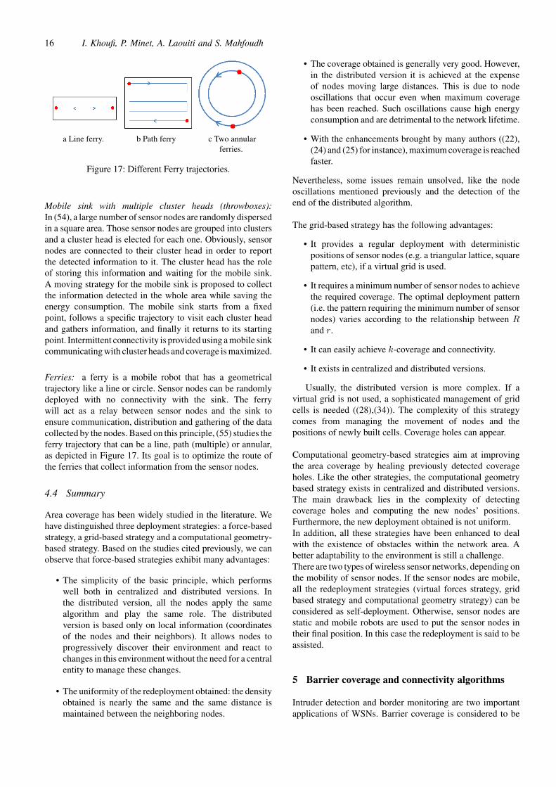
16 I. Khoufi, P. Minet, A. Laouiti and S. Mahfoudh
a Line ferry. b Path ferry c Two annularferries.
Figure 17: Different Ferry trajectories.
Mobile sink with multiple cluster heads (throwboxes):In (54), a large number of sensor nodes are randomly dispersedin a square area. Those sensor nodes are grouped into clustersand a cluster head is elected for each one. Obviously, sensornodes are connected to their cluster head in order to reportthe detected information to it. The cluster head has the roleof storing this information and waiting for the mobile sink.A moving strategy for the mobile sink is proposed to collectthe information detected in the whole area while saving theenergy consumption. The mobile sink starts from a fixedpoint, follows a specific trajectory to visit each cluster headand gathers information, and finally it returns to its startingpoint. Intermittent connectivity is provided using a mobile sinkcommunicating with cluster heads and coverage is maximized.
Ferries: a ferry is a mobile robot that has a geometricaltrajectory like a line or circle. Sensor nodes can be randomlydeployed with no connectivity with the sink. The ferrywill act as a relay between sensor nodes and the sink toensure communication, distribution and gathering of the datacollected by the nodes. Based on this principle, (55) studies theferry trajectory that can be a line, path (multiple) or annular,as depicted in Figure 17. Its goal is to optimize the route ofthe ferries that collect information from the sensor nodes.
4.4 Summary
Area coverage has been widely studied in the literature. Wehave distinguished three deployment strategies: a force-basedstrategy, a grid-based strategy and a computational geometry-based strategy. Based on the studies cited previously, we canobserve that force-based strategies exhibit many advantages:
• The simplicity of the basic principle, which performswell both in centralized and distributed versions. Inthe distributed version, all the nodes apply the samealgorithm and play the same role. The distributedversion is based only on local information (coordinatesof the nodes and their neighbors). It allows nodes toprogressively discover their environment and react tochanges in this environment without the need for a centralentity to manage these changes.
• The uniformity of the redeployment obtained: the densityobtained is nearly the same and the same distance ismaintained between the neighboring nodes.
• The coverage obtained is generally very good. However,in the distributed version it is achieved at the expenseof nodes moving large distances. This is due to nodeoscillations that occur even when maximum coveragehas been reached. Such oscillations cause high energyconsumption and are detrimental to the network lifetime.
• With the enhancements brought by many authors ((22),(24) and (25) for instance), maximum coverage is reachedfaster.
Nevertheless, some issues remain unsolved, like the nodeoscillations mentioned previously and the detection of theend of the distributed algorithm.
The grid-based strategy has the following advantages:
• It provides a regular deployment with deterministicpositions of sensor nodes (e.g. a triangular lattice, squarepattern, etc), if a virtual grid is used.
• It requires a minimum number of sensor nodes to achievethe required coverage. The optimal deployment pattern(i.e. the pattern requiring the minimum number of sensornodes) varies according to the relationship between Rand r.
• It can easily achieve k-coverage and connectivity.
• It exists in centralized and distributed versions.
Usually, the distributed version is more complex. If avirtual grid is not used, a sophisticated management of gridcells is needed ((28),(34)). The complexity of this strategycomes from managing the movement of nodes and thepositions of newly built cells. Coverage holes can appear.
Computational geometry-based strategies aim at improvingthe area coverage by healing previously detected coverageholes. Like the other strategies, the computational geometrybased strategy exists in centralized and distributed versions.The main drawback lies in the complexity of detectingcoverage holes and computing the new nodes’ positions.Furthermore, the new deployment obtained is not uniform.In addition, all these strategies have been enhanced to dealwith the existence of obstacles within the network area. Abetter adaptability to the environment is still a challenge.There are two types of wireless sensor networks, depending onthe mobility of sensor nodes. If the sensor nodes are mobile,all the redeployment strategies (virtual forces strategy, gridbased strategy and computational geometry strategy) can beconsidered as self-deployment. Otherwise, sensor nodes arestatic and mobile robots are used to put the sensor nodes intheir final position. In this case the redeployment is said to beassisted.
5 Barrier coverage and connectivity algorithms
Intruder detection and border monitoring are two importantapplications of WSNs. Barrier coverage is considered to be

Coverage and Connectivity Issues and Challenges in WSN 17
an appropriate model for such applications. A deployment ofsensor nodes along a barrier is necessary to detect an intrudercrossing, for example, an international border. Dependingon the application requirements and the number of sensornodes provided, this deployment can ensure either full barriercoverage or partial barrier coverage.
5.1 Full barrier coverage
Full barrier coverage can be either simple or multiple. It issimple, if there is just one barrier that is fully covered bysensor nodes. The barrier coverage is multiple if there are ksuccessive barriers of sensor nodes.The authors in (48) are the first to address the problem ofproviding the minimum number of deployed sensor nodesto ensure simple or multiple barrier coverage. They definea simple barrier coverage by a belt of successive sensornodes such that their sensing areas overlap. A multiple barriercoverage is defined by the fact that every two successivebarriers have two overlapping sensor nodes, as depicted inFigure 18b. Based on a theoretical study, the authors provethat the optimal number of sensor nodes deployed along abarrier is l
2r , where l is the length of the barrier and r thesensing range. Then, every two successive sensor nodes areat a distance of 2r in order to optimize the overlapping (seeFigure 18a). To ensure full barrier coverage, two types ofdeployment algorithms can be used, depending on whethersensor nodes are static or mobile.
a Optimal 1-barriercoverage.
b The above zone is2-barrier covered.
Figure 18: Barrier coverage.
5.1.1 Static sensor nodes
When sensor nodes are static, they are generally deployeduniformly over the whole area based on a Poisson PointProcess model. Using this kind of deployment, barriercoverage can be provided by selecting a chain of overlappingsensor nodes. However, when static sensor nodes are droppedby an aircraft, they will deviate from their expected locationdue to mechanical inaccuracy or environmental factors suchas wind, terrain characteristics, etc. To cope with this problem,(50) proposes a concentrated deployment of sensor nodesalong the deployment line with some random offsets, usingfor example aircraft (see Figure 19). This distribution is calledLNRO, Line based normal random offset distribution, and interms of barrier coverage, it outperforms the Poisson modelwhen the random offset in LNRO is relatively small comparedto r.
5.1.2 Mobile sensor nodes
A deployment strategy to ensure (simple or multiple) barriercoverage using mobile sensor nodes is proposed in (49). Thisstrategy consists in dividing the area into virtual lines (i.e.barriers) where the number of virtual lines matches the desiredrobustness of barrier coverage. In each line, sensor nodesshould occupy grid points at a distance of 2r. Starting from arandom deployment in a rectangular area, mobile sensor nodesshould execute two phases to reach their final positions. In thefirst phase, each sensor node moves vertically to reach a line.Then, in the second phase, it moves horizontally along the lineto a predetermined grid point position. When each grid pointis occupied by a sensor node, full barrier coverage is provided.
Figure 19: LNRO barrier deployment.
(51) focuses on finding and healing barrier holes usingmobile sensor nodes. This work is an extension of (50).After the deployment, sensor nodes may fail due to manyfactors, such as battery depletion, environmental conditionsor malfunctioning. Then, a redeployment is needed to healcoverage holes. The proposed algorithm proceeds in twophases. In the first phase, it scans the network from thebeginning to the end of the barrier to check coverage holes. Thesecond phase consists in computing which sensor nodes shouldmove to which position such that the total distance traveledby the nodes is minimized. This algorithm takes advantage ofthe LNRO distribution as all sensor nodes are concentratedalong a line, as depicted in Figure 19, allowing quick and easyreplacement of failed nodes.
a Big object: 1-barriercoverage.
b Small object:2-barrier coverage.
Figure 20: Dynamic object.
The monitored object may be dynamic, (i.e. changing itsshape). As a consequence, sensor nodes have to move to adaptthe belts they form around the object to be monitored. In(52) the problem of mobile barrier for dynamic coverage isformulated as: for a given number n of sensor nodes, howdo sensor nodes move with the objective to minimize the

18 I. Khoufi, P. Minet, A. Laouiti and S. Mahfoudh
total distance traveled under the constraint that the number ofbarriers is maximized at any time. Sensor nodes are placedaround the dynamic object, neighboring sensors are at adistance less than or equal to 2r forming a belt around thedynamic object without any coverage holes. The authorsassume that R ≥ 2r, in order to ensure full connectivity. Adynamic belt region provides k-mobile barrier coverage if andonly if there are k vertex disjoint belts in its coverage graph.The maximum number of barriers k changes in response tochanges of the dynamic object, k becomes smaller when thedynamic object becomes larger, as illustrated in Figure 20.
5.2 Partial barrier coverage
In the barrier coverage problem, the optimal number of nodes(denoted m points) required to fully cover the barrier, can bedetermined based on the sensors’ sensing range and the barrierlength. However, if the number of available nodes is less thanoptimal, the barrier coverage problem will be formulated ashow to movenmobile sensor nodes to monitorn points amongthe m points so as to maximize the average intruder detectionwhile minimizing the average sensor movement distance. Tosolve this problem, two algorithms PMS and CSP are proposedin (53). PMS, periodic monitoring scheduling, lets sensornodes monitor each point of the barrier periodically, regardlessof any arrival by an intruder and without any coordinationbetween sensors. Each sensor moves to the point j and staysthere for T time slots. Then, it moves to pointmod(j + n,m)and stays there, also for T time slots. This is repeated untilall the sensors run out of energy. CSP, Coordinated Sensorpatrolling, is a centralized algorithm that uses the temporalcorrelation of intruder arrival times. CSP runs in two steps.Firstly, it selects the point with the highest priority of intruderarrival to be monitored at the current time. Then, it determineshow to move sensors to the selected point while minimizingthe total distance traveled, using the information collected inthe past time slot. It has been shown that the CSP algorithmoutperforms PMS.
5.3 Summary
Generally, the barrier coverage problem refers to criticalapplications such as intruder detection which require specialattention. The high degree of robustness (multiple barriercoverage) is generally chosen for critical applications to provethe efficiency and reliability of the monitoring task.Furthermore, the zone monitored, such as a battlefield orcountry borders very often includes obstacles and is not alwaysflat in these applications. Many environment constraintsmay occur, such as in a battlefield or international borders.Obstacles can also occur in the monitoring barrier. Thesolutions proposed in the literature do not take into accountthese constraints which have a negative impact on thedeployment algorithm.The issue of connectivity is very important in criticalapplications since it allows information to be reported tothe sink. All the papers cited in this section, assume thatconnectivity between neighboring nodes and with the sink isensured:R ≥ 2r. However, in real deployments, this condition
is not always met. In such a case, strategies to ensureconnectivity should be provided.Sensor nodes may be dropped randomly, trying to follow abarrier line (e.g. (50)). In this case, coverage can be improvedby a centralized algorithm, as in (51) in charge of detecting andhealing holes in barrier coverage. However, when coverageholes are present, the central entity may fail to collect all sensornodes’ positions since these holes may produce disconnectedcomponents.
6 Point coverage and connectivity algorithms
The last type of coverage is given by the coverage of Points ofInterest (PoI). Examples of applications include the detectionof some static or moving target, using the smallest number ofsensors. We distinguish between static PoIs and dynamic PoIs.
6.1 Static PoI
In (47), the authors are interested in the deployment ofmobile sensors to cover predefined PoIs, while preservingconnectivity with the sink. The sink has the task ofdisseminating information about the PoI locations to thesensors as well as collecting the information reported fromthe sensors about the events happening at the PoI. The basicidea of this deployment algorithm for PoI coverage is asfollows: initially all the sensors are within radio range of thesink. All the sensors run the same algorithm but the motiondecision is taken individually by each sensor node. The sensorsmove toward one predefined point that could be the PoI orthe barycenter of the PoIs. Then they form straight linesbetween the PoI and the sink. The distance the sensors moveis bounded in order to maintain connectivity. Finally a sensorstops moving, when it covers the PoI (i.e. the PoI is in thesensing range of the sensor). The strategy of this deploymentalgorithm minimizes the number of sensors used to maintainconnectivity by using the RNG graph (Relative NeighborhoodGraph).
If multiple PoIs exist in the area considered, twoapproaches can be adopted:
• Random PoI deployment: the sensor chooses one of thePoI at random;
• Barycenter PoI deployment: Every sensor calculates thebarycenter of all the PoIs and the sink to cover it. Thenany sensor chooses a PoI at random and covers it.
In (44), a distributed deployment scheme is proposedwhere mobile sensors nodes move following concentriccircular paths (ferries with annular trajectories) that coverstatic PoIs (See Figure 21). The goal of this work is to ensurePoI coverage and that events are reported to the sink. This sinkis located at the barycenter. Two neighboring circular pathsare at a distance of R. The authors assume that R ≥ 2r andmobile sensors have no global knowledge of the PoIs in thearea considered. This work combines three aspects which are:PoI discovery, PoI coverage and connectivity with the sink.To achieve these three aspects, a mobile sensor should move

Coverage and Connectivity Issues and Challenges in WSN 19
constantly to execute the PoI discovery task. Then, it shouldadjust its movement velocity with sensors in the neighboringcircular paths to satisfy the constraints regarding coverage andconnectivity with the sink in order to report the informationabout the PoIs.
Figure 21: PoI coverage using annular ferries.
Temporary coverage of Multiple PoIs is studied in (45)and is called the sweep coverage problem as sensor nodessweep between PoIs and cover them periodically. A distributedalgorithm DSWEEP is proposed to address this problem.A sensor node covers a PoI for a determined duration andthen moves to a new one. When a sensor node is moving, itencounters other sensor nodes and exchanges information thatserves to decide which PoI should be monitored next. Thisdeployment algorithm needs a small number of sensor nodesto cover a large number of PoIs. DSWEEP provides temporarycoverage and partial network connectivity.In some applications, the PoI, as well as the area surroundingit need to be covered. In (46) a localized self deploymentalgorithm is proposed to meet this goal. This algorithm is basedon a virtual triangular lattice grid of edge
√3r to maintain
connectivity since it is assumed that R ≥√3r. Sensor nodes
are autonomous and know the position of the PoI. They movethrough the triangular vertexes and organize themselves byrespecting rules that avoid collisions between sensors, to reachthe vertices around the PoI. Based on this principle no coverageholes will occur if all the vertexes around the PoI are occupiedby sensor nodes.
a Initial deployment. b Final deployment.
Figure 22: PoI coverage using Grid.
6.2 Mobile PoIs
In the case of mobile PoIs, the authors of (47) propose threestrategies to reach the mobile PoI:
• In the first strategy, sensor nodes move back to thesink before deploying toward the new location of thePoI. This strategy provides a high coverage quality butincreases the deployment duration and the amount ofenergy consumed.
• In the second strategy, sensors try to move directly towardthe new location of the PoI without going back to thesink. This strategy reduces the time needed to cover thenew PoI but also reduces the coverage quality as it needsa greater number of sensors to maintain connectivity.
• In the third strategy, a sensor moves toward the straightline between the sink and the new location of PoI, thenit moves toward the PoI. This strategy provides a highercoverage quality and reduces the time needed to coverthe PoI.
6.3 Summary
Any PoI needs only one sensor to be covered. If permanentconnectivity is required, a sufficient number of sensor nodesare deployed to ensure connectivity with the sink. However,if intermittent connectivity is sufficient, one sensor node willcover a PoI, and a mobile node (that can be the sink or acollector Robot) will operate like a data mule. This can be asolution to deploy a minimum number of sensor nodes andsave energy.When the PoI is static, a static sensor node can be used to coverit. If the PoI is mobile, however, autonomous sensor nodes aredeployed to track the PoI and avoid the use of a robot thatwould pick up and deploy sensor nodes each time the positionof the PoI changes.Notice that PoI coverage needs just one sensor to be covered,whereas a zone of interest requires at least one sensor to becovered as the zone may be larger than the sensors’ sensingrange. When many sensor nodes are deployed to cover azone (area) of interest, they are usually deployed with variousdensities: high density in the center of the zone of interest andthen the density decreases with the distance to the center ofthe zone.
7 Node activity scheduling with regard to coverage
Assuming an initial deployment of static sensor nodes meetingthe application requirements (e.g. full or partial coverage),the node activity scheduling problem consists in determininga connected set of active nodes to ensure the applicationrequirement. Only nodes in this set are active, the other nodesare sleeping to save energy. Hence, the network lifetime ismaximized. The problem here is not to deploy the sensornodes but only to select which sensor nodes will be active tomaximize coverage and connectivity. Figure 23 depicts anexample where blue sensor nodes are sleeping, while coverageand connectivity are ensured by white sensor nodes in red.

20 I. Khoufi, P. Minet, A. Laouiti and S. Mahfoudh
Figure 23: Node Activity Scheduling.
We distinguish two categories of node activity schedulingwith regard to coverage:
7.1 Node activity scheduling based on messageexchanges between neighbors
Sensor nodes rely on message exchanges to decide whichsensor nodes should be in an active state while others aresleeping, with the goal of ensuring full coverage and savingenergy. This mechanism can either be centralized, where acentral entity collects all the nodes’ positions and assignsa state (active or sleep) to each node, or distributed, whereneighboring sensor nodes exchange messages to decide whichof them will be active while others are sleeping.An example of a centralized algorithm is given in (17). Thiswork is based on the construction of a connected subgraph ofsensor nodes based on local information. It focuses on findingthe smallest subset of sensor nodes that ensures full coverageof the monitored area while maintaining connectivity with thesink.Another centralized algorithm is proposed in (59) to build acamera barrier from an initial arbitrary deployment of camerasensors. The aim is to guarantee that each point of the barrieris fully covered visually. The method consists in building agraph of nodes where each of them covers a small subregion,and every two adjacent nodes are connected. The idea is toselect a path from one boundary to another such that the nodesof the path are full-view covered. Only nodes belonging to thatpath are active.Node activity scheduling based on message exchanges is alsoadopted to ensure partial coverage. In (57), a centralizedalgorithm is proposed to ensure partial coverage. It aims toselect the smallest number of nodes to monitor p-percent ofthe area. The authors also propose a distributed algorithm thatdetermines a set of nodes to cover p-percent of the consideredarea. The main idea of these two algorithms is to divide thewhole area into sub-regions and select specific nodes, whilerespecting some criteria (for example, a starter node selectsits furthest neighbor) in order to cover p-percent of each sub-region.CCP, Coverage Configuration Protocol (12) is a distributedalgorithm based on message exchanges to provide the degreeof coverage required by applications when R ≥ 2r. In CCP,according to information about its sensing neighbors, a sensornode can be in a sleep state to save energy, a listen state tocollect neighboring messages and decide its new state, or anactive state to sense the environment. Without assuming thatR ≥ 2r, CCP cannot guarantee network connectivity. In (12),CCP is combined with SPAN (14) to achieve both coverage
and connectivity when R < 2r. SPAN is a connectivitymaintenance protocol. This protocol connects all active nodesvia a communication backbone, and connects inactive nodesto at least one active node. Then, when R < 2r, networkconnectivity is ensured.Several other distributed protocols are proposed in (18), toensure area coverage with a low communication overhead. Inthese protocols sensor nodes select a waiting time for eachround and receive neighboring messages which are used tocompute the area coverage. If the sensing area of a sensornode is not fully covered, the node should stay in an activestate during the current round and announce its state when itswaiting time expires.Sensing range and radio range may be different and they mayalso differ between sensor nodes. The authors in (19) adoptthis assumption and aim to minimize the number of activenodes in the region queried that is fully covered. Then, eachsensor node should determine whether it switches to an activestate to respond to the query request originating from the sink,based on information collected from its neighbors.
7.2 Node activity scheduling based on implicitcoordination
Implicit coordination algorithms are proposed to savethe energy of sensor nodes, assuming full coverage andconnectivity. Such algorithms are distributed and based on agrid. Each node knows from its position in the grid whetherit must be active or it can sleep. An example is given in (15)for a square pattern and a hexagonal pattern: each sensornode located in the vertex of the grid switches to the activestate, while other nodes are sleeping. Another example of asquare pattern is given in by VFCSO, Virtual Force-BasedCoverage Optimization Strategy (26). VFCSO is a dynamicdeployment algorithm that aims at ensuring full area coverageusing a minimum number of sensor nodes while saving energyconsumption. In this work, the considered area is divided intosquare cells with edges equal to r. Many sensor nodes may bein the same square cell. Starting from a random deployment,the virtual forces strategy is applied by sensor nodes belongingto the same square cell. Only one node in each cell will beactive, the others should switch to the sleep state: the activenode being the closest sensor node to the center of the cell withthe highest residual energy. Both full coverage and networkconnectivity are guaranteed in this work as R ≥
√5r.
8 Some considereations for practitioners
In this section we set out to help designers to selecta deployment algorithm that meets their applicationrequirements, and give some recommendations.The two main questions that the designer has to consider arethe following:
• What does the application need in term of coverage andconnectivity?
• Which assumptions and constraints are given?

Coverage and Connectivity Issues and Challenges in WSN 21
In the following we discuss various ways to answer thesequestions.IDefinition of the coverage and connectivity problem thatmust be solved:
• Coverage− If the goal is to monitor an area, then the problemconcerns area coverage, which may be full or partial.If it is to detect barrier crossing, the problem is barriercoverage, which, again, may be full or partial.If the goal is to track/monitor a target, the problem dealswith point of interest (PoI) coverage. The PoI may bestatic or mobile.− If coverage must be full and the degree of robustnessrequired by the application is high, multiple coverage isneeded, otherwise simple coverage is sufficient.− If long delays to detect an event are tolerated by theapplication, the coverage of any point can be temporary.Otherwise, it is permanent.
• Connectivity− If short delays to report detected events to the sinkare required by the application, permanent connectivitymust be ensured. Otherwise, intermittent connectivity issufficient.− If the application needs a high degree of robustness,multiple paths to the sink should be maintained.Otherwise, a simple path
• Type of deployment− depending on the application requirements, a uniformand regular deployment should be provided, based on apattern (see Section 3.3).
I Assumptions and constraintsIn most cases, the designer will be faced with multipleassumptions and constraints that must be taken into accountwhen selecting the appropriate deployment algorithm. Theseinclude:
• Environment− The dimensions and position of the area, barrier orPoI to cover should be provided in order to computethe minimum number of sensor nodes required. If thisnumber is large, the deployment algorithm must bescalable. The initial topology influences the deploymentalgorithm, specially when some sensor nodes aredisconnected, or when they are all grouped together at anentry point (see the discussion in Section 3.1).− The choice of the radio propagation model mustbe compliant with the environment (e.g. free space orconfined) which may suffer from perturbations caused byother wireless networks (e.g. WiFi) or electronic devices(e.g. microwaves), and may also contain obstacles.− In the presence of obstacles, detection and get aroundtechniques should be provided.
• Sensor nodes− Mobility: sensor nodes may be mobile andautonomous, and this condition is necessary for self-deployment. On the other hand, static nodes should be
assisted in their deployment by a mobile robot.− The sensing range r, the communication range R andthe associated models: for more details see Section 3.2.Furthermore, the relationship between r and R will beused to select the appropriate deployment algorithms inTable 3.− The number of sensor nodes must be sufficient to meetthe application requirements, otherwise the problem isimpossible to solve.− Energy: if sensor nodes are equipped with a battery,the deployment algorithm must be energy efficient.
• The sinkIt is in charge of collecting the data generated by thesensor nodes deployed. It can be static or mobile. If thesink is static, either it is connected to sensor nodes, ora mobile robot visits the disconnected sensor nodes tocollect their data and report them to the sink. If the sinkis mobile, it moves to collect data.
I Recommendations:
• Coverage problemDepending on the application needs, the problem is anarea, barrier or PoI (Point of interest) coverage problem.
• Relationship between the transmission range R and thesensing range rThe relationship between R and r influences the choiceof the solution. If for instance R ≥
√3r, it is sufficient
to solve the coverage problem to obtain connectivity asa consequence of coverage. If the transmission range Ris strictly less than the sensing range r, a distributeddeployment would require a smaller target distancebetween sensor nodes than that required by full coverageof the area. Hence, a higher number of sensor nodes isused, leading to a more expensive solution. If the designerhas a small budget, he/she will prefer a centralizedsolution with a mobile robot/agent to deploy the sensornodes to their final position, and to collect data fromthese nodes in the data gathering phase. Similarly, such asolution is also preferred when the application toleratesdelays (e.g. delay tolerant networks, ferries). In contrast,a permanent path must exist from any sensor node to thesink. Additional sensor nodes are required to ensure thispermanent connectivity.
• Centralized versus Distributed solutionDepending on the area/barrier size, a centralized/distributed solution will be preferable. Indeed, ifthe monitoring requires a high number of sensors,a distributed solution is chosen because of its betterscalability, provided that the energy constraints are takeninto account, as discussed below. A centralized solutionrequires that the central entity in charge of the deploymentcomputation has perfect knowledge of the positions of allthe sensor nodes. If the initial topology is disconnected,a mobile robot is needed to collect the initial positions ofall disconnected nodes to compute the final deployment.If all sensor nodes are static, the centralized solution is

22 I. Khoufi, P. Minet, A. Laouiti and S. Mahfoudh
the only possible one. A mobile robot is needed to deploythe sensor nodes to their final position.
• Energy constraintsWhen sensor nodes are equipped with a battery of limitedcapacity, energy efficient techniques should be used.Special care must be given to node activity schedulingthat allows nodes to sleep for energy saving purposes.Another advantage of node activity scheduling is tomake the deployment adaptive to varying coveragerequirements, ranging from full to partial. However, theenergy consumed by nodes movements is considerableand should be limited. For instance, nodes oscillationsoccurring in some distributed solutions should beavoided. If the designer wants to keep the energy of sensornodes for data gathering, a mobile robot/agent should beused to deploy the sensor nodes to their final position.
• Uniform and regular deploymentA uniform and regular deployment reduces the energyconsumed during the data gathering phase and minimizesthe data gathering delay. Moreover, it provides better timeand space consistency of the measures reported to thesink.
• ObstaclesAn area/barrier with obstacles needs mechanisms todetect obstacles and strategies to get around them, as wellas ensuring the required coverage.
9 Trends and open issues for deployment algorithms
Deployment is a fundamental issue in WSNs. Many challengeshave been studied and published in the literature. In this survey,we have discussed and classified some of them according totheir main characteristics with a special focus on coverage andconnectivity.Nevertheless, several issues are still unresolved or understudy to achieve an optimized deployment that can beadapted to different situations and emerging technologies. Webelieve that the sensors’ devices will become more powerfulwith enhanced capacities, like more sophisticated processing,greater sensing range, fully equipped with positioning systemand integrating more and more various sensing componentsas well as actuators. Some of them could even embed severalcommunication technologies (802.15.4, WiFi, 3G, 4G).In short, sensor devices are becoming faster, more intelligentand heterogeneous. However, their autonomy is still limitedby their embedded energy. Pushing back this boundary, energyharvesting and renewable energy are promising techniques toextend the lifetime of a battery and hence make them moreautonomous.Since sensor devices are becoming cheaper, they can bedeployed on a large scale to build more complex wirelessnetworks offering more functionalities. To provide scalability,distributed algorithms are more suitable than the centralizedones.These trends will increase with the emergence of the Internetof Things, where sensors and actuators embedded in physical
objects communicate through wired or wireless networks thattend to use common internet protocols (e.g. IP).The deployment algorithms presented in this survey deal onlywith 2D. With new applications in smart cities, sensors willbe deployed in 3D. For instance, sensors can be fixed on theground, as well as at different heights on buildings to form anetwork.The radio propagation models are different and newdeployment algorithms should be designed. With theintroduction of UAVs (Unmanned Aerial Vehicles) andMUAVs, (Micro UAVs), swarms of flying and communicatingUAVs and MUAVs will be used in monitoring applications.The main characteristics of such networks are the coordinatedmoves to deploy and redeploy in a 3D space to meet theapplication requirements. Similarly to 3D deployments in theair, exist 3D underwater deployments based on ultrasoundcommunication. Both 2D and 3D deployment algorithmshave to cope with positioning errors, which are common inpositioning systems like GPS. Few algorithms take this issueinto account.Security is an important issue in deployment algorithms, but isusually not addressed. An intruder could harm the deploymentprocess and corrupt the data gathering.We expect that wireless sensor network technologies will bemature very soon and will be widely deployed in a large varietyof industrial applications requiring multihop communicationsand needing tight constraints. In these applications, specificattention should be paid to robustness. The deploymentalgorithms should be able to tolerate some message lossesand some failed sensor nodes. Furthermore, the deploymentalgorithms should be able to adapt to the dynamic changes ofthe application requirements during the monitoring task.Deployment algorithms need to be smarter in adaptingthemselves to changes in the environment or the applicationrequirements that could be more frequent.
10 Conclusion
In this survey, we studied two major challenges inWSNs: coverage and connectivity, while bearing in mindthe importance of energy issue. We provided indicationsfor analyzing deployment algorithms and evaluating theirperformances. We distinguish two types of deploymentalgorithms depending on the mobility of sensor nodes:self deployment for mobile sensor nodes and assisteddeployment for static sensor nodes deployed by mobilerobots. Deployment algorithms are designed to meet theapplication requirements such as coverage, connectivity,latency and robustness. We established a classification ofdeployment algorithms based on these requirements. Weprovide several recapitulative tables to help the reader gain abetter understanding of the advantages and shortcomings ofthe problems and algorithms studied. In fact, the deploymentof sensor nodes and sinks can be considered as the firststep in the design of a data gathering application. As asecond step, node activity scheduling is used to optimizeenergy consumption by switching off redundant nodes tomaximize network lifetime, while ensuring the coverage and

Coverage and Connectivity Issues and Challenges in WSN 23
connectivity required by the application. It should be notedthat the deployment provided determines the consumption ofenergy and bandwidth during the data gathering. The readerwill find useful guidelines to select the deployment algorithms,that are best-suited to his/her needs. The deployment ofwireless sensor nodes to monitor a temporary worksite isa typical use case representative of industrial applicationswhere full coverage and full connectivity are required.In precision farming, for instance, partial coverage withintermittent connectivity are sufficient to meet the applicationrequirements. The reader is also given an overview ofcurrent trends and some interesting open issues. We stronglybelieve that the deployment algorithms will undergo extensivedevelopment with the rapid emergence of the Internet ofThings.
Acknowledgment
This work has been partially funded by the Cluster Connexionproject. For more details see http://www.cluster-connexion.fr/We would like to thank Richard James for his help to improvethe quality of this survey.
References
[1] Y. Miao (2005) ’Applications of sensor networks’, SeminarWireless Self-Organization Networks.
[2] R. Mulligan and H. M. Ammari (2010) ’Coverage inWireless Sensor Networks: A Survey’, Networks protocols andalgorithms, vol. 2, no. 2.
[3] A. Ghosh and S. K. Das (2008) ’Coverage and ConnectivityIssues in Wireless Sensor Networks: A survey’, Pervasive andMobile Computing, vol. 4, I. 3, p. 303-334.
[4] G. Fan and S. Jin (2010) ’Coverage Problem in Wireless SensorNetworks: A Survey’, Journal of networks, vol. 5, no 9.
[5] B. Wang (2011) ’Coverage Problem in Sensor Networks: ASurvey’, ACM Computing Surveys, vol. 43 no.4, article 32.
[6] C. Zhu, C. Zheng, L. Shu and G. Han (2012) ’A survey oncoverage and connectivity issues in wireless sensor networks’,Journal of Network and Computer Applications, p. 619-632.
[7] S. Mahfoudh, P. Minet and A. Laouiti (2012) ’Overview ofDeployment and Redeployment Algorithms for Mobile WirelessSensor Networks’, Emerging Topic on Sensor Networks.
[8] M. C. Akewar and N. V. Thkur (2012) "Study of Wireless MobileSensor Network Deployment" Internatioal Journal of Computerand Wireless Communication, vol. 2, no 4.
[9] R. Soua, P. Minet, E. Livolant (2012) ’MODESA: an OptimizedMultichannel Slot Assignment for Raw Data Convergecast inWireless Sensor Networks’, IPCCC 2012, the 31st IEEEInternational Performance Computing and CommunicationsConference, Austin, Texas.
[10] H. Wang and W. Chung (2012) ’The generalized k-coverageunder probabilistic sensing model in sensor network’ WCNC.
[11] H. Zhang and J. C. Hou (2005) ’Maintaining Sensing Coverageand Connectivity in Large Sensor Networks’ Ad Hoc and SensorWireless Networks, vol. 1, no. 1-2.
[12] X. Wang, Y. Zhang, C. Lu, R. Pless and C. Gill (2003) ’IntegredCoverage and Connectivity Configuration in Wireless SensorNetworks’, SenSys, Embedded networked sensor systems, p. 28-39.
[13] X. Bai, S. Kumar, D. Xuan, Z. Yun and T.H. Lai (2006)’Deploying Wireless Sensors to Achieve Both Coverage andConnectivity’, MobiHoc, Mobile ad hoc networking andcomputing, p. 131-142.
[14] B. Chen, K. Jamieson, H. Balakrishnan and R. Morris(2001) ’Span: An Energy Efficient Coordination Algorithm forTopology Maintenance in Ad Hoc Wireless Networks’, ACMWireless Networks Journal.
[15] R. Lyengar, K. Kar and S. Banerjee (2005) ’Low-coordinationTopologies for Redundancy In Sensor Networks’, Mobihoc.
[16] K. Kar and S. Banerjee (2003) ’Node Placement forConnected Coverage in Sensor Networks’, WiOpt Modeling andOptimization in Mobile, Ad Hoc and Wireless Networks.
[17] J. Carle and D. Simplot Ryl (2004) ’Energy-Efficient AreaMonitoring for Sensor Networks’, IEEE Computer Society.
[18] A. Gallais, J. Carle, D. Simplot Ryl and I. Stojmenovic (2008)’Localized Sensor Area Coverage with Low CommunicationOverhead’, IEEE Transaction on mobile computing, vol. 7, no.5.
[19] J. P. Sheu, S. C. Tu and C. H. Yu (2007) ’A DistributedQuery Protocol in Wireless Sensor Networks’, Wireless PersonalCommunication, p. 449-464.
[20] Y. C. Wang, C. C. Hu and Y. C. Tseng (2005) ’EfficientDeployment Algorithms for Ensuring Coverage and connectivityof Wireless Sensor Networks’, WICON.
[21] Y. Zou and K. Chakrabarty (2003) ’Sensor Deployment andTarget Localization Based on Virtual Forces’ IEEE INFOCOM.
[22] K. Mougou, S. Mahfoudh, P. Minet and A. Laouiti (2012)’Redeployment of Randomly Deployed Wireless Mobile SensorNodes’ IEEE VTC, Quebec, Canada.
[23] S. Mahfoudh, I. Khoufi P. Minet and A. Laouiti (2013)’Relocation of Mobile Wireless Sensors in the Presence ofObstacles’, ICT, CasaBlanca, Marroco.
[24] J. Li, B. Zhang, L. Cui and S. Chai, (2012) ’An ExtendedVirtual Force-Based Approach to Distributed Self-Deployment inMobile Sensor Networks’, International Journal of DistributedSensor Networks.
[25] J. Chen, S. Li, and Y. Sun (2007) ’Novel Deployment Schemesfor Mobile Sensor Networks’ Sensors, vol. 7, no. 11, pp. 2907-2919.
[26] Q. Xu and Q. Wang (2012) ’Coverage OptimizationDeployment Based on virtual Force Directed in Wireless SensorNetworks’, IPCSIT, vol. 47, Singapore.
[27] G. Tan, S. A. Jarvis, A. M. Kermarrec (2009) ’Connectivity-Guaranteed and Obstacle-Adaptive Deployment Schemes forMobile Sensor Networks’, IEEE Transactions on MobileComputing.
[28] N. Bartolini, T. Calamoneri, E. G. Fusco, A. Massini and S.Silvestri (2010) ’Autonomous deployment of mobile sensors fora complete coverage’, Journal Wireless Networks, vol. 16, I. 3,p. 607-625.
[29] Y. H. Kim, C. M. Kim, D. S. Yang, Y. J. Ohand Y. H. Han(2012) ’Regular Sensor Deployment Patterns for p-Coverage andq-Connectivity in Wireless Sensor Networks’, ICOIN.
[30] Z. Yun, X. Bai, D. Xuan, T. H. Lai and W. Jia (2010) ’OptimalDeployment Patterns for Full Coverage and k-Connectivity (k ≤6)Wireless Sensor Networks’, IEEE Tansactions on Networking,vol. 18, no. 3.

24 I. Khoufi, P. Minet, A. Laouiti and S. Mahfoudh
[31] N. A. Ab. Aziz, K. Ab. Aziz, and W. Z. W. Ismail (2009)’Coverage Strategies for Wireless Sensor Networks’, WorldAcademy of Science Engineering and Technology.
[32] S. Han, Y. Zhang and G. Xu (2010) ’Hexagonal grid-based sensor deployment algorithm’, Control and DecisionConference, Chinese.
[33] P. Park, S. G. Min and Y. H. Han (2010) ’A Grid-based Self-deployment Schemes in Mobile Sensor Networks’.
[34] A. Mateska and L. Gavrilovska (2011) ’WSN Coverage andConnectivity Improvement Utilizing Sensor Mobility’, EuropeanWireless, Vienna, Austria.
[35] L. Xu, A. Nayak and I. Stojmenovic (2010) ’Back Trackingbased Sensor Deployment by a Robot Team’, Sensor Mesh andAd Hoc Communications and Networks, USA.
[36] K. Chan-Myung, Y. Dong-Sun, O. Young-jun and H. Youn-Hee (2012) ’Regular Sensor Deployment Patterns for p-coverageand q-connectivity in Wireless Sensor Network’,InformationNetworking ICOIN, 2012.
[37] Y. C. Wang and Y. C. Tseng (2007) ’Distributed DeploymentSchemes for Mobile Wireless Sensor Networks to Ensure Multi-level Coverage’ IEEE Transactions On Parallel And DistributedSystems.
[38] A. Raha, S. Maity, M. K. Naskar, O. Alfandi and D. Hogrefe(2012) ’An Optimal Sensor Deployment Scheme to Ensure MultiLevel Coverage and Connectivity in Wireless Sensor Networks’,Wireless Communications and Mobile Computing ConferenceIWCMC, Limassol.
[39] J. Beaudaux, A. Gallais and T. Razafindralambo (2010)’Multiple Coverage with Controlled Connectivity in WirelessSensor Networks’, ACM workshop on Performance evaluationof wireless ad hoc sensor and ubiquitous networks.
[40] G. Wang, G. Cao and T. F. La Porta (2006) ’Movement AssistedSensor Deployment’, IEEE Transactions on Mobile Computing,vol 5, no 6.
[41] S. Babaie and S. S. Pirahesh (2012) (Hole DetectionFore Increasing Coverage in Wireless Sensor Network UsingTriangular Structure’, International Journal of Computer ScienceIssues IJCSI, vol. 9, I. 1, no 2.
[42] M.E. Keskin, I. K. Altmel, N. Aras, C. Ersoy (2013)’Optimal Deployment, Scheduling and Routing for Maximizingthe Lifetime of a Wireless Sensor Networks With MultipleMobile Sinks’, Technical Report FBE-IE-02/2013-02, Instituteof Graduate Science and Engineering, Bogazici University,Istanbul.
[43] H. Tan, Y. Wang, X. Hao, Q. S. Hua and F. C.M. Lau (2010)’Arbitrary obstacles constrained full coverage in wireless sensornetworks’ In Wireless Algorithms Systems and Applications,Springer Berlin Heidelberg.
[44] M. Erdelj, E. Natalizio and T. Razafindralambo (2012) ’MultiplePoint of Interest Discovery and Coverage with Mobile WirelessSensors’ Computing Networking and Communications ICNC.
[45] W. Cheng, M. Li, K. Liu, Y. Liu, X. Li and X. Liao (2011)’Sweep Coverage with Mobile Sensors’, Mobile ComputingIEEE transactions, vol. 10, I. 11, November 2011.
[46] X. Li, H. Frey, N. Santoro and I. Stojmenovic (2011)’Strictly Localized Sensor Self-Deployment for Optimal FocusedCoverage’, IEEE Transactions on Mobile Computing, Vol. 10,No. 11.
[47] M. Erdelj, T. Razafindralambo and D. Simplot Ryl (2013)’Covering Points of Interest with Mobile Sensors’, IEEETransaction on Parallel and Distributed Systems, p. 32-43.
[48] S. Kumar, T. H. Lai and A. Arora (2005) ’Barrier Coverage withWireless Sensor’, MobiCom, Germany.
[49] A. Saipulla, B. Liu, G. Xing and J. Wang (2010) ’BarrierCoverage with sensor of limited mobility’, MobiHoc, USA.
[50] A. Saipulla, C. Westphal, B. Liu, J. Wang (2009)’Barrier Coverage of Line-Based Deployment Wireless SensorNetworks’, INFOCOM, Rio de Janeiro.
[51] A. Saipulla, C. Westphal, B. Liu and J. Wang (2013) ’Barriercoverage with line-based deployed mobile sensors’ Journal AdHoc Network.
[52] L. Kong, Y. Zhu, M. Y. Wu and W. Shu (2012) ’Mobile BarrierCoverage for Dynamic Objects in Wireless Sensor Networks’,Mobile Adhoc and Sensor Systems MASS, Las Vegas, NV, USA.
[53] H. Shibo, C. Jiming, L. Xu, S. Xuemin and S. Youxian (2012)’Cost-Effective barrier coverage by mobile Sensor Network’,IEEE INFOCOM.
[54] E. M. Saad, M. H. Awadalla and R. R. Darwish (2008) ’A DataGathering Algorithm for a Mobile Sink in Large-Scale SensorNetworks’, Wireless and Mobile Communications, ICWMC,Athens.
[55] V. Kavitha and E. Altman (2010) ’Analysis and Design ofMessage Ferry Routes in Sensor Networks using Polling Models’Modeling and Optimization in Mobile, Ad Hoc and WirelessNetworks (WiOpt), Avignon.
[56] Y. Liu and W. Liang (2005) ’Approximate coverage inwireless sensor networks’, IEEE Conference on Local ComputerNetworks, Sydney.
[57] Y. Wu, C. Ai, S. Gao, and Y. Li (2008) ’p-Percent Coverage inWireless Sensor Networks’, WASA, Berlin.
[58] M. Hefeeda and M. Bagheri (2007) ’Wireless Sensor Networksfor Early Detection of Forest Fires’, Mobile Adhoc and SensorSystems, Pisa.
[59] Y. Wang and G. Cao (2011) ’Barrier Coverage in Camera SensorNetworks’, MobiHoc, Paris.